MEASURING TOTAL FACTOR PRODUCTIVITY AND … · 3 MEASURING TOTAL FACTOR PRODUCTIVITY AND VARIABLE FACTOR UTILISATION: SECTOR APPROACH, THE CASE OF LATVIA INTRODUCTION With the increasing

1

MEASURING TOTAL FACTOR PRODUCTIVITY AND VARIABLE FACTOR UTILISATION: SECTOR APPROACH, THE CASE OF LATVIA

CONTENTS

Abstract 2 Introduction 3 1. Factor Utilisation and Total Factor Productivity Growth: Theoretical Framework 6 2. Factor Inputs 9

2.1 Data 9 2.2 Quality Adjustment of Labour Inputs and Capital Services 10

3. TFP Estimation Results 13 Conclusions 22 Appendices 24 Bibliography 38

ABBREVIATIONS BEA – Bureau of Economic Analysis (US) CSB – Central Statistical Bureau of Latvia EU – European Union GDP – gross domestic product OECD – Organisation for Economic Co-operation and Development TFP – total factor productivity US – United States of America

2


ABSTRACT

This research constructs estimates of total factor productivity (TFP) growth for six sectors of the Latvian economy for the period 2000–2008, using a sectoral quarterly data set. Estimates are obtained by controlling for qualitative changes in production factors and assuming a mechanism for capturing changes in the utilisation of labour and capital. The paper delivers two main results. First, the use of indicators for labour and capital utilisation intensity allows for minimisation of fluctuations in the TFP measure and makes it less output growth dependent compared with the Solow residual approach. Second, the comparison of both methods shows that the estimate of the TFP growth obtained by the Solow residual approach might be undervalued for manufacturing, electricity, gas and water supply, wholesale and retail trade as well as hotels and restaurants, while overvalued for the growth in the transport, storage and communication sector of the Latvian economy.

Keywords: Total Factor Productivity, Solow residual, factor utilisation

JEL Classification numbers: C22, D24

The views expressed in the publication are those of the authors, employees of the Bank of Latvia Monetary Policy Department. The authors assume responsibility for any errors or omissions.

3


INTRODUCTION

With the increasing recognition that productivity growth is a key to sustained economic expansion, measuring productivity is becoming more important to economists and policy makers, hence a number of studies have appeared in the field of measuring productivity growth.

The history of growth theory shows that researcher usually rely on two big groups, i.e. exogenous (neoclassical) and endogenous, growth models. Models in the first group represented in the studies of F. P. Ramsey (21), R. M. Solow (23), T. W. Swan (25), D. Cass (5), and T. C. Koopmans (13) assume perfect competition, constant returns to scale, and diminishing returns to inputs. The long-term growth of productivity is exogenous and is determined outside the model. The standard measure of exogenous total factor productivity (TFP) growth, the Solow residual, is calculated as a part of output growth that cannot be accounted for by primary factors of production.

Researchers' interest in estimating long-term growth rate within a model gave an impulse to the development of endogenous growth models, first represented in the studies of P. M. Romer (22) and R. E. Lucas (14) who made use of assumptions about imperfect competition, possible increasing returns to scale, and constant returns to inputs. In recent analyses of endogenous growth models, researchers pay attention to the role of R&D activities, externalities, and human capital in determining the growth rate of technology.(1)

In earlier studies by A. Meļihovs and G. Dāvidsons (15), K. Beņkovskis and D. Stikuts (4), and D. Stikuts (24), the first of the above mentioned approaches used in determining production function parameters and estimating productivity growth for Latvia, i.e. an exogenous growth model, is applied. For the estimation of output gap, D. Stikuts (24) used an equation in which the value of capital cost share in production function is 0.225, and productivity growth is calculated as a Solow residual. K. Beņkovskis and D. Stikuts (4) obtained the value of capital cost share (0.319) and annual productivity growth rate (4.6%) through calibrating them around the sample mean value. In their work, A. Melihovs and G. Davidsons (15) constructed a standard Cobb–Douglas production function using a productivity growth time series which was calculated by applying the Kalman filter technique under the assumption that the value of capital cost share was 0.303. The respective estimated productivity growth rate proved to be rather unstable: the TFP growth was close to zero during the period of the 1998 Russian financial crisis and rising after Latvia's accession to the EU.

The estimations of TFP growth for Latvia referred to above do not reflect such variations in output that cannot be explained solely by input changes. Therefore, in order to account for changes in productivity that occur due to changes in efficiency, technological properties or cyclical effects, the authors made an attempt to improve the productivity measure for Latvia by applying a method proposed by S. Basu and M. S. Kimball (3) and its modifications used in the studies by S. Basu et al. (2) and C. Groth et al. (7; 8). This method allows the authors of this study to assess the TFP growth in the economy using several additional assumptions: first, the assumption about additional costs of input factors (costs of installing new equipment), and,

4


second, the assumption about non-constant factor utilisation intensity (intensity of input factor utilisation may differ in different business cycle periods, e.g. output decreases in response to demand shocks). The TFP growth is estimated at the sector level thus enabling the application of the "bottom-up approach" in assessing the productivity growth rate for economy overall. An important feature of the method is advanced measurement of factor inputs representing qualitative and structural changes of production factors.

As a result of the supplements above, three main improvements have been made in the calculation of TFP growth for Latvia: 1) data measurement has been advanced, 2) a mechanism for including factor utilisation intensity and cost adjustments in the model has been improved, and 3) the "bottom-up approach" has been used when calculating productivity growth for the main sectors of the Latvian economy.

TFP growth is estimated at the sector level using a quarterly data set for three services sectors and three goods-producing industries covering the period from 1999 to 2008. Represented are manufacturing (D), electricity, gas and water supply (E), construction (F), wholesale and retail trade, repair of motor vehicles, motorcycles and personal and household goods (G)1, hotels and restaurants (H), and transport, storage and communication (I)2. In 2008, the above sectors accounted for 67.5% of the total output. The "bottom-up approach" allows for analysing whether input factors and their utilisation intensity explain the performance differences across sectors.

In order to generate accurate measures of TFP, capital and labour time series are adjusted for qualitative and structural changes in the time series. The total labour force is obtained by weighting the number of unemployed in three levels of education by the respective average annual wages; the total capital stock is calculated by weighting book values of four asset groups by the respective rental price of capital.

The TFP growth for each sector is calculated by the two-stage least squares method (2SLS) with demand side instruments. The estimated regression equations have four main parts: 1) a constant, representing the trend of sector's productivity growth, 2) a standard production function, providing an insight into returns to scale of the sector, 3) input factor utilisation, which helps control for intensity of production factor use in the calculation of productivity growth, and 4) an unexplained regression (error), representing variable part of TFP estimate. The sum of the constant and error is the value of productivity growth.

The results of TFP estimation for Latvia support the inferences in a number of studies (2; 8), which state that by adjusting for variable utilisation intensity of input factors the pro-cyclical pattern of the TFP growth series can be reduced. The control for the intensity indicator allows for decreasing fluctuations in the TFP measure and makes it less output growth dependent compared with the Solow residual approach. The comparison of the two methods suggests that the Solow residual mostly

1 Further in the text called wholesale and retail trade (G). 2 According to the Statistical classification of economic activities in the European Community (NACE

Rev. 1.1).

5


underestimates the productivity growth in manufacturing (D), electricity, gas and water supply (E), wholesale and retail trade (G), hotels and restaurants (H), and overestimates the productivity growth in the transport, storage and communication sector (I) of the Latvian economy.

The paper is organised as follows. Section 1 presents the theoretical framework underlying the estimation. Section 2 assesses the data used and describes the initial data adjustment methods. Section 3 discusses estimation results obtained at the sector level. The last section concludes.

6


1. FACTOR UTILISATION AND TOTAL FACTOR PRODUCTIVITY GROWTH: THEORETICAL FRAMEWORK

Consider a production function for a representative firm in the following form:

),,,( ZMLHESKFY [1.1].

The production function shows that the firm produces gross output Y using capital K, total working hours LH (calculated as the number of employees L multiplied by working hours H), intermediate inputs M, and technology Z. The firm may vary utilisation intensity of capital S and labour E (effort of labour force). The production function F is assumed to be a generalised Cobb–Douglas function.

By taking logarithm of [3.1] and differentiating the expression, we obtain

dzdmF

MFdedhdl

F

LFdsdk

F

SKFdy mLk

)()( [1.2]

where d(.) denotes the growth rate of the corresponding variable, Fk is the derivative of F with respect to capital services K, FL and FM are derivatives of F with respect to L and M respectively, and dz denotes the TFP growth defined as a part of output growth that cannot be accounted for by input growth.

The derivation is presented in Appendices 1–3.

It is not possible to observe the level of utilisation of capital and labour directly and as unobservable variables they are to be related with the existing observable variables. In the study of C. Groth et al. (8), three different approaches to measure utilisation intensity rates of factor inputs are discussed. In the current study, following S. Basu and M. S. Kimball (3) and C. Groth et al. (8), the authors use an approach by which, addressing the firm's cost-minimisation problem, a relationship between observable variables (the number of working hours, investment, and intermediate inputs) and utilisation intensity level is obtained:

00

,,,,,

IPMPSVHEWLGEMin imISMEH

[1.3]

subject to

K

IZMLHESKFY 1),,,( [1.4],

IKSK ))(1(' [1.5].

The representative firm chooses the number of hours H, level of effort E, volume of intermediate inputs M, intensity of capital utilisation S, and flows of investment I, which minimise the present value of the sum of future variable costs and comply with the conditions of the production function equation [1.4] and capital formation equation [1.5]. The production function is extended by the term (1 – Φ(I/K) to include the assumption about quasi-fixed factor of production (an increase in capital implies additional costs, e.g. capital installation costs). The

7


additional cost of capital is given by convex function Φ(I/K) where I/K denotes the investment to capital ratio.

Variable W is the base salary, L is the number of workers, G(E, H) is the coefficient of variable additional payment depending on labour effort E and hours worked H, Pm is the price of intermediate inputs, Pi is the price of new capital goods, and K' denotes the capital value in period t + 1. Additional costs related to more intensive capital utilisation are determined by higher depreciation rates of capital δ(S) and additional premiums for overtime work V(S).

Production input utilisation intensity equations can be derived from the first order conditions of the cost-minimisation problem specified above (see Appendix 1). Appendix 1 shows that the effort of work is the function of observable hours worked in equation [1.6] where ζ is the elasticity of labour effort with respect to the number of hours worked. It implies, that when the number of hours worked per worker increases, the intensity of unobserved effort should also increase.

dhde [1.6].

In the current study, changes in the ratio of actual working hours to usual working hours are used, as this indicator should be a more precise measure of extra hours worked and, consequently, also of labour intensity.

The obtained expression for capital utilisation intensity consists of three terms where coefficient β1, β2 and β3 are functions of cost shares, elasticities and returns to scale (see Appendix 1).

)()( 321 dkdidkdpdmdpdhds Im [1.7].

The equation of utilisation intensity of capital contains the effect of more intensive labour use, changes in the ratio of intermediate consumption to capital, and changes in the ratio of investment to capital. The intuition for the change in hours per head as a proxy for capital utilisation dynamics is simple: in order to increase the utilisation of capital, the firm has to use more labour (longer hours or a new shift). Thus, when the number of hours worked increases, the unobserved utilisation intensity of capital also increases, therefore, the coefficient β1 is positive.

The intuition for the second term (the ratio of real intermediate input value to real capital value) in the equation of utilisation intensity of capital is related to the nature of capital and intermediate inputs: it is much easier to adjust the volume of intermediate inputs than capital. Therefore, in the period of an increase in the ratio of intermediate inputs and capital it may be more likely that the firm uses the existing capital more intensively by increasing the load per one unit of capital. This positive relation determines that the coefficient β2 is with a positive sign.

The interpretation of the third term, the ratio of investment to capital, is more complex. First, a faster rate of capital replacement (a higher rate of depreciation) is associated with larger utilisation intensity of capital (see capital formation equation [1.5] where δ is an increasing function from S), which henceforth determines a positive effect from the increase in the respective ratio. Second, it is costly to replace

8


depreciated capital, therefore an increase in the investment to capital ratio might cause an increase in adjustment costs (a negative effect). Therefore, net effect of the third term depends on the relative size of the two effects above, whereas coefficient β3 can be either positive or negative.

After substituting the defined capital utilisation and labour effort expressions into equation [1.2] and adjusting for returns to scale, adjustment costs, and cost share parameters (see Appendix 1), the basic regression equation becomes

dzdkdibdkdpdmdpbdhbdxdidy Im 321 [1.8]

where

dmcdldhcdkcdx mlk )(

and coefficients b1, b2, b3 are coefficients β1, β2, β3 adjusted for the scale effect, cost shares and adjustment costs. More detailed representation of regression equation [1.8] is shown in Appendix 1 (equation [A1.40]).

The coefficient γ shows the returns to scale effect (the value of γ higher than 1 indicates the presence of increased returns to scale). Coefficient b1 combines the effect of changes in hours worked from both capital and labour utilisation intensity equations. The unexplained term dz of regression represents the TFP growth rate, with control for variation in utilisation intensity of factor inputs and adjustment in costs of asset installation.

So far no studies have been conducted on capital adjustment cost elasticity for Latvia. The findings in the work of C. Groth (7) and S. Basu et al. (2) suggest that the annual capital adjustment cost elasticity for the UK and US is estimated at 0.03%. In order to see whether different assumptions about change the TFP estimation results for Latvia, the authors compared two cases: when the capital adjustment cost elasticity is 0.03% and when it is zero. Since the results are statistically very similar, the simpler assumption of = 0 is used in this study.

9


2. FACTOR INPUTS

2.1 Data

The data set used in the current research contains quarterly data for six sectors of the Latvian economy over the period from 2000 to 2008. Represented sectors are manufacturing (D), electricity, gas and water supply (E), construction (F), wholesale and retail trade (G), hotels and restaurants (H), and transport, storage and communication (I). Such small sectors as fishing (B), and mining and quarrying (C) are excluded from the analysis due to data credibility problem. Fast growing sectors, e.g. real estate, renting and business activities (K), and other community, social and personal service activities (O) were initially included in the analysis. However, due to potentially large share of speculative real estate business and legalisation of capital assets by several enterprises in the entertainment sector, the results obtained for these sectors can give biased estimates of productivity growth rates. Therefore, the results of sectors O and K are not analysed in the current working paper. The financial intermediation sector (J) is also excluded from the analysis, since the bank asset structure is not available from data sources used for other sectors.

For each sector, real seasonally adjusted data on gross output, capital and labour services, and intermediates are used. Capital services is a measure of capital that takes into account the weights of capital rental price for the respective type of assets when calculating the aggregate asset value. The application of the same asset rental price index has resulted in mutually consistent investment and capital service time series. Labour series are also adjusted in a similar way, taking into account indicators characterising employees' quality, i.e. the structure of education and corresponding level of nominal wages. The description of data and methods used in the construction of capital service and adjusted labour time series is presented in Chapter 1.2 (see also Appendix 2).

The data source for time series of output of goods and services and intermediate consumption at average prices of 2000 is the CSB quarterly bulletin Macroeconomic Indicators of Latvia. The data are seasonally adjusted using ARIMA-X12 method.

The ratio of actual to usual working hours per week is chosen as a proxy for labour effort. The authors opted for this indicator instead of the measure of actual working hours as it better captures changes in labour intensity during periods of sustainably long working hours. The source of data is CSB's Main Indicators of Labour Force Survey.

According to the assumption that the depreciation rate varies with the degree of labour intensity, the geometric depreciation measure used in capital formation equation [1.5] is not constant. Capital and investment series are adjusted to overcome the problem of methodology change, yet they are not adjusted by a constant depreciation rate. However, due to the lack of information about variable depreciation rates of different asset types in different sectors, a fixed depreciation rate of the same level was assumed for all sectors when calculating prices of capital services for different asset types of different sectors (see Appendix 2).

10


The cost share is defined as a share of input value in the output value. The total sum of cost shares is normalised to 1 (see Table 1).

Table 1 Average factor input costs (2000–2008)

Factor input D E F G H I

Intermediate consumption 0.568 0.297 0.655 0.530 0.441 0.415

Capital 0.309 0.624 0.168 0.329 0.449 0.480

Labour force 0.123 0.079 0.177 0.141 0.110 0.105Source: authors' calculations.

2.2 Quality Adjustment of Labour Inputs and Capital Services

One of the biggest challenges to study the total factor productivity is to identify the correct measure of factor inputs used in the production of output. The effectiveness of factor inputs depends not only on the physical stock of factors, but also on their qualitative characteristics, e.g. education level of labour force or rental price of capital stock. Quality adjusted indicators of labour force and capital services are widely used in the studies of productivity and factor utilisation3.

Quality adjustment of labour inputs

In order to generate accurate measures of TFP, it is necessary to adjust the labour utilisation value by labour quality measure and its changing composition over time. Hours of work are not homogeneous and the output produced depends also on characteristics of employees and jobs. A measure of labour force input, which would reflect these factors, requires dividing the working population into groups according to characteristics of different productivity levels (e.g. age, education, and gender), and weighting the total hours worked by a productive quality measure, e.g. wage level.

In the present study, labour force is divided into three groups according to the level of education (first, pre-primary, primary and lower secondary education; second, upper secondary and post-secondary non-tertiary education; and third, tertiary education), and wages corresponding to each level of education are used as weights to construct the adjusted measure of the labour growth rate.

Data on the structure of working population according to the level of education by sector of economy are annual and available only for the economy as a whole. Since the information is annual, the difference between the usual and quality adjusted measure for labour inputs is observed only for the first quarter. This limits the growth effect of obtained quality adjusted labour force and more detailed information would be preferable for further studies.

3 See OECD (2001.b) manual on measuring productivity and OECD (2001.a) manual on capital

measurement for detailed discussion of theoretical foundations, implementation and measurement.

11


Capital services

Two concepts of capital are used in the literature. The wealth concept of capital (capital stock) is used in the balance sheet analysis. For the analysis of production function or for a measure of capacity utilisation, the capital service concept is more appropriate.(18)

The theory of capital service volume index was advanced by D. W. Jorgenson (12) and employed in subsequent studies of Jorgenson and his collaborates, e.g. K. J. Stiroh (11). In the present study, the procedure of capital service calculation specified by N. Oulton (18), and N. Oulton and S. Srinivasan (19) is followed (see Appendix 2).

Methodologically, the main difference between the capital stock measure and capital service measure is how the aggregate value of assets is calculated. To create the aggregate stock of capital, different stocks of assets are weighted by their respective prices. In the capital service measure, different assets are weighted by their rental price. The rental price is the price that asset users have to pay for a rented asset. Rental prices are normally unobserved, but are related to asset prices. To estimate the rental price, depreciation rates, capital gains or losses that are expected from using the respective asset type, and a rate of return on capital need to be known (see Appendix 2).

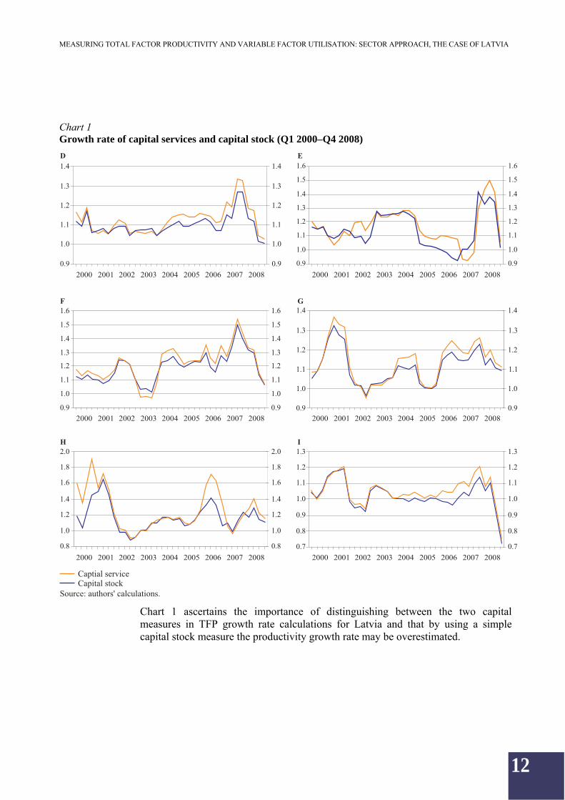
An important result of using a capital service rather than capital stock measure is that the service measure gives larger weights to assets with higher rental price in comparison with the asset price. Since the rental price depends on depreciation rates and changes in capital value, it is higher for assets with short service lives and a potential decline in price levels. This can explain higher weights given to intangible fixed assets, equipment and machinery in comparison with buildings and structures when obtaining the aggregated value of capital services. If the stocks of such assets grow faster than those of other asset types, the aggregate value of capital services will grow more rapidly than the aggregate value of capital stock, showing that the estimate based on the capital stock measure may overvalue the TFP growth over the respective period.

In the present study, four types of assets are distinguished: 1) intangible fixed assets, 2) buildings (dwellings are excluded), structures and cultivated assets, 3) machinery and equipment, and 4) other assets and inventories. To calculate the capital service measure, geometric depreciation of assets is assumed. More detailed information about investment series, price indexes, depreciation rates used in the calculation of aggregate capital service growth series, assumptions, and data sources is presented in Appendix 2.

The year-on-year comparison of obtained capital growth rates for Latvia calculated using capital stock price weights and rental price weights shows that when the rental price weights are used the growth of capital stock is faster (see Chart 1).

12


Chart 1 Growth rate of capital services and capital stock (Q1 2000–Q4 2008)

Chart 1 ascertains the importance of distinguishing between the two capital measures in TFP growth rate calculations for Latvia and that by using a simple capital stock measure the productivity growth rate may be overestimated.

13


3. TFP ESTIMATION RESULTS

In order to explore if the assumption of variable factor utilisation intensity improves the estimation of TFP growth in different sectors of the Latvian economy, regression equation [1.8] is obtained using the two-stage least squares method (2SLS) and the resulting TFP growth rate is compared with the estimation results obtained using the Solow residual approach. Since the authors' intention is to clear the TFP estimate from the effects of demand shocks, the set of instruments4 used includes the following variables: the world and foreign demand, domestic effective demand, fuel price index, consumer price index, nominal effective exchange rate, compensation per employee, and output gap. The precise list of instruments used in equations for different sectors is showed in Table 2.

Table 2 Instruments used in TFP growth calculation by sector of economy

Sec-tor

Period Growth rate Level

D t, t – 1 Foreign demand, world demand, real effective exchange rate

Output gap

E t, t – 1 Domestic effective demand, fuel price index, export, consumer price index

Output gap

F t, t – 1 Nominal effective exchange rate, compensation per employee, gross investment, consumer price index

Output gap

G t, t – 1 Nominal effective exchange rate, labour demand Output gap, unemployment rate

H t, t – 1 Compensation per employee, nominal effective exchange rate, consumer price index

Output gap

I t, t – 1 Trade turnover, compensation per employee, nominal effective exchange rate, world demand, fuel price

Output gap

By applying instrumental variables, it should be made sure that the chosen instrument satisfies two conditions: it must correlate with included variables and be orthogonal to the error process. The orthogonality condition can be verified by the Sargan test, which is a special case of Hansen's J test under the assumption of conditional homoskedasticity. The Sargan's statistic has an nRu

2 form and can be calculated by regressing the instrumental equation's residual (error) series upon all instruments (both the included exogenous variables and instruments). The nRu

2 of this regression (n is the number of observations) will have a χ2

L – K distribution (number of instruments L, number of parameters K). Its degrees of freedom are equal to the number of overidentifying restrictions and under the null hypothesis all instruments are orthogonal to the error.(26)

4 Variables that are correlated with input growth, but not with technology.

14


Results by sector

The results of above specified regression equation for six sectors of the Latvian economy are presented in Table 3.

The probability values obtained by the Sargan test for all sectors are higher than 0.3 and thereby confirm the orthogonality condition for instrumental variables used in the estimation. Constant c shows the fixed part of TFP growth rate of all sectors. The sign of the constant is positive for all sectors, yet their values are not significantly different from zero. The value of return to scale parameter γ is not statistically different from 1 for all sectors.

Table 3 TFP estimation results

Sector Variables Coefficient Standard. error Sargan test c 0.004 0.003 0.914 0.158***

H usual. /H actual growth rate, b1 0.316 0.111*** M/K growth rate, b2 0.359 0.048***

D

I/K growth rate, b3 –0.035 0.012***

0.577

c 0.002 0.005 1.056 0.210***

H usual. /H actual growth rate, b1 0.223 0.238 M/K growth rate, b2 0.704 0.124***

E

I/K growth rate, b3 0.028 0.023

0.306

c 0.001 0.012 0.818 0.230***

H usual. /H actual growth rate, b1 0.274 0.606 M/K growth rate, b2 0.089 0.211

F

I/K growth rate, b3 0.123 0.071*

0.430

c 0.005 0.006 0.928 0.199***

H usual. /H actual growth rate, b1 0.729 0.354** M/K growth rate, b2 0.326 0.084***

G

I/K growth rate, b3 0.018 0.032

0.433

c 0.002 0.004 0.977 0.089***

H usual. /H actual growth rate, b1 0.249 0.251 M/K growth rate, b2 0.448 0.047***

H

I/K growth rate, b3 –0.005 0.012

0.485

c 0.001 0.007 0.850 0.298***

H usual. /H actual growth rate, b1 0.518 0.272* M/K growth rate, b2 0.360 0.037***

I

I/K growth rate, b3 –0.073 0.032**

0.807

Note:*, **, and *** denote significance at the 10%, 5% and 1% level. Source: authors' calculations.

15


The effect of control for input utilisation is overall statistically significant; the joint restriction b1 = b2 = b3 = 0 is rejected for all sectors. The coefficients for the growth rate of actual to usual working hours ratio (b1) and growth rate of intermediate to capital service ratio (b2) are positive and in line with theoretical predictions. The estimated coefficients for the growth rate of investment to capital service ratio (b3) are negative in manufacturing (D), hotels and restaurants (H), and transport, storage and communication (I), showing that a short-run increase in investment to capital ratio will restrict the output growth due to costs of investment installation.

The comparison of the contribution of different utilisation components leads to a conclusion that the strongest effect from the increase in actual to usual working hours ratio (more intensive use of labour presented by coefficient b1) is present in wholesale and retail trade (G) as well as the transport, storage and communication (I) sector. It means that an increase in labour effort and capital service utilisation due to more intensive use of labour in these sectors will give a higher output growth measure compared with other sectors.

The response to a change in the growth rate of intermediate to capital service ratio is quite strong in all sectors (except the construction sector (F)), with the highest value of coefficient b2 for electricity, gas and water supply (E). Two possible theoretical explanations for the increase in the ratio of intermediate use to unit of capital can be given. First, capital is not fully employed and the increase in the volume of intermediate use results in a higher increase in the volume of output compared with other sectors. Second, this sector is more flexible to demand shocks and its production intensity can be easier adjusted by changing the volume of intermediate use. The first explanation might be more appropriate in the case of electricity, gas and water supply industry and manufacturing (E and D respectively), whereas the second one suits wholesale and retail trade (G) better.

The increase in the growth rate of investment to capital ratio has the strongest positive effect in the construction sector (F). Due to the strong increase in the demand for construction works, a more intensive use of capital in this sector might be showed, first, by a higher rate of capital depreciation and asset renovation, and, second, by a smaller effect of capital installation costs than in other sectors. A negative effect from the increase in the growth rate of investment to capital ratio is observed in sectors where investment installation costs are likely to be higher than in other sectors, e.g. equipment installation in manufacturing (D), long-term construction works in the hotel and restaurant sector (H), new facilities in the fast developing transport, storage and communication sector (I).

The findings in several studies (2; 8) suggest that by adjusting production factor utilisation intensity the TFP cyclical component can be reduced. This conclusion is confirmed also by the TFP estimates for Latvia (see Table 4). Incorporation into the model of a mechanism for the estimation of TFP utilisation intensity allows for decreasing fluctuations in the TFP measure and making it less output growth dependent.

16


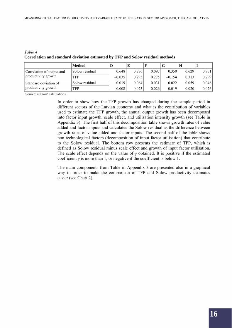
Table 4 Correlation and standard deviation estimated by TFP and Solow residual methods

Method D E F G H I

Solow residual 0.648 0.776 0.097 0.350 0.629 0.751Correlation of output and productivity growth TFP –0.035 0.293 0.275 –0.154 0.313 0.299

Solow residual 0.019 0.064 0.031 0.022 0.059 0.046Standard deviation of productivity growth TFP 0.008 0.023 0.026 0.019 0.020 0.026Source: authors' calculations.

In order to show how the TFP growth has changed during the sample period in different sectors of the Latvian economy and what is the contribution of variables used to estimate the TFP growth, the annual output growth has been decomposed into factor input growth, scale effect, and utilisation intensity growth (see Table in Appendix 3). The first half of this decomposition table shows growth rates of value added and factor inputs and calculates the Solow residual as the difference between growth rates of value added and factor inputs. The second half of the table shows non-technological factors (decomposition of input factor utilisation) that contribute to the Solow residual. The bottom row presents the estimate of TFP, which is defined as Solow residual minus scale effect and growth of input factor utilisation. The scale effect depends on the value of γ obtained. It is positive if the estimated coefficient γ is more than 1, or negative if the coefficient is below 1.

The main components from Table in Appendix 3 are presented also in a graphical way in order to make the comparison of TFP and Solow productivity estimates easier (see Chart 2).

17


Chart 2 Dynamics of value added, factor utilisation intensity, TFP and Solow residual (2000–2008) (year-on-year; %)

Manufacturing (D)

The results of TFP growth in the manufacturing sector of the Latvian economy show that during the analysed period the productivity of the sector was on an upward trend, increasing annually by 1.6% on average (see Table in Appendix 3 and Chart 2).

18


The control for utilisation intensity growth of input factors increases the estimated results of productivity growth for the sector in comparison with the Solow residual measure. The biggest share of utilisation measure in manufacturing is attributed to the change in the growth rate of intermediate to capital ratio. A negative growth of this ratio might be a sign of intensive capitalisation of the sector, with the capital growth exceeding the growth in intermediate consumption. It may, however, be also a sign of ineffective and incomplete use of capital. The changes in intermediate consumption, which also decrease the above ratio, usually present a reaction to a demand side shock in the economy.

From 2005 onwards, the growth rate of capital services exceeded that of intermediate inputs, reflecting larger investment in renovation and new production facilities and representing growing capitalisation of the sector. The particularly steep rise in capital services in 2007 can be explained by the construction of new production units (e.g. wood-based panel and cement industry facilities).

The effect of the global economic downturn and the subsequent drop in the internal and external demand for goods explain deceleration in the growth of intermediate consumption and a decrease in the ratio of actual to usual hours worked, which resulted in lower utilisation of sector's capital in 2007–2008. The control for separation of the TFP growth from its cyclical component with factor utilisation intensity variables leads to a conclusion that the sector productivity in 2008 remained positive as in the previous years despite the output growth in the sector dropping substantially.

Electricity, gas and water supply (E)

Since 1991, large reconstruction and renovation works have been carried out in Latvia to modernise and improve the operation of hydroelectric and heat power stations. Four hydroelectric units in 1991–1996 and two more later in 1999–2001 were renovated at the Pļaviņas hydroelectric power station, boosting the capacity and effectiveness of the station. In 2001, the reconstruction of the Ķegums hydroelectric power station was also accomplished. The first stage of renovation works of two heat power stations in Riga (Riga TEC I and TEC II) was finished in 2001 by constructing new facilities and installing up-to-date equipment in Riga TEC I. The second stage of renovation works at Riga TEC II started in 2004 and had been accomplished by the end of 2008. These reconstruction and renovation works improved the capacity and effectiveness of these heat power stations.

Due to renovation works above, the growth rate of capital exceeded that of intermediate inputs in the sector during the entire period, 2002–2004 and 2008 in particular (see Table in Appendix 3 and Chart 2). The replacement of capital is captured by the growth of intermediate to capital ratio in capital utilisation. Renovation of assets in the sector is a long-term process, and, compared with the growth of capital, it will not bring an immediate increase in the output growth. Consequently, the decrease in the capital utilisation intensity in the sector shows its capitalisation level. An additional strong impact on the decrease in input factor utilisation intensity was present in 2007 and 2008 due to decelerating growth rate of the ratio of actual to usual weekly working hours, which can be explained by the combination of a more effective use of human capital due to implementation of new

19


technology and a decrease in intensity of factor use due to weather conditions (warm winters).

The results of TFP growth show that from 2001 productivity of the sector increased and reached 3.1% in 2008. The average annual TFP growth in 2001–2008 was 1.6% (see Table in Appendix 3).

Construction (F)

Compared with other sectors, the construction sector of the Latvian economy recorded the sharpest output drop after the 1990s. An intense growth of the sector has been observed since 2002, with output growing by more above than 10% annually. The development of the financial sector, expanding financing facilities, and availability of credits gave a strong impulse for an exponential development of the construction sector starting with 2004.

After an economic downturn in the 1990s and a long period of downtime in the construction sector, substantial investment in capital assets was needed to boost sector's capacity. The growth of capital exceeded the growth of intermediate inputs during the entire period, except for 2003. This fact, similarly to the developments in sector E, is captured by the negative growth of intermediate to capital ratio and might be explained by capitalisation of the sector (see Table in Appendix 3). As the depreciation rate of capital assets was growing, the ratio of investment to capital also grew since 2002, which together with a positive sign of coefficient 3 shows an

increase in utilisation intensity of production factors.

A specific feature of the construction sector in comparison with other sectors of the Latvian economy is the strong negative correlation between the growth in labour factor inputs and the ratio of actual to usual working hours (see Table). Respectively, the more the labour force is employed, the lesser is the intensity of its use, which might be explained by the insufficient qualification of labour force in the sector.

Since the middle of 2007, when the price of a square meter of real estate reached the peak, the real estate market indicators were continuously falling. Slashed prices together with instability of the financial market substantially dampened the demand for real estate and confined the development of the construction industry. It is indicated by a decrease in the ratios of the three components, i.e. actual to usual working hours, investment to capital, and intermediate consumption to capital ratios.

The very fast development of industry notwithstanding, the productivity growth trend was volatile. The average annual TFP growth in 2001–2008 was only 0.3% (see Chart 2). Due to decreasing demand for construction works at the end of 2007, the effectiveness of factor use and productivity in construction improved in 2008, recording a 2.1% growth.

Wholesale and retail trade (G)

The development of wholesale and retail trade in Latvia was very much influenced by foreign investment in the development of distributing facilities, supermarket networks and shopping centres. A very intensive growth of shopping areas was

20


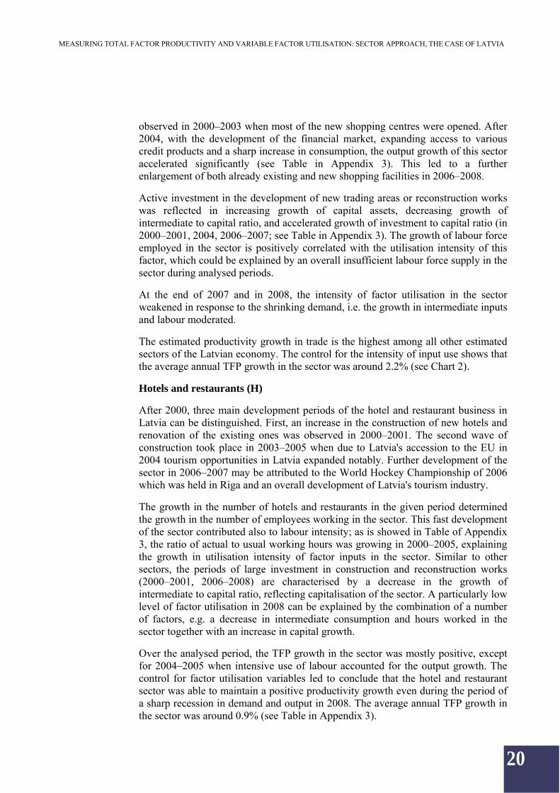
observed in 2000–2003 when most of the new shopping centres were opened. After 2004, with the development of the financial market, expanding access to various credit products and a sharp increase in consumption, the output growth of this sector accelerated significantly (see Table in Appendix 3). This led to a further enlargement of both already existing and new shopping facilities in 2006–2008.

Active investment in the development of new trading areas or reconstruction works was reflected in increasing growth of capital assets, decreasing growth of intermediate to capital ratio, and accelerated growth of investment to capital ratio (in 2000–2001, 2004, 2006–2007; see Table in Appendix 3). The growth of labour force employed in the sector is positively correlated with the utilisation intensity of this factor, which could be explained by an overall insufficient labour force supply in the sector during analysed periods.

At the end of 2007 and in 2008, the intensity of factor utilisation in the sector weakened in response to the shrinking demand, i.e. the growth in intermediate inputs and labour moderated.

The estimated productivity growth in trade is the highest among all other estimated sectors of the Latvian economy. The control for the intensity of input use shows that the average annual TFP growth in the sector was around 2.2% (see Chart 2).

Hotels and restaurants (H)

After 2000, three main development periods of the hotel and restaurant business in Latvia can be distinguished. First, an increase in the construction of new hotels and renovation of the existing ones was observed in 2000–2001. The second wave of construction took place in 2003–2005 when due to Latvia's accession to the EU in 2004 tourism opportunities in Latvia expanded notably. Further development of the sector in 2006–2007 may be attributed to the World Hockey Championship of 2006 which was held in Riga and an overall development of Latvia's tourism industry.

The growth in the number of hotels and restaurants in the given period determined the growth in the number of employees working in the sector. This fast development of the sector contributed also to labour intensity; as is showed in Table of Appendix 3, the ratio of actual to usual working hours was growing in 2000–2005, explaining the growth in utilisation intensity of factor inputs in the sector. Similar to other sectors, the periods of large investment in construction and reconstruction works (2000–2001, 2006–2008) are characterised by a decrease in the growth of intermediate to capital ratio, reflecting capitalisation of the sector. A particularly low level of factor utilisation in 2008 can be explained by the combination of a number of factors, e.g. a decrease in intermediate consumption and hours worked in the sector together with an increase in capital growth.

Over the analysed period, the TFP growth in the sector was mostly positive, except for 2004–2005 when intensive use of labour accounted for the output growth. The control for factor utilisation variables led to conclude that the hotel and restaurant sector was able to maintain a positive productivity growth even during the period of a sharp recession in demand and output in 2008. The average annual TFP growth in the sector was around 0.9% (see Table in Appendix 3).

21


Transport, storage and communication (I)

The transport, storage and communication sector of Latvia was continuously evolving, with mostly positive rates of capital and labour input growth during the analysed period. Much renovation and restructuring works were carried out within each sub-sector, e.g. communication industry developed rapidly, investment in airport cargo and passenger transportation service development was solid, transportation of goods via railroad and pipelines increased, port services expanded, etc.

Despite overall large investment in the sector, the control for utilisation intensity of factor inputs detects a period of a very intensive use of capital and labour during 2000–2005 (see Chart 2). The growth in both actual to usual working hour ratio and intermediate to capital ratio was positive and significant and pointed to a strong demand for input factors due to the growing freight turnover.

The productivity growth during 2001–2003 was negative, indicating that the output growth in the sector had been possible mainly due to the intensive use of capital and labour. Starting with 2004, the TFP growth accelerated and the use of labour and capital factors became less intensive. The average annual TFP growth in the sector was about 0.1% (see Table in Appendix 3).

In 2008, the transport, storage and communication was the only sector which did not record negative growth of intermediate consumption in response to demand shock. Lower labour factor utilisation rate together with a slight increase in intermediate consumption and deceleration in capital growth ensured the lowest decrease in utilisation of inputs in comparison with other sectors.

22


CONCLUSIONS

The aim of the paper is to estimate changes in the growth rate of TFP for the main sectors of the Latvian economy by applying a model accounting for utilisation intensity of variable production factors. The results of the paper show that the control for factor utilisation intensity plays a significant role in explaining the growth in goods and services output.

In order to generate accurate measures for TFP estimation, the capital and labour time series have been adjusted for their quality and structural changes. This adjustment is based on corresponding wages of three different levels of education for labour force and capital rental prices for four types of fixed assets. The year-on-year comparison of capital growth rates of the Latvian economy calculated from the asset price weights and rental price weights shows that the fixed asset growth calculated on the basis of rental price weights is faster. This confirms the importance of distinguishing between two capital measures for TFP calculations and suggests that overestimation of productivity growth rate is possible if the simple capital stock measure is used.

A single regression equation for TFP estimation is derived from the theoretical cost-minimisation problem of a firm. An important supplement to the regular production function regression is the factor utilisation intensity part, which helps to control for intensity of production factor utilisation. Since utilisation intensity is an unobservable variable, three proxy indicators are used to define utilisation intensity of input factors: growth in the ratio of actual to usual weekly working hours, in the ratio of intermediate consumption to capital, and in the ratio of investment to capital.

The comparison of effects of input factor utilisation intensity for different sectors of the Latvian economy shows that the strongest effect from an increase in ratio of actual to usual working hours is present in wholesale and retail trade (G), and in the transport, storage and communication sector (I). Almost all sectors strongly react to a change in the growth rate of intermediate to capital ratio, which might be explained by not fully employed capital in the case of electricity, water and gas supply (E) and manufacturing sectors (D), and higher resilience to demand shocks in the case of wholesale and retail trade (G), transport, storage and communication (I), and hotels and restaurants (H). The increase in the growth of investment to capital ratio had the strongest positive effect in the construction sector (F), which might be explained by a higher depreciation rate of capital and asset renovations and, possibly, by smaller impact from capital installation costs in comparison with other sectors. A negative effect of the increase in growth rate of investment to capital ratio is recorded for sectors where investment installation costs could be higher, e.g. installation of equipment in manufacturing (D), long-term construction works in the hotel and restaurant sector (H), building of new facilities in the fast developing transport, storage and communication sector (I).

The results of TFP estimation for Latvia are in line with conclusions of several studies (2; 8), showing that by adjusting for variable utilisation intensity in the model the cyclical component of TFP growth and volatility can be reduced. Fluctuations in the TFP measure decrease and the TFP measure becomes less output growth dependent.

23


The comparison of the growth rate of the Solow residual and TFP growth, two productivity measures, shows that the control for utilisation intensity of production factors gives higher and stabler productivity estimates in the case of manufacturing (D), electricity, gas and water supply (E), hotels and restaurants (H), and wholesale and retail trade (G). On the other hand, the productivity growth in construction (F) is volatile, with a very low productivity growth during the analysed period on average. The obtained TFP growth in the transport, storage and communication sector (I) suggests a period of very intense use of factor inputs from 2001 to 2005 (in 2001–2003, the average annual productivity growth was negative, turning positive thereafter).

24


APPENDICES

Appendix 1 MEASURING AGGREGATE PRODUCTIVITY GROWTH

The production function in logarithm notation

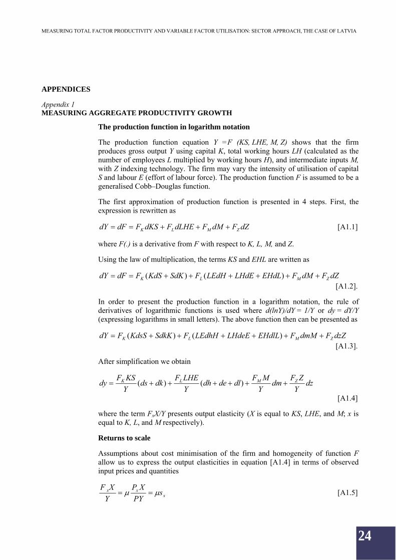
The production function equation Y =F (KS, LHE, M, Z) shows that the firm produces gross output Y using capital K, total working hours LH (calculated as the number of employees L multiplied by working hours H), and intermediate inputs M, with Z indexing technology. The firm may vary the intensity of utilisation of capital S and labour E (effort of labour force). The production function F is assumed to be a generalised Cobb–Douglas function.

The first approximation of production function is presented in 4 steps. First, the expression is rewritten as

dZFdMFdLHEFdKSFdFdY ZMLK [A1.1]

where F(.) is a derivative from F with respect to K, L, M, and Z.

Using the law of multiplication, the terms KS and EHL are written as

dZFdMFEHdLLHdELEdHFSdKKdSFdFdY ZMLK )()( [A1.2].

In order to present the production function in a logarithm notation, the rule of derivatives of logarithmic functions is used where d(lnY)/dY = 1/Y or dy = dY/Y (expressing logarithms in small letters). The above function then can be presented as

dzZFdmMFEHdlLLHdeELEdhHFSdkKKdsSFdY ZMLK )()( [A1.3].

After simplification we obtain

dzY

ZFdm

Y

MFdldedh

Y

LHEFdkds

Y

KSFdy ZMLK )()(

[A1.4]

where the term FxX/Y presents output elasticity (X is equal to KS, LHE, and M; x is equal to K, L, and M respectively).

Returns to scale

Assumptions about cost minimisation of the firm and homogeneity of function F allow us to express the output elasticities in equation [A1.4] in terms of observed input prices and quantities

xxx s

PY

XP

Y

XF [A1.5]

25


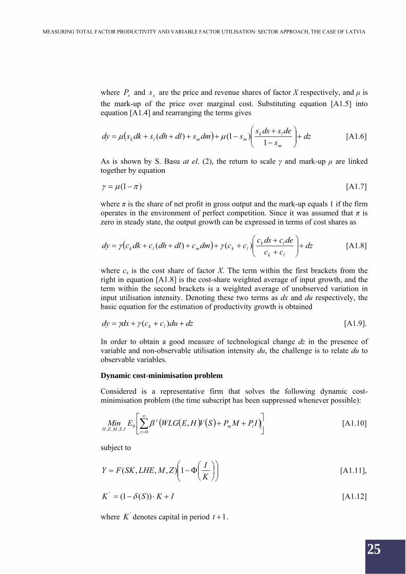
where xP and xs are the price and revenue shares of factor X respectively, and μ is

the mark-up of the price over marginal cost. Substituting equation [A1.5] into equation [A1.4] and rearranging the terms gives

dzs

desdsssdmsdldhsdksdy

m

lkmmlk

1

)1()( [A1.6]

As is shown by S. Basu at el. (2), the return to scale γ and mark-up μ are linked together by equation

)1( [A1.7]

where π is the share of net profit in gross output and the mark-up equals 1 if the firm operates in the environment of perfect competition. Since it was assumed that π is zero in steady state, the output growth can be expressed in terms of cost shares as

dzcc

decdscccdmcdldhcdkcdy

lk

lklkmlk

)()( [A1.8]

where cx is the cost share of factor X. The term within the first brackets from the right in equation [A1.8] is the cost-share weighted average of input growth, and the term within the second brackets is a weighted average of unobserved variation in input utilisation intensity. Denoting these two terms as dx and du respectively, the basic equation for the estimation of productivity growth is obtained

dzduccdxdy lk )( [A1.9].

In order to obtain a good measure of technological change dz in the presence of variable and non-observable utilisation intensity du, the challenge is to relate du to observable variables.

Dynamic cost-minimisation problem

Considered is a representative firm that solves the following dynamic cost-minimisation problem (the time subscript has been suppressed whenever possible):

00

,,,,,

IPMPSVHEWLGEMin imISMEH

[A1.10]

subject to

K

IZMLHESKFY 1),,,( [A1.11],

IKSK ))(1(' [A1.12]

where 'K denotes capital in period 1t .

26


The first-order conditions for the minimisation problem are given in equations [A1.13]–[A1.17] where λ is the Lagrange multiplier for gross output and q is the Lagrange multiplier for capital formation function. The expression (1 – Φ(I/K)) is substituted by Y/F from equation [A1.11].

:)(H )(),(),,,( SVHEWLGF

YZMLHESKELF HL [A1.13],

:)(E )(),(),,,( SVHEWLGF

YZMLHESKHLF EL [A1.14],

:)(M mM PF

YZMLHESKF ),,,( [A1.15],

:)(S KSqSVHEWLGF

YZMLHESKKFK )(')('),(),,,( [A1.16],

:)(I qK

YPI

1

' [A1.17].

In order to express labour effort intensity in terms of observable variables, the first order condition for effort intensity (equation [A1.14]) and for working hours (equation [A1.13]) is used. By combining these expressions, it is obtained that elasticity of labour costs with respect to working hours is equal to elasticity of labour costs with respect to effort intensity:

),(),( HEHGHEEG HE [A1.18]

and could be written as

)(HEE [A1.19].

Thus, the unobservable labour utilisation (effort) intensity can be expressed as a function of the observed number of hours per worker.

Log-linearising of the above expression gives

);(')(

1)(ln HE

HEHEdde dH

HHddh

1ln

dhdhHE

HHEde

)(

)(' [A1.20]

where ζ is the elasticity of effort with respect to hours.

Capital utilisation intensity

In order to express capital utilisation in terms of observable variables, several first order conditions derived above are combined. First, in equation [A1.16] of the first

27


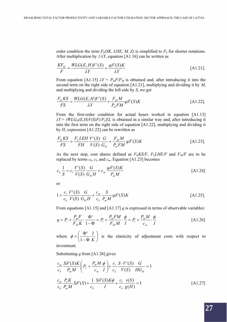
order condition the term Fk(SK, LHE, M, Z) is simplified to Fk for shorter notations. After multiplication by 1/λY, equation [A1.16] can be written as

Y

KSq

Y

SVHEWLG

F

KFK

)(')('),(

[A1.21].

From equation [A1.15] λY = PmF/FM is obtained and, after introducing it into the second term on the right side of equation [A1.21], multiplying and dividing it by M, and multiplying and dividing the left side by S, we get

KSqFMP

MF

Y

SVHEWLG

FS

KSF

m

MK )(')('),(

[A1.22].

From the first-order condition for actual hours worked in equation [A1.13] λY = (WLGH(E,H)V(S)F)/FLEL is obtained in a similar way and, after introducing it into the first term on the right side of equation [A1.22], multiplying and dividing it by H, expression [A1.22] can be rewritten as

KSqFMP

MF

G

G

SV

SV

FH

LEHF

FS

KSF

m

M

H

LK )(')(

)(' [A1.23].

As the next step, cost shares defined as FKKS/F, FLLHE/F and FM/F are to be replaced by terms ck, cl, and cm. Equation [A1.23] becomes

MP

KSqc

HG

G

SV

SVc

Sc

mm

Hlk

)('

)(

)('1 [A1.24]

or

KSqMP

S

c

c

HG

G

SV

SV

c

c

mk

m

Hk

l )(')(

)('1 [A1.25].

From equations [A1.15] and [A1.17] q is expressed in terms of observable variables:

Ic

MPP

IMF

FMPP

KF

FPPq

m

mi

M

mi

M

mi

1

' [A1.26]

where

K

I

1

' is the elasticity of adjustment costs with respect to

investment.

Substituting q from [A1.26] gives

1)(

)(')('

Hk

l

m

mI

mk

m

HG

G

SV

SVS

c

c

Ic

MPP

MP

KSS

c

c

1)(

)()('1)('

Hg

Sv

c

c

I

KSS

cSS

MP

KP

c

c

k

l

km

I

k

m [A1.27]

28


where v(S) = SV'(S)/V(S) is the elasticity of shift premium with respect to utilisation intensity and g(H) = GHH/G is the elasticity of wage rate with respect to hours worked.

Before log-linearising equation [A1.27], following S. Basu and M. S. Kimball (3) and C. Groth, S. Nunez and S. Srinivasan (8), the following steady-state elasticities are defined:

)('

)(''

1)('

)(''1

ln

))('ln(

S

SSS

S

S

Sd

Sd

[A1.28],

)(

)('

1)(

)('1

ln

))(ln(

Sv

SvSS

Sv

Sv

Sd

Svdv

[A1.29],

)(

)('

1)(

)('1

ln

))(ln(

Hg

HgHH

Hg

Hg

Hd

Sgd

[A1.30]

where Δ is the elasticity of marginal depreciation with respect to capital utilisation intensity, v is the rate at which elasticity of labour costs (shift premium) increases with respect to capital utilisation intensity, and g is the rate at which elasticity of labour costs increases with respect to growth of hours worked.

Also, the shares of higher utilisation intensity costs due to faster wear out of production factors and the inclusion of shift premium are defined:

I

KSS

ck

)('1 [A1.31],

MP

KPSS

c

c

m

I

k

m )(' [A1.32],

)(

)(

Hg

Sv

c

c

k

l [A1.33].

Log-linearising equation [A1.27] using the rules of log-linearisation and above definitions, the steady state equation is derived:

dmdpdkdpds

S

S

S

Sds

MP

KPSS

c

cmI

m

I

k

m

)(''

)("1

)('1

+

)(

/

)'/(

'

)(''

)("1

)('1dkdi

KI

KIdidkds

S

S

S

Sds

I

KSS

ck

+

dh

Hg

H

H

Hgds

Sv

S

S

Sv

Hg

Sv

c

c

k

l

)('

)('

)('

)('1

)(

)(;

29


);()('

10 dhvdsdkdiK

Idsdsdmdpdkdpdsds mI

dsdmdpdkdp mI ))(1(0 –

)()('

1 dhvdsdkdiK

I

[A1.34].

Expressing ds from equation [A1.34], the result is as follows:

dhdkdiK

Idkdpdmdp

vds Im

)(

'1)((

))(1(

1

and applying that 1

))(1(()1)(1(

1dkdpdmdp

vds Im

+

dhdkdiK

I

)(

'1 [A1.35].

Euler equation for capital

The assumption of the specification of cost-minimisation problem about the installation of new capital being costly suggests that output elasticities are not equal to the respective cost shares. It could be explained by the fact that in line with this specification the firm produces two types of commodities: the output commodity and the installation service of new capital.

The authors of this paper follow the derivation of Euler equation for capital by C. Groth, S. Nunez and S. Srinivasan (8) to define the output elasticity of capital, which will depend on both income share and adjustment costs.

The Euler equation for above specified cost-minimisation problem can be written as

11

2)1(

1

'

qq

K

IY

F

YSFk

[A1.36].

Interpreting λ as marginal costs and assuming that μ is the mark-up over marginal costs, the steady state elasticity with respect to capital from equation [A1.36] can be showed as5

kkk cs

pY

Krq

F

SKF )( [A1.37].

5 For detailed analysis see (8).

30


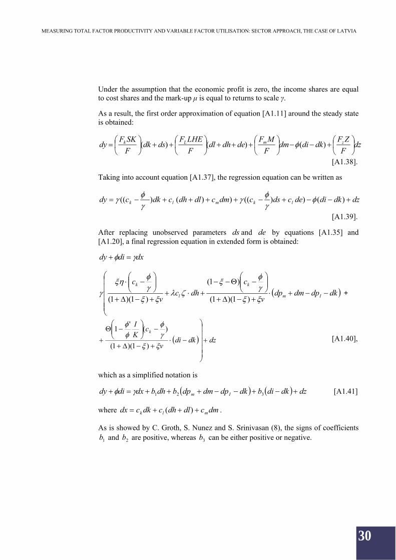
Under the assumption that the economic profit is zero, the income shares are equal to cost shares and the mark-up μ is equal to returns to scale γ.

As a result, the first order approximation of equation [A1.11] around the steady state is obtained:

dzF

ZFdkdidm

F

MFdedhdl

F

LHEFdsdk

F

SKFdy zmLk

)()()(

[A1.38].

Taking into account equation [A1.37], the regression equation can be written as

dzdkdidecdscdmcdldhcdkcdy lkmlk )())(())()((

[A1.39].

After replacing unobserved parameters ds and de by equations [A1.35] and [A1.20], a final regression equation in extended form is obtained:

dxdidy

dkdpdmdpv

c

dhcv

c

Im

k

l

k

)1)(1(

)1(

)1)(1( +

dzdkdiv

cK

Ik

)1)(1(

)('

1 [A1.40],

which as a simplified notation is

dzdkdibdkdpdmdpbdhbdxdidy Im 321 [A1.41]

where dmcdldhcdkcdx mlk )( .

As is showed by C. Groth, S. Nunez and S. Srinivasan (8), the signs of coefficients

1b and 2b are positive, whereas 3b can be either positive or negative.

31


Appendix 2 FACTOR INPUTS: DATA AND METHODS USED

This appendix describes data and methods used to construct quality adjusted labour force and capital service time series.

Labour inputs

The source of employment statistics is labour force surveys (LFS) provided by the Central Statistical Bureau of Latvia. Time series are available starting from the first quarter of 1998. Seasonally adjusted quarterly data on total sector employment are used. Data on the structure of labour force by level of education and by sector of the economy are available only on an annual basis. To produce quarterly time series of three levels of education for every sector, it was assumed that the structure of education in all sectors remains unchanged during the year. Since only average annual wages of the total economy for defined levels of education are available, the aggregate labour input growth for each sector was calculated using quarterly unchanged wage structure.

Since all the structural information is annual, the difference between the aggregate usual and quality adjusted measure of labour inputs is observed only for the first quarter. This limits the level of obtained quality adjusted labour force growth. For further studies, more detailed information would be preferable.

Capital services

Following the specification of the model presented by N. Oulton (18) and N. Oulton and S. Srinivasan (20), equations to construct the volume index of capital services are as follows:

1,)1( tiiitit AIA [A2.1],

1, tiit AK [A2.2],

Ati

Ait

Aiti

Atitt

Kit pppprTp 1,1, [A2.3],

m

i itAti

Ait

Aiti

Atitt

m

i itKitt KpppprTKp

1 1,1,1 [A2.4],

1,11 /ln/ln tiit

m

i ittt KKwKK [A2.5],

,2/)( 1, tiitit www

m

i itKit

itKit

itKp

Kpw

1

, mi ,...,1 [A2.6]

where m is the number of asset types, Ait is the real stock of the ith type of assets at the end of period t, Iit is the real gross investment in the asset of type i during period t, δi is the geometric rate of depreciation of the asset of type I, Kit is the real capital service from the asset of type i at the end of period t, pit

K is the rental price of a new asset of type i payable at the end of period t, pit

A is the corresponding price of the

32


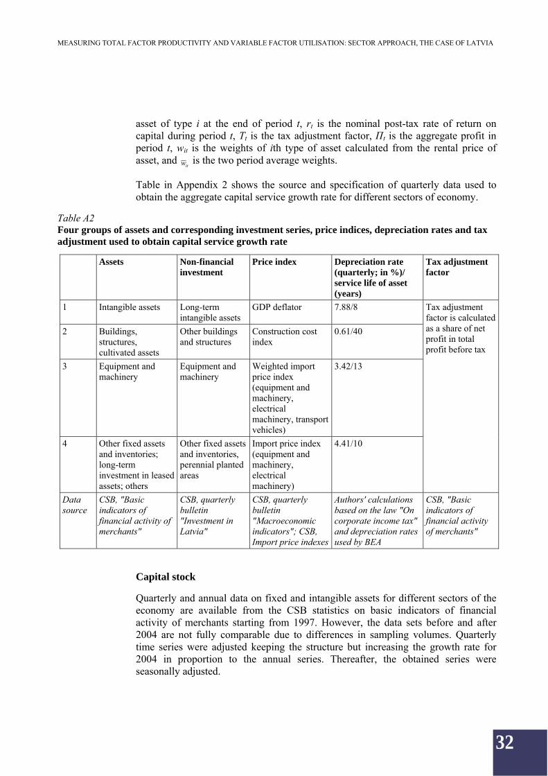
asset of type i at the end of period t, rt is the nominal post-tax rate of return on capital during period t, Tt is the tax adjustment factor, Πt is the aggregate profit in period t, wit is the weights of ith type of asset calculated from the rental price of asset, and

itw is the two period average weights.

Table in Appendix 2 shows the source and specification of quarterly data used to obtain the aggregate capital service growth rate for different sectors of economy.

Table A2 Four groups of assets and corresponding investment series, price indices, depreciation rates and tax adjustment used to obtain capital service growth rate

Assets Non-financial investment

Price index Depreciation rate (quarterly; in %)/ service life of asset (years)

Tax adjustment factor

1 Intangible assets Long-term intangible assets

GDP deflator 7.88/8

2 Buildings, structures, cultivated assets

Other buildings and structures

Construction cost index

0.61/40

3 Equipment and machinery

Equipment and machinery

Weighted import price index (equipment and machinery, electrical machinery, transport vehicles)

3.42/13

4 Other fixed assets and inventories; long-term investment in leased assets; others

Other fixed assets and inventories, perennial planted areas

Import price index (equipment and machinery, electrical machinery)

4.41/10

Tax adjustment factor is calculated as a share of net profit in total profit before tax

Data source

CSB, "Basic indicators of financial activity of merchants"

CSB, quarterly bulletin "Investment in Latvia"

CSB, quarterly bulletin "Macroeconomic indicators"; CSB, Import price indexes

Authors' calculations based on the law "On corporate income tax" and depreciation rates used by BEA

CSB, "Basic indicators of financial activity of merchants"

Capital stock

Quarterly and annual data on fixed and intangible assets for different sectors of the economy are available from the CSB statistics on basic indicators of financial activity of merchants starting from 1997. However, the data sets before and after 2004 are not fully comparable due to differences in sampling volumes. Quarterly time series were adjusted keeping the structure but increasing the growth rate for 2004 in proportion to the annual series. Thereafter, the obtained series were seasonally adjusted.

33


Data on the structure of fixed assets are available only on an annual basis. Therefore, in calculating fixed asset time series for three groups of assets, the aggregate seasonally adjusted quarterly series of fixed assets for each sector were divided on the basis of unchanged fixed asset structure during the year.

Investment

Aggregate quarterly investment series and their structure are available starting from 1997 from the CSB quarterly bulletin on investment in Latvia. In 2005, the sampling volume was changed and formally the data of two periods can not be compared. To overcome this complication, the total investment volume was increased proportionally (keeping the structure of quarterly series) so that the fixed asset series, which could be obtained from investment data and depreciation rates, are similar to the adjusted data on capital stock. Thereafter, according to the initial structure of investment series, each series group was adjusted proportionally.

Price indexes

In order to operate with the real values of capital and investment series, corresponding price indexes were chosen (see Table in Appendix 1). Since a considerable part of equipment and machinery is imported, the price index for this group is calculated as the weighted import price index for equipment and machinery, electrical machinery, and transport vehicles. The price index for buildings and structures is straightforward – it is the construction cost index. For the other two groups of investment, it was more difficult to find a relevant price index, so the GDP deflator was chosen as deflator for intangible assets and the import price index for equipment and machinery, electrical machinery became a deflator for other assets. Price indexes do not differ among sectors due to the lack of data. All price indexes have been seasonally adjusted and set to 1 in the first quarter of 1998.

Depreciation

Depreciation rates used in accounting in Latvia are provided in the law of the Republic of Latvia "On Corporate Income Tax". These rates are based on the double declining balance method

6 adopting a straight-line depreciation pattern. The

geometric depreciation calculation method fits the data on asset prices well (10; 17), and it is frequently used in the studies on productivity growth (18; 19; 20; 7; 8; 2; 3). As is showed by B. M. Fraumeni (6), it is possible to recalculate the depreciation rate of straight-line pattern into geometric depreciation rate by dividing the corresponding double declining balance rate by the estimated service life of the asset. In this study, the declining balance rates applied by the BEA are used.

Table in Appendix 1 shows recalculated quarterly depreciation rates for Latvia. The equipment and machinery asset group is not separately specified in the law, therefore depreciation rates from BEA tables are used in this paper. Since intangible

6 Depreciation is equal to TR / where T is average asset service live and R is estimated

declining-balance rate (R = 2 in the case of double declining balance method). Several empirical researches show that the declining balance rate for different asset groups differs from 2 (see (6) for the estimated declining balance rates adopted by the BEA).

34


asset group is very complex, a specific depreciation rate is not available and was calculated from capital and investment data of intangible assets for the total economy.

Tax adjustment factor

The tax adjustment factor is calculated as an inverse share of net profit in total profit before tax. The data source is CSB statistics on basic indicators of financial activity of merchants. The quarterly data are adjusted to fit total annual data, keeping their structure and sign. The obtained series of tax rates for every sector were adjusted using the HP filter with lambda value which is equal to 2.

Capital service price

To derive capital service prices, first equation [A2.4] is used to calculate the post-tax rate of return and, after substituting the obtained value into equation [A2.3)], to calculate the capital service price. Further on, in order to obtain the aggregate capital service growth rate, prices are used as weights for each asset type.

35


Appendix 3 OUTPUT GROWTH DECOMPOSITION

This appendix shows how the annual output growth is decomposed into factor inputs, scale effect, and utilisation intensity of inputs for six sectors of the Latvian economy. The first half of Table in Appendix 3 shows the growth rates of value added and factor inputs and calculates the Solow residual as the growth rate of value added minus factor inputs. The second half of the Table shows non-technological factors (factor utilisation intensity) that contribute to the Solow residual. The bottom row presents the estimate of TFP growth, which is defined as Solow residual minus scale effect and growth of input factor utilisation intensity.

Table A3 Output growth decomposition by sector of economy (2000–2008)

2000 2001 2002 2003 2004 2005 2006 2007 2008 Manufacturing (D) Output growth 3.1 9.6 8.0 5.9 6.1 5.2 5.9 1.4 –6.0– Intermediate consumption growth 0.5 5.6 4.8 3.4 3.4 3.4 3.5 1.0 –2.8

= Value added growth 2.7 4.0 3.3 2.5 2.6 1.8 2.4 0.4 –3.3 – Input growth 3.9 1.9 3.0 1.7 3.0 3.6 4.7 8.2 3.4 Capital growth 4.0 2.2 2.7 1.8 3.6 4.4 3.9 7.7 3.2 Labour growth –0.1 –0.3 0.3 –0.1 –0.6 –0.8 0.8 0.4 0.2

= Solow residual –1.2 2.2 0.2 0.8 –0.4 –1.8 –2.3 –7.7 –6.7 + Scale effect –0.4 –0.6 –0.7 –0.4 –0.6 –0.6 –0.7 –0.8 –0.1 + Utilisation intensity of inputs –3.1 2.5 –2.3 –0.4 –2.3 –2.0 –2.1 –8.6 –8.3 Δh 1.0 1.1 –0.3 –0.6 –0.1 0.7 0.7 –0.7 –3.3 Δm-Δk –4.4 1.0 –0.1 0.1 –2.0 –2.9 –2.3 –8.4 –5.5 Δi-Δk 0.3 0.3 –1.8 0.1 –0.2 0.3 –0.5 0.6 0.5

+ TFP growth 2.3 0.3 3.2 1.7 2.5 0.9 0.5 1.5 1.7

Electricity, gas and water supply (E) Output growth –15.9 5.4 4.7 4.2 4.7 3.0 3.9 1.5 –2.2– Intermediate consumption growth –2.1 1.4 1.2 1.4 1.4 0.6 0.9 0.0 –0.1

= Value added growth –13.8 4.0 3.5 2.8 3.3 2.5 3.0 1.5 –2.0 – Input growth 8.8 5.2 11.7 14.0 16.5 4.6 5.5 1.8 20.0 Capital growth 9.3 5.3 10.8 14.6 15.1 5.8 5.5 2.0 20.0 Labour growth –0.5 –0.1 0.9 –0.6 1.4 –1.2 0.0 –0.1 0.0

= Solow residual –22.6 –1.2 –8.2 –11.2 –13.2 –2.1 –2.5 –0.3 –22.1 + Scale effect 0.4 0.4 0.7 0.9 1.0 0.3 0.4 0.1 1.1 + Utilisation intensity of inputs –15.2 –1.6 –10.2 –13.3 –13.9 –4.8 –4.1 –4.9 –26.3 Δh 0.8 0.7 0.3 0.3 –0.3 0.4 –0.1 –1.5 –2.6 Δm-Δk –15.7 –2.7 –9.4 –13.2 –13.7 –5.3 –4.1 –3.5 –23.9 Δi-Δk –0.3 0.4 –1.1 –0.4 0.1 0.2 0.2 0.1 0.2

+ TFP growth –7.3 0.1 1.3 1.2 –0.4 2.3 1.2 4.2 3.1

36


2000 2001 2002 2003 2004 2005 2006 2007 2008 Construction (F) Output growth 11.7 6.1 9.1 12.7 12.7 14.6 19.8 10.6 –3.2– Intermediate consumption growth 5.5 3.9 6.2 8.5 8.2 9.5 12.8 6.1 –2.3

= Value added growth 6.2 2.2 2.9 4.2 4.5 5.1 7.0 4.4 –0.9 – Input growth 1.1 5.1 1.5 4.2 6.2 4.8 7.2 9.2 3.2 Capital growth 2.5 2.2 3.3 0.1 4.6 3.6 4.6 6.0 3.4 Labour growth –1.3 3.0 –1.8 4.1 1.6 1.2 2.6 3.2 –0.2

= Solow residual 5.0 –2.9 1.4 0.0 –1.7 0.3 –0.2 –4.8 –4.1 + Scale effect –1.3 –1.7 –1.4 –2.3 –2.6 –2.6 –3.7 –2.8 –0.2 + Utilisation intensity of inputs 2.1 –0.8 1.4 1.5 0 5.1 3.8 –2.2 –5.7 Δh 0.8 1.6 1.7 –1.7 –0.6 0.6 0.3 –0.1 –0.7 Δm-Δk –0.5 –0.6 –0.9 1.1 –1.3 –0.6 –0.7 –2.3 –2.1 Δi-Δk 1.8 –1.8 0.6 2.1 2.0 5.1 4.2 0.3 –3.0

+ TFP growth 4.4 –0.5 1.4 0.8 0.9 –2.2 –0.5 0.2 2.1

Wholesale and retail trade (G) Output growth 4.6 9.4 11.1 9.3 11.4 14.9 18.5 13.0 –9.2– Intermediate consumption growth 0.9 5.5 6.2 5.2 6.1 6.5 10.5 6.2 –5.2

= Value added growth 3.7 3.9 4.8 4.1 5.2 8.4 7.9 6.7 –3.9 – Input growth 5.1 8.8 –0.6 1.2 4.9 0.8 8.2 7.2 4.8 Capital growth 4.6 8.4 0.2 1.2 5.2 0.7 6.7 6.7 4.7 Labour growth 0.5 0.5 –0.7 0.0 –0.3 0.1 1.6 0.6 0.1

= Solow residual –1.4 –5.0 5.4 3.0 0.3 7.6 –0.3 –0.5 –8.7 + Scale effect –0.4 –1.0 –0.4 –0.5 –0.8 –0.5 –1.3 –1.0 0.0 + Utilisation intensity of inputs –2.2 –3.8 2.9 2.4 –2.9 3.8 0.3 –2.9 –11.0 Δh 1.7 1.0 –0.2 0.1 –1.7 1.0 –0.4 –0.2 –2.9 Δm-Δk –4.0 –5.0 3.7 2.1 –1.4 3.3 –0.1 –2.8 –7.9 Δi-Δk 0.1 0.2 –0.5 0.2 0.1 –0.5 0.8 0.1 –0.3

+ TFP growth 1.4 –0.1 2.8 1.0 4.0 4.3 0.7 3.3 2.3 Hotels and restaurants (H) Output growth 5.1 12.6 0.8 22.6 14.6 12.6 17.2 2.1 –16.8– Intermediate consumption growth 0.7 5.8 0.0 9.8 6.6 5.9 8.1 –0.3 –8.6

= Value added growth 4.4 6.9 0.8 12.8 8.0 6.7 9.1 2.4 –8.2 – Input growth 26.9 20.0 –1.8 2.6 6.1 7.3 22.8 3.5 10.2 Capital growth 25.4 19.3 –1.7 2.4 6.7 5.7 21.8 3.6 10.9 Labour growth 1.5 0.7 –0.1 0.2 –0.7 1.6 1.0 –0.2 –0.7

= Solow residual –22.6 –13.2 2.6 10.2 2.0 –0.6 –13.7 –1.0 –18.4 + Scale effect –0.7 –0.6 0.0 –0.3 –0.3 –0.3 –0.7 –0.1 0.0 + Utilisation intensity of inputs –23.7 –13.9 0.8 8.3 4.0 2.4 –13.4 –4.2 –19.9 Δh 1.7 –0.9 –1.0 1.2 4.3 1.9 0.3 –0.1 –1.1

Δm-Δk –25.0 –13.9 1.6 7.5 –0.1 0.2 –13.9 –4.2 –19.6 Δi-Δk –0.5 0.9 0.2 –0.3 –0.2 0.2 0.1 0.1 0.8

+ TFP growth 1.7 1.5 1.8 2.2 –1.8 –2.7 0.4 3.1 1.7

37


Transport, storage and communication (I) Output growth 9.5 8.6 2.9 8.7 12.0 10.2 5.8 7.9 2.0– Intermediate consumption growth 1.9 3.7 1.3 3.6 5.9 3.4 2.2 3.0 1.6

= Value added growth 7.6 4.9 1.6 5.1 6.2 6.8 3.6 4.8 0.4 – Input growth 2.5 6.1 0.9 3.3 1.3 0.9 3.6 6.5 –1.3 Capital growth 2.8 6.4 –0.4 2.5 1.3 1.0 2.8 6.5 –1.4 Labour growth –0.3 –0.3 1.3 0.8 0.0 –0.1 0.8 0.0 0.1

= Solow residual 5.1 –1.1 0.6 1.8 4.9 5.9 0.0 –1.7 1.7 + Scale effect –0.7 –1.5 –0.3 –1.0 –1.1 –0.6 –0.9 –1.4 –0.1 + Utilisation intensity of inputs 2.8 5.3 2.7 7.1 4.4 5.5 –2.8 –1.0 0.0 Δh 4.1 7.4 3.3 3.7 1.3 1.7 –1.9 1.2 –1.3 Δm-Δk –0.4 –1.6 1.4 1.2 4.1 2.2 –0.2 –2.3 2.2 Δi-Δk –0.8 –0.6 –2.0 2.2 –1.0 1.6 –0.7 0.1 –1.0

+ TFP growth 3.0 –4.9 –1.7 –4.3 1.5 1.1 3.6 0.8 2.1

Source: authors' calculations.

38


BIBLIOGRAPHY

1. BARRO, Robert J., SALA-i-MARTIN, Xavier. Economic Growth (1st edition). Cambridge, MA : The MIT Press, 1999.

2. BASU, Susanto, FERNALD, John G., SHAPIRO, Matthew D. Productivity Growth in the 1990s: Technology, Utilization, or Adjustment? NBER Working Paper, No. 8359, July 2001.

3. BASU, Susanto, KIMBALL, Miles S. Cyclical Productivity with Unobserved Input Variation. NBER Working Paper, No. 5915, February 1997.

4. BEŅKOVSKIS, Konstantīns, STIKUTS, Dainis. Latvia's Macroeconomic Model. Riga : Bank of Latvia Working Paper, No. 2, 2006.

5. CASS, David. Optimum Growth in an Aggregative Model of Capital Accumulation. Review of Economic Studies, vol. 32, No. 3, July 1965, pp. 233–240.

6. FRAUMENI, Barbara M. The Measurement of Depreciation in the U.S. National Income and Product Accounts. Survey of Current Business, July 1997, pp. 7–23.

7. GROTH, Charlotta. Estimating UK Capital Adjustment Costs. Bank of England Working Paper, No. 258, May 2005.

8. GROTH, Charlotta, NUNEZ, Soledad, SRINIVASAN, Sylaja. Productivity Growth, Adjustment Costs and Variable Factor Utilisation: the UK Case. Bank of England Working Paper, No. 295, April 2006.

9. HANSEN, Lars P. Large Sample Properties of Generalized Method of Moments Estimators. Econometrica, vol. 50, No. 4, July 1982, pp. 1029–1054.

10. HULTEN, Charles R., WYKOFF, Frank C. The Estimation of Economic Depreciation Using Vintage Asset Prices: An Application of the Box-Cox Power Transformation. Journal of Econometrics, vol. 15, issue 3, April 1981, pp. 367–396.

11. JORGENSON, Dale W., STIROH, Kevin J. Raising the Speed Limit: US Economic Growth in the Information Age. Brookings Papers on Economic Activity, vol. 31, 2000, pp. 125–235.

12. JORGENSON, Dale W. Capital as a Factor of Production. In: Technology and Capital Formation. Edited by Dale W. Jorgenson and Ralph Landau. Cambridge, MA : The MIT Press, 1989.

13. KOOPMANS, Tjalling C. On the Concept of Optimal Economic Growth. In: The Econometric Approach to Development Planning. Amsterdam : North Holland, 1965.

14. LUCAS, Robert E., Jr. On the Mechanics of Economic Development. Journal of Monetary Economics, vol. 22, issue 1, July 1988, pp. 3–42.

39


15. MEĻIHOVS, Aleksejs, DĀVIDSONS, Gundars. Ražošanas progresa un cilvēkkapitāla nozīme Latvijas tautsaimniecības izaugsmes nodrošināšanā. Rīga : Latvijas Banka, 2006. Pētījums 3/2006.

16. OECD, 2001.a OECD Productivity Manual: A Guide to the Measurement of Industry-level and Aggregate Productivity Growth. Paris : OECD publications.

17. OECD, 2001.b Measuring Capital: A Manual on the Measurement of Capital Stocks, Consumption of Fixed Capital and Capital Services. Paris : OECD publications.

18. OULTON, Nicholas. Measuring Capital Services in the United Kingdom. Bank of England Quarterly Bulletin, Autumn 2001.

19. OULTON, Nicholas, SRINIVASAN, Sylaja. Capital Stocks, Capital Services, and Depreciation: an Integrated Framework. Bank of England Working Paper, No. 192, 2003.

20. OULTON, Nicholas, SRINIVASAN, Sylaja. Productivity Growth in UN Industries, 1970–2000: Structural Change and the Role of ICT. Bank of England Working Paper, No. 259, May 2005.

21. RAMSEY, Frank P. A Mathematical Theory of Saving. Economic Journal, vol. 38, No. 152, December 1928, pp. 543–559.

22. ROMER, Paul M. Increasing Returns and Long-run Growth. Journal of Political Economy, vol. 94, issue 5, October 1986, pp. 1002–1037.

23. SOLOW, Robert M. A Contribution to the Theory of Economic Growth. Quarterly Journal of Economics, vol. 70, No. 1, February 1956, pp. 65–94.

24. STIKUTS, Dainis. Measuring Output Gap in Latvia. Riga : Bank of Latvia Working Paper, No. 2, 2003.

25. SWAN, Trevor W. Economic Growth and Capital Accumulation. Economic Record, No. 32, November 1956, pp. 334–361.

26. WOOLDRIDGE, Jeffrey M. Econometric Analysis of Cross Section and Panel Data (1st edition). Cambridge, MA : The MIT Press, 2002.

MEASURING TOTAL FACTOR PRODUCTIVITY AND … · 3 MEASURING TOTAL FACTOR PRODUCTIVITY AND VARIABLE FACTOR UTILISATION: SECTOR APPROACH, THE CASE OF LATVIA INTRODUCTION With the increasing

Documents