Measuring the Tax Gap

Measuring the Tax Gap

Brian ErardB. Erard & [email protected]

Outline of Presentation

I. Tax Gap Overview II. Measures based on random audits

i. Sample design and considerationsii. Application of design-based measuresiii. Application of model-based measures

III. Measures based on operational audit dataIV. Measures based on comparisons of surveys

and administrative dataV. Other creative approaches

Conceptual Issues

How is the tax gap defined? What are its components? Why attempt measure it? How does it compare to the underground

economy? How broad a scope should the measure cover?

How is the tax gap defined?

Gross – the difference between the tax that taxpayers should pay and the tax they actually pay on a timely basis

Net – the difference between the gross tax gap and taxes collected through enforcement and late payments

What are its components

Non-filing – taxes owed but not reported and paid on a timely basis by non-registrants/non-filers (and late filers)

Underreporting – taxes attributable to underreporting of actual liabilities on timely filed tax returns

Underpayment – taxes that are reported but not paid on a timely basis– This component often can be accurately assessed from

administrative records

How is true tax liability defined?

The liability that would be recommended based on the interpretation of a fully informed tax official?

The actual liability that is assessed following the resolution of any disputed amounts between the taxpayer and the tax agency?

The liability that would be assessed if it were to be assessed by an impartial court of law?

Why attempt to measure the tax gap?

Collection of tax revenue is the primary function of a tax administration– Accountability: Helpful for evaluating the

degree to which the tax administration is successful

– Disaggregation of the tax gap is helpful for understanding the sources and potential underlying causes of tax compliance

What is the underground economy (UE)?

Underground/black/hidden/unobserved economy– Broadest concept: Subset of all economic

activity (from both legal and illegal sources/market and non-market) that goes unrecorded in official statistics

– Typical concept: Difference between total market-based income (legal and illegal) and recorded GDP

How does UE differ from tax gap? Not all unrecorded income is taxable (due to filing thresholds,

exemptions, and certain deductions) Some taxable income sources are not counted in UE measures (such as

capital gains and various transfers) A sizeable portion of the tax gap is attributable to aggressive use of tax

credits, depreciation rules, transfer pricing, and other provisions rather than direct underreporting of income

The tax gap includes taxes on income that have been reported but not paid

Recorded GDP actually accounts for some sources of unreported income

Conceptually, the UE includes income from illegal activities (drugs, gambling, prostitution) that is typically excluded from tax gap measurement

The UE is even harder to measure!

Scope of tax gap measurement

Ideally, a broad monetary measure encompassing all taxes and all forms of non-compliance

As a practical matter, it may be too costly or difficult to develop a reasonably accurate broad measure– A large scale random audit programme may exhaust a

large share of a tax administration’s compliance resources

Alternatives for a narrower scope include:– Focus on certain key taxes– Focus on compliance rates rather than compliance levels– Focus on indicators of non-compliance rather than

direct measures

US tax gap map, TY 2006

Role of third-party reporting and withholding in U.S.

HMRC tax gap 2009-10 and 2010-11Table 1.1: Tax Gaps for HMRC administered taxes – 2009-10 (revised) and 2010-11 (£ billion)Tax Component

2009-10(revised)

2010-11 2009-10(revised)

2010-11

Indirect taxes5

Value Added Tax (VAT) 8.6 9.6 10.8% 10.1%Spirits duty 0.1 0.2 4% 5%Beer duty 0.4 0.4 9% 10%Cigarette duty 1.2 1.0 11% 9%Hand rolled tobacco duty 0.5 0.5 42% 38%Great Britain diesel duty 0.5 0.1 3% 1%Great Britain petrol duty6 N/A N/A N/A N/ANorthern I reland diesel duty7 0.1 0.1 12% 25%Northern I reland petrol duty6,7 N/A 0.0 N/A 13%Other indirect taxes8 1.0 1.0 6% 5%Total indirect taxes 12.3 12.9 9.0% 8.4%Direct taxes

Individuals in self assessment 4.6 4.4Business taxpayers 4.2 4.0Non-business taxpayers 0.4 0.4

Large partnerships in self assessment 9 0.7 0.8Small and medium employers (PAYE)10 0.9 0.8Large employers (PAYE) 2.0 2.1Avoidance 1.9 2.1Non-declaration of income and capital gains by individuals not in self assessment 0.9 1.0Ghosts11 1.3 1.3Moonlighters12 1.8 1.9Total 14.1 14.4Businesses managed by the Large Business Service 1.1 1.4

Avoidance 0.9 1.1Technical issues 0.3 0.3

Large and complex businesses 1.3 1.2Small and medium businesses 1.4 1.4Total 3.8 4.1Inheritance tax 0.2 0.2Stamp duties13 0.5 0.6

Stamp duty land tax 0.2 0.3Shares stamp duty 0.3 0.3

Petroleum revenue tax 0.02 0.03Total 0.8 0.8

Total direct taxes 18.7 19.3 6.2% 5.9%Total tax gap 31 32 7.1% 6.7%

Point estimates (£ billion)1,2,4

Percentage tax gap 3

Income Tax, National Insurance Contributions, Capital Gains Tax

5.6% 5.5%

Corporation Tax

9.6% 8.8%

Other direct taxes

6.5% 4.6%

Denmark personal income taxes TY2006

Mean Reported Amount (DKK)

Mean Underreported Amount (DKK)

Underreporting Percentage

Personal income

209,681 2,343 1.1

Stock income

5,635 274 1.8

Self-employment

10,398 838 7.5

Capital income

-11,075 156

Deductions

-9,098 129

Net overall income

206,038 3,744 1.8

Positive income subject to 3rd party reporting and withholding

216,801 400 0.18

Positive income subject to 3rd party reporting, but not withholding

7,081 148 2.1

Total tax liability

69,940 1,670 2.3

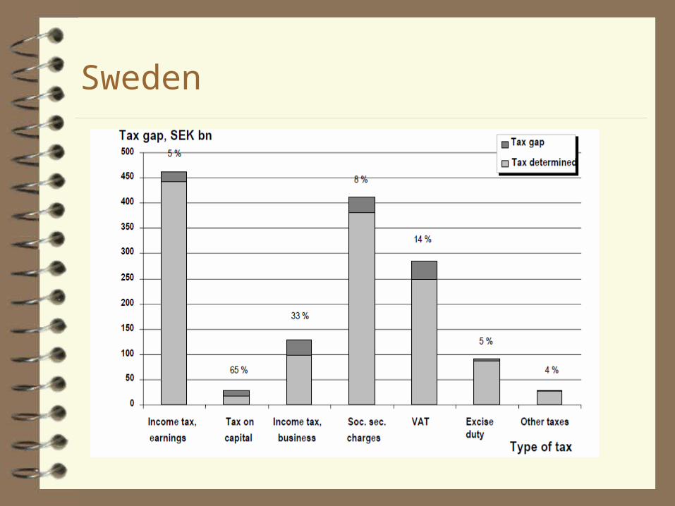
Sweden

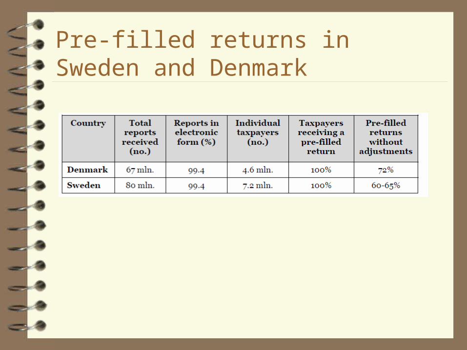
Pre-filled returns in Sweden and Denmark

Uses and misuses of tax gap

Uses– Reasonably good indicator of the order of

magnitude of tax non-compliance– Helpful for identifying key sources of non-

compliance– Underlying data can be useful for risk

assessment Misuses

– Short-term trend analysis– Performance evaluation

Digression on “closing the tax gap”

Public disclosure of tax gap estimates inevitably leads to demands to “close the gap”– Even under an optimal tax administration, it is

important to recognise that some gap will exist– Nor is it optimal to audit until MR=MC

Heisenberg uncertainty principal– Attempts to measure the tax gap impact its size– Attempts to reduce the tax gap impact the tax

base

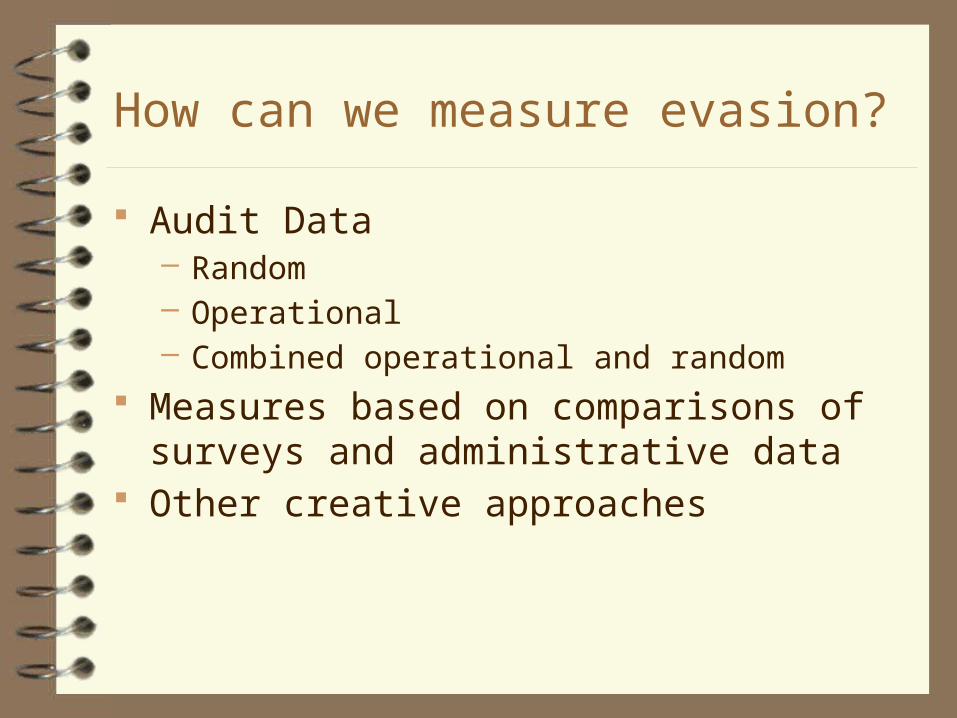
How can we measure evasion?

Audit Data– Random– Operational– Combined operational and random

Measures based on comparisons of surveys and administrative data

Other creative approaches

Designing random audit studies

Scope Scale Sampling strategy Data collection

Scope

May be interested in a particular tax or tax issue– Individual income tax, Corporate income tax, VAT– Specific credits, deductions, or income sources

May be interested in a particular taxpayer segment– Self-employed taxpayers, employers, high wealth

individuals – For instance, one may want to investigate compliance

by small businesses with all taxes (income tax, VAT/sales tax, employment taxes, etc.)

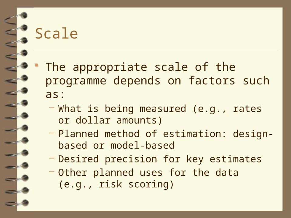
Scale

The appropriate scale of the programme depends on factors such as:– What is being measured (e.g., rates or dollar amounts)– Planned method of estimation: design-based or model-

based– Desired precision for key estimates– Other planned uses for the data (e.g., risk scoring)

Evolution of IRS random audit programs: Taxpayer Compliance Measurement Program (TCMP)

Line-by-line audits of a stratified random sample of about 50,000 individual income tax returns

Conducted approximately every 3 years from TY 1963 until TY 1988– Also occasional studies of other taxes (employment,

small corporations, partnerships, individual non-filers) Primary uses were:

– Development of audit selection criteria– Measurement of tax gap– Research

Long dry spell

13 years later … TY 2001 National Research Program (NRP)

– Stratified random sample of 45,000 individual returns for TY 2001– Advertised as “kinder and gentler” than TCMP

• About 10% of returns accepted without examination or with only a correspondence examination

• Not all line items examined – Some routinely examined – e.g., self-employment returns– Some examined only at discretion of “classifier” or

examiner– Case building materials provided in advance– For TY 2001, had a small “calibration sample” of returns audited

in a manner similar to old TCMP program • Useful for evaluating non-compliance on line items that were

not routinely examined

NRP redesign

Smaller annual studies of individual income tax– Most recently for tax years 2006, 2007, 2008– About 14,000 returns per year

No longer a calibration sample Some recent studies of other taxes

– S-corporations (tax years 2003 and 2004, 5,000 returns)– Employment tax (2008-2010, 6,000 returns)

Design challenges

Mandatory vs. discretionary examination of line items

Intensity of probes for unreported income sources Examination of related entities Adjustments following disputes and appeals If detection controlled estimation is to be

employed, ensuring sufficient examiners who have each done a reasonable number of audits of the return items of interest

Some best practices for random audit studies Non-sampling errors can plague a random audit study. The

following practices help to prevent such errors:– Appropriate support and training of examiners and other staff –

buy-in by examiners is crucial– Provide examiners with relevant case-building information– Design procedures to distinguish reports on the wrong line item

from reports of an incorrect amount– Have good procedures for recording, validating, and correcting

data– Record details on which specific line items or issues have been

examined and which have not– Provide adequate supervision

It is also useful to consider what auxiliary information to collect to aid research

Random sampling: design-based estimation Design-based estimation is very common in

survey work. Under this approach:– The variables of interest in the population are treated as

fixed but unknown numbers– Estimates are computed based on a randomly drawn

sample from this population (typically, these estimates are the sample analogues of the population characteristics of interest)

– The properties of the estimates (such as their means and variances) are derived using information only about the selection probabilities for the observations in the sample (i.e., the approach is non-parametric)

Estimating the rate of non-compliance

Canada Processing Review Programme– Approach is to contact a random sample of individual

taxpayers who have claimed certain credits or deductions to request receipts to verify their claims

– The results are used to measure the rates of non-compliance on these items and to develop targeting criteria for future verification work

Canada Core Audit Programme– Approach is to randomly audit various SME segments

for selected tax issues to estimate rates of material non-compliance and assess risks

Simple random sampling (SRS)

One starts with a sample frame– For this example, the frame is all tax returns in a given

year that claimed at least one specified credit or deduction

Under SRS, one randomly chooses returns from the sample frame in such a way that every possible sample of size n that can be drawn from the N returns in the population has an equal chance of selection

Point and interval estimation

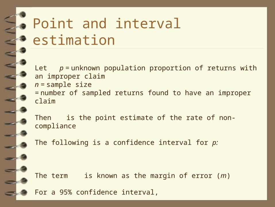
Let p = unknown population proportion of returns with an improper claimn = sample size= number of sampled returns found to have an improper claim

Then is the point estimate of the rate of non-compliance

The following is a confidence interval for p:

The term is known as the margin of error (m)

For a 95% confidence interval,

How large should the sample be?

Suppose we want to draw a random sample to estimate the rate of non-compliance with a margin of error m=.03 (for a 95% level of confidence). Since

we can calculate n as:

Of course, we don’t know p. The worst case scenario for precision is p=1/2, in which case: 

Some notes

If the population size N is relatively small, a somewhat smaller sample will be required. (We are ignoring the FPC factor

point estimate) If we are confident that the true rate p is far from

½, we can use a smaller sample

Estimating the magnitude of non-compliance Example: Kleven et al. (2011)

– As part of this study, a random sample of Danish taxpayers were selected for rather comprehensive audits of their personal tax returns

– The study was used for various purposes, including developing an estimate of overall tax underreporting

Summation notation

Population

Observation X 1 2 2 8 3 5 4 6 5 1

Total 22

N is population size (5 in this example)

𝑋𝑖𝑁

𝑖=1 = 𝑋1 + 𝑋2 + 𝑋3 …+ 𝑋𝑁

𝑋𝑖5

𝑖=1 = 2+ 8+ 5+ 6+ 1 = 22

Point estimationrepresent the overall magnitudes of tax underreporting on the N returns in the population

represent the overall magnitudes of tax underreporting on the n returns in a SRS from the population

represents the mean level of tax underreporting in the population

represents the aggregate level of tax underreporting in the population

Our respective point estimates of the mean and aggregate levels of tax underreporting in the population are:

Interval estimation

The population standard deviation of tax underreporting is defined as:

The interval estimates for the mean and aggregate levels of tax underreporting are, respectively:

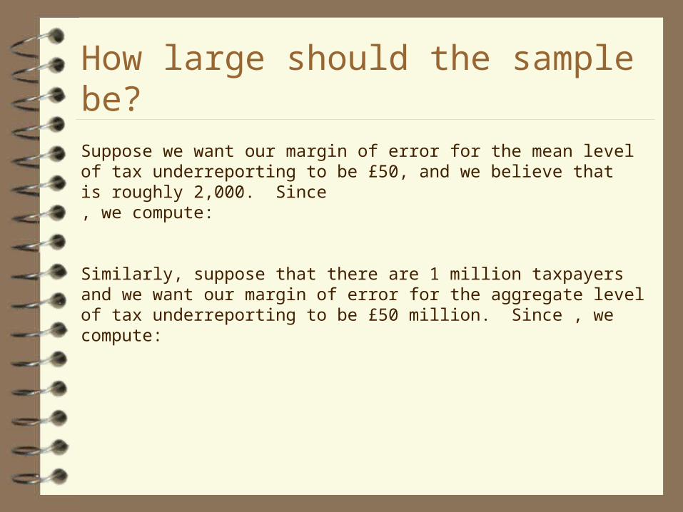
How large should the sample be?

Suppose we want our margin of error for the mean level of tax underreporting to be £50, and we believe that is roughly 2,000. Since, we compute:

 Similarly, suppose that there are 1 million taxpayers and we want our margin of error for the aggregate level of tax underreporting to be £50 million. Since , we compute:

So far, we have considered SRS. However, often it is preferable to use a stratified random sample.

One should do so if:– Reasonably precise estimates are desired for certain

subgroups of the population; or – The mean value of the variable of interest is likely to

differ substantially across different subgroups For instance, separate sampling strata were

defined for employment status (self-employed or not self-employed), return complexity, and region in the Denmark study

Stratified random sampling

Summation notation, continued

Population

Stratum Observation X 1 1 2 1 2 8 1 3 5

Subtotal 1 15 2 1 6 2 2 1

Subtotal 2 7 Total 22

Size of stratum 1: 𝑁1 = 3

Size of stratum 1: 𝑁2 = 2

Total for Stratum h: σ 𝑋ℎ𝑗𝑁𝐻𝑗=1 = 𝑋ℎ1 + 𝑋ℎ2 + ⋯+ 𝑋ℎ𝑁ℎ

If h = 1, σ 𝑋1𝑗𝑁1𝑗=1 = 𝑋11 + 𝑋12 + 𝑋13 = 2+ 8+ 5 = 15

If h = 2, σ 𝑋2𝑗𝑁2𝑗=1 = 𝑋21 + 𝑋22 = 6+ 1 = 7

Overall total:

𝑋ℎ𝑗 =𝑁ℎ𝑗=1

𝐻ℎ=1 𝑋11 + 𝑋12 + ⋯+ 𝑋1𝑁1 + 𝑋21 + ⋯+ 𝑋𝐻𝑁𝐻

𝑋ℎ𝑗 =𝑁ℎ𝑗=1

2ℎ=1 𝑋11 + 𝑋12 + 𝑋13 + 𝑋21 + 𝑋22 = 2+ 8+ 5+ 6+ 1 = 22

= 𝑋1𝑗𝑁1𝑗=1 + 𝑋2𝑗

𝑁2𝑗=1 = ሺ𝑋11 + 𝑋12 + 𝑋13ሻ+ሺ𝑋21 + 𝑋22ሻ= (15) + (7) = 22

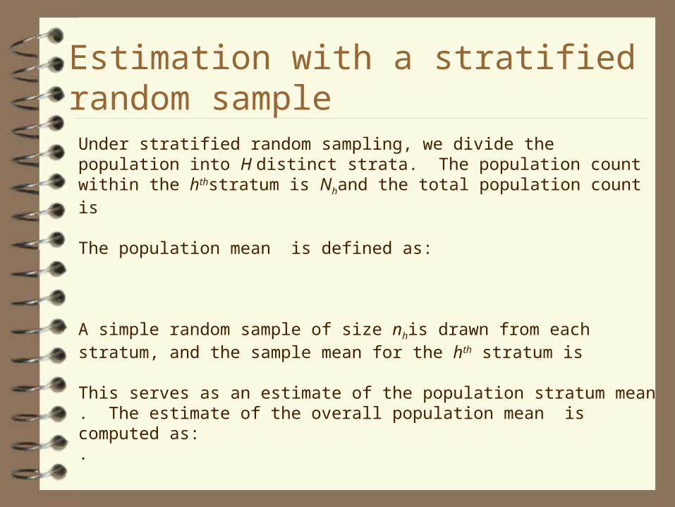
Estimation with a stratified random sample

Under stratified random sampling, we divide the population into H distinct strata. The population count within the hthstratum is Nhand the total population count is  The population mean is defined as:

 A simple random sample of size nhis drawn from each stratum, and the sample mean for the hth stratum is

This serves as an estimate of the population stratum mean . The estimate of the overall population mean is computed as:.

Sample weights

To simplify computation of sample statistics, one often constructs sample weights, which are defined as the inverse of the sampling rate within a stratum: for all taxpayers i in stratum h

So, for instance, the estimate of the population mean is computed as a weighted average over the entire sample:

Stratified sampling strategies

Proportional allocation: sample each stratum in proportion to its size in the population:

Optimal allocation: choose stratum sample sizes to maximise precision for a given overall sample size n– Suppose the cost of examining a return in stratum h is

ch

– Then the optimal allocation sets

Estimating rates vs. magnitudes

Estimation of rates of non-compliance tends to require a modest sized random sample (1,000 observations or less) for reasonable precision

The distribution of the magnitude of tax non-compliance tends to be highly skewed, resulting in a large population standard deviation – As a consequence, rather large samples are typically

required for adequate precision in estimating magnitudes

Model-based approaches with random audit data Under a model-based approach, one specifies a

relationship between the variable of interest (non-compliance) and its potential determinants

The model generally imposes functional form and distributional assumptions (parametric approach)

The quality of the estimates depends not only on the sample design but also the validity of the modelling assumptions

Why use a model-based approach?

To control for measurement errors, such as: – The failure to fully detect non-compliance– Conflation of deliberate and unintentional errors

To improve one’s understanding of what drives compliance behaviour and to predict future behaviour

Potentially, to improve the precision of tax gap estimates (if the underlying modelling assumptions are reasonably valid)

Old IRS Approach

Long ago, a study of randomly audited returns from TY 1976 found, with the aid of third party returns not available to the original examiners, that for every dollar of underreporting discovered for certain income items, another $2.28 went undiscovered

Based on this study, the IRS routinely applied a “multiplier” of 3.28 to detected unreported sources not subject to third-party reporting when estimating the tax gap

What we see

Random audit studies such as the TCMP and NRP tell us about audit assessments on different sources of income and offsets

So, they give us an idea of how much additional tax might be assessed if everyone received a fairly intensive audit

They also indicate what sorts of income and deduction items are commonly associated with compliance problems

What we don’t see

The objective of tax evasion is to conceal one’s actual tax liability…

Not infrequently, this is done so well that examiners are unable to uncover all of the cheating that is present on a return

So audit assessments allow us to observe most of the unintentional errors and much of the deliberate cheating that is fairly easy to identify

However, they show us only a portion of the deliberate cheating that is hard to uncover

How to measure what we can’t see

Intuitively, some examiners are better at uncovering noncompliance than others– Some might be globally superior on all return issues;

others may have a comparative advantage on particular issues

If we knew the relative abilities of different examiners on a given issue or line item, we could “scale up” what was detected by a given examiner to approximate what the best examiner would have found if (s)he had done the audit

Detection Controlled Estimation (DCE)

A statistical methodology to account for detection errors on examinations and inspections

Original methodology developed by Jonathan Feinstein – Rand (1991), J. of Law & Economics (1990)

Improved and extended approach for use with NRP data in collaboration with Jonathan

Visualizing the approach: Suppose audit results show this:

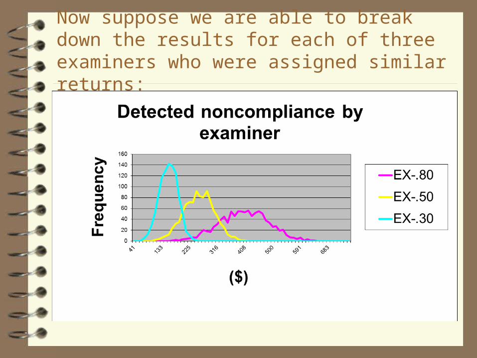
Now suppose we are able to break down the results for each of three examiners who were assigned similar returns:

Detected vs. actual non-compliance

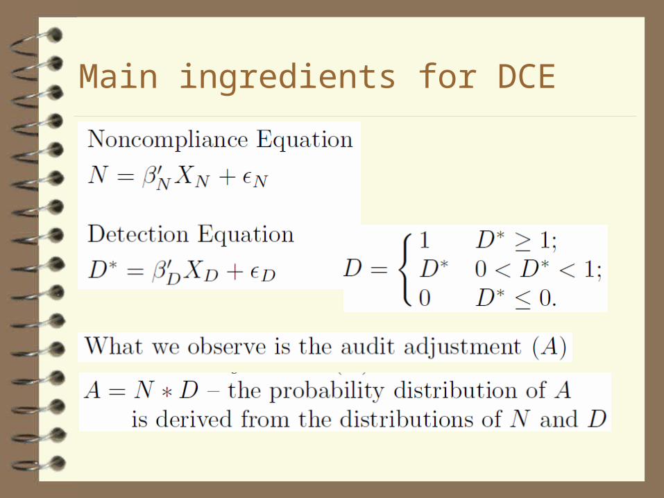
Main ingredients for DCE

Probit model with perfect detection (A=N)

DCE probit model

Regular tobit model with perfect detection (A=N)

p.d.f. of A

DCE tobit model: pdf of

When A = 0, just like DCE probit case: Pr(A=0) = When A>0, p.d.f. is sum of expressions for 2 separate kinds of detection outcomes:1. Perfect detection: 2. Partial detection: account for all D rates 0 to 1:

The 1/D term in the integral is the Jacobianof the transformation from N to A

DCE tobit likelihood function for independent normal disturbances

A=0:

A>0:

Extensions of approach Model the probability and magnitude of non-compliance

using separate equations Account for skewness in distribution of non-compliance Account for role of third-party information reports Employ separate models for each income source Account for cases where an income source was not

examined during the audit Separately model the case where an income source has not

been reported on the return Pool data from multiple tax years Incorporate results into a micro-simulation model

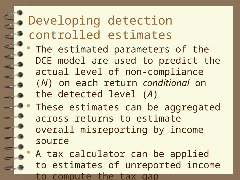
Developing detection controlled estimates The estimated parameters of the DCE model are

used to predict the actual level of non-compliance (N) on each return conditional on the detected level (A)

These estimates can be aggregated across returns to estimate overall misreporting by income source

A tax calculator can be applied to estimates of unreported income to compute the tax gap

One can also use the results to derive implicit DCE multipliers

Confidence intervals Our aggregate estimate of underreported income is

S= Approach 1: Delta method

– , where – G is estimated gradient vector – is estimated covariance matrix of

Approach 2: Simulation– Draw M random samples of parameter vector from a distribution

with mean and covariance – For each draw, compute an estimate of S – Sort the sample values of S and use the ndand 1-nd percentiles as the

upper and lower bounds

Implicit DCE multipliers for TY 2001

Estimates of net income misreporting

Notes on DCE methodology

Relies on variation across examiners in their performance at uncovering unreported income– The method essentially scales up performance of all

examiners to reflect what the best examiner would have found

– Sometimes there are not sufficient examiners who have each audited an income source on a reasonable number of returns. One can do some pooling in such cases

To help insure model identification, it is desirable not too have much overlap between the explanatory variable sets XN and XD

Attempting to distinguish deliberate from unintentional errors: a simple example

Extensions

Use separate equations to describe the probability and magnitude of non-compliance

Account for undetected non-compliance

Tax gap estimation with operational audit data Operational audits are generally undertaken on

returns where substantial non-compliance is deemed likely

This creates a classic sample selection problem– The audited returns are unlikely to be representative of

unaudited returns

Sample selection example

During WWII, engineers routinely examined damage to returning bombers

– They reasoned that those areas that were consistently shot up would benefit from more reinforcement

Their concern, of course, was improving the odds that an aircraft would return successfully; yet the sample consisted only of aircraft that did return

Abraham Wald insightfully turned the “common wisdom" on its head

How to control for sample selection bias

Statistical models of sample selection– In research for the IRS, I have used this approach to

estimate the estate tax gap and also to investigate underreporting of self-employment income

Statistical matching

Statistical models of sample selection

The selected sample may differ from the general population in terms of both observed and unobserved characteristics

Under this approach, one attempts to account for both the observed and unobserved differences

One does this by jointly modelling the determinants of the outcome variable of interest and the sample selection process

Heckman (1979) sample selection model

Correlated errors case

A two-part sample selection model of tax non-compliance

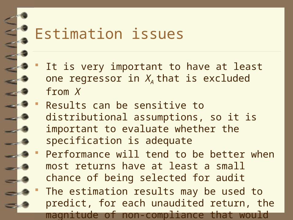
Estimation issues

It is very important to have at least one regressor in XA that is excluded from X

Results can be sensitive to distributional assumptions, so it is important to evaluate whether the specification is adequate

Performance will tend to be better when most returns have at least a small chance of being selected for audit

The estimation results may be used to predict, for each unaudited return, the magnitude of non-compliance that would have been discovered if the return had been audited

Statistical matching

Attempt to control for observed differences between operational audit sample and unaudited returns

No attempt to control for unobserved differences– Likely to work best with a detailed data base that

includes the most important factors impacting whether a return is selected for an operational audit

Often used to evaluate treatment effects– But it can be used to impute, say, non-compliance from

operationally audited returns to unaudited returns

Key assumptions

Let A = audit indicator (A=1 if audited, 0 otherwise)N = Non-compliance if not auditedX = set of explanatory variables1. A|X (conditional independence or unconfoundedness 2. 0 < (common support)3. X is exogenous (not influenced by A)

Relationship between statistical matching and random assignment Random assignment

– Distribution of both measured and unmeasured variables balanced across groups

– Common support condition always holds Matching

– Only distribution of measured variables balanced across groups

– Common support condition may fail for some values of X

Relationship between statistical matching and regression analysis Matching is non-parametric

– No need to assume functional forms (linearity, additive errors, normality, etc.)

Common support requirement avoids the extrapolation problem in regression– Identifying effects by projecting into regions where no

data points exist

Matching approaches

Exact match on X– Useful if small number of qualitative variables in X

Inexact match on X– A distance metric is used to find one or more audited

returns that have similar X values to each audited return Propensity score matching

– Idea is to reduce dimensionality of the problem by matching on a single index:

– Rosenbaum and Rubin (1963) showed that if then A|

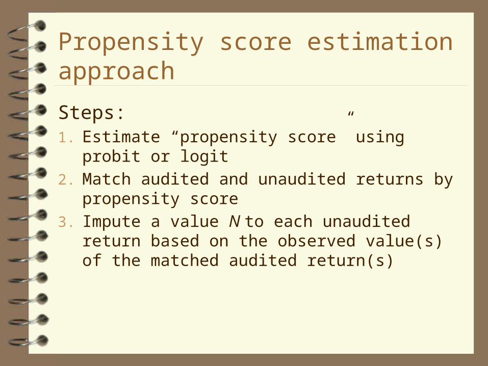
Propensity score estimation approach

Steps:1. Estimate “propensity score” using probit or logit2. Match audited and unaudited returns by propensity score3. Impute a value N to each unaudited return based on the

observed value(s) of the matched audited return(s)

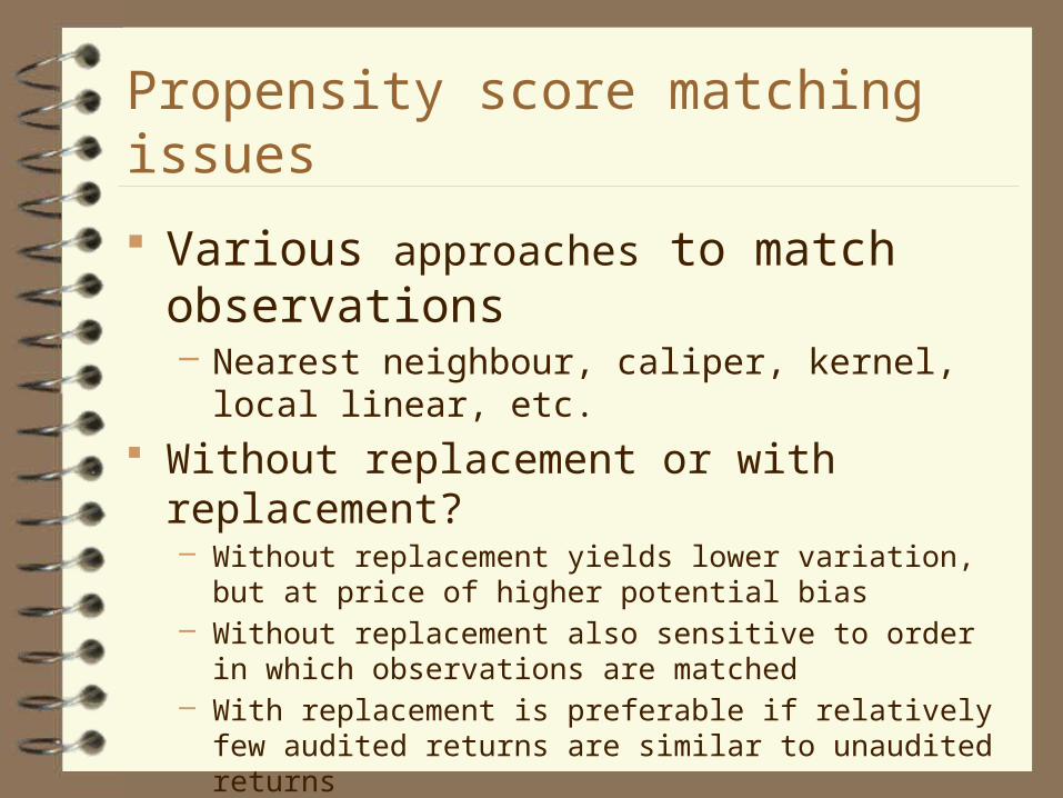
Propensity score matching issues

Various approaches to match observations– Nearest neighbour, caliper, kernel, local linear, etc.

Without replacement or with replacement?– Without replacement yields lower variation, but at price of higher

potential bias– Without replacement also sensitive to order in which observations

are matched– With replacement is preferable if relatively few audited returns are

similar to unaudited returns Balancing conditions: want

– Good to break into 5 or so strata and verify mean values of X within each stratum are similar for audited and unaudited returns

Choice-based sample

If the sampling probability depends on whether return was audited (e.g., oversampling of audited returns), one can– Perform an unweighted logit analysis to estimate

parameter vector – Perform an unweighted logit analysis and match

observations using the estimated log odds ratio:

Alternatively, one can perform weighted logit (or probit) and use usual propensity score

Creative and interesting power law application Zipf’s Law postulates that the size (S) or frequency of

an observation is inversely proportional to its rank (R):

– It has many applications (size of cities, frequency of words in a book, income rankings, corporation size, number of visits to websites, etc.)

– It is “power law” relationship (also known as Pareto) and often fits the upper tail of a distribution well

Bloomquist, Hamilton, and Pope (2013) fit a size-rank regression to operational audit results to estimate overall non-compliance among very large corporations (over US$250 million)

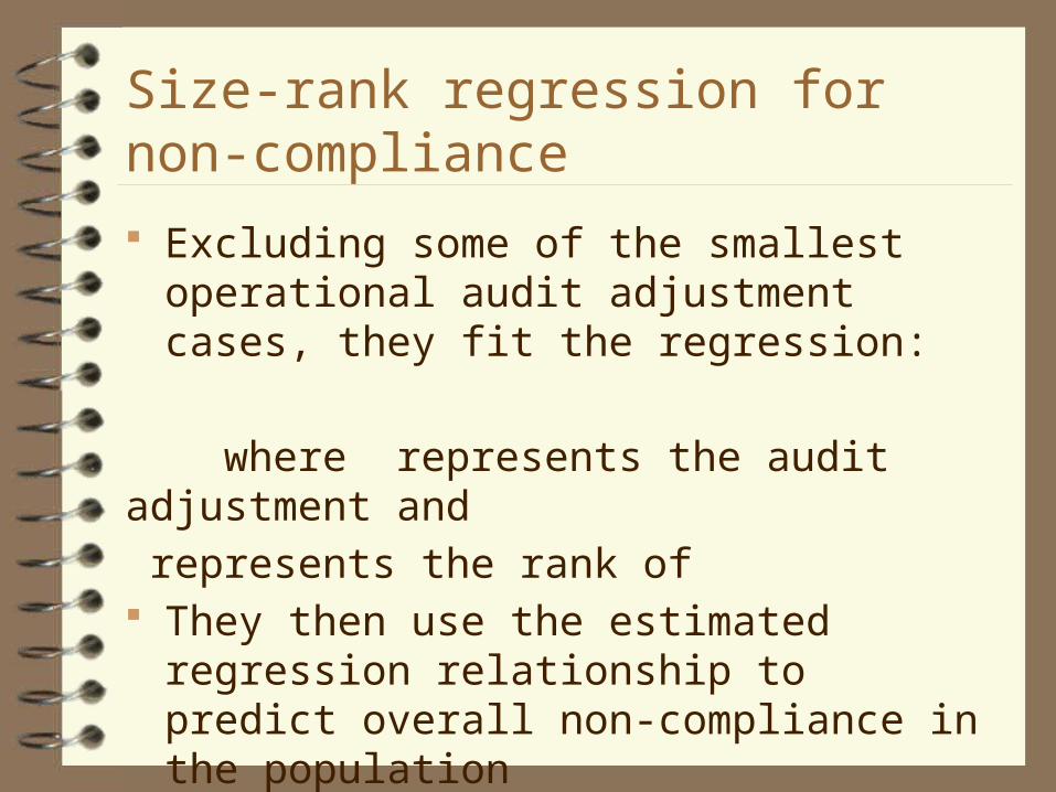
Size-rank regression for non-compliance

Excluding some of the smallest operational audit adjustment cases, they fit the regression:

where represents the audit adjustment and represents the rank of They then use the estimated regression

relationship to predict overall non-compliance in the population

Possible issues for further exploration

Zipf’s Law seems unlikely to hold towards the bottom of the size-rank distribution in the population where non-compliance is zero or negative (i.e., overstatements of income)

The ranks of observations within the estimation sample will tend to be more concentrated than the ranks of the same observations in the population– It is not clear how much this impacts predictions

The results may be somewhat sensitive to the chosen adjustment amount threshold for inclusion in the size-rank regression

Observations

Approach is relatively simple to apply and it accounts the important fact that a relatively small number of extreme cases account for the bulk of non-compliance

Approach yields an aggregate estimate– It does not facilitate an analysis of the determinants of

underreporting– In principle, though, one could extend the approach to

derive separate aggregate estimates for different income sources or for different categories of corporations (industry, public/private, national/international, etc.)

Combining operational and random audit dataIdeally, “round out” operational audit with some random audits of untargeted returns (and, ideally, non-targeted issues)

Selected for Operational Audit

Not selected for Operational Audit

Issues with operational-random sample Based on a study I performed for the IRS:

– Design-based estimation of such a sample is not very promising – one needs a rather large random component to obtain reasonable precision

– Model-based estimation that incorporates sample weights is known to provide a degree of protection from misspecification. However, weighted estimation adversely impacts precision, especially when weights vary substantially in the sample.

– Although unweighted model-based estimation can lead to incorrect inferences if the modelling assumptions are invalid, a well-specified model can achieve superior precision in a combined sample with a large number of targeted audits and relatively few untargeted ones.

It would seem ideal to integrate random sampling into an operational audit selection program

Value of audit data for targeting non-compliance Random audit findings can be used to devise audit

selection strategies– NRP and DIF-selection in U.S.

Operational audit findings alone are not adequate for developing audit selection criteria– Tunnel vision

A combined operational-random sample may be a viable alternative

Survey discrepancies Surveys that directly ask about tax evasion are not

especially useful– Although there has been some success with asking

about informal sector employment (e.g., Lemieux et al., 1994)

Comparison of survey reports on income or expenditure with tax data more promising– Informal supplier evasion– “Nanny Tax” evasion– Non-filers

U.S. informal suppliers

The IRS defines informal suppliers as “individuals who provide products or services through informal arrangements which frequently involve cash-related transactions or ‘off the books’ accounting practice”

Owing in large part to the lack of a ‘paper trail’ tax non-compliance among informal suppliers can be especially difficult to detect

Past IRS methodology

In the past, the IRS commissioned a special survey of consumer purchases that attempted to assess informal earnings based on reported expenditures on informally supplied goods and services

It was not clear how successful this research was in distinguishing informally from formally supplied goods and services

A new approach

Jim Alm and I took a different approach. Rather than rely on a dubious distinction between formal and informal sales, we identified 12 industries where informal suppliers are prevalent (food vendors, direct sales, construction, landscaping, personal services, etc.)

We then compared reported self-employment earnings in these industries from a large national survey to tax return reports from these same industries

Our approach attempts to account for all earnings in these industries from self-employment, including that earned through moonlighting

Findings

Our results yield a higher level of non-compliance in these industries than NRP-auditors were able to uncover through intensive audits of tax returns

At the same time, our estimates are somewhat lower than the DCE-adjusted NRP estimates. – This makes sense, since some self-employed

individuals may not be fully forthcoming about their earnings, even on an anonymous national survey

Who’s minding the Nanny Tax?

In the U.S. households are responsible for paying various employment taxes when they pay more than a nominal amount for the services of a domestic employee (nannies, housekeepers, home health aides, cooks, butlers, chauffeurs, groundskeepers, etc.)

Household employers are required to file Schedule H with their income tax returns to report all such payments

Together, federal and state employment taxes amount to more than 20% of domestic employee compensation

Compliance study methodology

To examine compliance with Nanny Taxes, I used a large national survey to identify individuals who report that their longest job held during the year was from domestic employment in a household

Based on their reported earnings from this job, I estimated how many Nanny Tax returns should have been filed

The results indicate that only 1 in 4 domestic employers actually file and pay Nanny Taxes, and that in aggregate, only about half of the federal taxes due are actually paid

Validation of estimates

Concerns with the methodology include:– Moonlighters are excluded– Some domestic workers are likely to be reluctant to

report their earnings on the survey As a validation exercise, I used a national

consumer expenditure survey to investigate how much household reported spending on in-home child care and house cleaning– The results suggest non-compliance is even worse,

perhaps as high as 70% of taxes due

Individual income tax filing rate estimation IRS is interested in measuring the trend in the

voluntary filing rate (VFR), defined as the ratio of timely filed required returns to required returns

I worked with Alan Plumley and Mark Payne of the IRS to develop an improved filing rate measure

Measuring the numerator of the VFR

To measure the numerator of the VFR, a large representative sample of filed individual returns was analyzed to estimate the number of timely filed required returns– Some filed returns are not required– In the process of distinguishing required from non-

required returns, we discovered that IRS instructions on who must file are incomplete

– Our findings led to a change in IRS instructions to clarify that the gross income concept for filing purposes disregards all losses

Estimation of denominator of VFR

We relied on a large national survey to identify households that appeared to have a filing requirement

To address underreporting of certain income sources on the survey, we imputed additional self-employment earnings, pensions, and social security to various households– The imputations were based on an econometric

analysis of 3rd party reports (for pensions and social security) and tax returns (for self-employment earnings)

Findings

The bump in the filing rate in TY2007 coincides with the “Economic Stimulus Payment” (worth $300 per family member), suggesting that this one-time benefit encouraged many ghosts to file a return in that year.

Idea to evaluate the determinants of filing compliance – “calibrated probit”

Tax return data: =1 for all observations i = 1,…,Survey data: is unknown for all observations j = 1,…,n Survey weights: (Overall population of filers and non-filers)

Constrained estimation of parameters:Maximize s.t.

Other creative approaches for measuring non-compliance Searching for non-filers in Jamaica Searching for traces of evasion

– In consumption behaviour– In litter

Searching for non-filers in Jamaica

Prior to the 1986 reform, Jamaica had high marginal tax rates, but many credits and loopholes

Wage earners were taxed via PAYE withholding, while self-employed were required to file a return

Alm, Bahl, and Murray (1991) methodology

The authors sampled 12,000 names from a master population list based on third-party sources of information (telephone directories, trade association lists, etc.) on workers in 9 industries (service stations, customs brokerages, auto repair, auto parts, hair care, real estate, contractors, transport, beverage and spirits outlets)

A similar approach was used to sample 600 professionals (accountants, architects, attorneys, doctors, etc.)

The sampled names were matched against Jamaica Income Tax Department records to check filing and withholding status

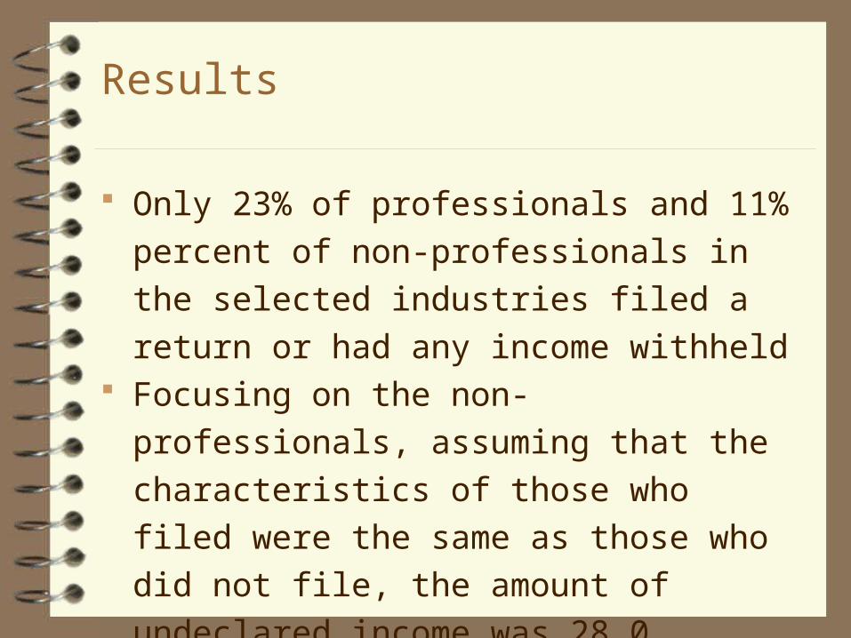
Results

Only 23% of professionals and 11% percent of non-professionals in the selected industries filed a return or had any income withheld

Focusing on the non-professionals, assuming that the characteristics of those who filed were the same as those who did not file, the amount of undeclared income was 28.0 percent of reported income, costing the government 38.8 percent of actual income taxes collected

Searching for traces of evasion in consumption behaviour Since consumption behaviour tends to be closely

linked to income, the idea is to infer underreporting of income in cases where consumption appears to be excessive in relation to income– Pissarides and Weber (1989)– Feldman and Slemrod (2007)– Fu (2008)

Pissarides and Weber (1989)

Assume food expenditures and wages are reported accurately on national survey, but not income from self-employmentEstimate a consumption function:

where lnY = reported incomeSE = dummy variable for self-employment Z = demographic controls

Data source: 1982 Family Expenditure Survey – diary records for food consumption usedActual SE income could then estimated as exp( (the actual analysis they use is a bit more complex)

Results

The estimated coefficient of the SE dummy () is about 0.10, while the estimated mpc () is roughly 0.25, implying that actual self-employment income is about exp(.10/.25)=1.5 times as large as the reported amount (33% underreporting)

Possible issues – The self-employed may be more prone to eating out,

buying meals for their clients, etc.– What the self-employed report as earnings on a survey

may be different than what they report on their tax returns

Feldman and Slemrod (2007) Apply a similar approach to measure tax evasion in U.S.

by self-employed, but with charitable donations used in place of food expenditures– Since charitable contributions are only reported by itemizers,

authors have to control for price of giving in their analysis The data source is a large public use sample of federal

individual income tax return data (both cross-sectional and longitudinal)

The key assumption is that self-employment status does not impact the true propensity to make donations

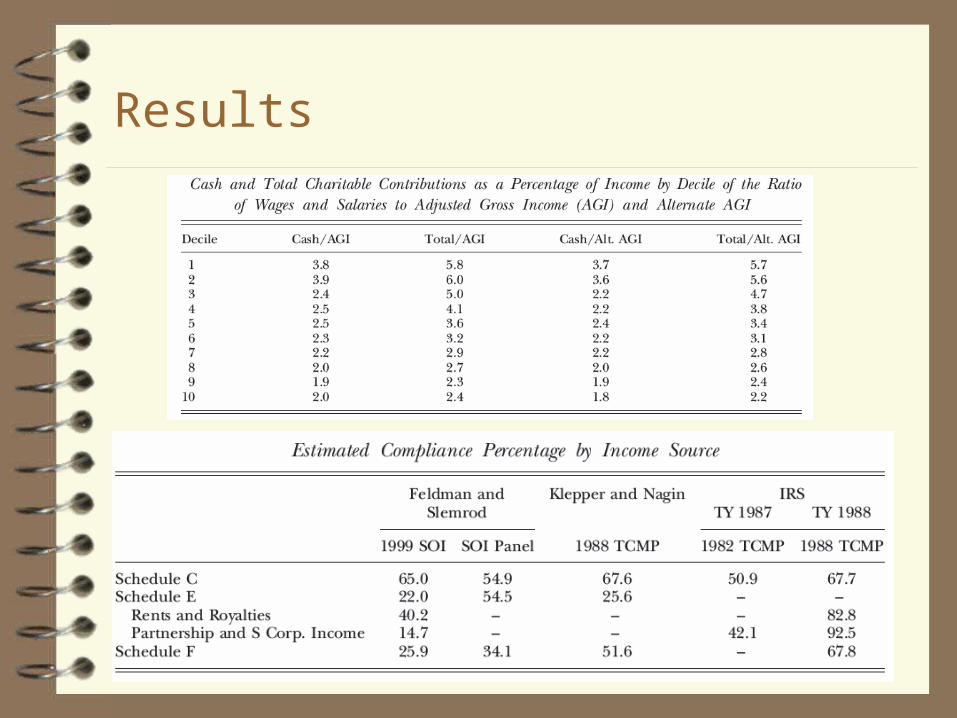
Results

Fu (2008) Instead of “inverting” a consumption function to predict

true income, Fu searches for discrepancies between income reported on Canadian individual tax returns and an imputed measure of overall consumption and savings

Data sources– Regression on Survey of Household Spending (SHS)

used to develop prediction formulae for consumption and savings

– Prediction formula applied to Survey of Financial Security (SFS) to impute consumption and savings• SFS already has detailed information on income reported on

tax returns

Consumption regression

Total household consumption regression:

where Z = common consumption sources on the2 surveysX = demographic factors, reported income, mortgage to income ratio, and rent to income ratioSeparate approaches attempted with and without including durable consumption

Findings

Even just imputing $8/day for food, clothing, and transportation on top of ongoing expenses in SFS implies 8% of wage earners and 20% of self-employed have an income statement discrepancy

Using SHS to impute consumption yields an estimated incidence of underreporting of 25% for non self-employed and 60% for self-employed (higher if durable consumption is included)

Issues

Income measure in two data sources may differ; not clear how this impacts imputations, which include income as an explanatory variable

Method assumes that consumption and savings self-reports are accurate

Imputations at the individual level likely to be rather noisy– Some sensitivity analysis was done

Searching for traces of non-compliance in litter In 2007, state and local cigarette taxes in Chicago

in were $2.68 per pack higher than in neighboring counties and over $3.10 higher than in the bordering state of Indiana

Cigarette packages are required to have tax stamps affixed to them to demonstrate that required taxes have been paid

Smokers in Chicago have incentives to purchase cigarettes from lower tax jurisdictions directly or from smugglers and/or Native American reservations

Merriman (2010) methodology

Students worked in teams to find and collect littered cigarette packs in randomly selected representative tracts in Chicago and some neighbouring locations

The location of each pack was logged along with information about the presence or absence of tax stamps from different jurisdictions

Findings

75% of sampled cigarette packs from the Chicago area did not have a Chicago tax stamp (indicating the packs were purchased from other lower tax counties or states, or from contraband suppliers)

The share of packs with a Chicago tax stamp was lowest in Chicago neighbourhoods close to the lower cigarette tax state (Indiana)

More generally, regression analysis indicated that the share of Chicago tax stamps in a location was negatively associated with the distance to a lower tax jurisdiction and with the level of tax savings

Selected empirical approaches

Econometric models using random audit data

Aggregate panel data on tax reporting by state/jurisdiction, supplemented by socio-economic variables

Lab Experiments Field Experiments Agent-Based Models

Econometric models using random audit data

NRP Study Findings– Tax rates, income: hard to identify in a cross-section; Feinstein

(1991) pools 2 years and finds tax rate positively related to non-compliance and income not significant

– Tax Preparers: Klepper et al. (1991) find preparers enforce unambiguous tax rules and exploit ambiguous ones; Erard (1993) finds preparers (especially CPAs and attorneys) are associated with greater non-compliance

– Prior Audits: Erard (1992) finds weak evidence that audits positively impact future reporting behaviour

– Demographics: elderly less likely to cheat; married more likely

Aggregate panel data findings

Dubin et al. (1990), Plumley (1996), Dubin (2007) find very large general deterrent effect of audit rates

Plumley, Erard, and Snaidauf (2011) find predictions sensitive to specification decisions:– Trend vs. year dummies– Time period– Dynamics

Lab experiments

Can test theoretical predictions/hypotheses in a controlled setting– Isolate a particular factor to change, holding all other

factors constant However, the test is somewhat weak in that setting

is artificial (external validity is unclear):– Salience: hard to capture moral and social influences,

real world costs and benefits – I might cheat on taxes in a lab setting (just a game from my perspective), but much more inclined to be honest in actual practice

Lab experiment findings

Many studies by Alm et al. on myriad of factors Impact of some key factors on compliance:

– Tax rates -– Audit rates + (modest)– Fine rates + (small)– Positive inducements + – Vote over use of tax revenue (public good) +

Replication of experiments across different countries indicates that cultural factors/experience impact behaviour

Field experiment: Slemrod et al. (2001)

Randomised field experiment in Minnesota – treatment sample told in advance their returns would be “closely examined”; DIF-in-DIF analysis of reported taxes before/after treatment– Low and middle income/high opportunity groups big

increase reported taxes– High income/high opportunity group results “perverse”

DIF-in-DIF approach

Timet = -1 t = 1post-treatment

= Impactof the program

pre-treatment

Control

t = 0

Field experiment Kleven et al. (2011)

Denmark: large scale (40,000 taxpayers) randomised field experiment; DIF-in-DIF on reported adjustments to income on pre-populated returns– Case 1: Threat of audit letters sent to a treatment group

• Significant improvement in reporting of self-reported income (income not subject to 3rd party reports)

– Case 2: Randomly audited and non-audited taxpayers in 2007 investigated for change in reported income in subsequent year• Significant improvement in compliance associated with prior

audit in 2007

Agent-Based Models (ABMs)

Bloomquist (2012) simulates tax compliance within a large community of taxpayers, employers, and tax preparers

Assumes certain behavioral rules for the various “agents” Allows communication among social networks One simulation experiment involves testing impact of

alternative audit selection strategies on taxpayer reporting. The results illustrate that targeted audits tend to be more effective at improving compliance

Strengths: allows analysis of complex social interactions and behaviors that are not analytically tractable

Weakness: Little existing evidence to guide behavioral rules practiced by different agents