Measuring Round Trip Times to Determine the Distance Between WLAN Nodes

Measuring Round Trip Times to Determine

the Distance between WLAN Nodes �

Andre Gunther and Christian Hoene

Telecommunication Networks Group (TKN), TU-Berlin, [email protected]|[email protected]

Abstract. This publication explores the degree of accuracy to whichthe propagation delay of WLAN packets can be measured using today’scommercial, inexpensive equipment. The aim is to determine the distancebetween two wireless nodes for location sensing applications. We con-ducted experiments in which we measured the time difference betweensending a data packet and receiving the corresponding immediate ac-knowledgement. We found the propagation delays correlate closely withdistance, having only a measurement error of a few meters. Furthermore,they are more precise than received signal strength indications.To overcome the low time resolution of the given hardware timers, variousstatistical methods are applied, developed and analyzed. For example,we take advantage of drifting clocks to determine propagation delaysthat are forty times smaller than the clocks’ quantization resolution.Our approach also determines the frequency offset between remote andlocal crystal clocks.

1 Introduction

Knowing the position of wireless nodes is required for location-aware servicesand applications. The position can be calculated using the distance betweenwireless nodes. Furthermore distance helps when deciding the time of handoversor finding the optimal routing path throughout an ad-hoc network.

In this paper we focus on locating techniques which use the intrinsic fea-tures of WIFI based wireless access. Usually, received signal strength indicationsare applied to identify the location of wireless nodes. We show that precise dis-tance measurement based on round trip time measurements of WLAN packetsis possible even with low-cost, commercial WLAN hardware. We developed thealgorithms to determine the air propagation time indirectly and to improve theaccuracy and resolution of the time measurements. We validated our approachwith two independent experimental measurement campaigns and with an ana-lytical explanation.

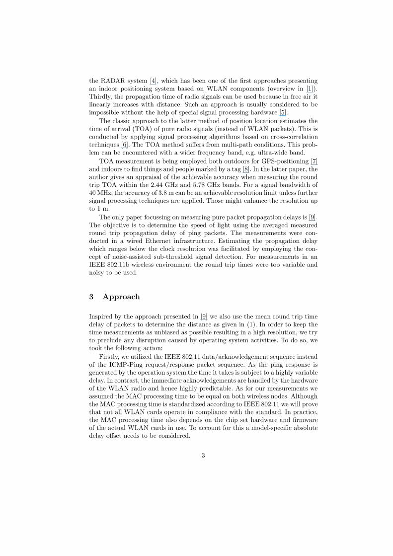
We utilize the following intrinsic feature of IEEE 802.11: Each unicast datapacket is immediately acknowledged by its receiver (Fig. 1). We took the time

� This work has been supported by the Deutsche Forschungsgemeinschaft (DFG). Thispublication is a condensed and enhanced version of [1]

between starting the transmission of a data packet and receiving the correspond-ing immediate acknowledgement. We will refer to this as remote delay (dremote).We also measured the duration of receiving one data packet and sending outthe immediate acknowledgement. We will call this duration local delay (dlocal).The overall propagation time is then estimated by subtracting the local fromthe remote delay.

c =2 · distance

dremote − dlocalwhere c ≈ 3 · 108 m

s being the speed of light. (1)

Fig. 1. Distance measurement: Transmission ofan ICMP ping sequence.

In order to overcome theproblem of interrupt laten-cies and hence inaccuracieswhen measuring the durationof packet transmission in theoperating system, we mea-sured the time on the hard-ware layer - the WLAN card.Most WLAN solutions allowto record time stamps at aresolution of 1 µs. However,a packet travels a distance of300 m in 1 µs, which usuallyexceeds the range of WLANtransmission. We increase theresolution by using multipledelay observations and apply-ing statistical methods to en-hance the accuracy.

This paper is structured as follows: In Sect. 2 we refer to the state of theart. Then we explain our approaches to enhance the measurement resolution. InSect. 4 we describe our experimental measurement campaigns. Finally, we brieflysummarize the results and contributions of this paper.

2 Related Work

A couple of approaches to in- and outdoor location sensing techniques have beenpresented in [2]. An essential part of location sensing algorithms is a method todetermine the distance between two wireless nodes. In general, three methodshave been considered. Firstly, in case of densely populated networks such assensor networks [3] the information about which nodes are within transmissionrange is used. Secondly, the received signal strength indication (RSSI) of datapackets transmitted is considered. It decreases sharply in a non-linear fashionwith distance, so that environment specific signal strength maps relating RSSIvalues to positions have to be created first. An example for RSSI application is

2

the RADAR system [4], which has been one of the first approaches presentingan indoor positioning system based on WLAN components (overview in [1]).Thirdly, the propagation time of radio signals can be used because in free air itlinearly increases with distance. Such an approach is usually considered to beimpossible without the help of special signal processing hardware [5].

The classic approach to the latter method of position location estimates thetime of arrival (TOA) of pure radio signals (instead of WLAN packets). This isconducted by applying signal processing algorithms based on cross-correlationtechniques [6]. The TOA method suffers from multi-path conditions. This prob-lem can be encountered with a wider frequency band, e.g. ultra-wide band.

TOA measurement is being employed both outdoors for GPS-positioning [7]and indoors to find things and people marked by a tag [8]. In the latter paper, theauthor gives an appraisal of the achievable accuracy when measuring the roundtrip TOA within the 2.44 GHz and 5.78 GHz bands. For a signal bandwidth of40 MHz, the accuracy of 3.8 m can be an achievable resolution limit unless furthersignal processing techniques are applied. Those might enhance the resolution upto 1 m.

The only paper focussing on measuring pure packet propagation delays is [9].The objective is to determine the speed of light using the averaged measuredround trip propagation delay of ping packets. The measurements were con-ducted in a wired Ethernet infrastructure. Estimating the propagation delaywhich ranges below the clock resolution was facilitated by employing the con-cept of noise-assisted sub-threshold signal detection. For measurements in anIEEE 802.11b wireless environment the round trip times were too variable andnoisy to be used.

3 Approach

Inspired by the approach presented in [9] we also use the mean round trip timedelay of packets to determine the distance as given in (1). In order to keep thetime measurements as unbiased as possible resulting in a high resolution, we tryto preclude any disruption caused by operating system activities. To do so, wetook the following action:

Firstly, we utilized the IEEE 802.11 data/acknowledgement sequence insteadof the ICMP-Ping request/response packet sequence. As the ping response isgenerated by the operation system the time it takes is subject to a highly variabledelay. In contrast, the immediate acknowledgements are handled by the hardwareof the WLAN radio and hence highly predictable. As for our measurements weassumed the MAC processing time to be equal on both wireless nodes. Althoughthe MAC processing time is standardized according to IEEE 802.11 we will provethat not all WLAN cards operate in compliance with the standard. In practice,the MAC processing time also depends on the chip set hardware and firmwareof the actual WLAN cards in use. To account for this a model-specific absolutedelay offset needs to be considered.

3

Secondly, we do not measure the time stamps for packet arrival and trans-mission on the operating system layer, but on the WLAN card hardware layer.This features measuring conditions that are independent of variable interruptlatencies. In [10] we showed that measuring the time of a packet’s arrival inthe operating system’s kernel (e.g. during an interrupt) entails quite impreciseresults due to falsification by the variable interrupt latency.

The resolution of these hardware time stamps, which are implemented inmost current WLAN products, is 1 µs corresponding to 300 m. In terms of theachievable accuracy this discrete time resolution is not precise enough yet. Theresolution increases when averaging numerous observations. In the following weconsider three phenomena that help to achieve a higher resolution.

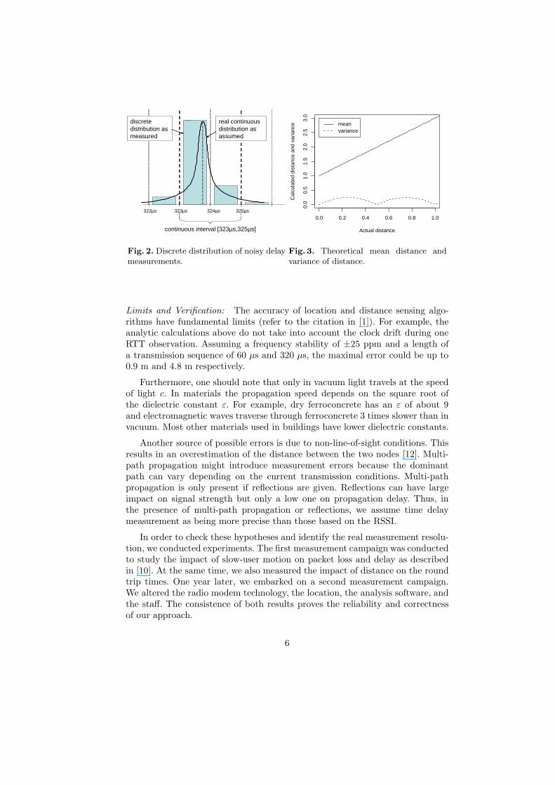
Gaussian noise: The presence of measurement noise is assumed. Noise can becaused by thermal noise in the received radio signal or by the presence of multi-path environment. Also, the crystal clocks of the WLAN equipment are subjectto a constant clock drift and variable clock noise. Thus, the delay values arenot limited to only one value. (In Fig. 2 not only 323 µs can be observed butalso other values). If one assumes a Gaussian noise distribution with a suitablestrength, we can simply take the sample mean to enhance the resolution.

Stochastic Resonance: Instead of the explanation above the authors of [9]suggested another statistic effect called stochastic resonance. The concept ofstochastic resonance was originally introduced as an explanation for the period-ically recurrent ice ages. In the last two decades, it has been applied to explainmany physical phenomena [11]. In the realm of signal detecting stochastic res-onance allows for detecting signals below the resolution of the measuring unitsbecause the signal becomes detectable with the help of noise. Noise adds to thesignal so that it eventually exceeds the threshold given by the resolution of thedetecting device. Thus, the system is able to change its states. The state dura-tions have random lengths, but the probability is high that one state remainsthe same in the next observation.

Beat Frequencies: In our experiments (Fig. 4.3 in [1]) it can be observed thatthe 323 and 324 values occur in blocks of regular patterns. But this effect cannotbe explained with the effect of stochastic resonance. Another effect can alsoentail resolution enhancement even if measurement noise is missing: ’Relativeclock drift’ – both WLAN cards are driven by built-in crystal oscillators thathave nearly the same frequency. Due to tolerances, there is a slight drift betweenboth clocks which causes varying rounding errors.

Let us consider the impact of a discrete time resolution on the measurementerror. Firstly, we construct a model of the experiment setups. Instead of usingpackets, we assume that a delta pulse is sent off from the local to the remote node.After the delta pulse’s arrival another delta pulse is sent back to the local noderepresenting an acknowledgement. The local node can only process the impulsesonly in discrete time steps tlocal ∈ N described with natural numbers. The sameis also valid for the remote node. It only reacts in discrete time steps, which are

4

tremote = δ + n where n ∈ N and phase offset of δ ∈ [0; 1[. We assume thatthe clocks work at the same speed but with a phase offset. Moreover, anotherassumption is that phase offset changes over time but not for the duration ofa round trip. The transmission of a delta impulse from one node to the othertakes the delay of dprop ∈ R+, which is equal to the propagation time.

Let us assume that a delta impulse is sent off from the local node at thetime tout

local. It arrives the remote node after a period of dprop. Due to the discreteMAC processing, the delta impulse is only identified at the next remote clockimpulse, which is:

tinremote =⌈(

toutlocal + dprop

) − δ⌉

+ δ (2)

Assuming a MAC processing duration equal to zero and toutremote = tinremote, the

remote node immediately sends back a delta impulse representing the acknowl-edgement. It arrives at the local node after a period of dprop, but is again onlyrecognized at the next local clock, which is

tinlocal =⌈toutremote + dprop

⌉(3)

Then, the observed round trip time rtt is (4).

rtt = tinlocal − toutlocal = ��tout

local + dprop − δ� + δ + dprop� − toutlocal

= �dprop + δ� + �dprop − δ� (4)

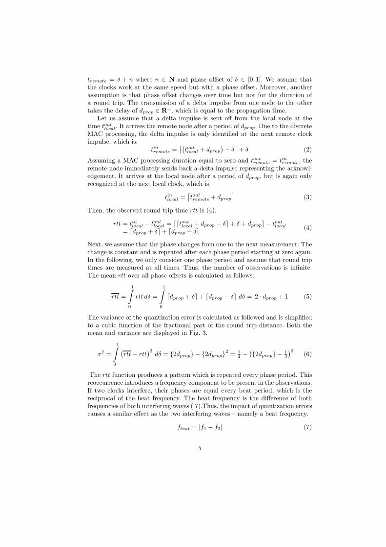
Next, we assume that the phase changes from one to the next measurement. Thechange is constant and is repeated after each phase period starting at zero again.In the following, we only consider one phase period and assume that round triptimes are measured at all times. Thus, the number of observations is infinite.The mean rtt over all phase offsets is calculated as follows.

rtt =

1∫

0

rtt dδ =

1∫

0

�dprop + δ� + �dprop − δ� dδ = 2 · dprop + 1 (5)

The variance of the quantization error is calculated as followed and is simplifiedto a cubic function of the fractional part of the round trip distance. Both themean and variance are displayed in Fig. 3.

σ2 =

1∫

0

(rtt − rtt

)2dδ = {2dprop} − {2dprop}2 = 1

4 − ({2dprop} − 12

)2 (6)

The rtt function produces a pattern which is repeated every phase period. Thisreoccurrence introduces a frequency component to be present in the observations.If two clocks interfere, their phases are equal every beat period, which is thereciprocal of the beat frequency. The beat frequency is the difference of bothfrequencies of both interfering waves ( 7).Thus, the impact of quantization errorscauses a similar effect as the two interfering waves – namely a beat frequency.

fbeat = |f1 − f2| (7)

5

323µs 324µs322µs 325µs

continuous interval [323µs,325µs[

discretedistribution as measured

real continuousdistribution as assumed

Fig. 2. Discrete distribution of noisy delaymeasurements.

0.0 0.2 0.4 0.6 0.8 1.0

0.0

0.5

1.0

1.5

2.0

2.5

3.0

Actual distance

Cal

cula

ted

dist

ance

and

var

ianc

e meanvariance

Fig. 3. Theoretical mean distance andvariance of distance.

Limits and Verification: The accuracy of location and distance sensing algo-rithms have fundamental limits (refer to the citation in [1]). For example, theanalytic calculations above do not take into account the clock drift during oneRTT observation. Assuming a frequency stability of ±25 ppm and a length ofa transmission sequence of 60 µs and 320 µs, the maximal error could be up to0.9 m and 4.8 m respectively.

Furthermore, one should note that only in vacuum light travels at the speedof light c. In materials the propagation speed depends on the square root ofthe dielectric constant ε. For example, dry ferroconcrete has an ε of about 9and electromagnetic waves traverse through ferroconcrete 3 times slower than invacuum. Most other materials used in buildings have lower dielectric constants.

Another source of possible errors is due to non-line-of-sight conditions. Thisresults in an overestimation of the distance between the two nodes [12]. Multi-path propagation might introduce measurement errors because the dominantpath can vary depending on the current transmission conditions. Multi-pathpropagation is only present if reflections are given. Reflections can have largeimpact on signal strength but only a low one on propagation delay. Thus, inthe presence of multi-path propagation or reflections, we assume time delaymeasurement as being more precise than those based on the RSSI.

In order to check these hypotheses and identify the real measurement resolu-tion, we conducted experiments. The first measurement campaign was conductedto study the impact of slow-user motion on packet loss and delay as describedin [10]. At the same time, we also measured the impact of distance on the roundtrip times. One year later, we embarked on a second measurement campaign.We altered the radio modem technology, the location, the analysis software, andthe staff. The consistence of both results proves the reliability and correctnessof our approach.

6

4 Measurements: First and second campaign

Experimental setup: The measurement was conducted twice: First in a gymna-sium [10] and later in the in the countryside where one could expect the channelto be free of disturbing noise coming from other radiating devices. The datacommunication took place between the local and the remote node. ICMP pingpackets were transmitted each 20 ms (A) respective 10 ms. The measurementsof RTT were conducted for several distances: First covering the range from 5 to40 m, later extend to the maximal transmission range of 100 m.

At each distance, we measured for about 15 minutes respective 4 minutes.One should note, that in this first campaign, the wireless LAN cards were sit-uated close to the ground. Also, the directions of the antennas were selected atrandom and were not recorded. This is important to know as it explains someof the results presented later. In the second session the sender was placed on aplastic table, whereas the receiver was installed on top of a 1.5 m wood-metalladder. This was to guarantee that a large percentage of the Fresnel-zone, anelliptic space around the direct line-of-sight between both nodes is free of anyobstacles harming the transmission. This time, the antennas were directed to-ward each other.

Equipment: The PCs were running a Suse 6.4 Linux system with a 2.4.17 kernel(A). D-Link cards featuring an Intersil’s (now Conexant) Prism2 chipset wereemployed as a wireless interface. Packets were directly sniffed on the MAC layerby the measurement tool ‘Snuffle’.

The second time, we used an access point (Netgear FWAG114) support-ing 802.11b/g as remote node. The PCs were running under Linux, Suse 9.1,with a special 2.6 kernel. We used two different WLAN cards containing chipsets from Atheros and Conexant implementing IEEE 802.11 a,b and g. TheAtheros cards (brand Netgear WAG-511, contained an AR5212 chip) are sup-ported by the Madwifi device driver. We used the software version downloadedfrom the CVS server on the August 30th, 2004. The Conexant cards (brand:Longshine LCS-8531G containing Prism-GT chipset with an ISL3890 as MAC-Controller) are controlled by the prism54.org device driver (date 28-06-2004,firmware 1.0.4.3.arm). During each measurement both the sender and monitorwere equipped with cards of the same brand. To gather the packet traces, weused tcpdump and libpcap.

Configuration: WLAN networking technologies based on the IEEE 802.11 stan-dards transmit data packets via air. To avoid potential packet delay effects, inthe first experiments the maximal number of retransmissions (transmission type)was set to zero. The second measurements were conducted in seven different con-figurations to study the impact of the WLAN card, CPU clock and modulationtype. We used the default configuration of WLAN cards and access point butchanged the supported standard to 802.11g and set the modulation type to ei-ther 36 or 54 Mbit/s. The frame length of the data packets are 65 bytes and ofthe acknowledgements 14 bytes.

7

Time measurements: All three different WLAN cards recorded the arrival timeof packets at a resolution of 1 µs without any variable latency. The precise pointof time, at which the time stamp is recorded, is not documented. Also, the WLANchip sets feature only the recording of time stamps of incoming packets. But weneeded both sending and receiving time stamps. Therefore, we decided to use athird PC to monitor the packets which the local node sends and receives. Themonitor PC was placed close-by the sender to avoid any additional propagationdelays that could falsify the measurements.

It will be straight forward to alter software and firmware of WLAN cards torecord transmission time stamps, too. Due to legal constraints, we were not ableto implement these changes by ourselves. We expect that WLAN chipset man-ufactures will provide firmware updates to support precise time stamps becausethey will benefit from customers using WLAN for location-aware services. Untilthen, we are required to use the third monitoring node.

Data collection & processing: Snuffle provides the packet traces of all 802.11bpackets received at the monitoring node. We filtered-out only the successful pingsequences which consist of an ICMP request, an acknowledgement, an ICMPresponse and again an acknowledgement. Other packets like erroneous transmis-sions, beacons, ARQ messages etc. were dropped. Due to hardware limitationsof the WLAN card only a fraction of observations were recorded.

Only the delays fitting in the interval [323 µs, 324 µs] are considered in furthercalculations (Fig. 2). A few delay measurements were observed with the valueof 322 and 325 µs. These and all other delays were considered as measurementerrors. Taken the valid packet sequences, the mean and variance of the remotedelay and local delay were calculated. To check for stationary process properties,the autocorrelation function was calculated.

In the second round, Tcpdump recorded the packet traces and wrote themto files. After the measurements we used tcpdump to convert these files to plaintext files. Tcpdump had to be modified in order to print out the prism link-layerheaders. For statistical analysis the R project software turned out to be quiteefficient. Thus, this time we applied R programs to calculate the data’s analyzedmean, variance and autocorrelation.

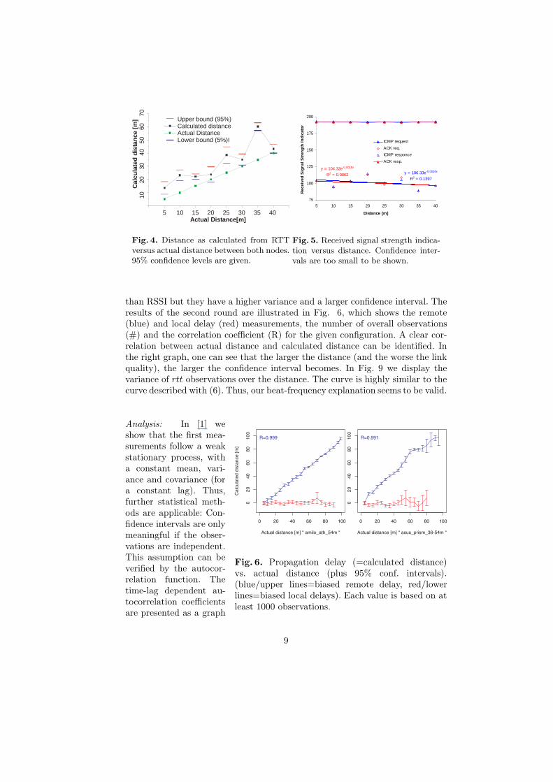
Results: The distance was directly derived from the measured propagation delayusing equation (1). Assuming a Gaussian error distribution, we also plotted theconfidence intervals in Fig. 4. In the first campaign the calculated distances werealways higher than the real distances. Also, in some measurements (e.g. 35 m)the air propagation time was significantly higher. Due to the experimental setup,we could not ensure that the direct line-of-sight path was taken. The remote nodewas placed directly on the ground. Thus, the Fresnel zone was violated and thedirect transmission path was hampered.

In Fig. 5 the signal strength is displayed as a function of the distance. Theo-retically, the signal strength should decrease with distance. In this measurementcampaign other factors, such as reflection, seem to be dominant. If one comparesFig. 4 and Fig. 5, it seems time measurements reflect the distance more precisely

8

5 10 15 20 25 30 35 40 Actual Distance[m]

Cal

cula

ted

dist

ance

[m]

10

20

30

4

0 5

0

60

70

Upper bound (95%)Calculated distanceActual DistanceLower bound (5%)I

Fig. 4. Distance as calculated from RTTversus actual distance between both nodes.95% confidence levels are given.

y = 106.33e-0.0024x

R2 = 0.1397

y = 104.32e-0.0019x

R2 = 0.0862

75

100

125

150

175

200

5 10 15 20 25 30 35 40

Distance [m]

Rece

ived

Sig

nal S

treng

th In

dica

tor

ICMP requestACK req.ICMP responceACK resp.

Fig. 5. Received signal strength indica-tion versus distance. Confidence inter-vals are too small to be shown.

than RSSI but they have a higher variance and a larger confidence interval. Theresults of the second round are illustrated in Fig. 6, which shows the remote(blue) and local delay (red) measurements, the number of overall observations(#) and the correlation coefficient (R) for the given configuration. A clear cor-relation between actual distance and calculated distance can be identified. Inthe right graph, one can see that the larger the distance (and the worse the linkquality), the larger the confidence interval becomes. In Fig. 9 we display thevariance of rtt observations over the distance. The curve is highly similar to thecurve described with (6). Thus, our beat-frequency explanation seems to be valid.

Fig. 6. Propagation delay (=calculated distance)vs. actual distance (plus 95% conf. intervals).(blue/upper lines=biased remote delay, red/lowerlines=biased local delays). Each value is based on atleast 1000 observations.

Analysis: In [1] weshow that the first mea-surements follow a weakstationary process, witha constant mean, vari-ance and covariance (fora constant lag). Thus,further statistical meth-ods are applicable: Con-fidence intervals are onlymeaningful if the obser-vations are independent.This assumption can beverified by the autocor-relation function. Thetime-lag dependent au-tocorrelation coefficientsare presented as a graph

9

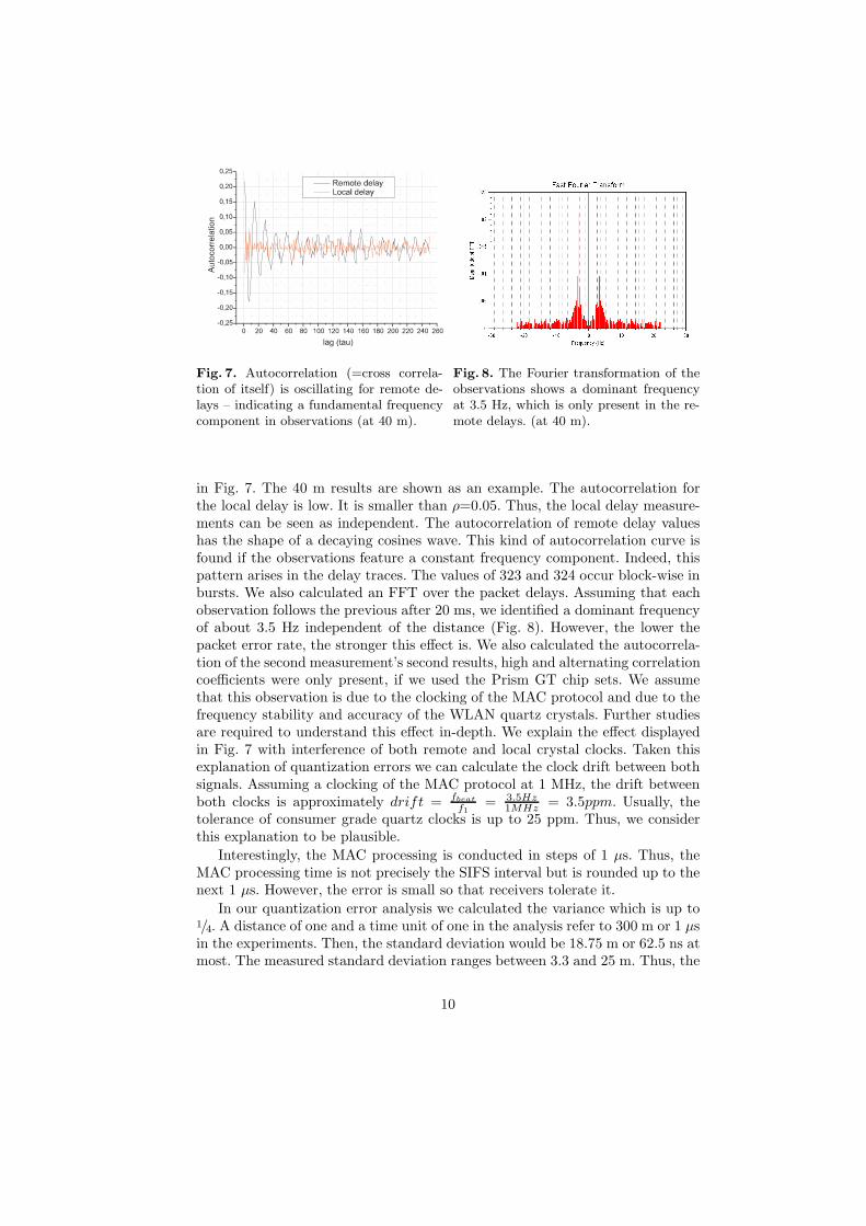
Fig. 7. Autocorrelation (=cross correla-tion of itself) is oscillating for remote de-lays – indicating a fundamental frequencycomponent in observations (at 40 m).

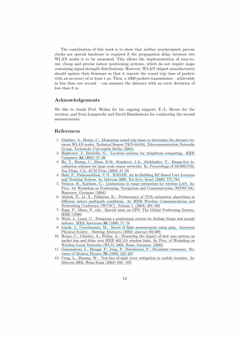
Fig. 8. The Fourier transformation of theobservations shows a dominant frequencyat 3.5 Hz, which is only present in the re-mote delays. (at 40 m).

in Fig. 7. The 40 m results are shown as an example. The autocorrelation forthe local delay is low. It is smaller than ρ=0.05. Thus, the local delay measure-ments can be seen as independent. The autocorrelation of remote delay valueshas the shape of a decaying cosines wave. This kind of autocorrelation curve isfound if the observations feature a constant frequency component. Indeed, thispattern arises in the delay traces. The values of 323 and 324 occur block-wise inbursts. We also calculated an FFT over the packet delays. Assuming that eachobservation follows the previous after 20 ms, we identified a dominant frequencyof about 3.5 Hz independent of the distance (Fig. 8). However, the lower thepacket error rate, the stronger this effect is. We also calculated the autocorrela-tion of the second measurement’s second results, high and alternating correlationcoefficients were only present, if we used the Prism GT chip sets. We assumethat this observation is due to the clocking of the MAC protocol and due to thefrequency stability and accuracy of the WLAN quartz crystals. Further studiesare required to understand this effect in-depth. We explain the effect displayedin Fig. 7 with interference of both remote and local crystal clocks. Taken thisexplanation of quantization errors we can calculate the clock drift between bothsignals. Assuming a clocking of the MAC protocol at 1 MHz, the drift betweenboth clocks is approximately drift = fbeat

f1= 3.5Hz

1MHz = 3.5ppm. Usually, thetolerance of consumer grade quartz clocks is up to 25 ppm. Thus, we considerthis explanation to be plausible.

Interestingly, the MAC processing is conducted in steps of 1 µs. Thus, theMAC processing time is not precisely the SIFS interval but is rounded up to thenext 1 µs. However, the error is small so that receivers tolerate it.

In our quantization error analysis we calculated the variance which is up to1/4. A distance of one and a time unit of one in the analysis refer to 300 m or 1 µsin the experiments. Then, the standard deviation would be 18.75 m or 62.5 ns atmost. The measured standard deviation ranges between 3.3 and 25 m. Thus, the

10

Fig. 9. The variance of rttobservations over time.

Fig. 10. The accuracy (cross correlation and standarderror) over the number of observations per position.

quantization error is not the only dominant effect and others such as thermalnoise are important too.

We measured at each distance for 4 to 15 minutes. Is it really required tomeasure that long? In Fig. 10 we consider only a subset of all rtt observationstaken during the second campaign. We display the correlation coefficient R andthe standard error over the number of observations per distance. With 500 to1000 observations per position nearly the optimal accuracy is achieved. If oneassumes that a packet is sent off every mircosecond, the distance can be estimatedafter 1 s of continues transmission.

5 Conclusion

We have presented an algorithm to measure the air propagation time of IEEE802.11 packets with a higher accuracy. Using two different experimental setups,we determined the precision of round trip time measurements. We used com-mercial WLAN cards, supporting IEEE 802.11b and 802.11g, implemented withthree different WIFI chip sets. We have shown that such time measurementsare possible even with off-the-shelf, commercial WLAN equipment and withoutadditional signal processing hardware.

To overcome the low resolution of the clocks, numerous observations have tobe combined and smoothened. This can be carried out best during an ongoingdata transmission at no additional cost. We explained why smoothing indeedhelps to enhance the resolution of the time difference measurement so that dis-tance measurements become possible. This effect can be due to the presence ofmeasurement noise and to the beat frequency resulting from drifting clocks. Tothe best of our knowledge, especially the latter explanation is novel.

Our finding suggests that instead of RSSI the round trip time should be mea-sured because it is correlated with the distance more strongly. In our gymnasiummeasurement the RSSI has not been useful to identify the distance because –due to reflections – the attenuation varied largely.

11

The contribution of this work is to show that neither synchronized, preciseclocks nor special hardware is required if the propagation delay between twoWLAN nodes is to be measured. This allows the implementation of easy-to-use, cheap and precise indoor positioning systems, which do not require mapscontaining signal strength distributions. However, WLAN chipset manufacturersshould update their firmware so that it reports the round trip time of packetswith an accuracy of at least 1 µs. Then, a 1000 packets transmission – achievablein less than one second – can measure the distance with an error deviation ofless than 8 m.

Acknowledgements

We like to thank Prof. Wolisz for his ongoing support, E.-L. Hoene for therevision, and Sven Lamprecht and David Hundenborn for conducting the secondmeasurements.

References

1. Gunther, A., Hoene, C.: Measuring round trip times to determine the distance be-tween WLAN nodes. Technical Report TKN-04-016, Telecommunication NetworksGroup, Technische Universitat Berlin (2004)

2. Hightower, J., Borriello, G.: Location systems for ubiquitous computing. IEEEComputer 34 (2001) 57–66

3. He, T., Huang, C., Blum, B.M., Stankovic, J.A., Abdelzaher, T.: Range-free lo-calization schemes for large scale sensor networks. In: Proceedings of MOBICOM,San Diego, CA, ACM Press (2003) 81–95

4. Bahl, P., Padmanabhan, V.N.: RADAR: An In-Building RF-Based User Locationand Tracking System. In: Infocom 2000, Tel-Aviv, Israel (2000) 775–784

5. Velayos, H., Karlsson, G.: Limitations in range estimation for wireless LAN. In:Proc. 1st Workshop on Positioning, Navigation and Communication (WPNC’04),Hannover, Germany (2004)

6. Alsindi, N., Li, X., Pahlavan, K.: Performance of TOA estimation algorithms indifferent indoor multipath conditions. In: IEEE Wireless Communications andNetworking Conference (WCNC). Volume 1. (2004) 495–500

7. Enge, P., Misra, P., eds.: Special issue on GPS: The Global Positioning System,IEEE (1999)

8. Werb, J., Lanzl, C.: Designing a positioning system for finding things and peopleindoors. IEEE Spectrum 35 (1998) 71–78

9. Lepak, J., Crescimanno, M.: Speed of light measurement using ping. AmericanPhysical Society - Meeting Abstracts (2002) abstract B2.009.

10. Hoene, C., Gunther, A., Wolisz, A.: Measuring the impact of slow user motion onpacket loss and delay over IEEE 802.11b wireless links. In: Proc. of Workshop onWireless Local Networks (WLN) 2003, Bonn, Germany (2003)

11. Gammaitoni, L., Hanggi, P., Jung, P., Marchesoni, F.: Stochastic resonance. Re-views of Modern Physics 70 (1998) 223–287

12. Cong, L., Zhuang, W.: Non-line-of-sight error mitigation in mobile location. In:Infocom 2004, Hong Kong (2004) 650– 659

12