Measuring Productivity Change for Regulatory Purposes

Measuring Productivity Change for Regulatory Purposes

D. Mark Kennet1

and

Noel D.Uri2,3

1    ? George Washington University.2    ? Federal Communications Commission.3    ? The views expressed are those of the authors and do not necessarily represent the policies of the organizations with which they are affiliated. The authors would like to thank two anonymous referees for useful suggestions.

Abstract

Incentive regulation for local exchange carriers in the telecommunication industry in the United States for some of the

services they provide is based on price caps. Under price caps,a regulated firm?s average real prices for services it provides are

required to fall by a specified percentage each year. This percentage is known as the X-factor. An important component of the X-factor is productivity change for local exchange carriers providing interstate access service. Two separate approaches to measuring the change in productivity are considered. The total factor productivity approach, which is currently used in regulatory proceedings in the telecommunications industry, quantifies the change in output less the change in input and classifies it as the measure of productivity growth. There are anumber of limitations with this approach. An alternative is proposed, the hybrid cost proxy model, which is an engineering process model that does not possess the limitations of the total factor productivity approach. The model combines engineering principles of design for the local loop, switching and interoffice networks with economic principles of cost minimization. The two separate approaches are empirically implemented for Bell Atlantic, Inc. ? Maryland for the period 1985 to 1997. The results suggest that the realized productivitygrowth as measured by the total factor productivity approach is somewhat less than what would have been achieved had the network been optimally configured as indicated by the hybrid cost proxy model approach.

1

IntroductionIncentive regulation has been adopted in the

telecommunications industry in the United States by the Federal Communications Commission (Crew & Kleindorfer, 1996 and Kridel etal., 1996). Incentive regulation is typically defined as the implementation of rules that encourage a regulated firm to achieve desired goals by granting some, but not complete, discretion to the firm. Three aspects of this definition of incentive regulation are important. First, regulatory goals mustbe clearly specified before incentive regulation is designed. The properties of the best incentive regulation plan will vary according to the goals the plan is designed to achieve. Second, the regulated firm is granted some discretion under incentive regulation. For example, while the firm may be rewarded for reducing its operating costs, it is not told precisely how to reduce these costs. Third, the regulator imposes some restrictions on relevant activities or outcomes under incentive regulation (Bernstein & Sappington, 1999).

One popular incentive regulation plan is the price cap plan.The central idea behind price cap regulation is to control the prices charged by the regulated firm, rather than its earnings. Essentially, price cap regulation plans require the regulated firm?s average real prices to fall annually by a specified percentage (Mitchell & Vogelsang, 1991). This percentage is

2

nominally referred to as the ?X-factor? or the productivity offset.

In the case of incumbent local exchange carriers (LECs) regulated by the Federal Communications Commission, a price cap index (PCI) for interstate access is adjusted annually according to the PCI relationship defined in the Code of Federal Regulations.4 The price cap index consists of a measure of inflation,

in this case the Gross Domestic Product Price Index (GDP-PI),minus the X- factor,plus or minus any permitted exogenous cost changes.

For LEC interstate access service,it was argued in 1995that applying price cap regulation allows the Federal Communications

Commission,as closely as possible,to replicate the effects of a competitive market. That is,competition should be the model for

setting just and reasonable LEC rates based on a PCI because ?Effective competition encourages firms to improve their productivity and introduce improved products and services, in order to increase their profits. With prices set by marketplace forces, the most efficient firms will earn above-average profits,while less efficient firms will earn lower profits, or cease operating. Over time, the benefits of competition flow to customers and to society, in the form of prices that reflect costs, maximize social welfare, and efficiently allocate

4    ? Section 61.45 (b) of the Federal Communications Commission?s rules.

3

resources.?5

In the Price Cap Performance Review for Local Exchange Carriers,6 it was noted that changes in a firm'scosts of producing a

unit of output are the product of both changes in the quantity of inputs used and changes in the prices paid for those inputs. It was concluded that the X-factor should include both a measure of productivity growth

and a measure of input price change. A total factor productivity (TFP) approach was adopted for deriving the productivity component of the X-

factor. The other component of the X-factor is an input price differential. A number of very explicit assumptions underlie TFP

analyses. In particular,the conventional growth accounting method of measuring TFP of firms is to assume that there are constant returns to

scale and that observed inputs and outputs have been generated by firms in competitive,long run equilibrium. With prices of output and inputs

fixed,the firm chooses input levels so as to maximize profit (Berndt & Fuss,1986and Jorgenson & Griliches,1967).The measure of TFP growth

obtained by conventional means is not,however,appropriate whenever firms are not in a long run cost minimizing equilibrium. A firm is not in

long run equilibrium whenever the firm'sinput-output bundle is other than corresponding to a point on the long run unit cost curve. If the firm is not in long run equilibrium,then profit is not zero.

Limitations on the Current Approach to Price Cap Regulation

5    ? Price Cap Performance Review for Local Exchange Carriers (10 FCC Rcd at 9002).6    ? 10 FCC Rcd at 9033 (paras. 160-61).

4

In choosing a price cap index (PCI),price cap regulation should set a maximum price depending on factors exogenous to the firm,such as

factor prices or regional incomes.7 In practice,as it has evolved at the Federal Communications Commission,the PCI is determined based on LEC specific data.

The most important argument against the use of the firm?s own data for computing the TFP is that it is not incentive compatible. That is, because the disaggregated input and output data are under the control of the regulated firm, they are subject to manipulations (Kiss, 1991) and/or to misrepresentationof the true state of affairs. For example, after price caps for interstate access went into effect in 1991, most LECs reduced employment levels dramatically. These labor force reductions were achieved by offering employees monetary incentives to leave the company. There is some variability in the applicable accounting rules, but these payments were generally accrued as one-time charges against current earnings. This inflates costs in the early years of the price cap implementation and, consequently, biases measures of TFP growth downward.

A second concern with using firm-specific data to compute TFP is that past productivity changes are not necessarily a good measure of future productivity changes especially in the

7    ? The discussion here focuses on the efficient use of inputs. The economic properties of output choices are not explicitly considered since the concern is on just the interstate access market.

5

telecommunications industry were rapid deployment of new technology including such things as frame relays, ATM (asynchronous transfer mode), and optical fiber is taking place. Each of these investments serves to affect significantly TFP. One of the striking characteristics of annual changes in TFP is their considerable temporal variability. For example, as reported in the Fourth Report and Order in CC Docket No. 94-1 of the Federal Communications Commission, average TFP for the Regional Bell Operating Companies between 1986 and 1995 is 2.94 with a variance of 7.27. Great variation in time makes it difficult or impossible to choose an appropriate historical TFP change for the PCI.8

Another general bias introduced in the measurement of TFP of LECs is associated with the use of LEC performance data immediately post-

divestiture. This will bias downward the measure. It is generally conceded that under rate-of-return (ROR)regulation,regulated firms employed too much capital and too much labor (Averch & Johnson,1962and

Sherman,1992).Transition from the regulated environment is not instantaneous. The optimal level of factors of production will be in

8    ? Note that the temporal variability in TFP is a solely a function of changes in the underlying measures including output and inputs. This has obvious implications for setting price caps. Basedon LEC TFP for a single year or a small number of years, price caps would be very unstable. Hence, price caps are based on a average over the entire historical period for which data are available. For more on this, see Price Cap Performance Review for Local Exchange Carriers (10 FCC Rcd).

6

disequilibrium for some period of time following the demise of ROR regulation. Hence,the measured TFP will contain some disequilibrium

periods.9 That is,the measurement of the productivity of LECs is necessarily calculated,at least partially,in a ROR environment which

will bias downward the measured TFP for at least a portion of theperiod.

A final general bias introduced in the measurement of TFP is associated with the demand for interstate access to local LECs'local

loops. Interstate access service is the focus of price cap regulation. It has grown much more rapidly on average than demand for local service

and intrastate access service. The data on this are clear. Thus,in the presence of economies of density,this leads to the conclusion that TFP

in interstate services has grown faster than company-wide (regulated) TFP. More specifically,the PCI being considered here applies to

interstate access services but TFP is commonly computed based on all LEC services. There is every reason to expect that productivity

enhancements experienced historically in the interstate access market would be substantially greater than the overall rate of

9    ? As noted previously, an important assumption underlying any computation of TFP is that all inputs (factors of production) are in full static equilibrium. In many instances for local exchange carriers, however, the assumption of full static equilibrium is suspect and hence, so are the empirical results. Additionally, departures from full static equilibrium may result from factors otherthan internal adjustment costs. In the case of LECs, there is no evidence that capital stocks, for example, are completely adjusted atall times to cost-minimizing levels.

7

productivity growth experienced by LECs in supplying all services. Most of the productivity growth experienced in the telecommunications

industry is related to reductions in switching costs and to savings in transmissions costs which occur as a result of using electronics to

expand the carrying capacity of transmissions facilities. In contrast productivity growth in supplying loop services has been relatively

lower. As a result,the average measure of TFP used in setting the X- factor,and which should properly reflect productivity growth in the

interstate access market,is biased downward. The bottom line is that use of a conventional growth accounting

total factor productivity approach for deriving the productivity component of the X-factor used in setting the price cap index has a

number of significant limitations. Some of the problems are endemic to the TFP approach and cannot be effectively dealt with. Thus,there

clearly exists a need to find an alternative approach. This is the subject of what follows.

A Hybrid Cost Proxy Model (a)Introduction

Engineering process models have been developed in recent years as an alternative to the TFP approach to productivity measurement.

Engineering process models offer a more detailed view of cost structures than is possible using the traditional TFP approach. In

addition engineering process models are better suited for modeling forward-looking (long run)costs since they rely much less on historical

8

data than the TFP approach. They enable regulatory authorities to estimate forward-looking costs (i.e.,the expected future costs)of

network facilities and services without having to rely on detailed cost studies prepared by incumbent local exchange carriers (Gasmi et

al.,1999).In this context,they can be used for determining the forward- looking cost of network elements involving the measurement of

productivity changes. Engineering process models typically consist of several

components. A cluster algorithm performs the first level of network design by grouping customers into serving areas. Thus,loop plant can

be designed to reach individual customer locations as determined from geocoded location data. Next,a cost minimization objective function

is used in loop plant design. Thus,for example,a feeder or distribution network is selected by weighing the benefits of minimizing total route

distance (andhence cost structure)and minimizing total cable distance (andconsequently cable investment and maintenance costs).

Such models attempt to optimize the trade-off between distribution plant,feeder plant,and loop design by considering alternative

configurations of the distribution plants for the network. Customers can be located closer to a serving area interface,but at a cost of

additional feeder plant and loop electronics. There are also switching,interoffice,and expense components.

Switching costs are estimated using host-remote data. The interoffice component estimates the cost of interconnection between host and

9

tandem10 switches. The expense component converts investment into an estimate of the monthly cost of providing service. Expenses include

plant-specific expenses such as maintenance of facilities and equipment expenses,plant non-specific expenses,such as engineering,

network operations,and power expenses,customer service expenses such as marketing,billing,and directory listing expenses,and corporate

expenses such as administration,human resources,legal,and accountingexpenses.

In what follows an engineering process model will be discussed that determines the forward-looking cost (i.e.,the expected future cost)

of network elements. These costs can then be used to measure the expected change in productivity. The Federal Communications

Commission'sHybrid Cost Proxy Model (HCPM)11 and the Synthesis Model (SM)will be used. A demonstration of its applicability using customer

location data from Bell Atlantic ? Maryland, Inc. (formerly, the C and P Telephone Company of Maryland) will be conducted. The discussion is organized as follows: In the next section, the HCPMand SM and their salient features for productivity measurement are described followed by a discussion of productivity measurement. The approach is applied and the results compared tothe results of a TFP analysis. The final section looks at the

10    ? A tandem switch connects one trunk to another. A tandem switch is an intermediate switch or connection between an originatingcall location and the final destination of the call.11    ? A complete description of the model can be found in Bush et al. [1999.

10

advantages and limitations of the two approaches.(b) The Hybrid Cost Proxy Model and Synthesis Model

The model presented here was originally developed as an alternative to models being promoted by telecommunications industry groups in a variety of regulatory settings (Bush et al.,1999). The model combines principles of engineering design for the local loop, switching and interoffice networks with economic principles of cost minimization. Because it draws freely from engineering principles displayed in other models, is called the Hybrid Cost Proxy Model, or HCPM.

The HCPM currently consists of two independent components ? a customer location component and a loop design component. The customer location component first groups individual geographic locations of telephone customers into clusters, based on engineering considerations. Next, the customer location component determines a grid and microgrid overlay for each cluster, and places each customer location into the correct microgrid cell. The loop design component determines the total investment required for an optimal distribution and feeder network by building loop plant to designated customer locations represented by populated microgrid cells. The number of microgrids in a grid can vary from 4 to 2500. When used with a source of geocoded customer locations and a maximum copper wire reach of 18,000 feet, a uniform microgrid size of 360 feet can be

11

maintained. All customer locations can therefore be determined with an error of not more than several hundred feet.

For the purposes of completing the calculation of cost of a network, the Federal Communications Commission staff integrated portions of the HAI model proposed by AT&T and MCI-WorldCom.12

These portions include the calculation of switching investment, signaling investment,and interoffice trunk investment,as well as a component for converting investments into annual expenses. The resulting integrated model is called the Synthesis Model,or SM (Le&

Sharkey,1998). (i)The Customer Location Component The objective is to estimate the cost of building a telephone

network to serve subscribers in their actual geographic location,to the extent these locations are known. The estimate of the cost of

serving the customer within a given wire center'sboundaries includes the calculation of switch size,the length,gauge,and number of copper and fiber cables,and the number of DLCs (digital loop carrier)required.

These factors depend,in turn,on how many customers the wire center serves,where customers are located within the wire center's

boundaries,and how customers are distributed within neighborhoods. Particularly in rural areas,some customers may not be located in

neighborhoods at all but,instead,may be scattered throughout outlyingareas.12    ? HAI denotes Hatfield Associates, Inc. It is the firm hired by AT&T and MCI-WorldCom to develop this model.

12

Once customer locations have been determined,a cluster algorithm is employed to group customers into serving areas in an efficient

manner that takes into account consideration of relevant engineering constraints (Gower & Ross,1969).The approach is designed to accept as

input a set of geocoded locations for every customer. It then performs a rasterization procedure13 which assigns customers to microgrid cells.

The cluster algorithm then groups the sets of raster cells into natural clusters. Finally,a square grid is constructed on top of every cluster,

and all customer locations in the cluster are assigned to a microgrid cell for processing by the loop design component.

(ii)Design of Distribution and Feeder Plants A telephone network must allow any customer to connect to any

other customer. To accomplish this,a telephone network must connect customer premises to a switching facility (wire center),ensure adequate capacity exists in that switching facility to process all

customers'calls that are expected to be made at peak periods,and then interconnect that switching facility with other switching facilities

to route calls to their destinations. Within the boundaries of each wire center,the wires and other equipment that connect the central

office to the customers'premises are know as outside plant. Outside plant can consist of either copper cable or a combination of optical fiber and copper cable as well as associated electronic equipment.

13    ? A raster is simply a grid covering the entire wire center. One point in each cell of the grid is used to represent all of the customer locations that fall in that cell.

13

Copper cable generally carries an analog signal that is compatible with most customers'telephone equipment. Optical fiber cable carries

a digital signal that is incompatible with most customers'telephone equipment,but the quality of the signal carried on optical fiber is

superior at greater distances when compared to a signal carried on a copper wire. Generally,when a customer is located too far from the wire center to be served by copper cables alone,an optical fiber will be

deployed to a point near the customer where the digital light signal carried on the optical fiber cable will be converted to an analog

signal that is compatible with the customer'stelephone. The conversion is carried by a digital loop carrier remote terminal (DLC)

which is connected to a serving area interface (SAI).The portion of the loop plant that connects the central office with the SAI or the DLC is

known as the feeder plant,and the portion that runs from the DLC or the SAI throughout the service area is known as the distribution plant.

Given the inputs from the customer location component,the logic of the loop design component is straightforward. Within every

microgrid with non-zero population,customers are assumed to be uniformly distributed. Each populated microgrid is divided into a

sufficient number of equal sized lots and distribution cable is placed to connect every lot. These populated microgrids are then connected to

the nearest concentration point (SAI)by further distribution plant. The SAIs are connected to the central office by feeder cable. On every

link of the feeder and distribution network,the number of copper or

14

optical fiber lines and the corresponding number of cables are explicitly computed. The total cost of the loop plant is the sum of the

costs incurred on every link. Distribution consists of all outside plant between a customer

location and the nearest SAI. Distribution plant consists of backbone and branching cables where branching cables are closer to customer

locations. Feeder consists of all outside plant connecting the central office main distribution frame to each of the SAIs. The distribution

portion of the loop design component determines the cost of distribution plant for each cluster independent of information about

neighboring clusters. (iii)Switching and Signaling Investment Component,Interoffice Component,and Expense Component.

A very simplified model of switch investment is used. Investment is just a linear function on the number of access lines.

The interoffice component models a SONET14 ring interoffice network connecting all switches in a serving area. First,host-remote

relationships are taken into account,and host-remote rings are formed. Hosts and stand alones are then joined in a cost-minimizing ring,taking

into account the capacity of interconnecting links based on traffic at each switch.

14    ? Synchronous Optical NETwork (SONET) is a family of fiber optic transmission rates from 51.84 million bits per second to 13.27 gigabits per second created to provide the flexibility needed to transport many digital signals with different capacities, and to provide a design standard for manufacturers.

15

The expense component develops an annual cost per dollar of investment based on known cost of capital,a depreciation schedule for

each component,and given operation and maintenance costs. Total operating expenses are calculated by summing investment-related

expenses with overhead and line-related expenses. The Productivity Change of a Local Exchange Carrier

Turn now to the empirical implementation of the productivity measures. Bell Atlantic,Inc. ? Maryland15 is selected as the service

area for study. It is the primary provider of local telephone service in Maryland.16 In 1997it had a total of 3,889,962access lines,and

handled 11,983,576local calls,153,253intraLATA toll calls,and 2,087,724 interLATA toll calls. For this same period,it had 52,581,237kilometers

of metallic wire in cable and 532,727kilometers of fiber in cable in conjunction with 258 central office switches and 50,902basic rate ISDN

control channels. Total operating revenues in 1997were $2,035,794,000 with total operating expenses of $1,419,703,000.In terms of total

operating revenue,it is the fifteenth largest local exchange carrier in the United States.

The period of interest is 1985to 1997. The year 1985is chosen because it is the year immediately following the breakup of AT&T. The

15    ? This was formerly known as the C and P Telephone Company of Maryland. It was one of the 22 local phone companies that was transferred to seven Regional Bell Operating Companies as a result ofthe breakup of AT & T in 1984.16    ? The other telephone service provider in Maryland in 1997 wasArmstrong Telephone Company ? Maryland. It is relatively small with just 6315 access lines in 1997.

16

year 1997is selected because it is the most recent period for which all of the requisite data are available. (a)The Total Factor Productivity (TFP)Approach

(i) Data Consistent with the typical requirement in regulatory

proceedings,the data used in the TFP analysis are taken solely from publicly available sources. The primary source of data in computing

the TFP between 1985and 1997is Statistics of Communications CommonCarriers (Federal Communications Commission,1985,1997/1998).Other

data are acquired from the Bureau of Economic Analysis and the Bureau of Labor Statistics.

From the Statistics of Communications Common Carriers ,data on the number of access lines (switched and special non-switched)for Bell

Atlantic,Inc. ? Maryland were obtained. These data are used as the measure of output. Between 1985 and 1997, output (the first component of the TFP measure) increased at an annual rate of 4.0%per year.

Computation of the input component of the TFP measure is considerably more complicated. Three inputs are considered labor, materials, and capital. Labor consists of the number of employees. While this is not the most desirable measure of labor, it is the only one that is publicly available. Between 1985 and 1997, the labor input declined by 3.2% per year.

Materials quantity is derived by dividing materials expense

17

by a materials price index. Materials expense for 1985 must be adjusted for two accounting changes that became effective in 1988. First, beginning in 1988 all expenses from nonregulated services that had joint and common costs with regulated services were reported in operating expenses. Second, certain plant investments that were formerly capitalized began to be expensed in the year they were incurred. Accordingly, 1985 expenses were adjusted upward to put them on a basis comparable to the accounting expense recorded for 1997. Materials expense, then, is just total adjusted operating expense minus the sum of total labor compensation, depreciation and amortization expense. Materials expense is divided by a materials price index to obtainmaterials quantity. The materials price index was obtained from the Bureau of Labor Statistics and is based on materials purchases of communications industries. Materials quantity increased at a 2.4% annual rate between 1985 and 1997.

Capital quantity is based on a perpetual inventory model (Goldsmith, 1951). Book value of total plant in service is used as the basis for calculating the benchmark (initial level) for capital stock. The benchmark year is 1985. In order to calculate constant dollar investment, chained Fisher asset pricesfrom the Bureau of Economic Analysis were used to deflate capitaladditions. Because of the 1988 capital/expense shift, end of year total plant in service less accumulated depreciation is

18

adjusted. Given this, the benchmark capital stock is derived using the Federal Communications Commission accounting relationship whereby total plant in service at the beginning of the year plus capital additions less capital retires equals totalplant in service at the end of the year. The depreciation rate used in the perpetual inventory model is calculated as the average depreciation equal to depreciation accruals divided by the average total plant in service at the beginning of the year and the total plant in service at the end of the year. Between 1985 and 1997, the capital quantity increased by 3.2% annually.

The changes in the three input quantities can be aggregated to yield a composite measure for the change in inputs. To do so requires information on each factor?s share of total costs. The payment to labor is total compensation, the payment to materials is materials expense, and the payment to capital is property income. Property income is computed following TFP conventions (Berndt and Fuss, 1986). Property income is defined simply as revenue less labor compensation less materials expense.

The aggregate input quantity is then labor input times laborshare of total costs plus materials quantity times materials share of total costs plus capital quantity times capital share oftotal costs. Between 1985 and 1997, the input quantity increasedby 1.3% annually. This is the second component of the TFP measure.

19

(ii) ResultsCombining the two TFP components indicates that productivity

of Bell Atlantic, Inc. ? Maryland increased at an annual rate of 2.7% between 1985 and 1997. This is substantially greater than the 0.3% experienced by the economy as a whole over the same period (Bureau of Labor Statistics, 1999). It is less, however, than the 3.7% rate realized by other local exchange carriers (AT&T, 1998).(b) The HCPM Approach

(i) DataIn the HCPM approach to the estimation of productivity

change due to technological innovation, the number and location of telephone customers in the region of interest is taken as given. Input prices dated 1997 are used for one cost optimization solution. Then, input prices dated 1985 are substituted for a second optimization solution. This approach issomewhat analogous to the index method commonly used (Deaton and Muellbauer, 1980). Prices for 1985 are estimated using the telecommunications industry-standard Turner price index applied to the actual 1997 prices (Spragins, 1991).17 It is assumed that

annual expense factors remain constant during the time period. Productivity change over the 1985to 1997period is then defined as the

absolute value of the difference between the natural logarithm of the

17    ? This is available at http://www.fcc.com.

20

annual cost in 1997less the natural logarithm of the annual cost in 1985divided by twelve.

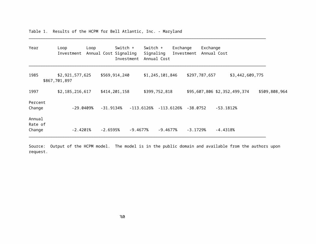
(ii) Results The results of the HCPM for Bell Atlantic,Inc. ? Maryland are

found in Table 1. Note that overall productivity growth is givenin the lower right-most entry. This value, 4.43%, can be broken down into two separate components: switching and signaling costs and outside plant excluding interoffice investment costs.

Interoffice investment costs are not included in the calculations for several reasons. First, while SONET ring technology is probably the forward-looking technology of choice today, it is unclear that telephone companies in the middle 1980swere contemplating this option as the efficient solution. This points up a limitation, which will be discussed later, in this approach. Namely, as in any modeling exercise involving technological innovation and capital stock, assumptions must be made regarding what constitutes the ?state of the art? in technology and, perhaps more importantly, what is the expected life of that technology. Another reason for ignoring interofficecosts for this analysis is that the total annual cost of transport in 1997 was $28,425,268, or only about 5.2% of total exchange cost.

Having the ability to separate loop cost from switching and signaling cost leads to policy inferences that deserve some

21

attention. First, note that the relatively slow productivity growth in loop investment is not unexpected. It is difficult to believe that great changes in the cost of investment in loop plant in this relatively labor-intensive activity have occurred. The HCPM results reflect this. While the model is capable of exploiting changes in the relative costs of technologies employedin the loop by optimizing and thus substituting, the major technological advance that has taken plant in the loop is digitalization. This is only really relevant when considering the serving area to the central office. Distribution plant, which the model estimates required $1,043,760,818 in investment for 1997, was approximately half of all loop investment.

Second, the relatively slow productivity growth in loop plant investment has a more subtle implication. It suggests thatthe political issues associated with universal service will remain important, at least until the bandwidth problems associated with wireless solutions are solved (Dodd, 1997). The reason for this is that the productivity enhancements that are observed, and that the model correctly notes, are in those portions of the network where ?fat pipes? are present. That is, those links in the network with relatively high capacity connecting relatively large demand nodes, such as switches and large commercial locations, realize the largest productivity change. The remainder of the network, including the overwhelming

22

majority of residential demand, is connected with much lower capacity links which, as was noted above, are declining in cost at a much slower rate. Thus, the relative cost of these more dispersed links will actually rise over time, although it may continue to decline in absolute terms.

Even if attention is paid only to the so-called last mile, it appears that business customers will enjoy some cost advantage, assuming rates are sufficiently deaveraged that they reflect the actual cost differentials. The results of reoptimizing the Bell Atlantic, Inc. - Maryland network under theassumption that only business and residential customers are present indicates that while productivity in the business only loop grows at a 3.6% annual rate over the twelve year period, productivity in residential lines grows by only 2.4%.18

This result most likely reflects the fact that business locations tend to be concentrated fairly closely in the general area of the wire

center,while residential locations are far more dispersed. Thus,the business locations are able to exploit the changing economics of

network design more readily than the residential locations. A final implication of the HCPM results pertains to less

developed countries and those with telephone line penetration significantly lower than that of the United States. It is anticipated

that a productivity change calculated using the HCPM is likely to be18    ? Complete results of this analysis are available from the authors upon request.

23

larger for such countries,since distribution facilities make up a much smaller proportion of the total network physical plant.

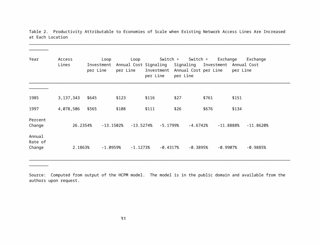
Turn now to productivity change attributable to economies of scale. Table 2 shows results of a hypothetical experiment using HCPM in which the network demand is assumed to increase by 30% from 1985to 1997. While it was not appropriate to assess productivity change in Table 1

as change in cost per line,19 here it is more reasonable to do so. The lower right hand entry in Table 3 shows that scale economies result in

an overall productivity increase of about 1%,or about half the annual rate of growth assumed in the number of access lines.

A Comparison of the TFP and the HCPM Approaches to ProductivityMeasurement

Both the TFP approach and the HCPM approaches presented here possess some limitations on their usefulness that pose problems in a

policy setting. A number of these have previously been noted. In addition,a limitation that all the approaches share is the treatment

of the dynamically evolving telecommunications network. The HCPM approach implicitly assumes that the network is rebuilt "from scratch"

each time the model is run.20 On the other hand,the TFP approach requires

19    ? Actually, the calculations would have remained identical butfor pedagogical purposes, it is best to consider efficiency over the entire network.20    ? This is the antithesis of the "scorched node" approach typically used in TELRIC pricing. There is an ongoing discussion as to which assumption is more appropriate. This discussion is long andcontentious. It will not be addressed here. The interested reader is referred to Iowa Utilities Board v FCC, No 96-3321, U.S. Court of

24

the use of data from periods very dissimilar to the current one. In the context of the rapidly changing technology in the telecommunications

industry,the results of the TFP can be severely misleading.21

Given this shortcoming with the conventional TFP approach,HCPM provides an advantage in that it obtains an optimal solution. It is possible to use the HCPM to calculate the costs associated with an

optimal static network at various points in time in order to approximate dynamic conditions. In using the HCPM approach,it is

probably best to choose a time interval consistent with a possible rebuilding of the network,as is done here,rather than choose very

short intervals. The TFP approach has a clear advantage in terms of data

availability. The forward-looking investment data necessary to use the HCPM can be difficult and time consuming to collect.

On the other hand,there are significant advantages to using the HCPM approach in the context of calculating an X-factor. First,the cost

model can be thought of as setting a benchmark for approximating ?ideal? productivity attainable by the LEC. Thus, a realistic

Appeals for the 8th Circuit, July 18, 2000 together with the voluminous record. Note that TELRIC pricing is currently used by allstates in setting UNE (unbundled network element) prices in accordance with the Telecommunications Act of 1996.21    ? It is important to note that the factors that lead to the variability in measured TFP will not impact the productivity measure from the HCPM approach. TFP uses historical data on output and inputs while the HCPM approach relies on forward-look cost data which, by their nature, demonstrate much less variability.

25

incentive structure is established under which a LECs? price ceiling reflects what an efficient firm would attain in an environment of rapid technological change and not what the average LEC attained over the historical period.

Perhaps even better, the HCPM captures the specific physicalattributes associated with each wire center. Thus, X-factors canbe LEC-specific and still be used as an independently determined benchmark.

Finally, the cost function approach suffers none of the common problems of aggregation (Griliches, 1986). Among these problems is that aggregate (macro) relationships do not necessarily replicate their microeconomic foundations.22 The model

can be considered as representing an optimizing network manager at the level of an individual wire center.

As the telecommunications industry endeavors to determine an X- factor in both the United States and elsewhere,23 it is critical to have

estimates of productivity growth that are credible and forward-looking in order to meaningfully implement incentive regulation in the form of

price caps. As shown here,the HCPM approach is clearly superior to the conventional growth accounting approach in this respect.

Conclusion

22    ? Most of the problems deal with the statistical properties ofthe estimates. The interested reader is referred to, e.g., Harvey, 1989 for a discussion of these.23    ? A version of the HCPM is currently being developed for Peru, for example.

26

Two separate approaches to measuring the change in productivity have been considered. The conventional growth accounting approach,

which is currently used in regulatory proceedings in the telecommunications industry in the United States at both the federal

and state levels,quantifies the change in output less the change in input and classifies it as the measure of productivity growth. There

are a number of limitations with this approach. An alternative has been proposed. The hybrid cost proxy model is

an engineering process model that does not possess the limitations of the conventional growth accounting approach. The model combines

engineering principles of design for the local loop,switching and interoffice networks with economic principles of cost minimization.

The two approaches have been empirically implemented for Bell Atlantic,Inc. ? Maryland for the period 1985 to 1997. The

results suggest that the realized productivity growth as measuredby the conventional growth accounting total factor productivity approach is somewhat less than what would have been achieved had the network been optimally configured.

27

References

AT&T Corporation (1998) Reply Comments of AT&T Corp. to Update and Refresh the Record, CC Docket 94-1, Federal Communications Commission, Washington, DC.

Averch, H. & L. Johnson (1962) Behavior of the Firm Under Regulatory Constraint, American Economic Review 52: 1052-1069.

Berndt, E. & M. Fuss (1986) "Productivity Measurement with Adjustments for Variations in Capacity Utilization and Other Forms of Temporary Equilibrium, Journal of Econometrics, 33: pp. 7-29

Bernstein, J. & D. Sappington (1999) Setting the X Factor in Price Cap Regulation Plans, Journal of Regulatory Economics 16: 5-25.

Bureau of Labor Statistics (1997) Multifactor Productivity, Private Nonfarm Business: Productivity and Related Indexes, 1948-1997, Bureau of Labor Statistics, Washington, DC.

Bush, C., D. Kennet, J. Prisbrey, W. Sharkey & V. Gupta (1999) Computer Modeling of the Local Telephone Network, Federal Communications Commission, Washington, October.

Crew, M. & P. Kleindorfer (1996) Incentive Regulation in the United Kingdom and the United States: Some Lessons, Journal of Regulatory Economics 9: 211-225.

Deaton, A., & J. Muellbauer (1980) Economics and Consumer Behavior, Cambridge University Press, Inc.

Dodd, A. (1996) The Essential Guide to Telecommunications, Prentice-Hall, Inc., Upper Saddle River, NJ.

28

Federal Communications Commission (1985) Statistics of Communications Common Carriers 1985, U.S. Government Printing Office, Washington, DC.

Federal Communications Commission (1998) Statistics of Communications Common Carriers 1997/1998, U.S. Government Printing Office, Washington, DC.

Gasmi, F., J. Laffont & W. Sharkey (1999) Empirical Evaluation ofRegulatory Regimes in Local Telecommunications Markets, Journal of Economics and Management Strategy 8: 61-93.

Goldsmith, R. (1951) A Perpetual Inventory of National Wealth, National Bureau of Economic Research, New York.

Gower, J. & G. Ross (1969) Minimum Spanning Trees and Single Linkage Cluster Analysis, Applied Statistics 18: 54-64.

Griliches, Z. (1986) Economic Data Issues, in Z Griliches and M. Intrilligator Eds.), Handbook of Econometrics, North-Holland Publishing Company, Amsterdam, 1466-1514.

Harvey, A. (1989) Forecasting, Structural Time Series Models and the Kalman Filter, Cambridge University Press, Cambridge.

Jorgenson, D. & Z. Griliches (1967) The Explanation of Productivity Change, The Review of Economic Studies 34: 249-283.

Kiss, F. (1991) Constant and Variable Productivity Adjustments for Price-Cap Regulation, in M. Einhorn (ed.), Price Caps and Incentive Regulation in Telecommunications, Kluwer Academic Publishers, Boston.

Kridel, D., D. Sappington & D. Weisman (1996) The Effects of Incentive Regulation in the Telecommunications Industry: A

29

Survey, Journal of Regulatory Economics 9: 269-306.

Le, H. & W. Sharkey (1998), The HCPM/HAI Interface for a Cost Proxy Model Synthesis: A User Manual, Federal Communications Commission, Washington, DC.

Mitchell, B. & I. Vogelsang (1991) Telecommunications Pricing: Theory and Practice, Cambridge University Press, Cambridge.

Sherman, R. (1992) Capital Waste in the Rate-of-Return Regulated Firm, Journal of Regulatory Economics 4: 197-204.

Spragins, J. (1991) Telecommunications: Protocols and Design, Addison-Wesley Publishing Company, Reading, MA.

30

Table 1. Results of the HCPM for Bell Atlantic, Inc. - Maryland ___________________________________________________________________________________________________

Year Loop Loop Switch + Switch + Exchange Exchange Investment Annual Cost Signaling Signaling Investment Annual Cost

Investment Annual Cost___________________________________________________________________________________________________

1985 $2,921,577,625 $569,914,240 $1,245,101,846 $297,787,657 $3,442,609,775$867,701,897

1997 $2,185,216,617 $414,201,158 $399,752,818 $95,607,806 $2,352,499,374 $509,808,964

Percent Change -29.0409% -31.9134% -113.6126% -113.6126% -38.0752 -53.1812%

Annual Rate of Change -2.4201% -2.6595% -9.4677% -9.4677% -3.1729% -4.4318%___________________________________________________________________________________________________

Source: Output of the HCPM model. The model is in the public domain and available from the authors upon request.

31

Table 2. Productivity Attributable to Economies of Scale when Existing Network Access Lines Are Increased at Each Location____________________________________________________________________________________________________________________

Year Access Loop Loop Switch + Switch + Exchange ExchangeLines Investment Annual Cost Signaling Signaling Investment Annual Cost

per Line per Line Investment Annual Cost per Line per Lineper Line per Line

____________________________________________________________________________________________________________________

1985 3,137,343 $645 $123 $116 $27 $761 $151

1997 4,078,506 $565 $108 $111 $26 $676 $134

Percent Change 26.2354% -13.1502% -13.5274% -5.1799% -4.6742% -11.8888% -11.8620%

Annual Rate ofChange 2.1863% -1.0959% -1.1273% -0.4317% -0.3895% -0.9907% -0.9885%

____________________________________________________________________________________________________________________

Source: Computed from output of the HCPM model. The model is in the public domain and available from the authors upon request.