Measuring Impoverishment: An Overlooked Dimension of Fiscal Incidence

Tulane Economics Working Paper Series

Measuring Impoverishment: An Overlooked Dimension of Fiscal Incidence

Sean HigginsDepartment of Economics

Tulane UniversityNew Orleans, LA

[email protected]

Nora LustigDepartment of Economics

Tulane UniversityNew Orleans, LA

[email protected]

Working Paper 1315September 2013

Abstract

The effect of taxes and benefits on the poor is usually measured using standard poverty and inequalityindicators, stochastic dominance tests, and measures of progressivity and horizontal inequity. However,these measures can fail to capture an important aspect: that some of the poor are made poorer (orsome of the non-poor made poor) by the tax-benefit system. We call this impoverishment and formallyestablish the relationships between impoverishment, stochastic dominance tests, horizontal inequity,and progressivity measures. The directional mobility literature provides a useful framework to measureimpoverishment. We propose using a transition matrix and income loss matrix, and establish a mobilitydominance criterion to compare alternate tax-benefit systems. We illustrate with data from Brazil.

Keywords: stochastic dominance, poverty, fiscal incidence, mobilityJEL: I32, H22

1

Measuring Impoverishment: An Overlooked Dimension of Fiscal Incidence Sean Higgins and Nora Lustig

Tulane University September 30, 2013

Abstract The effect of taxes and benefits on the poor is usually measured using standard poverty indicators, stochastic dominance tests, and measures of progressivity and horizontal inequity. However, these measures can fail to capture an important aspect: that some of the poor are made poorer (or some of the non-poor made poor) by the tax-benefit system. We call this impoverishment and formally demonstrate that it can occur even if poverty is unambiguously reduced by the fiscal system for all poverty lines and measures (as established by stochastic dominance tests), traditionally measured social welfare is unambiguously increased, and the tax-benefit system is globally progressive. It can also occur in the absence of horizontal inequity. We propose measures that do capture impoverishment, and establish impoverishment dominance criteria for comparing policy alternatives. We illustrate with data from Brazil and Louisiana. (136 words) Keywords: stochastic dominance, poverty, fiscal incidence, mobility JEL: I32, H22

2

Measuring Impoverishment: An Overlooked Dimension of Fiscal Incidence1

1. Introduction

Standard measures of the effect of taxes and transfers on the poor, such as poverty indicators (including distribution-sensitive measures such as the squared poverty gap), stochastic dominance tests, traditional measures of social welfare, measures of progressivity, and measures of horizontal inequity leave out important information about how the poor are affected by fiscal policy. Stochastic dominance tests do not take into account individuals’ initial position, so it is possible for poverty to unambiguously fall and traditionally measured social welfare to unambiguously rise as a result of fiscal policy, while at the same time some pre-tax and transfer poor are further impoverished (or non-poor made poor) by the fiscal system. It is also possible for a tax and transfer system to be globally progressive and horizontally equitable but still impoverish a significant portion of the poor. We posit that the extent to which a tax and transfer system impoverishes the poor (or makes non-poor people poor) is valuable information for the analyst and the policymaker. This is not to say that society is necessarily worse off after taxes and transfers if poverty was reduced but there was significant impoverishment; it is simply to illustrate that an overlooked and potentially preventable phenomenon is occurring. As emphasized by Fields (2001), different distributional measures gauge different things. Policymakers can use the information from impoverishment measures to modify government interventions or introduce new mechanisms that reduce impoverishment, if not completely eliminate it. Hence, we propose various measures of impoverishment and illustrate them with data from Brazil. We also develop stochastic dominance tests on a new type of curve to compare impoverishment in two or more scenarios, and illustrate by asking whether a proposed tax reform in Louisiana would induce more impoverishment than the actual tax system. In the next section, we formally define impoverishment and establish its relationship with stochastic dominance tests and traditional measures of poverty, social welfare, horizontal inequity, and progressivity. First order stochastic dominance of the after taxes and transfers (“post-fisc”) distribution over the before taxes and transfers (“pre-fisc”) distribution across the domain from zero to the maximum poverty line—which implies an unambiguous reduction in poverty for all poverty lines and most poverty measures (Atkinson, 1987)—is not a sufficient condition for the absence of impoverishment. Because the theorem from Atkinson (1987) includes distribution-sensitive poverty measures such as Foster, Greer, and

1 The authors are extremely grateful to Jean-Yves Duclos, Peter Lambert, Darryl McLeod, and Mauricio Reis for providing detailed comments to earlier versions of the paper. The illustrations with Brazil and Louisiana data benefited from contributions by Grant Driessen, Claudiney Pereira, Whitney Ruble, and Timothy Smeeding, and research assistance by Qingyang Luo and Adam Ratzlaff. We also benefited greatly from conversations with and comments from François Bourguignon, Satya Chakravarty, Nachiketa Chattopadhyay, Francisco Ferreira, Gary Fields, James Foster, John Roemer, Jon Rothbaum, Shlomo Yitzhaki, and participants of the Symposium on Ultra-Poverty hosted by the Institute for International Economic Policy at George Washington University; “Well-being and inequality in the long run: measurement, history and ideas” hosted by Universidad Carlos III de Madrid and the World Bank; the annual meeting of the Latin American and Caribbean Economic Association (LACEA); the XX Meetings of the LACEA/IADB/WB/UNDP Research Network on Inequality and Poverty (NIP); the Fifth Meeting of the Society for the Study of Economic Inequality (ECINEQ); and the IARIW-IBGE Conference on Income, Wealth and Well-being in Latin America. All errors remain our sole responsibility.

3

Thorbecke’s (1984) squared poverty gap, we can observe a decrease in even the severity of poverty despite the prevalence of impoverishment. Our first order stochastic dominance result also tells us (by the theorems in Foster and Shorrocks [1988]) that we can observe an increase in social welfare among the poor for any (anonymous) monotonic utilitarian social welfare function despite impoverishment. The absence of horizontal inequity and global progressivity of the fiscal system also fail to inform us of impoverishment, as they are neither necessary nor sufficient conditions for no impoverishment. In Section 3, we use household survey data from Brazil to illustrate the failures of standard measures and stochastic dominance tests to capture impoverishment. In particular, using a poverty line of $2.50 per day we observe unambiguously lower poverty and higher anonymous social welfare after taxes and transfers (shown by the first order stochastic dominance of post-fisc over pre-fisc income over the domain of extreme poverty lines). For a line of $4 per day, we observe lower poverty after taxes and trasnfers for most poverty measures excluding the headcount ratio, as well as higher utilitarian social welfare for the poor when utility functions are concave (shown by post-fisc income’s second order stochastic dominance over pre-fisc income on the domain of all poverty lines). We verify that these dominance results are statistically significant using the asymptotic sampling distributions derived by Davidson and Duclos (2000) with a null hypothesis of non-dominance for a restricted domain that excludes the very lower tail (see Davidson and Duclos, 2013). The tax system and transfer system are each progressive, and the fiscal system equalizes incomes. Nevertheless, a substantial portion of the population—16%—experiences impoverishment. Given the shortcomings of stochastic dominance tests between the pre-fisc and post-fisc income distributions, in Section 4 we propose various methods to assess whether impoverishment has occurred and to what extent: these include an impoverishment headcount ratio, a Markov transition matrix, and an impoverishment gap. These measures draw from the mobility literature; in the taxonomy of Fields (2008), the impoverishment gap can be thought of as a (censored) directional mobility measure. We also propose the use of an impoverishment curve which overcomes the problem of these measures being sensitive to the choice of the poverty line and, in the case of the matrices, the number of groups and their cut-offs. We illustrate these measures with Brazilian data. In Section 5, we consider the issue of comparing impoverishment in two post-fisc scenarios generated from the same pre-fisc scenario—for example, comparing the actual tax and transfer system to a proposed reform. Stochastic dominance tests between two income distributions was extended to dominance tests between the distributions of income changes in Fields, Leary, and Ok (2002). In a similar vein, we establish stochastic dominance criteria using two new curves and show that, when comparing two after tax and transfer scenarios A and B, the proportion of impoverished individuals is unambiguously lower in A than B if and only if the impoverishment curve of A first order stochastically dominates that of B. The per capita monetary amount of impoverishment is unambiguously lower in A than B if and only if the Foster and Rothbaum (2013) downward mobility curve of A second order stochastically dominates that of B. We illustrate our dominance criteria by comparing the actual tax and transfer system in the state of Louisiana to that of a recently proposed reform which would eliminate the state individual and corporate income taxes and increase sales taxes. We find

4

that the proposed reform would result in unambiguously more impoverishment than the current system. In Section 6, we explore the connections between our measures and social welfare using more recently proposed utility functions that do take into account an individual’s initial position and are thus non-anonymous. Bourguignon (2011) uses a utility function that depends not only on post-fisc income but also on its change relative to a status quo; while he generally treats the status quo as post-fisc income before a reform, we use another possibility he mentions, which is that the status quo is market (pre-fisc) income. In Section 7, we present concluding remarks.

2. Impoverishment, Stochastic Dominance, Progressivity, and Horizontal Equity

In a population where a significant proportion of poor are made substantially poorer and non-poor made poor, we can nevertheless observe first order stochastic dominance over the domain of poverty lines (which implies unambiguous reductions in poverty and an increase in traditionally measured social welfare of the poor). We can similarly overlook impoverishment if we stop after observing progressive net taxes (i.e., taxes minus transfers), the income distribution becoming more equal, and low horizontal inequity. Because the extent to which a tax and transfer system impoverishes the poor or makes non-poor people poor is valuable information for the analyst and policymaker, we formally define impoverishment and establish its relationship with stochastic dominance and traditional measures of poverty, progressivity, and horizontal inequity. First, in proposition 1 we show that there can be stochastic dominance of the post-tax distribution with respect to the pre-tax distribution over the domain from zero to the maximum poverty line even when impoverishment has occurred. This can occur only if there is reranking among the poor. When the losses of some poor are compensated by gains of other even poorer individuals, impoverishment goes unnoticed by stochastic dominance tests (and hence, also by standard poverty measures) because they are anonymous with respect to initial income. Thus, stochastic dominance is not a sufficient condition to establish the absence of impoverishment.

Formally, denote the well-being space Ω. For ease of exposition, we will take income as our

measure of well-being, where income takes non-negative values and is bounded: Ω ⊂ ℝ+

and supΩ < ∞. Denote individual income before taxes and transfers by 𝑦𝑖0 ∈ Ω and

individual income after taxes and transfers by 𝑦𝑖1 ∈ Ω for each 𝑖 ∈ 𝑆 where 𝑆 is the set of

individuals in society. We denote the cardinality of the set 𝑆 as |𝑆|. The set Ω can represent household per capita incomes or can account for differences in need among individuals (adjusting, for example, for different caloric needs based on age and economies of scale

within households), in which case we assume there exists a function 𝜑: ℝ+ → Ω which maps household per capita income into equivalized income. The cumulative distributions of the

before and after taxes and transfers income concepts are non-decreasing functions 𝐹0: Ω →[0,1] and 𝐹1: Ω → [0,1].

5

We create the column vectors 𝒚𝟎 and 𝒚𝟏 which contain as elements each individual’s income before (superscript 0) and after (superscript 1) taxes and transfers, respectively.2 Because the number of individuals in society is unchanged by the fiscal system, these vectors have the same dimension, which may be finite or infinite. In both vectors, individuals are ranked in

ascending order of pre-tax income: if individual 𝑖 occupies position 𝑘 of 𝒚𝟎, that same

individual will also occupy position 𝑘 of 𝒚𝟏; even if re-ranking occurs, the order of the 𝒚𝟏 vector reflects the pre-fisc income ranking. In this sense, a comparison between particular

elements of the vector 𝒚𝟏 with the corresponding elements in 𝒚𝟎 is non-anonymous. To be

clear, the cumulative distribution function 𝐹1 does re-rank individuals (unlike the vector 𝒚𝟏)

and is thus anonymous relative to 𝐹0.3 The poverty line, which lies in the well-being space,

will be denoted 𝑧 ∈ Ω.4

Definition 1. There is impoverishment if 𝑦𝑖1 < 𝑦𝑖

0 and 𝑦𝑖1 < 𝑧 for some individual 𝑖. In other

words, the individual could have been poor before taxes and transfers and been made poorer by the fiscal system, or non-poor before taxes and transfers but poor after.

Definition 2. The post-tax and transfer income distribution 𝐹1 (weakly) first order stochastically

dominates the pre-tax and transfer income distribution 𝐹0 if 𝐹1(𝑦) ≤ 𝐹0(𝑦) for all 𝑦 ∈ Ω′, where Ω′ ⊆ Ω denotes the union of the supports of 𝐹0 and 𝐹1. A less restrictive condition is

that 𝐹1 first order stochastically dominates 𝐹0 among the poor, or 𝐹1(𝑦) ≤ 𝐹0(𝑦) for all 𝑦 ∈[0, 𝑧]. Note that, by the definition of cumulative distribution functions, first order stochastic dominance is an anonymous concept.

Proposition 1. If there is reranking among the poor, first order stochastic dominance of 𝐹1

over 𝐹0 among the poor is not a sufficient condition for the absence of impoverishment.

Proof. Consider the example where 𝒚𝟎 = (5, 8, 20)′, 𝒚𝟏 = (9, 6, 18)′, 𝑧 = 10. 𝐹1 first order

stochastically dominates 𝐹0 among the poor and there is impoverishment. Since there is almost always reranking in practice (Lambert, 2001), proposition 1 has important implications for distinguishing between the measurement of poverty and impoverishment. Since first order stochastic dominance among the poor implies an unambiguous reduction in poverty according to any poverty measure in a broad class of additively separable measures (Atkinson, 1987),5 the proposition tells us that poverty

2 The sum of the elements of 𝒚𝟎 need not equal the sum of the elements of 𝒚𝟏 for various reasons. Taxes could exceed transfers if tax revenues are spent on other things as well (e.g., defense). Transfers could exceed taxes if they are financed by other sources (e.g., oil revenues, debt). Finally, taxes could equal transfers in

household per capita terms, but not in equivalized terms on Ω. 3 In discrete terms 𝐹𝑡(𝑦) = |𝑆|−1 ∑ 𝕀(𝑦𝑖

𝑡 < 𝑦)𝑖∈𝑆 for 𝑡 ∈ 0,1, where 𝕀(⋅) is the indicator function which has

a value of 1 if its argument is true and 0 otherwise. In continuous terms, 𝐹𝑡(𝑦) = ∫ 𝑓𝑡(𝑥) 𝑑𝑥𝑦

0 where 𝑓𝑡(𝑥) is

the marginal density function for income concept 𝑡 ∈ 0,1. 4 A single poverty line in Ω can still account for differences in needs across individuals, since household per

capita incomes are mapped into equivalized incomes in Ω by the function 𝜑. 5 Specifically, let the poverty function 𝑝(𝑦, 𝑧) be defined on all of Ω × Ω with 𝑝(𝑦, 𝑧) = 0 whenever 𝑦 ≥ 𝑧. First order stochastic dominance implies a reduction in poverty using any poverty measure from the class of

additively separable measures 𝑃 such that there exists a monotonic transformation 𝐺(𝑃) = ∫ 𝑝(𝑦, 𝑧)𝑑𝐹(𝑦)Ω

6

measures will not necessarily capture impoverishment. In other words, we could observe an unambiguous reduction in poverty according to a variety of poverty measures and poverty lines when comparing incomes before and after taxes and transfers, while at the same time a significant portion of the poor is made worse off by the tax and transfer system. Furthermore, because first order stochastic dominance is equivalent to welfare dominance for any monotonic utilitarian welfare function (Saposnik, 1981; Foster and Shorrocks, 1988),

proposition 1 tells us that we can observe an unambiguous increase in social welfare among the poor for this class of (anonymous) social welfare functions despite impoverishment.6 Note that this class of social welfare functions includes inequality-averse social welfare functions; inequality aversion is ensured by a strictly concave utility function. We could also observe an unambiguous increase in social welfare for the entire population (rather than just the poor) in spite of impoverishment; this occurs when the first order stochastic dominance

occurs over all of Ω′ rather than just [0, 𝑧], as in the example given in the proof of proposition 1. This welfare dominance does not mean that we should be content to ignore impoverishment, as the utility functions used in the aforementioned social welfare functions are independent of initial income, whereas utility might also depend on income change (e.g., Bourguignon, 2011). While stochastic dominance tests and standard measures of poverty and social welfare fail to capture impoverishment because they are anonymous with respect to initial income, measures of horizontal equity—which by definition take into account individuals’ pre-tax positions—can also fail to capture impoverishment. Definition 3. Horizontal inequity can be defined in two ways: the classical definition or the reranking definition. There is classical horizontal inequity if equals are treated unequally by the

tax and transfer system. Classical horizontal inequity occurs if 𝑦𝑖0 = 𝑦𝑗

0 and 𝑦𝑖1 ≠ 𝑦𝑗

1 for

some pair of individuals (𝑖, 𝑗) who, from an ethical viewpoint, should be treated equally by

the fiscal system based on their characteristics.7 There is reranking if 𝑦𝑖0 ≥ 𝑦𝑗

0 and 𝑦𝑖1 < 𝑦𝑗

1

satisfying 𝐺′(𝑃) < 0 (Atkinson 1987). This class of poverty measures includes the headcount, poverty gap, and squared poverty gap indices (indeed, it includes any member of the class of poverty measures proposed by Foster, Greer, and Thorbecke (1984)), as well as the Watts (1968) measure, and the second measure proposed by Clark et al. (1981). 6 By looking at the social welfare of the poor rather than the whole population, we are also assuming that the welfare function is additively separable. Saposnik (1981) shows that the ordering given by symmetric and monotonic social welfare functions is identical to the ordering given by symmetric, monotonic, and additively separable social welfare functions. 7 In large samples with before tax and transfer income drawn from a continuous distribution, the probability of

observing 𝑦𝑖0 = 𝑦𝑗

0 for any (𝑖, 𝑗) pair is 0. In small discrete samples, the probability can also be low. To

circumvent this problem, the requirement that exact equals (𝑦𝑖0 = 𝑦𝑗

0) be treated equally can be replaced with a

requirement that approximate equals be treated equally, where approximate equality is determined using a

weighting function of the incomes neighboring 𝑦𝑖0. Duclos and Lambert (2000) use a kernel density function,

where the size of the “neighborhood” of individual 𝑖 can be adjusted by using different bandwidths; optimal bandwidths for this exercise are derived in van de Ven, Creedy, and Lambert (2001). Auerbach and Hasset

(2002) use a normal distribution centered at 𝑦𝑖0, where the normal distribution’s standard deviation determines

the neighborhood size. The view that the unequal treatment of equals—classical horizontal inequity—is unfair is accepted by a wide range of economists and philosophers, egalitarian or not. Feldstein (1976) shows that opposition to classical horizontal inequity begets opposition to reranking.

7

for some such (𝑖, 𝑗) pair. There is horizontal inequity among the poor if the above conditions

hold and 𝑦𝑘𝑡 < 𝑧 for all 𝑘 ∈ 𝑖, 𝑗 and for some 𝑡 ∈ 0,1.

Even if some pre-fisc poor are impoverished by the tax system, the ranking among the poor may not have changed (so there is no horizontal inequity due to re-ranking) and pre-fisc equals may be impoverished to the same degree (so there is no classical horizontal inequity). Neither does the presence of horizontal inequity necessarily imply impoverishment, because there could be re-ranking among the poor or unequal treatment among pre-fisc equals when the tax-benefit system lifts incomes of some of the poor without decreasing incomes of any poor. Horizontal inequity among the poor is therefore neither a necessary nor a sufficient condition for the presence of impoverishment, as shown in proposition 2. Thus, measures of fiscal policy that account for horizontal inequity among the poor (e.g., Bibi and Duclos, 2007) will not necessarily capture this form of inequity of a tax system. Proposition 2. Horizontal inequity is neither a necessary nor a sufficient condition for impoverishment.

Proof. Not sufficient: consider the example with four individuals where 𝒚𝟎 =(5, 5, 6, 20)′, 𝒚𝟏 = (5, 7, 6, 18)′, 𝑧 = 10. Horizontal inequity among the poor has occurred (by both the classical and re-ranking definitions), but impoverishment has not. Not

necessary: consider the example with three individuals where 𝒚𝟎 = (5, 8, 20)′, 𝒚𝟏 =(6, 7, 20)′, 𝑧 = 10. Impoverishment has occurred, but neither classical horizontal inequity nor re-ranking has occurred. Standard measures of progressivity and redistributive effect, despite being non-anonymous with respect to income before taxes and transfers (like horizontal inequity), can indicate that a tax-benefit system is progressive even when it impoverishes a substantial proportion of the poor. We illustrate this in two ways. First, we apply the strictest definition of progressivity which is used in theoretical work but rarely in practice, and show that even with these high standards for progressivity, a system can impoverish a proportion of the poor while being everywhere progressive. We then reiterate the result using less strict summary measures of progressivity: the commonly used progressivity indicator from Kakwani (1977) and the common measure of redistributive effect from Reynolds and Smolensky (1977). In the theoretical literature, it is often assumed that net taxes paid are determined by a non-stochastic and continuously differentiable function. In this case, net taxes paid (in other

words, taxes minus benefits), are a function of pre-tax income; denote this function 𝑁(𝑦0,⋅),

where 𝑦1 = 𝑦0 − 𝑁(𝑦0,⋅). Note that the function 𝑁(𝑦0,⋅) will be negative for individuals who receive more in transfers than they pay in taxes. A tax and transfer system is progressive when net taxes paid, relative to income, increase in income. Specifically:

Definition 4. Denote net taxes paid relative to income as 𝑛(𝑦0,⋅) ≡ 𝑁(𝑦0,⋅)/𝑦0 and

denote its partial derivative with respect to 𝑦0 at a given pre-tax and transfer income point

as 𝑛′(). The tax-benefit system is locally progressive at if 𝑛′() > 0. The tax-benefit

system is globally progressive if 𝑛′(𝑦0) > 0 for all 𝑦0 ∈ Ω.8

8 This definition of global progressivity coincides with the tax-redistribution approach to measuring global progressivity (Duclos, 2008).

8

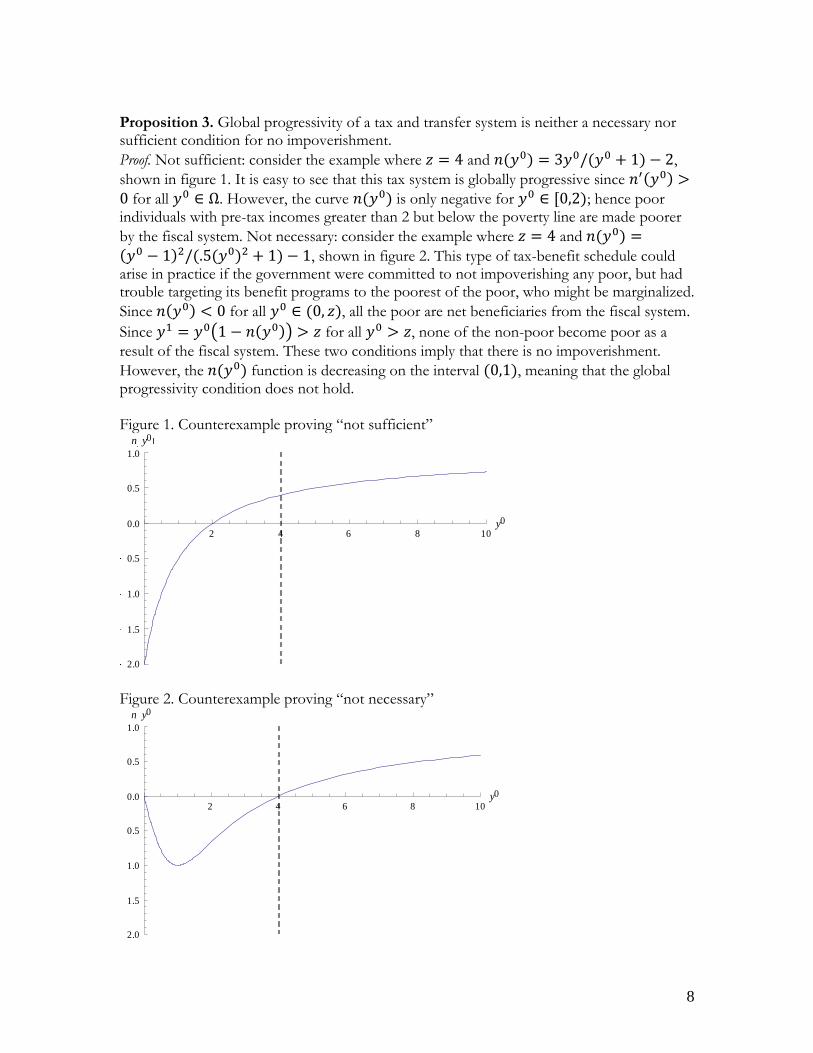
Proposition 3. Global progressivity of a tax and transfer system is neither a necessary nor sufficient condition for no impoverishment.

Proof. Not sufficient: consider the example where 𝑧 = 4 and 𝑛(𝑦0) = 3𝑦0/(𝑦0 + 1) − 2,

shown in figure 1. It is easy to see that this tax system is globally progressive since 𝑛′(𝑦0) >0 for all 𝑦0 ∈ Ω. However, the curve 𝑛(𝑦0) is only negative for 𝑦0 ∈ [0,2); hence poor individuals with pre-tax incomes greater than 2 but below the poverty line are made poorer

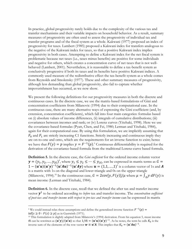
by the fiscal system. Not necessary: consider the example where 𝑧 = 4 and 𝑛(𝑦0) =(𝑦0 − 1)2/(.5(𝑦0)2 + 1) − 1, shown in figure 2. This type of tax-benefit schedule could arise in practice if the government were committed to not impoverishing any poor, but had trouble targeting its benefit programs to the poorest of the poor, who might be marginalized.

Since 𝑛(𝑦0) < 0 for all 𝑦0 ∈ (0, 𝑧), all the poor are net beneficiaries from the fiscal system.

Since 𝑦1 = 𝑦0(1 − 𝑛(𝑦0)) > 𝑧 for all 𝑦0 > 𝑧, none of the non-poor become poor as a

result of the fiscal system. These two conditions imply that there is no impoverishment.

However, the 𝑛(𝑦0) function is decreasing on the interval (0,1), meaning that the global progressivity condition does not hold. Figure 1. Counterexample proving “not sufficient”

Figure 2. Counterexample proving “not necessary”

2 4 6 8 10y0

2.0

1.5

1.0

0.5

0.0

0.5

1.0

n y0

2 4 6 8 10y0

2.0

1.5

1.0

0.5

0.0

0.5

1.0

n y0

9

In practice, global progressivity rarely holds due to the complexity of the various tax and transfer mechanisms and their variable impacts on household behavior. As a result, summary measures of progressivity are often used to assess the progressivity of individual tax and transfer programs and of the fiscal system as a whole. Kakwani (1977) proposed an index of progressivity for taxes. Lambert (1985) proposed a Kakwani index for transfers analogous to the negative of the Kakwani index for taxes, so that a positive Kakwani index implies progressivity in both cases. Attempting to define a Kakwani index for the net fiscal system is problematic because net taxes (i.e., taxes minus benefits) are positive for some individuals and negative for others, which creates a concentration curve of net taxes that is not well-behaved (Lambert, 2001). Nevertheless, it is reasonable to define a tax-benefit system as conclusively progressive if both its taxes and its benefits have positive Kakwani indices. A commonly used measure of the redistributive effect the tax-benefit system as a whole comes from Reynolds and Smolensky (1977). These and other summary measures of progressivity, although less demanding than global progressivity, also fail to capture whether impoverishment has occurred, as we now show. We present the following definitions for our progressivity measures in both the discrete and continuous cases. In the discrete case, we use the matrix-based formulations of Gini and concentration coefficients from Milanovic (1994) due to their computational ease. In the continuous case, there are many alternative ways of expressing the Gini coefficient (and, by extension, concentration coefficients), which fall into four main categories: formulas based on (i) absolute values of income differences, (ii) integrals of cumulative distributions; (iii) covariances between incomes and rank; or (iv) Lorenz curves (Yitzhaki, 1998). Here we use the covariance-based formulas (Pyatt, Chen, and Fei, 1980; Lerman and Yitzhaki, 1984), again for their computational ease. By using this formulation, we are implicitly assuming that

𝐹0 and 𝐹1 are strictly increasing C1 functions. Strictly increasing and continuous imply they are on-to-one and onto, which are the requirements for an inverse function to exist; hence

we have that 𝐹(𝑦) = 𝑝 implies 𝑦 = 𝐹−1(𝑝).9 Continuous differentiability is required for the derivation of the covariance-based formula from the traditional Lorenz-curve based formula. Definition 5. In the discrete case, the Gini coefficient for the ordered income column vector

𝒚 = (𝑦1, 𝑦2, … , 𝑦|𝑆|)′, where 𝑦1 ≤ 𝑦2 ≤ ⋯ ≤ 𝑦|𝑆|, can be expressed in matrix terms as 𝐺 =

1 − (𝒖′𝒖)(𝒖′𝒚)−1(𝒖′𝑨𝒖)−1(𝒖′𝑨𝒚) where 𝒖 = (1,1, … ,1)′ is a column vector of 1s and 𝑨 is a matrix with 1s on the diagonal and lower triangle and 0s on the upper triangle

(Milanovic, 1994).10 In the continuous case, 𝐺 = 2cov[𝑦, 𝐹(𝑦)]/𝜇 where 𝜇 = ∫Ω

𝑦 𝑑𝐹(𝑦) is

mean income (Lerman and Yitzhaki, 1984). Definition 6. In the discrete case, recall that we defined the after tax and transfer income

vector 𝒚1 to be ordered according to before tax and transfer income. The concentration coefficient of post-tax and transfer income with respect to pre-tax and transfer income can be expressed in matrix

9 We could instead relax these assumptions and define the generalized inverse function 𝐹−1(𝑝) =inf𝑠 ≥ 0 ∶ 𝐹(𝑠) ≥ 𝑝 as in Gastwirth (1971). 10 This formulation is slightly adapted from Milanovic’s (1994) derivation. From his equation 5, mean income

can be rewritten as (𝒖′𝒚)/(𝒖′𝒖) so that 1/ = (𝒖′𝒖)(𝒖′𝒚)−1. As he notes, the term he calls 𝐾0 is the

inverse sum of the elements of the row vector 𝒘 ≡ 𝒖′𝑨. This implies that 𝐾0 = (𝒖′𝑨𝒖)−1.

10

terms as 𝐶1 = 1 − (𝒖′𝒖)(𝒖′𝒚𝟏)−1(𝒖′𝑨𝒖)−1(𝒖′𝑨𝒚𝟏) (Milanovic, 1994). In the continuous

case, 𝐶1 = 2cov[𝑦1, 𝐹(𝑦0)]/𝜇1 where 𝜇1 ≡ ∫Ω

𝑦1 𝑑𝐹1(𝑦) is mean income after taxes and

transfers (Kakwani, 1980; Jenkins, 1988).

Definition 7. Denote the taxes paid (benefits received) by individual 𝑖 as 𝑡𝑖 (𝑏𝑖). By

definition, 𝑦𝑖1 = 𝑦𝑖

0 − 𝑡𝑖 + 𝑏𝑖. In the discrete case, let 𝒕 = (𝑡1, 𝑡2, … , 𝑡|𝑆|)′ be the column

vector of taxes paid with mean 𝑡 and 𝒃 = (𝑏1, 𝑏2, … , 𝑏|𝑆|)′ be the column vector of benefits

received with mean , both ordered by pre-tax and transfer income 𝑦0. The concentration

coefficient of taxes is 𝐶𝑡 = 1 − (𝒖′𝒖)(𝒖′𝒕)−1(𝒖′𝑨𝒖)−1(𝒖′𝑨𝒕) (Milanovic, 1994) and, similarly,

the concentration coefficient of benefits is 𝐶𝑏 = 1 − (𝒖′𝒖)(𝒖′𝒃)−1(𝒖′𝑨𝒖)−1(𝒖′𝑨𝒃). In the continuous case, taxes and benefits can be thought of as (possibly stochastic) functions of

pre-tax and transfer income and other characteristics 𝑡(𝑦0,⋅) and 𝑏(𝑦0,⋅), with means 𝑡 =

∫Ω

𝑡(𝑦0,⋅) 𝑑𝐹0(𝑦) and = ∫Ω

𝑏(𝑦0,⋅) 𝑑𝐹0(𝑦). Then 𝐶𝑡 = 2cov[𝑡(𝑦0,⋅), 𝐹(𝑦0)]/𝑡 and

𝐶𝑏 = 2cov[𝑏(𝑦0,⋅), 𝐹(𝑦0)]/ (Kakwani, 1980; Jenkins, 1988). Definition 8. The Reynolds-Smolensky index of post-tax and transfer income with respect to pre-tax and

transfer income is 𝑅 ≡ 𝐺0 − 𝐶1 (Reynolds and Smolensky, 1977). The fiscal system is

summarized as progressive if 𝑅 > 0.

Definition 9. The Kakwani index of taxes is 𝐾𝑡 ≡ 𝐶𝑡 − 𝐺0 (Kakwani, 1977) and the Kakwani

index of transfers is 𝐾𝑏 ≡ 𝐺0 − 𝐶𝑏 (Lambert, 1985). Taxes are summarized as progressive if

𝐾𝑡 ∈ (0, 1 − 𝐺0] and benefits are summarized as progressive if 𝐾𝑏 ∈ (0, 1 + 𝐺0]. If taxes are summarized as progressive and benefits are summarized as progressive, we say that the net fiscal system is summarized as progressive. Proposition 4. A tax-benefit system being summarized as progressive by the Kakwani coefficients for taxes and transfers or the Reynolds-Smolensky index of redistributive effect is neither a necessary nor sufficient condition for no impoverishment.

Proof. Not sufficient: consider the example where 𝒚𝟎 = (5, 8, 20), 𝒚𝟏 = (9, 6, 14), 𝑧 = 10,

taxes are 𝒕 = (1, 4, 7) and benefits 𝒃 = (5, 2, 1). Since this a discrete example, we use the

Gini and concentration coefficient formulations from Milanovic (1994). We have 𝑅 =0.141, 𝐾𝑡 = 0.023, 𝐾𝑏 = 0.477, which indicate a progressive net fiscal system, but impoverishment has occurred. Not necessary: consider an example with no impoverishment

where 𝒚𝟎 = (8, 13, 20), 𝒚𝟏 = (8, 11, 22), 𝑧 = 10, 𝒕 = (1, 3, 1), 𝒃 = (1, 1, 3). Since this is a discrete example, we use the Gini and concentration coefficient formulations from

Milanovic (1994). We have 𝑅 = −0.024, 𝐾𝑡 = −0.146, 𝐾𝑏 = −0.054, indicating that the net fiscal system can be summarized as regressive. Having seen that impoverishment can occur despite stochastic dominance of the post-fisc over the pre-fisc distribution and progressive taxes and transfers, we turn to the question of whether there are sufficient conditions—using these measures—to determine that impoverishment has or has not occurred. Proposition 5 shows that if the post-tax and transfer distribution does not weakly first order stochastically dominate the pre-tax and transfer distribution over the relevant domain, there was impoverishment of at least one poor person or of some non-poor person into poverty. Thus, the absence of weak stochastic

11

dominance of the post-fisc distribution over the pre-fisc distribution is a sufficient condition to establish that impoverishment has occurred. In order to be sure that no impoverishment has occured, a sufficient condition is the simultaneous fulfillment of weak stochastic dominance of the post-tax and transfer distribution over the pre-tax and transfer distribution and no re-ranking over the domain from zero to the maximum poverty line. This is shown in proposition 6.

Proposition 5. If 𝐹1 does not weakly first order stochastically dominate 𝐹0 among the poor, then impoverishment has occurred.

Proof. 𝐹1 does not weakly first order stochastically dominate 𝐹0 among the poor implies that

there exists a ∈ [0, 𝑧] such that 𝐹1() > 𝐹0(). By the definition of cumulative

distribution functions, this implies that the proportion of individuals with 𝑦𝑖1 < is higher

than the proportion of individuals with 𝑦𝑖0 < . Since the total number of individuals is

identical in the pre-tax and post-tax distributions, this implies that there exists some

individual 𝑗 such that 𝑦𝑗0 > and 𝑦𝑗

1 < . Since ≤ 𝑧, this implies 𝑦𝑗1 < 𝑦𝑗

0 and 𝑦𝑗1 < 𝑧,

implying impoverishment has occurred.

Proposition 6. If there is no reranking among the poor and 𝐹1 first order stochastically

dominates 𝐹0 among the poor, then impoverishment has not occurred.

Proof. By contrapositive: impoverishment among the poor implies that 𝑦𝑖1 < 𝑦𝑖

0 and 𝑦𝑖1 < 𝑧

for some individual 𝑖. If there does not exist an individual 𝑗 with 𝑦𝑗0 < 𝑦𝑖

0 ≤ 𝑦𝑗1 then

𝐹1(𝑦𝑖1) > 𝐹0(𝑦𝑖

1) which implies 𝐹1 does not first order stochastic dominate 𝐹0 on the

interval [0, 𝑧]. If there does exist such an individual 𝑗, then re-ranking has occurred. In practice, reranking is bound to occur (Lambert, 2001). Thus, the sufficient condition for the absence of impoverishment in proposition 6 is not very useful in practice, and the results from propositions 1-4 become even more important.

3. Illustration with Brazilian Data In this section, we show that stochastic dominance tests would lead us to conclude that Brazil’s tax and transfer system is unambiguously favorable to the poor, while progressivity measures reveal a progressive tax and benefit system. In spite of these positive outcomes, the extent of impoverishment is significant.11 Following the methods and income definitions outlined in Lustig and Higgins (2013), we compare market income (before taxes and transfers) to post-fiscal income (after direct and indirect taxes, direct cash and food transfers, and indirect subsidies). Market income includes labor income (including fringe benefits, vacation pay, etc.), capital income (rents, profits, interest, and dividends), private transfers (alimony, remittances, etc.), income from contributory pensions,12 imputed rent for owner-occupied housing, and goods produced for

11 This analysis uses the Pesquisa de Orçamentos Familiares (Family Expenditure Survey; POF) 2008-2009. 12 As described in Lustig, Pessino, and Scott (forthcoming), there is no agreement in the literature on whether contributory social security pensions should be treated as market income (similar to income from personal savings) or as a government transfer. Higgins and Pereira (forthcoming) analyze the tax and transfer system

12

own consumption. Direct taxes include the individual income tax, payroll taxes, and property taxes. Indirect taxes include consumption taxes at the state and national level.13 Direct transfers include conditional cash transfers (CCTs) from Brazil’s flagship anti-poverty program Bolsa Família, non-contributory pensions for the elderly and disabled, public scholarships, unemployment benefits, special circumstances pensions, milk transfers from Programa de Aquisição de Alimentos (PAA), and other direct transfers. Indirect subsidies include energy subsidies for low-income households.

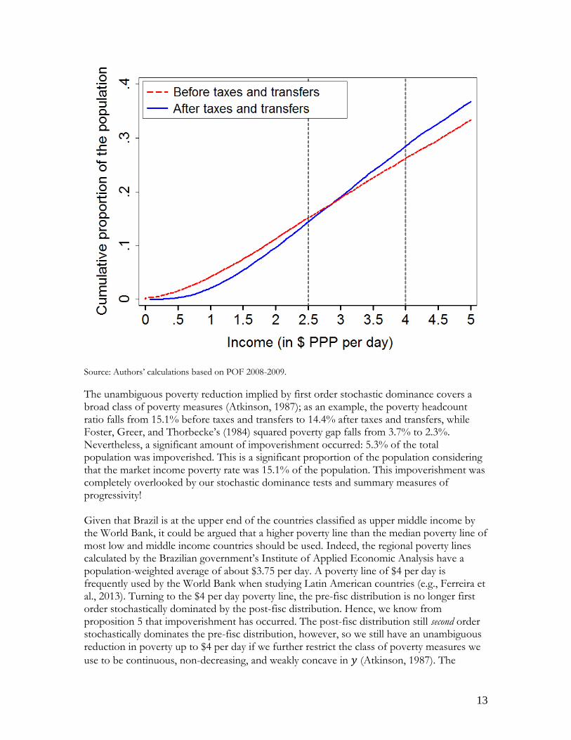
We begin by setting 𝑧 at $2.50 per day per household member, in 2005 US dollars adjusted for purchasing power parity (PPP). This line is equal to the median of the poverty lines calculated for the world’s low and middle income countries, excluding the fifteen poorest countries for which data is available (Chen and Ravallion, 2010). It is frequently the poverty line used to study the poor around the world (e.g., Banerjee and Duflo, 2007) and across Latin America (e.g., Levy and Schady, 2013). With a poverty line of $2.50 per day, poverty is unambiguously reduced by the fiscal system, as seen in figure 3. The after taxes and transfers income distribution first order stochastically dominates the before taxes and transfers income distribution for all poverty lines on the domain from $0 to $2.50. This dominance can be seen visually in figure 3; we verify that these dominance results are statistically significant using the asymptotic sampling distributions derived by Davidson and Duclos (2000) with a null hypothesis of non-dominance. Using a restricted domain that excludes the very lower tail for the reasons explained in Davidson and Duclos (2013) and goes up to the $2.50 per day income level, the null hypothesis is rejected at a 5% significance level. This dominance also implies, by Foster and Shorrocks (1988), that the welfare of the poor is increased for any (anonymous) monotonic utilitarian social welfare function that is additively separable.14 The fiscal system

can be summarized as progressive, as we have 𝑅 = 0.05, 𝐾𝑡 = 0.04, 𝐾𝑏 = 0.54. Figure 3. Cumulative distribution functions before and after taxes and transfers in Brazil

under both scenarios; for brevity, the illustration in this paper makes a choice between the two options, treating contributory pensions as market income, similar to private retirement income. 13 The consumption taxes included are the state-level Imposto sobre Circulação de Mercadorias e Serviços (ICMS) and the federal-level Imposto sobre Productos Industrializados (IPI). Our measures of post-fiscal income poverty and inequality differ from those in Higgins and Pereira (forthcoming) because that study includes two additional indirect taxes levied at the federal level: Programa de Integração Social (PIS) and Contribuição para o Financiamento da Seguridade Social (COFINS), relying on secondary source estimates of these taxes’ effective rates by decile. Because we do not include these federal indirect taxes in this illustration, our estimates of impoverishment and downward fiscal mobility in Brazil are likely to be lower bound estimates. 14 We include the condition of additive separability in order to meaningfully talk about the welfare of a particular sub-group of the population, namely the poor. Otherwise, this restriction would not be necessary. Saposnik (1981) shows that the ordering given by symmetric and monotonic social welfare functions is identical to the ordering given by symmetric, monotonic, and additively separable social welfare functions.

13

Source: Authors’ calculations based on POF 2008-2009.

The unambiguous poverty reduction implied by first order stochastic dominance covers a broad class of poverty measures (Atkinson, 1987); as an example, the poverty headcount ratio falls from 15.1% before taxes and transfers to 14.4% after taxes and transfers, while Foster, Greer, and Thorbecke’s (1984) squared poverty gap falls from 3.7% to 2.3%. Nevertheless, a significant amount of impoverishment occurred: 5.3% of the total population was impoverished. This is a significant proportion of the population considering that the market income poverty rate was 15.1% of the population. This impoverishment was completely overlooked by our stochastic dominance tests and summary measures of progressivity! Given that Brazil is at the upper end of the countries classified as upper middle income by the World Bank, it could be argued that a higher poverty line than the median poverty line of most low and middle income countries should be used. Indeed, the regional poverty lines calculated by the Brazilian government’s Institute of Applied Economic Analysis have a population-weighted average of about $3.75 per day. A poverty line of $4 per day is frequently used by the World Bank when studying Latin American countries (e.g., Ferreira et al., 2013). Turning to the $4 per day poverty line, the pre-fisc distribution is no longer first order stochastically dominated by the post-fisc distribution. Hence, we know from proposition 5 that impoverishment has occurred. The post-fisc distribution still second order stochastically dominates the pre-fisc distribution, however, so we still have an unambiguous reduction in poverty up to $4 per day if we further restrict the class of poverty measures we

use to be continuous, non-decreasing, and weakly concave in 𝑦 (Atkinson, 1987). The

14

second order dominance of the post-fisc distribution over the pre-fisc distribution can be

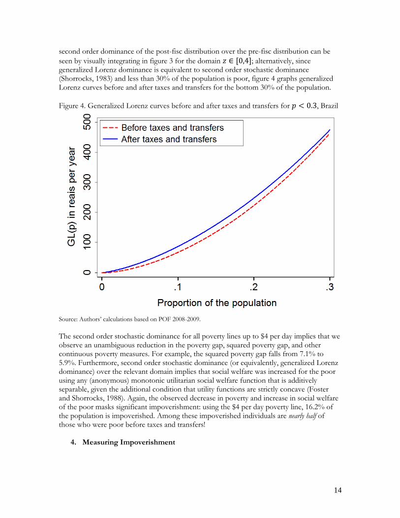
seen by visually integrating in figure 3 for the domain 𝑧 ∈ [0,4]; alternatively, since generalized Lorenz dominance is equivalent to second order stochastic dominance (Shorrocks, 1983) and less than 30% of the population is poor, figure 4 graphs generalized Lorenz curves before and after taxes and transfers for the bottom 30% of the population.

Figure 4. Generalized Lorenz curves before and after taxes and transfers for 𝑝 < 0.3, Brazil

Source: Authors’ calculations based on POF 2008-2009. The second order stochastic dominance for all poverty lines up to $4 per day implies that we observe an unambiguous reduction in the poverty gap, squared poverty gap, and other continuous poverty measures. For example, the squared poverty gap falls from 7.1% to 5.9%. Furthermore, second order stochastic dominance (or equivalently, generalized Lorenz dominance) over the relevant domain implies that social welfare was increased for the poor using any (anonymous) monotonic utilitarian social welfare function that is additively separable, given the additional condition that utility functions are strictly concave (Foster and Shorrocks, 1988). Again, the observed decrease in poverty and increase in social welfare of the poor masks significant impoverishment: using the $4 per day poverty line, 16.2% of the population is impoverished. Among these impoverished individuals are nearly half of those who were poor before taxes and transfers!

4. Measuring Impoverishment

15

Having seen both theoretically and empirically that our standard measures can overlook impoverishment, a natural starting point is to ask what the level of impoverishment is—in other words, what percent of the total population experiences impoverishment?15 Definition 10. The impoverishment headcount ratio simply measures the proportion of the population that are impoverished (i.e., that are either poor before taxes and transfers and made even poorer by the fiscal system, or non-poor before taxes and transfers and made

poor by the fiscal system). We have ℎ(𝒚𝟎, 𝒚𝟏) = |𝑆|−1 ∑ 𝕀(|𝑆|𝑖=1 𝑦𝑖

1 < 𝑦𝑖0)𝕀(𝑦𝑖

1 < 𝑧), where

𝕀(⋅) is the indicator function which has a value of 1 if its argument is true and 0 otherwise. As mentioned in section 3, for Brazil we have an impoverishment headcount ratio of 5.3% for the $2.50 per day poverty line and 16.2% at $4 per day. After determining the proportion of the population that is impoverished, the mobility literature provides a useful framework to further analyze impoverishment and convey this information to policymakers. We begin by defining a Markov transition matrix which, despite its shortcomings, provides information in a way that is easy to convey to policymakers. Transition matrices have been used to measure income mobility since Champernowne (1953); a thorough analysis of their use to measure mobility over time is provided by Shorrocks (1978). They were first used to measure mobility induced by the fiscal system in Atkinson (1980). Definition 11. A fiscal mobility matrix measures the directional movement between the before

and after net taxes situations among 𝑘 pre-defined income categories. It can be represented

by the 𝑘 × 𝑘 transition matrix 𝑃, where the 𝑖𝑗th element of 𝑃, denoted 𝑝𝑖𝑗, can be

interpreted as the probability of moving to income group 𝑗 after taxes and transfers for

individuals who were in income group 𝑖 before taxes and transfers. Hence, 𝑃 is a row

stochastic matrix with ∑ 𝑝𝑖𝑗𝑘𝑗=1 = 1 for all 𝑖 ∈ 1, … , 𝑘.

Define 𝒛 as a vector of poverty lines between 𝑧− and 𝑧+. In other words, 𝒛 = (𝑧−, … , 𝑧+) is an ordered vector whose component values define tranches of income ranges which

demarcate varying degrees of poverty severity.16 These poverty lines will determine a subset 𝑟

of the 𝑘 income categories (𝑟 < 𝑘) for which 𝑝𝑖𝑗 , 𝑗 ≤ 𝑟 and 𝑗 < 𝑖 denotes the probability of

moving into more severe poverty (poverty) after net taxes, for individuals who were less poor (not poor) before taxes and transfers.

Table 1 shows the fiscal mobility matrix 𝑃 for Brazil; the concatenated row (column) labeled “percent of population” give population shares for the market income (post-fiscal income) groups, while the last column gives the mean market income of members of that market

income group. We let 𝑘 = 4, 𝑟 = 2, 𝒛 = (2.5, 4), and the line separating the two non-poor groups is set at $10 PPP per day. The $10 per day line is the upper bound of those vulnerable to falling into poverty in three Latin American countries, calculated by Lopez-Calva and Ortiz-Juarez (2013). Ferreira et al. (2013) find that an income of around $10 per

15 Our methods of measuring impoverishment can be applied to two types of data: data in which actual taxes and benefits are enumerated, or data in which they are computed from a tax-benefit microsimulation model. 16 We are grateful to Peter Lambert for suggesting this interpretation of the vector of poverty lines.

16

day also represents the income at which individuals in various Latin American countries tend to self-identify as belonging to the middle class and use this as further justification that it should be used as the line to separate those vulnerable to falling into poverty from the middle class.17 We refer to the four groups as the extremely poor, moderately poor, vulnerable to poverty, and middle/upper class. Table 1. Fiscal Mobility Matrix for Brazil

Post-tax and transfer income groups

<2.5 2.5-4 4-10 >10 Percent of

population

Mean

income

Pre

-tax

an

d t

ran

sfer

inco

me

gro

up

s

<2.5 84.6% 10.4% 3.8% 1.2% 15.1% $1.45

2.5-4 13.9% 75.4% 10.1% 0.6% 11.1% $3.25

4-10 0.1% 12.6% 84.4% 2.8% 33.0% $6.68

>10 0.0% 0.0% 16.5% 83.5% 39.9% $28.85

Percent of

population

14.4% 14.1% 36.2% 35.8% 100.0% $14.57

Note: Mean incomes are measured in pre-tax income and are in US$ PPP per day. Rows may not sum to exactly 100% due to rounding. Differences in group shares between the before and after taxes and transfers distributions are all statistically significant from zero at the 0.1% significance level. Source: Authors’ calculations based on POF (2008-2009).

The fiscal mobility matrix tells us about impoverishment at a slightly more granular level and provides information that is easy to convey to policymakers. In the case of Brazil, we see that 13.9% of those who are moderately before taxes and transfers become extremely poor after taxes and transfers; 12.7% of those who are vulnerable to falling into poverty before taxes and transfers become poor after taxes and transfers. This impoverishment is mostly caused by indirect taxes; consumption tax exemptions are almost non-existent in Brazil (Corbacho, Cibils, and Lora 2013) and the multiple consumption taxes levied at the state and federal levels are high; hence the poor end up paying a large portion of their income in consumption taxes (Higgins and Pereira, forthcoming). The impoverishment headcount ratio measures the proportion who are impoverished but does not capture the amount that impoverished individuals lose, and the fiscal mobility matrix does not capture the impoverishment of poor individuals who remain in their income group. Hence, we also propose a measure of the dollar extent of impoverishment. Definition 12. The impoverishment gap measures the amount that would have to be transferred to the impoverished in order to eliminate impoverishment. It is measured in per capita terms (i.e., divided by the number of people in the population) in order to be population invariant.

Like the poverty gap, it could also be made homogenous of degree zero on Ω by normalizing

it by the poverty line. Here we use the non-normalized version. We have 𝑔(𝒚𝟎, 𝒚𝟏) =

|𝑆|−1 ∑ (min𝑦𝑖0, 𝑧 − min 𝑦𝑖

0, 𝑦𝑖1, 𝑧)

|𝑆|𝑖=1 .

17 The $10 PPP per day line was also used as the lower bound of the middle class in Latin America in Birdsall (2010) and in developing countries throughout the world in Kharas (2010).

17

Note that individuals who were poor before taxes and transfers and are impoverished (𝑦𝑖1 <

𝑦𝑖0 < 𝑧) contribute to the function 𝑔(⋅) by the amount they are impoverished, 𝑦𝑖

0 − 𝑦𝑖1.

Individuals who were non-poor before taxes and transers and are impoverished (𝑦𝑖1 <

𝑧 < 𝑦𝑖0) contribute to 𝑔(⋅) by the amount that would need to be transferred to them to get

them back to the poverty line (or equivalently, to prevent them from becoming

impoverished), 𝑧 − 𝑦𝑖1. Individuals who were not impoverished, either because they lost

income but remain above the poverty line or they did not lose income, contribute to 𝑔(⋅) by the amount 0.

For 𝑧 = 2.5, the impoverishment gap is just $0.01 per capita per day. This signifies that, if policy could be perfectly targeted to those who are impoverished, the elimination of impoverishment for this poverty line would not be particularly costly. However, the average

amount that an impoverished person is impoverished, given by 𝑔(𝒚𝟎, 𝒚𝟏)/ℎ(𝒚𝟎, 𝒚𝟏) = $0.19

per day, is significant considering their low incomes to be begin with. For 𝑧 = 4, the impoverishment gap is $0.05 per capita per day and the average amount an impoverished person is impoverished is $0.33 per day. A drawback of the impoverishment measures we have presented so far is that they may be

sensitive to the choice of 𝑧 (or 𝒛 in the case of the fiscal mobility matrix). If the chosen cut-offs represent discontinuities in the social cost of poverty (Bourguignon and Fields, 1997), this sensitivity is not as relevant. However, in the more likely scenario that the cut-offs are somewhat arbitrary, we can supplement our measures with graphical measures that overcome this limitation. We propose an impoverishment curve, and also make use of

Foster and Rothbaum’s (2013) downward mobility curve. For each possible poverty line 𝑧, the downward mobility curve simply measures the percent of the population that experienced downward mobility across that line; in other words, it is the proportion of the

population with 𝑦𝑖1 < 𝑧 < 𝑦𝑖

0. Definition 13. The downward mobility function from Foster and Rothbaum (2013) is

defined as 𝑚(𝑧,⋅) = |𝑆|−1∑𝑖=1|𝑆|

𝕀(𝑦𝑖0 > 𝑧)𝕀(𝑦𝑖

1 < 𝑧). Since we are concerned with

impoverishment, we will restrict it to being defined only on the domain 𝑧 ∈ [0, 𝑧+].

For a given poverty line , the downward mobility curve only captures the proportion of the

population that began above before taxes and transfers and was pushed below by taxes and transfers. This is only a subset of those who were impoverished, which includes those who

began below and were made even poorer by the tax-benefit system. In other words, if we

denote the set of individuals experiencing downward mobility across poverty line as 𝑄 =

𝑖 ∈ 𝑆 ∶ 𝑦𝑖1 < < 𝑦𝑖

0, the set of those who were poor before taxes and transfers and made

poorer by the fiscal system as 𝑃 = 𝑖 ∈ 𝑆 ∶ 𝑦𝑖1 < 𝑦𝑖

0 < , then 𝑄 ∩ 𝑃 = ∅ and the set of

impoverished 𝐼 = 𝑄 ∪ 𝑃. A useful function for the purposes of studying impoverishment is the impoverishment function, which measures the proportion of the population belonging

to the set 𝐼.

Definition 14. The impoverishment function is defined on the domain 𝑧 ∈ [0, 𝑧+] as

ℎ(𝑧,⋅) = |𝑆|−1 ∑ 𝕀(|𝑆|𝑖=1 𝑦𝑖

1 < 𝑦𝑖0)𝕀(𝑦𝑖

1 < 𝑧).

18

Given our discussion above, 𝑚(𝑧, 𝒚𝟏, 𝒚𝟐) ≤ ℎ(𝑧, 𝒚𝟏, 𝒚𝟐) for any 𝑧. These functions capture both the presence of impoverishment (like the impoverishment headcount ratio) and the amount lost (like the impoverishment gap). It is obvious that it captures the presence of impoverishment; to see that it captures the amount lost, consider an impoverished individual

𝑖 with 𝑦𝑖1 < 𝑦𝑖

0 < 𝑧+. Now consider an alternative scenario where the individual is

impoverished to a greater extent, and is left with income after taxes and transfers of 𝑖1

where 𝑖1 < 𝑦𝑖

1 < 𝑦𝑖0 < 𝑧+, while all other impoverished individuals 𝑗 ∈ 𝐼\𝑖 have 𝑗

1 =

𝑦𝑗1. The higher degree of impoverishment in the alternative scenario will not be overlooked

by the functions ℎ(𝑧,⋅) and 𝑚(𝑧,⋅): we have ℎ(𝑧, 𝟏,⋅) = ℎ(𝑧, 𝒚𝟏,⋅) + |𝑆|−1 for all 𝑧 ∈

(𝑖1, 𝑦𝑖

1) (i.e., for all poverty lines between 𝑖1 and 𝑦𝑖

1, downward mobility will be slightly

higher—by the amount |𝑆|−1—in the alternative scenario) while ℎ(𝑧, 𝟏,⋅) = ℎ(𝑧, 𝒚𝟏,⋅)

(i.e., the curves coincide) for all other 𝑧 in the domain. The same results obtain for the

function 𝑚(𝑧,⋅).

For a simple discrete example of this, suppose 𝑧+ = 4, 𝒚𝟎 = (1,2,3,5,10)′, 𝒚𝟏 =(3,1,2,5,10)′, 𝟏 = (3,1,1,6,10)′. In this example it is the third individual who has 𝑖

1 <

𝑦𝑖1 < 𝑦𝑖

0 < 𝑧+; specifically, 𝑖1 = 1, 𝑦𝑖

1 = 2, 𝑦𝑖0 = 3, 𝑧+ = 4. We have ℎ(𝑧, 𝟏,⋅) =

ℎ(𝑧, 𝒚𝟏,⋅) + 1/5 for 𝑧 ∈ (1,2) while ℎ(𝑧, 𝟏,⋅) = ℎ(𝑧, 𝒚𝟏,⋅) for all other 𝑧 in the domain.

Similarly, 𝑚(𝑧, 𝟏,⋅) = 𝑚(𝑧, 𝒚𝟏,⋅) + 1/5 for 𝑧 ∈ (1,2) while 𝑚(𝑧, 𝟏,⋅) = 𝑚(𝑧, 𝒚𝟏,⋅) for

all other 𝑧 in the domain. Figure 5 graphs the downward mobility and impoverishment curves in Brazil. It shows the

impoverishment headcount ratios we mentioned earlier for 𝑧 = 2.5 and 𝑧 = 4 of 5.3% and

16.2%, respectively, as well as the impoverishment headcount ratio for all other 𝑧 ∈ [0,4]. Using this information in combination with the downward mobility curve, we are able to see

at each what proportion of the impoverished belong to set 𝑄 = 𝑖 ∈ 𝑆 ∶ 𝑦𝑖1 < < 𝑦𝑖

0

and which to set 𝑃 = 𝑖 ∈ 𝑆 ∶ 𝑦𝑖1 < 𝑦𝑖

0 < . At the $4 per day poverty line, 4.2% of the population were non-poor before taxes and transfers but made poor by the fiscal system, while 12.1% of the population were poor before taxes and transfers and made poorer. The latter group makes up almost half of those who were poor before taxes and transfers. Figure 5. Downward mobility and impoverishment caused by the fiscal system, Brazil

19

Source: Authors’ calculations based on POF 2008-2009.

5. Impoverishment Dominance In order to compare impoverishment in two different post-fisc distributions with the same pre-fisc distribution (for example, when comparing the actual level of impoverishment to that which would occur after a policy reform), we propose partial downward mobility and impoverishment orderings involving first stochastic dominance tests of the downward mobility and impoverishment curves.18

Definition 15. Consider two alternative income distributions after taxes and transfers: 𝐹1𝐴

and 𝐹1𝐵, both generated from the same pre-tax and transfer income distribution 𝐹0. Situation

A first order downward mobility dominates (i.e., exhibits less downward mobility than) situation B

if 𝑚(𝑧, 𝒚𝑨𝟏 ,⋅) ≤ 𝑚(𝑧, 𝒚𝑩

𝟏 ,⋅) for all 𝑧 ∈ [0, 𝑧+] with strict inequality for at least one such 𝑧.

Situation A second order downward mobility dominates situation B if ∫ 𝑚(𝑐, 𝒚𝑨𝟏 ,⋅) 𝑑𝑐

𝑧

0≤

∫ 𝑚(𝑐, 𝒚𝑩𝟏 ,⋅) 𝑑𝑐

𝑧

0 for all 𝑧 ∈ [0, 𝑧+] with strict inequality for at least one such 𝑧.19

18 Comparing two post-fisc distributions with different pre-fisc distributions is more difficult because impoverishment and downward mobility are conditional on the pre-fisc distribution. Consider a comparison across two countries: a country with low pre-fisc poverty is likely to have lower impoverishment; a high density

of individuals above a particular ∈ [0, 𝑧+] in one country implies a higher probability of downward mobility

across in that country. Rothbaum (2012) proposes using the counterfactual reweighting techniques from Dinardo, Fortin, and Lemieux (1996) to overcome this issue. In this paper, we only consider comparisons that have the same pre-fisc distribution. 19 This definition is adapted from Foster and Rothbaum (2013).

20

Definition 16. Situation A first order impoverishment dominates (i.e., exhibits less impoverishment

than) situation B if ℎ(𝑧, 𝒚𝑨𝟏 ,⋅) ≤ ℎ(𝑧, 𝒚𝑩

𝟏 ,⋅) for all 𝑧 ∈ [0, 𝑧+] with strict inequality for at

least one such 𝑧. Situation A second order impoverishment dominates situation B if

∫ ℎ(𝑧, 𝒚𝑨𝟏 ,⋅) 𝑑𝑧

𝑐

0≤ ∫ ℎ(𝑐, 𝒚𝑩

𝟏 ,⋅) 𝑑𝑐𝑧

0 for all 𝑧 ∈ [0, 𝑧+] with strict inequality for at least one

such 𝑧. These dominance criteria can be used to determine when one situation has unambiguously less impoverishment (measured by either the headcount ratio or the impoverishment gap) than another. Specifically: Proposition 7. The impoverishment headcount ratio is unambiguously lower in situation A than

situation B for any poverty line 𝑧 in the domain [0, 𝑧+] if and only if situation A first order impoverishment dominates situation B. Proof. Trivial; follows immediately from the definition of first order impoverishment dominance. Proposition 8. The impoverishment gap is unambiguously lower in situation A than situation B

for any 𝑧 ∈ [0, 𝑧+] if and only if situation A second order downward mobility dominates situation B. Proof. See appendix. We illustrate by analyzing a recent state-level tax reform proposal in the United States: in early 2013, Louisiana governor Bobby Jindal proposed a revenue-neutral tax reform that would eliminate the state individual and corporate income taxes and generate increased revenue from the state sales tax by broadening its base and raising rates. We compare impoverishment under the actual fiscal system to that under the proposed reform.20 Impoverishment is unambiguously higher after the proposed reform. The market (before taxes and transfers) and post-fiscal (after taxes and transfers) income concepts are defined analogously to the case of Brazil. By the recommendation of the US Census Bureau’s Supplemental Poverty Measure (SPM) taskforce, both income concepts are net of medical out of pocket expenses and Medicare Part B premiums, work and childcare expenses, and child support paid (Short, 2012). Direct taxes include federal and state individual income taxes and state and local property taxes. We subtract direct taxes gross of any refundable tax credits, which we include separately as a direct transfer below. We do not include corporate income taxes due to the theoretical and empirical uncertainty surrounding its economic incidence (e.g., Auerbach, 2006). Indirect taxes include federal and state sales and excise taxes. Direct transfers include cash transfers, refundable tax credits, and near-cash or food transfers. Cash transfers include welfare programs,21 veteran’s benefits,

20 This comparison uses data from the 2010, 2011, and 2012 March Annual Social and Economic supplement of the Current Population Survey (CPS). We combine data from these three years because the CPS is only representative at the state level when using three-year averages. We use the integrated and harmonized version of the CPS data sets available from the University of Minnesota’s Integrated Public Use Microdata Series (IPUMS; King et al., 2013). 21 The questions on welfare programs includes federal and state-level welfare and welfare-to-work programs, Temporary Assistance for Needy Families (TANF), Aid to Families with Dependent Children (AFDC),

21

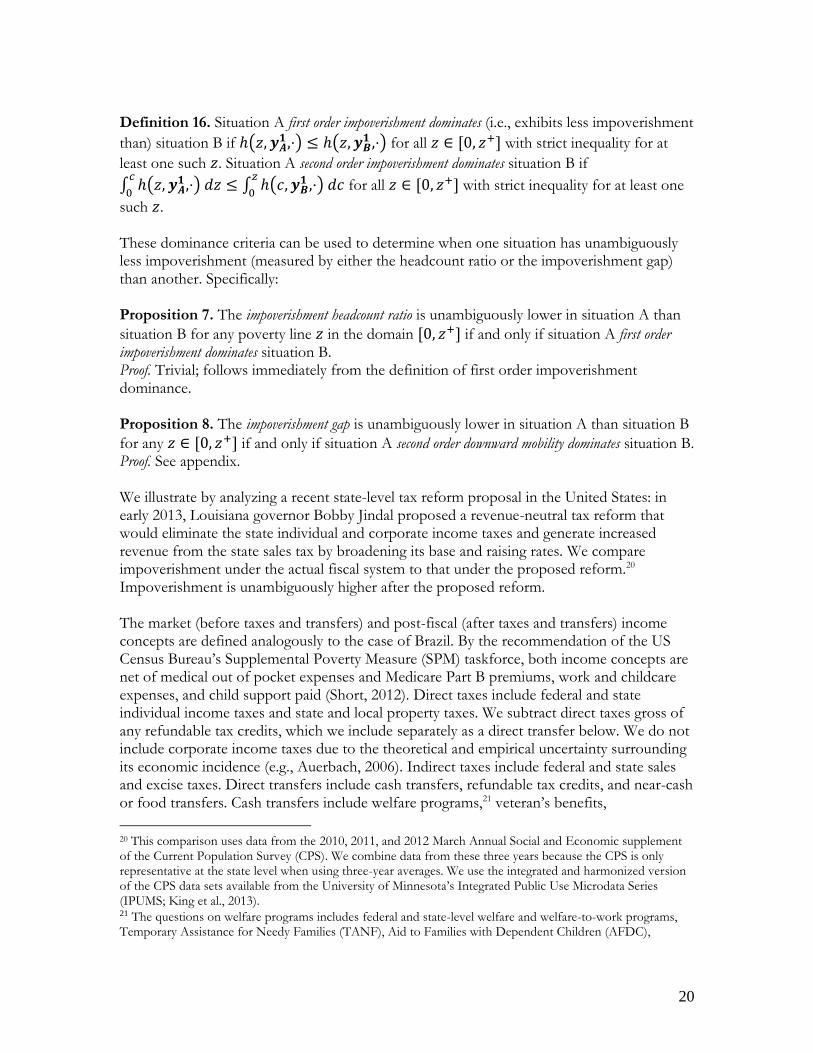
unemployment insurance, non-contributory pensions from the Supplemental Security Income program, and Pell Grants (a form of government scholarship). Refundable tax credits include federal and state earned income tax credits (EITC), federal child tax credits (CTC) and the making work pay (MWP) credit implemented as part of the American Recovery and Reinvestment Act of 2009. Near-cash benefits include those from the Supplemental Nutritional Assistance Program (SNAP, commonly known as “food stamps”), the Special Supplemental Nutrition Program for Women, Infants, and Children (WIC), and free and reduced-price school lunches for low-income families. Indirect subsidies include heating subsidies targeted to low-income households. To simulate Governor Jindal’s proposed tax reform, we eliminate all state income taxes. Because we do not include corporate income taxes in our analysis, we do not include this part of the reform; nevertheless, in 2012 corporate income taxes only made up 3% of Louisiana tax revenue, compared to 29% from individual income taxes (U.S. Census Bureau, 2013). Although it is unclear how the state EITC program would continue if the state income tax were eliminated, the governor (ambiguously) promised to include a similar program; hence, we do not eliminate the state EITC as part of our simulation. Because state EITC programs are well-targeted (Higgins et al., 2013), the decision of whether to eliminate them as part of the tax reform could potentially have an important impact on the incomes of poor households—and also on intergenerational mobility (see Chetty et al., 2013). Nevertheless, the state EITC in Louisiana is relatively small, providing the lowest benefits of all twenty-five states and three cities that have sub-federal EITC programs (Internal Revenue Service, 2013). Our dominance conclusions are robust to a sensitivity analysis where the program is eliminated. As originally proposed, the program was intended to be revenue neutral, with an increase in the state sales and excise tax rate intended to make up much of the lost revenue. Hence, we calculate the total amount of revenue collected by state income taxes in Louisiana and raise the amount each individual paid in state sales and excise taxes proportionally such that the same amount of total revenue is generated in the expanded survey data. We define poverty using the poverty lines calculated by the US Census Bureau’s SPM taskforce. These poverty lines vary by household type; on average, the poverty line equals $15.69 per household member per day in 2005 dollars. We divide total household income by the number of members of the household; we test the sensitivity of our results to instead using the equivalence scale calculated by SPM and the square root scale recommended by Atkinson, Rainwater, and Smeeding (1995) and find that our conclusions are robust to the choice of adjustment for economies of scale within households. Using our dominance criteria from section 4, impoverishment (as measured by either the impoverishment headcount or impoverishment gap) is unambiguously higher after the proposed tax reform. Figure 6 shows the impoverishment curve and the downward mobility curve under the actual fiscal system and Jindal’s proposed reform. Figure 6. Impoverishment dominance: higher impoverishment under proposed reform

Refugee Cash and Medical Assistance program, General Assistance/Emergency Assitance program, diversion payments, General Assistance from the Bureau of Indian Affairs, and Tribal Administered General Assistance.

22

Source: Authors’ calculations based on CPS 2010, 2011, 2012.

6. Social Welfare In section 3, we showed that first order stochastic dominance tests fail to capture impoverishment. We have argued throughout the paper that impoverishment is an important phenomenon that should be measured. How do we reconcile this argument with the traditional result that first order stochastic dominance implies higher social welfare for a broad class of social welfare functions? This traditional result uses anonymous social welfare functions: individual utilities and the social welfare function for the post-tax and transfer distribution are independent of what the pre-tax and transfer income distribution would have looked like, how much different individuals gained or lost from the tax-benefit system, and whether some of the individuals who lost were already unable to afford basic necessities. If individual utility functions or social welfare are dependent on the amount individuals gain or lose as well as their income level (as in Bourguignon, 2011), the traditional results no longer hold. Specifically, Bourguignon (2011) posits that individual utility is dependent on both post-

change income 𝑦𝑖1 and the amount gained or lost, 𝑥𝑖 = 𝑦𝑖

1 − 𝑦𝑖0. This contrasts with

standard social welfare measurement where utility depends only on income after taxes and

transfers 𝑦𝑖1. The “base” income 𝑦𝑖

0 in Bourguignon’s framework is usually status quo post-fisc income before some proposed reform to the fiscal system, against which post-fisc income under two potential reforms are compared. However, King (1983) posits that the ex

23

ante distribution could be taken to be the situation in the absence of taxes rather than the pre-reform ex post distribution, and Bourguignon (2011, p. 609) also mentions his framework’s applicability to a planner comparing two distributions on their distance from the market income distribution. Given such a utility function and the standard utilitarian social welfare criterion, social welfare in the actual tax and transfer system can be compared to that of the tax and transfer system in an alternative scenario or under a proposed reform.

He defines the surface 𝑍𝑋(𝑝, 𝑞), the mean income change for the 𝑞 ∈ [0,1] most

impoverished (or least enriched) proportion of the 𝑝 ∈ [0,1] poorest proportion of

individuals before taxes and transfers, in scenario 𝑋 ∈ 𝐴, 𝐵. Social welfare is higher under

tax and transfer system A than under system B if 𝑍𝐴(𝑝, 𝑞) ≥ 𝑍𝐵(𝑝, 𝑞) for all (𝑝, 𝑞) ∈[0,1] × [0,1] with strict inequality for at least one (𝑝, 𝑞) pair (Bourguignon, 2011). In the case of the proposed tax reform in Louisiana, we can thus compare social welfare in the actual scenario—dependent both on post-fisc income and the amount of income gained or lost with respect to the pre-fisc counterfactual—to that under the proposed reform.

When considering the social welfare of the entire population, the 𝑍𝑋(𝑝, 𝑞) functions cross; hence, neither scenario welfare dominates the other. This is not surprising, as we are considering a very broad class of social welfare functions that allow utility to be only weakly concave; some individuals (those that pay a comparatively large share of their income in state income taxes) stand to gain from the reform, while we have already seen that the impoverished stand to lose. Restricting our attention to those whose before tax and transfer income is less than two times the SPM poverty line (the poor and “near-poor” in the terminology of Heggeness and Hokayem [2013]), we do find that situation A welfare dominates situation B.22 Hence, if

individual utilities are monotonic in both post-fisc income 𝑦𝑖1 and in income change caused

by taxes and transfers, 𝑥𝑖 = 𝑦𝑖1 − 𝑦𝑖

0, the social welfare of those who have low or moderate pre-fisc income—which can be thought of as those who are either poor before taxes and transfers or vulnerable to falling into poverty—is unambiguously higher in the actual

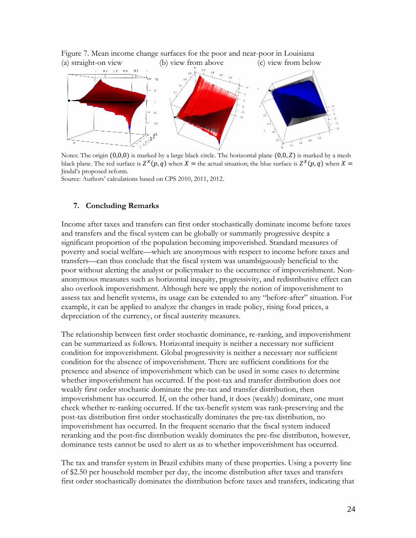
scenario than under the proposed reform. Figure 7 graphs the 𝑍𝑋(𝑝, 𝑞) surfaces for those who have pre-fisc income less than two times the poverty line, with the actual scenario in red and proposed reform in blue; as can be seen, the red surface is everywhere above the blue surface, from which it follows (Bourguignon, 2011) that the actual scenario welfare dominates the proposed reform.

22 This conclusion presumes that social welfare is additively separable, so that we can meaningfully talk of the social welfare of the sub-group with pre-fisc incomes below twice the poverty line. We restrict our attention to this group because no one with pre-fisc income above two times the poverty line is impoverished. The conclusion that the actual situation dominates the proposed reform is verified empirically but illustrated graphically.

24

Figure 7. Mean income change surfaces for the poor and near-poor in Louisiana (a) straight-on view (b) view from above (c) view from below

Notes: The origin (0,0,0) is marked by a large black circle. The horizontal plane (0,0, 𝑍) is marked by a mesh

black plane. The red surface is 𝑍𝑋(𝑝, 𝑞) when 𝑋 = the actual situation; the blue surface is 𝑍𝑋(𝑝, 𝑞) when 𝑋 = Jindal’s proposed reform. Source: Authors’ calculations based on CPS 2010, 2011, 2012.

7. Concluding Remarks Income after taxes and transfers can first order stochastically dominate income before taxes and transfers and the fiscal system can be globally or summarily progressive despite a significant proportion of the population becoming impoverished. Standard measures of poverty and social welfare—which are anonymous with respect to income before taxes and transfers—can thus conclude that the fiscal system was unambiguously beneficial to the poor without alerting the analyst or policymaker to the occurrence of impoverishment. Non-anonymous measures such as horizontal inequity, progressivity, and redistributive effect can also overlook impoverishment. Although here we apply the notion of impoverishment to assess tax and benefit systems, its usage can be extended to any “before-after” situation. For example, it can be applied to analyze the changes in trade policy, rising food prices, a depreciation of the currency, or fiscal austerity measures. The relationship between first order stochastic dominance, re-ranking, and impoverishment can be summarized as follows. Horizontal inequity is neither a necessary nor sufficient condition for impoverishment. Global progressivity is neither a necessary nor sufficient condition for the absence of impoverishment. There are sufficient conditions for the presence and absence of impoverishment which can be used in some cases to determine whether impoverishment has occurred. If the post-tax and transfer distribution does not weakly first order stochastic dominate the pre-tax and transfer distribution, then impoverishment has occurred. If, on the other hand, it does (weakly) dominate, one must check whether re-ranking occurred. If the tax-benefit system was rank-preserving and the post-tax distribution first order stochastically dominates the pre-tax distribution, no impoverishment has occurred. In the frequent scenario that the fiscal system induced reranking and the post-fisc distribution weakly dominates the pre-fisc distributon, however, dominance tests cannot be used to alert us as to whether impoverishment has occurred. The tax and transfer system in Brazil exhibits many of these properties. Using a poverty line of $2.50 per household member per day, the income distribution after taxes and transfers first order stochastically dominates the distribution before taxes and transfers, indicating that

25

the fiscal system has unambiguously reduced poverty for any poverty line between zero and $2.50 per day and for any poverty measure in a broad class of additively separable measures. This also indicates that, for monotonic social welfare functions that are anonymous with respect to pre-fisc income, social welfare was unambiguously increased by the tax and transfer system. The fiscal system is also progressive using standard measures of progressivity and redistributive effect. However, these conclusions mask the fact that a significant portion of the population—5.3% (which is high considering that poverty before taxes and transfers at the $2.50 line is 15.1%)—is impoverished. In other words, they either begin poor and are made poorer by the tax and transfer system, or begin non-poor but are made poor by the tax and transfer system. We propose a number of impoverishment measures. The impoverishment headcount ratio measures the proportion of the population that is impoverished, while the impoverishment gap measures the per capita amount that would be needed to eliminate impoverishment if perfect targeting were possible. The fiscal mobility matrix is a useful tool for conveying information about impoverishment to policymakers; in the case of Brazil it showed us that 13.9% of the moderately poor were made extremely poor by the fiscal system, while 12.7% of those vulnerable to poverty were made poor. To overcome the sensitivity of these measures to the choice of cut-offs, we propose an impoverishment headcount curve and downward mobility curve. These curves naturally extend to dominance criteria that can be used to compare two post-fisc situations and determine whether one exhibits unambiguously more impoverishment. We illustrate these dominance criteria by comparing the actual fiscal system in the state of Louisiana to a proposed reform which would eliminate the state income tax and increase state sales taxes. Impoverishment is unambiguously higher under the proposed reform. Finally, we reconcile our insistence on checking for the impoverishment caused by a fiscal system with the well-known results that first order stochastic dominance is equivalent to welfare dominance for a broad range of social welfare functions. The utility functions used in these social welfare functions are anonymous with respect to pre-fisc incomes, whereas individuals’ actual utility may depend both on their post-fisc incomes and how much income they gained or lost at the hands of the fiscal system.

26

Appendix. Proof of proposition 8

For the poverty line 𝑧 = , partition the set 𝑆 into four subsets: 𝑃 = 𝑖 ∈ 𝑆 ∶ 𝑦𝑖1 < 𝑦𝑖

0 < ,

𝑄 = 𝑖 ∈ 𝑆 ∶ 𝑦𝑖1 < < 𝑦𝑖

0, 𝑅 = 𝑖 ∈ 𝑆 ∶ 𝑦𝑖0 < , 𝑦𝑖

0 ≤ 𝑦𝑖1, 𝑇 = 𝑖 ∈ 𝑆 ∶ 𝑦𝑖

0 > , 𝑦𝑖1 >

. For any set Γ ⊂ 𝑆, denote 𝑔Γ(𝑧,⋅) = |𝑆|−1 ∑ (min𝑦𝑖0, 𝑧 − min𝑦𝑖

0, 𝑦𝑖1, 𝑧)𝑖∈Γ and

𝑚Γ(𝑧,⋅) = |𝑆|−1 ∑ 𝕀(𝑦𝑖0 > 𝑧)𝕀(𝑦𝑖

1 < 𝑧)𝑖∈Γ .

Each 𝑖 ∈ 𝑃 experienced downward mobility on the interval [0, ] for all 𝑧 ∈ [𝑦𝑖1, 𝑦𝑖

0].

Hence, individual 𝑖 ∈ 𝑃 increased 𝑚𝑃(𝑧,⋅) by |𝑆|−1 for 𝑧 ∈ [𝑦𝑖1, 𝑦𝑖

0] and by 0 for 𝑧 < 𝑦𝑖1

and 𝑧 > 𝑦𝑖0. This implies that individual 𝑖 ∈ 𝑃 increased ∫ 𝑚𝑃(𝑐,⋅) 𝑑𝑐

0 by |𝑆|−1(𝑦𝑖

0 − 𝑦𝑖1);

summing over all 𝑖 ∈ 𝑃, ∫ 𝑚𝑃(𝑐,⋅) 𝑑𝑐

0= ∑ |𝑆|−1(𝑦𝑖

0 − 𝑦𝑖1)𝑖∈𝑃 . Since 𝑦𝑖

1 < 𝑦𝑖0 < ∀𝑖 ∈ 𝑃,

𝑔P(,⋅) = |𝑆|−1 ∑ (𝑦𝑖0 − 𝑦𝑖

1)𝑖∈𝑃 . This implies 𝑔P(,⋅) = ∫ 𝑚𝑃(𝑐,⋅) 𝑑𝑐

0 (i).

Each 𝑖 ∈ 𝑄 experienced downward mobility on the interval [0, ] for all 𝑧 ∈ [𝑦𝑖1, ], which

increases 𝑚𝑄(𝑧,⋅) by |𝑆|−1 for 𝑧 ∈ [𝑦𝑖1, ] and by 0 for all other 𝑧. Hence individual 𝑖 ∈ 𝑄

increased ∫ 𝑚𝑄(𝑐,⋅) 𝑑𝑐

0 by |𝑆|−1( − 𝑦𝑖

1); summing over all 𝑖 ∈ 𝑄, ∫ 𝑚𝑄(𝑐,⋅) 𝑑𝑐

0=

∑ |𝑆|−1( − 𝑦𝑖1)𝑖∈𝑄 . Since 𝑦𝑖

1 < < 𝑦𝑖0 ∀𝑖 ∈ 𝑄, 𝑔𝑄(,⋅) = |𝑆|−1 ∑ ( − 𝑦𝑖

1)𝑖∈𝑄 which

implies 𝑔Q(,⋅) = ∫ 𝑚𝑄(𝑐,⋅) 𝑑𝑐

0 (ii).

Each 𝑖 ∈ 𝑅 does not experience downward mobility on the interval [0, ]; summing over all

𝑖 ∈ 𝑅 and integrating over our domain, we have ∫ 𝑚𝑅(𝑐,⋅) 𝑑𝑐 = 0

0. Since 𝑦𝑖

0 < and 𝑦𝑖0 ≤

𝑦𝑖1 ∀ 𝑖 ∈ 𝑅, we have 𝑔R(,⋅) = |𝑆|−1 ∑ (𝑦𝑖

0 − 𝑦𝑖0)𝑖∈𝑅 = 0 = ∫ 𝑚𝑅(𝑐,⋅) 𝑑𝑐

0 (iii). Similarly,

each 𝑖 ∈ 𝑇 does not experience downward mobility, so ∫ 𝑚𝑇(𝑐,⋅) 𝑑𝑐 = 0

0. Since 𝑦𝑖

0 >

and 𝑦𝑖1 > ∀ 𝑖 ∈ 𝑇, 𝑔𝑇(,⋅) = |𝑆|−1 ∑ ( − )𝑖∈𝑇 = 0 = ∫ 𝑚𝑇(𝑐,⋅) 𝑑𝑐

0 (iv).

𝑆 = 𝑃 ∪ 𝑄 ∪ 𝑅 ∪ 𝑇 and 𝑃 ∩ 𝑄 ∩ 𝑅 ∩ 𝑇 = ∅ implies 𝑔(,⋅) = 𝑔𝑃(,⋅) + 𝑔𝑄(,⋅) + 𝑔𝑅(,⋅

) + 𝑔𝑇(,⋅) and 𝑚(𝑧,⋅) = 𝑚𝑃(𝑧,⋅) + 𝑚𝑄(𝑧,⋅) + 𝑚𝑅(𝑧,⋅) + 𝑚𝑇(𝑧,⋅) by their definitions.

Hence, by (i)-(iv), 𝑔(,⋅) = ∫ 𝑚(𝑐,⋅) 𝑑𝑐

0. This holds for all ∈ [0, 𝑧+] since the choice of

was arbitrary, which completes the proof. References Atkinson, A.B., 1980. Horizontal equity and the distribution of the tax burden, in: Aaron,

H.J., Boskins, M.J. (Eds.), The Economics of Taxation. Brookings, Washington DC. Atkinson, A.B., 1987. On the measurement of poverty. Econometrica 55, 749-764. Atkinson, Anthony B., Lee Rainwater, and Timothy M. Smeeding. 1995. Income distribution

in OECD countries: Evidence from the Luxembourg Income Study (LIS). Social

Policy Studies No. 18. Paris: Organization for Economic Cooperation and

Development.

27

Auerbach, Alan and Kevin Hassett. 2002. A new measure of horizontal equity. American Economic Review 92(4): 1116-1125.

Auerbach, Alan J. 2006. “Who Bears the Corporate Tax? A Review of What We Know.” In

James M. Poterba, ed., Tax Policy and the Economy, Volume 20. Cambridge, Mass.:

MIT Press.

Banerjee, Abhijit, and Esther Duflo. 2007. The economic lives of the poor. Journal of Economic Perspectives 21(1): 141-167.

Bibi, Sami and Jean-Yves Duclos. 2007. Equity and policy effectiveness with imperfect targeting. Journal of Development Economics 83: 109-140.

Birdsall, Nancy. 2010. “The (Indispensable) Middle Class in Developing Countries; or, The Rich and the Rest, Not the Poor and the Rest.” In Ravi Kanbur and Michael Spence, eds., Equity in a Globalizing World. Washington, D.C.: World Bank.

Bourguignon, F., 2011. Status quo in the welfare analysis of tax reforms. Review of Income and Wealth 57, 603-621.

Bourguignon, F., Fields, G. 1997. Discontinuous losses from poverty, generalized Pα measures, and optimal transfers to the poor. Journal of Public Economics 63, 155-175.

Champernowne, D.G., 1953. A model of income distribution. The Economic Journal 63, 318-351.

Chen, S., Ravallion, R. 2010. The developing world is poorer than we thought, but no less successful in the fight against poverty. Quarterly Journal of Economics 125(4): 1577-1625.

Chetty, Raj, Nathaniel Hendren, Patrick Kline, and Emmanuel Saez. 2013. The economic impacts of tax expenditures: evidence from spatial variation across the U.S. Working paper.

Clark, S., Hemming, R., Ulph, D., 1981. On indices for the measurement of poverty. The Economic Journal 91, 515-526.

Davidson, Russell and Jean-Yves Duclos. 2000. Statistical inference for stochastic dominance and for the measurement of poverty and inequality. Econometrica 68(6): 1435-1464.

Davidson, Russell and Jean-Yves Duclos. 2013. Testing for restricted stochastic dominance. Econometric Reviews 32(1): 84-125.

Dinardo, John, Nicole M. Fortin, and Thomas Lemieux. 1996. Labor market institutions and the distribution of wages, 1973-1992: a semiparametric approach. Econometrica 64(5): 1001-1044.

Duclos, J.-Y., 2008. Horizontal and vertical equity, in: Durlauf, S.N., Blume, L.E. (Eds.), The New Palgrave Dictionary of Economics, Second Edition. Palgrave Macmillan.

Duclos, J.-Y., Lambert, P. 2000. A normative and statistical approach to measuring classical horizontal inequity. Canadian Journal of Economics 33(1): 87-113.

Gastwirth, J.L. 1971. A general definition of the Lorenz curve. Econometrica 39, 1037-1039. Feldstein, M. 1976. On the theory of tax reform. Journal of Public Economics 6: 77-104. Ferreira, F.H.G., Messina, J., Rigolini, J., Lopez-Calva, L.F., Lugo, M.A., Vakis, R., 2013.

Economic Mobility and the Rise of the Latin American Middle Class. World Bank, Washington DC.

Fields, G.S. 2001. Distribution and Development. Cambrige: Russell Sage Foundation and MIT Press.

Fields, G.S., 2008. Income mobility, in: Durlauf, S.N., Blume, L.E. (Eds.), The New Palgrave Dictionary of Economics, Second Edition. Palgrave Macmillan.

28

Fields, G.S., Leary, J.B., Ok, E.A. 2002. Stochastic dominance in mobility analysis. Economics Letters 75: 333-339.

Foster, J., Greer, J., Thorbecke, E., 1984. A class of decomposable poverty measures. Econometrica 52, 761-766.

Foster, J., Rothbaum, J., 2013. Mobility curves: using cutoffs to measure absolute mobility. Working paper.

Foster, J., Shorrocks, A.F., 1988. Poverty orderings. Econometrica 56, 173-177. Heggeness, Misty and Charles Hokayem. 2013. Life on the edge: living near poverty in the

United States, 1966-2011. U.S. Census Bureau SEHSD Working Paper 2013-02. Higgins, S., Pereira, C. 2013. The effects of Brazil’s high taxation and social spending on the

distribution of household income. Public Finance Review, forthcoming. Higgins, S., Ruble, W., Lustig, N., Smeeding, T.M. 2013. Comparing Taxation, Transfers,

and Social Spending in Brazil and the United States. Working paper. Internal Revenue Service. 2013. States and local governments with earned income tax

credits. Accessed 28 Sep 2013. http://www.irs.gov/Individuals/States-and-Local-Governments-with-Earned-Income-Tax-Credit

Jenkins, S. 1988. Calculating income distribution indices from micro-data. National Tax Journal 41, 139-142.

Kahneman, D., Tversky, A., 1979. Prospect theory: an analysis of decision under risk. Econometrica 47, 263-292.

Kakwani, N.C., 1977. Measurement of tax progressivity: an international comparison. The Economic Journal 87, 71-80.

Kakwani, N.C. 1980. Income Inequality and Poverty: Methods of Estimation and Policy Applications.

Kharas, H., 2010. The emerging middle class in developing countries. Working Paper, OECD.

King, Mervyn A. 1983. “An Index of Inequality: With Applications to Horizontal Equity and Social Mobility.” Econometrica 51(1): 99-115.

King, M., Ruggles, S., Alexander, J.T., Flood, S., Genadek, K., Schroeder, M.B., Trampe, B., Vick, R. 2013. Integrated Public Use Microdata Serices, Current Population Survey. Minneapolis: University of Minnestoa. Accessed 23 Sep 2013. https://cps.ipums.org/cps/index.shtml

Lambert, P.J., 1985. On the redistributive effect of taxes and benefits. Scottish J. Poli. Econ. 32, 39-54.

Lambert, P.J., 2001. The Distribution and Redistribution of Income, Third Edition. Manchester University Press, Manchester.

Lerman, R., Yitzhaki, S. 1984. A note on the calculation and interpretation of the Gini index. Economic Letters 15, 363-368.

Levy, Santiago and Norbert Schady. Latin America’s social policy challenge: education, social insurance, redistribution. Journal of Economic Perspectives 27(2): 193-218.

Lopez-Calva, L.F., Ortiz-Juarez, E., 2013. A vulnerability approach to the definition of the middle class. Journal of Economic Inequality, forthcoming.

Lustig, N., Higgins, S., 2013. Commitment to equity assessment: estimating the incidence of social spending, subsidies and taxes handbook. Working Paper, Commitment to Equity.

Lustig, N., Pessino, C., Scott, J., 2013. The impact of taxes and social spending on inequality and poverty in Argentina, Bolivia, Brazil, Mexico, and Peru. Public Finance Review, forthcoming.

29

Milanovic, B. 1994. The Gini-type functions: an alternative derivation. Bulletin of Economic Research 46, 81-90.

Pyatt, G., Chen, C., Fei, J. 1980. The distribution of income by factor components. Quarterly Journal of Economics 95 (3), 451-473.

Reynolds, M., Smolensky, E., 1977. Public Expenditures, Taxes, and the Distribution of Income: The United States, 1950, 1961, 1970. Academic Press, New York.

Rothbaum, J. 2012. Income and Educational Mobility and Race in the United States. Ph.D. thesis, George Washington University.

Saposnik, Rubin. 1981. Rank-dominance in income distributions. Public Choice 36(1): 147-151.

Shorrocks, A.F., 1987. The measurement of mobility. Econometrica 46(5): 1013-1024. Shorrocks, A.F., 1983. Ranking income distributions. Economica 50, 3-17. Short, Kathleen. 2012. The research Supplemental Poverty Measure: 2011. U.S. Census

Bureau Report. http://www.census.gov/prod/2012pubs/p60-244.pdf

van de Ven, J., Creedy, J., Lambert, P. 2001. Close equals and calculation of the vertical, horizontal and reranking effects of taxation. Oxford Bulletin of Economics and Statistics 63(3): 381-394.

Watts, H.W., 1968. An economic definition of poverty, in: Moynihan, D.P. (Ed.), On Understanding Poverty: Perspectives from the Social Sciences. Basic Books, New York.

U.S. Census Bureau. 2013. Quarterly Summary of State & Local Tax Revenue. http://www.census.gov/govs/qtax/