University of Nebraska - Lincoln DigitalCommons@University of Nebraska - Lincoln NASA Publications Nationa l Aeronautics and Space Administration 1-5-1999 Measuring Fractional Cover and Leaf Area Index in Arid Ecosyst ems: Digital C amera, Radiation Transmiance, and Laser Altimetry Methods Michae l A. W hite University of Montana - Missoula Gregory P. Asner University of Colorado at Boulder Ramakrishna R. Nemani University of Montana - Missoula Je L. Privee NASA Goddar d Space Fligh t Center Steven W. Running University of Montana - Missoula is Article is brought to you for free and open access by the National Aeronautics and Space Administration at DigitalCommons@University of Nebraska - Lincoln. It has been accepted for inclusion in NASA Publications by an authorized administrator of DigitalCommons@U niversity of Nebraska - Lincoln. White, Michael A.; A sner, G regory P .; Nema ni, Ramakrishna R.; Privee , Je L.; an d Running, Steve n W ., "Measurin g Fractio nal Cover and Leaf Area Index in Arid Ecosystems: Digital Camera, Radiation Transmiance, and Laser Altimetry Methods" (1999). NASA Publicatio ns. Paper 23. hp://digitalcommons.unl.edu/nasapub/23

Welcome message from author
This document is posted to help you gain knowledge. Please leave a comment to let me know what you think about it! Share it to your friends and learn new things together.
Transcript

8/13/2019 Measuring Fractional Cover
http://slidepdf.com/reader/full/measuring-fractional-cover 1/14
University of Nebraska - Lincoln
DigitalCommons@University of Nebraska - Lincoln
NASA Publications National Aeronautics and Space Administration
1-5-1999
Measuring Fractional Cover and Leaf Area Index in Arid Ecosystems: Digital Camera, Radiation
Transmiance, and Laser Altimetry MethodsMichael A. W hiteUniversity of Montana - Missoula
Gregory P. AsnerUniversity of Colorado at Boulder
Ramakrishna R. NemaniUniversity of Montana - Missoula
Je L. Privee
NASA Goddard Space Flight Center
Steven W. Running University of Montana - Missoula
is Article is brought to you for free and open access by the National Aeronautics and Space Administration at DigitalCommons@University of
Nebraska - Lincoln. It has been accepted for inclusion in NASA Publications by an authorized administrator of DigitalCommons@University of
Nebraska - Lincoln.
White, Michael A.; Asner, Gregory P.; Nemani, Ramakrishna R.; Privee, Je L.; and Running, Steven W., "Measuring FractionalCover and Leaf Area Index in Arid Ecosystems: Digital Camera, Radiation Transmiance, and Laser Altimetry Methods" (1999).
NASA Publications. Paper 23.hp://digitalcommons.unl.edu/nasapub/23

8/13/2019 Measuring Fractional Cover
http://slidepdf.com/reader/full/measuring-fractional-cover 2/14
Measuring Fractional Cover and Leaf Area Indexin Arid Ecosystems: Digital Camera, RadiationTransmittance, and Laser Altimetry Methods
Michael A. White,* Gregory P. Asner,† Ramakrishna R. Nemani,* Jeff L. Privette,‡ and Steven W. Running*
F ield measurement of shrubland ecological properties is should be guided by consideration of the amount of timeand resources required to obtain measurements of the de- important for both site monitoring and validation of remote
sensing information. During the May 1997 NASA Earth sired variables. Our results suggest that the ADC is bothObserving System Jornada Prototype Validation Exercise, efficient and accurate for long-term or large-scale monitor-
we calculated plot-level plant area index, leaf area index, ing of arid ecosystems. ©Elsevier Science Inc., 2000 total fractional cover, and green fractional cover with data from four instruments: (1) a Dycam Agricultural DigitalCamera (ADC), (2) a LI-COR LAI-2000 plant canopy INTRODUCTIONanalyzer, (3) a Decagon sunfleck Ceptometer, and (4) a
Shrublands exist in hot, dry areas where high evaporativelaser altimeter. Estimates from the LAI-2000 and Cepto-demand greatly exceeds unpredictable and sparse precipi- meter were very similar (plant area index 0.3, leaf areatation (Evenari, 1985). Although estimates vary widely index 0.22, total fractional cover 0.19, green fractional(Townshend et al., 1991), pure shrublands cover approxi-cover 0.14), while the ADC produced values 5% to 10%mately 9% of the Earth’s vegetated surface (Waring andhigher. Laser altimeter values, depending on the heightRunning, 1998). Within the past century, many arid tocutoff used to establish total fractional cover, were either semiarid areas of the United States have experienced dra-higher or lower than the other instruments’ values: a 10-cmmatic shrub increases, usually at the expense of nativecutoff produced values ~80% higher, while a 20-cm cutoff grasses (Smith et al., 1997). While some shrub expansion produced values~30% lower.The LAI-2000 and Ceptometer may be related to persistent drought (Herbel et al., 1972),are designed to operate in homogenous canopies, not theevidence suggests that overgrazing and fire suppression sparse and irregular vegetation found at Jornada. Thus,are more important causes (Archer et al., 1995; Bryant et these instruments were primarily useful for relative within-al., 1990; Grover and Musick, 1990). Such conversions can site plant area index monitoring. Calculation of some pa-be detrimental to pastoral societies directly dependent onrameters required destructive sampling, a relatively slowgrassland extent and productivity. High shrub cover may and labor-intensive activity that limits spatial and temporal
also have beneficial effects, such as increasing runoff waterapplicability. Validation/monitoring campaigns thereforefor irrigation (Skarpe, 1990) or accelerating aquifer re-charge (Leduc et al., 1997). Thus, depending on local prior-ities, increased or decreased shrub populations may be* Numerical Terradynamic Simulation Group, School of Forestry,
University of Montana, Missoula, MO desired. Regardless of the goal, accurate monitoring of † Cooperative Institute for Research in Environmental Sciences, shrublandextent andvigor is important for natural resourceUniversity of Colorado, Boulder, CO
managers and for the people they serve.‡ NASA Goddard Space Flight Center, Code 923, Biospheric Sci-ences Branch Satellite remote sensing provides the only technically
Address correspondence to Michael A. White, NTSG/School of consistent and temporally regular means of monitoringForestry,Universityof Montana, Missoula,MT 59812, USA.E-mail: mike@
shrublands over large areas. In shrublands, remote sensingntsg.umt.eduReceived 12 June 1998; revised 5 January 1999. is hampered by a high proportion of bare soil, clump shad-
REMOTE SENS. ENVIRON. 74:45–57 (2000)
©Elsevier Science Inc., 2000 0034-4257/00/$–see front matter655 Avenue of the Americas, New York, NY 10010 PII S0034-4257(00)00119-X
This article is a U.S. government work, and is not subject to copyright in the United States.

8/13/2019 Measuring Fractional Cover
http://slidepdf.com/reader/full/measuring-fractional-cover 3/14
46 White et al.
owing effects, and nonlinear relationships between the established empirical corrections to calculate LAI fromrecorded PAI values (Chen, 1996; Deblonde et al., 1994;measured signal and the areal extent and leaf density of
shrubs (Huete et al., 1992). Since vegetation cover is always Fassnacht et al., 1994; Gower and Norman, 1991). Theconsensus from these and other studies is that while trans-low in shrublands, site variation in soil reflectance can lead
to unpredictable errors in the quantification of shrubland mittance methods can give consistent relative measure-
ments at a given site, quantitatively accurate measurementsecological properties (van Leeuwen and Huete, 1996).Therefore, field measurement of shrubland ecological require site-specific corrections factors. Digital cameras,to a lesser extent, have also been used to measure LAI.properties is often necessary to provide a context for the
interpretation and quantification of satellite data. Although For example, Law (1994) measured LAI in artificially con-structed shrub canopies, and Baker et al. (1996) measureda wide variety of shrubland parameters are useful in specific
applications, leaf area index (LAI) and fractional cover (F) LAI in Pseudotsuga menziesii trees.The Prototype Validation Exercise (PROVE) cam-are perhaps the most commonly used metrics.
LAI is the one-sided foliage area per ground area (m2 / paign, an activity of the NASA Earth Observing SystemAM-1 validation program, is one of a series of field researchm2). Stem area index (SAI, m2 /m2) is the one-sided stem
area per ground area, where “stem” includes dead leaves, projects designed to thoroughly, yet rapidly and economi-cally, characterize site surface and atmospheric conditions.branches, and stems. The sum of LAI and SAI is plant
area index (PAI, m2 /m2), the one-sided plant area per PROVE’s goal is to provide field context for and validationof airborne and satellite data in a consistent fashion overground area. In this paper, the terms PAI, LAI, and SAI
refer to mean plot-level values (including bare ground and a network of global validation test sites. To date, PROVEcampaigns have been conducted in desert shrubland and vegetation), while the terms shrub PAI, shrub LAI, and
shrub SAI refer to individual plants within the landscape. moist temperate ecosystems. We participated in the May 1997 PROVE campaign conducted at the Jornada Long-Total fractional cover (FT, dimensionless) is the areal pro-
portion of the landscape occupied by green or nongreen Term Ecological Research site (see Privette, this volume,for project description). Our primary goal was to estimate vegetation (PAI/shrub PAI). Green fractional cover (FG,
dimensionless) is the areal proportion of the landscape plot-level LAI, PAI, FG, and FT from in situ field data.Our secondary goal was to investigate a digital camera’soccupied by green vegetation (LAI/shrub LAI). In these
definitions of F, we assume that fractional cover within capability to measure ecologically relevant variables andto assess the camera’s field reliability and ease of use. Inshrub perimeters is 1.
LAI, PAI, FG, and FT are each important for different this paper, we conduct an intercomparison of results andrecommend the easiest and most reliable techniques forpurposes. Many climate and ecosystem models are strongly
influenced by LAI (Bonan, 1993; Chase et al., 1996) and future field research seeking to measure the same variablesin similar environments.thus rely on accurate estimates. LAI and PAI are critical
for research investigating the impacts of shrub populationson the partitioning of precipitation into runoff and evapo-
METHODStranspiration. Plot structural parameters, such as FT, areimportant in radiative transfer models (Be gue , 1993). FT Site Descriptionis also required for calculating satellite estimates of sensible TheJornada Long-Term Ecological Research site is locatedheat flux (Ricotta and Avena, 1997). Satellite remote sens- in the northern Chihuahuan desert northeast of Lasing can be used to estimate LAI (Asrar et al., 1984; Spanner Cruces, New Mexico, USA (32.5N, 106.8 W). Mean an-et al., 1990) and F (Duncan et al., 1993; Dymond et al., nual temperature is 16C and mean annual precipitation1992; Pickup et al., 1993) through correlations with the is 21 cm with 52% falling between July and Septembernormalized difference vegetation index (NDVI) or other (Schlesinger et al., 1990). In the late 19th century, grass
spectral indices. cover was extensive. Since then, shrub canopy cover hasConsequently, ground estimates of shrubland ecologi- increased while grass cover has decreased, possibly as thecal properties are important both for validation of remote result of fire suppression and grazing (Buffington and Her-sensing data and for long-term monitoring of site condi- bel, 1985; Schlesinger et al., 1990). The transitional sitetions. A wide variety of techniques are available for ob- where we conducted our research is centered around ataining these estimates. Instruments that measure radiation 26-m tower that was instrumented with meteorologicaltransmittance, including the LI-COR LAI-2000 Plant Can- sensors and a Cimel sunphotometer. The site is character-opy Analyzer (LI-COR Inc., Lincoln, NE, USA) and the ized by an open shrub canopy dominated by mesquiteDecagon sunfleck Ceptometer quantum line sensor (Deca- (Prosopis grandulosa), Mormon Tea (Ephedra aspera), andgon Devices, Inc., Pullman, WA, USA), may be used to Yucca (Yucca Glauca). Mesquite is by far the dominantcalculate PAI and/or shrub PAI. Ideally, transmittance in- species, comprising approximately 70% of the canopy struments would measure LAI, the more ecologically rele- cover, with Ephedra (20%) and Yucca (10%) making up
vant variable, but it is often difficult to separate green smaller portions of the landscape. Forb and grass species
exist in small numbers.leaf from nongreen leaf vegetation. Many researchers have

8/13/2019 Measuring Fractional Cover
http://slidepdf.com/reader/full/measuring-fractional-cover 4/14
Measuring Fractional Cover and LAI 47
Sampling between 0.75 lm and 1.05 lm. A Wratten 29 red filter isused to block radiation below 0.6 lm. The full CCD has We sampled the Jornada transitional site on May 22 toan angular field-of-view of 31.524.25. At a distance of May 24, 1997 with the five following approaches: (1) digital1 m, this equals an image size of 565429 mm. Idealimagery with an Agricultural Digital Camera (ADC), (2)conditions for ADC operation are constant radiation envi-radiation transmittance with an LAI-2000 Plant Canopy
ronments with view zenith angles close to 0. Since imagesAnalyzer, (3) radiation transmittance with a Ceptometer taken from nadir with a solar zenith angle less than one-quantum line sensor, (4) ecosystem height variation with
half the field of view in the larger ADC dimension canairborne laser altimetry, and (5) destructive sampling withproduce hot spot effects, operation should be conductedan LI-3000 leaf area meter and photographic analysis. We
with solar zenith angles of at least 15.sampled with the instruments as follows: the ADC, LAI-For ground transect sampling, the ADC was mounted2000, and Ceptometer at 5-m intervals along 100-m tran-
on a horizontal pipe attached to a ladder so that the ADCsects extending east, south, and west from the central was 280 cm above the ground. Image area at this heighttower; the LAI-2000 at individual component shrubs within was 160120 cm. We used a portable computer to releasethe landscape; the ADC from a cherry picker 25 m abovethe shutter. We moved the apparatus to each 5-m intervalthe surface; laser altimetry along four aerial transects atand completed each transect in about 20–25 minutes underthe tower site; and destructive sampling of single shrubsbright, sunny conditions between 12:30 p.m. and 3:00 p.m.representative of the dominant species. In the next sec-on May 23 (solar zenith angles between 15 and 29).
tions, we describe the use of each instrument and its range Additionally, we imaged the site from a cherry picker posi-of application in our study.tioned roughly 20 m southwest of the tower on May 22 atTo avoid future confusion, we first present a descrip-1:00 p.m. under bright, sunny conditions. We took 10 im-tion of our variable naming convention. This paper containsages in a circular pattern around the cherry picker basketan inevitably large number of variables; a complete variableat a height of 25 m (from approximately nadir angles),list is presented in Appendix A. In general, the naming
yielding images with a 1411-m ground resolution.convention is as follows. When preceded by “shrub,” vari- While it was possible to calculate continuous vegeta-ables refer to measurements made on individual shrubs;
tion indices with the ADC, NIR saturation in vegetatedif not, variables refer to mean values from the transects orpixels reduced the dynamic range of this approach. Thus,from the cherry picker. Subscripts are used to identify a binary variable such as bright vs. dark was preferable tothe instrument: “2000” for the LAI-2000; “cept” for thea continuous measure. FG was easily extracted from theCeptometer; “ADC” for the Agricultural Digital Camera;ADC and met this criterion.“laser” for laser altimetry; and “dest” for destructive sam-
To calculate FGADC, we used the soil segmentationpling. In cases where one instrument was used for multipleutility (Steve Heinold, Dycam Inc., Chatsworth, CA, USA).purposes, superscripts are used to specify what was mea-The program is a supervised classification. For each image,
sured: “dest” refers to measurements of the destructively the user selects a training area of bare soil from which the
sampled shrubs; “component” refers to measurements of soil segmentation utility calculates a soil ratio as the ratio
component shrubs throughout the landscape; and “mean”of R to NIR brightness. Since bare soil usually has R
refers to species-weighted mean values compiled frombrightness only slightly less than NIR brightness, the soil
component shrub data. Thus, PAIcomponent2000 is an LAI-2000
ratio is less than one, typically between 0.6 and 0.9 forplant area index measurement of a component shrub and
Jornada soils. A threshold value is set as 99.5% of the soilPAIdest
cept is a Ceptometer plant area measurement of a de-ratio. Green vegetation, characterized by low R and high
structively sampled shrub.NIR brightness, will have an R:NIR ratio less than that of bare soil. The soil segmentation utility estimates FG as the
Agricultural Digital Camera
percent of vegetated pixels below the 99.5% threshold. If We calculated FG from the ratio of red (R) to near-infrared the NIR response range had been greater, NIR values in(NIR) brightness as recorded in digital numbers by an otherwise saturated pixels would have been higher, leadingAgricultural Digital Camera (ADC, Dycam Inc., Chats- to lower R:NIR ratios. Vegetated pixels at saturation there-
worth, CA, USA). The ADC records images of dimension fore were not classified as soil. Use of FG, which is cali-496365 pixels using an 8.5-mm lens and an 8.5-mm focal brated internally for each image using the soil ratio, obvi-length. Brightness values are measured with a charge-cou- ates the absolute image calibration required for betweenpled device (CCD) consisting of a color filter array sensitive scene comparison of NDVI or other vegetation indices.to R and NIR wavelengths. The color filter array records Testing at Jornada showed that selection of differentradiation from 0.6 lm to 1.05 lm with 80% of the recorded bare soil areas within one image resulted in soil ratio values
value determined by radiation between 0.615 lm and 0.985 varying by up to 35%. If an aberrantly high soil ratio were lm (S. Heinold, Dycam Inc., personal communication). chosen, some bare soil would be classified as vegetation.Adjacent color filter array elements respond to different Alternatively, selection of a low soil ratio would cause some
vegetation to be classified as soil. To address this difficulty, wavelengths: R between 0.6 lm and 0.75 lm and NIR

8/13/2019 Measuring Fractional Cover
http://slidepdf.com/reader/full/measuring-fractional-cover 5/14
48 White et al.
Figure 1. Application of the soilsegmentation utility to ground
and cherry picker images. Leftpanels show a sample unproc-essed (top) and processed (bot-tom) ground transect image (280cm height, 160120-cm resolu-tion, FG0.77). Right panelsshow a sample unprocessed (top)and processed (bottom) cherry picker image (25 m height,1411-m resolution, FG0.14).Areas classified as soil appear asblack, while vegetated areas ap-pear as in the unprocessed image.
we calculated the image soil ratio as the mean of five We measured PAI2000 along the ground transects attwilight on May 23 under diffuse radiation conditions. Torectangular bare soil areas (approximately 5030 pixels) within each image, one from each corner and one from minimize the influence of canopy gaps and subsequent
PAI2000 underestimation (LI-COR, 1992), we used a 45the center. If most of the scene was vegetated, we stillused five soil ratio values, but were forced to shift the view cap. After one above-canopy measurement, we sam-
pled five intervals along the transect with the sensorlocation of individual samples within the scene. With thismethod, we calculated FGADC for: (1) individual ground pointed in the transect direction. We repeated this cycle
four times per transect with each transect requiring approx-images; (2) east, south, and west transects as the mean of the 20 component images per transect; (3) the plot as the imately 10 minutes. Besides yielding PAI2000, the data files
from the LAI-2000, when used with the C2000 analysismean of the three transects; and (4) individual and meancherry picker images. package (LI-COR, Lincoln, NE, USA), can also be used
to calculate the Beer’s law extinction coefficient (k) forFigure 1 shows an example of the soil segmentationmethod for ground and cherry picker images. The left each of the five view angles as the fraction of foliage per
unit LAI oriented toward the direction of incoming sky panels show an unprocessed (top) and processed (bottom)ground image mostly occupied by a single large shrub. radiation. For each transect, we calculated the mean PAI2000
from the 20 points per transect and plot-level PAI2000 asRight panels show the same sequence but for a cherry pickerimage including numerous shrubs. In the bottom panels, the mean of the three transects. We also sampled shrub
PAIcomponent2000 for Prosopis ( n45), Ephedra ( n2), and Yuccaareas classified as soil are black, while areas classified as
green retain the appearance of the unprocessed images. ( n3) under diffuse radiation conditions at dawn or twi-light. At each shrub, we took one above-canopy measure-ment and one measurement from each cardinal direction.LAI-2000
The LI-COR LAI-2000 (LI-COR, Lincoln, NE, USA) inte-Ceptometer grates radiation transmittance through the canopy at 0.32
lm to 0.49 lm at five different view zenith angles (0–7, The Ceptometer integrates instantaneous fluxes of photo-synthetically active radiation (PAR, 0.4–0.7 lm) along a16–28, 32–43, 47–58, and 61–74) to calculate PAI2000.
See Welles and Norman (1991) for a discussion of the wand consisting of 80 1-cm2 sensors. PAIcept may be calcu-lated based on methods described by Pierce and Runningtheoretical details.

8/13/2019 Measuring Fractional Cover
http://slidepdf.com/reader/full/measuring-fractional-cover 6/14
Measuring Fractional Cover and LAI 49
Table 1. Experimental Design
LAI 3000/stem Laser LAI-2000 Ceptometer ADC Photography Altimetry
Transects PAI PAI FG – –Cherry picker – – FG – –
Aircraft transects – – – – FTComponent shrubs shrub PAI – – – –Destructive shrubs shrub PAI shrub PAI – shrub LAI –
shrub SAI
Component shrubs refer to individual shrubs sampled throughout the stand with the LAI-2000. Destructive shrubs refer to individual shrubs that were sampled first by the LAI-2000 and Ceptometer and then by destructive methods.
(1988) using the unitless ratio of below-canopy PAR (Q i) Laser Altimetry to above-canopy PAR (Qo), the extinction coefficient (k), Laser altimetry can be used to establish height variationand the Beer-Lambert law [see Eq. (1)]: along linear transects. FT is equal to the number of laser
return signals greater than a specified height divided by PAIcept1n(Q i / Qo)/ k (1)the total number of signals. The method is well established
We derived k in two ways. First, we used the k value from and is described elsewhere (Ritchie et al., 1992; Weltz etthe LAI-2000 7 ring, as calculated with the C2000 program. al., 1994). Using pulsed galium arside laser altimetry dataSecond, following Pierce and Running (1988) we estimated taken from small aircraft along four 300-m transects at thek by inverting Eq. (1) and using PAI2000 [see Eq. (2)]: transitional site, two east–west and two north–south, J.
Ritchie provided estimates of FT calculated from 10-cm,k1n(Q i / Qo)/PAI2000 (2)20-cm, 30-cm, and 40-cm height thresholds (personal com-
We measured Q i / Qo along the ground transects on May 22 munication). Each transect was composed of 16,384 indi- within 1 hour of solar noon in bright, sunny conditions. At vidual points with a 6-cm vertical precision. At 30-cm oreach point, we took one above-canopy measurement, two 40-cm cutoff, numerous small shrubs would have beenbelow-canopy measurements along the transect, two be- eliminated. Thus, we used both 10-cm and 20-cm cutoffslow-canopy measurements perpendicular to the transect, to calculate FTlaser.and a final above-canopy measurement. Each transect re-
quired approximately 15–20 minutes. We calculated mean Intercomparisontransect and mean plot PAIcept as for PAI2000. Table 1 shows a summary of input data. We directly mea-sured PAI, shrub PAI, shrub LAI, shrub SAI, and FG, and
Destructive Sampling we obtained estimates of FT from laser measurements. It We destructively measured LAIdest for one representative was then possible to estimate the full suite of variablesshrub each of Prosopis, Ephedra, and Yucca. To do so, we (PAI, LAI, FG, and FT) for each instrument (see Table 2manually harvested all green leaf material from the shrubs for equations). Initially, two intermediate variables had toand measured their one-sided LAIdest with a LI-COR LI- be calculated. First, the weighted ratio of total vegetation to3000 leaf area meter (LI-COR, Lincoln, NE, USA). We green vegetation (T:G) was calculated as shown in Eq. (3):calculated SAIdest from photographs of the woody materialremaining after leaf harvest. The sum of SAIdest and LAIdest
is equal to PAIdest. Prior to harvest, we measured shrub T:G
2
i0
w i shrub PAIdest i
2
i0 w i shrub LAIdest i
(3)
PAIdest
2000 and shrub PAIdest
cept for the three destructively sampledindividuals, once at dawn and once at dusk ( n8 for bothsets of measurements except for Yucca shrub PAIdest
cept where w i is the canopy percent dominance, assumed to be70% for Prosopis, 20% for Ephedra, and 10% for Yucca. where n6).
Table 2. Intercomparison Scheme
LAI-2000 andCeptometer ADC Laser Altimetry
PAI measured (2) FTshrub PAImean2000 (2) FTshrub PAImean
2000
LAI (1) PAI/T:G (3) PAI/T:G (3) PAI/T:GFT (2) PAI/shrub PAImean
2000 (1) FGT:G measuredFG (3) FT/T:G measured (1) FT/T:G
Variables were either measured or derived. Numbers represent order in which variables were calculated.

8/13/2019 Measuring Fractional Cover
http://slidepdf.com/reader/full/measuring-fractional-cover 7/14
50 White et al.
Table 3. Measured Variables
LAI-2000 Ceptometer Laser FT Laser FT Soil Ratio FG PAI PAI 10 cm 20 cm
East transect 0.77 (0.038) 0.13 (1.14) 0.27 (0.99) 0.23 (1.28) – – West transect 0.77 (0.030) 0.20 (1.18) 0.41 (1.09) 0.33 (1.60) – –
South transect 0.78 (0.023) 0.13 (1.20) 0.21 (1.06) 0.35 (1.21) – –All transectsa 0.77 (0.031) 0.15 (1.21) 0.30 (NA) 0.30 (1.40) 0.35 (0.062) 0.14 (0.065)Cherry picker 0.77 (0.017) 0.18 (0.27) – – – –
Soil ratio (red/near-infrared digital number); green fractional cover (FG); PAI from the LAI-2000 and Ceptometer; and total fractional cover fromlaser altimetry (FT). Values in parentheses are the coefficient of variation.
a For laser FT, all transects refers to the mean of four 300-m aircraft transects at the transitional site (two east–west, two north–south); for all other variables, all transects refers to the mean of the east, south, and west 100-m transects.
We assumed that T:G was constant for the entire transi- values used to calculate FGADC from both the transects andthe cherry picker were essentially identical. Difference of tional site.
Second, the species-weighted, mean shrub PAI over mean tests showed that soil ratios were not significantly different within ground transects, among ground transects,the entire plot was required for calculation of several pa-
rameters. Several alternatives existed. Mean shrub PAI within the cherry picker data, or between the ground and
cherry picker data. Ground transect soil ratio coefficientscould have been set to the species-weighted shrubPAIcomponent
2000 , but this would have assumed that using LAI- of variation (CVsstandard deviation/mean) were aroundtwice the cherry picker soil ratio CV. Since the images were2000 data in equations based on other instruments was
appropriate. In reality, this hybrid method might have not calibrated, we relied on the corrections for ambientradiation conditions inherent in individual image soil ratiotranslated errors created by unavoidable violation of LAI-
2000 assumptions (see below) to equations based on other calculations. Thus, despite the striking similarity in soilratios, the mean value could not be used to calculate FGADCinstruments. Mean shrub PAI could also have been calcu-
lated by assuming that shrub PAIdest was valid for the entire for all scenes.The ADC’s use of NIR information, as suggested by site. However, shrub PAIdest was based on only three data
points. Neither method was entirely satisfactory. Given the Law (1994) and implemented in the soil segmentation’scalculation of FGADC, allowed for easy discrimination be-available data, we adopted an alternative method capitaliz-
ing on the large number of individual shrub PAIcomponent2000 tween soil (larger R:NIR ratio) and vegetation (smaller
R:NIR ratio). Visual image analysis showed: (1) misclassifi- values and the physical rigor of the destructive measure-ments. We assumed that differences between shrub cation of dead vegetation as green material was minimal;(2) shadowed soil was correctly classified as soil; and (3)PAIdest
2000 and shrub PAIdest were caused by violation of LAI-2000 assumptions. We then calculated the ratio of shrub vegetation in deep shadow was classified as soil, leading
to a possible underestimation of FG. However, due toPAIdest2000 to shrub PAIdest (L:D). Both dawn and dusk shrub
PAIdest2000 data were used, resulting in two L:D values for limited self-shading in the sparse canopy and favorable
illumination angles, misclassification of vegetation as soileach species. We then corrected all shrub PAIcomponent2000 values
for each species using both L:D values and calculated the was also minimal. Mean FGADC was 0.15 for the groundtransects and 0.18 for the cherry picker (Table 3). Despitemean, species-weighted, shrub PAI: shrub PAImean
2000 .a factor of four difference in CVs between heights, FG ADC
was statistically indistinguishable between the cherry RESULTS AND DISCUSSION
picker and ground transects.At the Jornada site, the ADC, LAI-2000, Ceptometer, andlaser altimetry were used to produce estimates of PAI, Radiation Transmittance InstrumentsLAI, FT, and FG. However, no one instrument was univer- The ground transects’ PAI2000 and PAIcept were both 0.30sally well suited for measuring every parameter. In reality, (Table 3). In spite of the overall similarity, the ordinaleach instrument measured only one variable; the remain- relationships for the transects were not consistent: PAI2000
der were calculated with conversion factors, which were was highest in the west transect, while PAIcept was highestthemselves subject to uncertainties. In the following sec- in the south transect, near a transition to a more grassy tions, we present and discuss results for each instrument canopy. The range in PAI2000 was 0.2, while the range inand discuss the most appropriate tools for shrubland moni- PAIcept was only 0.12. Additionally, both instruments un-toring. avoidably violated major instrument assumptions.
The LAI-2000 assumes: (1) foliage is black (i.e., does ADC not transmit or reflect radiation); (2) foliage is randomly
distributed; (3) foliage elements are small in comparisonThe ADC produced consistent measurements of both the
soil ratio and FG. Table 3 shows that the ADC soil ratio to view areas; and (4) foliage is azimuthally randomly ori-

8/13/2019 Measuring Fractional Cover
http://slidepdf.com/reader/full/measuring-fractional-cover 8/14
Measuring Fractional Cover and LAI 51
Table 4. Calculation of the Total Vegetation to Green Vegetation Ratio (T:G)and the Mean Plot-Level Shrub Plant Area Index
Prosopis Ephedra Yucca Weighted glandulosa aspera glauca Meana
Shrub LAIdest 1.71 0.70 1.38 –
Shrub SAIdest 0.37 0.58 0.44 –Shrub PAIdest 2.08 1.28 1.82 –T:G 1.22 1.83 1.32 1.36L:D dawn 0.90 1.67 1.73 –L:D dusk 0.83 1.54 1.43 –Shrub PAIcomponent
2000 1.70 (0.33) 1.34 (0.014) 1.10 (0.51) –Shrub PAImean
2000 1.95 (0.38) 0.83 (0.040) 0.70 (0.30) 1.60 (0.27)
L:D is the ratio of shrub PAIdest2000 to shrub PAIdest, calculated from dawn and dusk PAI2000 data.
Shrub PAIcomponent2000 shows mean LAI-2000 measurements from individual component shrubs
throughout the plot. Shrub PAImean2000 is shrub PAIcomponent
2000 corrected for L:D. Data is parenthesesare one standard deviation.
a Weighted mean calculated with assumed 70% canopy cover for Prosopis, 20% for Ephedra,and 10% for Yucca.
ented. Yucca, with a regular distribution of large, planar, more samples than with the LAI-2000. Due to their uniquecanopy architecture, Yucca and Ephedra again representedstalklike leaves, violated the random foliage distribution
assumption. Effectively inserting the LAI-2000 wand un- the worst assumption violations.Ultimately, since both instruments produced similarder the Yucca foliage elements was difficult. Further, the
relatively massive size of the Yucca stalks violated the as- results, selection of one over the other may be guided by experimental conditions. The Ceptometer should be usedsumption that foliage elements are small compared to view in bright sunny conditions around solar noon, whereas theareas. Ephedra, containing photosynthetic stalks instead of LAI-2000 functions best under diffuse radiation conditionstrue leaves, has a clumped distribution that also violated(see Appendix B for discussion of instrument consistency the random foliage assumption. Prosopis, which is moreand optimal times of observation). If working in a sunny representative of broadleaf plants, did not seriously violateenvironment, such as Jornada, there will be approximately any assumptions.2 hours of useable time for the Ceptometer but only aboutThe L:D ratio provided a measure of the severity of
25–45 minutes for the LAI-2000 at dawn and dusk. Inthe LAI-2000’s violations. Not surprisingly, since Prosopis cloudy conditions, the LAI-2000 could be used throughouthad the least violation, its L:D was closest to unity. Boththe day. At Jornada, though, consistently low CVs (TableEphedra and Yucca had L:D values well above one. Viola-3) and an integrating transmittance-measuring techniquetion of random foliage distribution is routine in many appli-requiring fewer measurements at each point made thecations and in some cases does not seem to introduce largeLAI-2000 preferable to the Ceptometer.errors (Martens et al., 1993), while in other cases, especially
in highly clumped conifer vegetation, underestimation of Laser Altimetry PAI is common (Deblonde et al., 1994; Gower and Nor-
man, 1991; Stenberg et al., 1994). In our case, the L:D Laser altimetry data at the 10-cm cutoff produced highratios indicated that shrub LAI-2000 PAI should be cor- estimates, with FTlaser exceeding PAI2000 and PAIcept (Tablerected. 3). However, the assignment of FTlaser is entirely dependent
The Ceptometer was not an ideal instrument for Jorna- on the height cutoff used. By using the 10-cm cutoff, andda’s arid ecosystem. Major assumptions include: (1) spheri- especially considering the 6-cm vertical precision of thecal and random leaf inclination angle distribution, (2) ran- sensor, we were almost certain to include landscape ele-
ments unrelated to live or dead vegetation (Weltz et al.,dom foliage distribution, and (3) a homogeneous media.1994). At the 20-cm cutoff, most nonvegetation ground Vegetation aggregation in sparsely distributed clumps vio-elements and small forbs and grasses were probably ex-lated the Beer’s law assumption of a homogeneous media.cluded, leaving only fairly large shrubs. The ADC, on theThe Ceptometer’s major limitation was the requirementother hand, detected even very small foliage elements.of an independent estimate of the Beer’s law extinctionFTlaser was 0.35 with a 10-cm cutoff and 0.14 with a 20-cmcoefficient (k). Calculated from the LAI-2000 7 lens, kcutoff (Table 3). The CV was very low and very similar for was 0.35; from Eq. (2) using PAI2000 as an independent PAIboth height cutoffs.estimate, k was 0.36 (we used 0.35). Despite the consistent
results, calculation of k with either method was subject toDestructive Samplingthe LAI-2000’s assumptions, many of which were violated.
Additionally, because we were measuring point transmit- Up to now, we have considered the application and use of
the instruments in reference to the single variable they tance in a highly irregular canopy, we were forced to use
8/13/2019 Measuring Fractional Cover
http://slidepdf.com/reader/full/measuring-fractional-cover 9/14
52 White et al.
Figure 2. PAI, LAI, FG, and FG. LAI-2000 PlantCanopy Analyzer, Ceptometer quantum line sensor,and ADC data are the mean of three 100-m groundtransects. Laser altimetry data are the mean of four300-m aerial transects using 10-cm and 20-cmheight cutoffs.
actually measured. Calculation of the other variables relied and FG. Within variables, relationships were also consis-tent. Values based on the LAI-2000 or Ceptometer wereon conversion factors related to destructive sampling. We
assumed that the shrub LAIdest and shrub SAIdest values nearly identical. ADC-based data were slightly higher thanthe transmittance data, most likely because the ADC will were accurate. In reality, destructive sampling is notori-
ously difficult and inaccurate (e.g., Vertessy et al., 1995). detect low-lying grasses and forbs missed by both radiationtransmittance methods. Laser altimetry variables at the 10-For example, we were required to make subjective divisions
between green and nongreen portions of Yucca and Ephe- cm cutoff were by far the highest, nearly twice the LAI-2000 and Ceptometer variables. When the 20-cm cutoff dra vegetation. We further assumed that T:G and L:D,
although calculated from single shrubs, were applicable to was used, laser-based values were consistently the lowest.Indeed, Fig. 2 suggests that the laser results at the 20-cmthe entire plot. The shrubs selected for destructive sam-
pling and the T:G and L:D ratios calculated from these cutoff tended to exclude small vegetation elements but
that the 10-cm cutoff tended to include a large amount of shrubs may not have been representative of plot-level pat-terns. Shrub PAImean2000 , while based on LAI-2000 data, was nonvegetation material.
considered to be a surrogate for a larger destructive sample(planned for future campaigns). However, as shown by Shrubland Monitoring and ValidationChen (1996), even a very large destructive sample can still Based on this study, we suggest that routine monitoring
yield inaccurate results. of PAI, FG, and FT is practical in shrublands, especially Results from the destructive sampling and the calcula- within a single site. The ADC was ideally suited for measur-
tion of T:G and shrub PAImean2000 are presented in Table 4. ing shrubland FG, and at a cost of only about $1,000 was
Weighted T:G, primarily controlled by the Prosopis T:G relatively economical. The ADC was simple to operate andof 1.22, was 1.36. Component shrub sampling (shrub based on our experiences was very durable. While similarPAIcomponent
2000 ) showed highest values for Prosopis (1.70), fol- values were obtained from ground and cherry picker mea-lowed by Ephedra (1.34) and Yucca (1.10). Correction surements, ground transects are laborious and less efficientfor L:D slightly increased PAI for Prosopis (15%) and
than imagery from a greater height (see Appendix C forreduced PAI for Ephedra (38%) and Yucca (36). This discussion of scaling issues). We suggest that long-termindicates that violation of the random foliage assumption ADC monitoring in shrublands will be optimized by in Ephedra and Yucca in this system tended to produce mounting the ADC on a tower platform, such as the centralsignificantly inflated PAI measurements. Differences be- tower at the transitional site, and automating data gather-tween shrub PAImean
2000 and shrub PAIcomponent2000 for Prosopis were ing. This design, if built with a weather-proof camera (DY-
within the likely error of destructive sampling. Final shrub CAM, personal communication), would provide beneficialPAImean
2000 was 1.60. inclusion of several landscape elements in each image (asdescribed in Appendix C) and a temporally consistent
Intercomparison methodology independent of operator error. Alternatively, we suggest imaging from a helicopter, tower, or cherry Results from theintercomparison scheme outlined in Table
2 and calculated with the intermediate variables in Table 4 picker platform at a height 20 m above the surface. Withthe later approach, especially from helicopter, validationare shown in Fig. 2. The basic relationship between vari-
ables is immediately apparent. Regardless of the instru- of remote sensing estimates of FG should be possible andcomparable between numerous sites.ment, values were highest for PAI, followed by LAI, FT,

8/13/2019 Measuring Fractional Cover
http://slidepdf.com/reader/full/measuring-fractional-cover 10/14
Measuring Fractional Cover and LAI 53
Figure 3. Coefficient of variation for Prosopis,Ephedra, and Yucca shrub PAIdest
2000 and shrubPAIdest
cept from repeated measurements of one shrubper species. LAI-2000 data were taken under diffuseradiation conditions at dawn and dusk ( n8 for eachspecies at each time). Ceptometer data were takenunder bright sunlight ( n8 except for Yucca where n6).
FT was easily calculated from laser altimetry data and as the Jornada transitional site, only 30 to 40 observationsmay be required (as described in Appendix C). Relativethe 20-cm cutoff produced values generally comparable to
results from the ground-based instruments. For rapid FT PAI comparisons, both temporally and spatially, should bepossible with the LAI-2000.estimation over large areas where the cost of aircraft opera-
tion is not a factor, laser altimetry is an excellent option. Calculation of the full suite of variables from any oneinstrument or the calculation of LAI alone requires labori-For rapid and inexpensive PAI estimates, the LAI-2000
appeared to be the best option. In an environment such ous destructive sampling. Worse, the T:G and shrub
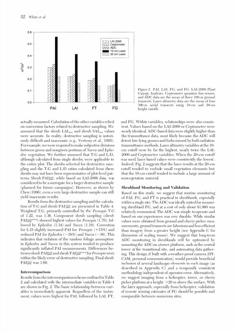
Figure 4. Bootstrap estimates of standard deviationfrom increasing sample size. (a) Ground-based LAIADC
and LAIcept standard deviations as sample size in-creased from 2 to 60. (b) LAIADC as estimated fromthe cherry picker as sample size increased from 2to 10.

8/13/2019 Measuring Fractional Cover
http://slidepdf.com/reader/full/measuring-fractional-cover 11/14
54 White et al.
PAImean2000 conversion factors, as pointed out by Dufre ˆ ne and evergreen forests with FG approaching 1.0. In deciduous
or open evergreen forests, the ADC could be used toBre da (1995), are not likely to be seasonally constant. Cer-tainly for the deciduous Prosopis, T:G will not be constant. monitor FG development, but obtaining a height great
enough to include multiple canopy elements would beThus, to rigorously monitor seasonal LAI, frequent de-structive sampling would be required. At a site such as expensive and experimentally difficult. For forest canopies,
we suggest one of two options for obtaining LAI. First, if Jornada, this would be too intrusive for future long-termstudies. Ideally, the ADC could be used to estimate LAI. measurements are required on a temporal scale of years,site-specific sapwood to leaf area allometric equations areHowever, the NIR saturation prevented us from account-
ing for even single scattering effects. If a more sensitive fairly accurate (e.g., Keane and Weetman, 1987; O’Haraand Valappil, 1995; Vertessy et al., 1995). Second, if suban-instrument were used in combination with species-specific
radiative transfer models, it would theoretically be possible nual data are required, transmittance instruments are thebest alternative. If quantitative data are needed, correctionto establish optimal view and illumination angles and to
establish correlations between destructively sampled LAI factors must be applied (Chen, 1996; White et al., 1997).If only relative changes within a plot are desired, the trans-and ADC brightness values. This method would provide:
(1) a one-time regression curve free of transmittance sen- mittance data may be used without correction. Despitehopes to the contrary, there is “no one size fits all” valida-sors’ need for repeated destruction, and (2) a viable means
of rapidly measuring LAI in the field. However, given tion or monitoring approach. Rather, variation in canopy structure mandates a biome-specific selection of both thecurrent liabilities, LAI will be difficult to monitor routinely.
The methodologies we have presented here provide most appropriate variable to measure and the measuringin-strument.a simple and rapid means of validating estimates of FG
throughout time and space and a somewhat more compli-cated means of validating LAI estimates at a single time We thank J. Ritchie for providing the laser altimetry results; C.
Wessman, S. Zunker, and M. Helmlinger for field assistance; andand place. For instruments operating at a relatively fine L. Rocchio for destructive sampling analysis. The JORNEX staff,spatial resolution, such as the Systeme Pour l’observationledby J. Lenz, provided andoperatedthe cherrypicker. S. Heinoldde la Terre (10 m) or the Thematic Mapper (30 m), opera- provided valuable technical assistance with the Agricultural Digi-
tion of the ADC as outlined here could easily provide tal Camera. Logistical support and equipment were providedcalibration of satellite fractional cover estimates at a large by the MODLAND project. M.A. White is supported by NASA
MODIS grant NAS5-31368 and the NASA ESS Fellowship Pro-number of sites relatively quickly. Validation of coarser gram. G. P. Asner is supported by NASA EOS IDS grant NAGW-resolution satellite data will be best accomplished from a 2662, NASA LCLUC grant NAG5-6134, and the NASA ESShelicopter platform. Appendix C suggests that a ModerateFellowship Program. R. R. Nemani and S. W. Running are sup-
Resolution Imaging Spectrometer 250-m pixel may be ade- ported by NASA MODIS grant NAS5-31368. J. L. Privette isquately characterized by nine observations, while an Ad- supported by NASA Headquarters RTOP 622-93-34.
vanced Very High Resolution Radiometer 1.1-km pixel willrequire about 150 observations. Moving to a height greaterthan the 25-m level used in this study should further reducethe required number of observations.
APPENDIX A: NOTATION LISTSUGGESTIONS FOR FUTURE WORK
In other short-canopy biomes, variation in canopy structureShrub Parameters
is likely to require a different combination of instrumentsShrub LAIdest LI-3000 leaf area index measurements of for ecological monitoring and satellite validation. For crop
the destructively sampled shrubs
canopies, typically with extremely small SAI, LAI can be Shrub SAIdest Photographic stem area indexdirectly measured with transmittance instruments (Hicks measurements of the destructively sampled shrubsand Lascano, 1995). Since even at peak growing season
Shrub PAIdest Calculated plant area index of thebiomass, grasslands can contain a large amount of deaddestructively sampled bushes vegetation mixed with green material (Singh and Gupta,
Shrub PAIdest2000 LAI-2000 plant area index measurements
1993), transmittance LAI estimates must be corrected forof the destructively sampled shrubs
T:G. In contrast to sparse shrub canopies, grassland T:G Shrub PAIdestcept Ceptometer plant area index measurements
of the destructively sampled shrubscould be repeatedly calculated without destroying the plot.Shrub PAIcomponent
2000 LAI-2000 plant area index measurementsThe ADC should be suitable for monitoring FG in bothof component shrubscrop and grassland canopies.
Shrub PAImean2000 Mean, species-weighted, corrected LAI-
While not specifically addressed in this paper, we spec-2000 plant area index measurements of
ulate that the greatly different canopy structure of forest component shrubsenvironments will necessitate different measurement strat-
(continued)egies. Use of the ADC will be inappropriate in closed

8/13/2019 Measuring Fractional Cover
http://slidepdf.com/reader/full/measuring-fractional-cover 12/14
Measuring Fractional Cover and LAI 55
Appendix A (Continued) zon is much farther away, resulting in a rapid transitionfrom sunlight to dark with a shorter period of diffuse radia-Plot-Level Parametersa
tion (~25 minutes). Based on these divergent radiationPAI2000 Plant area index measured with the LAI- conditions, it is likely that the dawn samples’ more consis-
2000tent radiation environment was manifested in lower CVs.
PAIcept Plant area index measured with the
CeptometerPAIADC Plant area index calculated from the
APPENDIX C: DEPENDENCE OF SAMPLEAgricultural Digital Camera
VARIABILITY ON SAMPLE SIZE ANDPAIlaser Plant area index calculated from laseraltimetry SPATIAL RESOLUTION
LAI2000 Leaf area index calculated from the LAI- We used a modified bootstrap analysis to assess the effects2000
LAIcept Leaf area index calculated from the of increasing sample size and spatial resolution on theCeptometer variability of mean plot-level estimates. The bootstrap
LAIADC Leaf area index calculated from the methodology for ground transects was as follows. First, weAgricultural Digital Camera
randomly selected two samples from the total pool of 60LAIlaser Leaf area index calculated from laserpoints (with replacement). We repeated this selection pro-altimetry
FT2000 Total fractional cover calculated from the cess for a total of 200 iterations. This produced a datasetLAI-2000 of 200 samples with n2. Second, we calculated the mean
FTcept Total fractional cover calculated from the of each of the 200 samples. Third, we calculated the stan-Ceptometer
dard deviation of the 200 means. Fourth, we repeated stepsFTADC Total fractional cover calculated from theone to three but with an increasing sample size until n60.Agricultural Digital Camera
FTlaser Total fractional cover measured with laser We completed the procedure for LAI, PAI, FT, and FG.altimetry For variables calculated with shrub PAImean
2000 (Table 2), weFG2000 Green fractional cover calculated from the used the normal approximation and randomly selected
LAI-2000shrub PAImean
2000 values for each of the 200 iterations. Unfortu-FGcept Green fractional cover calculated fromnately, since the point PAI2000 values were not retained, wethe Ceptometer
FGADC Green fractional cover measured with the were only able to use the bootstrap analysis for CeptometerAgricultural Digital Camera and ADC data.
FGlaser Green fractional cover calculated from Figure 4 shows the effect of increasing sample size onlaser altimetry
sample standard deviation. Results for FG, FT, PAI, and
Ratios LAI all showed the same pattern. We present ground datafor LAIADC and LAIcept in Fig. 4. Increasing sample size
T:G The ratio of shrub PAIdest to shrub LAIdest
from 2 to 12 resulted in a rapid decrease in standardL:D The ratio of shrub PAIdest2000 to shrub PAIdest
deviation followed by a slower decrease up to around 30.a “Measured” indicatesvariables immediately available frominstrumentIncreasing sample size past 30 produced only minor reduc-data. “Calculated” indicates variables calculated with the equations in
Table 2. tion in standard deviation. Figure 4b shows the same phe-nomenon for the cherry picker LAIADC. Here, no reductionin standard deviation was obtained past a sample size of APPENDIX B: VARIABILITY OF LAI-2000 ANDsix. Both the ground and cherry picker LAIADC standardCEPTOMETER DATA.deviations reached a minimum of around 0.6, but at the
Figure 3 shows the CVs for shrub PAIdest2000 and shrub ground resolution, approximately 30 images were required
PAIdestcept. CVs from the Ceptometer showed no clear relation- to approach the minimum. The cherry picker data, on the
ship with the LAI-2000 data, but were in the same general other hand, required only six images to reach the minimum.range. This suggests that within a single bush, neither Difference in ground resolution between the ground
instrument was inherently more consistent than the other. transects and the cherry picker revealed two patterns inFor all three species, the dawn shrub PAIdest
2000 had a lower the ADC data (Table 3). First, based on statistically indis-CV (less variable) than the dusk shrubPAIdest
2000. Prosopis tinguishable soil ratios and FGADC, the ADC is not sensitiveshowed the largest difference between dawn and dusk to variation in sensor height (to 25 m). Second, variability CVs. Differences in LAI-2000 wand placement might be in FGADC estimates appeared to be dependent on the rela-expected to cause some variation in CV, but not the consis- tionship between spatial resolution and landscape elementtently observed lower dawn CVs. We speculate that the size. Ground transect FGADC range was more than fourdifference between dawn and dusk LAI-2000 could have times larger than the cherry picker FGADC range (Table 3),been caused by differences in radiation environments. The and FGADC CVs were vastly larger than the cherry pickereast horizon at Jornada is formed by a nearby mountain CV. Evidently, a spatial resolution large enough to includerange. Thus, after sunrise, there is a fairly long period of multiple landscape elements resulted in more consistent
image to image FGADC estimates. Ground images couldconsistent diffuse radiation (~45 minutes). The west hori-

8/13/2019 Measuring Fractional Cover
http://slidepdf.com/reader/full/measuring-fractional-cover 13/14
56 White et al.
area index in conifer and broad-leaf plantations. Ecology 72:either contain large portions of shrubs or virtually no plant1896–1900.material, while cherry picker images always contained mul-
Grover, H. D., and Musick, H. B. (1990), Shrub land encroach-tiple shrubs. The decreased data range and lower CVsment in southern New Mexico, USA: An analysis of desertifi-strongly argue that ADC images should ideally be takencation in the American Southwest. Climatic Change 17:from a height that includes several landscape elements.305–330.
Herbel, C. H., Ares, F. N., and Wright, R. A. (1972), Droughteffects on a semi-desert grassland range. Ecology 53:1084–1093.REFERENCES
Hicks, S. K., and Lascano, R. J. (1995), Estimation of leaf areaindex for cotton canopies using the LI–COR LAI-2000 plant
Archer, S., Schimel, D. S.,and Holland, E. A. (1995), Mechanisms canopy analyzer. Agron. J. 87:458–464.of shrubland expansion: Land use, climate, or CO2? Climatic Huete, A. R., Hua, G., Qi, J., Chehbouni, A., and Van Leeuwem,Change 29:91–99. W. J. D. G. (1992), Normalization of multidirectional red and
Asrar, G., Fuchs, M., Kanemasu, E. T., and Hatfield, J. L. (1984), NIR reflectances with the SAVI. Remote Sens. Environ.Estimating absorbed photosynthetically active radiation and 41:143–154.leaf area index from spectral reflectance in wheat. Agron. Keane, M. G., and Weetman, G. F. (1987), Leaf area-sapwood J. 76:300–306. cross-sectional area relationships in repressed stands of
Baker, B., Olszyk, D. M., and Tingey, D. (1996), Digital image lodgepole pine. Can. J. For. Res. 17:205–209.analysis to estimate leaf area. J. Plant Physiol. 148:530–535. Law, B. E. (1994), Estimation of leaf area index and light inter-
Be gue , A. (1993), Leaf area index, intercepted photosynthetically cepted by shrubs from digital videography. Remote Sens. Envi-active radiation, and spectral vegetation indices: A sensitivity ron. 51:276–280.
analysis for regular-clumped canopies. Remote Sens. Envi- Leduc, C., Bromley, J., and Schroeter, P. (1997), Water tableron. 46:45–59. fluctuations and recharge in semi arid climate: Some results of
Bonan, G. B. (1993), Importance of leaf area index and forest the HAPEX Sahel hydrodynamic survey (Niger). J. Hydrologytype when estimating photosynthesis in boreal forests. Remote 188/189:123–138.Sens. Environ. 43:303–314. LI–COR (1992), LAI-2000 Plant Canopy Analyzer Operating
Bryant, N. A.,Johnson, L. F., Brazel, A. J., Balling, R. C., Hutchin- Manual, LI–COR, Inc., Lincoln, Nebraska.son, C. F., and Beck, L. A. (1990), Measuring the effects of Martens, S. N., Ustin, S. L., and Rousseau, R. A. (1993), Estima-overgrazing in the Sonoran Desert. Climatic Change 17: tion of tree canopy leaf area index by gap fraction analysis.243–264. For. Ecol. Manage. 61:91–108.
Buffington, L. C., and Herbel, C. H. (1985), Vegetation changes O’Hara, K. L., andValappil, N. I. (1995), Sapwood-leaf are predic-on a semidesert grassland range from 1858 to 1963. Ecol. tion equations for multi-aged ponderosa pine stands in westernMono. 35:139–164. Montana and central Oregon. Can. J. For. Res. 25:1553–1557.
Chase,T. N., Pielke, R. A.,Kittel, T. G., Nemani, R.,and Running, Pickup, G., Chewings, V. H., and Nelson, D. J. (1993), EstimatingS. W. (1996), Sensitivity of a general circulation model to global changes in vegetation cover over time in arid rangelands usingchanges in leaf area index. J. Geophys. Res. 101:7393–7408. Landsat MSS data. Remote Sens. Environ. 43:243–263.
Chen, J. M. (1996), Optically-based methods for measuring sea- Pierce, L. L., and Running, S. W. (1988), Rapid estimation of sonal variation of leaf area index in boreal conifer stands. coniferous forest leaf area index using a portable integrating Agric. For. Meteorol. 80:135–163. radiometer. Ecology 69:1762–1767.
Deblonde, G., Penner, M., and Royer, A. (1994), Measuring Ricotta, C., and Avena, G. C. (1997), Influence of meteorologicalleaf area index with the LI–COR LAI-2000 in pine stands. conditions and topographic parameters on the beech forestEcology 75:1507–1511. microclimate of Simbruini Mountains, central Italy. Int. J.
Dufre ˆ ne,E.,andBre da, N. (1995), Estimation of deciduous forest Remote Sens. 18:505–516.leaf area index using direct and indirect methods. Oecologia Ritchie, J. C., Everitt, J. H., Escobar, D. E., Jackson, T. J., and104:156–162. Davis, M. R. (1992), Airborne laser measurements of range-
Duncan, J., Stow, D., Franklin, J., and Hope, A. (1993), Assessing land canopy cover and distribution. J. Range Manage. 45:
the relationship between spectral vegetation indices and shrub 189–193.cover in the Jornada Basin, New Mexico. Int. J. Remote Schlesinger, W. H., Reynolds, J. F., Cunningham, G. L., Huen-Sens. 14:3395–3416. neke, L. F., Jarrel, W. M., Virginia, R. A., and Whitford,
Dymond, J. R., Stephens, P. R., Newsome, P. F., and Wilde, W. G. (1990), Biological feedbacks in global desertification.Science 247:1043–1048.R. H. (1992), Percentage vegetation cover of a degrading
rangeland from SPOT. Int. J. Remote Sens. 13:1999–2007. Singh, J. S., and Gupta, S. R. (1993), Grasslands of southern Asia.In Ecosystems of the World 8B: Natural Grasslands (R. T.Evenari, M. (1985), The desert environment. In Ecosystems of
the World 12A: Hot Deserts and Arid Shrublands(M. Evenari, Coupland, Ed.), Elsevier, New York, pp. 83–123.Skarpe, C. (1990), Shrub layer dynamics under different herbi-I. Noy-Meir and D. W. Goodall, Eds.), Elsevier, New York,
pp. 1–22. vore densities in an arid savannah, Botswana. J. Appl. Ecol.27:873–885.Fassnacht, K. S., Gower, S. T., Norman, J. M., and McMurtie,
R. E. (1994), A comparison of optical and direct methods for Smith, S. D., Monson, R. K., and Anderson, J. E. (1997), Physio-logical Ecology of North American Desert Plants, Springer,estimating foliage surface area index in forests. Agric. For.
Meteorol. 71:183–207. New York.
Spanner, M. A., Pierce, L. L., Running, S. W., and Peterson,Gower, S. T., and Norman, J. M. (1991), Rapid estimation of leaf

8/13/2019 Measuring Fractional Cover
http://slidepdf.com/reader/full/measuring-fractional-cover 14/14
Measuring Fractional Cover and LAI 57
D. L. (1990), The seasonality of AVHRR data of temperate P. R. (1995), Relationships between stem diameter, sapwoodconiferous forests: Relationship with leaf area index. Remote area, leaf area and transpiration in a young mountain ashSens. Environ. 33:97–112. forest. Tree Physiol. 15:59–567.
Stenberg, P., Linder, S., Smolander, H., and Flower-Ellis, J. Waring, R. H., and Running, S. W. (1998), Forest Ecosystems:(1994), Performance of the LAI-2000 plant canopy analyzer Analysis at Multiple Scales, 2d ed. Academic Press, New York.in estimating leaf area index of some Scots pine stands. Tree Welles, J. M., and Norman, J. M. (1991), Instrument for indirectPhysiol. 14:981–995. measurement of canopy architecture. Agron. J. 83:818–825.
Townshend, J., Justice, C., Li, W., Gurney, C., and McManus, Weltz, M. A., Ritchie, J. C., and Fox, H. D. (1994), Comparison of J. (1991), Global land cover classification by remote sensing: laser and field measurements of vegetation height and canopy Present capabilities and future responsibilities. Remote Sens. cover. Water Resources. Res. 30:1311–1319.Environ. 35:243–255.
White, J. D., Running, S. W., Nemani, R., Keane, R. E., and van Leeuwen, W. J. D., and Huete, A. R. (1996), Effects of
Ryan, K. C. (1997), Measurement and remote sensing of LAIstanding litter on the biophysical interpretation of plant cano-
in Rocky Mountain montane ecosystems. Can. J. For. Res.pies with spectral indices. Remote Sens. Environ. 55:123–134.
27:1714–1727. Vertessy, R. A., Benyon, R. G., O’Sullivan, S. K., and Gribben,
Related Documents