MEASURING CARBON STOCKS Across Land Use Systems Kurniatun Hairiah, Sonya Dewi, Fahmuddin Agus, Sandra Velarde, Andree Ekadinata, Subekti Rahayu and Meine van Noordwijk World Agroforestry Centre A Manual

Welcome message from author
This document is posted to help you gain knowledge. Please leave a comment to let me know what you think about it! Share it to your friends and learn new things together.
Transcript

MEASURING CARBON STOCKS
Across Land Use Systems
Kurniatun Hairiah, Sonya Dewi, Fahmuddin Agus, Sandra Velarde,
Andree Ekadinata, Subekti Rahayu and Meine van Noordwijk
World Agroforestry Centre
AManual

A manual
Measuring Carbon Stocks
Across Land Use Systems
Kurniatun Hairiah, Sonya Dewi, Fahmuddin Agus, Sandra Velarde, Andree Ekadinata,
Subekti Rahayu and Meine van Noordwijk

Citation
Hairiah K, Dewi S, Agus F, Velarde S, Ekadinata A, Rahayu S and van Noordwijk M, 2011. Measuring Carbon Stocks Across Land Use Systems: A Manual. Bogor, Indonesia. World Agroforestry Centre (ICRAF), SEA Regional Office, 154 pages.
This Manual has been published in close coopera on with Brawijaya University
(Malang, Indonesia) and ICALRRD (Indonesian Center for Agricultural Land Resources Research and Development).
Disclaimer and Copyright
The World Agroforestry Centre (ICRAF) holds the copyright to its publica ons and web pages but encourages duplica on, without altera on, of these materials for
non-commercial purposes. Proper cita on is required in all instances. Informa on owned by others that requires permission is marked as such. The informa on
provided by the Centre is, to the best of our knowledge, accurate although we do not guarantee the informa on nor are we liable for any damages arising from use of the
informa on.
Website links provided by our site will have their own policies that must be honoured. The Centre maintains a database of users although this informa on is not
distributed and is used only to measure the usefulness of our informa on. Without restric on, please add a link to our website www.worldagroforestrycentre.org on
your website or publica on.
ISBN 978-979-3198-55-2
Contact detailsKurniatun Hairiah ([email protected]) and
Sonya Dewi ([email protected])
World Agroforestry CentreICRAF Southeast Asia Regional OfficeJl. CIFOR, Situ Gede, Sindang BarangPO Box 161, Bogor 16001, Indonesia
Tel: +62 251 8625415Fax: +62 251 8625416
www.worldagroforestrycentre.org/sea
Photo on front coverKurniatun Hairiah dan Daud Pateda
Design and layoutSadewa ([email protected])
This Manual is an update from the 2001 “Alterna ves to Slash and Burn” lecture notes:
Hairiah K, Sitompul SM, van Noordwijk M and Palm, CA, 2001 Carbon stocks of tropical land use systems as part of the global C balance: Effects of forest conversion and op ons for ‘clean development’ ac vi es. ASB_LN 4A.
And
Hairiah K, Sitompul SM, van Noordwijk M and Palm, CA, 2001 Methods for sampling carbon stocks above and below ground. ASB_LN 4B.
Published as parts of:
van Noordwijk M, Williams SE and Verbist B (Eds) 2001.Towards in-tegrated natural resource management in forest margins of the humid tropics: local ac on and global concerns. ASB-Lecture Notes 1–12. Interna onal Centre for Research in Agroforestry (ICRAF), Bogor, Indonesia. And available from: h p://www.icraf.cgiar.org/sea/Training/Materials/ASB-TM/ASB-ICRAFSEA-LN.htm
The prac cal guide published in Bahasa Indonesia is an addi onal associated publica on.
Hairiah K and Rahayu S. 2007. Petunjuk prak s Pengukuran karbon tersimpan di berbagai macam penggunaan lahan. World Agro-forestry Centre, ICRAF Southeast Asia. ISBN 979-3198-35-4. 77pp.
Hairiah K, Ekadinata A, Sari R R, Rahayu S. 2011. Petunjuk prak s Pengukuran cadangan karbon dari ngkat plot ke ngkat ben-tang lahan. Edisi ke 2. World Agroforestry Centre, ICRAF South-east Asia and University of Brawijaya (UB), Malang, Indonesia ISBN 978-979-3198-53-8. 90 pp.

iv

v
Content
Table of Figures
Table of Photographs
Table of Tables
Preface
Part 1: Background: Why do you want to measure carbon stocks across land
use systems? 1.1 The global carbon cycle
1.1.1 The big picture
1.1.2 Timescales
1.1.3 Carbon sequestra on at mul ple scales
1.1.4 Special roles of forest?
1.2. Interna onal agreements
1.2.1 United Na ons Framework Conven on on Climate Change
1.2.2 IPCC repor ng standards
1.2.3 Kyoto Protocol, Bali roadmap, RE(D)i+j
1.3 Measuring C stock in less uncertain ways
1.3.1. Accuracy: bias and precision
1.3.2. Stra fied sampling through remote sensing
Part 2: How to do it? 2.1 Overview of Rapid Carbon Stock Appraisal (RaCSA)
2.2. Concepts of carbon stock accoun ng and monitoring
2.3. RaCSA in six steps
2.4. Step 1: Local stakeholders’ perspec ves of the landscapes
2.5. Step 2: Zoning, developing lookup tables between LC, LU and LUS and reconciling LEK, MEK, PEK in represen ng landscapes for C stock assessment/deciding on legend/classifica on scheme
2.5.1. Zona on
2.5.2. Reconciling LEK, MEK, PEK perspec ves on landscape representa ons
2.6. Step 3: Stra fica on, sampling design and groundtruthing scheming
vii
xi
xiii
xv
1
1
1
4
8
10
14
14
15
20
27
27
29
35
35
37
39
42
fffffff ffffffff
46
48
51
55

vi
2.7. Step 4: Field measurement, allometry modeling, plot level C, me-averaged C stock
2.7.1. Se ng up a plot sample
2.7.2 Measuring living plant biomass carbon
2..7.2.1 Above biomass
2.7.2.2. Measuring the diameter of an abnormal tree
2.7.2.3. How to convert tree measurement data to aboveground biomass
2.7.2.4 Es ma ng tree root biomass
2.7.3. Measuring Carbon at plot level
2.7.3.1. Understory
2.7.3.2. Dead trees as part of necromass
2.7.3.3. Li er
2.7.4. Measuring belowground organic pools
2.7.4.1. Measuring Mineral Soil C
2.7.5. Es ma ng plot level C stock
2.7.6. Calcula ng me-averaged C stock of a land use system
2.7.6.1. Calcula ng me-average C stock
2.8. Step 5: Groundtruthing, satellite image interpreta on and change analysis
2.8.1. Groundtruthing
2.8.2. Satellite image analysis
2.8.3. Change analysis
2.9. Step 6: Upscaling
Case study. ESTIMATION OF CARBON STOCK CHANGES IN KALIKONTO WATERSHED, MALANG (INDONESIA) USING RAPID CARBON STOCK APPRAISAL (RACSA) (Source: Hairiah et al., 2010)
REFERENCES
GLOSSARY
Prefixes and mul plica on factors
Conversion Units and abbrevia ons
WORKSHEETS
APPENDIX 1. Climate change
What’s happening with our climate?
Is Global warming something we should worry about?
What causes global warming?
Human ac vity and greenhouse gas emissionsAPPENDIX 2. Wood Density Es mates
fffff 58
58
62
63
66
68
68
72
75
78
80
82
83
95
96
97
103
104
105
110
112
116
125
131
137
137
140
148
148
150
150
153154

vii
Table of Figures
Figure 1. The global C-cycle showing the C stocks in reservoirs (in Gt = 1015g = 109 tonne) and C flows (in Gt yr-1) relevant to anthropogenic disturbance, as annual averages over the decade from 1989 to 1998 (based on Schimel et al., 1996, cited in Ciais et al., 2000). 1
Figure 2. Illustra on of carbon cycle at plot level (quoted from h p://www.energex.com.au/switched_on/being_green/being_green_carbon.html). 4
Figure 3. Photosynthesis diagram (available from: h p://bioweb.uwlax.edu/bio203/s2008/brooks) 5
Figure 4 (A). Illustra on of forest inventory-based approach to es mate carbon budgets, where es mates of stem volume of growing stock, gross increment and fellings are converted to biomass, which is further converted to li erfall with turnover rates and the es mated li erfall is fed into dynamic soil carbon. This approach gives directly es mates of changes in the carbon stock of trees and forest soil (available from: h p://www.helsinki.fi/geography/research ); 11
Figure 4 (B). Equivalent terms as used in Forestry and Ecological research. 12
Figure 5. Aboveground me-averaged carbon stocks and total soil C (0–20 cm) for land uses in benchmark sites in Indonesia, Cameroon and Brazil. Details of data collec on are explained in Part 2. 13
Figure 6. Components of global climate agreements required to deal with emission reduc on and allevia on of rural poverty; SFM = Sustainable Forest Management, SLM = Sustainable Land Management, Agric. = Agricultural. 20
Figure 7. Rela onships between REDD and other components of AFOLU (agriculture, forestry and other land uses) emissions of greenhouse gases, such as peatlands, restoring C stocks with trees and soil C and emissions of CH4 and N2O (agricultural greenhouse gases or AGG). 21
Figure 8. Four basic classes of land with respect to presence of trees and ins tu onal forest claims. 23

viii
Figure 9. Land use change matrix and cells (reflec ng decrease or increase in C stock over a me period between two observa ons) that can be included in a range of possibile RED schemes. 25
Figure 10. Lack of precision and bias can both lead to inaccurate es mates but only the first can be dealt with by increasing the number of samples. Assuming the objec ve is to sample the bulls eye in the centre of the target: (A) all sampling points, while close to the centre, will have low bias, but they are widely spaced and therefore have low precision; (B) all points are closely grouped indica ng precision but they are far from the center and so are biased and inaccurate; (C) all points are close to the center and closely grouped, so they are precise and unbiased or in a word, accurate. 28
Figure 11. Rela onship between number of plots and level of accuracy. 30
Figure 12. Four main components and outputs under RaCSA approach. 36
Figure 13. RaCSA in 6 prac cal steps 40
Figure 14. Schema c diagram of LU/LC and LUS dynamics in Jambi, Sumatra, Indonesia, derived from a focus group discussion exercise. 44
Figure 15. Annotated map of Batang Toru, Sumatra, Indonesia from interviews with key informants (Note: This step is a subset of the DriLUC (Drivers of Land Use Change) tool developed by ICRAF - see h p://www.worldagroforestrycentre.org/ sea/projects /tulsea/inrmtools/DriLUC). 45
Figure 16. Measurements of five C pools (trees, understory, dead wood, li er and soil) in various land use systems of Jambi; the data s ll need conversion to me-averaged C stock over the system’s life cycle (Tomich et al., 1998). 47
Figure 17. Map of zona on of Jambi, Sumatra based on combina on between soil types (peat and non peat) and accessibility (high and low). 50
Figure 18. Hierarchical classifica on scheme of land cover for Jambi, Sumatra, Indonesia. 54
Figure 19. Map showing loca on of all plots selected for carbon measurements in Kalikonto watershed, 57
Figure 20. Diagram of nested plot design for sampling in forest and agricultural ecosystem. 61
Figure 21. Guide for determining DBH for abnormal trees (Weyerhaeuser and Tennigkeit, 2000). 66
Figure 22. Schema c diagram showing how to measure the diameter of a big tree with plank roots based on a geometric approach. 67

ix
Figure 23. Empirical rela onship between a (intercept) and b (power coefficient) of published allometric rela ons of aboveground tree biomass, a er correc ng the a parameter for wood specific gravity (ρ). 71
Figure 24. Rela onship between stem diameter and tree biomass for allometric rela ons for different b parameters, in which the a and b parameters are linked as indicated in Figure 23 71
Figure 25. A quadrat is typically a rectangular frame constructed of plas c (pvc), metal or wood that is placed directly on top of the vegeta on. Quadrats are also commonly called sampling points. Sampling frames can be used for 1 × 1 m samples, or for two adjacent 0.5 m × 0.5 m samples. 76
Figure 26. Five sample points (each with two 0.25 m2 samples) for understory, li er and soil sampling within 200 m transect as described in Figure 20. 77
Figure 27. Es ma on of weight of felled tree by mul plying wood volume with its wood density. 79
Figure 28. Edelman soil auger 84
Figure 29. Course of system C stocks (biomass and soil, solid line) and me-averaged C stocks (do ed lines) in an agroforestry system versus crop followed by grasslands at the margins of humid tropical forest (IPCC/LULUCF-sec on 4, 2000). S&B = slash and burn. 95
Figure 30. Schema c of the changes in C stocks and means for calcula ng me-averaged C stock a er forest clearing and establishment of a
crop-fallow system (Palm et al., 2005). 97
Figure 31. Schema c of the changes in C stocks and means for calcula ng me-averaged C stock a er forest clearing and establishment of
agroforestry or tree planta on systems (Palm et al., 2005). 98
Figure 32. Increment of carbon stock (Mg ha-1) in mahogany monoculture system in Malang, East Java. 100
Figure 33. Increment of carbon stock (Mg ha-1) in (simple) coffee-based agroforestry system in Malang, East Java 102
Figure 34. Example of me series land cover maps, Bungo, Jambi, Indonesia. 108
Figure 35. Example of change maps Jambi, Sumatra, Indonesia. 109
Figure 36. Upscaling process 112
Figure 37. Sample of emission map, Jambi, Indonesia. 113
Figure 38. Land cover changes from 1990 to 2005 in Kalikonto watershed Malang, Indonesia based on analysis of land cover maps. 116

x
Figure 39. Total C stock in Kalikonto watershed, Malang, Indonesia of different componens of various land use types: degraded natural forest; coffee-based agroforestry (Mul strata and simple agroforestry); planta on (pine, agathis, mahogany, clove and bamboo); napier grass; and annual crops (mainly vegetables) 117
Figure 40. Distribu on of carbon density in Kalikonto watershed Malang, Indonesia in 1990 and 2005. 120
Figure 41. Observed changes in (a) global average surface temperature; (b) global average sea level from de gauge (blue) and satellite (red) data; and (c) Northern Hemisphere snow cover for March–April. All differences are rela ve to corresponding averages for the period 1961–1990. Smoothed curves represent decadal averaged values while circles show yearly values. The shaded areas are the uncertainty intervals es mated from a comprehensive analysis of known uncertain es (a and b) and from the me series (c). (IPCC WG1, 2007). 149
Figure 42. Illustra on of solar radia on travelling through the atmosphere on its way to warm the earth’s surface. This incoming energy is balanced by infrared radia on leaving the surface. On its way out through the atmosphere, this infra red is absorbed by greenhouse gases (principally water vapor, CO2 and CH4) that act as a ‘blanket’ over the earth’s surface keeping it warmer. Increasing the amount of these gases increases the greenhouse effect and so increases the average temperature of the earth’s surface (h p://www.mtholyoke.edu/~sevci20l/images/Greenhouse%2520Effect.gif&imgrefurl). 151
Figure 43. Global annual emissions of anthropogenic greenhouse gases (GHGs) from 1970 to 2004. (b) Share of different anthropogenic GHGs in total emissions in 2004 in terms of CO2-equivalents. (c) Share of different sectors in total anthropogenic GHG emissions in 2004 in terms of CO2-equivalents. (Forestry includes deforesta on) (IPCC, 2007) h p://www.ipcc.ch/pdf/assessment-report/ar4/syr/ar4_syr.pdf 152
Figure 44 Cumula ve frequency distribu on of wood density for all Indonesian tree species included in the wood density database per October 2011, with mean and standard devia on for the highest and lowest 20%, plus the 60% mid-range species 154

xi
Photo 1. Inventory of all land use systems managed by farmers (1) including discussion between researchers, farmers and governments, (2, 3, 4) on the dynamics of the landscape over
me as a result of changes in the way people manage their natural resources. 36
Photo 2 (A). Se ng up rectangular subplots for measurement in natural forest (A1, A2, A3) and in agroforestry systems 59
Photo 2 (B). (B1,B2,B3), geo-posi on of each plot should be recorded using GPS. 60
Photo 3. Measurement of tree diameter: (1) Normal tree in natural forest; (2) stem branching before 1.3 m; and (3) measuring diameter and height of coconut tree in agroforestry ecosystem. 64
Photo 4. Measuring tree diameter using girth tape. Do not let the tape sag as it must be placed at right angles to the stem of the tree. 65
Photo 5. Diagram of measuring smaller tree diameter using d-tape (A) and caliper (B). Keep caliper horizontal around the tree, repeat the measurement from a different angle to reduce bias due to uneven surface on stem (copied from Weyerhaeuser and Tennigkeit, 2000). 65
Photo 6. Tree leans and branches a er 1.3 m. The measurement should be made at the smoothest part of the main stem, at 0.5 m a er the branch. (2) Big trees with plank roots are o en found in tropical forests, how to measure tree diameter of this big tree? Do not climb the tree: See Box 8! 66
Photo 7. Carbon stored in living biomass comprises all tree biomass and understory plants in a forest ecosystem (1 and 2) and in biomass and herbaceous undergrowth in an agroforestry system (3 and 4). The dead organic ma er pool (necromass) includes dead fallen trees, other coarse burned wood and woody debris, li er and charcoal (5–8). 74
Photo 8. Equipment needed to take samples of understory, li er and soil: (1) Measuring tape, (2) Aluminium quadrat, (3) Spade, (4A) Metal quadrat, (4B) Ring sample, (5) Small shovel 75
Table of Photographs

xii
Photo 9. Understory sampling within a 1 m2 quadrat (1 and 2) and destruc ve sampling of palm (3 and 4) in agroforestry system 77
Photo 10. Measuring length and diameter to es mate biomass of fallen or felled trees in a transect of forest (1) or in agricultural land a er slashing and burning (2) and taking sample of li er (leaf, twig, fruit, flowers) on soil surface (3). 79
Photo 11. (1) Fine roots grow in the rich organic layer. (2) Dry sieving to separate fine roots and soil. 81
Photo 12. Examples of disturbed (1) taking soil sample using auger, (2) transferring soil sample, (3) sieving to separate any roots and organic materials from soil sample, (4) taking undisturbed soil samples. 83
Photo 13. Sample ring (sample tube) with upper and lower lid (le ). The bo om edge of the ring is sharpened (right) to minimize soil compac on. 88
Photo 14. Steps of soil sampling using a sample ring (from upper le corner to the lower right corner). 89
Photo 15. Equipment for sampling undisturbed soil: (1) spade, (2) a piece of wood, (3) rubber mallet, (4) steel box, (5) wall scrapper, (6) hand shovel, (7) knife 91
Photo 16. Taking undisturbed soil sample for measuring bulk density using metal frame: (1) inser ng the steel box into soil, (2) taking out the undisturbed soil sample using a shovel, (3) removing excess soil from above the frame using a knife, (4 and 5) transferring soil sample into a plas c bag and ready for weighing 93
Photo 17. Agroforestry consists of various tree species. (1) A simple agroforestry system of pine intercropped with coffee, (2) a mix of cinnamon with fruit trees (like durian, avocado, jackfruit) and cardamom as an understorey, (3) more complex agroforestry system with a coffee-based system using fruit and mber trees as shade trees, (4) mixed fruit trees such as durian, mangosteen, jackfruit and understorey ground cover of taro, pandan (Pandanus amarylifolius) and some mes also lemongrass (Cymbopogon). 101

xiii
Table 1. Expected number of trees in sample plots of different size.Table 2. Allometric equa on for es ma ng biomass (kg per tree) from tree
diameter of 5 – 60 cm of different life zone (Chave et al., 2005)Table 3. Allometric equa on for es ma ng biomass (kg per tree) from tree
with regular pruning (coffee and cacao) and trees from monoco le family such palm trees (coconut and oilpalm), bamboo as well as other crops (banana)
Table 4. Aboveground measurements and methods used in C stock measurement.
Table 5. Calcula on for total C stock of each plot.Table 6. Example of LU/LC transi on matrix (hypothe cal).Table 7. Carbon stock of various components of different land use types in
Kalikonto sub-watershed.Table 8. Summary of results of es ma on on C emission or sequestra on
related to land cover change in Kalikonto watershet (data 1990 – 2005).
61
69
70
7395111
119
121
Table of Tables


xv
Preface
Without ‘greenhouse gases’, planet Earth would not support life as we know it; however, the actual amount of heat trapped in the atmosphere is in a delicate balance with the clima c systems and ocean currents of the globe. Rapid increases in atmospheric CO2 concentra ons that we have witnessed over the last century, along with increases in other ‘greenhouse gases’, are a risk to humans. Beyond the gradual changes in climate already noted, larger-scale changes in global circula on systems can follow that may be drama c in their consequences. In response, the global community has agreed to control the net release of greenhouse gases from both fossil fuel sources and from changes in terrestrial C stocks. Details on how to do this are s ll being nego ated, but reliable data are needed to move from general commitments to specific ac ons and to monitor their effec veness. This Manual of methods aims to contribute to such a process, focusing on changes in terrestrial carbon stocks linked to land use.
In the exchange of carbon dioxide (CO2) between terrestrial vegeta on and the atmosphere, the net balance between sequestra on and release shi s from net accumula on to net carbon (C) release on a minute-by-minute mescale, for example, with cloud intercep on of sunlight, in a day-night pa ern, across a seasonal cycle of dominance of growth and decomposi on, and with the stages of the lifecycle of a vegeta on or land use system. We focus here on the la er mescale, as part of the annual (or 5-yearly) accoun ng of land use and land use change. At this
mescale, many fluxes can be expected to cancel each other out and we can focus on the net changes in the carbon stock, as the ‘bo om-line’ of many influx (gain) and efflux (loss) processes.
The annual net effect of photosynthesis and respira on (decomposi on) is a rela vely small increment in stored carbon in most years, o en balanced by drought years where fire consumes organic ma er and the accumulated gains are lost. Only small amounts of stored carbon may leach out of soils and enter long-term storage pools in freshwater or

xvi
ocean environments, contribute to peat forma on or the source of methane burping in wetlands. Part of the organic products (such as wood, resin, grain and tubers) leave the area of produc on and are incorporated into trade flows, usually ending up concentrated in urban systems and their waste dumps. Tropical forests in their natural condi on contain more aboveground C per unit area than any other land cover type. Where forests that have stored C during a century or more of small annual increments in tree biomass are converted to more open vegeta on, a large net release to the atmosphere occurs, either in a ma er of hours in the case of fire, during a number of years due to decomposi on, or over periods of up to decades where wood products enter domes c/urban systems. The net emissions can be es mated from the decrease or increase in the terrestrial C stocks, for example, when an annual accoun ng step is used.
Consistent accoun ng for all the inflows and ou lows is more complex than a simple check of the bo om line change in total stock. Current es mates suggest that land use, land use change and forestry (LULUCF) is responsible for 10–20% of total greenhouse gas emissions (Houghton, 2005; van der Werf et al., 2009; Dolman et al. 2010); the lower es mates use higher total emission data from all sources). Net sequestra on in temperate zones and large net emissions in the tropics are based on this type of stock accoun ng, with high emission es mates rela ve to the small source areas contributed by tropical peat areas (IPCC, 2006).
Virtually all types of C accoun ng rely on remote sensing for spa al extrapola on and analysis of temporal change of ground-based carbon stock measurement. As exis ng data tend to be of varying type and quality, a synthesis of such data may well iden fy gaps and areas of weakness, where fresh data collec on is warranted. The uncertainty in total es mates depends on the scale at which they are made—na onal-scale es mates can be less uncertain than the sum of sub-na onal en es—but the way the various types of uncertainty interact depends on their degree of bias versus random measurement error. Recently, re-analysis of wood density data for the forest types in Brazil that have the highest loss rate led to a claim that exis ng na onal es mates were 10% too high (Nogueira et al., 2007). If research can s ll lead to a 10% reduc on in accountable emissions, the challenge to deal with real emissions through policy commitments and economic instruments is increased: the tolerance for uncertainty in emission data is low if substan al amounts of money (and pres ge) are involved.

xvii
The current version of this Manual represents the next step in a process that started in the early 1990s when the Alterna ve to Slash and Burn (ASB) program started efforts to collect consistent data across the humid tropics (Palm et al., 2005). With growing interest in the topic, other manuals and guidelines have been developed by various organiza ons, but most focus on ‘forest’ and few deal with the full range of land use types that are found in most forest-derived landscapes.
The Manual is consistent with the Good Prac ce Guideline (GPG) of the Intergovernmental Panel on Climate Change (IPCC) that is to be used for na onal accoun ng of carbon stocks and greenhouse gas emissions. The GPG discusses the informa on, in terms of classifica on, area data, and sampling that are needed to es mate the carbon stocks and the emissions and removals of greenhouse gases associated with Agriculture, Forestry and Other Land Use (AFOLU) ac vi es. These guidelines require that all data be:
Adequate• , that is, capable of represen ng land use categories, and conversions between land use categories, as needed to es mate C stock changes and greenhouse gas (GHG) emissions and removals;
Consistent• , that is, capable of represen ng land use categories consistently over me, without being unduly affected by ar ficial discon nui es in me-series data;
Complete• , which means that all land within a country should be included, with increases in some areas balanced by decreases in others, recognizing the bio-physical stra fica on of land if needed (and as can be supported by data) for es ma ng and repor ng emissions and removals of green-house gases; and
Transparent• , that is, data sources, defini ons, methodologies and assump ons should be clearly described.
The Manual aims to provide a background that allows methods to be transparent and then provide a ‘how to do it’ guide that is adequate, consistent and complete.
The authors


Trees in the landscape draw carbon dioxide from the atmosphere and store part of that in their wood for the rest of their life- me and a li le beyond
1photo: Kurniatun Hairiah


1
PART 1: Background: Why do you want to measure carbon stocks
across land use systems?
1.1 The global carbon cycle1.1.1 The big picture
During geological history, the emergence of plants on earth has led to the conversion of carbon dioxide (CO2) in the atmosphere and oceans into innumerable inorganic and organic compounds on land and in water. The natural exchange of carbon (C) compounds between the atmosphere, the oceans and terrestrial ecosystems is now being modified by human ac vi es that release CO2 from fossilized organic compounds (fossil fuel) and through land use changes. The earth is returned to a less-vegetated stage of its
The global C-cycle showing the C stocks in reservoirs (in Gt = 10Figure 1. 15g = 109 tonne) and C flows (in Gt yr-1) relevant to anthropogenic disturbance, as annual averages over the decade from 1989 to 1998 (based on Schimel et al., 1996, cited in Ciais et al., 2000).

Measuring Carbon Stocks
2
history, with more CO2 in its atmosphere and a stronger greenhouse gas effect trapping solar energy (Appendix 1). Background to the climate change debate and its rela on to greenhouse gases and CO2 are provided in Appendix 1, but also can be found in many popular texts and on websites. Figure 1 shows the global C cycle between C stocks and flows in reservoirs and in the atmosphere. By far the greatest propor on of the planet’s C is in the oceans; they contain 39.000 Gt out of the 48,000 Gt of C (1 Giga tonne (Gt) = 109 t = 1015 g = 1 Pg). The next largest stock, fossil C, accounts for only 6,000 Gt. Furthermore, the terrestrial C stocks (see Box I) in all the forests, trees and soils of the world amount to only 2500 Gt, whilst the atmosphere contains only 800 Gt.
The use of fossil fuels (and cement) releases 6.3 Gt C yr-1, of which 2.3 Gt C yr-1 is absorbed by the oceans, 0.7 Gt C yr-1 by terrestrial ecosystems and the remaining 3.3 Gt C yr-1 is added to the atmospheric pool. Fossil organic C is being used up much faster than it is being formed, as only 0.2 Gt C yr-1 of organic C is deposited as sediments into seas and oceans, as a step towards fossiliza on. The net uptake by the oceans is small rela ve to the annual exchange between the atmosphere and oceans: oceans at low la tudes (in the tropics) generally release CO2 into the atmosphere, while at high la tudes (temperate zone and around the polar circles) absorp on is higher than release. Similarly, the net uptake by terrestrial ecosystems of 0.7 Gt C yr-1 is small rela ve to the flux; about 60 Gt C yr-1 is taken up by vegeta on but almost the same amount is released by respira on and fire.

Measuring Carbon Stocks
3
Box 1. What are carbon stocks?
‘Terrestrial carbon stocks’ is the term used for the C stored in terrestrial ecosystems, as living or dead plant biomass (aboveground and belowground) and in the soil, along with usually negligible quan es as animal biomass (see part 2.4). Aboveground plant biomass comprises all woody stems, branches and leaves of living trees, creepers, climbers and epiphytes as well as understory plants and herbaceous growth. For agricultural lands, this includes trees (if any), crops and weed biomass. The dead organic ma er pool (necromass) includes dead fallen trees and stumps, other coarse woody debris, the li er layer and charcoal (or par ally charred organic ma er) above the soil surface. The belowground biomass comprises living and dead roots, soil fauna and the microbial community. There also is a large pool of organic C in various forms of humus and other soil organic C pools. Other forms of soil C are charcoal from fires and consolidated C in the form of iron-humus pans and concre ons. For peatland, the largest C pool is found in soil (See part 2). Peat soils can store 10–100 mes more carbon per unit area than other areas and are thus of special interest for the global C cycle.

Measuring Carbon Stocks
4
1.1.2 Timescales
Organic chemicals are characterized by their carbon chains that along with oxygen and hydrogen form their main contents, with smaller addi ons of nitrogen and sulfur and some metals. However, life can be said to be dominated by the carbon cycle (Figure 2). In the exchange of carbon dioxide (CO2) between terrestrial vegeta on and the atmosphere, with net accumula on followed by carbon (C) release, the net balance between sequestra on and release shi s from minute-to-minute (for example, with cloud intercep on of sunlight), to a day-night pa ern, across a seasonal cycle of dominance of growth and decomposi on, through decadal pa erns of build-up of woody vegeta on or century-scale build up of peat soils out to the stages of the lifecycle of a vegeta on or land use system. The focus in this Manual is on the la er mescale, as part of the annual (or 5-yearly) accoun ng of land use and land use change. At this mescale, many fluxes can be expected to cancel out and allow focus on the net changes in the ‘bo om line’.
During day me in the growing season, plants capture CO2 from the atmosphere and bind the carbon atoms together to form sugars, releasing oxygen (O2) in the process (see Box 2). At nigh me and at mes that plants don’t have ac ve green leaves, the reverse process of ‘respira on’ dominates,
Illustra on of carbon cycle at plot level (quoted from h p://www.Figure 2. energex.com.au/switched_on/being_green/being_green_carbon.html).
Measuring Carbon Stocks
5
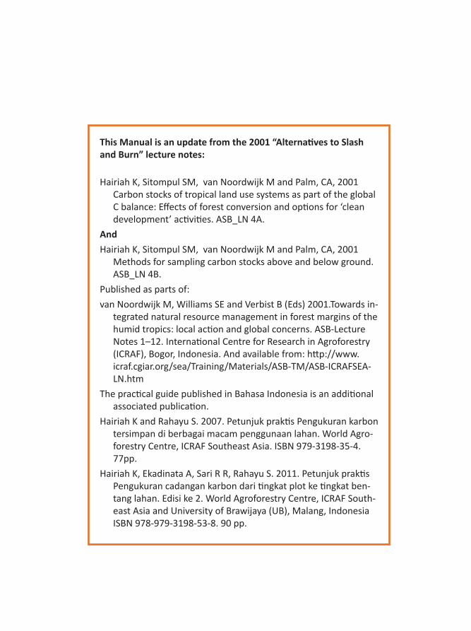
in which organic compounds are decomposed, absorbing O2 in the process of respira on.
a. Annual cycles
Through other metabolic processes, plants may convert sugars into starch, proteins, fats, cellulose or lignin in cell walls and woody structures. Most plants will first invest in the growth of roots and stems to allow their leaves to capture more light and capture more CO2. Once light capture is secured, plants may start to store starch and other organic compounds to survive adverse periods (for example, a dry or cold season) and/or to invest in reproduc on through flowers, pollen and seed produc on. The net balance between photosynthesis and respira on thus shi s during an annual cycle, and measurements of the net capture or release of CO2 by vegeta on will give different results in different seasons.
Animals obtain their carbon by ea ng and diges ng plants, so carbon moves through the bio c environment through the tropics system. Herbivores eat plants but are themselves eaten by carnivores. Parts of dead plants and organic waste and dead bodies of animals return to the soil, for further steps in decomposi on and respira on.
Box 2. What is photosynthesis?
Photosynthesis is the process by which green plants use carbon dioxide (CO2), water (H2O) and sunlight to make their own food. The word photosynthesis means “to put together with light”. When all these components are put together they make sugar and oxygen (O2).
Photosynthesis diagram Figure 3. (available from: h p://bioweb.uwlax.edu/bio203/s2008/brooks)

Measuring Carbon Stocks
6
Plants take in carbon as CO2 through the process of photosynthesis and convert it into sugars, starches and other materials necessary for the plant’s survival. From the plants, carbon is passed up the food chain to all the other organisms. This occurs when animals eat plants and when animals eat other animals.
Photosynthesis removes CO2 from the air and adds oxygen, while cellular respira on removes oxygen from the air and adds CO2. The processes generally balance each other out.
Both animals and plants release CO2 as a waste product. This is due to a process called cell respira on, where the cells of an organism break down sugars to produce energy for the func ons they are required to perform. The equa on for cell respira on is:
Glucose + Oxygen → Energy + Water + Carbon Dioxide
for example, C6H12O6 + 602 → Energy + 6H2O + 6CO2
CO2 is returned to the atmosphere when plants and animals die and decompose. The decomposi on releases CO2 back into the atmosphere where it will be absorbed again by other plants during photosynthesis. In this way, the cycle of CO2 being absorbed from the atmosphere and being released again forms a never-ending cycle.
In the carbon cycle, the amount of carbon in the environment always remains the same. However, in the last 200 years, the
burning of fossil fuels and deforesta on has increased the amount of atmospheric carbon dioxide from 0.028 to 0.035% and the concentra on is con nuing to increase. The increase in CO2 is accompanied by an equivalent decrease in the O2 concentra on, but because the O2 concentra on is so much higher (above 20% of the atmosphere), this decline is hardly no ceable and not of any real concern.
Con nued…

Measuring Carbon Stocks
7
b. Decadal pa erns of buildup of woody vegeta on
Perennial plants live for more than a year and may live for more than 100 years. They con nue to build up carbon stocks, mostly in woody stems and roots. Carbon storage increases during the process of vegeta on succession, when woody plants take over from herbs and shrubs, and when large trees take over from smaller ones. Ul mately, however, even big trees die and fall down, crea ng gaps in the vegeta on that allow other trees-in-wai ng to take over. The C cycle con nues, but one has to measure over the life cycle of trees to understand the net balance of sequestra on and respira on of natural (or man-made) vegeta on.
c. Century-scale build up of peat soils
Carbon captured in photosynthesis can move from the vegeta on into the soil. This happens first of all during the growth of roots, which form the basis of a belowground food web through fungi, bacteria and all the animals that feed on them. Part of the soil fauna is also able to incorporate dead leaves into the soil and the soil becomes ghtly linked with the li er layer on top that is formed by dead leaves and other parts of plants such as twigs, flowers or fruits. While in the end, much of the plant-derived organic ma er is respired in this food web, part of the organic material develops a chemical form that resists decomposi on or becomes ghtly bound to clay or silt par cles and thus is protected from decomposi on. Under condi ons that are s ll not fully understood, the decomposi on is so much slower than the rate of fresh organic inputs that peat layers start to build up, even under warm and humid condi ons, but assisted by high water tables and a low supply of oxygen. As peat soils have a low pH and low nutrient content, the subsequent organic inputs will decompose more slowly and the process of peat forma on can be reinforced. The buildup of peat soils can take centuries or thousands of years, and despite the low rates of plant growth, peat vegeta on is one of the most effec ve long term C storage mechanisms.
*) The Global Carbon Budget is zero. Its components, however, are of interest, as they balance the exchanges (incomes and losses) of carbon between the carbon reservoirs or between one specific loop (for example, atmosphere↔biosphere) of the carbon cycle. An examina on of the carbon budget of a pool or reservoir can provide informa on about whether the pool or reservoir is func oning as a source or sink for carbon dioxide.

Measuring Carbon Stocks
8
1.1.3 Carbon sequestra on at mul ple scales
The representa on of mul ple me scales (elaborated in sec on 1.2.2, the analysis of carbon budgets) can be done at mul ple temporal scales, but the results need to be interpreted differently. The different scales are indicated by acronyms such as GPP, NPP, NEP and NBP (see Figure 4B quoted from IPCC, 2000), as follows:
Gross Primary Produc on (GPP) • denotes the total amount of C fixed in the process of photosynthesis by plants in an ecosystem, such as a stand of trees. GPP is measured on photosynthe c ssues, principally leaves, on an hourly mescale and integrated to an annual amount. Global total GPP is about 120 Gt C yr-1.
Net Primary Produc on (NPP)• denotes the net produc on of organic ma er by plants in an ecosystem. NPP is about half of GPP as plants respire the other half in building up and maintaining plant ssues. NPP can be measured as the increase in plant biomass on a daily or weekly
mescale. For all terrestrial ecosystems combined, it is es mated to be about 60 Gt C yr-1.
Net Ecosystem Produc on (NEP)• denotes the net accumula on of organic ma er or C by an ecosystem; NEP is the difference between the rate of produc on of living organic ma er and the decomposi on rate of dead organic ma er (heterotrophic respira on). Heterotrophic respira on includes losses by herbivore and the decomposi on of organic ma er by organisms. Global NEP is es mated to be about 10 Gt C yr-1. NEP can be measured in two ways: one is to measure changes in C stocks in vegeta on and soil over me, using an annual mescale; the other is to integrate hourly/daily fluxes of CO2 into and out of vegeta on and integrate up to the yearly mescale. NEP should be integrated up to a decadal (10 year)
mescale.
Net Biome Produc on (NBP)• denotes the net produc on of organic ma er in a region containing a range of ecosystems (a biome) and includes, in addi on to heterotrophic respira on, other processes leading to loss of living and dead organic ma er (harvest, forest clearance and fire, among others). Compared to the total fluxes between the atmosphere and biosphere, global NBP is compara vely small at 0.7–1.0 Gt C yr-1. It can be measured only at a decadal or longer me frame, as the disturbances

Measuring Carbon Stocks
9
that are to be taken into account do not occur every year. The dis nc on between disturbances which are natural and those which are at least partly caused by humans is complex, especially where fire is involved.
The mescale selected for measurements is cri cal for the interpreta on of results. The scale of Net Ecosystem Produc vity is most appropriate in discussing the impacts of land cover/land use change on global emissions for two reasons. First, even though net biome produc vity (NBP) is most relevant in terms of mescale for global change debates, in order to calculate NBP it is necessary to measure the net ecosystem produc vity (NEP) and account separately for the disturbances (including harvests) which usually happen over a shorter mescale than a decade. This also relates to the me frame of climate change mi ga on ac ons and strategies under interna onal agreements; a decade is simply too long and hardly relevant. Secondly, it is feasible to calculate NEP for a large area and technically op mal regarding the uncertainty level. If C fluxes are measured on an hourly basis as gross primary produc vity (GPP) and plant respira on, then it is necessary to deal with very large numbers in either direc on. This measurement is not feasible if a large area of interest is to be covered, not to men on global analysis. In addi on, the uncertain es in the measurements will make it difficult to assess the small differences between losses and gains.
Net ecosystem produc vity (NEP) can be assessed as a me-averaged C stock of the system (Hairiah et al., 2001; IPCC-LULUCF (sec on 4), 2000), or ‘typical C stock’ (White et al., 2010. Time-averaged C stocks of a land use system records the amount of C stocks that are actually present in situ, averaged over the life cycle of such a land use system. The key then is to be able to quan fy the current (on-site) C stock at any stage of the life cycle of a land use system and scale up to the typical life cycle. At this mescale, many fluxes can be expected to cancel out and we can focus on net changes to the bo om line. Time-averaged C stock is discussed in Part II.

Measuring Carbon Stocks
10
1.1.4 Special roles of forest?
The vegeta on of tropical forest is a large and globally significant storage of C because tropical forest contains more C per unit area than any other land cover. The main carbon pools in tropical forest ecosystems are the living biomass of trees and understory vegeta on and the dead mass of li er, woody debris and soil organic ma er. About 50% of plant biomass consists of C. The carbon stored in the aboveground living biomass of trees is typically the largest pool and the most directly impacted by deforesta on and degrada on.
The C stock in an individual tree depends on the tree’s size. For trees of 10, 30, 50 or 70 cm stem diameter (measured at a standard 1.3 m above the ground and known as the diameter at breast height or DBH), the biomass may be around 135, 2250, 8500 or 20,000 kg/tree, respec vely. A forest with stocking of 900, 70, 20 and 10 such trees per ha, will have a total biomass of 645 Mg ha-1, with a corresponding C stock of 290 Mg ha-1, with 19, 24, 26 and 31% in the respec ve diameter classes. Most of the biomass is in the few really big trees.
Cu ng down trees in the forest releases C to the atmosphere. Although selec ve logging may only remove a few big trees per area (and damage surrounding ones), it can lead to a substan al decrease in total biomass and C stock.
Large trees tend to have large roots. For mixed tropical forest, the ra o of aboveground to belowground biomass is approximately 4:1; in very wet condi ons, the ra o can shi upwards to 10:1, while under dry condi ons it may decrease to 1:1 (van Noordwijk et al., 1996, Houghton et al., 2001, Achard et al., 2002, Ramanku y et al., 2007 et al.). As measurement of root biomass is not simple (Smit et al., 2000) there is a method that uses the root diameter at stem base and allometric equa ons (van Noordwijk and Mulia, 2002), default assump ons are normally used for the shoot:root ra o based on literature reviews (van Noordwijk et al., 1996; Cairns et al., 1997; Mokany et al., 2006).
When forests (with an average of 250 Mg C ha-1) are transformed to agricultural ac vi es, the subsequent land use systems implemented determine the amount of poten al carbon restocking that takes place. On average, annual crop systems will contain only 3 Mg C ha-1 and intensive tree crop planta ons 30–60 Mg C ha-1 (Tomich et al., 1998; Palm et al., 2005), or 1 and 10–25% of the forest biomass and C stock, respec vely. The annual

Measuring Carbon Stocks
11
C sequestra on rate (increment of standing stock) may be the same (about 3 Mg C ha-1 yr-1) for all three vegeta on types (annual crop, tree planta on and forest), but the mean residence me differs from 1, 10 to 83 years, respec vely. Changes in C stock between vegeta on and land use types relate primarily to this mean residence me.
Thus, es ma ng aboveground forest biomass carbon is the cri cal step in quan fying carbon stocks and fluxes from tropical forests. Root biomass is es mated to be 20% of the aboveground forest carbon stocks for most forest types, but it can be less than 10% or more than 90% in specific vegeta on types (for example, Houghton et al., 2001, Achard et al., 2002, Ramanku y et al., 2007; van Noordwijk et al., 1996) based on a predic ve rela onship established from extensive literature reviews (Cairns et al., 1997, Mokany et al., 2006). Reliable es mates of biomass, li er and soil carbon are needed to understand the effect of forests on atmospheric carbon dioxide. Forest inventories that focus on harvestable mber o en need to be augmented to quan fy the whole carbon budget of the forest (Figure 4).
(A) Illustra on of forest inventory-based approach to es mate carbon budgets, Figure 4. where es mates of stem volume of growing stock, gross increment and fellings are converted to biomass, which is further converted to li erfall with turnover rates and the es mated li erfall is fed into dynamic soil carbon. This approach gives directly es mates of changes in the carbon stock of trees and forest soil (available from: h p://www.helsinki.fi/geography/research )
(A)

Measuring Carbon Stocks
12
(B) Equivalent terms as used in Forestry and Ecological research.Figure 4.
For the same reason, trees growing either inside or outside the forest take up C from the atmosphere and store it as biomass for a long me. Natural forests can reach a biomass equilibrium stage when the collapse of a big tree matches the growth of the smaller trees surrounding it, but tree mortality tends to be concentrated in years of excep onal weather. Total biomass shi s up and down at a patch level but is approximately constant at the level of a forest or forested landscape in the absence of logging and other human disturbance. In prac ce, however, many forests are s ll recovering from previous levels of human exploita on as well as natural disturbance.
While old-growth forests have the highest aboveground C stock, they usually have a low rate of further C sequestra on. Other forests (‘younger’ in ecological terms) may have less C stock (Box 3), but a higher rate of accumula on. Grasslands and pioneer vegeta on may have the highest rate of C gross primary produc vity, but low stocks and low inter-annual increment in storage. However, given this range, there is no reason to treat forests differently from other vegeta on types in the assessment of terrestrial C stocks. There should be no confusion regarding the me frame over which comparisons are to be made.
(B)

Measuring Carbon Stocks
13
Box 3. Case study: Measurement of C stocks of different land use types
Aboveground carbon storage in natural forest is higher than that in any other vegeta on, but total C storage can be higher in peat ecosystems (with or without forest). Based on methods that will be explained in Part 2, an overview of C stocks in different land use systems in the humid tropics was obtained by ASB scien sts in the early 1990’s (Figure 5).
The magnitude of losses and poten al C sequestra on with transi ons between the various land uses can be es mated from the summary data. For example, C losses from conver ng natural forests to logged forests range from a low of 80 Mg C ha-1 to a high of 200 Mg C ha-1. The majority of the C is lost from the vegeta on with li le loss from the soil. If the logged forests are further converted to con nuous cropping or pasture systems, an addi onal 90 to 200 Mg C ha-1 are lost aboveground and 25 Mg C ha-1 are lost from the topsoil. Losses from conversion of logged forests to other tree-based systems are smaller, from 40 to 180 Mg C ha-1 aboveground and 10 Mg C ha-1 from the soil. If croplands and pastures were rehabilitated through conversion to tree-based systems, then this would result in net carbon sequestra on. Over a 25-year period, the amount of C that could be sequestered would range from 5 to 60 Mg C ha-1 aboveground and 5 to 15 Mg C ha-1 in the topsoil. The main point is that the poten al for C sequestra on in the humid tropics is aboveground, not in the soil.
Figure 5. Aboveground me-averaged carbon stocks and total soil C (0–20 cm) for land uses in benchmark sites in Indonesia, Cameroon and Brazil. Details of data collec on are explained in Part 2.

Measuring Carbon Stocks
14
1.2. Interna onal agreements1.2.1 United Na ons Framework Conven on on Climate
Change
A total of 192 countries in the world have joined an interna onal treaty—the United Na ons Framework Conven on on Climate Change (UNFCCC)—to begin to consider what can be done to reduce global warming and to cope with whatever temperature increases are inevitable.
Box 4. Adapta on and mi ga on to climate change
The ul mate objec ve of the United Na ons Framework Conven on on Climate Change (UNFCC) and any related legal instruments that the Conference of the Par es (COP) may adopt is to achieve, in accordance with the relevant provisions of the Conven on, stabiliza on of greenhouse gas concentra ons in the atmosphere at a level that would prevent dangerous anthropogenic interference with the climate system. Such a level should be achieved within a me frame sufficient to allow ecosystems to adapt naturally to climate change, to ensure that food produc on is not threatened and to enable economic development to proceed in a sustainable manner.
Most, but not all, na ons have also approved an addi on to the treaty: the Kyoto Protocol, which entered into force on 16 February 2005 and which has more powerful (and legally binding) measures, focused on the first commitment period of 2008–2012.
The Conven on places the heaviest burden for figh ng climate change on industrialized na ons, since they are the source of most past and current greenhouse gas emissions. These countries are asked to do the most to cut what comes out of smokestacks and tailpipes, and to provide most of the money for efforts elsewhere. For the most part, these developed na ons (called Annex I countries because they are listed in the first annex to the treaty) belong to the Organiza on for Economic Coopera on and Development (OECD). These advanced na ons, as well as 12 “economies in

Measuring Carbon Stocks
15
transi on” (countries in Central and Eastern Europe, including some states formerly belonging to the Soviet Union) were expected by the year 2000 to reduce emissions to 1990 levels. As a group, they succeeded. Industrialized na ons agreed under the Conven on to support climate-change ac vi es in developing countries by providing financial support above and beyond any financial assistance they were already providing to these countries. Because economic development is vital for the world’s poorer countries—and because such progress is difficult to achieve even without the complica ons added by climate change—the Conven on accepts that the share of greenhouse gas emissions produced by developing na ons will grow in the coming years. Nonetheless, it seeks to help such countries limit emissions in ways that will not hinder their economic progress. The Conven on acknowledges the vulnerability of developing countries to climate change and calls for special efforts to ease the consequences. While developing countries have not so far agreed to commit themselves to any level of emissions (per capita or per country), they have an obliga on to report their emissions and C stocks to assist in the global bookkeeping of emissions and the drivers of climate change. Developing countries that want to par cipate in other mechanisms of the Conven on will need to provide such data, as part of global transparency.
1.2.2 IPCC repor ng standards Par es to the Conven on must submit na onal reports on the implementa on of the Conven on to the Conference of the Par es (COP), in accordance with the principle of “common but differen ated responsibili es” enshrined in the Conven on. The core elements of the na onal communica ons for both Annex I and non-Annex I Par es are informa on on emissions and removals of greenhouse gases (GHGs) and details of the ac vi es a Party has undertaken to implement the Conven on. Na onal communica ons usually contain informa on on na onal circumstances, vulnerability assessment, financial resources, transfer of technology, educa on, training and public awareness, but the ones from Annex I Par es addi onally contain informa on on policies and measures. Annex I Par es are required to submit informa on on their na onal inventories annually and to submit na onal communica ons periodically, according to dates set by the COP. There are no fixed dates for the submission of na onal communica ons by non-Annex I Par es, although these documents should be submi ed within four years of the ini al disbursement of financial resources to assist them in preparing their na onal communica ons.

Measuring Carbon Stocks
16
Box 5. Formal obliga ons as part of the UNFCCC conven on
Ar cle 4, paragraph 1(a): Develop, periodically update, publish and make available to the Conference of the Par es, in accordance with Ar cle 12, na onal inventories of anthropogenic emissions by sources and removals by sinks of all greenhouse gases (GHGs)* not controlled by the Montreal Protocol, using comparable methodologies to be agreed upon by the Conference of the Par es.
(* including inventories of GHG emissions and removals from the LULUCF sector)
Ar cle 4, paragraph 1(d): Promote sustainable management, and promote and cooperate in the conserva on and enhancement, as appropriate, of sinks and reservoirs of all GHGs not controlled by the Montreal Protocol, including biomass, forests and oceans as well as other terrestrial, coastal and marine ecosystems
Accurate, consistent and interna onally comparable data on GHG emissions is essen al for the interna onal community to take the most appropriate ac on to mi gate climate change and ul mately to achieve the objec ve of the Conven on. Communica ng relevant informa on on the most effec ve ways to reduce emissions and adapt to the adverse effects of climate change also contributes towards global sustainable development.
The first global guidelines for repor ng on the land use component were interna onally agreed in 1996 as “LULUCF” (land use, land use change and forestry). This was followed in 2003 by the “Good Prac ce Guidance for Land Use, Land Use Change and Forestry” (GPG-LULUCF) as the response to the invita on by the United Na ons Framework Conven on on Climate Change (UNFCCC) to the Intergovernmental Panel on Climate Change (IPCC) to develop good prac ce guidance for land use, land use change and forestry (LULUCF).
A revised version that ironed out some inconsistencies was ra fied in 2006 as “AFOLU” (agriculture, forestry and other land uses). The categories within the good prac ce guideline (GPG) for different land uses are presented in Box 5, in which non-ambiguous land categories are assumed. However, in prac ce, these o en s ll present some confusion and inconsistency. For example,

Measuring Carbon Stocks
17
where does a rubber agroforest on peatland belong? It meets the minimum tree height and crown cover of forest, but is on a wetland and its produc on is recorded under agricultural sta s cs. Consistency of accoun ng methods across land categories requires a good understanding of such rela ons.
Box 6. Levels of sophis ca on ( ers) in GHG accoun ng
The 2006 IPCC Guidelines for Na onal Greenhouse Gas Inventories Volume 4 Agriculture, Forestry and Other Land Use (h p://www.ipcc-nggip.iges.or.jp/public/2006gl/vol4.html) provided a framework 3- ered structure for AFOLU (Agriculture, Forestry and Other Land Use is the name for historical reasons; it might just as well be called ‘all land use’) methods:
“Tier 1 methods are designed to be the simplest to use, for which equa ons and default parameter values (e.g., emission and stock change factors) are provided in this volume. Country-specific ac vity data are needed, but for Tier 1 there are o en globally available sources of ac vity data es mates (e.g., deforesta on rates, agricultural produc on sta s cs, global land cover maps, fer lizer use, livestock popula on data, etc.), although these data are usually spa ally coarse.”
“Tier 2 can use the same methodological approach as Tier 1 but applies mission and stock change factors that are based on country- or region-specific data, for the most important land use or livestock categories. Country-defined emission factors are more appropriate for the clima c regions, land use systems and livestock categories in that country. Higher temporal and spa al resolu on and more disaggregated ac vity data are typically used in Tier 2 to correspond with country-defined coefficients for specific regions and specialized land use or livestock categories.”

Measuring Carbon Stocks
18
“At Tier 3, higher order methods are used, including models and inventory measurement systems tailored to address na onal circumstances, repeated over me, and driven by high-resolu on ac vity data and disaggregated at sub-na onal level. These higher order methods provide es mates of greater certainty than lower
ers. Such systems may include comprehensive field sampling repeated at regular me intervals and/or GIS-based systems of age, class/produc on data, soils data, and land use and management ac vity data, integra ng several types of monitoring. Pieces of land where a land use change occurs can usually be tracked over me, at least sta s cally. In most cases these systems have a climate dependency, and thus provide source es mates with inter-annual variability. Detailed disaggrega on of livestock popula on according to animal type, age, body weight etc., can be used. Models should undergo quality checks, audits, and valida ons and be thoroughly documented.”
The current Manual is intended to provide data that can be summarized for Tier 2 approaches, or feed into more sophis cated Tier 3 methodology.
Box 7. Six land categories
(i) Forest Land
This category includes all land with woody vegeta on consistent with thresholds used to define Forest Land in the na onal greenhouse gas inventory. It also includes systems with a vegeta on structure that currently fall below (but in situ could poten ally reach) the threshold values used by a country to define the Forest Land category.
(ii) Cropland
This category includes cropped land, including rice fields, and agro-forestry systems where the vegeta on structure (current or poten ally) falls below the thresholds used for the Forest Land category.
Con nued…

Measuring Carbon Stocks
19
(iii) Grassland
This category includes rangelands and pasture land that are not considered Cropland. It also includes systems with woody vegeta on and other non-grass vegeta on such as herbs and brush that fall below the threshold values used in the Forest Land category. The category also includes all grassland from wild lands to recrea onal areas as well as agricultural and silvi-pastoral systems, consistent with na onal defini ons.
(iv) Wetlands
This category includes areas of peat extrac on and land that is covered or saturated by water for all or part of the year (such as peatlands) and that does not fall into the Forest Land, Cropland, Grassland or Se lements categories. It includes reservoirs as a managed subdivision and natural rivers and lakes as unmanaged subdivisions.
(v) Se lements
This category includes all developed land, including transporta on infrastructure and human se lements of any size, unless they are already included under other categories. This should be consistent with na onal defini ons.
(vi) Other Land
This category includes bare soil, rock, ice and all land areas that do not fall into any of the other five categories. It allows the total of iden fied land areas to match the na onal area, where data are available. If data are available, countries are encouraged to classify unmanaged lands by the above land use categories (for example, into Unmanaged Forest Land, Unmanaged Grassland, and Unmanaged Wetlands). This will improve transparency and enhance the ability to track land use conversions from specific types of unmanaged lands into the categories above.
Con nued…
Measuring Carbon Stocks
20
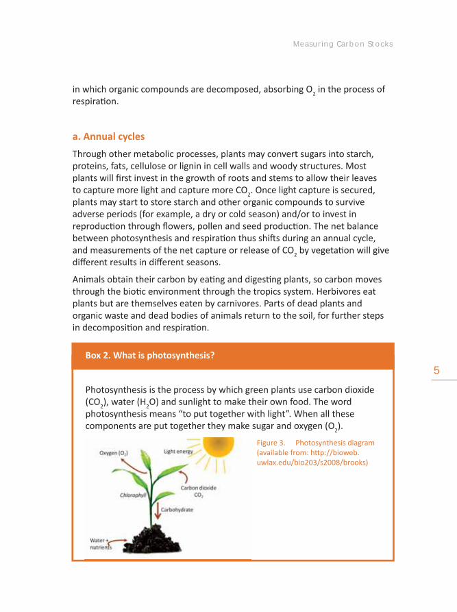
1.2.3 Kyoto Protocol, Bali roadmap, RE(D)i+j
Forest carbon (C) sinks were included in the Kyoto Protocol as a mechanism to mi gate global climate change. According to the Protocol, the net sink of C arising from land use changes and forestry over the period 2008–2012 can be credited and may be considered as a reduc on of GHG emissions to fulfill the repor ng requirements in the interna onal agreements of Annex I countries.
However, for developing countries, only one category of the various land use changes is eligible as mi ga on ac on—namely, afforesta on/reforesta on (A/R)—that can be part of the Clean Development Mechanism (CDM), but under strict regula on. In prac ce, such A/R-CDM approaches have been difficult to ini ate and get approved, both at the na onal and the interna onal level.
Meanwhile, the losses due to tropical deforesta on con nued unabated. At the 13th Conference of Par es in Bali in December 2007 a “Bali Road Map” was agreed upon which contained efforts to include a new mechanism for reducing emissions from deforesta on and forest degrada on (REDD) in the agreements that were to define the successor of the Kyoto Protocol, at the 15th COP in Copenhagen (2009) and lead to par al agreement in Cancun (2010).
In the Kyoto Protocol, only a small subset of the issues regarding land use was recognized as mi ga on ac on and incorporated via the A/R-CDM mechanism.
Components of global climate agreements required to deal with emission Figure 6. reduc on and allevia on of rural poverty; SFM = Sustainable Forest Management, SLM = Sustainable Land Management, Agric. = Agricultural.

Measuring Carbon Stocks
21
Current efforts on REDD and sustainable forest management (SFM) broaden the reach, but the cross-sectoral linkages in land use within the comprehensive AFOLU umbrella have probably not received enough a en on (Figure 6). Forests have been singled out for priority ac on, but the forest defini on is too fuzzy for clear delinea on of what is ‘in’ and what is ‘out’1 (van Noordwijk and Minang, 2009).
The current framing of the efforts to reduce emissions from deforesta on and degrada on (REDD) refers to a par al accoun ng of land use change, without clarity on crosssectoral linkages and rights other than those of forestry authori es. Nego a on processes to add safeguards will likely slow down and complicate implementa on. A more compre-hensive and rights-based approach to reducing emissions from any land use, reducing emissions from any land use, (REALU), embedding REDD efforts, is likely to be more effec ve. This can be based on the totality of AFOLU accoun ng.
The progression of issues to be included in the RED → REDD → REDD+ → REDD++ (or in shorthand nota on RE(D)i
+j for i=1,2 and j=0,1,2) is reflected in the parts of a land cover change matrix that is to be included in the calcula ons of emissions.
1 h p://www.redd-monitor.org/2008/12/17/forest-defini on-challenged-in-poznan/
Rela onships between REDD and other components of AFOLU Figure 7. (agriculture, forestry and other land uses) emissions of greenhouse gases, such as peatlands, restoring C stocks with trees and soil C and emissions of CH4 and N2O (agricultural greenhouse gases or AGG).

Measuring Carbon Stocks
22
RED Reducing emissions from (gross) deforesta on: only changes from forest to non-forest land cover types are included, and details very much depend on the opera onal defini on of ‘forest’.
REDD REDD + (forest) degrada on, or the shi s to lower C stock densi es within the forest; details very much depend on the opera onal defini on of ‘forest’.
REDD+ REDD+ + restocking within and towards ‘forest’; in some versions, REDD+ will also include peatland, regardless of its forest status; details s ll depend on the opera onal defini on of ‘forest’.
REDD++ REALU = REDD++ + all transi ons in land cover that affect C storage, whether peatland or mineral soil, trees-outside-forest, agroforest, planta ons or natural forest. It does not depend on the opera onal defini on of ‘forest’, but on consistency in the overall land cover stra fica on scheme.
Defini on of Forest
The forest defini on accepted by the interna onal community (Box 6) has a number of counter-intui ve consequences, such as:
There is no issue of deforesta on in the conversion to oil palm planta ons, A) as such planta ons meet the defini on of forest.
There is no deforesta on in a country like Indonesia, as land remains B) under the ins tu onal control of forest ins tu ons and is only ‘temporarily unstocked’.
Swiddening and shi ing cul va on can be finally removed from the list of C) drivers of deforesta on, as long as the fallow phase can be expected to reach minimum tree height and crown cover.
Most tree crop produc on and agroforestry systems do meet the D) minimum requirements of forest; for example, unpruned coffee can easily reach a height of 5 m.

Measuring Carbon Stocks
23
The current transforma on of natural forest, a er rounds of logging, into E) fastwood planta ons (Cossalter, 2003) occurs fully within the ‘forest’ category, out of reach of RED policies.
Large emissions of peatland areas that have lost forest cover and were F) excised from the ‘forest’ estate do not fall under forest-related emission preven on rules, if the conversion happened before the cut-off date (yet to be specified).
Substan al tree-based land cover types fall outside of the current G) ins tu onal frame and jurisdic on of ‘forests’, and require broad-based implementa on arrangements.
Probably there is no single defini on of forest that can provide a clear dichotomy in the con nuum of landscapes with trees. From a biodiversity perspec ve, a cutoff between ‘natural’ and ‘planted’ forest may seem desirable, but again there are many intermediate forms.
For issues of C accoun ng, defini ons or terminology should not cause any fuzziness as long as a number of dis nc ons are made among the ‘woody vegeta on’ components that are actually found on the land (including ‘trees outside forest’) and link measurements on the ground to maps that use consistent classifica ons. However, in terms of local and na onal policy, there are four broad classes of land (see Figure 8):
Four basic classes of land with respect to presence of trees and ins tu onal Figure 8. forest claims.

Measuring Carbon Stocks
24
Forest with trees;1.
Forest without trees, but included in the ‘ins tu onal’ forest based on 2. expecta ons that trees will or should be present;
Trees outside ‘ins tu onal’ forest, above or below the threshold for tree 3. height and crown cover;
Non-forest without trees.4.
This Manual deal with all land cover without discrimina on. Terms such as ‘deforesta on’ can be be er replaced by ‘changes in tree cover’ or ‘aboveground C stock’, to avoid the policy complica ons of the word ‘forest’ and its deriva ves.
The various types of REDi+j accoun ng schemes can now be interpreted as different ways (or filters) of processing data on land cover change. A 10-step classifica on of land cover can be used: 1. Natural forest; 2. Logged-over forest high density; 3. Logged-over forest medium density; 4. Agroforest (managed + natural tree establishment); 5. Fastwood planta on; 6. Tree crop planta on; 7. Half-open agroforestry, heavily logged forest and shrub; 8. Open-field crops; 9. Grassland; 10. Urban areas + roads. Adop ng this classifica on, the parts of the change matrix can be selected that will be included in the accoun ng scheme for different rules (Figure 9).

25
Land
use
cha
nge
mat
rix
and
cells
(refl
ecng
dec
reas
e or
incr
ease
in C
sto
ck o
ver
a m
e pe
riod
bet
wee
n tw
o ob
serv
aon
s) th
at c
an
Figu
re 9
. be
incl
uded
in a
rang
e of
pos
sibi
le R
ED s
chem
es.

Measuring Carbon Stocks
26
Box 8. Forests—what’s in a name?
What is a forest? What is not a forest? The history of the term (‘sylva fores s’ in La n) suggests that it is not the equivalent of woody vegeta on (‘sylva’) but rather with that part that is ‘outside reach’ or ‘fores s’. This qualifier became the shorthand form. Forests have always been defined by reference to an ins tu on, for example, the king, (or ‘crown’) who claims control over it, not based on the presence or absence of trees. The ‘king’ has been replaced by ‘forestry departments’ of various forms in different countries, but the dichotomy between village/community and forest has usually remained. Villagers will not voluntarily describe their tree-based vegeta on as a forest, as this implies a risk of denial of their rights and ‘trouble’.
The forest defini on agreed on by the UNFCCC in the context of the Kyoto Protocol has three significant parts, only one of which has received a lot of a en on:
1) Forest refers to a country-specific choice for a threshold canopy cover (10–30%) and tree height (2–5 m); the choice of these thresholds has been widely discussed.
2) The above thresholds are applied through ‘expert judgement’ of ‘poten al to be reached in situ’, not necessarily to the current vegeta on
3) Temporarily unstocked areas remain ‘forest’ as long as a forester thinks they will, can or should return to tree cover condi ons.
Rules 2 and 3 were added to restrict the concept of reforesta on and afforesta on and allow ‘forest management’ prac ces including clear felling followed by replan ng to take place within the forest domain. They make the direct observa on of ‘forest’ difficult. There is no me limit to ‘temporarily’.

Measuring Carbon Stocks
27
1.3 Measuring C stock in less uncertain ways
Es ma ng the carbon stock on an area can be achieved by taking a representa ve sample rather than measuring the carbon in all components over the whole area. A small, but carefully chosen sample can be used to represent the popula on. The sample reflects the characteris cs of the popula on from which it is drawn. For carbon sampling, measurements should be accurate (close to reality for the en re popula on) and precise (short confidence intervals, implying low uncertainty).
1.3.1. Accuracy: bias and precisionThe final value calculated from any sampling or accoun ng method will probably differ from the actual value at the me of assessment. While this is unavoidable, it is important to realize the consequences of inaccurate answers and the costs involved in ge ng be er and be er approxima ons. It is useful to dis nguish between two sources of ‘inaccuracy’ (the difference between the es mate and the actual value)—namely, bias (systema c error) and incomplete sampling (random error)—as shown in Figure. 10. Only incomplete sampling can be dealt with by increasing the sampling effort. Bias can derive from the use of inaccurate or wrongly calibrated methods and equa ons, or from sampling schemes that give a higher probability of inclusion in the sample to areas with either a rela vely low or a rela vely high value.
The varia on between replicates can be used to es mate the precision of the sample mean, but it does not reflect its accuracy, as any bias is not revealed. Bias may only show up if data from mul ple sources are compared with measurements at another scale. When the first es mates of the global C cycle were made (see Figure 1), there were large amounts of ‘missing carbon’ due to inconsistencies in methods used by the various data sources. A number of sources of bias in the data collec on have since been iden fied and the data gap is smaller but it s ll exists. In the context of policies and interna onal regula on, bias and precision play different roles. Rela ve, (rather than absolute) changes in emissions and stocks are the targets of such policies. Thus, as long as bias is consistent in space and me, it does not affect the policy process. However, inconsistencies between the outcomes of different methods can be used as an excuse for inac on (”the scien sts don’t yet agree, so we had be er wait”). Random error tends to be smaller at a na onal

Measuring Carbon Stocks
28
scale of data aggrega on than at sub-na onal units where fewer samples are involved. This is important for the scales of policy instruments. If changes in C stocks in rela vely small areas are the target of a project, a substan al sampling effort will be needed to quan fy those changes in C stocks for the area. If the target changes at a na onal scale, a similar effort spread over a much larger area might suffice to obtain the same precision at much lower cost per unit change in the C stock measured. The emphasis on precision at project scales may have contributed to the impression that C accoun ng at the na onal scale will be complicated and expensive. It does not have to be, if efficient sampling schemes are used. Poli cal processes, however, don’t readily appreciate sta s cal arguments, and may want to see detailed ‘wall-to-wall’ evidence before ac on is taken. The psychology and art of communica on are as important as the accuracy and precision of the data.
Lack of precision and bias can both lead to inaccurate es mates but only the first Figure 10. can be dealt with by increasing the number of samples. Assuming the objec ve is to sample the bulls eye in the centre of the target: (A) all sampling points, while close to the centre, will have low bias, but they are widely spaced and therefore have low precision; (B) all points are closely grouped indica ng precision but they are far from the center and so are biased and inaccurate; (C) all points are close to the center and closely grouped, so they are precise and unbiased or in a word, accurate.

Measuring Carbon Stocks
29
1.3.2. Stra fied sampling through remote sensing Carbon accoun ng makes use of stra fied sampling and has the classical benefits and drawbacks of such an approach, when compared to a random sampling approach. In this case, stra fica on refers to the division of a heterogeneous landscape into dis nct strata based on the carbon stock in the vegeta on.
The benefits are:
If the strata are well defined and internally homogeneous (rela ve to the • total popula on), the number of samples required to achieve a specified accuracy of the mean is considerably smaller than with random sampling.
This benefit is especially pronounced if rela vely small strata represent • high values that will be hard to correctly represent in random sampling efforts.
The method is more robust if the overall distribu on does not follow a • normal probability distribu on, but s ll assumes devia ons from such a distribu on within each stratum are manageable.
The weaknesses are:
If stratum weights are not adequately known a priori or through other • means, stra fied sampling may be biased.
Sampling within each stratum should s ll be random (equal probability for • all elements in the stratum to be selected for observa on), which requires mapping or lis ng of all stratum elements.
In carbon accoun ng, maps derived from remote sensing (or direct a ributes at the unit or pixel scale) form the strata of a discrete number of land use/cover types. Classifica on errors (uncertainty of stratum weights) depend on the legend used, with generally higher precision on low carbon density landscapes and problema cal dis nc ons within high carbon density categories, but most likely the misclassifica on falls within similar carbon density categories.
If the area of interest is large enough resul ng in some biophysical factors that influence biomass accumula on (and therefore C stocks), such as climate and topography, not being homogeneous, then further stra fica on is necessary in order to reduce uncertainty. To avoid confusion, this manual refers to such stra fica on as zona on as opposed to stra fica on based on land use/cover types. Maps with appropriate scales to the extent of the area of interest are necessary to help in the design of an effec ve sampling procedure.

Measuring Carbon Stocks
30
Box 9. Steps to determine the number of sampling plots (adapted from Rugnitz et al., 2009)
Step 1. Select the desired level of accuracy
The selec on of the level of accuracy is almost always related to the resources available and the demands of the buyer (the market). The level of precision required will have a direct effect on inventory costs. Usually, the level of precision for forest projects (sampling error) is ±10% of the average carbon value with a level of confidence of 95%. Small-scale CDM forestry projects can use a precision level up to ±20% (Emmer 2007). However, specific levels of precision can be defined for each component of the inventory.
Figure 11 illustrates the rela onship between the number of plots and the level (degree) of accuracy ±% of the total carbon stock in living and dead biomass, with 95% confidence limits (Noel Kempff Project in Bolivia). To achieve an accuracy level of ±5%, 452 plots are needed, whereas only 81 plots would give a ±10% level of accuracy. This example illustrates the cost-benefit implica ons of a higher accuracy level.
Rela onship between number of plots and desired Figure 11. (or required) level of accuracy.

Measuring Carbon Stocks
31
Con nued…
Step 2. Select areas for preliminary data gathering
Before determining the number of plots required for the monitoring and measurement of carbon with a certain level of confidence, you must first obtain an es mate of the exis ng variance for each type of deposit (for example, soil carbon) in each land use system classified in the land use legend. Depending on the occurrence of the same stratum in the project area, each layer must be sampled over an area (repe on), so that results have sta s cal validity. Ini ally, it is recommended that a set of four to eight repe ons be used for each land use system.
Step 3. Es ma ng the average, standard devia on and variance of carbon stock preliminary data
The me-averaged C stock is calculated for each land use system or land use legend from the preliminary data (or obtained from the literature if studies in similar areas are available).
Output: Average, standard devia on and variance of carbon per land use system/legend.
Step 4. Calcula ng the required number of sampling plots
Once the variance for each land use system/legend, the desired level of precision and es mated error (referenced in the confidence level selected) are known, the number of sampling plots required can be calculated. The generic formulas for calcula ng the number of plots for different land systems are:
1) For one land use system:
Average Variance StandartDevia on

Measuring Carbon Stocks
32
2) For more than one land use system:
Where:
n = number of plots
E = allowed error (average precision × level selected). As seen in the previous step, the recommended level of accuracy is ± 10% (0.1) of the average but can be up to ±20% (0.2).
t = sta s cal sample of the t distribu on for a 95% level of confidence (usually a value of 2 is used)
N = number of plots in the area of the layer (stratum area divided by the plot size in ha)
s = standard devia on of the land use system
Online tools: Winrock Interna onal has developed an online Excel tool called the Winrock Terrestrial Sampling Calculator that helps in the calcula on of the number of samples and the cost involved for base line studies as well as monitoring.
(See: h p://www.winrock.org/ecosystems/tools.asp).
Con nued…

33
Carbon is also stored in the necromass (dead tree) for several years at least; it will gradually be released through decomposi on.
2photo: Kurniatun Hairiah


35
Part 2: How to do it?
2.1 Overview of Rapid Carbon Stock Appraisal (RaCSA)
The following research protocol on measuring C stocks was developed as part of the global ASB (Alterna ves to Slash and Burn) project to es mate C stocks at various levels in mineral soils and peat soils. The protocol was developed as a carbon accoun ng tool with stakeholders under the name Rapid Carbon Stock Appraisal (RaCSA). The discussion so far has looked at na onal accoun ng systems, but the basic data for RaCSA must come from efforts at a more local level to measure the carbon stocks in the landscape. Such a more localized assessment can be undertaken by following the RaCSA protocol. The basic steps of data collec on and measurement of trees are not par cularly difficult and do not require expensive or complex equipment, but consistency and a en on to detail are necessary. So far, much of the cost of carbon measurements has been in the design of the system and the costs for external experts to travel to remote loca ons rather than on the me spent actually measuring trees. Different ways of organizing these efforts can be substan ally more cost effec ve if local exper se can be developed and standards of repor ng and verifica on can be maintained.
With the increasing importance of carbon stock assessments in policy and the possible consequences for economic incen ves (C markets), it is relevant that local stakeholders are aware of and involved in data collec on and processing, so that they can deal with the ‘slick carbon cowboys’ and ‘carbon snake oil merchants’ that are exploi ng the current innocence and ignorance of local governments and communi es.
The RaCSA protocol includes three types of knowledge: local ecological knowledge (LEK), public/policy knowledge (PEK) and scien fic/modeling knowledge (MEK) (Figure 12; Photo 1). Comparing and contras ng these knowledge types involves the classifica on/stra fica on schemes as much

Measuring Carbon Stocks
36
as the measures of carbon stock density. The public/policy domain tends to focus on ins tu onal categories and associated departmental divisions rather than the actual vegeta on and carbon stocks involved. In using exis ng data sources, such as ‘forest cover’, the lack of clarity in opera onal defini ons used is a major problem. The main output of RaCSA is landscape carbon es mates under various scenarios of land use change, taking into account ways to measure ac vi es that are expected to improve local livelihoods and alleviate rural poverty.
Four main components and outputs under RaCSA approach.Figure 12.
Inventory of all land use systems managed by farmers (1) including discussion Photo 1. between researchers, farmers and governments, (2, 3, 4) on the dynamics of the landscape over me as a result of changes in the way people manage their natural resources.

Measuring Carbon Stocks
37
2.2. Concepts of carbon stock accoun ng and monitoring
The basis for area-based carbon stock accoun ng is an equa on to es mate the changes in carbon stock within and between land cover classes, with each characterized as a frac on (ai) of the total area (A) (the stratum weigh ng) and each with a me-dependent carbon stock density Ci,t (the stratum mean).
Where:
∆C = annual change in carbon stocks in the landscape in Mg yr-1 or t yr-1.
Carbon stock density consists of the aboveground and belowground biomass, above¬ground necromass and soil organic ma er. The total annual change of carbon stock at the landscape level is the sum of the area of each transi on of land uses mul plied by the total changes in C stock for each transi on per unit area, divided by the me period. The changes accounted for are net changes, that is, the sum of gains and losses. Gains are derived from vegeta on growth while losses can result from harvest, disturbance, decomposi on, combus on, fer liza on and drainage. When the calcula ons are applied to a large enough area of interest and over a long enough me period, a ‘ me-averaged stock’ approach to carbon can be applied that balances the gains and losses occurring at the year-by-year level during a typical life cycle.
The choices of system boundary (landscape extent or the coverage of the area of interest) and the me period should be made based on the specific objec ves of the research. The objec ves should also drive the level of accuracy that is to be achieved; accuracy should not be considered independently of the level of available resources. It is important to note that the summa on of the areas represents total areas, therefore this formula expresses a comprehensive accoun ng system rather than covering parts of the landscape, such as the natural forest only or areas designated to be a
change in average C stock
change in area for class i
))()(( ,,1,,1,1
,1 tititititi
n
itittt CaaCCaAC

Measuring Carbon Stocks
38
forest area. The four levels of measurement covered by RaCSA are:
Tree level• : assessing the current carbon stock of an individual tree, that is, aboveground (shoot) and belowground (roots) biomass;
Plot level• : es ma ng the current carbon stock in aboveground and belowground pools of trees and understory, in necromass (dead plant parts) and in the soil in a plot of a par cular land use system;
Land use system level• : calcula ng the me-averaged C stock of a land use system from plots of various ages within the same land use system; and
Landscape level• : extrapola ng the me-averaged C stocks of all land use systems to the whole landscape by integra ng them with the area of land use/cover changes obtained from satellite image analysis.

Measuring Carbon Stocks
39
2.3. RaCSA in six steps
The components of RaCSA presented in Figure 12 are further described in six prac cal steps (Figure 13). As men oned above, RaCSA integrates LEK (local ecological knowledge), PEK (public/policy ecological knowledge) and MEK (scien fic/modeling ecological knowledge) in the assessment and therefore its implementa on requires the applica on of mul disciplinary skills. The assessment team should be composed of people with skills covering a mul disciplinary range—social scien sts, ecologists/botanists/foresters, spa al analysts/remote sensing specialists, sta s cians and modelers. In collec ng and analyzing data, RaCSA uses semi-structured interviews, focus group discussions, spa al analysis using GIS and remote sensing data, landscape assessment through reconnaissance and groundtruthing, sta s cal analysis, field measurements and laboratory analysis.
Step 1. This is targeted to understand LEK through the iden fica on and discovery of histories, trends and the drivers of land use and land cover changes in the study area.
Step 2. The knowledge obtained in step 1 is then reconciled and combined with the PEK and MEK to produce stra fica on, zona on and a lookup table of land cover, land use and land use systems. The three terms refer to different aspects of land:
Land cover refers to vegeta on types that cover the earth’s surface; it is the • interpreta on of a satellite (digital) image of different land cover. In simple terms, it is what can be seen on a map, including water, vegeta on, bare soil, and/or ar ficial structures.
Land use refers to human ac vi es (such as agriculture, forestry and • building construc on) at a par cular loca on that alter land surface processes including biogeochemistry, hydrology and biodiversity; of course, the uses interact strongly with land cover, however they are not always iden cal: the same land cover can be used differently and the same uses can be applied to different land cover.
Land use systems combine land cover and land use with the addi on of • the cycle of vegeta on changes and management ac vi es (plan ng and harves ng, among others); this needs more on-ground informa on of LEK and some mes PEK.

Measuring Carbon Stocks
40
The differences among the three terms are o en subtle and in some cases they converge, such as for primary forest. In many tropical parts of the world, where swidden prac ces and other land uses of a rota onal nature are common, the land use system (LUS) approach is a key solu on to address difficul es in accoun ng for medium mescale fluctua ons of carbon stocks. LEK is the most important informa on source to indicate LUS, which allows for accoun ng of carbon stocks at the landscape level rather than par al accoun ng. However, when a par cular LUS has not yet reached equilibrium in the landscape, such as the new trend of oil palm establishment in some areas, the age distribu on of the plots can be skewed toward young vegeta on so that carbon stocks can be overes mated. In such cases, calibra ng the typical or me-averaged C stock into spa al-averaged C stock needs addi onal informa on on the frac on of the area in each class of the planta on in the landscape.
Beyond the second step of RaCSA, other than in the satellite image analysis, the consistent use of LUS is encouraged with the lookup table among land cover (LC), land use (LU) and land use systems (LUS) being revisited from me to me. Steps 1 and 2 are landscape level ac vi es.
RaCSA in 6 prac cal stepsFigure 13.

Measuring Carbon Stocks
41
Step 3. The mul disciplinary team of MEK will discuss and determine the legend, strata or classifica on system based on the inputs from step 2. The legend and stra fica on will be used by the ecological team conduc ng field measurements and by the remote sensing team interpre ng satellite images and producing me series maps of LU/LC.
Step 4. This step is by far the biggest step consuming most of the resources; it comprises field work to address tree and plot level ac vi es, and desk analysis to convert the field measurement into me-averaged C stock for each LUS.
Steps 5. This is the second largest step comprising groundtruthing to collect geo-referenced informa on on LUS and satellite image analysis to produce
me series maps of LU/LC to be linked with the LUS through the lookup table produced from step 2. Image processing is beyond the scope of this Manual; however some concepts and ps drawn from the experiences of the ASB and more recent studies will be shared here. While step 4 is described in most detail in a standardized manner, the other steps mostly involve guidelines to be used flexibly to fit the specific needs and condi ons in the study area and to suit the composi on of team that will conduct the C-accoun ng.
Step 6. This step is mostly a desk study, comprising analysis and repor ng. This step integrates all levels from the tree to the landscape. For a full cycle of RaCSA, the ul mate step will be developing a simula on modeling of the carbon dynamics based on land use decision making process used by farmers. This simula on modeling part is beyond the scope of this Manual. Interested readers are encouraged to check
h p://www.worldagroforestrycentre.org/af2/fallow.
Another important component deliberately le out of this Manual in order to avoid technical complexi es is the uncertainty analysis of the es mates. The IPCC Good Prac ce Guidance and Uncertainty Management in Na onal Greenhouse Gas Inventories IPCC (2000) provides a good star ng point for those who are interested in delving further into uncertainty analysis. However, there is a ‘Catch 22’ in terms of discussing sampling design because deciding the number of samples to be taken is highly dependent on the level of certainty that is to be achieved. This is addressed here only by providing some guidelines to sampling design rather than prescrip ve steps to calculate the number of samples.
Measuring Carbon Stocks
42
2.4. Step 1: Local stakeholders’ perspec ves of the landscapes
A core aim of RaCSA is to enable the local people to gain an understanding of their landscapes, through LC, LU and LUS and to consider these as integral parts of their livelihoods by apprecia ng how the drivers shape and change the landscape.
Objec ves:
To overview key stakeholders and their dynamics in the study area.•
To develop a por olio of land use, land cover and land use systems. •
To determine where, when and what land uses, land cover and land use • systems are relevant and to whom, plus ac vi es (seasonal and rota onal) on site.
To iden fy planned versus actual ac vi es to reveal governance, • regula on and implementa on outcomes with regard to land use planning, management and land tenure.
To iden fy and record historical, socioeconomic and cultural aspects.•
To iden fy land use changes and their drivers.•
To iden fy constraints to and opportuni es for sustainable livelihoods.•
To document the frequency, intensity and nature of conflicts and forest • fires.
Factors to consider:
Sensi vity of land-related and forest-related issues.•
Be informa ve, avoid raising false expecta ons.•
Different terminologies from different stakeholders should be recorded. •
Non-uniform informa on; people tend to know be er the aspects of • landscapes that most directly relate to their own livelihoods.

Measuring Carbon Stocks
43
Pre-requisite data:
Satellite imagery/maps and/or preliminary land use/cover maps or Google • Earth maps.
Maps of road infrastructure, se lements, administra ve boundaries.•
Topographic maps.•
Ac vi es:
Interviews and/or focus group discussion with key stakeholders from • government offices, academia and land managers (farmers and concession holders).
Output:
Schema c diagram of LU, LC, LUS with regard to me horizon, land • managers and government land use plans.
Annotated maps with stakeholder informa on and iden fica on of • problems and opportuni es.
Documenta on of interviews and FGD (farmers’ group discussion).•
Examples of output:
Schema c diagram of LU/LC, LUS dynamics (see Figure 14 for an A. example from Jambi, Sumatra, Indonesia). Land use/cover types are reconciled with legal land alloca on in capturing the land use trajectories over me and space. For example, in this par cular landscape, within forest land, primary forest is either protected as Na onal Parks or managed for mber extrac on. Following the logging ac vi es, some logged-over forest was managed and rehabilitated as conserva on areas or converted to forest planta on or coal mines. In legally conver ble forest land, some logged over forest was converted to estates such as oil palm and rubber. Within the Community Forest zone and Non-forest zone, earlier in the 1900s, swidden was the most common agricultural prac ce; jungle rubber is an integral part of the swidden rota on but lately as swidden is not very common anymore,

Measuring Carbon Stocks
44
some jungle rubber areas have been converted to more intensive uses such as oil palm and monoculture rubber.
Schema c diagram of LU/LC and LUS dynamics in Jambi, Sumatra, Figure 14. Indonesia, derived from a focus group discussion exercise.

Measuring Carbon Stocks
45
Annotated map of Batang Toru, Sumatra, Indonesia (Figure 15). Using B. a crude map as a base map, local stakeholders and their interac ons in the landscape were iden fied and mapped. The early scoping process of problems and opportuni es through mapping and interviews with key informants was very rewarding. For example, there was iden fica on and mapping of: the por olio of land use/cover types; land managers and issues; areas of biodiversity hotspots and watershed protec on; and poten al threats.
Annotated map of Batang Toru, Sumatra, Indonesia from interviews with key Figure 15. informants (Note: This step is a subset of the DriLUC (Drivers of Land Use Change) tool developed by ICRAF - see h p://www.worldagroforestrycentre.org/sea/projects/tulsea/inrmtools/DriLUC).

Measuring Carbon Stocks
46
2.5. Step 2: Zoning, developing lookup tables between LC, LU and LUS and reconciling LEK, MEK, PEK in represen ng landscapes for C stock assessment/deciding on leg-end/classifica on scheme
The process used to disaggregate the total area into classes of land cover and zones can make a substan al difference to the final es mates as well as affec ng the certainty level of the es mate. There are several aspects to consider in producing a meaningful classifica on and stra fica on/zona on scheme to account for C stocks in the landscape. Three main factors are: (a) vegeta on cover/land cover, (b) abio c factors that affect the produc vity and species composi on, such as eleva on, climate, soil, land form, geology and (c) anthropogenic factors that affect biomass removal, species composi on, growth, and induce disturbances.
The following example show how spli ng the areas into different classes regarding land cover can make a substan al difference to the C stock es mates. In areas where mosaics of core primary forest and degraded logged over forest are marked, lumping the two types of land use systems into one category, (for example, forest) and subs tu ng the me-averaged C stock of undisturbed forest into the whole area classified as forest will result in a huge overes ma on of C stocks or an underes ma on of C emissions. The results of the Jambi study (Tomich et al., 1998) can be used to illustrate this problem et al. (see Figure 16). The me-averaged C stock of the undisturbed natural forest was 450 Mg ha-1 while for the degraded forest it was 175 Mg ha-1. If the differences are disregarded and the forest land use system is assigned to both (450 Mg ha-1 C stock) including some areas that are actually degraded, logged over forest, then the result will be a large overes mate. There needs to be sufficient dis nc on within the forest category that results in units that are reasonably uniform in their proper es.
Lumping together peatland and mineral soil that have similar land cover is an example of how an abio c factor can influence the C stock es mates. In peatland areas, the biggest por on of the C stock is stored belowground rather than aboveground. Therefore ignoring this and subs tu ng the me-

Measuring Carbon Stocks
47
averaged C stock of soil from the mineral soil into the peatland areas will cause a substan al underes ma on of the total C stock.
Management types are important parameters, which o en cannot be seen directly from the satellite imagery. However, with some auxiliary data such as base maps, proxies, policies and regula ons, and an understanding of the drivers, local context and local land use prac ces, the management types and intensi es might be represented spa ally and used as a stra fica on/zona on layer. Some examples are boundaries of gaze ed forest uses, areas of swidden agriculture and logging concessions.
In summary, the choice for the types of land cover to be dis nguished in a par cular study, need to be based on:
A meaningful classifica on scheme for capturing C stock varia on; the units • should be homogeneous in key proper es and between them, they should cover all land use types.
Stra fica on and zona on based on abio c (such as soils and clima c • zones) and anthropogenic factors (accessibility classes).
Landscape level pa erns that are replicated, for example, toposequences in • watersheds.
Measurements of five C pools (trees, understory, dead wood, li er and Figure 16. soil) in various land use systems of Jambi; the data s ll need conversion to me-averaged C stock over the system’s life cycle (Tomich et al., 1998).

Measuring Carbon Stocks
48
Source of data: combina on of local ecological knowledge and base maps.•
Links with par cipatory mapping exercises and exis ng spa al data.•
Where possible, nested or hierarchical classifica on systems should be used that allow zooming in and out in the data analysis stage.
Box 10. Understanding and represen ng landscapes: determining the classifica on scheme, stra fica on and zones
The IPCC guidelines (2006) suggest categoriza on of land uses into 6 types: Forest Land, Cropland, Grassland, Wetland, Se lement and Other Land (see Box 5 for more detail). These classes may reflect ins tu onal history and interests but in many cases the categories are problema c and do not appropriately represent intermediate land use types, such as between Forest Land and Cropland with trees for agroforestry systems or between Cropland and Wetland fir rubber agroforests on peat domes. The available sta s cs need to be scru nized for the opera onal defini ons used and the gaps and overlaps between categories iden fied. As discussed, the ‘forest land’ defini on adopted globally and used in many countries does not guarantee the presence of trees at any point in me.
2.5.1. Zona on
Objec ve:
To iden fy factors that affect the amounts of C stock and the dynamics • given the same vegeta on type/land cover.
Factors to consider:
Ranges of relevant abio c factors that poten ally can cause varia on in • the par cular landscape of interests in terms of the C stock for similar land cover.

Measuring Carbon Stocks
49
Local land use prac ces and sets of rules and regula ons that poten ally • can cause varia ons in the management of types of land which result in varia on in the C stock for similar land cover.
Disturbance histories and poten al.•
Availability and accuracy of secondary data and informa on .•
Limi ng resources only allow an op mal number of strata and zones.•
Pre-requisite data:
Maps of land systems and suitability (including rainfall, temperature, • landform, geology, soil, among others) of appropriate scale.
Maps of boundaries of gaze ed land uses, such as areas designated for • produc on forest, for protec on forest and for non-forest uses.
Ac vi es:
Literature review of the varia on in abito c and management types in and • surrounding the area of interest.
Interviews with key informants (in three categories: government officials, • academics, and community and other land managers such as logging concessioners, estate companies) at the landscape and sub-landscape levels of varia on in abio c and management types in the landscape which affect C stock levels. Disturbance histories and probability should be discussed. Cross-checking the maps collected prior to the discussions with the key informants should be very useful in assessing the quality of the maps and iden fying the gaps between actual prac ces and the regula ons. Informa on on the availability of maps at a larger scale that are more up-to-date and accurate should be gathered ac vely during the discussions.
Collec on, compila on and assessment of the relevant maps. •
Technical assessment of which strata/zones are feasible with the available • maps and technical discussion between spa al analysts and ecologists/biologists in the team on op mal strata and zones. The principle to be followed is that the stra fica on/zona on scheme should capture differences in C stock of similar land cover types.

Measuring Carbon Stocks
50
Output:
Lists of strata/zones and maps.•
Examples of abio c factors that poten ally can be used as zones:
Eleva on: how to decide on the classes with different systems followed for • agricultural prac ces from those of forestry, for example, in agriculture, the threshold is 700 m above sea level, in forestry, the threshold is 1000 m or 2000 m above sea level.
Rainfall: similar approach as above. •
Land systems. •
Soil and geology (Figure 17).•
Examples of management factors:
Gaze al of forest land •
Drivers and trends (Figure 17)•
Map of zona on of Jambi, Sumatra based on combina on between Figure 17. soil types (peat and non peat) and accessibility (high and low).

Measuring Carbon Stocks
51
2.5.2. Reconciling LEK, MEK, PEK perspec ves on landscape representa ons
Objec ves:
To capture different perspec ves of landscape representa on from LEK, • MEK and PEK.
To reconcile the perspec ves in an op mal way that is recognizable from • remote sensing techniques within an allowable error level, with the C stock es mate sensi ve from an ecological perspec ve and reflec ve of the on-the-ground uses and contexts.
Factors to consider:
Spa al and spectral resolu on of satellite imagery to be used.•
Spa al varia on of the study area. •
Technical skills. •
Por olio of LUS: complexi es of LU/LC, length of rota on.•
The configura on and composi on of each LUS.•
There are accuracy trade-offs between LU/LC mapping and es ma on of • the C stock of LUS.
Pre-requisite data:
Schema c diagram of LU, LC, LUS with regard to me horizon, land • managers and government land use plan.
Annotated maps.•
Base maps at three scales (small scale map covering an area larger than • area of interest, medium scale map covering exactly the area of interest, large scale map covering subset of the area of interest, presumably covering the ‘hotspots/specific’ interests, such as areas with specific histories of land use prac ces, burnt areas, areas of peculiar abio c characteris cs).

Measuring Carbon Stocks
52
Ac vi es:
Preliminary explora on of image analysis, using spectral signatures of each • suggested LU, LC, LUS produced from Step 1.
Discussion among key informants (slicing into three categories: government • personnel, academics and communi es, and other land managers such as logging concessioners, estate companies), ecological team and remote sensing team to develop explicit descrip ons of uses and management ac vi es, especially those that affect biomass gain and loss, in each land cover in different areas in the landscapes. A lookup table should be filled and linked to the maps. The actual LC, LU, LUS and other factors such as abio c varia on, drivers and management types that influences land cover and therefore shapes the landscape should be covered.
Technical assessment of what actual land cover and use por olio types • found in the landscape can be recognized from the specific satellite imageries of choice, taking into account considera on of the trade-offs between going into a very detailed classifica on scheme while losing accuracy or an intermediate scheme with higher accuracy associated with the products. The principle to be followed is that the land cover schemes should capture differences in C stock, and be C stock sensi ve.
Output:
Several alterna ves of classifica on schemes to be explored, which are • structured hierarchically to allow efficiency in the technical work.
Lookup table between LC, LU, LUS.•
Example of Vegeta on types that are C stock sensi ve:
Natural Forest: undisturbed, low logging intensity, high logging intensity.a.
Swamp forest or mangrove: undisturbed, low logging intensity, high logging b. intensity.
Timber tree-based system (monoculture): teak, sengon, acacia, eucalypt, c. mahogany, rubber.
Non- mber tree-based system (monoculture): oil palm, coconut, d. hor culture.

Measuring Carbon Stocks
53
Mixed/mul strata tree-based system dominated by non- mber: coffee, e. cocoa, coconut.
Mixed/mul strata tree-based system dominated by mber species: rubber, f. teak.
Mixed/mul strata system: no dominant species.g.
Bush/fallow: dominated by non-woody vegeta on.h.
Grassland: imperata, savanna.i.
Bare land.j.
Se lement.k.

54
Hie
rarc
hica
l cla
ssifi
caon
sch
eme
of la
nd c
over
for
Jam
bi, S
umat
ra, I
ndon
esia
.Fi
gure
18.

Measuring Carbon Stocks
55
2.6. Step 3: Stra fica on, sampling design and groundtruthing scheming
Referring to earlier discussion (Part I, sec on 1.2), stra fied sampling rather than fully randomized sampling is proposed. The selec on of a legend of land cover classes that can be used for strata weights as well as C stock density measurements in a consistent way is a key step in the process, where much of the quality of the final product is determined. Within a hierarchical scheme, the higher levels can be generic and applied globally, while the lower levels are adjusted to the types of land use and the terms used locally.
Objec ve:
To reduce the uncertainty of the es mates of the me-averaged C stock in • each land use systems of different strata/zones.
Factors to consider:
Number of strata/zones, land use systems, land cover types.•
Extent of area of interest.•
Spa al representa veness.•
Accessibility across the landscape.•
Targeted level of certainty/accuracy or allowable level of uncertainty/error • of es mates.
Limi ng resources only allows some op mal number of strata and zones • and replica ons in the plot measurement for each land use system.
Pre-requisite data:
List of land cover types, lookup table between land cover types and land • use systems, list of strata/zones.
Overall budget of the project, costs of field measurements (including cost • of moving from one plot to another) and laboratory costs.
Measuring Carbon Stocks
56
Prior knowledge of standard devia on of me-averaged C stock for each • LUS of each zone.
Ac vi es:
Decide on how many plots are feasible with the current budget level • and allowable level of uncertainty, when the standard devia on of me-averaged C stock for each LUS of each zone is known. If it is unknown, then es ma on from secondary data or expert judgement will be an alterna ve. Readers should consult a sampling textbook.
Priori ze land use systems and strata/zones to be covered based on • their area dominance in the landscape (area-propor onal sampling), the significance of amount of C stock and C stock dynamics and the likely varia ons among land use system × strata/zones (purposive sampling).
Using the maps, randomly select the loca ons for each of the land use • systems × strata/zones. Select a larger set of loca ons than the planned number of plots to be measured in order to provide alterna ves. This is to prepare for some surprises people might find in the field, such as completely inaccessible areas.
Iden fy the most efficient routes to reach the sample plots, since in most • cases involving forested areas, accessibility is poor and therefore the cost of moving from one place to another within the study area can be high.
Output:
List of loca ons (coordinates) of suggested plot samples under each land • use systems × strata/zones (see example in Figure 19).

Measuring Carbon Stocks
57
Map showing loca on of all plots selected for carbon measurements in Figure 19. Kalikonto watershed

Measuring Carbon Stocks
58
2.7. Step 4: Field measurement, allometry modeling, plot level C, me - averaged C stock
This step provides a comprehensive coverage of the field protocol and the subsequent analysis, which are detailed and in chronological order so that the readers can easily follow the step-by-step procedures. The field data collec on embraces the plot level and tree level. At the plot level, the two most important data to be collected accurately are: plot history, (especially the age of current plot) and the loca on coordinates of the plot. Plot age is important in order to derive the me-averaged C stock of LUS and is collected by interviewing either the owner or knowledgeable people in the area. The plot loca on coordinates recorded using a GPS receiver are important in order to match field measurements with the spa al data. Apart from errors in the plot-level es mates, inaccuracies can derive from the link between plot samples and the life cycle of the system, with its inherent variability in cycle length.
This sec on will discuss in detail six blocks of ac vi es that cover all carbon pools as required by IPCC, star ng from se ng up the plot. On the plot, measurements are made of trees (diameter, species iden fica on) and other aboveground biomass (living and dead) and of the belowground organic pool. Through allometric modeling and laboratory analysis, these measurements can be converted to C stock for each component which when combined add up to the total C stock at the plot level and is then scalable to the C stock per unit area (hectare). What then remains to be done is to calculate the me-averaged C stock for each LUS which is represented by replicates of plots of different ages.
2.7.1. Se ng up a plot sample
Nested sampling plots of variable sizes adjusted to the C pool sampled are used along with methods to es mate the tree size from stem diameter (and height) and destruc ve sampling of soil and necromass. Before commencing the measurement of target parameters, subplot samples should be set up in each selected plot with three considera ons:

Measuring Carbon Stocks
59
For forest land generally two rectangular plots (5 m × 40 m = 200 m• 2) are selected within a plot of at least 1 ha, avoiding the boundary of the plot, unless specifically indicated in the sample design (see Photo 2). The geoposi on of each plot should be recorded using a GPS.
Rectangular plots are chosen as they tend to include more of the within-• plot heterogeneity, and thus be more representa ve than square or circular plots of the same area. The larger the total area sampled, the more accurate the es mate reflects the actual condi on. Instead of sampling a large, con guous area, it is be er to divide the sampling into several, smaller areas within the field of study (randomly chosen or based on some a priori stra fica on).
Plot loca on is randomized if there are marked discon nui es in the • vegeta on. In other words, be sure that the plots do not only fall in areas with the densest or least vegeta on.
Photo 2 (A) Se ng up rectangular subplots for measurement in natural forest (A1, A2, A3) and in agroforestry systems

Measuring Carbon Stocks
60Procedure
Set out two 200 m• 2 quadrats (5 m × 40 m), by running a 40 m line through the area, then sampling the trees > 5 cm diameter that are within 2.5 m of each side of the tape (Figure 20), by checking their distance to the center line.
If trees with diameter > 30 cm are present in the sampling plot, whether or • not they are included in the transect, an addi onal sample plot of 20 × 100 m is needed, including all trees with a diameter > 30 cm.
For a planta on system with low popula on density in the range 300–900 • tree/ha, set out 500 m2 quadrats (20 m × 25 m) instead of 200 m2.
(B) (B1,B2,B3), geo-posi on of each plot should be recorded using GPS.Photo 2.

Measuring Carbon Stocks
61
This non destruc ve method is rapid and a much larger area and number of trees can be sampled, reducing the sampling error encountered with the destruc ve method. Yet, half of the biomass of a natural forest can be in the few trees of the largest diameter class (> 50 cm) and sampling error is s ll high for a 200 m2 transect which can have 0, 1 or 2 large trees included (Table 1). Accuracy would be improved if trees with a DBH above say 30 cm could be sampled in a 20 m × 100 m sampling area. A er a slash-and-burn event or forest fire, the remaining charred trees, branches and li er can be measured following the same protocol.
Diameter
(cm)
Average number per ha
Expected number per plot
2 x (5 m × 40 m) 20 m × 100 m
5 to 10 400 16 -
10 to 30 200 8 -
30 to 50 50 2 10
50 to 70 10 0.4 2
> 70 4 0.1 1
Diagram of nested plot design for sampling in forest and agricultural Figure 20. ecosystem.
Expected number of trees in sample plots of different size.Table 1.

Measuring Carbon Stocks
62
2.7.2 Measuring living plant biomass carbon
Aboveground plant biomass comprises all woody stems, branches and leaves of living trees, creepers, climbers and epiphytes as well as understory plants and herbaceous growth. Belowground biomass comprises roots, soil fauna and the microbial community.
Trees sequester and store large amounts of carbon in their aboveground (trunks, branches, leaves) and belowground (roots) biomass. Measuring the C stock of a tree should start by measuring tree biomass, followed by analyzing its carbon content. The carbon stock of a single tree can be es mated by mul plying the carbon content conversion factor (use a default value of 0.46) by the tree biomass.
DBH large trees tend to have large roots too. For mixed tropical forest, the ra o of aboveground to belowground biomass is approximately 4:1; in very wet condi ons, the ra o can shi upwards to 10:1, while under dry condi ons it may decrease to 1:1 (van Noordwijk et al., 1996, Houghton et al., 2001; Achard et al., 2002; Ramanku y et al., 2007 et al.).
Equipment for Tree Measurement
Measuring tape for center of transect, 50 m long1. Plas c rope lengths of 40 m and 5 m for se ng up observa on 2. subplotsS cks 2.5 m long to measure plot width 3. Wooden s cks 1.3 m long to measure stem height for DBH 4. measurmentDiameter tape (d-tape) sold by forestry supply companies which 5. includes the factor for conversion to diameter, or girth tapeCaliper for measuring diameter on small-sized trees 6. Knife7. Tree height measurement device (e.g. ‘Haga meter’, op onal)8. Marker pen9. Work sheets10. GPS11. Compass12.

Measuring Carbon Stocks
63
2.7.2.1 . Aboveground biomass
Assessment of aboveground tree biomass can be undertaken non-destruc vely using allometric biomass regression equa ons. An es mate of the vegeta on biomass can provide informa on about the nutrients and carbon stored in the vegeta on as a whole, or the amount in specific frac ons such as extractable wood.
To measure the biomass of trees is not easy, especially in mixed uneven-aged stands, as it requires considerable labor and it is difficult to obtain an accurate measurement given the variability of tree size distribu on. It is hardly ever possible to measure all biomass on a sufficiently large sample area by destruc ve sampling and some form of allometry is used to es mate the biomass of individual trees using an easily measured property such as stem diameter.
Procedure
Measure the stem diameter of each tree (within a 40 × 5 m subplot) at 1.3 • m above the soil surface using a diameter tape (d-tape). If a d-tape is not available on the site, a girth tape can be used as well but the measured girth must be converted to a diameter. Tree diameter at breast height is commonly abbreviated to DBH. For small- or medium-sized trees, measuring the diameter using calipers is easier and quicker than using a girth tape.
The stem girth measurement (in cm)has to be converted to a diameter (d, • in cm) using the following formula:
d = Girth/π , (π= 3.14)
Record the botanical species or local name of each tree as this can help • improve the es mates of wood density.
Record all measurements within the transect on worksheet 1A for big trees • (DBH >30 cm) and worksheet 1B for small trees (5 cm < DBH ≤ 30 cm).

Measuring Carbon Stocks
64
CAUTION:
Biased measurement results are common if measurements are not taken at • breast height (1.3 m above the soil surface).
Keep the d-tape level and ght around the tree and at a right angle to the • tree axis (see photos 3, 4 and 5), pulling the tape taut. Do not let the tape droop low on the back side of the tree as it will result in an overes mate. Bark may fall off the stem between consecu ve measurements and produce considerable measurement errors.
Measurement of tree diameter: (1) Normal tree in natural Photo 3. forest; (2) stem branching before 1.3 m; and (3) measuring diameter and height of coconut tree in agroforestry ecosystem.

Measuring Carbon Stocks
65
Measuring tree diameter using girth tape. Do not let the tape sag as it Photo 4. must be placed at right angles to the stem of the tree.
Diagram of measuring smaller tree diameter using d-tape (A) and Photo 5. caliper (B). Keep caliper horizontal around the tree, repeat the measurement from a different angle to reduce bias due to uneven surface on stem (copied from Weyerhaeuser and Tennigkeit, 2000).

Measuring Carbon Stocks
66
2.7.2.2. Measuring the diameter of an abnormal tree
For trees with a clear, gradually tapering trunk, measuring the DBH is straigh orward. However, there are a number of circumstances, such as irregular tree diameters, leaning trees and trees with plank roots, where the ques on arises of how best to measure the DBH (Photo 6). Figure 21 provides a schema c guide to solve some of the more common complica ons.
Guide for determining DBH for abnormal trees (Weyerhaeuser and Tennigkeit, 2000).Figure 21.
Tree leans and branches a er 1.3 m. The measurement should be made at the Photo 6. smoothest part of the main stem, at 0.5 m a er the branch. (2) Big trees with plank roots are o en found in tropical forests, how to measure tree diameter of this big tree? Do not climb the tree: See Box 8!
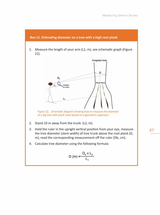
Measuring Carbon Stocks
67
Box 11. Es ma ng diameter on a tree with a high root plank
Measure the length of your arm (L1, m), see schema c graph (Figure 1. 22).
Stand 10 m away from the trunk (L2, m).2.
Hold the ruler in the upright ver cal posi on from your eye, measure 3. the tree diameter (stem width) of tree trunk above the root plank (D, m), read the corresponding measurement off the ruler (Db, cm).
Calculate tree diameter using the following formula: 4.
Schema c diagram showing how to measure the diameter Figure 22. of a big tree with plank roots based on a geometric approach.

Measuring Carbon Stocks
68
2.7.2.3. How to convert tree measurement data to aboveground biomass
Forest inventories are most useful to evaluate the magnitude of carbon fluxes between aboveground forest ecosystems and the atmosphere. Guidelines have been published for establishing permanent plots, characterizing trees correctly and for es ma ng aboveground biomass (Brown, 1997; Gibbs et al., 2007). Tree biomass can be es mated using allometric equa on for specific tree species. Tree allometry establishes quan ta ve rela ons between some key characteris c dimensions of the tree which are usually fairly easy to measure (such as tree diameter and height) and other proper es that are o en more difficult to assess (biomass). However one of the largest sources of uncertainty is the lack of standard models using allometric equa ons to convert tree measurements to aboveground biomass. This has resulted mainly because of the very large diversity of trees species and variety of tree ages (related to diameter) growing in a tropical forest, so it is not possible to use only one specific regression model as can o en be done in the temperate zone (Brown, 1997). Furthermore, direct tree harvest data (especially from big trees) are very limited, so it is impossible to independently assess the model’s quality.
Allometric equa ons can be locally developed by destruc ve sampling, or derived from the literature for supposedly comparable forest types. The equa ons developed by Brown (1997) are based on diameter (D) at breast height (1.3 m) and the height of the tree (H) and have been used widely in the tropics. Separate equa ons have been developed for tropical forests in different annual rainfall regimes: dry < 1500mm; moist 1500-4000mm; and wet > 4000mm. For the humid tropics, however, using the generic allometric equa on developed by Brown (1997) resulted in an overes mate (double the correct amount). Using tree-specific allometrics that include es mates of wood density lead to lower biomass es mates, especially in the low-to-medium biomasss categories (van Noordwijk et al., 2002). A cri cal reassessment of the quality of models across tropical forests and agroforestry types performed by Chave et al. (2005) suggested that the most important predictors of aboveground biomass (AGB) of a tree were, in decreasing order of importance, its trunk diameter, wood specific gravity, total height and forest type (dry, moist or wet). Separate equa ons that have been developed for tropical forests and agroforestry are presented in Table 2, while the es ma on of the biomass of trees which have been regularly pruned or trees from monoco le families such as the coconut tree and oil palm are presented in Table 3.

Measuring Carbon Stocks
69
Life zone (rainfall, mm/yr)
Allometric Equa on
Dry (<1500) (AGB)1. est = 0.112 (rD2H)0.916
(AGB)2. est = ρ * exp(-0.667+1.784 ln(D)+0.207 (ln(D))2 – 0.0281 (ln(D))3)
Humid/ moist
(1500–4000)
(AGB)1. est = 0.0509 x ρD2H
(AGB)2. est = ρ * exp(-1.499+2.148 ln(D)+0.207 (ln(D))2 – 0.0281 (ln(D))3 )
Wet (>4000) (AGB)1. est = 0.0776 * (ρD2H)0.94
(AGB)2. est = ρ * exp(-1.239 + 1.980 ln(D)+0.207 (ln(D))2– 0.0281 (ln(D))3)
Note: (AGB)est = Es mated aboveground tree biomass, kg/tree; D = DBH, diameter at breast height, cm; H = tree height, m; r = Wood density, g cm-3, ρ = Wood specific gravity, Mg m-3. (available from: h p://www.worldagroforestry.org/sea/Products/AFDbases/AF/index.asp).
Model Validity
These regression models are valid only for broadleaf trees with stem diameters in the • range 5–156 cm and tree biomass in the range 50 g – 1 t.
These equa ons should NOT be used beyond their range of validity. Es ma on of • the biomass of conifer tree species, palms, lianas, and the bamboo family should use separately established equa ons.
Allometric equa on for es ma ng biomass (kg per tree) from tree diameter 5–60 cm Table 2. of different life zones (Chave et al., 2005).

Measuring Carbon Stocks
70
Tree species Allometric equa on Source
Coffee regularly pruned
(AGB)est = 0.281 D2.06 Arifin, 2001
Cacao (AGB)est = 0.1208 D1.98 Yuliasmara, 2008
Oil palm (AGB)est = 0.0976 H + 0.0706 ICRAF, 2009
Palm(AGB)est = exp{-2.134 + 2.530 x ln(D)} Brown, 1997
(AGB)est = 4.5 + 7.7 x HFrangi and Lugo, 1985
Bamboo (AGB)est = 0.131 D2.28 Priyadarsini, 2000
Banana (AGB)est = 0.030 D2.13 Arifin, 2001
Note: (AGB)est = Es mated aboveground tree biomass, kg/tree; D = DBH, diameter at breast height, cm; H = tree height, m; r = Wood density, gcm-3,ρ = Wood specific gravity, Mg m-3. (available from: h p://www.worldagroforestry.org/sea/Products/AFDbases/AF/index.
asp).
Box 12. Regression models for es ma ng aboveground tree biomass
Trees hold large stores of C, but great uncertainty remains regarding their quan ta ve contribu on to the global C cycle. Regression models are used to es mate the aboveground tree biomass (ABG) grown in a natural forest or in agroforestry system, such as developed by Ke erings et al. (2001):
Y = a ρ Db
Where: a = intercept Y; b= power coefficient; ρ = wood specific gravity (g cm-3); D = diameter at breast height DBH (cm).
Analysis using data from various allometric equa ons developed by Waterloo (1995), Siregar and Dharmawan (2000), Ke erings et al. (2001), Zianis and Mencuccini (2004) Chave et al. (2005) and Santos (2005) shows that the above allometric equa on has one, rather than two
Allometric equa ons for es ma ng biomass (kg per tree) from trees with regular Table 3. pruning (coffee and cacao) and trees from monoco le families such as palm trees (coconut and oil palm) and bamboo as well as other crops (banana).

Measuring Carbon Stocks
71
Con nued...
degrees of freedom, as the a and the b parameters are strongly linked (Figure 23).
When the empirical linkage between the a and b parameters is used (Figure 23), the different equa ons show a minimal difference for a tree diameter of approximately 30 cm; equa ons with a low power coefficient yield rela vely high biomass es mates in the lower diameter range, but rela vely low ones in the higher diameter range, and vice versa. If the equa ons are applied to a forest stand, rather than a tree, the results have a low dependence on the specific allometric equa on chosen if the majority of tree diameters are < 30 cm but some reach up to 50 or 60 cm. Only if trees > 60 cm diameter are present will the choice of equa on have a substan al effect. Unfortunately, site-specific allometric equa ons for the local forest giants can only be secured by destruc ve sampling of all the big trees – in which case the data will refer to natural history and not current reality. Some uncertainty in the final es mate must be accepted.
Empirical rela onship Figure 23. between a (intercept) and b (power coefficient) of published allometric rela ons of aboveground tree biomass, a er correc ng the a parameter for wood specific gravity (ρ).
Rela onship between Figure 24. stem diameter and tree biomass for allometric rela ons for different b parameters, in which the a and b parameters are linked as indicated in Figure 23.

Measuring Carbon Stocks
72
2.7.2.4 Es ma ng tree root biomass
Large trees tend to have large roots which are an important part of the C cycle because they transfer large amounts of C directly into soil where it may be stored for a long me. For rapid appraisals use default ra os appropriate for the clima c zone, as discussed before. If these assump ons need to be verified, allometric equa ons based on proximal root diamaters need to be developed (van Noordwijk and Mulia, 2002).
2.7.3. Measuring Carbon at plot level
In forest and agricultural ecosystems, C is mainly stored in the plant biomass (aboveground and belowground) and in the soil. The aboveground biomass comprises all woody stems, branches and leaves of living trees, creepers, climbers and epiphytes as well as understory plants and herbaceous undergrowth (see Photo 7). For agricultural land, this includes crops and weed biomass. The dead organic ma er pool (necromass) includes dead fallen trees, other coarse woody debris, li er and charcoal (or par ally charred organic ma er) above the soil surface. The carbon stock of li erfall in a tropical rain forest is typically about 10 Mg ha-1 yr-1, with a mean residence
me in the li er layer of about 1 year. Dead trees may take about 10 years to decompose, and the necromass is about 10% of total aboveground carbon stock in a healthy natural forest. Logging tends to focus on the more valuable trees, damaging many others. A er logging, the necromass may be 30–40% of the aboveground carbon stock. If fire is used in land clearing, the C in this necromass will be emi ed to the atmosphere, otherwise it may take a decade to decay.
Some measurements of the three pools of carbon stock at the plot level are described in Table 4, which are the same as described in the IPCC guidelines (IPCC, 2006) and consist of three steps:
Assessment of biomass. The biomass measured includes trees and • understory (herbaceous) biomass. Aboveground biomass can be measured destruc vely for annual crops or grasses or for the understory. Tree biomass can be measured non-destruc vely using allometric biomass

Measuring Carbon Stocks
73
regression equa ons as described in sec on 2.7.2. Below-ground biomass (roots) can be es mated using a default value (Chave et al., 2007).
Assessment of necromass. Destruc ve assessment is possible for li er • remaining on the soil surface or the assessment can be non-destruc ve for dead wood.
Assessment of soil organic ma er. Determina on of this source of C has to • be carried out in the laboratory.
Measurement Method
Biomass
Aboveground • biomass of living trees
Non-destruc ve, apply allometric equa on
Understory/• herbaceous
Destruc ve
Belowground • biomass (roots)
Non-destruc ve, using default value (Cairns et al., 1997; Mokany et al., 2006)
Necromass
Dead standing trees• Non-destruc ve, apply equa on for volume of cylinder (for branched and unbranched remains)
Dead felled trees• Non-destruc ve, apply equa on for volume of cylinder (or allometric equa on)
Stump (trunk) • remains on forest
Non-destruc ve, apply equa on for volume of cylinder
Li er (coarse/• standing li er, fine li er, surface roots
Destruc ve sampling
Soil Organic Ma erDestruc ve sampling followed by laboratory analysis
Aboveground measurements and methods used in C stock measurement.Table 4.

Measuring Carbon Stocks
74
Carbon stored in living biomass comprises all tree biomass and understory plants in Photo 7. a forest ecosystem (1 and 2) and in biomass and herbaceous undergrowth in an agroforestry system (3 and 4). The dead organic ma er pool (necromass) includes dead fallen trees, other coarse burned wood and woody debris, li er and charcoal (5–8).
Related Documents