Measuring and Modelling Snow Cover and Melt in ... - HimalDoc

i

ICIMOD Working Paper 2016/10

Measuring and Modelling Snow Cover and Melt in a Himalayan Catchment Instrumentation and model code setup in the Langtang catchment, Nepal

Lessons learned from the SnowAMP project

ii

ICIMOD gratefully acknowledges the support of its core donors: The Governments of Afghanistan, Australia, Austria, Bangladesh, Bhutan, China, India, Myanmar, Nepal, Norway, Pakistan, Switzerland, and the United Kingdom.

About ICIMOD

The International Centre for Integrated Mountain Development (ICIMOD) is a regional knowledge

development and learning centre serving the eight regional member countries of the Hindu Kush

Himalayas (HKH) – Afghanistan, Bangladesh, Bhutan, China, India, Myanmar, Nepal, and Pakistan

– based in Kathmandu, Nepal. Globalization and climate change are having an increasing

influence on the stability of fragile mountain ecosystems and the livelihoods of mountain people.

ICIMOD aims to assist mountain people to understand these changes, adapt to them, and make the

most of new opportunities, while addressing upstream and downstream issues. ICIMOD supports

regional transboundary programmes through partnerships with regional partner institutions,

facilitates the exchange of experiences, and serves as a regional knowledge hub. It strengthens

networking among regional and global centres of excellence. Overall, ICIMOD is working to

develop economically- and environmentally-sound mountain ecosystems to improve the living

standards of mountain populations and to sustain vital ecosystem services for the billions of people

living downstream – now and in the future.

International Centre for Integrated Mountain Development Kathmandu, Nepal, December 2016

Authors

Tuomo Saloranta1

Maxime Litt2

Kjetil Melvold1

Measuring and Modelling Snow Cover and Melt in a Himalayan Catchment Instrumentation and model code setup in the Langtang catchment, Nepal. Lessons learned from the SnowAMP project

ICIMOD Working Paper 2016/10

1 Norwegian Water Resources and Energy Directorate (NVE)2 International Centre for Integrated Mountain Development (ICIMOD)

Published byInternational Centre for Integrated Mountain Development GPO Box 3226, Kathmandu, Nepal

Copyright © 2016

International Centre for Integrated Mountain Development (ICIMOD)

All rights reserved. Published 2016

ISBN 978 92 9115 429 6 (printed)

978 92 9115 430 2 (electronic)

Author affiliation

Rucha Ghate, Senior Governance and NRM Specialist, ICIMODRohini Chaturvedi, Consultant, ICIMOD

Production team

Beatrice Murray (Consultant editor)Amy Sellmyer (Editor)Punam Pradhan (Graphic designer)Asha Kaji Thaku (Editorial assistant)

Photos: Kjetil Melvold – pp 8, 9; Maxime Litt – pp iv, 4, 8, 10, 12, 13, 14

Cover: View toward Ganja La pass northern slopes from tserko-ri slopes, as viewed by an automatic timelapse camera, after a snow event in March 2016

Printed and bound in Nepal by

Hill Side (P) Ltd., Kathmandu, Nepal

Note

This publication may be reproduced in whole or in part and in any form for educational or non-profit purposes without special permission from the copyright holder, provided acknowledgement of the source is made. ICIMOD would appreciate receiving a copy of any publication that uses this publication as a source. No use of this publication may be made for resale or for any other commercial purpose whatsoever without prior permission in writing from ICIMOD.

The views and interpretations in this publication are those of the author(s). They are not attributable to ICIMOD and do not imply the expression of any opinion concerning the legal status of any country, territory, city or area of its authorities, or concerning the delimitation of its frontiers or boundaries, or the endorsement of any product.

This publication is available in electronic form at www.icimod.org/himaldoc

Citation: Saloranta, T; Litt, M; Melvold, K (2016) Measuring and modelling snow cover and melt in a Himalayan catchment. Instrumentation and model code setup in the Langtang catchment, Nepal. Lessons learned from the SnowAMP project. ICIMOD Working Paper 2016/10 Kathmandu: ICIMOD

Contents

Summary iv

Acknowledgements v

Acronyms and Abbreviations v

Introduction 1

Role of Seasonal Snow Cover in the Himalayan Region 1

Snow Observations and Modelling 1

The SnowAMP Project 2

Snow Observations 5

Description of the Sites and Stations 5

The Field Campaigns 10

Modelling Methods 15

The seNorge Snow Model Code 15

Summary and Further Research 25

References 26

iv

Summary

Seasonal snow cover plays an important role in water resources availability in many regions of the world and is a key factor in the weather and climate system, both regionally and globally. Snowmelt can be a source of water for human use, such as irrigation and hydropower production, but can also cause disasters such as floods and slush avalanches. Reliable models must be developed to accurately simulate snow cover and melt, and to obtain reliable forecasts of snow impact on risks and current downstream water availability, and their likely evolution in the context of climate change. In the Hindu Kush Himalayas (HKH), little is known about snow cover and snowmelt processes as in situ measurements are challenging to undertake in remote, high altitude sites. Snow conditions vary strongly with the time of year, region, elevation, and between years depending on the prevailing weather type. In situ data are needed to improve models and increase our understanding of snow accumulation and melt processes.

To address this, the International Centre for Integrated Mountain Development (ICIMOD) and the Norwegian Water Resources and Energy Directorate (NVE) have developed a project on ‘Snow accumulation and melt processes in a Himalayan catchment (SnowAMP)’ with a four-year time frame from 2014 to 2017. The SnowAMP project is intended to increase scientific knowledge on snowmelt and accumulation dynamics and the role of snowmelt in water resources in the Hindu Kush Himalayan watersheds. The aim is to install automatic weather stations dedicated to snow monitoring in a Himalayan catchment and use the data from these to develop a snow model and evaluate it in the catchment. The final objective is to use data from ground-based weather and snow measurements, together with data from satellite images and other sources, in combination with the model in order to provide useful, near real-time estimates of the amount of snow in a catchment, and to increase understanding of the contribution of snowmelt to river runoff. Three local partners are also involved – Kathmandu University (KU), Tribhuvan University (TU), and the Department of Hydrology and Meteorology (DHM). The Langtang catchment in Rasuwa district, Nepal, was chosen as the site for in situ snow monitoring. A model was developed using the open source ‘R’ statistical software.

This publication presents the mid-term results of the project and is aimed especially at those planning similar research projects. It highlights the challenges of in situ snow monitoring in the Himalayas, reports the issues encountered and lessons learned during installation of the automatic field stations, and proposes a method for snowmelt modelling. It starts with a description of the snow conditions in the HKH and the state-of-the-art knowledge on snow measurements; describes the technical details of the setup of snow and weather instrumentation and the issues faced during installation; and discusses analysis and modelling techniques, the challenges of their application in the HKH mountain environment, and details of the model developed for the Langtang catchment.

v

Acknowledgements

NVE and ICMOD thank all the partners from Kathmandu University, Tribhuvan University, and the Department of Hydrology and Meteorology in Nepal for their contribution to this project. Special thanks are addressed to all the participants for the successful field campaigns and good co-operation in Langtang valley in 2015/16, and to ICIMOD’s internal reviewers, Anna Sinisalo, Joseph Shea, and Inka Koch, who contributed to the final version of this document.

Acronyms and Abbreviations

HKH Hindu Kush Karakoram Himalayan NVE Norwegian Water Resources and Energy Directorate SCA snow-covered area SD snow depthSWE snow water equivalent

vi

1

Introduction

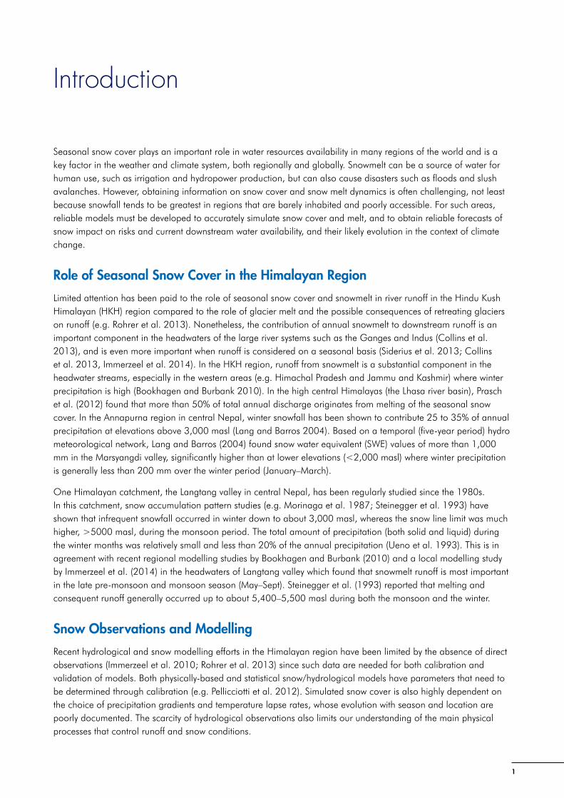
Seasonal snow cover plays an important role in water resources availability in many regions of the world and is a key factor in the weather and climate system, both regionally and globally. Snowmelt can be a source of water for human use, such as irrigation and hydropower production, but can also cause disasters such as floods and slush avalanches. However, obtaining information on snow cover and snow melt dynamics is often challenging, not least because snowfall tends to be greatest in regions that are barely inhabited and poorly accessible. For such areas, reliable models must be developed to accurately simulate snow cover and melt, and to obtain reliable forecasts of snow impact on risks and current downstream water availability, and their likely evolution in the context of climate change.

Role of Seasonal Snow Cover in the Himalayan Region

Limited attention has been paid to the role of seasonal snow cover and snowmelt in river runoff in the Hindu Kush Himalayan (HKH) region compared to the role of glacier melt and the possible consequences of retreating glaciers on runoff (e.g. Rohrer et al. 2013). Nonetheless, the contribution of annual snowmelt to downstream runoff is an important component in the headwaters of the large river systems such as the Ganges and Indus (Collins et al. 2013), and is even more important when runoff is considered on a seasonal basis (Siderius et al. 2013; Collins et al. 2013, Immerzeel et al. 2014). In the HKH region, runoff from snowmelt is a substantial component in the headwater streams, especially in the western areas (e.g. Himachal Pradesh and Jammu and Kashmir) where winter precipitation is high (Bookhagen and Burbank 2010). In the high central Himalayas (the Lhasa river basin), Prasch et al. (2012) found that more than 50% of total annual discharge originates from melting of the seasonal snow cover. In the Annapurna region in central Nepal, winter snowfall has been shown to contribute 25 to 35% of annual precipitation at elevations above 3,000 masl (Lang and Barros 2004). Based on a temporal (five-year period) hydro meteorological network, Lang and Barros (2004) found snow water equivalent (SWE) values of more than 1,000 mm in the Marsyangdi valley, significantly higher than at lower elevations (<2,000 masl) where winter precipitation is generally less than 200 mm over the winter period (January–March).

One Himalayan catchment, the Langtang valley in central Nepal, has been regularly studied since the 1980s. In this catchment, snow accumulation pattern studies (e.g. Morinaga et al. 1987; Steinegger et al. 1993) have shown that infrequent snowfall occurred in winter down to about 3,000 masl, whereas the snow line limit was much higher, >5000 masl, during the monsoon period. The total amount of precipitation (both solid and liquid) during the winter months was relatively small and less than 20% of the annual precipitation (Ueno et al. 1993). This is in agreement with recent regional modelling studies by Bookhagen and Burbank (2010) and a local modelling study by Immerzeel et al. (2014) in the headwaters of Langtang valley which found that snowmelt runoff is most important in the late pre-monsoon and monsoon season (May–Sept). Steinegger et al. (1993) reported that melting and consequent runoff generally occurred up to about 5,400–5,500 masl during both the monsoon and the winter.

Snow Observations and Modelling

Recent hydrological and snow modelling efforts in the Himalayan region have been limited by the absence of direct observations (Immerzeel et al. 2010; Rohrer et al. 2013) since such data are needed for both calibration and validation of models. Both physically-based and statistical snow/hydrological models have parameters that need to be determined through calibration (e.g. Pellicciotti et al. 2012). Simulated snow cover is also highly dependent on the choice of precipitation gradients and temperature lapse rates, whose evolution with season and location are poorly documented. The scarcity of hydrological observations also limits our understanding of the main physical processes that control runoff and snow conditions.

2

Snow conditions in mountainous regions vary strongly with the time of year, region, and elevation, as well as between years, depending on the prevailing weather type. In more accessible areas, these changes can be recorded through direct observation, but in remote mountainous regions, direct observations of snowfall and snowmelt are sparse, and it is not possible to use observational data to accurately map the snow cover and melt distribution. In Norway, for example, most snow observations consist of ground-based point observations of snow depth (SD) which are combined with satellite-based images of the fraction of snow-covered area (SCA), whereas in the Himalayas, the ground-based snow monitoring network is very sparse and satellite images of SCA are usually the only information available. In areas with few direct observations, mapping can be obtained from accurate models that rely on a limited amount of input data and are able to account for the observed spatial and temporal variability. But such models rely on a strong knowledge of physical snow processes and must be validated initially against in-situ data to ensure they consistently account for the wide range of snow dynamics under a wide range of conditions.

While knowledge of the current SCA and snowmelt rates are normally sufficient for assessing the regional short-term (e.g. 1–3 days) meltwater runoff from a snow pack warmed to 0ºC and ready to melt, the decrease of SCA during the snowmelt season is strongly dependent on the spatial distribution of snow water equivalent (SWE), i.e. how much water is stored in the snow pack. SWE can be derived from the snow depth (SD) and the bulk density of the snow pack ρ as SWE = SD.ρ. Good knowledge of SWE is crucial for assessing the longer-term (>3 days) snowmelt water contribution to discharge. Former studies have used SCA data to estimate SWE or snowmelt runoff, as they are closely related (Duethmann et al. 2014; Kolberg et al. 2006; Kolberg and Gottschalk, 2010; Parajka and Blöschl, 2008; Pellicciotti et al. 2012). But the performance of models using SCA data to estimate SWE appears to be model dependent. For example, SCA observations alone were able to increase the discharge model performance in Kolberg and Gottschalk (2010), especially if images from several dates during the snowmelt season were assimilated, while Pellicciotti et al. (2012) indicated that satellite-based SCA observations did not contain sufficient information alone to properly calibrate the snow mass balance in their hydrological models.

Several different hydrological and snow models have been applied in the Langtang catchment. Braun et al. (1993) applied the HBV3-ETH hydrological rainfall-runoff model to simulate water balance in the catchment. Pradhananga et al. (2014) simulated the present and future discharge of the Langtang river using a glacio-hydrological model which used the positive-degree day approach to calculate snow and glacier melt at different elevation zones. Immerzeel et al. (2012, 2013) applied a high-resolution combined cryospheric hydrological model to the Langtang catchment using the PCRaster environment for numerical modelling. Recently, they also applied the TOPKAPI-ETH model to demonstrate the impact of uncertain vertical air temperature and precipitation gradients on model results (Immerzeel et al. 2014).

In Norway, national snow maps have been produced using the seNorge snow model since 2004 to provide detailed information on regional snow conditions (Saloranta 2012; 2014a,b; 2016). This service is a co-operation between the Norwegian Water Resources and Energy Directorate (NVE) and the Norwegian Meteorological Institute (MET). The seNorge snow model simulates different snow-related variables, such as SWE, SD, SCA, ρ, and the amount of liquid water in the snowpack (WL). In Norway the model is applied to produce snow maps with 1x1 km resolution, and runs daily in a grid of approximately 324,000 cells. The resulting snow maps are used, for example, to compose weekly reports on snow conditions for hydropower production and power system planning, as well as for forecasting of runoff, floods, and the risk of avalanches. These reports also inform the public about skiing conditions, and are used in scientific studies.

The SnowAMP Project

Based on the work in Norway, the International Centre for Integrated Mountain Development (ICIMOD) and the Norwegian Water Resources and Energy Directorate (NVE) have developed a project on ‘Snow accumulation and melt processes in a Himalayan catchment’ (SnowAMP)’ to increase scientific knowledge on snowmelt and accumulation dynamics and the role of snowmelt in water resources in the Hindu Kush Himalayan watersheds. The immediate aim is to help fill the gap in the in-situ snow measurements needed to calibrate and validate models for calculating snow parameters in the Himalayas.

3

The project has a four-year time frame from 2014 to 2017. Three local partner institutes are involved – Kathmandu University (KU), Tribhuvan University (TU), and the Department of Hydrology and Meteorology (DHM). A network of four automatic weather stations dedicated to snow monitoring has been installed in the Langtang catchment in Rasuwa district, Nepal, to provide data that can be used to develop and evaluate a snow model for the catchment based on the seNorge model. The final objective is to use data from ground-based weather and snow measurements, together with data from satellite images and other sources, in combination with the model in order to provide useful, near real-time estimates of the amount of snow in a Himalayan catchment, and to increase understanding of the contribution of snowmelt water to river runoff.

The first part of the report describes the site, instruments, and measured variables, as well as the issues encountered during the station installation and maintenance. The second part focuses on a description of the seNorge model in the version adapted for use in the Langtang catchment. The aim is to provide tips and advice for future research and in-situ snow monitoring experiments in the region.

4

5

Snow Observations

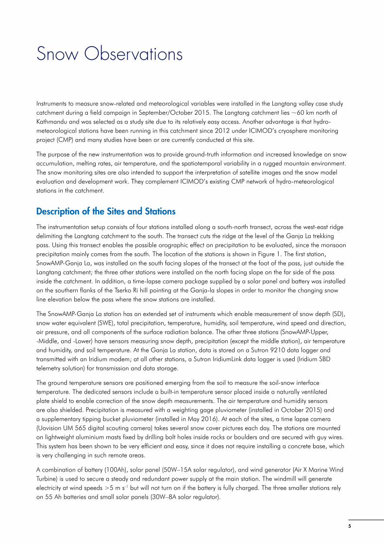
Instruments to measure snow-related and meteorological variables were installed in the Langtang valley case study catchment during a field campaign in September/October 2015. The Langtang catchment lies ~60 km north of Kathmandu and was selected as a study site due to its relatively easy access. Another advantage is that hydro-meteorological stations have been running in this catchment since 2012 under ICIMOD’s cryosphere monitoring project (CMP) and many studies have been or are currently conducted at this site.

The purpose of the new instrumentation was to provide ground-truth information and increased knowledge on snow accumulation, melting rates, air temperature, and the spatiotemporal variability in a rugged mountain environment. The snow monitoring sites are also intended to support the interpretation of satellite images and the snow model evaluation and development work. They complement ICIMOD’s existing CMP network of hydro-meteorological stations in the catchment.

Description of the Sites and Stations

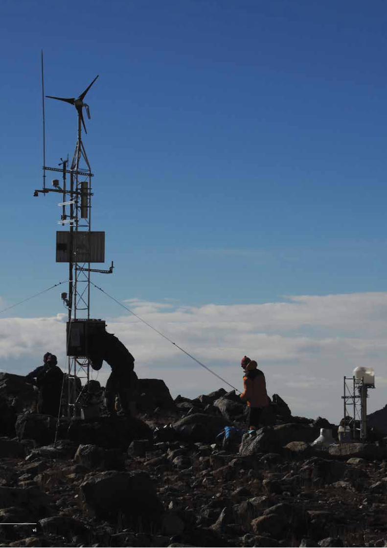
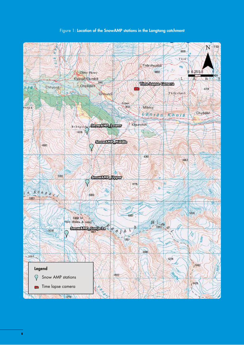
The instrumentation setup consists of four stations installed along a south-north transect, across the west-east ridge delimiting the Langtang catchment to the south. The transect cuts the ridge at the level of the Ganja La trekking pass. Using this transect enables the possible orographic effect on precipitation to be evaluated, since the monsoon precipitation mainly comes from the south. The location of the stations is shown in Figure 1. The first station, SnowAMP-Ganja La, was installed on the south facing slopes of the transect at the foot of the pass, just outside the Langtang catchment; the three other stations were installed on the north facing slope on the far side of the pass inside the catchment. In addition, a time-lapse camera package supplied by a solar panel and battery was installed on the southern flanks of the Tserko Ri hill pointing at the Ganja-la slopes in order to monitor the changing snow line elevation below the pass where the snow stations are installed.

The SnowAMP-Ganja La station has an extended set of instruments which enable measurement of snow depth (SD), snow water equivalent (SWE), total precipitation, temperature, humidity, soil temperature, wind speed and direction, air pressure, and all components of the surface radiation balance. The other three stations (SnowAMP-Upper, -Middle, and -Lower) have sensors measuring snow depth, precipitation (except the middle station), air temperature and humidity, and soil temperature. At the Ganja La station, data is stored on a Sutron 9210 data logger and transmitted with an Iridium modem; at all other stations, a Sutron IridiumLink data logger is used (Iridium SBD telemetry solution) for transmission and data storage.

The ground temperature sensors are positioned emerging from the soil to measure the soil-snow interface temperature. The dedicated sensors include a built-in temperature sensor placed inside a naturally ventilated plate shield to enable correction of the snow depth measurements. The air temperature and humidity sensors are also shielded. Precipitation is measured with a weighting gage pluviometer (installed in October 2015) and a supplementary tipping bucket pluviometer (installed in May 2016). At each of the sites, a time lapse camera (Uovision UM 565 digital scouting camera) takes several snow cover pictures each day. The stations are mounted on lightweight aluminium masts fixed by drilling bolt holes inside rocks or boulders and are secured with guy wires. This system has been shown to be very efficient and easy, since it does not require installing a concrete base, which is very challenging in such remote areas.

A combination of battery (100Ah), solar panel (50W–15A solar regulator), and wind generator (Air X Marine Wind Turbine) is used to secure a steady and redundant power supply at the main station. The windmill will generate electricity at wind speeds >5 m s-1 but will not turn on if the battery is fully charged. The three smaller stations rely on 55 Ah batteries and small solar panels (30W–8A solar regulator).

66

Figure 1: Location of the SnowAMP stations in the Langtang catchment

Snow AMP stations

Time lapse camera

Legend

7

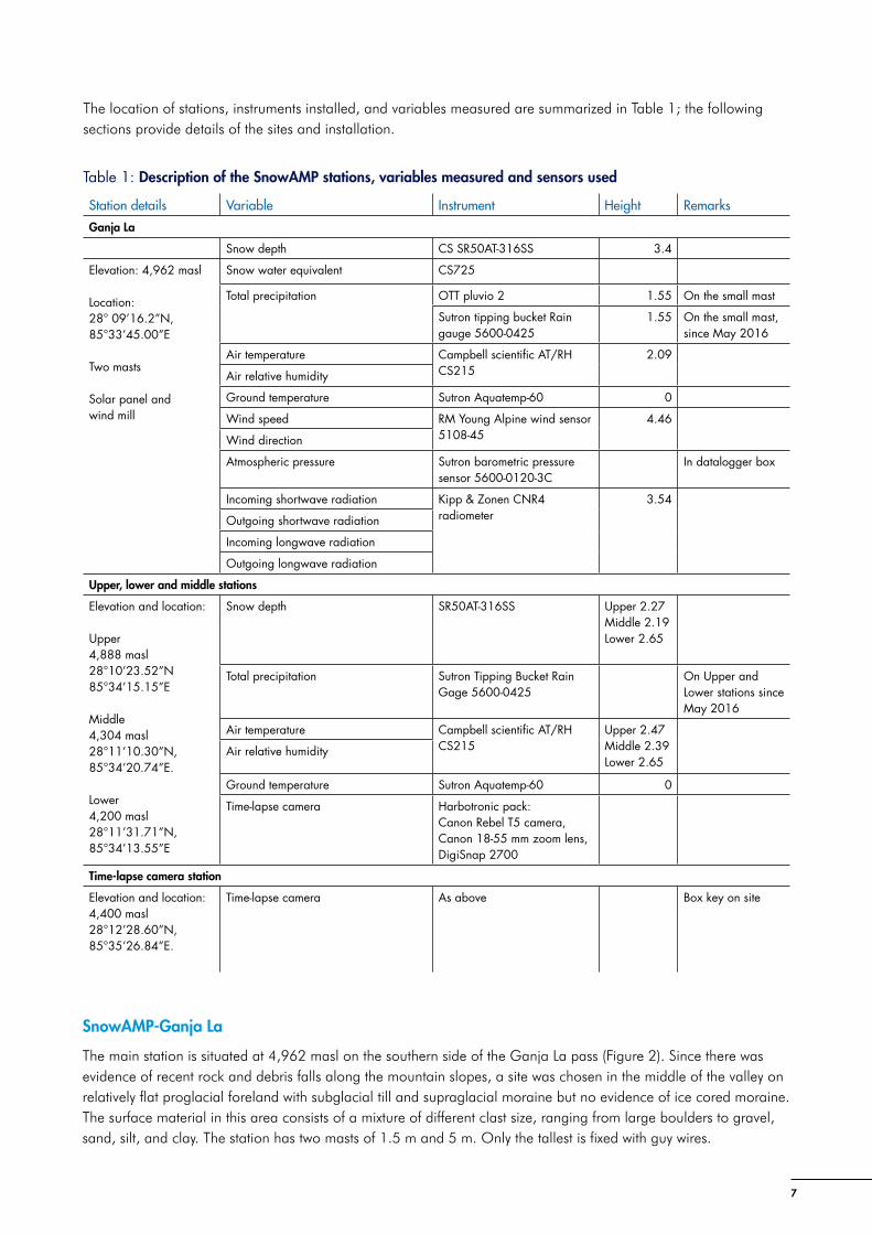
The location of stations, instruments installed, and variables measured are summarized in Table 1; the following sections provide details of the sites and installation.

Station details Variable Instrument Height Remarks

Ganja La

Snow depth CS SR50AT-316SS 3.4

Elevation: 4,962 masl

Location: 28° 09’16.2”N, 85°33’45.00”E

Two masts

Solar panel and wind mill

Snow water equivalent CS725

Total precipitation OTT pluvio 2 1.55 On the small mast

Sutron tipping bucket Rain gauge 5600-0425

1.55 On the small mast, since May 2016

Air temperature Campbell scientific AT/RH CS215

2.09

Air relative humidity

Ground temperature Sutron Aquatemp-60 0

Wind speed RM Young Alpine wind sensor 5108-45

4.46

Wind direction

Atmospheric pressure Sutron barometric pressure sensor 5600-0120-3C

In datalogger box

Incoming shortwave radiation Kipp & Zonen CNR4 radiometer

3.54

Outgoing shortwave radiation

Incoming longwave radiation

Outgoing longwave radiation

Upper, lower and middle stations

Elevation and location: Upper 4,888 masl 28°10’23.52”N 85°34’15.15”E

Middle 4,304 masl 28°11’10.30”N, 85°34’20.74”E.

Lower 4,200 masl 28°11’31.71”N, 85°34’13.55”E

Snow depth SR50AT-316SS Upper 2.27 Middle 2.19 Lower 2.65

Total precipitation Sutron Tipping Bucket Rain Gage 5600-0425

On Upper and Lower stations since May 2016

Air temperature Campbell scientific AT/RH CS215

Upper 2.47Middle 2.39Lower 2.65

Air relative humidity

Ground temperature Sutron Aquatemp-60 0

Time-lapse camera Harbotronic pack: Canon Rebel T5 camera, Canon 18-55 mm zoom lens, DigiSnap 2700

Time-lapse camera station

Elevation and location: 4,400 masl 28°12’28.60”N, 85°35’26.84”E.

Time-lapse camera As above Box key on site

Table 1: Description of the SnowAMP stations, variables measured and sensors used

SnowAMP-Ganja La

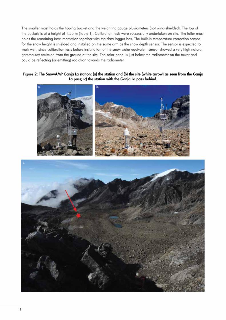
The main station is situated at 4,962 masl on the southern side of the Ganja La pass (Figure 2). Since there was evidence of recent rock and debris falls along the mountain slopes, a site was chosen in the middle of the valley on relatively flat proglacial foreland with subglacial till and supraglacial moraine but no evidence of ice cored moraine. The surface material in this area consists of a mixture of different clast size, ranging from large boulders to gravel, sand, silt, and clay. The station has two masts of 1.5 m and 5 m. Only the tallest is fixed with guy wires.

8

The smaller mast holds the tipping bucket and the weighting gauge pluviometers (not wind-shielded). The top of the buckets is at a height of 1.55 m (Table 1). Calibration tests were successfully undertaken on site. The taller mast holds the remaining instrumentation together with the data logger box. The built-in temperature correction sensor for the snow height is shielded and installed on the same arm as the snow depth sensor. The sensor is expected to work well, since calibration tests before installation of the snow water equivalent sensor showed a very high natural gamma-ray emission from the ground at the site. The solar panel is just below the radiometer on the tower and could be reflecting (or emitting) radiation towards the radiometer.

Figure 2: The SnowAMP Ganja La station: (a) the station and (b) the site (white arrow) as seen from the Ganja La pass; (c) the station with the Ganja La pass behind.

a.

c.

b.

9

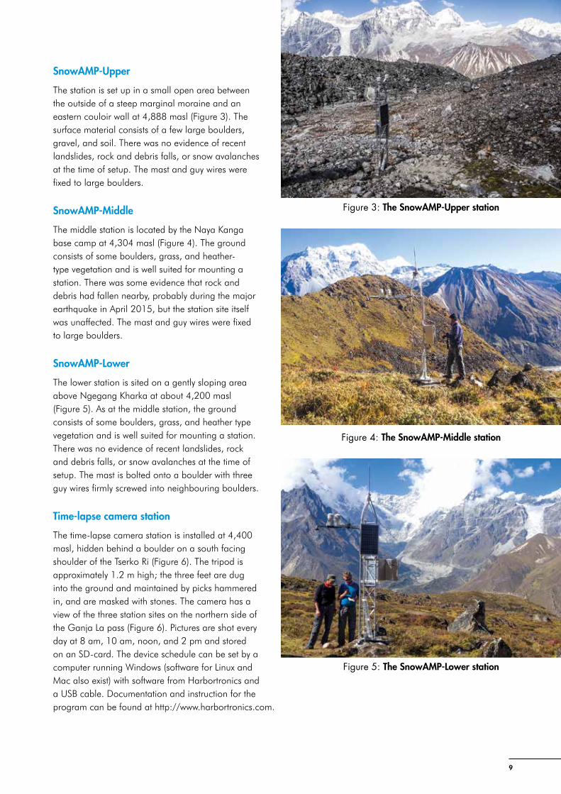
SnowAMP-Upper

The station is set up in a small open area between the outside of a steep marginal moraine and an eastern couloir wall at 4,888 masl (Figure 3). The surface material consists of a few large boulders, gravel, and soil. There was no evidence of recent landslides, rock and debris falls, or snow avalanches at the time of setup. The mast and guy wires were fixed to large boulders.

SnowAMP-Middle

The middle station is located by the Naya Kanga base camp at 4,304 masl (Figure 4). The ground consists of some boulders, grass, and heather-type vegetation and is well suited for mounting a station. There was some evidence that rock and debris had fallen nearby, probably during the major earthquake in April 2015, but the station site itself was unaffected. The mast and guy wires were fixed to large boulders.

SnowAMP-Lower

The lower station is sited on a gently sloping area above Ngegang Kharka at about 4,200 masl (Figure 5). As at the middle station, the ground consists of some boulders, grass, and heather type vegetation and is well suited for mounting a station. There was no evidence of recent landslides, rock and debris falls, or snow avalanches at the time of setup. The mast is bolted onto a boulder with three guy wires firmly screwed into neighbouring boulders.

Time-lapse camera station

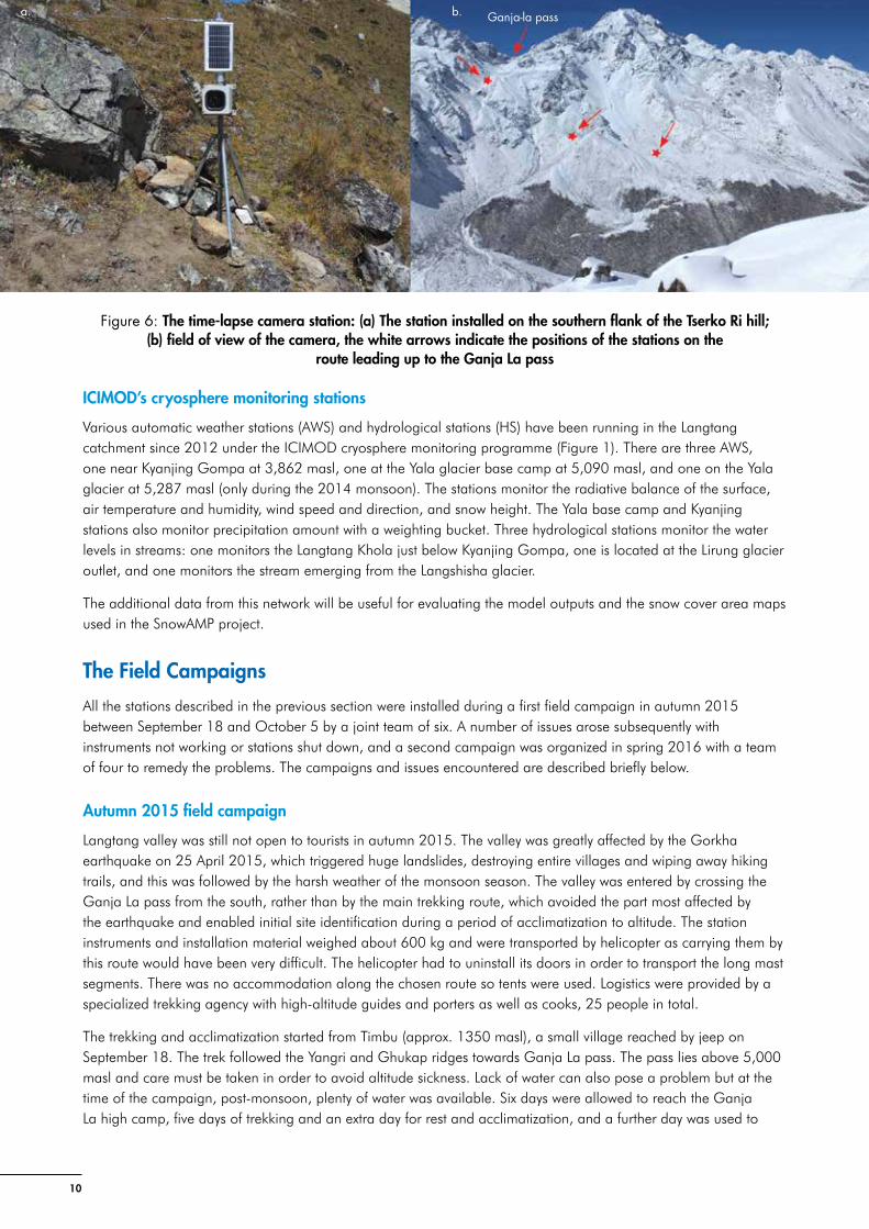
The time-lapse camera station is installed at 4,400 masl, hidden behind a boulder on a south facing shoulder of the Tserko Ri (Figure 6). The tripod is approximately 1.2 m high; the three feet are dug into the ground and maintained by picks hammered in, and are masked with stones. The camera has a view of the three station sites on the northern side of the Ganja La pass (Figure 6). Pictures are shot every day at 8 am, 10 am, noon, and 2 pm and stored on an SD-card. The device schedule can be set by a computer running Windows (software for Linux and Mac also exist) with software from Harbortronics and a USB cable. Documentation and instruction for the program can be found at http://www.harbortronics.com.

Figure 3: The SnowAMP-Upper station

Figure 4: The SnowAMP-Middle station

Figure 5: The SnowAMP-Lower station

10

ICIMOD’s cryosphere monitoring stations

Various automatic weather stations (AWS) and hydrological stations (HS) have been running in the Langtang catchment since 2012 under the ICIMOD cryosphere monitoring programme (Figure 1). There are three AWS, one near Kyanjing Gompa at 3,862 masl, one at the Yala glacier base camp at 5,090 masl, and one on the Yala glacier at 5,287 masl (only during the 2014 monsoon). The stations monitor the radiative balance of the surface, air temperature and humidity, wind speed and direction, and snow height. The Yala base camp and Kyanjing stations also monitor precipitation amount with a weighting bucket. Three hydrological stations monitor the water levels in streams: one monitors the Langtang Khola just below Kyanjing Gompa, one is located at the Lirung glacier outlet, and one monitors the stream emerging from the Langshisha glacier.

The additional data from this network will be useful for evaluating the model outputs and the snow cover area maps used in the SnowAMP project.

The Field Campaigns

All the stations described in the previous section were installed during a first field campaign in autumn 2015 between September 18 and October 5 by a joint team of six. A number of issues arose subsequently with instruments not working or stations shut down, and a second campaign was organized in spring 2016 with a team of four to remedy the problems. The campaigns and issues encountered are described briefly below.

Autumn 2015 field campaign

Langtang valley was still not open to tourists in autumn 2015. The valley was greatly affected by the Gorkha earthquake on 25 April 2015, which triggered huge landslides, destroying entire villages and wiping away hiking trails, and this was followed by the harsh weather of the monsoon season. The valley was entered by crossing the Ganja La pass from the south, rather than by the main trekking route, which avoided the part most affected by the earthquake and enabled initial site identification during a period of acclimatization to altitude. The station instruments and installation material weighed about 600 kg and were transported by helicopter as carrying them by this route would have been very difficult. The helicopter had to uninstall its doors in order to transport the long mast segments. There was no accommodation along the chosen route so tents were used. Logistics were provided by a specialized trekking agency with high-altitude guides and porters as well as cooks, 25 people in total.

The trekking and acclimatization started from Timbu (approx. 1350 masl), a small village reached by jeep on September 18. The trek followed the Yangri and Ghukap ridges towards Ganja La pass. The pass lies above 5,000 masl and care must be taken in order to avoid altitude sickness. Lack of water can also pose a problem but at the time of the campaign, post-monsoon, plenty of water was available. Six days were allowed to reach the Ganja La high camp, five days of trekking and an extra day for rest and acclimatization, and a further day was used to

Figure 6: The time-lapse camera station: (a) The station installed on the southern flank of the Tserko Ri hill; (b) field of view of the camera, the white arrows indicate the positions of the stations on the

route leading up to the Ganja La pass

a. Ganja-la passb.

11

explore potential sites on the way down to Kyanjing Gompa at the bottom of the valley. The helicopters with the equipment were delayed for some days by poor weather, another common problem in isolated mountain areas. During this time, the team were able to study the river discharge measurement stations at Kyanjing and downstream of the Lirung glacier and suggest some improvements. One helicopter brought in all the equipment (in a series of flights) and returned on a second day to transport the equipment from the main camp to the individual sites. The snow stations were installed and tested one by one, starting with the lowest, over a period of four days. Originally more time had been planned, but the delays in helicopter flights reduced the time available. The return trek to Timbu took a further three days and the team returned to Kathmandu on October 5. Two scientists returned to the Ganja La and Upper stations on October 26 to resolve two problems. The snow depth sensor had caused the Upper station to fail and it was not transmitting data. The sensor was replaced, but the station remained inoperative. (For further details, see the spring field campaign below.) There was also a wiring error in the solar panel at the SnowAMP-Ganja La station which was corrected. The incorrect wiring had caused the battery to discharge which had turned off an automatic switch shutting down the SWE sensor, a few hours after installation.

Spring 2016 field campaign

In January 2016, the Lower and Middle stations were working well, but the Upper station was still not functioning and the Ganja La station had not transmitted data since the end of October. A second campaign was organized in the spring to resolve these problems. The team left Kathmandu on 25th of April and trekked from Kakani to Timbu, thereafter following the same route as in autumn, taking five days to reach the Ganja La station, including one day for acclimatization. Work started at the Ganja La station on 30 April, and continued at the other stations over the next days. The issues and actions taken are summarized in the following.

SnowAMP-Ganja La � The station was in a good apparent state with no visible damage and was standing in the same position as

when left in 2015. However, the logger was off with no text and no lights on the modem box inside the main housing, even though the battery and charging status lights were green and the measured voltage on the battery (14.4 V) was normal. No data had been recorded since 31st October 2015. Systematic measurements with a voltmeter revealed that the main fuse had been physically displaced from the fuse-holder and there was no power to the logger. The fuse had probably slipped progressively inside its housing after the maintenance in October 2015. A new fuse was installed correctly and the logger started working again. The fuse-holder was secured with a piece of electric tape to prevent future displacement.

� The new tipping bucket was installed next to the total precipitation gauge (Error! Reference source not found., 8).

� The logger and modem were replaced.

� The consistency of the different sensors measurements was checked. The snow depth sensor showed -0.006 m for bare ground, and -1.6 m when someone was standing below it. No calibration was applied.

� The total precipitation gauge was emptied, levelled, and refilled with five litres of antifreeze.

� The yellow switch on top of the main housing was left unplugged. This switch commands a circuit that controls the shut-down mechanism for the snow water equivalent sensor when power supply is too low. It was left unplugged so that at times of low power, the instruments would continue to run until the battery was discharged.

� CNR4 was tilted and was levelled.

� A new time-lapse camera was installed with new 16GB SD-memory card and 12 AA-lithium batteries and running programme. The switch on the previously installed camera had been left in setup mode and the camera had not captured any images.

� Functioning data transmission was confirmed via satellite phone.

12

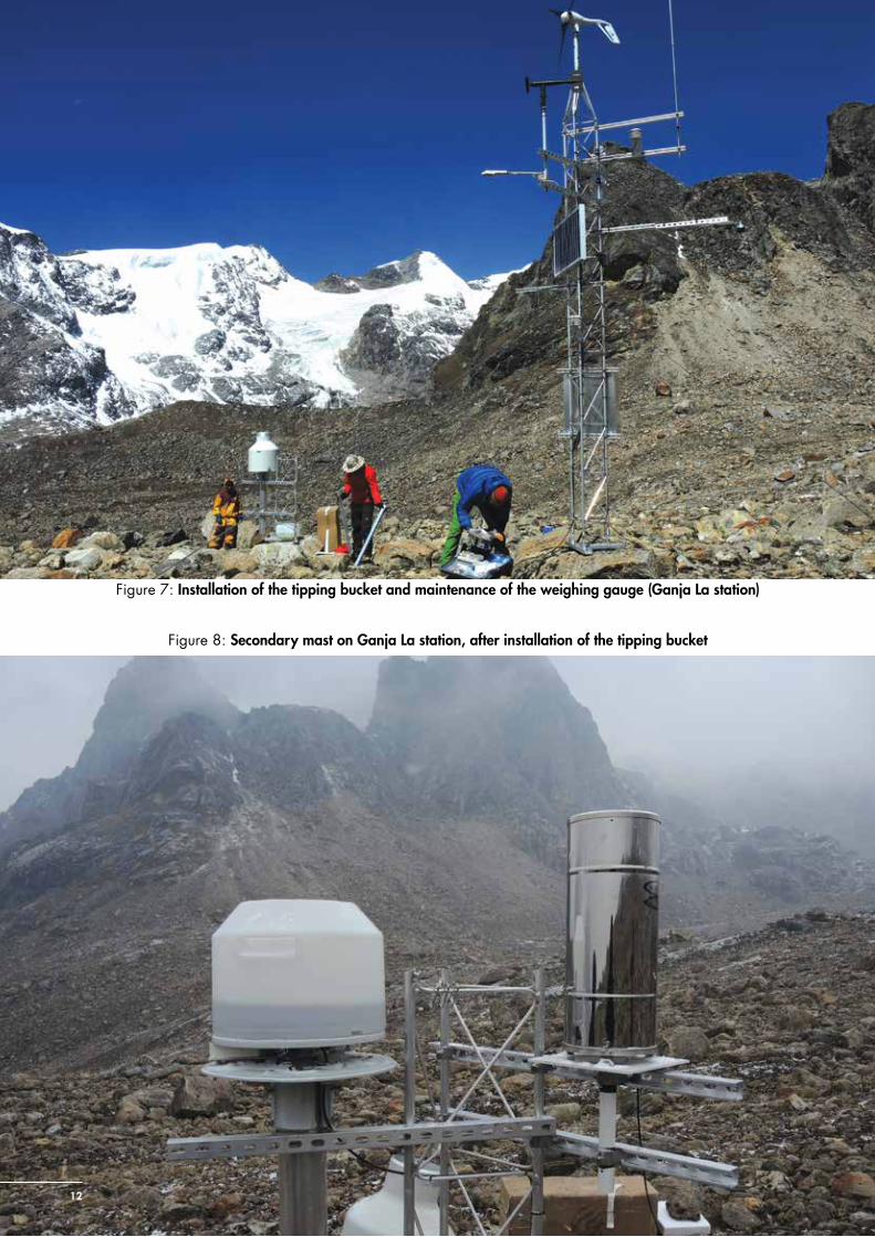
Figure 7: Installation of the tipping bucket and maintenance of the weighing gauge (Ganja La station)

Figure 8: Secondary mast on Ganja La station, after installation of the tipping bucket

13

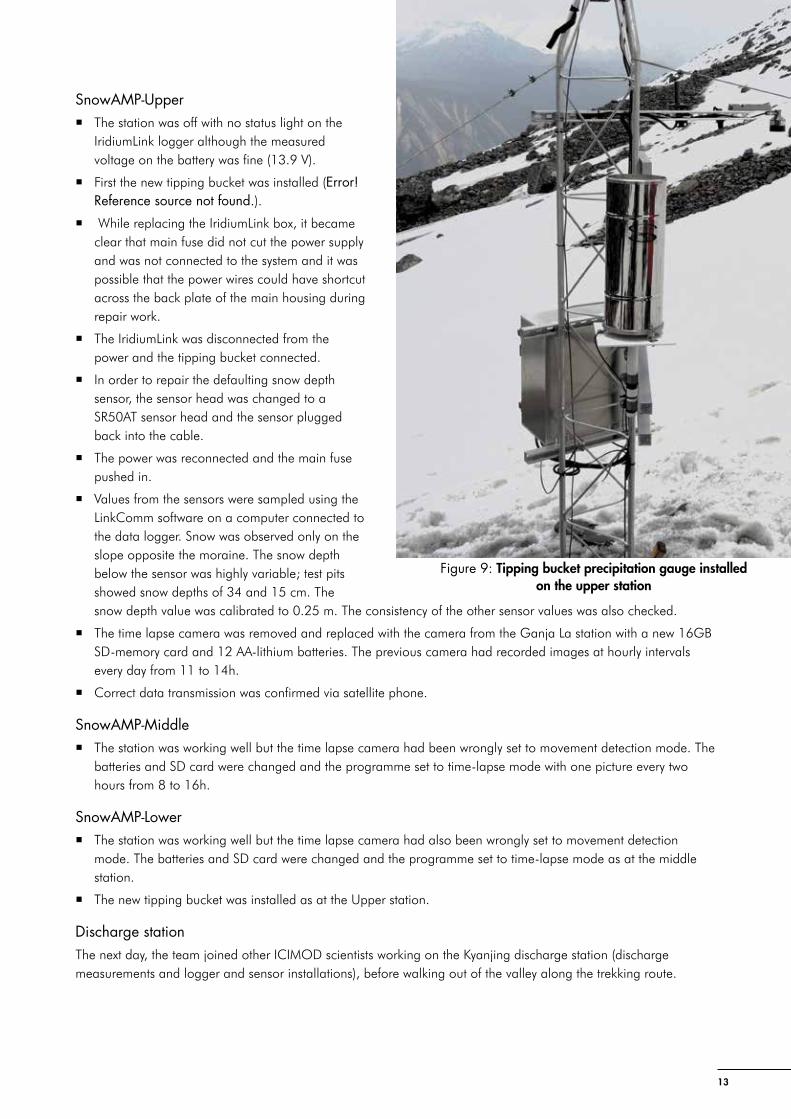
SnowAMP-Upper � The station was off with no status light on the

IridiumLink logger although the measured voltage on the battery was fine (13.9 V).

� First the new tipping bucket was installed (Error! Reference source not found.).

� While replacing the IridiumLink box, it became clear that main fuse did not cut the power supply and was not connected to the system and it was possible that the power wires could have shortcut across the back plate of the main housing during repair work.

� The IridiumLink was disconnected from the power and the tipping bucket connected.

� In order to repair the defaulting snow depth sensor, the sensor head was changed to a SR50AT sensor head and the sensor plugged back into the cable.

� The power was reconnected and the main fuse pushed in.

� Values from the sensors were sampled using the LinkComm software on a computer connected to the data logger. Snow was observed only on the slope opposite the moraine. The snow depth below the sensor was highly variable; test pits showed snow depths of 34 and 15 cm. The snow depth value was calibrated to 0.25 m. The consistency of the other sensor values was also checked.

� The time lapse camera was removed and replaced with the camera from the Ganja La station with a new 16GB SD-memory card and 12 AA-lithium batteries. The previous camera had recorded images at hourly intervals every day from 11 to 14h.

� Correct data transmission was confirmed via satellite phone.

SnowAMP-Middle � The station was working well but the time lapse camera had been wrongly set to movement detection mode. The

batteries and SD card were changed and the programme set to time-lapse mode with one picture every two hours from 8 to 16h.

SnowAMP-Lower � The station was working well but the time lapse camera had also been wrongly set to movement detection

mode. The batteries and SD card were changed and the programme set to time-lapse mode as at the middle station.

� The new tipping bucket was installed as at the Upper station.

Discharge stationThe next day, the team joined other ICIMOD scientists working on the Kyanjing discharge station (discharge measurements and logger and sensor installations), before walking out of the valley along the trekking route.

Figure 9: Tipping bucket precipitation gauge installed on the upper station

14

Time-lapse camera station One week later (May 8) two staff members checked the time lapse camera on Tserko Ri. The station was working well. Data from the SD card was downloaded and the card was reformatted and replaced.

Lessons learned

The installation of snow monitoring stations in the Langtang catchment raised a number of issues which are typical of remote high altitude sites and likely to be encountered in other field campaigns of this type.

� Transportation of heavy equipment is complicated by the difficult access to remote sites, which might favour the use of a helicopter. However, helicopter transportation is very expensive and not necessarily reliable. High altitude flights require calm weather and this can lead to long delays. The helicopter delays and loss of time can mean that stations must be installed faster than desirable. The balance between the costs of flights and of ground transportation, which might be even more expensive although potentially more reliable, has to be weighed up for each situation. Given the uncertainties, the plans should ideally allow for taking extra days if needed, but this also has cost implications.

� Bolting the station masts into rocks instead of building a concrete base stands out as a very convenient solution. It avoids the need to transport cement and other heavy material, and is extremely fast.

� High altitude exposure requires proper acclimatization, so that staff can remain safe and work properly. Safety includes bringing proper safety medical kits and safety material. Note that even with the best acclimatization, people can still get sick.

� The remoteness of the stations impedes regular checks and the possibility of carrying out repairs, thus extra time and care should be taken to ensure that installation is accurate and testing robust.

15

Modelling Methods

The seNorge Snow Model Code

The seNorge snow model was selected for the SnowAMP project (Saloranta 2012; 2014a,b; 2016) as it easily allows data-assimilation procedures, has a fast execution time, and the research team already had experience with it. A further advantage is that the model is coded with the widely used open access software ‘R’. The sources for the model scripts and the software required to run the model (Table 2) are open to all.

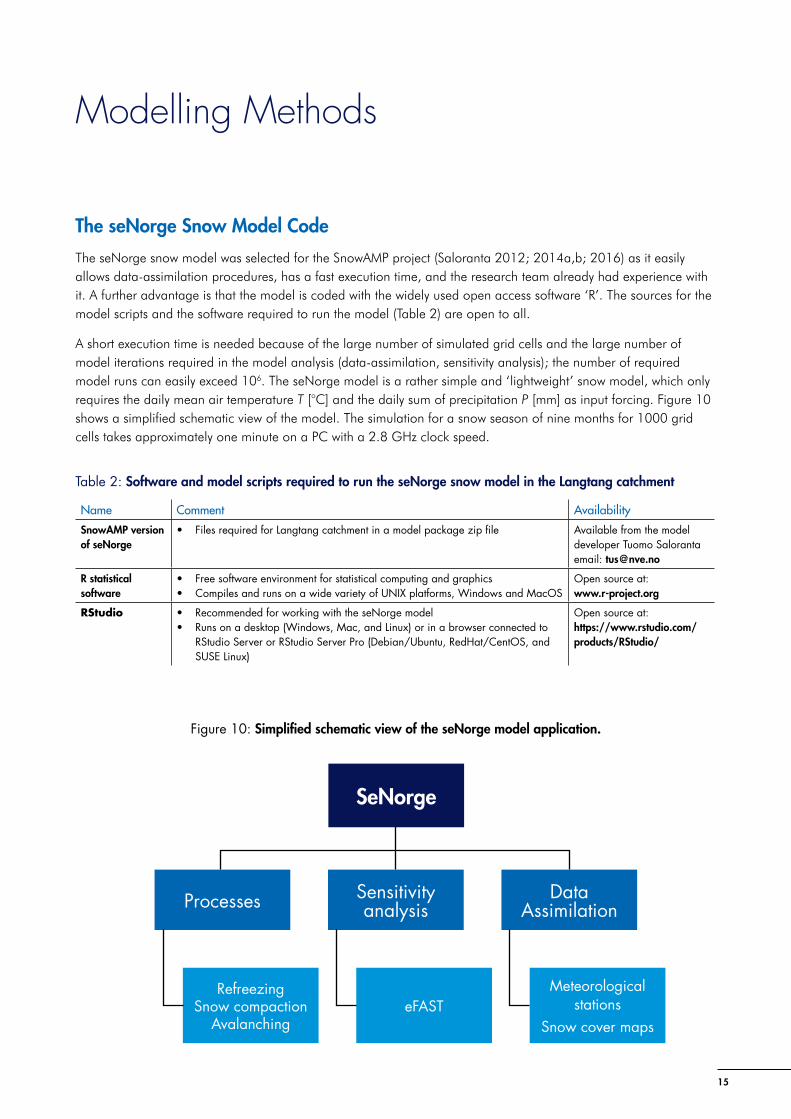
A short execution time is needed because of the large number of simulated grid cells and the large number of model iterations required in the model analysis (data-assimilation, sensitivity analysis); the number of required model runs can easily exceed 106. The seNorge model is a rather simple and ‘lightweight’ snow model, which only requires the daily mean air temperature T [°C] and the daily sum of precipitation P [mm] as input forcing. Figure 10 shows a simplified schematic view of the model. The simulation for a snow season of nine months for 1000 grid cells takes approximately one minute on a PC with a 2.8 GHz clock speed.

Table 2: Software and model scripts required to run the seNorge snow model in the Langtang catchment

Name Comment Availability

SnowAMP version of seNorge

• Files required for Langtang catchment in a model package zip file Available from the model developer Tuomo Saloranta email: [email protected]

R statistical software

• Free software environment for statistical computing and graphics• Compiles and runs on a wide variety of UNIX platforms, Windows and MacOS

Open source at:www.r-project.org

RStudio • Recommended for working with the seNorge model • Runs on a desktop (Windows, Mac, and Linux) or in a browser connected to

RStudio Server or RStudio Server Pro (Debian/Ubuntu, RedHat/CentOS, and SUSE Linux)

Open source at:https://www.rstudio.com/products/RStudio/

Figure 10: Simplified schematic view of the seNorge model application.

Sensitivity analysis

eFAST

Data Assimilation

Meteorological stations

Snow cover maps

Processes

RefreezingSnow compaction

Avalanching

SeNorge

16

The seNorge snow model was revised to better simulate the snow processes in the Himalayan region, the revised version is referred to as the SnowAMP model. The following modifications were made:

� Solar radiation is calculated for inclined surfaces, and the albedo of the snow surface is taken into account in the snowmelt rate algorithm.

� A lognormal distribution is used to model the subgrid distribution of snow.

� Refreezing of liquid water in the snow pack is calculated using an algorithm based on Stefan’s law.

� The parameter file is simplified as the bias correction of input temperature and precipitation is handled in the model application script before executing the mode.

� Some bug fixes were carried out (see the code header).

The nine main model parameters and their default values in the revised code are summarized in Table 3. Some of the parameter values depend on whether the grid cell is above or below the tree line. Vertical gradient parameters for air temperature (Tvg) and precipitation (Pvg) are also introduced in order to remove systematic errors in the model input forcing (Table 3). These can be extended to piecewise linear functions in order to reflect the structure of the vertical (or even horizontal) temperature and precipitation gradients in more detail (see, for example, Immerzeel et al. 2012, 2014; Saloranta 2014a).

The equations in the previous seNorge snow model versions (v. 1.1 and v.1.1.1) are presented in detail in Saloranta (2012, 2014a, b, 2016). The SnowAMP version of the model is reviewed briefly in the following sections.

Snowmelt

The SWE submodel uses a threshold air temperature TS to separate snow and rain precipitation, handles the ice and liquid water fractions of the total SWE separately, and keeps track of the accumulation and melting of snow. The snowpack can retain liquid water from snowmelt and rain up to a fraction rmax of its ice content, while the excess goes to runoff. The liquid water in the snow pack can also be refrozen to ice.

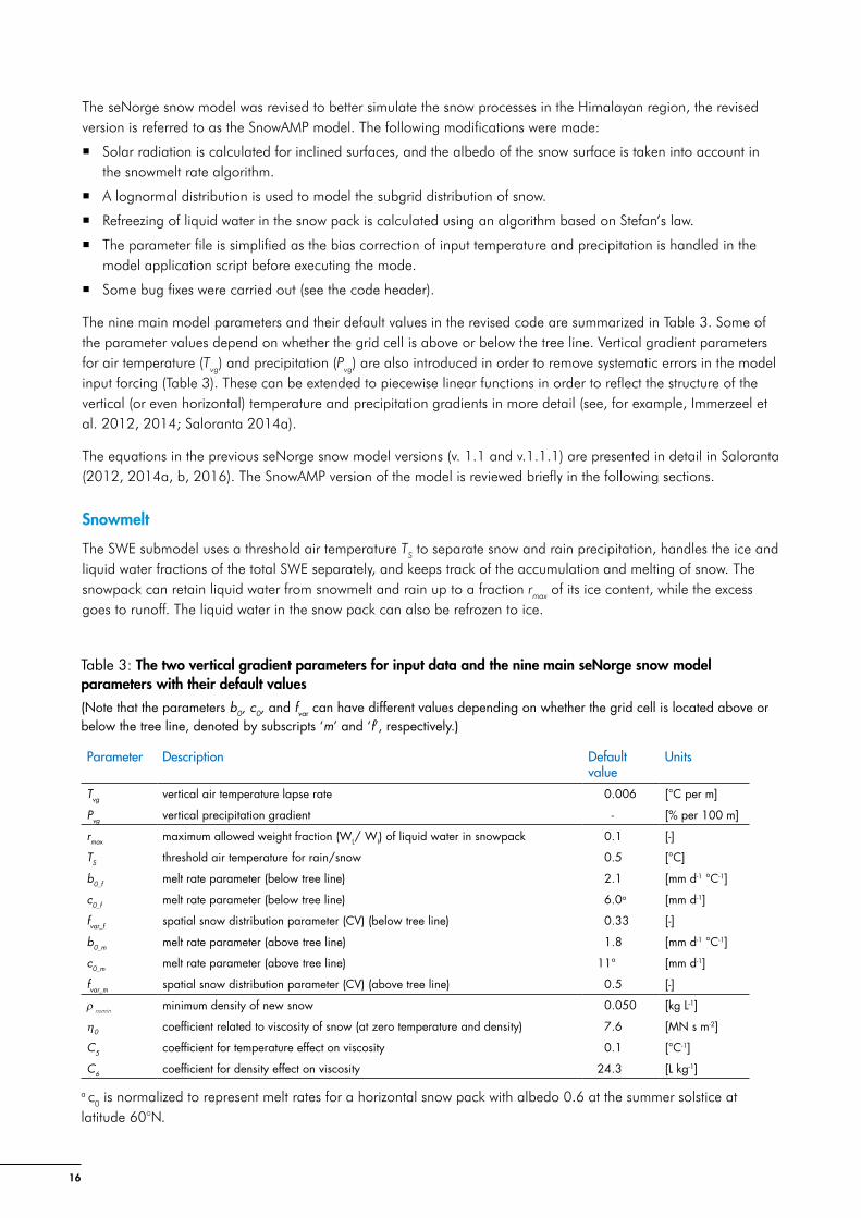
Table 3: The two vertical gradient parameters for input data and the nine main seNorge snow model parameters with their default values

(Note that the parameters b0, c0, and fvar can have different values depending on whether the grid cell is located above or below the tree line, denoted by subscripts ‘m’ and ‘f’, respectively.)

Parameter Description Default value

Units

Tvg vertical air temperature lapse rate 0.006 [°C per m]

Pvg vertical precipitation gradient - [% per 100 m]

rmax maximum allowed weight fraction (WL/ WI) of liquid water in snowpack 0.1 [-]

TS threshold air temperature for rain/snow 0.5 [°C]

b0_f melt rate parameter (below tree line) 2.1 [mm d-1 °C-1]

c0_f melt rate parameter (below tree line) 6.0a [mm d-1]

fvar_f spatial snow distribution parameter (CV) (below tree line) 0.33 [-]

b0_m melt rate parameter (above tree line) 1.8 [mm d-1 °C-1]

c0_m melt rate parameter (above tree line) 11a [mm d-1]

fvar_m spatial snow distribution parameter (CV) (above tree line) 0.5 [-]

ρ nsmin minimum density of new snow 0.050 [kg L-1]

h0 coefficient related to viscosity of snow (at zero temperature and density) 7.6 [MN s m-2]

C5 coefficient for temperature effect on viscosity 0.1 [°C-1]

C6 coefficient for density effect on viscosity 24.3 [L kg-1]

a c0 is normalized to represent melt rates for a horizontal snow pack with albedo 0.6 at the summer solstice at latitude 60°N.

17

The snowmelt simulation in the previous model code was based on a simple degree-day approach (e.g. Hock 2003), where the potential daily melting M* (actual melting M is limited by the availability of ice) was a product of the daily mean air temperature T and a degree-day factor CM [mm d-1 °C-1] varying with latitude and time of year.

This basic degree-day method, which is a common simplified way to represent snowmelt processes, is enhanced in the revised model with a solar radiation-related term to enforce its physical basis and improve model performance (Hock 2003). Snowmelt associated with this term is not dependent on air temperature but is related to the seasonal and zonal variation in incoming short-wave radiation. In the revised model code (v. 1.1.1), M* is formulated as

25

*00

* ScTbM , if T>0 °C (1) , if T>0 °C (1)

where b0 and c0 are empirical parameters and S* the daily solar irradiance [MJ d-1]. In the SnowAMP version of the model the formulation by Allen et al. (2006) is used, together with a snow albedo model (Tarboton and Luce 1996), where S* is the net shortwave radiation calculated for inclined grid cells with defined slope and aspect, taking into account the attenuation in the atmosphere as well as diffuse solar radiation (Hock 2003; Pellicciotti et al. 2005).

The values for parameters b0 and c0 (Table 1) are optimized using a statistical analysis of 3356 daily snowmelt rates from Norwegian snow pillow data (Saloranta 2014b). The value of c0 is furthermore normalized so that it has a physical meaning as a melt rate for a horizontal snow pack with albedo 0.6 at the summer solstice at latitude 60°N (the daily received solar radiation at the top of the atmosphere is approximately 40 MJ m-2 between latitudes 20–60°N at the summer solstice). Moreover, in the revised model, the grid cell average snowmelt rates are affected by the fraction of snow-covered area (SCA) in the grid cells considered (see below).

The seNorge snow model has been constructed to rely on only a few meteorological inputs, i.e. air temperature and precipitation, and avoid the use of more sophisticated, energy-balance snowmelt model algorithms (e.g. Armstrong and Brun 2008) which require additional inputs of shortwave and longwave radiation, wind, humidity, and air pressure. Comprehensive meteorological forcing data of this type are not often available with a suitable spatial resolution, quality, and robustness, thus simpler melt models are preferred (Hock 2003). Moreover, many studies, such as the snow model intercomparison project (Rutter et al. 2009), have shown that on average simpler snow models can perform as well as more complicated models.

Refreezing of liquid water in the snow pack

In the previous model (v.1.1.1), refreezing of liquid water within the snow pack was simulated in a rather simplified way, with the daily potential refreezing M*rf set equal to Crf.T, and Crf a constant model parameter (Table 3). This simple approach does not take into account the fact that liquid water in the top layer refreezes more easily than liquid water deeper in the snow pack, due to the thermal insulation effect of the snow. In the SnowAMP version of the model the refreezing algorithm is replaced by a more physically-based approach based on the modified Stefan’s law analytic model, originally developed for sea ice freezing (see, for example, Leppäranta 1993). In this approach, refreezing of liquid water is modelled in terms of a ‘refreezing front’ which proceeds from the top of the snow pack downwards. Whenever a new input of liquid water is added to the snow pack, either from snowmelt or rain, this refreezing front is brought back to the top of the snow pack, indicating that liquid water is present throughout the whole pack. In the SnowAMP model version, the depth of the refreezing front in the snow pack zrf [m] is formulated for a daily time step as:

28

tTL

zzlw

strf

trf

221 , if T 0 °C (2)

, if

28

tTL

zzlw

strf

trf

221 , if T 0 °C (2) (2)

Where Δt = 86,400 s, κs ([W m-1 K-1]) is the thermal conductivity of snow, L ([J kg-1]) is the latent heat of fusion, ρlw ([kg m-3]) is the partial density of the liquid water residing in the snow pack, and superscripts t and t-1 denote the present and previous time steps. Note that in the case of a snowfall PS ([mm]), the value of zrf t-1 must be adjusted by adding PS/ρs to it before using in Eq. 2. In addition, the upper limit for zrf is the snow depth.

18

The κs ([W m-1 K-1]) can be parameterized as a function of snow density (Yen 1981):

30

885.122362.2 ss (3) (3)

where ρs is the snow density (expressed in [kg L-1]).

A homogeneous distribution of liquid water in the snow pack below zrf is assumed, and the ρlw is simply the liquid water content WL [mm] divided by SD, which can be reformulated as ρlw = ρs.WL/SWE. Thus, for example, 40 mm of liquid water distributed evenly in a 1 m deep snow pack, gives ρlw= 40 kg m-3. As long as the SWE submodel is kept independent of the density submodel, a constant value for ρs is set, representative of the refreezing snow pack (e.g. 0.350 kg/L).

In the analytical Stefan’s law approach, an assumption is made of no thermal inertia (i.e. zero specific heat capacity) of the snow pack (Leppäranta 1993). This means that 1) refreezing due to the cold content of the snow pack is neglected and 2) the temperature profile in the snow pack is linear and adjusts instantly to the changing temperature at the top of the pack T0. Moreover, air temperature T is used to approximate T0, and the wet snow layer temperature below zrf is kept at the melting point (0°C).

The refreezing in the snow pack does not immediately change the SWE, since water is only transferred from the liquid to the solid phase. However, refreezing increases the ice fraction of the snow pack, which in turn increases the liquid water holding capacity of the pack in the model. Later, this again contributes to reducing runoff from the snow pack, as well as to increasing the snow density.

An additional advantage of the new algorithm is that the somewhat vaguely defined refreezing parameter Crf in model version (v.1.1.1) is no longer used. Now refreezing efficiency can be adjusted using the more physical and well-defined snow density parameter ρs, which affects refreezing efficiency both via κs and SD. This provides more effective heat conduction and a stronger temperature gradient.

In the model code, a lognormal-based snow distribution (see next section) and corresponding quantile bins are also used in the refreezing calculations. Daily refreezing Mrf [mm] can be estimated easily for each quantile bin from the liquid water content and the daily increase in zrf :

32

1,min trf

trflwLrf zzWM , if T 0 °C (4)

(4)

The total refreezing is then simply the sum of the refreezing in all the snow distribution quantile bins. This newly refrozen ice is simply subtracted from the snow pack liquid water fraction and added to the snow pack ice fraction.

Distribution of SWE and the fraction of snow-covered area in the model grid cells

Snow depth, and consequently SWE, shows a strong spatial variability (e.g. Clark et al. 2011). For example, in mountainous areas the interplay of topography and wind redistribution of snow can cause snow depths to vary from zero (bare ground) to a few meters over a short distance. In the previous seNorge snow model code (v.1.1.1), there was no simulation of spatial variability of SD or SWE within the model 1x1 km grid cells. In order to simulate 1) the subgrid spatial variability of SWE and 2) the fraction of snow-covered area (SCA) within the model grid cells, a new submodel is implemented in the revised model code (v.1.1.1). The main result is a reduction in the mean snow melting rate, and thus melt water discharge, for partly bare grid cells, i.e. when SCA<1. This effect is often especially pronounced in the late melting season. Furthermore, the simulated snow distribution and SCA allows for a quantitative model evaluation against observations of SCA and SD.

The new SCA submodel was inspired by the snow distribution algorithm in the VIC model (Cherkauer et al. 2003). The original model was based on a uniform snow distribution within the grid cells. In the SnowAMP version of the model, a lognormal distribution is applied within the model grid cells in order to allow a more skewed and realistic snow distributions (Marchand and Killingtveit 2005).

19

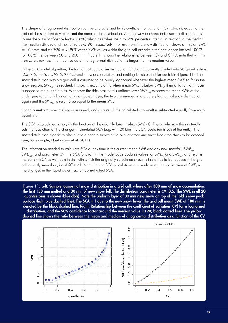
The shape of a lognormal distribution can be characterized by its coefficient of variation (CV) which is equal to the ratio of the standard deviation and the mean of the distribution. Another way to characterize such a distribution is to use the 90% confidence factor (CF90) which describes the 5 to 95% percentile interval in relation to the median (i.e. median divided and multiplied by CF90, respectively). For example, if a snow distribution shows a median SWE = 100 mm and a CF90 = 2, 90% of the SWE values within the grid cell are within the confidence interval 100/2 to 100*2, i.e. between 50 and 200 mm. Figure 11 shows the relationship between CV and CF90; note that with its non-zero skewness, the mean value of the lognormal distribution is larger than its median value.

In the SCA model algorithm, the lognormal cumulative distribution function is currently divided into 20 quantile-bins (2.5, 7.5, 12.5, …, 92.5, 97.5%) and snow accumulation and melting is calculated for each bin (Figure 11). The snow distribution within a grid cell is assumed to be purely lognormal whenever the highest mean SWE so far in the snow season, SWEHI, is reached. If snow is accumulating when mean SWE is below SWEHI, then a flat uniform layer is added to the quantile bins. Whenever the thickness of this uniform layer SWEbuff exceeds the mean SWE of the underlying (originally lognormally distributed) layer, the two are merged into a purely lognormal snow distribution again and the SWEHI is reset to be equal to the mean SWE.

Spatially uniform snow melting is assumed, and as a result the calculated snowmelt is subtracted equally from each quantile bin.

The SCA is calculated simply as the fraction of the quantile bins in which SWE>0. The bin-division then naturally sets the resolution of the changes in simulated SCA (e.g. with 20 bins the SCA resolution is 5% of the units). The snow distribution algorithm also allows a certain snowmelt to occur before any snow-free area starts to be exposed (see, for example, Duethmann et al. 2014).

The information needed to calculate SCA at any time is the current mean SWE and any new snowfall, SWEHI, SWEbuff, and parameter CV. The SCA function in the model code updates values for SWEHI and SWEbuff and returns the current SCA as well as a factor with which the originally calculated snowmelt rate has to be reduced if the grid cell is partly snow-free, i.e. if SCA <1. Note that the SCA calculations are made using the ice fraction of SWE, as the changes in the liquid water fraction do not affect SCA.

Figure 11: Left: Sample lognormal snow distribution in a grid cell, where after 300 mm of snow accumulation, the first 150 mm melted and 30 mm of new snow fell. The distribution parameter is CV=0.5. The SWE in all 20 quantile bins is shown (blue dots). Note the uniform layer of 30 mm new snow on top of the ‘old’ snow pack

surface (light blue dashed line). The SCA = 1 due to the new snow layer; the grid cell mean SWE of 180 mm is denoted by the black dashed line. Right: Relationship between the coefficient of variation (CV) for a lognormal

distribution, and the 90% confidence factor around the median value (CF90; black dotted line). The yellow dashed line shows the ratio between the mean and median of a lognormal distribution as a function of the CV.

CV versus CF90

90%

con

fiden

ce fa

ctor

(CF9

0)

CV

1.0

1

.5

2.0

2

.5

3.0

3

.5

4.0

0.0 0.2 0.4 0.6 0.8 1.0

SWE

quantile bin

0

100

300

500

0.0 0.2 0.4 0.6 0.8 1.0

20

Snow compaction and density submodel

The snow compaction and density submodel calculates changes in SD [mm] due to snowmelt and new snowfall events, as well as due to viscous compaction, where the compaction rate is dependent on the mass, density, temperature, and liquid water content of the snow pack. The density of newly fallen snow ρns [kg L-1] is a function of air temperature as in Bras (1990):

32

2

min 100)328.1(,0max

T

nsns (5) (5)

where ρnsmin is the minimum density of new snow (Table 3).

After taking into account the decrease of SD due to snowmelt and increase due to new snowfall (if any), the decrease of SD due to gradual compaction (ΔSDcomp) is calculated, making the assumption commonly used in snow models that snow behaves as a viscous medium (e.g. Yen 1981; Armstrong and Brun 2008):

36

tSDmSD Scomp

(6)

(6)

where ms is the force [Nm-2] due to the weight of the snowpack over the layer for which compaction is calculated, h is the viscosity of the snow [Ns m-2], and Δt is the time step(s). As we consider a single layer bulk snow pack, we set ms = 0.5gSWE, where g is the gravitation c onstant (9.81 m s-2). In the revised model (v.1.1.1), the equation for h follows the formulation in the Crocus snow model (Vionnet et al. 2012)

38

)exp(250.0601

1650 CTC

SDW snow

L

(7)

(7)

where WL ([mm]), Tsnow ([°C]), and ρ ([kg L-1]) are the liquid water content, temperature, and density of the snow pack, respectively. Tsnow is defined as the minimum between 0.5.Tair and 0. The constants h0, C5, and C6 are model parameters (see Table 3).

The SnowSlide algorithmThe SnowSlide algorithm (Bernhardt and Schultz 2010) is a fast and simple topographic (DEM) driven model for simulating the integral effects of gravitational snow transport due to avalanching activity. It can be used in connection with regularly gridded models and allows for snow transport between grid elements. SnowSlide is not a detailed avalanche model and thus cannot simulate the location of weak zones or the exact timing of snow slides and does not separate between starting, track, and run out zones. SnowSlide works in a continuous mode and can be executed in any time step of the hosting model if a defined snow holding depth (Shd) and a minimum slope angle (Sm) are exceeded. Based on manual calibrations, Bernhardt and Schultz (2010) set Sm to 25°. The value of Shd either depends on vegetation type or is based on a regression function (Bernhardt and Schultz 2010). The snow removed from a grid cell (i.e. the fraction of snow pack that exceeds the defined Shd) is redistributed to neighbouring grid cells located at lower elevation. This redistribution is proportional to the elevation difference between the snow source and the receiving neighbour grid cells (more snow is moved to grid cells with a larger elevation difference). The SnowSlide algorithm proceeds from the highest to the lowest grid cell in order to avoid snow transportation to already processed grid cells.

In the SnowAMP version of the seNorge model, the SnowSlide algorithm is placed in the model application file, since the main model code works only grid-cell-wise and cannot handle intergrid cell operations. The SnowSlide algorithm is set to redistribute snow between the grid cells at a given time step (e.g. every 10 days). The Sm is set to 25°, as in Bernhardt and Schultz (2010), and an exponential relation between slope angle Sa and Shd is applied, as proposed by Bernhardt and Schultz (2010):

40

)exp(1000 aEChd SppS (8)

(8)

21

where Shd [mm] is taken to represent the ice fraction of the total SWE in the grid cell, and parameter values pC and pE are set to 25 and -0.092. For example, slope angles of 35, 50, and 65° can hold 1000, 250 and 60 mm SWE of snow, respectively. As pointed out by Bernhardt and Schultz (2010) the parameters of Eq. 8 may be unique for each location and can be calibrated on the basis of remotely sensed or field campaign data.

Model sensitivity analysis (eFAST)

The purpose of model sensitivity analysis is to reveal the key parameters which affect the model output most and which should therefore be the ones that are later optimized to reduce the deviation between the model simulations and observations. Previous studies (e.g. He et al. 2011) have applied sensitivity analysis to a snow model for similar reasons. They point out that the influential parameters can vary from case to case depending on the output variables, year, season, and region, among others.

In the Langtang application, the sensitivity of the seNorge model was analysed using the extended Fourier Amplitude Sensitivity Test (eFAST) global sensitivity analysis method (Saltelli et al. 1999, 2000). In this method, the values for the model parameters are sampled in a wave-shaped form, so that the amplitude of the particular wave is equal to the parameter’s predefined feasible variation range. The frequencies of the waves are chosen to be orthogonal in such a way that none of the waves can be constructed as a linear combination of the other waves using integer coefficients up to a specific value. Each parameter is thus ‘labelled’ with its own frequency, and the sampling covers the whole multidimensional parameter space well. The model application is then run hundreds or thousands of times choosing a new set of parameter values from the wave-like parameter samples for each run, and the model output is monitored. Following this, the individual relative contributions of the different parameters to the model output variance can be identified from the periodogram based on the discrete Fourier transformation of the model output. The eFAST method reveals both the main effect of the parameter on the model output and the sum of the effects due to its higher-order interactions with other parameters. In interpreting the results, it is important to bear in mind that the sensitivity indices reflect both the role of the parameters in the model code and their predefined feasible value ranges (Figure 12). The definition of these ranges is normally based on data analysis, literature, and expert judgement.

Figure 12: Left: Example of the sensitivity indices from an eFAST sensitivity analysis where the output of interest was the mean snow water equivalent (SWE) in the Langtang catchment on 15 June 1982.

‘Main effect’ denotes the sensitivity index part explained by the particular parameter alone and ‘interaction’ the part explained by all parameter interactions where the particular parameter is included.

Right: The distribution of the mean snow water equivalent (SWE[mm]) in the Langtang catchment 15 June 1982 in 2200 model runs simulated with the different parameter sets in the eFAST analysis.

Freq

uenc

y

20 40 60 80 120 160

0

1

00

2

00

3

00

4

00

0.0 0.2 0.4 0.6 0.8 1.0

fvar_m

c0_m

b0_m

fvar_f

c0_f

b0_f

Crf

Ts

rmax

Pvg

Tvg

main effectsinteractions

22

Model application setup for Langtang (the seNorge model zip-package)

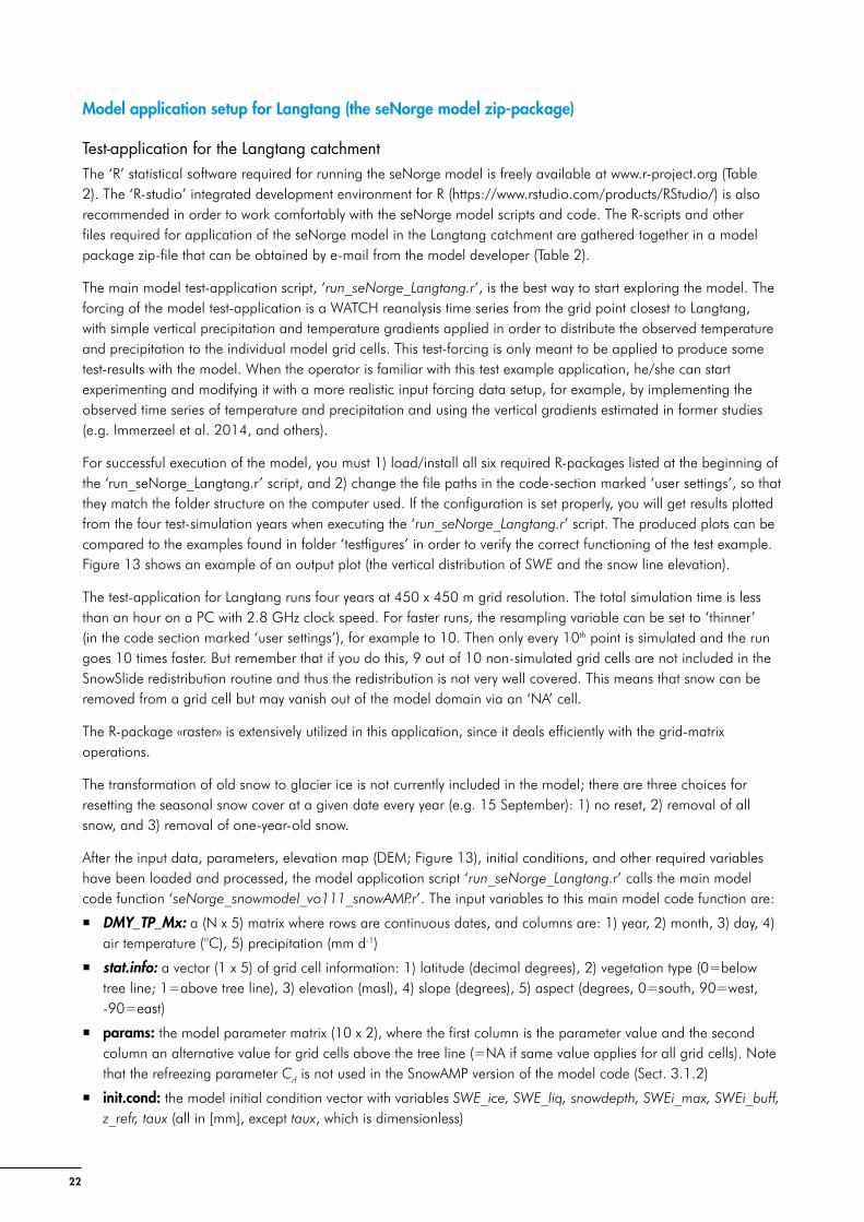
Test-application for the Langtang catchmentThe ‘R’ statistical software required for running the seNorge model is freely available at www.r-project.org (Table 2). The ‘R-studio’ integrated development environment for R (https://www.rstudio.com/products/RStudio/) is also recommended in order to work comfortably with the seNorge model scripts and code. The R-scripts and other files required for application of the seNorge model in the Langtang catchment are gathered together in a model package zip-file that can be obtained by e-mail from the model developer (Table 2).

The main model test-application script, ‘run_seNorge_Langtang.r’, is the best way to start exploring the model. The forcing of the model test-application is a WATCH reanalysis time series from the grid point closest to Langtang, with simple vertical precipitation and temperature gradients applied in order to distribute the observed temperature and precipitation to the individual model grid cells. This test-forcing is only meant to be applied to produce some test-results with the model. When the operator is familiar with this test example application, he/she can start experimenting and modifying it with a more realistic input forcing data setup, for example, by implementing the observed time series of temperature and precipitation and using the vertical gradients estimated in former studies (e.g. Immerzeel et al. 2014, and others).

For successful execution of the model, you must 1) load/install all six required R-packages listed at the beginning of the ‘run_seNorge_Langtang.r’ script, and 2) change the file paths in the code-section marked ‘user settings’, so that they match the folder structure on the computer used. If the configuration is set properly, you will get results plotted from the four test-simulation years when executing the ‘run_seNorge_Langtang.r’ script. The produced plots can be compared to the examples found in folder ‘testfigures’ in order to verify the correct functioning of the test example. Figure 13 shows an example of an output plot (the vertical distribution of SWE and the snow line elevation).

The test-application for Langtang runs four years at 450 x 450 m grid resolution. The total simulation time is less than an hour on a PC with 2.8 GHz clock speed. For faster runs, the resampling variable can be set to ‘thinner’ (in the code section marked ‘user settings’), for example to 10. Then only every 10th point is simulated and the run goes 10 times faster. But remember that if you do this, 9 out of 10 non-simulated grid cells are not included in the SnowSlide redistribution routine and thus the redistribution is not very well covered. This means that snow can be removed from a grid cell but may vanish out of the model domain via an ‘NA’ cell.

The R-package «raster» is extensively utilized in this application, since it deals efficiently with the grid-matrix operations.

The transformation of old snow to glacier ice is not currently included in the model; there are three choices for resetting the seasonal snow cover at a given date every year (e.g. 15 September): 1) no reset, 2) removal of all snow, and 3) removal of one-year-old snow.

After the input data, parameters, elevation map (DEM; Figure 13), initial conditions, and other required variables have been loaded and processed, the model application script ‘run_seNorge_Langtang.r’ calls the main model code function ‘seNorge_snowmodel_vo111_snowAMP.r’. The input variables to this main model code function are:

� DMY_TP_Mx: a (N x 5) matrix where rows are continuous dates, and columns are: 1) year, 2) month, 3) day, 4) air temperature (°C), 5) precipitation (mm d-1)

� stat.info: a vector (1 x 5) of grid cell information: 1) latitude (decimal degrees), 2) vegetation type (0=below tree line; 1=above tree line), 3) elevation (masl), 4) slope (degrees), 5) aspect (degrees, 0=south, 90=west, -90=east)

� params: the model parameter matrix (10 x 2), where the first column is the parameter value and the second column an alternative value for grid cells above the tree line (=NA if same value applies for all grid cells). Note that the refreezing parameter Crf is not used in the SnowAMP version of the model code (Sect. 3.1.2)

� init.cond: the model initial condition vector with variables SWE_ice, SWE_liq, snowdepth, SWEi_max, SWEi_buff, z_refr, taux (all in [mm], except taux, which is dimensionless)

23

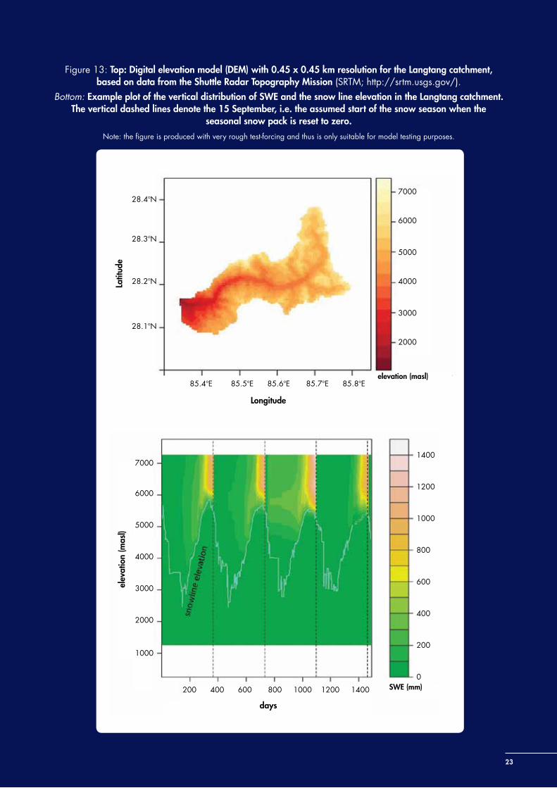
Figure 13: Top: Digital elevation model (DEM) with 0.45 x 0.45 km resolution for the Langtang catchment, based on data from the Shuttle Radar Topography Mission (SRTM; http://srtm.usgs.gov/).

Bottom: Example plot of the vertical distribution of SWE and the snow line elevation in the Langtang catchment. The vertical dashed lines denote the 15 September, i.e. the assumed start of the snow season when the

seasonal snow pack is reset to zero.

Note: the figure is produced with very rough test-forcing and thus is only suitable for model testing purposes.

28.4oN

28.3oN

28.2oN

28.1oN

7000

6000

5000

4000

3000

2000

Latit

ude

85.4oE 85.5oE 85.6oE 85.7oE 85.8oE

Longitude

elevation (masl)

days

1400

1200

1000

800

600

400

200

0

7000

6000

5000

4000

3000

2000

1000

200 400 600 800 1000 1200 1400

days

elev

atio

n (m

asl)

SWE (mm)

24

The output variables from this main model code function are:

� outDMY_TP_snow_Mx: a (N x 19) matrix where rows are continuous dates and columns are (see also definitions on last lines of the code): 1–5) DMY_TP_Mx as in input matrix, 6) snow water equivalent (SWE) (mm), 7) snow depth (mm), 8) snow density (kg L-1), 9) melting/refreezing rate (mm d-1), 10) runoff rate from snowpack (mm/d), 11) ratio of liquid water to ice (mm mm-1), 12) grid cell fraction of snow-covered area (SCA), 13-19) initial condition variables that can be used to define new initial conditions.

The main model code function ‘seNorge_snowmodel_vo111_snowAMP.r’ calls three different subfunctions: 1) ‘Albedo_UEB_TUS.r’ for calculation of the snow albedo, 2) ‘sca_logn_vo111_snowAMP.r’ for calculation of the subgrid snow distribution and snow-covered area, and 3) ‘solar_rad_Allen_TUS_mdf.r’ for calculation of the solar radiation flux.

Model sensitivity analysis test application for the Langtang catchmentThe seNorge model zip-package also includes an ‘R’ test-application script (‘run_sensitivity_Langtang.r’) to do the sensitivity analysis (see above) of the seNorge model application for the Langtang-catchment. The code in this eFAST sensitivity analysis script utilizes the ‘sensitivity’ R-package and has approximately the following code structure:

1. Settings for the model application defining the analysed output dates, as well as the min-max value ranges for the model parameters and other variables that are analysed in the sensitivity analysis; at present, the vertical gradients of temperature and precipitation (Tvg, Pvg) for distributing the test-forcing input to the different grid cells, as well as all the SWE-related model parameters, are included.

2. Loading the parameters, DEM, and forcing files of the Langtang model application

3. Letting the ‘fast99’ function construct the wave-like series for all the analysed parameters (placed in variable ‘phast’)

4. Start looping the model application repeatedly with all the different parameter sets produced by the ‘fast99’ function, writing selected output results on each simulation round to the variable ‘phast.res’, which is also saved after the looping. Any type of model output could be used, but here the mean snow water equivalent (SWE) and snow depth in the areas with snow (conditional SD), as well as the mean fraction of snow-covered area (SCA) and runoff, are selected.

5. Analysing (by Fourier transformation) the model outputs with the ‘fast99’ function, calculating the sensitivity indices, and plotting the results (see Figure 13). The vertical histogram-plots show the spread in the analysed model output values, corresponding to the different parameter value sets with which the model is run during the eFAST analysis. These plots can be used to check that the model results are within a plausible range. The horizontal histogram plots show the sensitivity indices for the analysed parameters. The higher the index, the more sensitive the output is for that parameter.

When you start working on this script you should, among others 1) modify the parameter selection in the sensitivity analysis to fit the input forcing setup and the uncertainties in it, 2) define the appropriate parameter ranges, and 3) select the most relevant model output for sensitivity analysis. In the test-application for sensitivity analysis, the whole catchment means are taken as output. In a refined sensitivity application, more specific model outputs could be defined, e.g. from different elevation intervals.

The total simulation time for the sensitivity analysis depends on the eFAST settings. For example, analysing the sensitivity of 11 parameters and setting variable ‘N.fast’ to 200, the total number of runs is 200*11 = 2200. If the variable ‘thinner’ is set to 25, i.e. simulating every 25th grid point (to give 124 grid points in the Langtang catchment), the total sensitivity analysis run takes about 15 hours on a PC with 2.8GHz clock speed.

25

Summary and Further Research

This document summarizes the achievements of the collaborative SnowAMP project up to spring 2016. The project aims to enhance the limited knowledge on snow cover dynamics, snowmelt, and the contribution of snowmelt to runoff in the Himalayas. The report describes the network of snow monitoring stations and installation during a field campaign in the Langtang valley in Nepal in autumn 2015, and presents the technical details of the seNorge snow model code (SnowAMP version, coded in ‘R’ statistical software) together with instructions on how to run it. An example application is available for the Langtang catchment.

Four snow monitoring stations have been installed along a south-north transect to enable monitoring of snow cover change with elevation. One extensively equipped station is installed at the foot of the south side of the Ganja La pass and three simpler stations on the north facing slopes of the pass inside the Langtang catchment. These instruments are complemented by a network of previously installed stations related to ICIMOD’s CMP project.

The seNorge model developed at NVE was chosen and a specific version adapted for snow modelling in the Langtang catchment. The model uses temperature and precipitation as inputs and provides snow-covered area, snow depth, and snow water equivalent as the main outputs. It takes into account the main snow pack processes such as snow accumulation, snowmelt (through an extended temperature index based parameterization), snow compaction, refreezing of meltwater in the snow pack, sub-grid distribution of snow water equivalent, and snow avalanching.

Modelling requires high quality input forcing data for the weather conditions and representative snow observations to evaluate the model results. One of the main aims of the SnowAMP project is to combine different snow data, such as ground-based and satellite-based data and the seNorge model outputs, using data-assimilation in order to provide useful, near real-time estimates of SWE in a remote Himalayan catchment. The activities in the final two years of the project will focus on

� maintaining the snow and weather monitoring stations,

� refining the seNorge snow model application for the Langtang catchment to provide more realistic snow simulations, and

� inclusion of ground-based and satellite-based snow data to evaluate model results and test the assimilation of these observations into the model.

Errors and uncertainties causing deviations between the simulated snow maps and snow observations may arise from

� the model structure, methods, and algorithms;

� the model parameter values;

� the input forcing data; and

� the observations.

Thus, the project will maintain a broad approach including both modelling and monitoring, in order to provide better and more accurate snow mapping in the catchment. The final aim is to provide more accurate estimates of the contribution of snow water melt to runoff over time, and the likely impacts of climate change on this value. The project is also a step forward towards providing real time estimates of snowmelt impacts on discharge.

26

References

Allen, RG; Trezza, R; Tasumi, M (2006) ‘Analytical integrated functions for daily solar radiation on slopes’. Agricultural and Forest Meteorology 139: 55-73

Armstrong, RL; Brun, E (2008) Snow and climate: Physical processes, surface energy exchange and modelling. Cambridge University Press, Cambridge, UK

Bernhardt, M; Schulz, K (2010) ‘SnowSlide: A simple routine for calculating gravitational snow transport’. Geophysical Research Letters 37 L 11502 DOI: 10.1029/2010GL043086

Bookhagen, B; Burbank, DW (2010) ‘Toward a complete Himalayan hydrological budget: Spatiotemporal distribution of snowmelt and rainfall and their impact on river discharge’. Journal of Geophysical Research 5 F03019 DOI: 10.1029/2009JF001426

Bras, RL (1990) Hydrology: An introduction to hydrologic science. Addison-Wesley, Reading, Mass. 643 pp.

Braun, LN, Grabs, W; Rana, B (1993) Application of a conceptual precipitation-runoff model in the Langtang Khola basin, Nepal Himalaya, Snow and Glacier Hydrology (Proceedings of the Kathmandu Symposium, November 1992). IAHS publication 218: 221-237

Cherkauer, KA, Bowling, LC; Lettenmaier, D (2003) ‘Variable infiltration capacity cold land process model updates.’ Global and Planetary Change 38: 151-159

Clark, MP; Hendrikx, J; Slater, AG; Kavetski, D; Anderson, B; Cullen, NJ; Kerr, T; Hreinsson, EÖ; Woods, A (2011) ‘Representing spatial variability of snow water equivalent in hydrologic and land-surface models: A review.’ Water Resources Research 47, W07539 DOI: 10.1029/2011WR010745

Collins DN; Davenport, JL; Stoffel, M (2013) ‘Climatic variation and runoff from partially-glacierised Himalayan tributary basins of the Ganges.’ Science of the Total Environment 468–469 (Suppl): S48–59

Duethmann, D; Peters, J; Blume, T; Vorogshyn, S; Güntner, A (2014) ‘The value of satellite-derived snow cover images for calibrating a hydrological model in snow-dominated catchments in Central Asia.’ Water Resources Research 50: 2002–2021 DOI: 10.1002/2013WR014382

He, M; Hogue, TS; Franz, KJ; Margulis, SA; Vrugt, JA (2011) ‘Characterizing parameter sensitivity and uncertainty for a snow model across hydroclimatic regimes.’ Advances in Water Resources 34: 114–127

Hock, R (2003) ‘Temperature index melt modelling in mountain areas.’ Journal of Hydrology 282: 104-115

Immerzeel, WW; van Beek, LPH; Bierkens, MFP (2010) ‘Climate change will affect the Asian water towers.’ Science 328(5984): 1382–1385

Immerzeel, WW; van Beek, LPH; Konz, M; Shrestha, AB; Bierkens, MFP (2012) ‘Hydrological response to climate change in a glacierized catchment in the Himalayas.’ Climatic Change 110: 721–736 DOI: 10.1007/s10584-011-0143-4

Immerzeel, WW; Pellicciotti, F; Bierkens, MFP (2013) ‘Rising river flows throughout the twenty-first century in two Himalayan glacierized watersheds.’ Nature Geoscience 6: 742-745 DOI: 10.1038/NGEO1896

Immerzeel, WW; Petersen, L; Ragettli, S; Pellicciotti, F (2014) ‘The importance of observed gradients of air temperature and precipitation for modelling runoff from a glacierized watershed in the Nepalese Himalayas.’ Water Resources Research 50: 2212-2226 DOI: 10.1002/2013WR014506

Kolberg, S; Gottschalk, L (2010) ‘Interannual stability of grid cell snow depletion curves as estimated from MODIS images.’ Water Resources Research 46, W11555 DOI: 10.1029/2008WR007617

Kolberg, S; Rue, H; Gottschalk, L (2006) A Bayesian spatial assimilation scheme for snow coverage observations in a gridded snow model.’ Hydrology and Earth System Sciences 10: 369-381

Lang, TJ; Barros, AP (2004) ‘Winter storms in the central Himalayas.’ Journal of the Meteorological Society of Japan 82(3): 829-844

27

Leppäranta, M (1993) ‘A review of analytical models of sea-ice growth.’ Atmosphere-Ocean 31: 123–138

Marchand, W-D; Killingtveit, Å (2005) ‘Statistical probability distributions of snow depth at the model sub-grid cell spatial scale.’ Hydrological Process 19: 355-369

Morinaga, Y; Seko, K; Takahashi, S (1987) ‘Seasonal variation of snowline in Langtang Valley, Nepal Himalayas, 1985-1986.’ Bulletin of Glacier Research 5: 49-53, Data Center for Glacier Research, Japanese Society of Snow and Ice

Parajka, J; Blöschl, G (2008) ‘The value of MODIS snow cover data in validating and calibrating conceptual hydrologic models.’ Journal of Hydrology 358: 240-258

Pellicciotti, F; Brock, B; Strasser, U; Burlando, P; Funk, M; Corripio, J (2005) ‘An enhanced temperature-index glacier melt model including the shortwave radiation balance: Development and testing for Haut Glacier d’Arolla, Switzerland.’ Journal of Glaciology 51: 573-587

Pellicciotti, F; Buergi, C; Immerzeel, WW; Konz, M; Shrestha, AB (2012) ‘Challenges and uncertainties in hydrological modelling of remote Hindu Kush–Karakoram–Himalayan (HKH) basins: Suggestions for calibration strategies.’ Mountain Research and Development 32: 39-50 DOI: 10.1659/MRD-JOURNAL-D-11-00092.1

Pradhananga NS; Kayastha, RB; Bhattarai, BC; Adhikari, TR; Pradhan, SC; Devkota, LP; Shrestha, AB; Mool PK (2014) ‘Estimation of discharge from Langtang River basin, Rasuwa Nepal, using a glacio-hydrological model.’ Annals of Glaciology 55: 223-230

Prasch M; Mauser, W; Weber M (2012) ‘Quantifying present and future glacier melt-water contribution to runoff in a central Himalayan river basin.’ The Cryosphere 7: 889-904 DOI: 10.5194/tc-7-889-2013

Rohrer, M; Salzmann, N; Stoffel, M; Kulkarni, AI (2013) ‘Missing (in-situ) snow cover data hampers climate change and runoff studies in the Greater Himalayas.’ Science of the Total Environment 468-469: S60-70 DOI: 10.1016/j.scitotenv.2013.09.056

Rutter, N; Essery, R; Pomeroy, J; Altimir, N; Andreadis, K; Baker, I; Barr, A; Bartlett, P; Boone, A; Deng, H; Douville, H; Dutra, E; Elder, K; Ellis, C; Feng, X; Gelfan, A; Goodbody, A; Gusev, Y; Gustafsson, D; HellströM, R; Hirabayashi, Y; Hirota, T; Jonas, T; Koren, V; Kuragina, A; Lettenmaier, D; Li, W-P; Luce, C; Martin, E; Nasonova, O; Pumpanen, J; Pyles, RD; Samuelsson, P; Sandells, M; SchäDler, G; Shmakin, A; Smirnova, TG; StäHli, M; StöCkli, R; Strasser, U; Su, H; Suzuki, K; Takata, K; Tanaka, K; Thompson, E; Vesala, T; Viterbo, P; Wiltshire, A; Xia, K; Xue, Y; Yamazaki, T (2009) ‘Evaluation of forest snow processes models (SnowMIP2).’ Journal of Geophysical Research 114, D06111 DOI: 10.1029/2008JD011063

Saloranta, TM (2012) ‘Simulating snow maps for Norway: Description and statistical evaluation of the seNorge snow model.’ The Cryosphere 6: 1323-1337

Saloranta, TM (2014a) ‘Simulating more accurate snow maps for Norway with MCMC parameter estimation method.’ The Cryosphere Discussions 8: 1973-2003 DOI: 10.5194/tcd-8-1973-2014

Saloranta, TM (2014b) New version (v.1.1.1) of the seNorge snow model and snow maps for Norway, Rapport 6-2014, Norwegian Water Resources and Energy Directorate, Oslo, Norway,30 pp., available at: http://webby.nve.no/publikasjoner/rapport/2014/rapport2014_06.pdf,

Saloranta, TM (2016) ‘Operational snow mapping with simplified data assimilation using the seNorge snow model.’ Journal of Hydrology 538: 314-325

Saltelli, A; Tarantola, S; Chan, KP-S; Scott, EM (1999) ‘A quantitative model-independent method for global sensitivity analysis of model output.’ Technometrics 41: 39-56

Saltelli, A; Chan, K; Scott, EM (2000) Sensitivity analysis, Wiley, New York, USA

Siderius, C; Biemans, H; Wiltshire, A; Rao, S; Franssen, WHP; Kumar P; Gosain, AK; van Vliet, MTH; Collins, DN (2013) ‘Snowmelt contributions to discharge of the Ganges.’ Science of the Total Environment 468–469(Suppl): S93–S101

Steinegger, U; Braun, LN; Kappenberger, G; Tartari, G (1993) Assessment of annual snow accumulation over the past 10 years at high elevations in the Langtang Region, Snow and Glacier Hydrology (Proceedings of the Kathmandu Symposium, November 1992), IAHS Publication 218, pp 155–166, International Association of Hydrological Sciences, Wallingford, UK

Tarboton, DG; Luce, CH (1996) Utah Energy Balance Snow Accumulation and Melt Model (UEB), Computer model technical description and users guide, Utah Water Research Laboratory and USDA Forest Service Intermountain Research Station, http://www.neng.usu.edu/cee/faculty/dtarb/snow/snowrep.pdf

28

Ueno, K; Shiraiwa, T; Yamada, T (1993) Precipitation environment in the Langtang Valley, Nepal Himalayas, Snow and Glacier Hydrology (Proceedings of the Kathmandu Symposium, November 1992), IAHS Publ. 218, pp. 207–219, International Association of Hydrological Sciences, Wallingford, UK

Vionnet, V; Brun, E; Morin, S; Boone, A; Faroux, S; Le Moigne, P; Martin, E; Willemet, J-M (2012) ‘The detailed snowpack scheme Crocus and its implementation in SURFEX v7.2.’ Geoscientific Model Development 5: 773-791

Yen, Y-C (1981) Review of thermal properties of snow, ice and sea ice. US Army Cold Regions Research and Engineering Laboratory (CRREL), Report 81-10, Hanover, NH, USA, 1981

29

30

© ICIMOD 2016International Centre for Integrated Mountain DevelopmentGPO Box 3226, Kathmandu, NepalTel +977 1 5003222 Fax +977 1 5003299Email [email protected] Web www.icimod.org

ISBN 978 92 9115 429 6