Measuring and Modeling Investment Behavior in a Social Network

University of Massachusetts BostonScholarWorks at UMass Boston

Graduate Masters Theses Doctoral Dissertations and Masters Theses

6-1-2012

Measuring and Modeling Investment Behavior in aSocial NetworkAlex DusenberyUniversity of Massachusetts Boston

Follow this and additional works at: http://scholarworks.umb.edu/masters_theses

Part of the Computer Sciences Commons, Economics Commons, and the Sociology Commons

This Open Access Thesis is brought to you for free and open access by the Doctoral Dissertations and Masters Theses at ScholarWorks at UMassBoston. It has been accepted for inclusion in Graduate Masters Theses by an authorized administrator of ScholarWorks at UMass Boston. For moreinformation, please contact [email protected].

Recommended CitationDusenbery, Alex, "Measuring and Modeling Investment Behavior in a Social Network" (2012). Graduate Masters Theses. Paper 92.

MEASURING AND MODELING INVESTMENT BEHAVIOR IN A SOCIAL

NETWORK

A Thesis Presented

by

ALEXANDER E. DUSENBERY

Submitted to the Office of Graduate Studies,University of Massachusetts Boston,

in partial fulfillment of the requirements for the degree of

Master of Science

June 2012

Computer Science Program

c© 2012 by Alexander E. DusenberyAll rights reserved

MEASURING AND MODELING INVESTMENT BEHAVIOR IN A SOCIAL

NETWORK

A Thesis Presented

by

ALEXANDER E. DUSENBERY

Approved as to style and content by:

Duc A. Tran, Assistant Professor,Chairperson of Committee

Timothy Killingback, Associate Professor,Member

Bala Sundaram, Professor,Member

Dan Simovici, Professor,Member

Dan Simovici, Program DirectorComputer Science Program

Peter Fejer, ChairpersonComputer Science Department

ABSTRACT

MEASURING AND MODELING INVESTMENT BEHAVIOR IN A SOCIAL

NETWORK

June 2012

Alexander E. Dusenbery

Directed by

Duc A. Tran, Assistant Professor

Over the past decade, a great deal of research has been done on the dynamics of complex

networks, particularly in the realm of social networks. As online social networks

(Facebook, LinkedIn, etc.) have exploded in popularity, a deluge of data has become

available to researchers, providing detailed histories of online social interaction. A

growing number of small-scale online networks aimed at certain niche groups of users

have also sprouted up, providing a richer context for the study of social network

dynamics. One such network is Currensee, which provides a social platform for investors

in the foreign exchange market. Through the dataset provided by Currensee, we are able

to study the investment activity of investors who participate in a social network focused on

their investment decisions. Furthermore, we can examine the aggregate investment

activity of this network in relation to general financial market volatility. After discovering

an interesting relationship between between market volatility and a certain measure of

iv

behavioral finance (“herding”), we lastly aim to simulate this type of investment network,

allowing us to control for network topology, and thus examine the impact of network

topology on the aggregate behavior of the investing agents composing said network.

v

TABLE OF CONTENTS

LIST OF FIGURES . . . . . . . . . . . . . . . . . . . . . . . . . . . . . . . vii

CHAPTER Page

1. NETWORK DESCRIPTION AND ANALYSIS . . . . . . . . . . 1

Introduction . . . . . . . . . . . . . . . . . . . . . . . . . . . 1

Background and Related Work . . . . . . . . . . . . . . . . . 2

The Currensee Dataset . . . . . . . . . . . . . . . . . . . . . 4

Analysis . . . . . . . . . . . . . . . . . . . . . . . . . . . . . 4

2. HERDING IN THE DATASET . . . . . . . . . . . . . . . . . . 12

Background . . . . . . . . . . . . . . . . . . . . . . . . . . . 12

Measurement of Herding . . . . . . . . . . . . . . . . . . . . 13

Empirical Herding Results . . . . . . . . . . . . . . . . . . . 16

3. HERDING IN A SIMPLE AGENT-BASED MODEL . . . . . . . 26

Model Motivation . . . . . . . . . . . . . . . . . . . . . . . . 27

Model Description . . . . . . . . . . . . . . . . . . . . . . . 28

Simulation Results . . . . . . . . . . . . . . . . . . . . . . . 33

Conclusion . . . . . . . . . . . . . . . . . . . . . . . . . . . 41

APPENDIX A: SIMULATION IMPLEMENTATION . . . . . . . . . 43

REFERENCE LIST . . . . . . . . . . . . . . . . . . . . . . . . . . . . . . . 45

vi

LIST OF FIGURES

Figure Page

1. Degree Distribution . . . . . . . . . . . . . . . . . . . . . . . . . 6

2. Mean Shortest Path Length . . . . . . . . . . . . . . . . . . . . . 6

3. Network Density and Degree Assortativity. . . . . . . . . . . . . . 7

4. Clustering and Transitivity . . . . . . . . . . . . . . . . . . . . . . 9

5. Distributions of User Activities. . . . . . . . . . . . . . . . . . . . 11

6. Daily Volatility . . . . . . . . . . . . . . . . . . . . . . . . . . . . 18

7. Daily Herding and VIX . . . . . . . . . . . . . . . . . . . . . . . 18

8. Daily Herding and VXY . . . . . . . . . . . . . . . . . . . . . . . 19

9. Daily Herding and CVIX . . . . . . . . . . . . . . . . . . . . . . 20

10. VIX and Volume . . . . . . . . . . . . . . . . . . . . . . . . . . . 22

11. CVIX and Volume . . . . . . . . . . . . . . . . . . . . . . . . . . 22

12. VXY and Volume . . . . . . . . . . . . . . . . . . . . . . . . . . 23

13. Herding and Volume . . . . . . . . . . . . . . . . . . . . . . . . . 24

14. Simulation results for s = 0 and n = 1000. . . . . . . . . . . . . . 34

15. Simulation results for s = 0.01 and n = 1000. . . . . . . . . . . . . 35

16. Simulations with s = 0.1 and n = 1000. . . . . . . . . . . . . . . . 38

17. Simulation experiment with s = 0.01 and pcopy = 0.1. . . . . . . . 40

18. Simulation experiment with s = 0.01 and pcopy = 0.1. . . . . . . . 41

vii

Figure Page

19. Implemenation of the Trading Network Simulation. . . . . . . . . 44

viii

CHAPTER 1

NETWORK DESCRIPTION AND ANALYSIS

1.1 Introduction

This thesis focuses on the analysis of a dataset describing the investment and online social

behavior of a set of individuals who are members of the online social network, Currensee.

It also presents an agent-based model of this network and its dynamics, through which we

explore how an interesting property of the network’s dynamics change with respect to

changes in the network’s structure. The approach is quite interdisciplinary in nature:

standard tools of social network analysis (SNA) are used to describe the topological

properties of the network from our dataset, while extensive examination of a particular

property from behavioral finance, “herding”, is made in the context of our dataset, as well

as in the simulation of our agent-based model. The aims of this thesis are the following:

1. To provide a unique case study of a type of social network not previously studied.

2. To apply a concept of behavioral finance to this dataset and measure the extent to

which this type of behavior occurs in the network.

3. To simulate a network with properties similar to the real network and observe the

changes in investment behavior with respect to changes in the network’s structure.

1

1.2 Background and Related Work

The foundation of complex network research is classically attributed to the work of Erdos

and Renyi and their random graph model [ER59]. In this model (ER), nodes in a network

are joined by an edge according to some fixed probability. Thus, the degree distribution of

a random graph approaches a Poisson distribution, in which most nodes have a degree that

is close to the average node degree. More recently, it has been observed that many real

networks diverge from the ER model. In some real-world networks, notably social

networks, node degrees tend to follow a Power-law distribution, where, for large degree k,

the fraction of nodes in the network having this degree is P(k) ∝ k−α , where α is the

power-law exponent of the degree distribution.

Over the last decade, researchers have become increasingly interested in the study of

online social networks (web-based platforms composed of users in often diverse physical

locations). Extremely popular websites like Facebook or LinkedIn are a very convenient

medium in which to keep in touch, find new friends, or search for employers. The

availability of data from such platforms has provided a means to examine some of the

sociological properties of these networks. This is important because the interactions of

individuals in a large social space can provide insight into the dynamics upon which

human social interaction is built.

The dataset focused on in this thesis is from Currensee, an online social network

aimed specifically at foreign currency exchange traders (Forex). The primary incentive for

an individual to join the Currensee network is to share their trading activity with others in

the network (this is, in a sense, similar to the idea of users sharing videos on YouTube). A

user may see, in real-time, the Forex trades (also referred to herein as “positions” or

2

“investments”) being placed by any of their friends in the network. Thus, our dataset

provides the unique opportunity to study social network dynamics and structure in the

context of the investment behavior of the network’s participants.

Adamic et al. presented one of the first empirical studies of online social networks (the

Club Nexus website of Stanford University) [ABA03]. A series of work analyzing popular

online social networks (Orkut, Flickr, YouTube, and Facebook) is presented

in [MGD06, VMCG09, MKG+08, MMG+07]. Each of these works found that the

respective networks exhibit small-world and scale-free properties, consistent with the

preferential attachment model [BA99]. We will similarly analyze the Currensee network

and determine if it, too exhibits the properties of a small-world network with a scale-free

degree distribution.

The evolution of user activities in online social networks has also been thoroughly

investigated. The activity networks of Facebook and Cyworld have been studied

in [VMCG09] and [CKE+08], and in [LH08] the authors studied user communication

patterns in an “Instant Messenger” network, using a dataset that contained over 300 billion

messages. Each of these studies concluded that homiphily is a driving force in user

interaction, with a strong tendancy for similar users (similar in location, sex, age, and the

like) to interact with one another. In the analysis presented in this chapter, the tendancy

for users with similar investment activity and success to interact with one and other will be

analyzed.

3

1.3 The Currensee Dataset

The social network of Currensee is composed of people who invest in Forex markets and

have linked their brokerage accounts (i.e. the outside accounts through which they

perform their Forex trades) to Currensee. Thus, the investment activity of a member of

this network is displayed on Currensee for others (often those with whom a user has

formed an online friendship link) to observe. This is the primary activity of the Currensee

social network, although many of the other traditional activities of online social network

are available to users: sending private messages, posting in public forums, sharing

pictures, and so on. A user may also utilize a public profile to display personal

information, publish the strategies she is using for a given position, and track the

performance of her or others’ trading performance over time.

Our dataset spans the range from the formation of the network in early 2009 through

November 30, 2010. We will consider the time at which a user completed his registration

to be the time at which he entered the network. The dataset does not reflect the time at

which friendship links were formed; therefore, we consider links to have formed between

two friends u and v at the time when user u sent a friendship request message to user v (or

visa versa).

1.4 Analysis

In this section, the general topological properties of the Currensee network are examined,

as well as the distribution of some user activities. All calculations of power-law exponents

use the fitting algorithm of Clauset et. al [CSN09]. As this particular network is still fairly

young and contains a relatively small number of users, we expect to see patterns of drastic

4

changes during the network’s early formation giving way to gradual changes or

stabilization as the network grows. Note that a portion of this dataset was analyzed

in [DNT12].

In what follows, we refer to the underlying graph of a social network as G(V,E),

where V is the set of vertices of G and E the set of edges connecting the vertices. We

consider G to be undirected. Furthermore, we define n = |V | and m = |E|.

1.4.1 Structural Properties of the Network

The social degree of a user is defined as the number of friendship links in which that user

takes part. While the network is relatively small, we expect to see a degree distribution

that approaches a power-law distribution. Figure 1 plots the social degree distribution as

well as the associated power-law exponent, α , for the minimum considered degree xmin

ranging from 0 to 100. Generally, a network’s degree distribution is said to follow a

power-law distribution if 2≤ α ≤ 3. We see that this property holds for the Currensee

network only when we take xmin ≥ 40 (roughly).

We define the diameter of a graph G as the average shortest path length from node u to

node v for all u,v ∈ G. Since the Currensee network is generally not connected (Figure

2b), we measure the diameter as the average shortest path length over nodes in the giant

component of the network. The giant component almost always accounts for 99 percent or

more of the network, so this gives a very close approximation. Figure 2a shows that the

diameter of the network increases steadily until about 15000 edges have formed in the

network, at which point it appears to converge to around 3.0, which is consistent with the

properties of a small-world network.

5

100 101 102 103 104

Degree

100

101

102

103

Count

(a) Degree distribution

0 20 40 60 80 100xmin

1.4

1.6

1.8

2.0

2.2

2.4

2.6

2.8

α

(b) Power-law exponent

Figure 1: Distribution of user social degree with corresonding plot of power-law exponents

varying by minimum degree considered.

(a) Network Diameter (b) Giant Component Size

Figure 2: Average shortest path length of the giant component of the Currensee network.

6

0 5000 10000 15000 20000 25000 30000 35000 40000Number of links

0.00

0.05

0.10

0.15

0.20

0.25

Netw

ork

Densi

ty

(a) Network Density

0 5000 10000 15000 20000 25000 30000 35000 40000Number of Edges

0.45

0.40

0.35

0.30

0.25

0.20

0.15

0.10

Degre

e A

ssort

ati

vit

y

(b) Degree Assortativity

Figure 3: Network Density and Degree Assortativity.

The density of an undirected graph G is defined as 2m/n(n−1); that is, the density of

a graph measures its completeness. A graph with 0 edges has density of 0 and a complete

graph has a density of 1. Figure 3a shows the density of the Currensee network as a

function of the number of edges in the network. It’s not surprising that the density

decreases very quickly and approaches a value less that 0.01.

An important metric of complex networks is the assortativity (or homiphily), which

measures the degree to which nodes in a network share edges with other nodes of similar

degree. One consequence of this preference is that highly connected nodes tend to form

links with other highly connected nodes. This preference for degree similarity exhibited

by a graph’s nodes is often refered to as assortative mixing, as it concerns the tendency for

individual nodes to pair with nodes of a similar ilk. Thus, we’ll call the actual

measurement of homophily in the network the network’s assortativity coefficient. As

Newman points out in [New03], for an undirected graph, assortativity can essentially be

measured using Pearson’s Correlation Coefficient. Figure 3b displays the assortativity

7

coefficient, which shows a sharp jump within the formation of the first 5000 edges.

Importantly, the Currensee network exhibits disassortative mixing, as indicated by a

negative assortativity coefficient. This negavite coefficient more closely resembles the

mixing patterns seen in technological (e.g. a client-server architecture) and biological

networks, rather than the positive coefficient generally seen in traditional social

networks [New02]. An important consequence of this disassortativity is that the network

(or it’s giant component) is less robust to the removal of vertices [New02]. So, while

networks that have power-law degree distributions are generally prone to “attack” via the

removal of highly connected nodes, matters are even worse in the case of this

disassortative network.

Many networks display a tendency for link formation between neighboring vertices,

which is usually refered to as clustering [WS98]. This tendency leads to dense local

neighborhoods, in which many neighbors of a single node tend to be connected

themselves. Two common measures of the degree of clustering within a network are

transitivity and the average clustering coefficient. Transitivity is defined as the ratio of all

possible triangles in a graph which are in fact triangles. A possible triangle, or “triad”, is a

set of two edges, (u,v) and (w,v) that share a vertex, v. If we also have (u,w) ∈ E, then

the three edges form an actual triangle. Thus, over a graph G, we can define transitivity as

3×|{triangles}|/|{triads}|. For a complete network, the transitivity is 1.0, and for an

empty network it’s 0.

We define the clustering coefficient of a vertex as

cv =2T (v)

d(v)(d(v)−1)

8

(a) Network Transitivity

0 5000 10000 15000 20000 25000 30000 35000 40000Number of links

0.2

0.3

0.4

0.5

0.6

0.7

Avera

ge C

lust

eri

ng C

oeff

icie

nt

(b) Average Clustering Coefficient

Figure 4: Average Clustering Coefficient and Network Transitivity

where T (v) is the number of triangles around v and d(v) is the degree of v. This is just the

fraction of possible triangles that actually exist around v. Thus, the average clustering

coefficient is

C(G) =1n ∑

v∈Gcv

and also attains values between 0 and 1.

Figure 4 gives the network transitivity and average clustering coefficient. Both exhibit

a similar pattern of decreasing quickly as the first 5000 edges form in the graph and then

appear to converge. The average clustering coefficient tells us (after a sufficient number of

link formations) that an average node has about 25 percent of possible triangles in its

neighborhood. Similarly, the transitivity plot shows that about 5 percent of all possible

triangles in the social graph actually exist. This suggests that the network is composed of

many local cliques which are likely connected by very high-degree hubs.

9

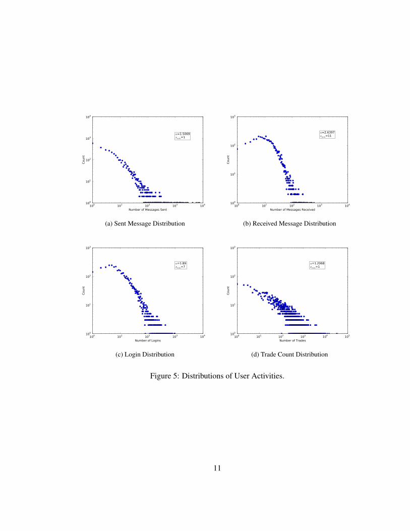
1.4.2 User Activity

We evaluate some of the user activity in terms of:

• The distribution of sent and received private messages.

• The distribution of site logins.

• The trade count distribution.

A user may send a private message to another user in the Currensee network whether a

friendship link exists between the two or not. Figures 5a and 5b show the distribution of

sent and recevied messages, respectively. Note that only the distribution of received

messages, with value α = 2.6397 for xmin = 11 is technically a power-law distribution

(that is, 2≤ α ≤ 3). The distribution of sent messages does not quite fit this requirement.

For comparison, note that a power-law distribution is also observed in the message activity

of Facebook [NT09].

Figure 5c shows the distribution of logins (that is, a pure count of the number of times

a user has logged-in to the Currensee web application) in the network. This distribution is

nearly power-law, with α = 1.89. We also have the distribution of user trades 1 in figure

5d. This distribution has the lowest “power-law exponent”, with α = 1.2068. Note that

the several users who have executed over 10,000 positions likely make use of some

automated-trading software for high-frequency trading.

1The term “trade” here is synonymous with “position”: an investor may initiate a long position on theEUR/USD at time t and close this position at some later time, t + k. Although two seperate orders have to beplaced in this scenario, it constitutes a single position. Note that, in more complex scenarios, such as a userclosing half of his initial order (akin to selling half of the shares he currently holds) at time t + j, the businesslogic of Currensee’s application records two different position “objects”, one long position that is marked asclosed at time = t + j of half the original buy order size, and another also of half the original size that remainsopen.

10

100 101 102 103 104

Number of Messages Sent

100

101

102

103

104

Count

α=1.5069xmin=1

(a) Sent Message Distribution

100 101 102 103 104

Number of Messages Received

100

101

102

103

Count

α=2.6397xmin=11

(b) Received Message Distribution

100 101 102 103 104

Number of Logins

100

101

102

103

Count

α=1.89xmin=7

(c) Login Distribution

100 101 102 103 104 105

Number of Trades

100

101

102

103

Count

α=1.2068xmin=1

(d) Trade Count Distribution

Figure 5: Distributions of User Activities.

11

CHAPTER 2

HERDING IN THE DATASET

2.1 Background

Our dataset contains information on the links established between users of a network, as

well as the trading history of each of the users in the network. Given this data, it is natural

to ask what effect these social ties between users have on the investment behavior

exhibited in the network. It has been suggested previously that institutional traders (i.e.

fund managers) exhibit a certain “copycat” tendency in their trading behavior, whereby

traders observe the trading behavior of other traders they know and use this information to

determine the buying or selling of stocks, rather than basing their investment decisions on

only their independent beliefs about a given instrument. This behavior is usually referred

to in behavioral finance literature as “herding” and is thought by some to result in unstable

stock prices, increased volatility, and the emergence of investment bubbles.

It is typically the case that institutional investors have access to the order history of

other institutions, so in that realm, it makes sense to consider herding behavior as a market

force, especially given the volume of orders placed by large financial institutions. One

may wonder to what degree individual traders display herding behavior, if at all. This is

generally hard to ascertain, since we usually cannot determine for some set of individuals,

12

whether those individuals have access to the investment decisions made by other

individuals in the same set.

In our dataset, we know the friendship ties that exist between all traders in the

network. Since this network allows a member to see the real-time trading history of any of

that member’s friends, we can assume that there is a level of shared information at least as

prevalent as that among institutional traders. Therefore, we can determine if herding

behavior occurs in a network of individual foreign exchange traders.

Individual foreign exchange traders, or even small foreign exchange trading

businesses, account for only a small fraction of the total volume exchanged daily in

foreign currencies, so we do not expect herding behavior to actually cause exchange price

destabilization or investment bubbles. Rather, we are more interested in observing how the

herding behavior among individual traders fluctuates in response to the state of the market

(or really, several markets) as a whole.

2.2 Measurement of Herding

Lakonishok et al. performed one of the first evaluations of herding behavior among

institutional investors [LSV92]. This study concluded that the level of herding among

institutional investors is relatively low, and that this behavior does not significantly effect

stock prices. It also provided a simple measure for assessing the level of herding among a

group of investors. They provide an illustrative example along these lines: suppose that, in

a given quarter, if we look across all stocks traded by all of the money managers among a

group of institutions, half of the changes in holdings (every trade is a change in holding)

of stocks are increases and the other half are decreases. Now, suppose that half of the

13

traders in this group had a net increase of holdings of most stocks in their portfolio, while

the other half of traders had a net decrease of holdings of most stocks in their portfolio.

That is to say, over some period, any one trade of a stock has an equal probability of being

a buy (increase in holding) or sell (decrease in holding), and that among all of the traders

in a group, half were net buyers and the other half were net sellers. In this scenario, we

would say that there is no herding (or at least no measurable herding) among this group of

traders and the set of assets which they invest in.

In another scenario, suppose still that any given trade in a period has an equal

probability of being a buy or a sell. Now, however, let us assume that 70% of traders in the

period were net buyers, and the other 30% were sellers of several assets. Also, for other

assets, assume that 70% of the traders had a net decrease in holdings and the other 30%

had a net incrase in holdings. This is a scenario in which herding occurs - the distribution

of buy transactions and sell transactions of a given asset is far removed from what we

would expect, given the equal probability of a single transaction to be a buy or sell.

While the above example is in terms of stocks traded by institutional investors, we can

just as easily apply it to individual foreign exchange investors. We consider currency

exchange pairs (for example, the Euro(EUR)/U.S. Dollar(USD) or U.S. Dollar/Japanese

Yen(JPY)) as the instruments being bought and sold, and consider an investor to be a net

buyer of a currency pair for a given period if the total volume of buy (sometimes referred

to as “long”) trades exceeds the total volume of sell trades (also known as “short” trades),

and similarly for net sellers. While the period over which herding is measured among

institutional stock traders is usually a quarter, the frequency of trades made by the foreign

exchange investors in our dataset is very high, so we typically consider a period of a single

trading day.

14

For a period t, we define Bt(i) as the number of net buyers of instrument i. Similarly,

St(i) is defined as the number of net sellers of instrument i in period t. If there are a total of

nit transactions involving instrument i in period t, then we define the buy ratio bri(t) as the

ratio of buy transactions of i relative to the total number of transactions of i over t. That is,

bri(t) =bi(t)nit

where bi(t) is the number of buy transactions of i occurring during t. Since the number of

net buyers Bt(i) follows a binomial distribution, bri(t) is a binomially distributed random

variable. Now, if we think about the probability of an individual investor buying a certain

instrument in some period, we can see that this probability pit is determined by the

probability of buying any instrument in time t in addition to the degree of herding for the

instrument i in time t. In other words, any individual buys an instrument during some

period according to whatever the overall probability is of that instrument being bought,

plus whatever effect the degree of herding has on buying that instrument in that period.

We define the probability of buying i during time t as

pit = brt +hit

where br(t) is the total buy ratio of all stocks at time t and hit is the degree of herding for

instrument i at t.

The total buy ratio br(t) for a period is just the average of the buy ratio for each

instrument in question over that period:

br(t) =∑i bri(t)

∑i nit.

The idea behind the measure of herding presented by Lakonishok et al. is to measure how

different the observed probability of buying an instrument i is from the overall probability

15

of buying any instrument during a period compared to the expected value of that

difference. Thus, the degree of herding for i at t is defined as:

hit = |bri(t)−br(t)|−E[|bri(t)−br(t)|].

This second term, the expected value of the difference between the buy ratio of i and the

total buy ratio, is included for the following reason: suppose that there is no herding effect

at all in a period. It is still extremely unlikely that the difference between the probability

of a trader buying a particular instrument and the probability of a trader making a buy

transaction of any instrument will be zero, particularly when the number of buy

transactions on instrument i is relatively small. Thus, we include this term to account for

the variance in the number of transactions. As the number of transactions grows larger,

this term will tend toward zero. Since bri(t) is a binomially distributed random variable,

and we have nit transaction observations over t, we can caluclate this expected difference

as [Kre10]:

E[|bri(t)−br(t)|] =nit

∑k=0

(nit

k

)br(t)k(1−br(t))nit−k

∣∣∣∣ knit−br(t)

∣∣∣∣.2.3 Empirical Herding Results

For this dataset, herding is measured daily from June 1, 2009 through November 29, 2010.

A subset of the 5 most commonly traded currency pairs is considered, which pairs are the

EUR/USD, USD/Canadian Dollar(CAD), Great Britain Pound(GBP)/USD, Australian

Dollar(AUD)/USD, and USD/JPY. For each trading day, we compute hit for each of these

instruments, and then a weighted daily average ht , where the weights correspond to nit/nt ,

the ratio of the number of transactions of instrument i on day t to the total number of

transactions on day t. Following other studies of institutional herding, hit is only

16

computed if bit ≥ 5. The weighted average of ht over all of the days in the data range

above, which will be denoted H, is 2.06%, with a standard error of the weighted mean of

.0017 (H is weighted by nt). Thus, for every 100 transactions made by individual traders

in our network, 2 more of those transactions landed on the same side of the market than

compared to a situation in which no herding occurred. While this might seem low, it is not

unexpected. As Lakonishok points out, in the foreign exchange market (or any market) as

a whole, there cannot be any herding, as for every share of an instrument bought, there is

one share that is sold.

In this section, we first study the way in which mean daily herding values relate to

volatility in financial markets. This should give some sense of how individual herding

behavior changes with respect to aggregate market conditions.

2.3.1 Herding in Relation to Market Volatility

We would like to see how the level of herding in the network changes with respect to

market volatility. We would like to know if herding increases in times of high volatility, if

it decreases during times of high volatility, or if there is no relationship between herding

and market volatility. We consider 3 volatility indices: the VIX [Wha09], which measures

implied volatility in the S&P 500; the CVIX, which is a cross-section version of the VIX;

and the VXY, which measures implied volatility in the currencies of the G7. Figure 6

shows each of these indices over a time period covering the span of our data set. In order

to examine the relationship between these volatility indices and the mean daily herding

values of the social network, the mean and median of the mean daily herding values on

days where the volatility indices fall within certain ranges has been plotted.

17

Jan 2009 Apr 2009 Jul 2009 Oct 2009 Jan 2010 Apr 2010 Jul 2010 Oct 2010Day

10

20

30

40

50

60

Implie

d V

ola

tilit

y

VIXVXYCVIX

Figure 6: Daily volatility indecies from January 1, 2009 through December 31, 2010.

15 20 25 30 35 40 45 50VIX Volatility Level (Day t)

0.000

0.005

0.010

0.015

0.020

0.025

0.030

0.035

0.040

Mean D

aily

Herd

ing (

Day t

)

Global MeanMeanMedian

(a) Mean and Median of Mean Daily Herding

15 20 25 30 35 40 45 50VIX Volatility Level

0

10

20

30

40

50

60

70

80

90

100

110

120

130

140

150

160

Num

ber

of

Days

MeanCount

(b) Number of Occurences of VIX Index Values

Figure 7: Plot of the Mean and Median of Mean Daily Herding values on days in which

the VIX index fell between different minimum and maximum values, with a distribution of

VIX index values within the same ranges.

18

10 11 12 13 14 15 16 17VXY Volatility Level (Day t)

0.000

0.005

0.010

0.015

0.020

0.025

0.030

Mean D

aily

Herd

ing (

Day t

)

Global MeanMeanMedian

(a) Mean and Median of Mean Daily Herding

10 11 12 13 14 15 16 17VXY Volatility Level

0

10

20

30

40

50

60

70

80

90

100

110

120

130

140

150

160

Num

ber

of

Days

MeanCount

(b) Number of Occurences of VXY Index Values

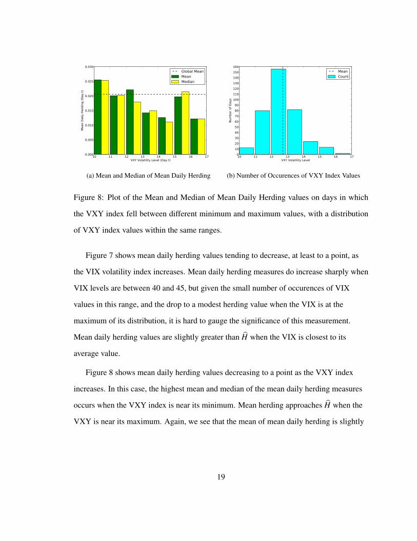
Figure 8: Plot of the Mean and Median of Mean Daily Herding values on days in which

the VXY index fell between different minimum and maximum values, with a distribution

of VXY index values within the same ranges.

Figure 7 shows mean daily herding values tending to decrease, at least to a point, as

the VIX volatility index increases. Mean daily herding measures do increase sharply when

VIX levels are between 40 and 45, but given the small number of occurences of VIX

values in this range, and the drop to a modest herding value when the VIX is at the

maximum of its distribution, it is hard to gauge the significance of this measurement.

Mean daily herding values are slightly greater than H when the VIX is closest to its

average value.

Figure 8 shows mean daily herding values decreasing to a point as the VXY index

increases. In this case, the highest mean and median of the mean daily herding measures

occurs when the VXY index is near its minimum. Mean herding approaches H when the

VXY is near its maximum. Again, we see that the mean of mean daily herding is slightly

19

10 11 12 13 14 15 16 17CVIX Volatility Level (Day t)

0.000

0.005

0.010

0.015

0.020

0.025

0.030

0.035

0.040

Mean D

aily

Herd

ing (

Day t

)

Global MeanMeanMedian

(a) Mean and Median of Mean Daily Herding

10 11 12 13 14 15 16 17CVIX Volatility Level

0

10

20

30

40

50

60

70

80

90

100

110

120

130

140

150

160

Num

ber

of

Days

MeanCount

(b) Number of Occurences of CVIX Index Values

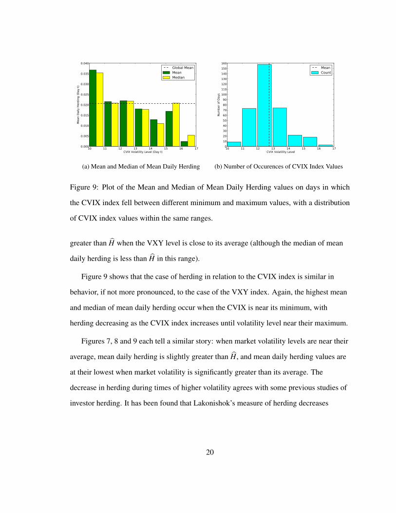
Figure 9: Plot of the Mean and Median of Mean Daily Herding values on days in which

the CVIX index fell between different minimum and maximum values, with a distribution

of CVIX index values within the same ranges.

greater than H when the VXY level is close to its average (although the median of mean

daily herding is less than H in this range).

Figure 9 shows that the case of herding in relation to the CVIX index is similar in

behavior, if not more pronounced, to the case of the VXY index. Again, the highest mean

and median of mean daily herding occur when the CVIX is near its minimum, with

herding decreasing as the CVIX index increases until volatility level near their maximum.

Figures 7, 8 and 9 each tell a similar story: when market volatility levels are near their

average, mean daily herding is slightly greater than H, and mean daily herding values are

at their lowest when market volatility is significantly greater than its average. The

decrease in herding during times of higher volatility agrees with some previous studies of

investor herding. It has been found that Lakonishok’s measure of herding decreases

20

among investments in volatile Portugese mutual funds [LS07]. The authors of this study

suggest that this may occur because higher volatility results in new information being

available to investors, so that investors rely less heavily on their knowledge of how other

investors are behaving. If this is the case, then herding should occur to a lesser degree. As

a counter-point, the authors of [HS01], , using their own measure of herding, find that

herding “toward the market portfolio” occurs more strongly in the US, UK and South

Korean stock markets when there is greater volatility in those markets.

2.3.2 Trading Volume and Market Volatility

To get a more precise notion of the significance of our herding results, we need to examine

the aggregate level of trading activity in relation to our measures of volatility. This can be

accomplished most simply by measuring the daily volume of trades in our network and

comparing it to daily volatility. We define the daily volume to be the sum of the volumes

of all positions opened on a given day 1.

Examining the relationship between trading volume and volatility does not tell us

much about our herding results on its own: we will see that, for our relatively small set of

individual investors, daily volume will decrease on days in which volatility is high.

However, looking ahead, we will be able to combine what we know about this relationship

with the relationship between herding and volume to extract more meaning from our

results on herding in relation to volatility.

As figures 10b, 11b and 12b show, the trading volume in our dataset generally

decreases on days in which volatility is high. This suggests that investors in the network

1It may seem more intuitive to define the daily volume in terms of the sum of the volumes of the ordersthat are filled on a particular day. However, since our herding measurement is defined in terms of positions(that is, net sum and direction), representing volume in terms of position size is more representative.

21

10 20 30 40 50 60VIX Volatility

0.5

0.0

0.5

1.0

1.5

2.0

2.5

3.0

3.5

Daily

Volu

me

1e8

(a) VIX Index vs. Daily Volume

15 20 25 30 35 40 45 50 55 60VIX Volatility Value

0.0

0.2

0.4

0.6

0.8

1.0

Mean D

aily

Volu

me

1e8

(b) VIX Index vs Mean Daily Volume

Figure 10: Daily volume in relation to the VIX volatility index. There is a negative corre-

lation (-0.2654) between daily volume and the VIX volatility index in our dataset, which is

apparent from examining the mean daily volume in relation to values of the VIX.

10 12 14 16 18 20 22 24CVIX Volatility

0.5

0.0

0.5

1.0

1.5

2.0

2.5

3.0

3.5

Daily

Volu

me

1e8

(a) CVIX Index vs. Daily Volume

10 12 14 16 18 20 22CVIX Volatility Value

0.0

0.2

0.4

0.6

0.8

1.0

1.2

Mean D

aily

Volu

me

1e8

(b) CVIX Index vs. Mean Daily Volume

Figure 11: A modest negative correlation (-0.3140) exists between daily volume and the

CVIX index. This is clear from (b), in which we observe that mean daily volume decreases

with increasing values of the CVIX index.

22

10 12 14 16 18 20 22VXY Volatility

0.5

0.0

0.5

1.0

1.5

2.0

2.5

3.0

3.5

Daily

Volu

me

1e8

(a) VXY Index vs. Daily Volume

10 12 14 16 18 20 22VXY Volatility Value

0.0

0.2

0.4

0.6

0.8

1.0

1.2

Mean D

aily

Volu

me

1e8

(b) VXY Index vs. Mean Daily Volume

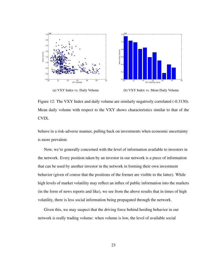
Figure 12: The VXY Index and daily volume are similarly negatively correlated (-0.3130).

Mean daily volume with respect to the VXY shows characteristics similar to that of the

CVIX.

behave in a risk-adverse manner, pulling back on investments when economic uncertainty

is more prevalent.

Now, we’re generally concerned with the level of information available to investors in

the network. Every position taken by an investor in our network is a piece of information

that can be used by another investor in the network in forming their own investment

behavior (given of course that the positions of the former are visible to the latter). While

high levels of market volatility may reflect an influx of public information into the markets

(in the form of news reports and like), we see from the above results that in times of high

volatility, there is less social information being propagated through the network.

Given this, we may suspect that the driving force behind herding behavior in our

network is really trading volume: when volume is low, the level of available social

23

0.5 0.0 0.5 1.0 1.5 2.0 2.5 3.0 3.5Daily Volume 1e8

0.06

0.04

0.02

0.00

0.02

0.04

0.06

0.08

0.10

Mean D

aily

Herd

ing

(a) Daily Volume vs. Mean Daily Herding

0.0 0.5 1.0 1.5 2.0 2.5 3.0 3.5Daily Volume Range 1e8

0.000

0.005

0.010

0.015

0.020

0.025

0.030

0.035

Mean D

aily

Herd

ing

(b) Daily Volume vs. Average Mean Daily Herding

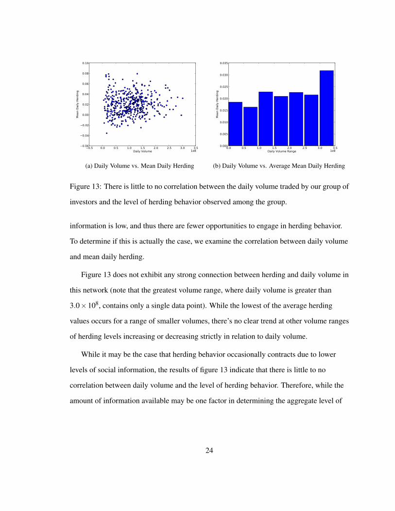
Figure 13: There is little to no correlation between the daily volume traded by our group of

investors and the level of herding behavior observed among the group.

information is low, and thus there are fewer opportunities to engage in herding behavior.

To determine if this is actually the case, we examine the correlation between daily volume

and mean daily herding.

Figure 13 does not exhibit any strong connection between herding and daily volume in

this network (note that the greatest volume range, where daily volume is greater than

3.0×108, contains only a single data point). While the lowest of the average herding

values occurs for a range of smaller volumes, there’s no clear trend at other volume ranges

of herding levels increasing or decreasing strictly in relation to daily volume.

While it may be the case that herding behavior occasionally contracts due to lower

levels of social information, the results of figure 13 indicate that there is little to no

correlation between daily volume and the level of herding behavior. Therefore, while the

amount of information available may be one factor in determining the aggregate level of

24

herding behavior, it appears that market volatility alone is a stronger herding predictor at

the level of individual investment. Thus, in periods of high market volatility, even if

investment activity among a group of investors is pronounced, we may fairly expect that

the degree to which the group herds toward the market portfolio is less than in a period of

lower volatility.

25

CHAPTER 3

HERDING IN A SIMPLE AGENT-BASED MODEL

It’s difficult to ascertain the relationship between the degree of herding and different

network statistics in the Currensee dataset. Examining subgraphs of the network which

are segregated by the statistical properties of the individual nodes in the subgraph is not

very fruitful. Furthermore, this does not yield any insight into how different network

structures effect the degree of herding behavior. Since there is no real, readily-available

data containing individual trading history in social networks of fundamentally different

structures, I’ll instead attempt to investigate the above-mentioned relationships through

the use of a simulated network model.

The field of agent-based computational finance has expanded in the last several

decades as research in finance has become more scientifically rigorous. This field utilizes

computational power to model artificial financial markets in cases where an analytical

solution would not be possible. The main draw of these computational models is that they

can simulate a market where the agents acting in the market differ in many ways.

Different agents may possess different levels of information, process information to

varying degrees, react to risk and volatility in different styles, and so on [LeB06].

26

3.1 Model Motivation

The agent-based model that we will use seeks to answer the question of how the degree of

herding in a network of connected agents is affected by the topology of the network. I am

not at all trained in economics or finance, and as such, I have aimed to develop as simple a

model as possible. Furthermore, so that the model might maintain at least a bit of

credibility in the realm of finance and economics, I have based the basic trading behavior

of agents in the model on the work of Cont [Con07] and Ghoulmie et al. [GCN05]. There

are several reasons for choosing this particular model. First, it is straight-forward and easy

to understand. As the authors claim, its simplicity lends to greater explanatory power.

Second, this model is capable of producing aggregate statistical properties similar to the

statistical properties of time series of real financial data.

In the empirical finance literature, a set of such properties which are common across

many markets, instruments, and time periods is often referred to as a “stylized fact”. One

of the more interesting stylized facts is that of volatility clustering: large changes of asset

returns (in either direction) tend to cluster together [Man63]. Furthermore, while it is

known that auto-correlations of asset returns are usually not significant, it is the case that

the absolute (or square) returns of assets do show a significant, slowly-decaying positive

autocorrelation over time ranging from minutes to weeks [Con01]. Lastly, it is noted that

trading volume is positively correlated with market volatility, and similar to the slow

decay of autocorrelation in volatility, trading volatility exhibits the same type of “long

memory” [LV00]. Cont’s model primarily aims to generate realistic volatility clustering

properties and suggests a link between volatility clustering and “investor inertia”. In

addition to utilizing a simple but believable financial model, it would also be desirable to

27

include a very simple mechanism for inducing herding behavior at an individual level.

The concept of herding is interesting in the context of complex networks because it

measures, in a broad sense, the aggregate degree to which individuals connected via a

social network are imitating the behavior of others in the network. Therefore, the herding

mechanism used in our simulation will simply be a propensity for traders to adopt the

trading strategy of one of their neighbors in a given trading period. The specifics of the

model are explained below.

3.2 Model Description

We want to model the following scenario: There is an empty network at the start of a

simulation. At a random interval, an agent joins the network and forms social links with

other agents in the network. In each simulation, we will specify beforehand the process by

which links form in the network. One set of simulations will have edges form according to

a random graph process in the style of Erdos and Renyi, by which each agent joining the

network has an equal probability plink of forming an edge connecting itself with another

agent already in the network.

Another set of simulations generates edges in the network according the “preferential

attachment” model of Barabasi and Albert, in which each agent is added to the network

with a constant number of edges that are preferentially attached to existing agents with

high degree [BA99]. A third set of similar situations generates network connections in a

similar way, although the resulting network has a higher clustering coefficient [HK02].

The last set of simulations will be performed on a complete graph, corresponding to a

well-mixed agent population in which any agent may interact with any other agent.

28

Comparing the case of a complete network to others in which a more refined attachment

mechanism is at play can indicate whether network structure really has any effect at all on

the degree of herding.

Each time-step of the simulation represents a single day. Every agent in the network

executes their trading strategy once a day. The agents execute their strategies in a different

random order each day. Agents have a choice of instruments that mirrors the five currency

exchange pairs used in the above empirical analysis of herding in a real financial network.

An agent can buy, sell, or do nothing with each instrument as part of their strategy. They

also, with a common probability, choose whether or not to copy the strategy of one of their

neighbors as part of executing their strategy on a given day.

The simulation program is written in the Python programming language using the

SimPy package. SimPy is an object-oriented, process-based discrete-event simulation

framework [MV03]. I chose to use this simulation package for its ease-of-use and because

of its implementation in a high-level, object-oriented language.

There are three basic components of the SimPy package: Processes, Resources and

Simulations (we don’t need Resources for our model implementation). Process objects are

the active objects in a simulation. Each Process object contains at least one “Process

Execution Method” that defines the behavior of that process. Our model implements

Agents, Agent Sources, and Trading Strategies as Process objects. Simulation objects run

the simulation of a model. In our model, a network of connected Agents that execute a

trading strategy is implemented as a Simulation object. The graph underlying the network

is implemented as a NetworkX Graph object [HSS08]. For any instrument i that can be

traded by the N agents in our model, we will denote the price of that instrument at time t

29

as Si,t . We use price data over an ordered sequence of real exchange rates in our model,

ranging from January 1, 2009 to November 20, 2010. 1

Trading takes place at discrete periods t = 0,1,2, ...,500. The agents in the model

form their trading behavior around the public information available and on their individual

decision thresholds. A real-world example of public information in the context of the

foreign exchange market is the monthly “Nonfarm Payrolls” employment report released

monthly by the United States Department of Labor. All investors in this or any other

market have the same access to this information, which would be relevant to any exchange

rate involving the U.S. Dollar.

For a basic idea of how agents behave in this model, think of a simple transition

function with three states: buy, sell, and do-nothing. Along the independent axis lie values

corresponding to the public signal, and along the dependent axis lie the three states.

Somewhere along the public signal axis lie two thresholds, and agent decisions are made

around these thresholds. When the public signal reaches a point below the lower

threshold, the function transitions into the sell state; when the public signal exceeds the

higher threshold, the function transitions to the buy state. At all points in between the two

thresholds, the function settles in the do-nothing state.

We model public information for an instrument i in our simulation as a sequence of

normally distributed random variables (εi,t |t = 0,1,2, ...,500) with εi,t ∼ N(µi,D2i ), where

µi is the average price of instrument i and Di is the standard deviation of i’s price. The

1The prices are the bid price at market open of each day. Note that we are not fully modeling a market. Inmany agent-based market simulations, the price of a particular asset is actually determined by the behaviorof the agents - whatever excess demand is generated for an asset by trading activity determines the price ofthe asset. Of course, this is the case in any real-world market, foreign currency exchange included. However,we’re dealing with a small enough subset of traders and volume (in both our real-world dataset and thus inour simulation) that we can basically ignore the effects of excess demand from the agents in our model.

30

idea behind this choice of εi,t is as follows: the public information ε is meant to represent

the input noise of our system. We want the amplitude of this noise to be chosen such as to

reproduce a realistic range of values for the annualized volatility of our instruments. 2

The decision threshold of each agent j,1≤ j ≤ N at time t with respect to instrument i

is denoted as the pair (θsell(i, j, t),θbuy(i, j, t)), where θsell(i, j, t)≤ θbuy(i, j, t). Cont

suggests that this threshold “be viewed as the agents (subjective) view on volatility.” The

threshold behavior is simple: if εi,t ≥ θbuy(i, j, t), then the agent places a buy order for

instrument i, if εi,t ≤ θsell(i, j, t), the agent places a sell order for instrument i. Otherwise,

the agent does not place an order for instrument i at time t. The initial values θ(i, j,0) are

drawn from a normal distribution N(µi,Di). We use the standard deviation and not the

variance in this case to get a more diverse range of agent behavior in the absence of an

update rule.

Real asset traders do not all have the same tolerance for volatility, nor does an

individual trader maintain a constant tolerance for volatility over time. Thus, the model

we use includes an update rule for agent thresholds. The rule is very simple: at each time

step, an agent j has some probability 0≤ s≤ 1 of updating her theshold θ(i, j, t). When

an agent updates his theshold, he increments it by the most recent return on instrument i,

which is ln Si,tSi,t−1

. 3 Cont suggests a value of s in the range 10−1−10−3. We will perform

simulations at various values of s, including s = 0, to examine what effect this parameter

has on the the herding results for the system.

2Note that these are on the order of 10−3.3Any time calculations revolving around probabilities occur in the Process Execution Method of a Process

object (Agents, Strategies, Sources), we make use of the SciPy stats package to draw a uniform randomvariable and compare it to the probability in question [JOP+ ].

31

3.2.1 Social Interaction in the Model

The model as originally presented by Cont does not include any mechanism for

interaction between agents. This makes sense from his perspective, of course, as his aim

was to produce realistic price data having properties similar to the stylized facts of

volatility in financial markets. However, our goal is different: rather than examining the

aggregate properties of prices and returns in an agent-based market, we assume a scenario

where price information is given as input to a small subset of individuals in a market and

examine the aggregate behavior of the individuals.

While we have found a simple model that is good at producing realistic properties of

prices over a time series in a market, we need to add a simple mechanism by which agents

in our model interact with each other if we want to examine the properties of social

behavior in a market over time. Because the particular behavior we are interested in is the

imitation of strategies, we will include a simple “copy” rule: at each time step t, for each

instrument i, an agent j has probability pcopy of substituting one of her neighbors k

thresholds θ(i,k, t) for her own. At time t +1, j resets her threshold to θ(i, j, t). This rule

allows us to represent a very simple type of imitation behavior, where an agent copies the

behavior of one of her neighbors for a given turn with some frequency. Of course, this is

not a very rational implementation of agent behavior. A rational agent would not copy one

of her neighbors randomly, but more likely give preference to copying the behavior of an

agent that has exhibited superior performance. There are two reasons for implementing an

irrational, random imitation rule in this framework:

• There is no notion of agent “performance” in this simulation, simply because we

have no need to track performance for the calculation of herding.

32

• Adding an imitation preference would only further complicate the model and lend

to more difficulty in interpreting the results. Our aim is to use the simplest possible

model that is capable of answering the question at hand.

3.3 Simulation Results

As mentioned earlier, we run simulations across four different graph models: complete

graphs, random-attachment models (i.e. an Erdos-Renyi graph), preferential-attachment

models, and highly-clustered preferential attachment models. For each different type of

graph model, we run 10 trading network simulations on 10 different graphs (the same 10

graphs will be used for subsequent experiments). Each of the 10 graphs has n = 1000 and

m around 10,000. 4 In each simulation, we vary the agents’ threshold copy probability,

pcopy, from 0.0 to 1.0 in increments of 0.05. The total weighted and unweighted mean

daily herding of each simulation is recorded and then averaged over each of the simulation

runs for the values seen in the figures.

For the first set of experiments, we set s = 0 and simulate across each network type.

This value of s indicates that agents never independently update their thresholds, although

they do change their thresholds by copying one of their neighbors with frequency pcopy.

This is a case of basically irrational agent behavior: an agent never uses her knowledge of

past results to adjust her views on the future volatility and performance of a given

instrument. The results for each graph type in these network simulations are presented in

Figure 14. We see something a bit counter-intuitive in these results: as agents copy each

4The value of m in the random-attachment model is generated by the link probability plink. For n = 1000,we choose plink = 0.02 to get graphs with m about 10000. For the preferential-attachment models, we set theinitial number of links per node, m0, to 10. This generates graphs with m = 9900.

33

0.0 0.2 0.4 0.6 0.8 1.0Agent Copy Probability

0.05

0.10

0.15

0.20

0.25

0.30

Aver

age

Wei

ghte

d M

ean

Daily

Her

ding

Highly ClusteredErdos-RenyiPreferentialComplete

Figure 14: Simulation results for s = 0 and n = 1000.

other’s thesholds more frequently, the total level of herding in the system actually

decreases. Again, in these experiments, agents never update their probability based on

past results of their activity; rather, they only occasionally copy the trading strategy of one

of their neighbors for a single trading turn, and then revert back to their initial threshold.

Before attempting to formulate a reasonable hypothesis for this observation, let’s first

examine the results of a similar set of experiments where agents independently adjust their

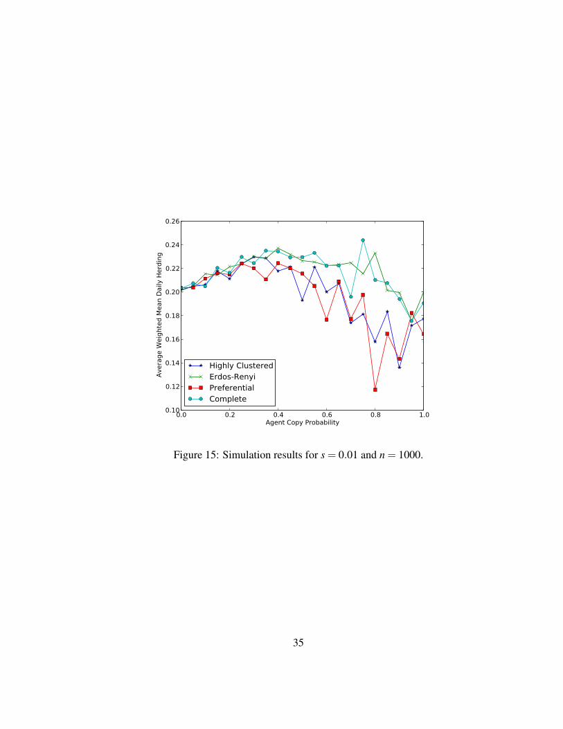
trading thresholds. We now set s = 0.01 for the same two scenarios above. The results of

this set of experiments are shown in figure 15. In these scenarios, where agents

independently adjust their thresholds a small percentage of the time, increasing pcopy to a

certain point increases the overall degree of herding in the system. First, it is interesting to

note that in none of the configurations shown in figure 15 does the value of mean daily

34

0.0 0.2 0.4 0.6 0.8 1.0Agent Copy Probability

0.10

0.12

0.14

0.16

0.18

0.20

0.22

0.24

0.26

Aver

age

Wei

ghte

d M

ean

Daily

Her

ding

Highly ClusteredErdos-RenyiPreferentialComplete

Figure 15: Simulation results for s = 0.01 and n = 1000.

35

herding reach the maximum obtained in figure 14, where s = 0. Similarly, each network

configuration with s = 0.01 maintains an average mean herding value greater than the

minimum obtained from the set of s = 0 experiments.

To summarize:

1. The highest total degree of herding occurs in systems where agents never update

their initial thresholds and rarely copy another agent’s thresholds.

2. In systems where agents do update their thresholds a small percentage of the time,

modest levels of pcopy yield higher herding values than pcopy = 0.

3. Beyond these modest levels, herding begins to decrease, but not as sharply as

systems in which s = 0.

Why does the measure of herding decrease as we increase the propensity for agents to

copy the behavior of other agents in our first set of experiments? Obviously, this is more

of a problem with our measure of investor herding than with the mechanics of our

simulated system. After all, in each set of experiments, we know exactly how much agents

are copying each other - we specify as input to our system that an agent will copy the

behavior of one of her neighbors some number of turns (pcopy) on average.

The counter-intuitive nature of the herding results in these simulations stems from the

fact that we are modeling agent herding behavior on a local level, while the measure of

herding we use aims to capture the degree of herding on a global (system-wide) scale.

Remember, the financial view of herding behavior is investors “flocking” to the same

position as everyone else, regardless of their independent beliefs. Now, the term

“everyone else” is of course fuzzy: does an investor root their herding behavior in their

perception of the actions of a large group of other investors, or in the actions of a few (or

36

single) investors with whom they have direct contact? From the results of our first set

simulation experiments, it would seem that the latter scenario does not necessarily

produce the degree of herding we expect to see on a global scale. It is not until the agents

of our system adjust their independent beliefs by some simple rule (with frequency s) that

our local model of individual investor herding yields increased global herding.

One possible explanation for higher pcopy leading to lower herding when s = 0 is the

following: let I be the instrument which is traded most frequently. If the propensity for

agents to copy their neighbors moves brI (the buy ratio of I) closer to the total buy ratio,

while bri for i 6= I, stays about the same, this would have the effect of decreasing hI , and

thus would decrease H. We can imagine a real-world scenario where the “hottest”

instrument is also the most sensitive in terms of investors’ subjective views (i.e. has the

narrowest threshold range). In this case, imitation behavior would have the greatest effect

on this instrument, and if imitation caused the buy ratio of the instrument to move toward

the total buy ratio, then, by virtue of I being the most popularly traded instrument, total

herding would decrease.

3.3.1 Cranking up s

As we stated earlier, Cont suggested in his model that s take values in the range

10−1−10−3. Having not been convinced that a value of s = 0.01 is particularly

appropriate or realistic for our model, we may examine simulated network models in

which the frequency with which agents update their signal thresholds is increased by

ten-fold to s = 0.1. Again, if we’re drawing a loose correlation to the real world, we’ll

have trading agents that adjust their private views on price volatility once every ten days

37

0.0 0.2 0.4 0.6 0.8 1.0Agent Copy Probability

0.12

0.14

0.16

0.18

0.20

0.22

0.24

0.26

0.28

Aver

age

Wei

ghte

d M

ean

Daily

Her

ding

Highly ClusteredErdos-RenyiPreferentialComplete

Figure 16: Simulations with s = 0.1 and n = 1000.

on average (rather than once every 100 days). We’ll use the same simulation parameters as

used in our first two sets of experiments for s = 0 and s = 0.01.

The outcome of experiments with substantially higher update probability s yields a

dramatically different picture from experiments in which s is small: as the value of pcopy

increases, the average values of mean daily herding increase. In fact, the weighted average

of the mean daily herding measure increases about two-fold as pcopy is incremented in the

preferential attachment network configuration. This is a pleasant surprise at an empirical

level: the expectation of our simplified investor behavior model is that as agents copy the

behavior of their neighbors with greater frequency, the aggregate level of investor herding

will increase. This network model supports our intuition. The only difference in this set of

experiments is a value of s = 0.1, which is ten times greater than the value of s in our

38

previous set of experiments. Qualitatively, this means that, in the context of an individual

agent’s trading behavior, investment strategies are more dynamic. Adjustments to

volatility thresholds are made much more frequently, and they move in a direction

proportional to the most recent return on an instrument. We might say this situation is one

in which agents are more “informed”.

But why should it be the case that a system with more informed agents displays a

higher degree of herding in the presence of more neighbor copying than a system in which

agents are less informed? Perhaps the use of the term “information” here is a misnomer.

Past information on prices is always available to the agents in our model. However, the

frequency with which that price information is used to adjust an agent’s view on volatility

changes according to s. Thus, when s is small, an agent only makes small adjustments to

her views between long intervals of time, whereas when s is comparatively larger, she will

make small adjustments over many short intervals. A higher frequency of threshold

updates will lead each agent to adjust her views such that they are more consistent with

the most recent returns on the prices of instruments. I hypothesize that this is leading to a

narrower range of thresholds among agents, and thus that an increasing propensity for

copying neighbor thresholds is leading to more instances (or opportunities) for an agent

who is a buyer/seller to flip her view on a given day and become a seller/buyer. The idea

here is that since the range of possible threshold values in the system becomes narrower

around the actual price of each instrument, the probability of activating a threshold that

has been copied from a neighbor increases.

39

0.10

0.11

0.12

0.13

0.14

0.15

0.16

Mean D

aily

Herd

ing

100 200 300 400 500 600 700 800 900 1000Number of Nodes

WeightedUnweighted

(a) Average Mean Daily Herding vs. n in a random

network configuration

0.11

0.12

0.13

0.14

0.15

0.16

0.17

Mean D

aily

Herd

ing

100 200 300 400 500 600 700 800 900 1000Number of Nodes

WeightedUnweighted

(b) Average Mean Daily Herding vs. n in a preferen-

tial attachment configuration

Figure 17: Simulation experiment with s = 0.01 and pcopy = 0.1.

3.3.2 Effects of Scale

It’s also interesting to see how this model scales. We present here simulation results with

s = 0.01, pcopy = 0.1 and n varying from 100 to 1000. We observe both an Erdos and

Renyi random network and a preferential attachment network. Notice that the weighted

measure of herding stays somewhat constant, with small fluctuations, while the

unweighted measure increases quickly with the addition of the first few hundred nodes,

before converging to a level commensurate with the weighted measure.

Similarly, we have above the results of a set of experiments in which n is fixed at 100

and m is increased in fixed intervals. We observe the same two network types as before,

and see again small variations but the same basic trend for both the weighted and

unweighted measure.

40

0.10

0.11

0.12

0.13

0.14

0.15

0.16

Mean D

aily

Herd

ing

0.0 0.2 0.4 0.6 0.8 1.0Link Probability

WeightedUnweighted

(a) Average Mean Daily Herding vs. m in a random

network configuration

0.10

0.11

0.12

0.13

0.14

0.15

0.16

Mean D

aily

Herd

ing

0 10 20 30 40 50Number of Edges per New Node

WeightedUnweighted

(b) Average Mean Daily Herding vs. m in a preferen-

tial attachment configuation

Figure 18: Simulation experiment with s = 0.01 and pcopy = 0.1.

3.4 Conclusion

In this chapter, we set out to answer the question “What effect does network topology

have on herding among investors, if any?” From our results, the answer seems to be: not

much 5. It does seem from experiments with s = 0 and s = 0.01 that complete networks

and networks formed according to the random graph process of Erdos and Renyi generally

exhibit herding values slightly higher than tightly clustered networks. However, these

values of s do not jibe particularly well with our notion of how herding values should look

with respect to individuals’ copying behavior. When we increase the update frequency to

s = 0.1 in order adjust for this fact, we get results that are similarly erratic, although

consistent in their upward trend.

5Or more generously, to be determined.

41

From these simulations, we might take away the following: when agents are less

informed (or when they make little or no use of information in adjusting their subjective

views on volatility), it seems that complete graphs and classical random graphs tend to

have higher degrees of herding than preferentially attached graphs when the frequency of

imitation exceeds a certain threshold (which is about pcopy = 0.4 in our results). However,

in order for the system to behave in aggregate as we would expect (that is, to get increased

herding with increased behavior imitation), it is required that agents make more frequent

adjustments to their investment thresholds based on past results. So, it seems that a system

with better informed agents yields a system in which an increased prevelance of behavior

imitation leads to a higher measure of herding.

42

SIMULATION IMPLEMENTATION

The implemenation of the trading network simulation was discussed briefly in Chapter 3.

Below is a detailed diagram of this implemenation. There are a few details of the

implemenation not discussed above:

1. The OrderBook class holds all of the orders placed for a given simulation. The

TradingNetworkModel (the main Simulation class) is composed in part of an

OrderBook, and at the conclusion of a simulation run, the HerdingAnalysis class

accesses the order book to do the herding computations.

2. A TraderSource object is used to generate Trader (agent) objects that in turn join a

graph. Traders are generated at some random interval. The TraderSource also

passes along the threshold distribution parameters to use in composing an agent’s

volatility thresholds.

3. The main actions of a Trader are to join the network and continuously execute their

strategy during each period of the simulation. Also, the methods getInfected and

getHealthy manage the threshold copying behavior of a given agent.

43

Figu

re19

:Im

plem

enat

ion

ofth

eTr

adin

gN

etw

ork

Sim

ulat

ion.

44

REFERENCE LIST

[ABA03] Lada A. Adamic, Orkut Buyukkokten, and Eytan Adar. A social networkcaught in the web. First Monday, 2003.

[BA99] Albert-Lszl Barabsi and Rka Albert. Emergence of scaling in randomnetworks. Science, 286(5439):509–512, 1999.

[CKE+08] H. Chun, H. Kwak, Y.H. Eom, Y.Y. Ahn, S. Moon, and H. Jeong.Comparison of online social relations in volumevs interaction: a case studyof cyworld. In Proc. of Internet Measurement Conference, 2008.

[Con01] Rama Cont. Empirical properties of asset returns: stylized facts andstatistical issues. Quantitative Finance, 1:223–236, 2001.

[Con07] Rama Cont. Volatility clustering in financial markets: Empirical facts andagent based models. In A. Krman and G. Teyssiere, editors, Long Memory inEconomics, pages 289–310. Springer, 2007.

[CSN09] Aaron Clauset, Cosma Rohilla Shalizi, and M. E. J. Newman. Power-lawdistributions in empirical data. 51(4):661–703, 2009.

[DNT12] Alex Dusenbery, Khahn Nguyen, and Duc A. Tran. Analysis of aninvestment social network. In In Proc. of the IEEE International Conferenceon Communications (ICC2012), Ottawa, Canada, June 2012.

[ER59] P. Erdos and A. Renyi. On random graphs. Publicationes Mathematicae,6:290–297, 1959.

[GCN05] Franois Ghoulmie, Rama Cont, and Jean-Pierre Nadal. Heterogeneity andfeedback in an agent-based market model. Journal of Physics: CondensedMatter, 17(14):S1259, 2005.

[HK02] Petter Holme and Beom Jun Kim. Growing scale-free networks with tunableclustering. Phys. Rev. E, 65:026107, Jan 2002.

[HS01] Soosung Hwang and Mark Salmon. A new measure of herding and empiricalevidence. Warwick Business School, Financial Econometrics ResearchCentre, Coventry, 2001.

[HSS08] Aric A. Hagberg, Daniel A. Schult, and Pieter J. Swart. Exploring networkstructure, dynamics, and function using NetworkX. In Proceedings of the 7thPython in Science Conference (SciPy2008), pages 11–15, Pasadena, CAUSA, August 2008.

45

[JOP+ ] Eric Jones, Travis Oliphant, Pearu Peterson, et al. SciPy: Open sourcescientific tools for Python, 2001–.

[Kre10] Stephanie Kremer. Herding of Institutional Traders. SFB 649 DiscussionPaper 2010-025, Sonderforschungsbereich 649, Humboldt Universitat zuBerlin, Germany, 2010. available athttp://sfb649.wiwi.hu-berlin.de/papers/pdf/SFB649DP2010-025.pdf.

[LeB06] Blake LeBaron. Agent-based computational finance. In L. Tesfatsion andK. Judd, editors, Handbook of Computational Economics, Volume 2:Agent-Based Computational Economics, pages 1187–1232. North-Holland,2006.

[LH08] Jure Leskovec and Eric Horvitz. Planetary-scale views on a largeinstant-messaging network. In Proc. of the International World Wide WebConference, Beijing, China, 2008.

[LS07] Julio Lobao and Ana Paula Serra. Herding behavior: Evidence fromportuguese mutual funds. In Greg N. Gregoriou, editor, Diversification andPortfolio Management of Mutual Funds, pages 167–197. PalgraveMacMillan, New York, 2007.

[LSV92] Josef Lakonishok, Andrei Shleifer, and Robert W. Vishny. The impact ofinstitutional trading on stock prices. Journal of Financial Economics,32(1):23 – 43, 1992.

[LV00] Ignacio N. Lobato and Carlos Velasco. Long memory in stock-markettrading volume. Journal of Business and Economic Statistics,18(4):410–427, 2000.

[Man63] Benoit Mandelbrot. The variation of certain speculative prices. The Journalof Business, 36(4):394–419, 1963.

[MGD06] A. Mislove, K. P. Gummadi, and P. Druschel. Exploiting social networks forinternet search. In Proc. of HotNets, 2006.

[MKG+08] Alan Mislove, Hema Swetha Koppula, Krishna P. Gummadi, Peter Druschel,and Bobby Bhattacharjee. Growth of the flickr social network. In Proc. ofWOSN, 2008.

[MMG+07] Alan Mislove, Massilmiliano Marcon, Krishna P. Gummadi, Peter Druschel,and Bobby Bhattacharjee. Measurement and analysis of online socialnetworks. Proceedings of the 5th ACM/USENIX Internet MeasurementConference, 2007.

46

[MV03] Klaus Muller and Tony Vignaux. SimPy simulation package.http://simpy.sourceforge.net/, 2003.

[New02] M. E. J. Newman. Assortative mixing in networks. Phys. Rev. Lett.,89:208701, Oct 2002.

[New03] M. E. J. Newman. Mixing patterns in networks. Phys. Rev. E, 67:026126,Feb 2003.

[NT09] Khahn Nguyen and Duc A. Tran. An analysis of facebook activities. InProceedings of IEEE Consumer Communications and NetworkingConference (CCNC 2011), 2009.

[VMCG09] Bimal Viswanath, Alan Mislove, Meeyoung Cha, and Krishna P. Gummadi.On the evolution of user interaction in facebook. Proceedings of the 2ndACM SIGCOMM Workshop on Social Networks, 2009.

[Wha09] Robert E. Whaley. Understanding the vix. The Journal of PortfolioManagement, 2009.

[WS98] D. J. Watts and S. H. Strogatz. Collective dynamics of ‘small-world’networks. Nature, 393:440–442, June 1998.

47