Measurements of fluctuation in drag acting on rigid cylinder array in open channel flow

Measurements of fluctuation in drag acting on rigid cylinder array in open 1

channel flow 2

Kuifeng Zhao1; Nian‐Sheng Cheng2; Xikun Wang3; and Soon Keat Tan4 3

1Research Student, School of Civil and Environmental Engineering, Nanyang Technological 4

University, Nanyang Avenue, Singapore 639798. Email: [email protected] 5

2Associate Professor, School of Civil and Environmental Engineering, Nanyang Technological 6


3Senior Research Fellow, Maritime Research Centre, Nanyang Technological University, 8

Nanyang Avenue, Singapore 639798. Email: [email protected] 9

4Associate Professor, School of Civil and Environmental Engineering, Nanyang Technological 10


12

Abstract 13

In this study, an array of rigid cylindrical rods was used to simulate emergent vegetation 14

stems that were subject to unidirectional open channel flows. The instantaneous drag force 15

experienced by the rods was measured with a load cell. In addition, Particle Image 16

Velocimetry (PIV) technique was applied to sample the flow information in a horizontal 17

plane and wave gauges were used to record the fluctuation in the water‐surface elevation. 18

The results show that the drag fluctuation normalized by the mean value may reach as high 19

as 133% when the Reynolds number (defined based on the stem diameter) varied in the 20

range from 400 to 1100. High fluctuations were also observed in the flow velocity and flow 21

depth under similar flow conditions. 22

23

Introduction 24

In the past decades, various laboratory experiments have been conducted to study 25

characteristics of open channel flows subject to submerged or emergent vegetation 26

(Kouwen et al. 1969; Nepf 1999; Ishikawa et al. 2000; James et al. 2004; Järvelä 2004; 27

Wilson et al. 2008; Wu 2008; Kothyari et al. 2009; Yang and Choi 2010; Cheng and Nguyen 28

2011). In these studies, an array of rigid cylinders was often adopted to represent the stem 29

or trunk of vegetation. In particular, the understanding of flow characteristics around rigid 30

cylinders provides basis for analysis of flow resistance in vegetated channels (Stone and 31

Shen 2002). Most of the previous studies focused only on the measurement of mean flow 32

velocity and channel resistance. In comparison, only few efforts have been reported to 33

directly measure the drag acting on the vegetation (Ishikawa et al. 2000; Thompson et al. 34

2004; Kothyari et al. 2009; Tinoco and Cowen 2013). 35

Ishikawa et al. (2000) measured the mean drag acting on emergent cylinders using a 36

strain gauge. Their study yielded that the drag coefficient (CD) is related to the ratio of the 37

mean flow velocity to the shear velocity, channel slope, as well as the vegetation density 38

defined as the fraction of the bed area occupied by the vegetation. Kothyari et al. (2009) 39

also measured the mean drag force using a strain gauge but expressed CD as a function of 40

the Reynolds number (RD, which was defined based on the cylinder diameter and vegetation 41

density). They observed that CD was constant for the subcritical flow and rapidly decreased 42

for the supercritical flow. Tinoco and Cowen (2013) used a drag plate to measure the drag 43

acting on both a single cylinder and an array of cylinders. They found a quadratic 44

relationship between the drag and velocity, and the drag coefficient varied between 1.5 and 45

2 with the Reynolds numbers ranging from 60 to 4550. 46

Due to vortex shedding, significant fluctuations could be observed in the force 47

experienced by the cylinders, relevant flow velocities and flow depth. For example, the 48

maximum fluctuation in the flow depth could reach about 40% of the mean flow depth, as 49

reported by Zima and Ackermann (2002) and Ghomeshi et al. (2007). Similar fluctuations 50

could also occur in the drag, but they have not been investigated in detail. In particular, it is 51

not clear how fluctuations in different variables (i.e., force, velocity and flow depth) are 52

related to one another. Therefore, the main objective of this study is to provide a relatively 53

systematic measurement of the flow through an array of emergent rigid cylinders in an open 54

channel, based on which the correlation between these flow variables could be explored. 55

In this study, a load cell was used to measure the mean drag and its fluctuation 56

experienced by an array of rigid cylinders in open channel flows. In addition, variations in 57

flow velocity and flow depth were sampled under similar flow conditions. The experimental 58

results show that all the fluctuations vary consistently with the Reynolds number. 59

60

Experimental Setup 61

Experiments were conducted with two flumes (Flume A and Flume B), of which the 62

information is summarized in Table 1. Rigid Perspex cylinders (11.00 cm in length and 0.83 63

cm in diameter) were used to simulate vegetation. They were fixed into precisely machined 64

holes on Perspex plates, each being 1.20 m long, 0.30 m wide, and 0.01 m thick. Three 65

different spacings (0.03, 0.06, and 0.09 m) were applied to arrange the cylinders in 66

staggered pattern to mimic different densities of vegetations (Cheng and Nguyen 2011). The 67

three types of configurations are denoted as C30, C60 and C90. The vegetation densities (λ), 68

defined as the percentage bed area occupied by vegetation, were calculated from the 69

geometry of the pattern and they were 12.0%, 3.0% and 1.3% respectively. The 70

configurations C60 and C90 are considered to be sparse while that of C30 is dense, 71

according to the classification given by Nepf (1999). The length covered by vegetation was 72

3.90 m in Flume A and 6.00 m in Flume B. Different runs of tests were completed for 73

configurations C30, C60 and C90; they were 20, 35 and 33, respectively, for Flume A, and 5, 74

20 and 9 for Flume B. Flow meters (accurate to 0.01 L/s) were used for recording flowrate 75

and the cross‐sectional averaged values are denoted as Qmean. All the experiments were 76

conducted under uniform flow conditions. For each test, a uniform flow was achieved by 77

adjusting the bed slope, tailgate and flowrate, so that the flow depths at four different 78

locations along the channel vegetation zone were equal to each other. Mean flow depth 79

(hmean) ranged from 6.30 cm to 9.70 cm, flow rate (Qmean) from 0.65 L/s to 4.55 L/s, and 80

channel slope from 0.0004 to 0.0102. The average pore velocity through the cylinders was 81

then calculated as )]1(/[ λ−= meanmeanVmean BhQV , where B is channel width. The diameter (d) 82

based Reynolds number (RD) was calculated as d/νV= VmeanDR , where ν is the kinematic 83

viscosity of fluid, and the Froude number was calculated as meanVmean ghV / , where g is the 84

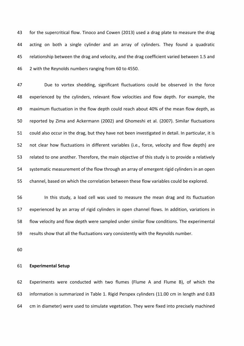
gravitational acceleration. The test sections were selected to be at least 12hmean away, 85

according to Liu et al. (2008), from the upstream edge of the vegetation zone to ensure that 86

the flow was fully developed. 87

Flume A was used to conduct measurements of drag forces and flow velocities. An 88

illustrative sketch of the experimental system is shown in Fig. 1 (a) and (b). The bottom and 89

sidewalls were made of glass to enable optical access. The drag and lateral forces acting on 90

the cylinders were recorded with a three‐component piezoelectric load cell (Kistler Model 91

9317B). This type of load cell has the advantage of high response and high resolution and 92

hence has been widely used (e.g., Lam et al. 2003). The load cell was installed on a special 93

plate that was 0.30 m long 0.30 m wide and 0.01 m thick. The center of the special plate 94

[see Fig. 1 (b)] was 2.55 m from the upstream edge of the vegetation zone, and 1.80 m from 95

tailgate. Inserted on the plate were transparent Perspex cylinders (11.00 cm in length and 96

8.00 cm in diameter), which were arranged in the same pattern as those downstream and 97

upstream of the test section. All the transparent cylinders were installed vertically in a 98

cantilever manner with a clearance of 0.20 cm between the lower ends of the cylinders and 99

the channel bed. This cantilever arrangement avoided the load cell from being submerged in 100

water. 101

For the vegetation configuration employed, the drag acting on the cylinder rods are 102

considered dominant in comparison with the bed and sidewall friction. This is explained as 103

follows. In most of the cases, the average drag coefficient can be approximated as a 104

constant (close to 1.0), according to Cheng and Nguyen (2011) who investigated vegetation 105

resistance with similar vegetation configurations. Therefore, the average drag is 106

proportional to the square of the velocity through the cylinders. On the other hand, it has 107

been found that the flow velocity (streamwise) through the rods is largely uniform in the 108

majority of the flow depth and decreases to zero only near the bed (Nepf et al. 1998; Liu et 109

al. 2008; Cheng and Nguyen 2011; Cheng et al. 2012). As a result, the bed effect on the drag 110

is negligible. This has been verified by experimental data, for example, the drag partition 111

conducted by Cheng and Nguyen (2011) for open channel flows subject to emergent 112

vegetation. 113

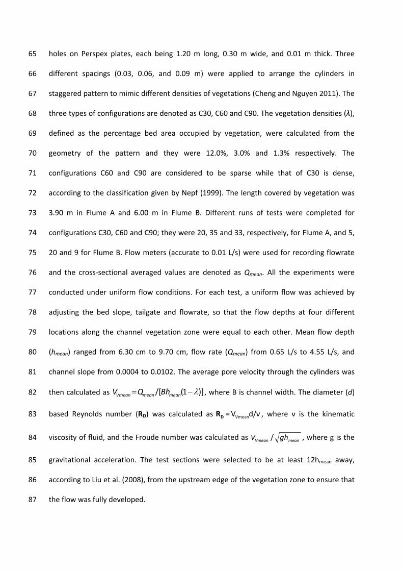
The force measurement setup was calibrated in‐situ against a reference sensor. The 114

point of action of the drag on average varied from 3.20 cm to 4.90 cm (when hmean = 6.30 115

cm‐9.70 cm) from the lower end of the cylinders. With the reference sensor, a reference 116

force in the streamwise or lateral direction (denoted as FX and FY, respectively), was first 117

applied on a cylinder at 3.00 cm and 4.50 cm from the end of the cylinder. Then the induced 118

force (i.e. output) was recorded with the load cell. A comparison of the reference force and 119

the recorded force is presented in Fig. 2 (a), showing that the recorded force is equal to 95% 120

of the reference force. The calibration result also shows that the load cell could record the 121

forces well regardless of the point at which the force acts. 122

The reason for involving multiple cylinders in the measurement of the drag is that 123

the force experienced by a single cylinder was beyond the recordable range to response 124

correctly. The load cell was connected with a signal amplifier controlled by a computer. The 125

output signal was then captured with a data acquisition card (National Instruments) at a 126

sampling rate of 1K Hz. To verify whether the load cell is accurately responsive to low 127

frequency signals, a separate dynamic response test was also conducted with reference to a 128

strain gauge. First, a reference (i.e. input) signal was recorded using a strain gauge sensor, 129

which is suitable for the measurement of low‐frequency response. The generated forces, FX 130

and FY, were quasi‐periodic, varying with a frequency of about 1 Hz. Then the induced force 131

(i.e. output) was measured using the load cell. Fig. 2 (b) and (c) show the results of the input 132

signals, in comparison with the output signals measured by the load cell. It can be seen that 133

the agreement between the input and output signals is excellent, which validated the force 134

measurement system employed in the experiments. To obtain meaningful statistics of the 135

measured data, a plot of probability density function (pdf) of the recorded force with the 136

sampling duration of 1 s, 40 s, 80 s and 120 s is shown in Fig. 3 for illustration. As the 137

duration increases up to 40 s, 80 s and 120 s, the statistics values (the mean value and 138

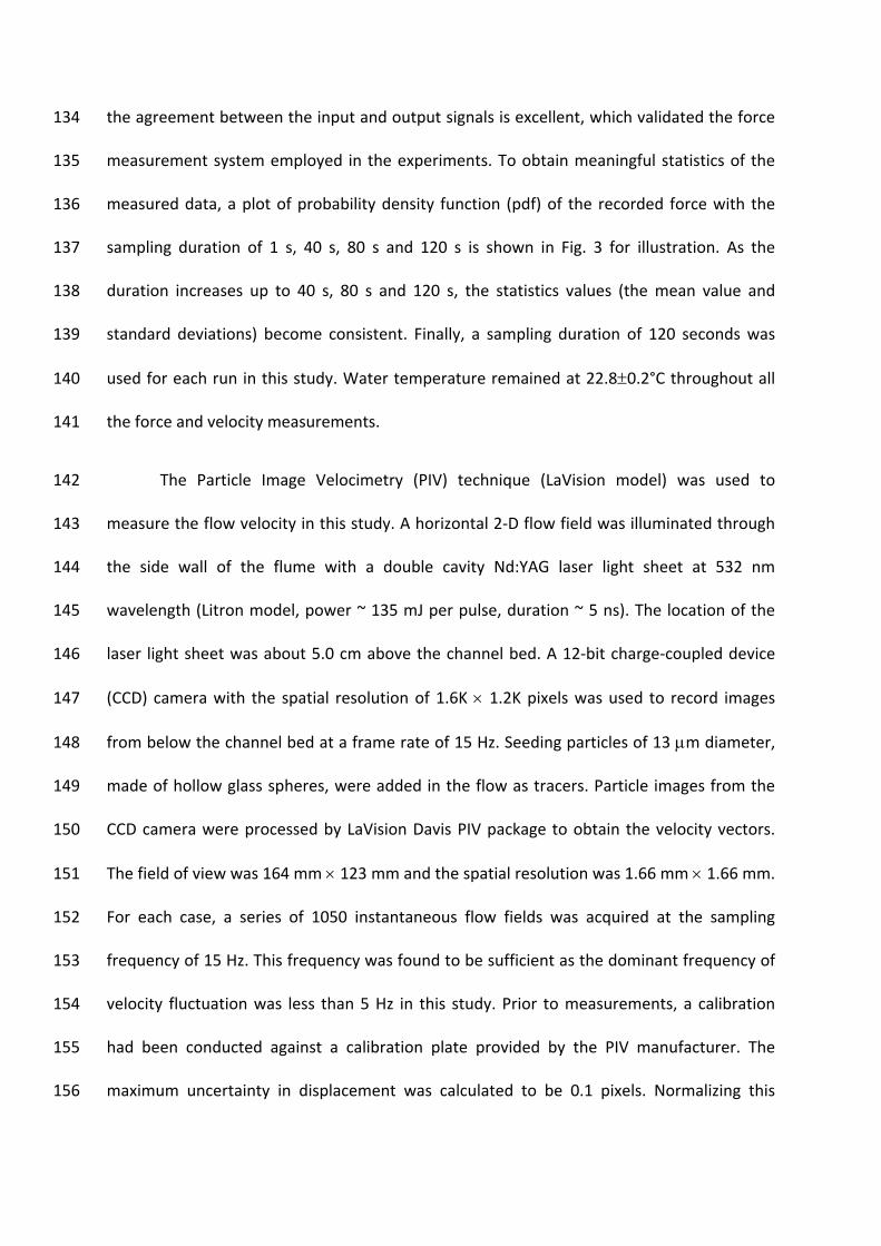
standard deviations) become consistent. Finally, a sampling duration of 120 seconds was 139

used for each run in this study. Water temperature remained at 22.8±0.2°C throughout all 140

the force and velocity measurements. 141

The Particle Image Velocimetry (PIV) technique (LaVision model) was used to 142

measure the flow velocity in this study. A horizontal 2‐D flow field was illuminated through 143

the side wall of the flume with a double cavity Nd:YAG laser light sheet at 532 nm 144

wavelength (Litron model, power ~ 135 mJ per pulse, duration ~ 5 ns). The location of the 145

laser light sheet was about 5.0 cm above the channel bed. A 12‐bit charge‐coupled device 146

(CCD) camera with the spatial resolution of 1.6K × 1.2K pixels was used to record images 147

from below the channel bed at a frame rate of 15 Hz. Seeding particles of 13 μm diameter, 148

made of hollow glass spheres, were added in the flow as tracers. Particle images from the 149

CCD camera were processed by LaVision Davis PIV package to obtain the velocity vectors. 150

The field of view was 164 mm × 123 mm and the spatial resolution was 1.66 mm × 1.66 mm. 151

For each case, a series of 1050 instantaneous flow fields was acquired at the sampling 152

frequency of 15 Hz. This frequency was found to be sufficient as the dominant frequency of 153

velocity fluctuation was less than 5 Hz in this study. Prior to measurements, a calibration 154

had been conducted against a calibration plate provided by the PIV manufacturer. The 155

maximum uncertainty in displacement was calculated to be 0.1 pixels. Normalizing this 156

uncertainty with the mean displacement of the particles (about 5 pixels) yielded a relative 157

error of 2% for the instantaneous streamwise and transverse velocities (u and v). A detailed 158

description of the PIV post‐processing procedure and uncertainty analysis is available in 159

Wang and Tan (2008). 160

Fig. 4 shows a representative snapshot of the PIV images and the coordinate system 161

used, in which water flows from left to right. The square is the area selected for analysis 162

because it is the central area which had the least blockage of light. Four circles represent the 163

positions of the four cylinders. The spacing is defined as the center‐to‐center distance 164

between two neighbouring cylinders. The origin of the coordinate was located at the centre 165

of the upstream cylinder. When the laser was emitted from the side of the flume, some 166

cylinders, though transparent, affected the laser so that the PIV results in the shaded 167

rectangular area were of poor quality and thus excluded for the analysis. The dominant 168

frequency of lateral velocity fluctuation was calculated by applying FFT analysis to the v 169

component that was measured at the points about 1.5d downstream of cylinders on the 170

wake axis. 171

It should be mentioned that because of unavailability of wave gauges, we could not 172

measure the fluctuation in the flow depth at the same time when conducting drag and flow 173

measurements with Flume A. Then Flume B [see sketch in Fig. 1 (c)], which was 12.00 m long 174

and 0.30 m wide, was used to conduct supplementary tests for measuring the fluctuation in 175

the flow depth. In the supplementary tests, the flow condition including the channel slope, 176

flowrate and flow depth was made comparable to that in Flume A (see Table 1). With similar 177

flow conditions and vegetation configurations, the use of the two flumes does not affect the 178

statistical results, e.g. rms values, varying with the Reynolds number, as presented later in 179

this paper. The wave gauges of the resistance type, comprising of three probes, were 180

installed at the test section, which was 3.00 m (i.e. over 30 times the flow depth) from the 181

upstream edge of the vegetation zone and 4.00 m from the tailgate. Each probe had two 182

pieces of parallel metal sticks which was able to conduct electricity when submerged in 183

water. The two sticks, 1.00 cm apart, formed a plane that was aligned with the sidewall. The 184

planes associated with the three probes were located at a distance 1.90 cm, 11.60 cm and 185

26.30 cm from one sidewall of the flume. The locations were selected to observe the 186

maximum fluctuation of the flow depth that may appear at different points across the y 187

direction. The probes were connected with an amplifier to increase the output level of 188

voltage signals and further connected to a computer for recording. DEWESoft data 189

acquisition device was used to take recordings at a frequency of 100 samples per second. 190

The probes were calibrated in still water before pump was turned on. 191

192

Data Analysis 193

With the time averaged drag, FDmean, acting on the cylindrical stems, the time averaged drag 194

coefficient (CDmean) is defined as 195

2Vmeanmean

DmeanDmean Vρdh

FC

2= (1)

where ρ is the fluid density. By normalizing the drag fluctuation FD' in the same way as 196

shown in Eq. (1), the fluctuation in the drag coefficient (CD') can be expressed as 197

(Gopalkrishnan 1993; Sumer and Fredsøe 2006), 198

2

'2'

Vmeanmean

DD Vdh

FC

ρ= (2)

where the superscript prime ( ' ) denotes the instantaneous fluctuations. Using Eqs (1) and 199

(2), one gets 200

Dmean

Drms

Dmean

Drms

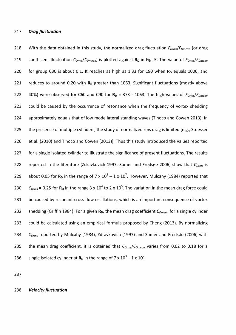
F

F

C

C= (3)

where 2'DDrms CC = and 2'DDrms FF = are the root‐mean‐square (rms) values. The other rms 201

variables of interest include hrms used for quantifying flow depth fluctuations, and urms and 202

vrms for quantifying streamwise and lateral velocity fluctuations. The variations of FDrms, CDrms, 203

hrms and urms with flow conditions are discussed in the following sections. The relationship 204

among the various rms parameters is also of the authors’ interest; however it cannot be 205

fully explored in this study as the experiments were conducted in two flumes. 206

207

Results 208

Reynolds number serves as an important parameter to study the variation of the drag acting 209

on an isolated cylinder (Kundu and Cohen 2002). Similar variations and the Reynolds 210

number dependence could be expected in the presence of the cylinder array as considered 211

in this study. To characterize the flow through the cylinders, the average pore velocity 212

(VVmean) is used to define the Reynolds number as RD = VVmeand/ν. In the following, variations 213

of the normalized parameters including FDrms/FDmean, urms/VVmean and hrms/hmean with RD are 214

examined. 215

216

Drag fluctuation 217

With the data obtained in this study, the normalized drag fluctuation FDrms/FDmean (or drag 218

coefficient fluctuation CDrms/CDmean) is plotted against RD in Fig. 5. The value of FDrms/FDmean 219

for group C30 is about 0.1. It reaches as high as 1.33 for C90 when RD equals 1006, and 220

reduces to around 0.20 with RD greater than 1063. Significant fluctuations (mostly above 221

40%) were observed for C60 and C90 for RD = 373 ‐ 1063. The high values of FDrms/FDmean 222

could be caused by the occurrence of resonance when the frequency of vortex shedding 223

approximately equals that of low mode lateral standing waves (Tinoco and Cowen 2013). In 224

the presence of multiple cylinders, the study of normalized rms drag is limited [e.g., Stoesser 225

et al. (2010) and Tinoco and Cowen (2013)]. Thus this study introduced the values reported 226

for a single isolated cylinder to illustrate the significance of present fluctuations. The results 227

reported in the literature (Zdravkovich 1997; Sumer and Fredsøe 2006) show that CDrms is 228

about 0.05 for RD in the range of 7 x 103 – 1 x 107. However, Mulcahy (1984) reported that 229

CDrms = 0.25 for RD in the range 3 x 104 to 2 x 105. The variation in the mean drag force could 230

be caused by resonant cross flow oscillations, which is an important consequence of vortex 231

shedding (Griffin 1984). For a given RD, the mean drag coefficient CDmean for a single cylinder 232

could be calculated using an empirical formula proposed by Cheng (2013). By normalizing 233

CDrms reported by Mulcahy (1984), Zdravkovich (1997) and Sumer and Fredsøe (2006) with 234

the mean drag coefficient, it is obtained that CDrms/CDmean varies from 0.02 to 0.18 for a 235

single isolated cylinder at RD in the range of 7 x 103 – 1 x 107. 236

237

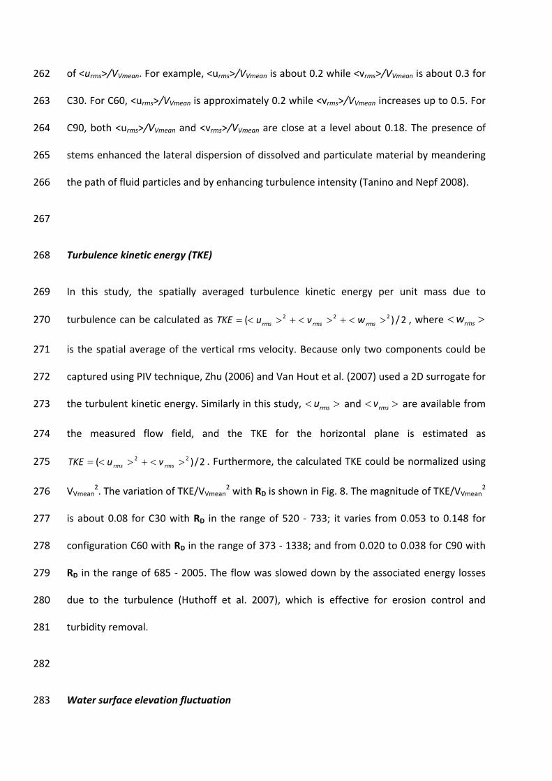
Velocity fluctuation 238

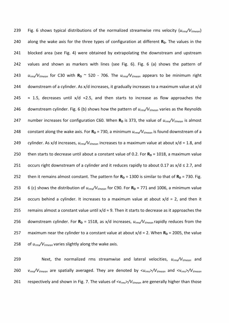
Fig. 6 shows typical distributions of the normalized streamwise rms velocity (urms/VVmean) 239

along the wake axis for the three types of configuration at different RD. The values in the 240

blocked area (see Fig. 4) were obtained by extrapolating the downstream and upstream 241

values and shown as markers with lines (see Fig. 6). Fig. 6 (a) shows the pattern of 242

urms/VVmean for C30 with RD ~ 520 ‐ 706. The urms/VVmean appears to be minimum right 243

downstream of a cylinder. As x/d increases, it gradually increases to a maximum value at x/d 244

≈ 1.5, decreases until x/d ≈2.5, and then starts to increase as flow approaches the 245

downstream cylinder. Fig. 6 (b) shows how the pattern of urms/VVmean varies as the Reynolds 246

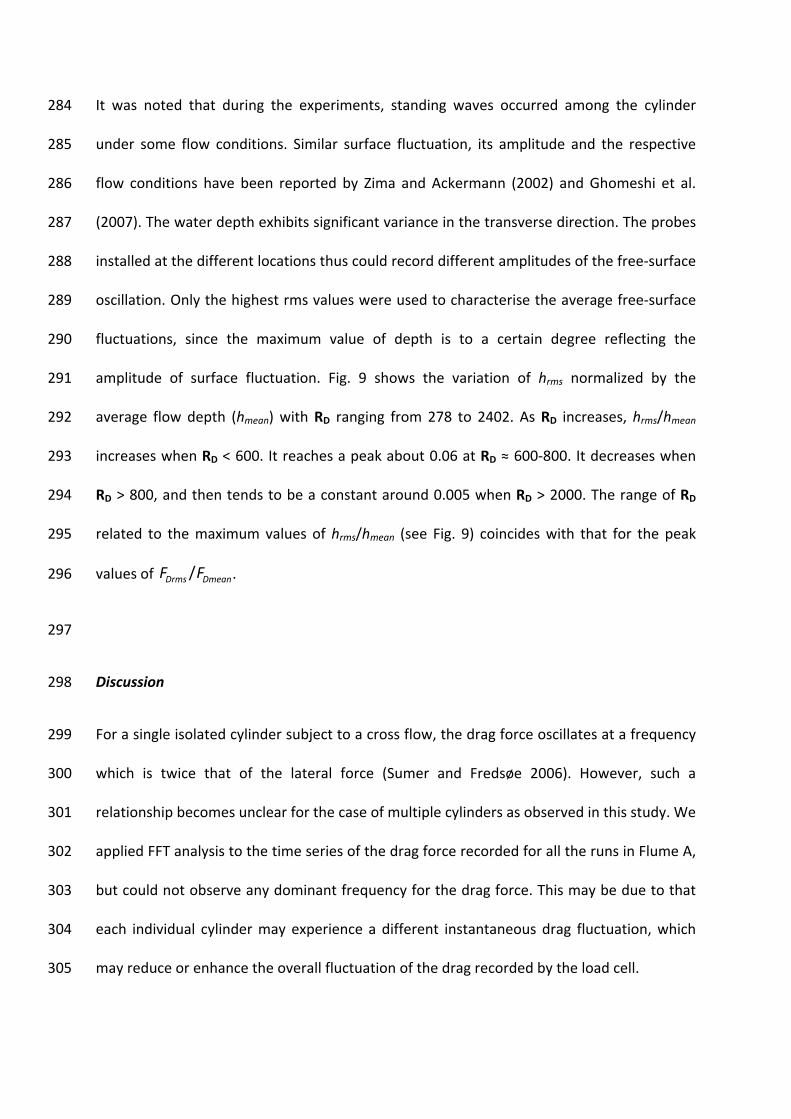
number increases for configuration C60. When RD is 373, the value of urms/VVmean is almost 247

constant along the wake axis. For RD = 730, a minimum urms/VVmean is found downstream of a 248

cylinder. As x/d increases, urms/VVmean increases to a maximum value at about x/d = 1.8, and 249

then starts to decrease until about a constant value of 0.2. For RD = 1018, a maximum value 250

occurs right downstream of a cylinder and it reduces rapidly to about 0.17 as x/d ≤ 2.7, and 251

then it remains almost constant. The pattern for RD = 1300 is similar to that of RD = 730. Fig. 252

6 (c) shows the distribution of urms/VVmean for C90. For RD = 771 and 1006, a minimum value 253

occurs behind a cylinder. It increases to a maximum value at about x/d = 2, and then it 254

remains almost a constant value until x/d ≈ 9. Then it starts to decrease as it approaches the 255

downstream cylinder. For RD = 1518, as x/d increases, urms/VVmean rapidly reduces from the 256

maximum near the cylinder to a constant value at about x/d = 2. When RD = 2005, the value 257

of urms/VVmean varies slightly along the wake axis. 258

Next, the normalized rms streamwise and lateral velocities, urms/VVmean and 259

vrms/VVmean are spatially averaged. They are denoted by <urms>/VVmean and <vrms>/VVmean 260

respectively and shown in Fig. 7. The values of <vrms>/VVmean are generally higher than those 261

of <urms>/VVmean. For example, <urms>/VVmean is about 0.2 while <vrms>/VVmean is about 0.3 for 262

C30. For C60, <urms>/VVmean is approximately 0.2 while <vrms>/VVmean increases up to 0.5. For 263

C90, both <urms>/VVmean and <vrms>/VVmean are close at a level about 0.18. The presence of 264

stems enhanced the lateral dispersion of dissolved and particulate material by meandering 265

the path of fluid particles and by enhancing turbulence intensity (Tanino and Nepf 2008). 266

267

Turbulence kinetic energy (TKE) 268

In this study, the spatially averaged turbulence kinetic energy per unit mass due to 269

turbulence can be calculated as 2/)( 222 ><+><+><= rmsrmsrms wvuTKE , where >< rmsw 270

is the spatial average of the vertical rms velocity. Because only two components could be 271

captured using PIV technique, Zhu (2006) and Van Hout et al. (2007) used a 2D surrogate for 272

the turbulent kinetic energy. Similarly in this study, >< rmsu and >< rmsv are available from 273

the measured flow field, and the TKE for the horizontal plane is estimated as 274

2/)( 22 ><+><= rmsrms vuTKE . Furthermore, the calculated TKE could be normalized using 275

VVmean2. The variation of TKE/VVmean

2 with RD is shown in Fig. 8. The magnitude of TKE/VVmean2 276

is about 0.08 for C30 with RD in the range of 520 ‐ 733; it varies from 0.053 to 0.148 for 277

configuration C60 with RD in the range of 373 ‐ 1338; and from 0.020 to 0.038 for C90 with 278

RD in the range of 685 ‐ 2005. The flow was slowed down by the associated energy losses 279

due to the turbulence (Huthoff et al. 2007), which is effective for erosion control and 280

turbidity removal. 281

282

Water surface elevation fluctuation 283

It was noted that during the experiments, standing waves occurred among the cylinder 284

under some flow conditions. Similar surface fluctuation, its amplitude and the respective 285

flow conditions have been reported by Zima and Ackermann (2002) and Ghomeshi et al. 286

(2007). The water depth exhibits significant variance in the transverse direction. The probes 287

installed at the different locations thus could record different amplitudes of the free‐surface 288

oscillation. Only the highest rms values were used to characterise the average free‐surface 289

fluctuations, since the maximum value of depth is to a certain degree reflecting the 290

amplitude of surface fluctuation. Fig. 9 shows the variation of hrms normalized by the 291

average flow depth (hmean) with RD ranging from 278 to 2402. As RD increases, hrms/hmean 292

increases when RD < 600. It reaches a peak about 0.06 at RD ≈ 600‐800. It decreases when 293

RD > 800, and then tends to be a constant around 0.005 when RD > 2000. The range of RD 294

related to the maximum values of hrms/hmean (see Fig. 9) coincides with that for the peak 295

values of DmeanDrms FF / . 296

297

Discussion 298

For a single isolated cylinder subject to a cross flow, the drag force oscillates at a frequency 299

which is twice that of the lateral force (Sumer and Fredsøe 2006). However, such a 300

relationship becomes unclear for the case of multiple cylinders as observed in this study. We 301

applied FFT analysis to the time series of the drag force recorded for all the runs in Flume A, 302

but could not observe any dominant frequency for the drag force. This may be due to that 303

each individual cylinder may experience a different instantaneous drag fluctuation, which 304

may reduce or enhance the overall fluctuation of the drag recorded by the load cell. 305

The fluctuation of the lateral velocity is believed to be closely related to that of the 306

lateral force and water surface elevation. To further understand how different fluctuating 307

variables are related to each other, FFT techniques were applied to obtain the dominant 308

frequency. For the tests conducted in Flume A, dominant frequencies (f) were clearly found 309

for both the lateral force and lateral velocity for 44 runs. Similarly, we also found dominant 310

frequencies for the water surface fluctuation for 27 runs of all the tests conducted in Flume 311

B. The results expressed in terms of Strouhal number (St=fd/VVmean) are shown in Fig. 10. It 312

seems that the normalized frequencies, though derived from the different time series, vary 313

with RD in a similar fashion. The value of St first decreases with increasing RD when RD < 600, 314

and then increases when RD = 600 – 800. It finally decreases to about 0.2 when RD > 1000. In 315

particular, it is noted that the variation of St has a transition at the Reynolds numbers 316

ranging from 600 to 800. This is exactly the range where the maximum fluctuation occurs in 317

the drag, velocity and flow depth. This affirms that the periodical and amplified fluctuation 318

is strongly related with the vortex shedding. Further efforts should be made to explore flow 319

phenomena including the vortex shedding and surface waves in the transition. These 320

oscillations in water depth, velocity and turbulence have potential to create morphological 321

features and improve fish habitat (Sadeque et al. 2009). 322

323

Conclusions 324

This study investigated the mean drag and its fluctuation that was experienced by an array 325

of emergent rigid cylinders in an open channel flow. The rms drag was found to be 326

significant (up to 133% of the mean drag) for the Reynolds number in the range of 400‐1100. 327

The drag fluctuation was closely related to the flow velocity, the flow depth and their 328

fluctuations. The observations show that high fluctuations also occur in the flow velocity 329

and flow depth for the Reynolds number of the same range. Finally, the data analysis yields 330

that consistent variations in the dominant frequency can be derived from the measured 331

fluctuations in the lateral force, lateral velocity and flow depth. 332

333

List of Symbols 334

CD = instantaneous drag coefficient

CDmean = average drag coefficient

CD' = drag coefficient fluctuation

CDrms = rms of CD'

d = cylinder diameter

f = frequency

FD = instantaneous drag

FDmean = average drag

FD' = drag fluctuation

FDrms = rms of FD'

FX = force on cylinder in x direction

FY = force on cylinder in y direction

h = instantaneous flow depth

hmean = average flow depth

h' = flow depth fluctuation

hrms = rms of 'h

Qmean = average flowrate

RD = cylinder Reynolds number = VVmeand/ν

S = channel bed slope

St = Strouhal number

umean = time‐mean streamwise velocity

urms = rms of streamwise velocity fluctuation

<urms> = spatially averaged rmsu

<vrms> = spatially averaged vrms

VVmean = average pore velocity, [ ])1(/ λ−meanmean BhQ

<wrms> = spatially averaged wrms

x = longitudinal direction

y = transverse direction

λ = vegetation density, percentage bed area occupied by cylinders

ρ = fluid density

ν = kinematic viscosity of fluid

335

336

References 337

338

Cheng, N., Nguyen, H., Tan, S., and Shao, S. (2012). "Scaling of velocity profiles for depth‐339

limited open channel flows over simulated rigid vegetation." Journal of Hydraulic 340

Engineering, 138(8), 673‐683. 341

Cheng, N. (2013). "Calculation of drag coefficient for arrays of emergent circular cylinders 342

with pseudofluid model." Journal of Hydraulic Engineering, 139(6), 602‐611. 343

Cheng, N. S., and Nguyen, H. T. (2011). "Hydraulic radius for evaluating resistance induced 344

by simulated emergent vegetation in open‐channel flows." Journal of Hydraulic 345

Engineering, 137(9), 995. 346

Ghomeshi, M., Mortazavi‐Dorcheh, S. A., and Falconer, R. (2007). "Amplitude of wave 347

formation by vortex shedding in open channels." Journal of Applied Sciences, 7, 348

3927‐3934. 349

Gopalkrishnan, R. (1993). "Vortex‐induced forces on oscillating bluff cylinders." DTIC 350

Document. 351

Griffin, O. M. (1984). "Vibrations and flow‐induced forces caused by vortex shedding." 352

Symposium on Flow‐Induced Vibration, ASME Winter Annual Meeting, 1‐13. 353

Huthoff, F., Augustijn, D. C. M., and Hulscher, S. (2007). "Analytical solution of the depth‐354

averaged flow velocity in case of submerged rigid cylindrical vegetation." Water 355

Resources Research, 43(6). 356

Ishikawa, Y., Mizuhara, K., and Ashida, S. (2000). "Effect of density of trees on drag exerted 357

on trees in river channels." Journal of Forest Research, 5(4), 271‐279. 358

James, C. S., Birkhead, A. L., Jordanova, A. A., and O'Sullivan, J. J. (2004). "Flow resistance of 359

emergent vegetation." Journal of Hydraulic Research, 42(4), 390‐398. 360

Järvelä, J. (2004). "Determination of flow resistance caused by non‐submerged woody 361

vegetation." Int. J. River Basin Manage, 2(1), 1‐10. 362

Kothyari, U. C., Hayashi, K., and Hashimoto, H. (2009). "Drag coefficient of unsubmerged 363

rigid vegetation stems in open channel flows." Journal of Hydraulic Research, 48(6), 364

691‐699. 365

Kouwen, N., Unny, T. E., and Hill, H. M. (1969). "Flow retardance in vegetated channels." 366

Journal of Irrigation and Drainage Division, 95(IR2), 329‐342. 367

Kundu, P., and Cohen, I. (2002). Fluid mechanics, second edition, Elsevier Academic Press. 368

Lam, K., Li, J. Y., and So, R. M. C. (2003). "Force coefficients and Strouhal numbers of four 369

cylinders in cross flow." Journal of Fluids and Structures, 18(3–4), 305‐324. 370

Liu, D., Diplas, P., Fairbanks, J. D., and Hodges, C. C. (2008). "An experimental study of flow 371

through rigid vegetation." Journal of Geophysical Research, 113(F4), F04015. 372

Mulcahy, T. M. (1984). "Fluid forces on a rigid cylinder in turbulent crossflow." Symposium 373

on Flow‐Induced Vibration, ASME Winter Annual Meeting, 15‐28. 374

Nepf, H. M., Sullivan, J. A., and Zavistoski, R. A. (1998). "A model for diffusion within 375

emergent vegetation." Limnology and Oceanography, 42(8), 1735‐1745. 376

Nepf, H. M. (1999). "Drag, turbulence, and diffusion in flow through emergent vegetation." 377

Water Resources Research, 35(2), 479‐489. 378

Sadeque, M., Rajaratnam, N., and Loewen, M. (2009). "Effects of bed roughness on flow 379

around bed‐mounted cylinders in open channels." Journal of Engineering Mechanics, 380

135(2), 100‐110. 381

Stoesser, T., Kim, S. J., and Diplas, P. (2010). "Turbulent flow through idealized emergent 382

vegetation." Journal of Hydraulic Engineering, 136(12), 1003‐1017. 383

Stone, B. M., and Shen, H. T. (2002). "Hydraulic resistance of flow in channels with 384

cylindrical roughness." Journal of Hydraulic Engineering, 128(5), 500‐506. 385

Sumer, B. M., and Fredsøe, J. (2006). Hydrodynamics around Cylindrical Structures, World 386

Scientific Pub., London. 387

Tanino, Y., and Nepf, H. M. (2008). "Laboratory investigation of mean drag in a random array 388

of rigid, emergent cylinders." Journal of Hydraulic Engineering, 134(1), 34‐41. 389

Thompson, A. M., Wilson, B. N., and Hansen, B. J. (2004). "Shear stress partitioning for 390

idealized vegetated surfaces." Transactions of the ASAE, 47(3), 701‐709. 391

Tinoco, R., and Cowen, E. (2013). "The direct and indirect measurement of boundary stress 392

and drag on individual and complex arrays of elements." Experiments in Fluids, 54(4), 393

1‐16. 394

Van Hout, R., Zhu, W., Luznik, L., Katz, J., Kleissl, J., and Parlange, M. (2007). "PIV 395

measurements in the atmospheric boundary layer within and above a mature corn 396

canopy. Part I: Statistics and energy flux." Journal of the atmospheric sciences, 64(8), 397

2805‐2824. 398

Wang, X. K., and Tan, S. K. (2008). "Near‐wake flow characteristics of a circular cylinder close 399

to a wall." Journal of Fluids and Structures, 24(5), 605‐627. 400

Wilson, C. E., Hoyt, J., and Schnauder, I. (2008). "Impact of foliage on the drag force of 401

vegetation in aquatic flows." Journal of Hydraulic Engineering, 134(7), 885‐891. 402

Wu, F.‐S. (2008). "Characteristics of flow resistance in open channels with non‐submerged 403

rigid vegetation." Journal of Hydrodynamics, 20(2), 239‐245. 404

Yang, W., and Choi, S.‐U. (2010). "A two‐layer approach for depth‐limited open‐channel 405

flows with submerged vegetation." Journal of Hydraulic Research, 48(4), 466 ‐ 475. 406

Zdravkovich, M. M. (1997). Flow around circular cylinders: Fundamentals, Oxford University 407

Press. 408

Zhu, W. (2006). "PIV measurements of flow structure and turbulence within and above a 409

corn canopy and a wind tunnel model canopy," The Johns Hopkins University, 410

Baltimore, Maryland. 411

Zima, L., and Ackermann, N. L. (2002). "Wave generation in open channels by vortex 412

shedding from channel obstructions." Journal of Hydraulic Engineering, 128(6), 596‐413

603. 414

415

416

Table 1. Summary of flow conditions

Flume Length x width (m x m)

Length covered by cylinders (m)

Group Vegetation density

Number of Runs

Number of Runs with clear dominant frequency

Flow depth (cm)

Flowrate(L/s)

Slope Cylinder Reynolds number

Froude number

Flume A Measurement of drag and flow velocity

5.00 x 0.308

3.90

C30 12.0% 20 12 6.40 ‐ 9.40

1.10 ‐ 2.20

0.0034 ‐0.0073

520 ‐ 733 0.07 ‐ 0.10

C60 3.0% 35 32 6.40 ‐ 9.70

0.84 ‐ 4.55

0.0009 ‐0.0073

373 ‐ 1338 0.06 ‐ 0.19

C90 1.3% 33 N.A. 6.30 ‐ 9.70

1.78 ‐ 6.78

0.0009 ‐0.0072

685 ‐ 2005 0.09 ‐ 0.27

Flume B Measurement of free surface fluctuation

12.00 x 0.300

6.00

C30 12.0% 5 5 6.60 ‐ 8.35

0.65 ‐ 1.05

0.0004 ‐ 0.0066

278 ‐ 435 0.04 ‐ 0.06

C60 3.0% 20 18 6.80 ‐ 9.00

0.85 ‐ 4.38

0.0004 ‐ 0.0102

341 ‐ 1543 0.04 ‐ 0.19

C90 1.3% 9 4 6.20 ‐ 9.10

2.86 ‐ 6.58

0.0044 ‐ 0.0102

1375 ‐ 2402

0.20 ‐ 0.32

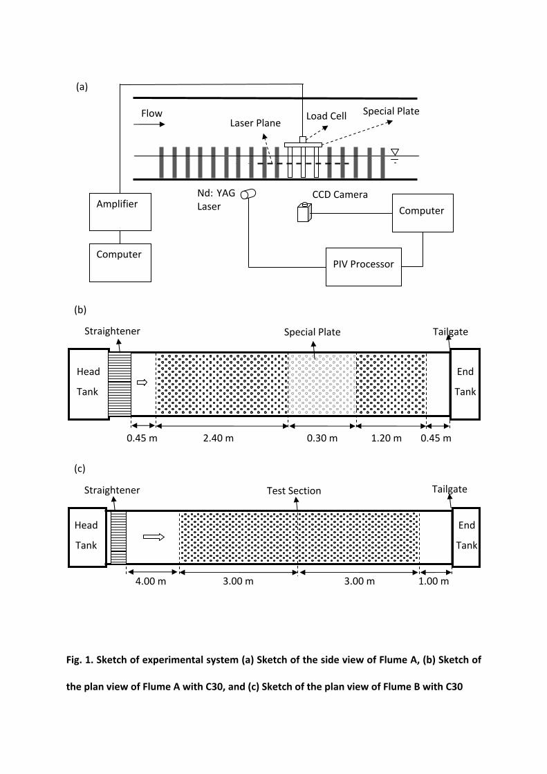
Fig. 1. Sketch of experimental system (a) Sketch of the side view of Flume A, (b) Sketch of

the plan view of Flume A with C30, and (c) Sketch of the plan view of Flume B with C30

Special Plate

Computer

CCD Camera

PIV Processor

Nd: YAG Laser

Flow Load Cell

Amplifier

Computer

Laser Plane

0.45 m

TailgateStraightener

1.20 m 0.30 m0.45 m

Head

Tank

2.40 m

End

Tank

Head

Tank

1.00 m 3.00 m4.00 m 3.00 m

End

Tank

TailgateStraightener

(a)

(b)

(c)

Test Section

Special Plate

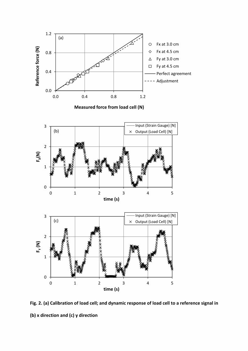
Fig. 2. (a) Calibration of load cell; and dynamic response of load cell to a reference signal in

(b) x direction and (c) y direction

0.0

0.4

0.8

1.2

0.0 0.4 0.8 1.2

Reference force (N)

Measured force from load cell (N)

Fx at 3.0 cm

Fx at 4.5 cm

Fy at 3.0 cm

Fy at 4.5 cm

Perfect agreement

Adjustment

0

1

2

3

0 1 2 3 4 5

F X(N)

time (s)

Input (Strain Gauge) [N]

Output (Load Cell) [N](b)

0

1

2

3

0 1 2 3 4 5

F Y(N)

time (s)

Input (Strain Gauge) [N]

Output (Load Cell) [N](c)

(a)

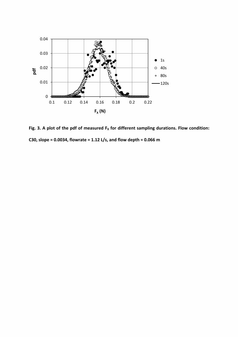
Fig. 3. A plot of the pdf of measured FX for different sampling durations. Flow condition:

C30, slope = 0.0034, flowrate = 1.12 L/s, and flow depth = 0.066 m

0

0.01

0.02

0.03

0.04

0.1 0.12 0.14 0.16 0.18 0.2 0.22

pdf

FX (N)

1s

40s

80s

120s

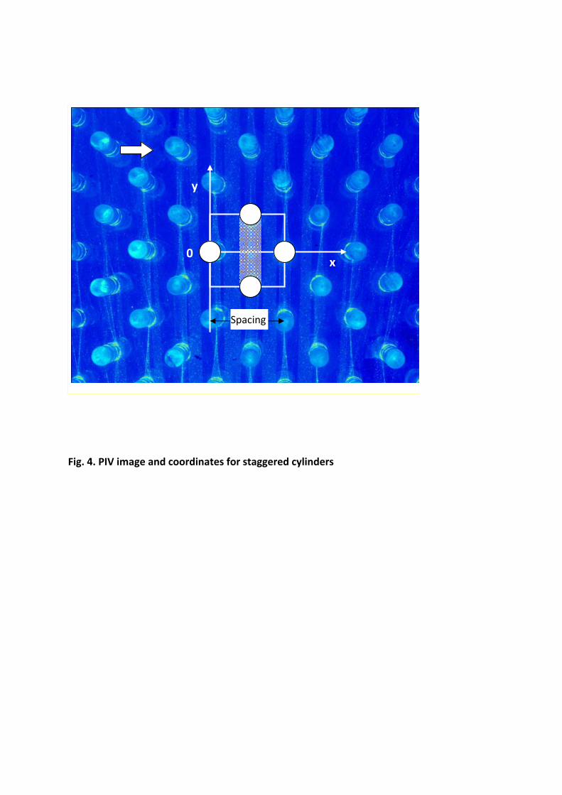
Fig. 4. PIV image and coordinates for staggered cylinders

x

y

0

Spacing

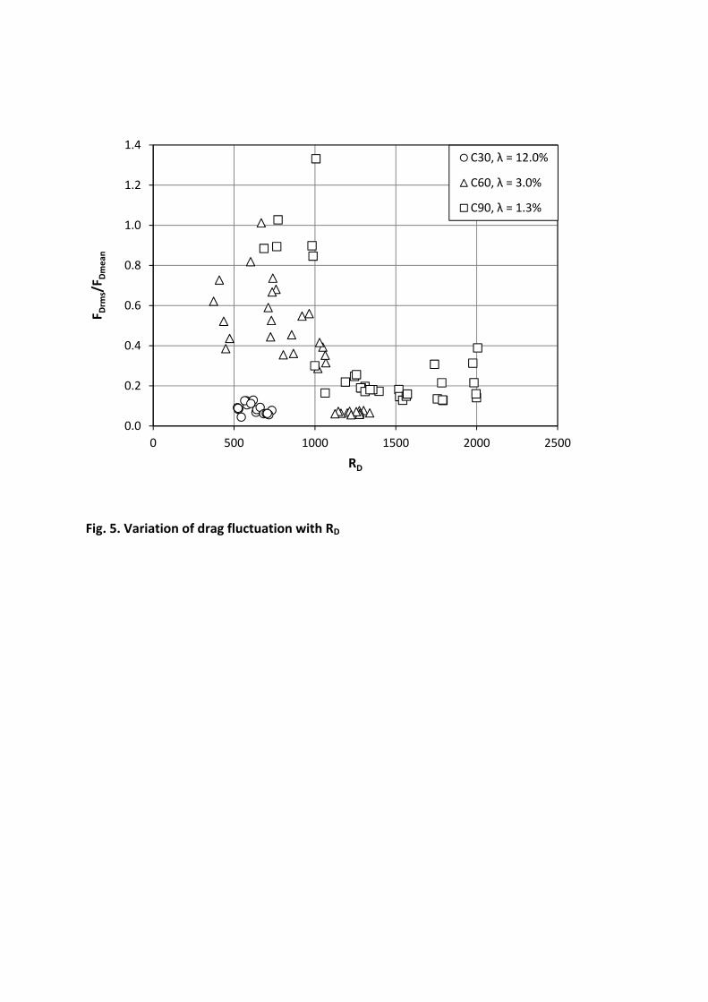
Fig. 5. Variation of drag fluctuation with RD

0.0

0.2

0.4

0.6

0.8

1.0

1.2

1.4

0 500 1000 1500 2000 2500

F Drm

s/F D

mean

RD

C30, λ = 12.0%

C60, λ = 3.0%

C90, λ = 1.3%

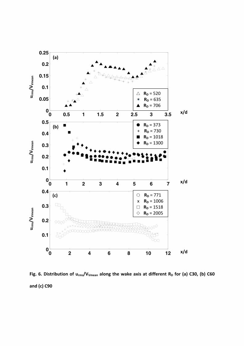
Fig. 6. Distribution of urms/VVmean along the wake axis at different RD for (a) C30, (b) C60

and (c) C90

0 2 4 6 8 10 120

0.1

0.2

0.3

0.4

0 1 2 3 4 5 6 70

0.1

0.2

0.3

0.4

0.5

0 0.5 1 1.5 2 2.5 3 3.50

0.05

0.1

0.15

0.2

0.25

△ RD = 520 ✶ RD = 635 ▲ RD = 706

● RD = 373 + RD = 730 ■ RD = 1018 ◆ RD = 1300

○ RD = 771 x RD = 1006 □ RD = 1518 ◇ RD = 2005

(a)

(b)

(c)

x/d

u rms/VVmean

u rms/VVmean

u rms/VVmean

x/d

x/d

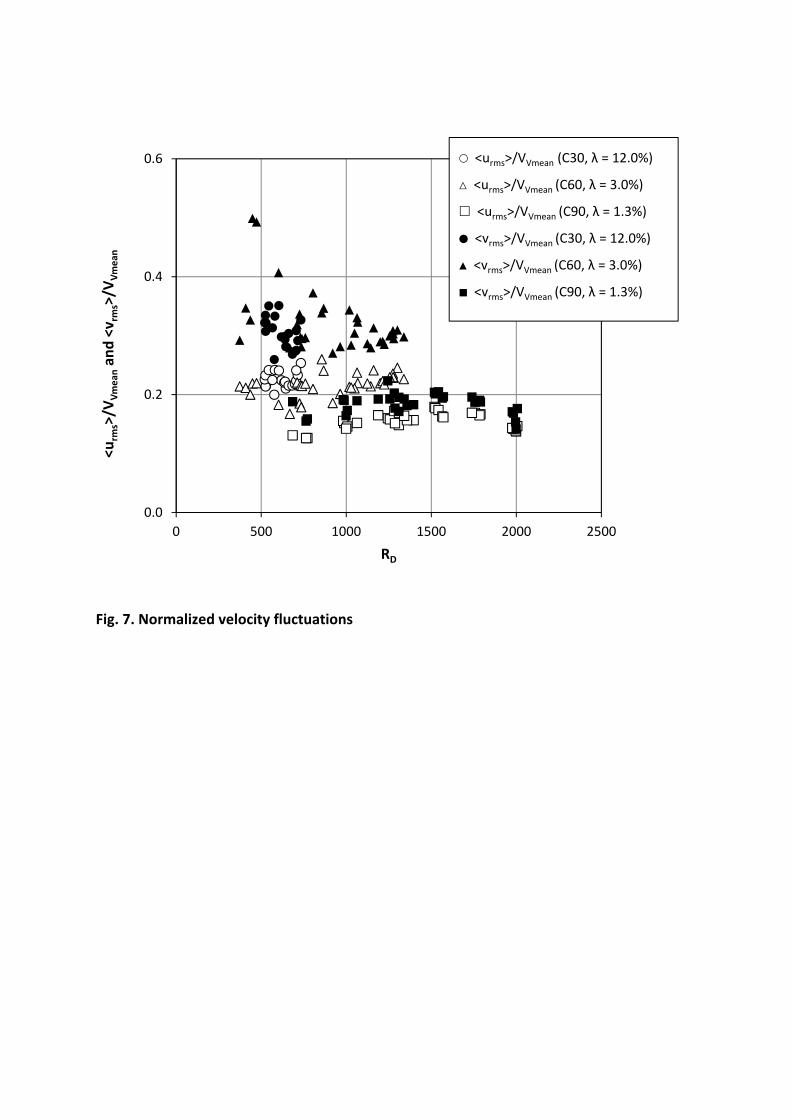
Fig. 7. Normalized velocity fluctuations

0.0

0.2

0.4

0.6

0 500 1000 1500 2000 2500

<urm

s>/V

Vmeanan

d <v

rms>/V

Vmean

RD

ç <urms>/VVmean (C30, λ = 12.0%)

ó <urms>/VVmean (C60, λ = 3.0%)

<urms>/VVmean (C90, λ = 1.3%)

æ <vrms>/VVmean (C30, λ = 12.0%)

ò <vrms>/VVmean (C60, λ = 3.0%)

à <vrms>/VVmean (C90, λ = 1.3%)

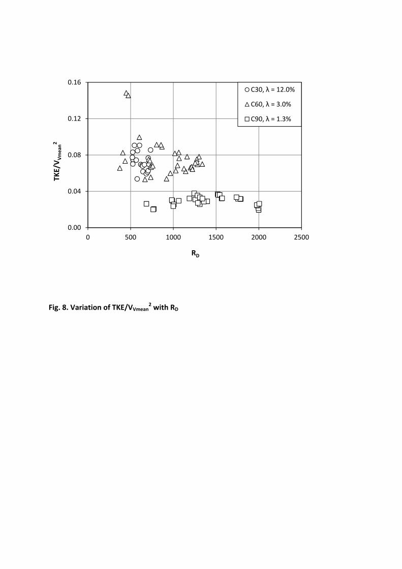
Fig. 8. Variation of TKE/VVmean2 with RD

0.00

0.04

0.08

0.12

0.16

0 500 1000 1500 2000 2500

TKE/VVm

ean2

RD

C30, λ = 12.0%

C60, λ = 3.0%

C90, λ = 1.3%

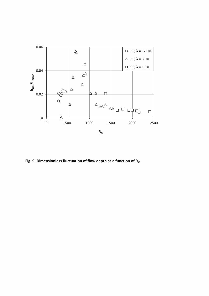
Fig. 9. Dimensionless fluctuation of flow depth as a function of RD

0

0.02

0.04

0.06

0 500 1000 1500 2000 2500

h rms/h m

ean

RD

C30, λ = 12.0%

C60, λ = 3.0%

C90, λ = 1.3%

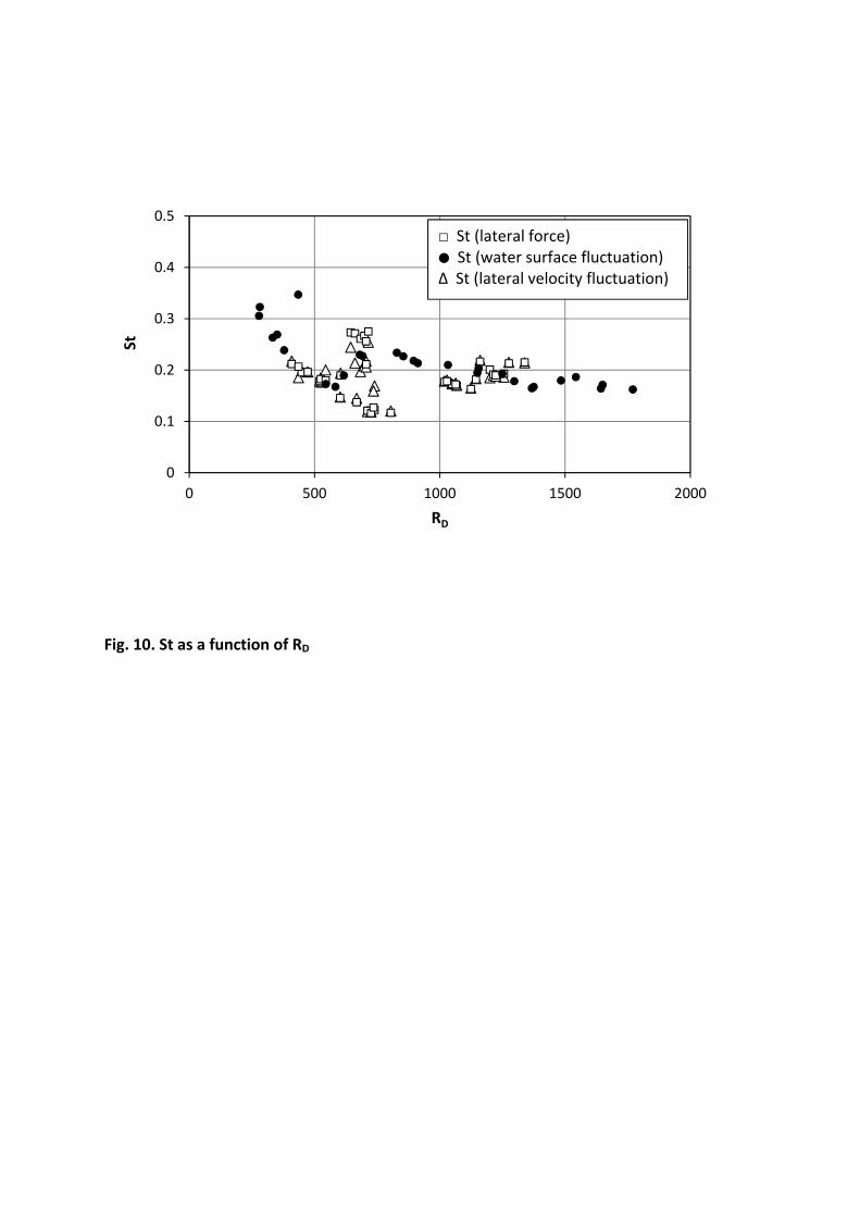
Fig. 10. St as a function of RD

0

0.1

0.2

0.3

0.4

0.5

0 500 1000 1500 2000

St

RD

□ St (lateral force)æ St (water surface fluctuation)∆ St (lateral velocity fluctuation)

Measurements of fluctuation in drag acting on rigid cylinder array in open channel flow

Documents