Measurement of local heat transfer coefficient during gasâ ...

International Journal of Heat and Fluid Flow 45 (2014) 41–52

Contents lists available at ScienceDirect

International Journal of Heat and Fluid Flow

journal homepage: www.elsevier .com/ locate/ i jhf f

Measurement of local heat transfer coefficient during gas–liquid Taylorbubble train flow by infra-red thermography

0142-727X/$ - see front matter � 2013 Elsevier Inc. All rights reserved.http://dx.doi.org/10.1016/j.ijheatfluidflow.2013.12.001

⇑ Corresponding author. Tel.: +91 512 259 7038; fax: +91 512 259 7408.E-mail address: [email protected] (S. Khandekar).

Balkrishna Mehta, Sameer Khandekar ⇑Department of Mechanical Engineering, Indian Institute of Technology Kanpur, Kanpur, UP 208016, India

a r t i c l e i n f o

Article history:Received 12 January 2013Received in revised form 6 October 2013Accepted 2 December 2013Available online 25 December 2013

Keywords:Taylor bubble flowLocal Nusselt numberInfraRed ThermographyDesign of experimentHeat transfer enhancement

a b s t r a c t

In mini/micro confined internal flow systems, Taylor bubble train flow takes place within specific range ofrespective volume flow ratios, wherein the liquid slugs get separated by elongated Taylor bubbles, result-ing in an intermittent flow situation. This unique flow characteristic requires understanding of transportphenomena on global, as well as on local spatio-temporal scales. In this context, an experimental designmethodology and its validation are presented in this work, with an aim of measuring the local heat trans-fer coefficient by employing high-resolution InfraRed Thermography. The effect of conjugate heat transferon the true estimate of local transport coefficients, and subsequent data reduction technique, is dis-cerned. Local heat transfer coefficient for (i) hydrodynamically fully developed and thermally developingsingle-phase flow in three-side heated channel and, (ii) non-boiling, air–water Taylor bubble train flow ismeasured and compared in a mini-channel of square cross-section (5 mm � 5 mm; Dh = 5 mm, Bo � 3.4)machined on a stainless steel substrate (300 mm � 25 mm � 11 mm). The design of the setup ensuresnear uniform heat flux condition at the solid–fluid interface; the conjugate effects arising from the axialback conduction in the substrate are thus minimized. For benchmarking, the data from single-phase flowis also compared with three-dimensional computational simulations. Depending on the employed vol-ume flow ratio, it is concluded that enhancement of nearly 1.2–2.0 times in time-averaged local stream-wise Nusselt number can be obtained by Taylor bubble train flow, as compared to fully developed single-phase flow. This enhancement is attributed to the intermittent intrusion of Taylor bubbles in the liquidflow which drastically changes the local fluid temperature profiles. It is important to maintain properboundary conditions during the experiment while estimating local heat transfer coefficient, especiallyin mini-micro systems.

� 2013 Elsevier Inc. All rights reserved.

1. Introduction

Transport mechanisms of heat, momentum and species undertwo-phase flow conditions in mini/micro systems are greatly af-fected by local distribution of the phases or flow patterns in thechannel. Taylor bubble train flow, a sub-set of slug flows occurringin mini/micro-systems, is typically characterized by a sequence oflong bubbles which are trapped in between liquid slugs. Geometri-cal distribution of the liquid slugs and bubbles is fundamentallygoverned by the resultant of gravity, surface tension, inertia andviscous effects. For a given liquid–gas system, interplay betweenthe gravity and surface tension forces mainly depends on the sizeof the channel, i.e. the applicable Bond number (Bo). When surfacetension dominates over gravitational body force, Taylor bubblesadopt the characteristic capsular shape, with a liquid thin film sep-arating the gas/vapor phase with the wall. In horizontal flow con-ditions when Bo is high enough (Bo > Bocr � 1.835 (Bretherton,

1961)), gravity force dominates over surface tension and the liquidfilm essentially takes the lower part of the channel cross-section,whereas in the upper part, a negligibly thin liquid film may ormay not exist. The existence of liquid film on the wall dependson Ca and surface energy characteristics (hydrophobic or hydro-philic) of the channel wall (Serizawa et al., 2002; Cubaud and Ho,2004; Ajaev and Homsy, 2006).

Taylor bubble train flow is expected to occur and, is employedin many new and upcoming systems and devices in diversebranches of engineering ranging from bio-medical, bio-chemicalto thermal management of electronics, micro-two-phase heatexchangers and reactors, nuclear rod bundles, micro-fluidic de-vices, loop heat pipes, etc. (Triplett et al., 1999; Devesenathipathyet al., 2003; Spernjak et al., 2007; Moharana et al., 2011a). Quitefrequently, due to the mini/micro fabrication techniques, such aslaser machining, chemical etching, micro-milling, abrasive jetmachining etc., emerging technological solutions employing inter-nal convective flows, make use of channels of non-circular crosssections. Rectangular micro-channels are of particular interest asthey are used extensively in heat sinks of microelectronic devices,

Nomenclature

A area of cross section (m2)cp specific heat at constant pressure (J/kg K)Dh hydraulic diameter (m)Df number of framesh heat transfer coefficient (W/m2 K)J phase superficial velocity (m/s)k thermal conductivity (W/m K)‘ length specified in image (m)L length of the channel, characteristic length (m)m ratio of relative bubble velocity to bubble velocity (�)N number of observed bubblen frames per secondp perimeter (m)Q volumetric flow rate (m3/s), heat input (W)q00 heat flux (W/m2)R radius (m)S slip ratio (�)T temperature (K)T� non-dimensional temperature (�)t time (s), thickness (m)U velocity (m/s)x gas fraction (�)Z distance from inlet (m)Z� thermal non-dimensional distance (=Z/Re�Pr�Dh)

Greek symbolsd substrate thickness (m)b volume flow ratio (�)e void fraction (�)

g liquid film thickness (m)f frequency of bubbles (Hz)l dynamic viscosity (Pa s)q mass density (kg/m3)u heat flux ratio (�)w ratio of bubble velocity to total superficial velocity (�)r surface tension (N/m)

Non-dimensional numbersBo Bond number Dh � fðql � qgÞ � g=rlg0:5

Ca Capillary number ðll � Ub=rlÞNu Nusselt number ðh � Dh=klÞPr Prandtl number ðll � cp=klÞRe Reynolds number ðql � J � Dh=llÞ

Subscriptsb bubble, bulk, basef fluidg gash hydraulic, hydrodynamicin inputl liquids slugsf solid–fluidtot totalTP two-phaseuc unit cellw wall

42 B. Mehta, S. Khandekar / International Journal of Heat and Fluid Flow 45 (2014) 41–52

as well as for catalytic reactors for micro-fuel processors, biologicalsensors, lab-on-chip devices, water management of PEM fuel cells,high heat flux dissipating heat exchanger equipment etc. Mostly inthese mini/micro-scale devices, heat transfer process is conjugatein nature, i.e. the diffusion in the solid wall of the channel affectsthe thermal boundary condition (uniform heat flux or uniform walltemperature) which the fluid experiences at the solid–fluid inter-face. This conjugate nature of thermal transport increases the levelof complexity in the estimation of local heat transfer, demandingan effective means of accurate non-intrusive field measuringinstruments as against intrusive point measurements, such as bymicro thermocouples (Majumder et al., 2013). In this context Infra-Red Thermography (IRT) has emerged as an effective non-intrusivefield measurement technique in the recent past (Hetsroni et al.,1996, 2003) to address the local measurement of a variety of com-plex problems involving high spatial temperature gradients. In thepresent work, we have made an attempt to estimate the local heattransfer coefficient under such demanding conditions involving (i)Intermittent Taylor bubble train flow, (ii) non-circular (square)mini-channel, by employing non-intrusive field measurement byInfraRed Thermography. The paper presents an experimental de-sign methodology so that local heat transfer can be estimated byminimizing the conjugate heat transfer effects in the system. Aswill be revealed in the survey of open literature, which is presentedin the subsequent section, understanding of local species transportunder such flow conditions is quite an involved problem.1

1 It must be noted here that the issue of accurate experimental measurement of thebulk mean-mixing temperature of the respective fluid-phases, under such intermit-tent flow conditions, is not trivial. The procedure adopted in this work to estimate thistemperature requires further refinement (refer Section 3.3). Other major aspectstowards estimating the correct local heat transport parameters have been included inthe design of the experiment presented here.

2. Literature review

In one of the seminal works on Taylor bubble flows, it was ob-served that a bubble does not rise spontaneously in a water filledvertically oriented circular capillary under the effect of gravityfor Bo < 1.835 (Bretherton, 1961) and film thickness scaling wasfound as (g/R) � Ca2/3, valid for 10�3

6 Ca 6 10�2. Deposition ofthin liquid film due to displacement of the wetting fluid by a gasbubble inside a circular capillary wall has been studied (Fairbroth-er and Stubbs, 1935) and another scaling for film thickness was gi-ven as (g/R) � Ca1/2 for 10�5

6 Ca 6 10�1. Under Taylor bubbletrain flow conditions, the bubble velocity will not be equal to theliquid due to the existence of liquid film that separates the bubblefrom the wall (Fabre and Line, 1992; Thulasidas et al., 1995, 1997).Presence of bubble interfaces at front and back of the liquid slugsmodifies the flow field inside it. Circulation takes place inside theliquid slug due to existing wall shear stress, which in turn en-hances the species transport. It has been hypothesized that forlow Ca, circulation patterns in the liquid slug will be observed withpaired set of vortices, which tend to disappear for higher Ca, lead-ing to bypass flows (Taylor, 1961). More recent numerical andexperimental studies (Taha and Cui, 2004, 2006; Kashid et al.,2005; He et al., 2010; Bajpai and Khandekar, 2012) have confirmedthese findings. In recent years focus on Taylor bubble flows in non-circular channels has also attracted attention. Shape of the bubblecross-section in a square capillary has been experimentally deter-mined and it is concluded that for Ca 6 0.1, bubble cross-section isnon-axisymmetric. As the total superficial velocity increases andCa becomes greater than 0.1, the increased inertia forces tend tomake the bubble cross-section axisymmetric (Kolb and Cerro,1993; Han and Shikazono, 2009). Numerical study of the flow oflong bubble in a square capillary suggested that liquid depositionon capillary wall is a function of flow Ca (Kamisli, 2003). Flow pat-

B. Mehta, S. Khandekar / International Journal of Heat and Fluid Flow 45 (2014) 41–52 43

tern transition and frictional pressure drop has been investigatedin different rectangular channels, and correlations to predict them,including the Chisholm’s factor (estimates the slip ratio S, based onannular flow model, defined as: S ¼

ffiffiffiffiffiffiffiffiffiffiffiffiffiffiffiffiffiffiffiffiffiffiffiffiffiffiffiffiffiffiffiffiffiffiffiffi1� xð1� ql=qgÞ

q, where x is

quality of gas-phase), have been reported (Ide and Matsumura,1990; Mishima et al., 1993; Chen et al., 2009).

Study of heat transfer in gas–liquid two-phase flow revealedhigher heat transfer coefficient than equivalent single-phaseflows. Very small temperature gradient exists beneath the bub-ble which enhances the heat transfer whereas in the liquid slugs,existence of circulating flow due to presence of bubble interfacesat front and back enhances local heat transfer (Bao et al., 2000;Fukagata et al., 2007; Narayanan and Lakehal, 2008; Gupta et al.,2010). Experimental investigation of heat transfer in non-boilingtwo-phase slug flow in a circular channel of diameter 1.5 mmusing InfraRed Thermography (IRT) has been reported by Walshet al. (2010). Similar study using micro-thermometry in non-cir-cular (square) mini-channel of Dh = 3.3 mm has been recentlydone by Majumder et al. (2013). Both studies reveal that suchflows can be highly efficient in enhancement of heat transfer,as compared to fully developed single-phase flows. Severalnumerical studies of Taylor slug flow have also been reportedin recent times which highlighted the effect of L/D, Pr, Ca, onthe heat transfer and shear stress (Asadolahi et al., 2011; Bajpaiand Khandekar, 2012). Detailed computational simulations,including the thin film surrounding the gas bubble, have beenreported using the VOF method and an overall enhancementup to 610% in the heat transfer has been reported (Mehdizadehet al., 2011). Simulation of a ‘unit-cell’ using periodic boundarycondition with moving frame of reference revealed the limita-tions of assuming 2-D axisymmetric conditions; in reality theflow becomes three-dimensional in nature, especially forReTP P 950 (Asadolahi et al., 2012; Talimi et al., 2012a). Recentmicro-PIV studies on circular and non-circular channels clearlyreveal the flow recirculations inside the liquid slugs and theeffect of gravity on film thickness and heat transfer (Leunget al., 2012; Zaloha et al., 2012). In a recent extensive review,Talimi et al. (2012b) emphasized that, looking into the designneed of several upcoming engineering systems and technologies,extensive exploration of hydrodynamics and heat transfer ofTaylor slug flow in the non-circular ducts, under differentthermal boundary conditions must be undertaken.

As has been pointed out earlier, convective flows in mini/microgeometries are prone to the effects of conjugate heat transfer con-ditions within the solid substrate in which the flow takes place,affecting the overall heat transfer performance (Nonino et al.,2009; Moharana et al., 2011b). Maranzana et al. (2004) proposeda new criterion for quantifying the effect of axial conduction inmini/micro systems. Simultaneously developing single-phase lam-inar flow in rectangular mini-channel array was studied and it wasconcluded that axial conduction in the substrate becomes signifi-cant for higher values of Axial Conduction Number i.e., M P 0.01.

M ¼ q00cond

q00conv¼ kw

W � p=Lqf � Cpf � df � p � u

!ð1Þ

Here, q00cond gives the first-order estimation of the axial heat fluxin the wall, assuming the heat transfer is one dimensional alongthe length of the channel through the same temperature differencewhich the fluid experiences between channel inlet and outlet. Theparameter M allows the comparison of the axial heat transfer byback conduction in the substrate wall to the convective heat trans-fer (q00conv) to the fluid. Naturally, if the value of M is high, axial con-duction effects are important and cannot be neglected. Eq. (1) canbe rewritten as:

M ¼ 1ðRe � PrÞ

Dh

L

� �� W

df

� �� kw

kf

� �ð2Þ

Lee et al. (2005) and Lee and Garimella (2006) conducted a 3-Dconjugate laminar heat transfer analysis, including entrance ef-fects, for single channels as well as micro-channel heat sinks, sub-jected to uniform heat flux imposed on the bottom of the substrate.Operating regimes and boundary conditions wherein conjugate ef-fects become important were identified. Correlations to predict lo-cal and average Nusselt number were also proposed.

Conjugate effects during convective flows also pose challengefor designing of experimental setup for proper measurement ofheat transfer coefficient. In addition, data reduction process hasto be carefully addressed so that errors in estimation due to theconjugate effects do not arise. In general, the local Nusselt numbergets affected by the distortion of the thermal boundary conditiondue to axial back conduction in the substrate/pipe/channel wall.The geometrical parameters of the channel, flow Reynolds number,the area ratio (Asf) and the thermal conductivity ratio (ksf) havebeen recognized as the primary influencing parameters in the anal-ysis of conjugate heat transfer (Celata et al., 2006; Nonino et al.,2009; Rao and Khandekar, 2009; Moharana et al., 2012). In thiscontext, point measurement systems such as thermocouples haveobvious limitations to quantify the extent of the conjugate effectson thermal transport behavior. In such a situation therefore, com-plete field information is necessary to estimate the spatial temper-ature gradients in the wall and fluid region, a recent example ofwhich is the use of InfraRed Thermography (IRT) for estimatinglocal heat transfer coefficient during single-phase thermally devel-oping flows with conjugate effects (Mehta and Khandekar, 2012).

In recent past, IRT has sufficiently evolved as a versatile tech-nique for the measurement of heat transfer in single-phase flows,two-phase flows in micro-scale systems, high enthalpy flows, mul-ti-jet systems, jet impingements on rotating disks, jet in cross flow,space radiator plates etc. (Hetsroni et al., 1996, 2003; Astarita et al.,2000; Hemadri et al., 2011). The limitations of the technique,including the sources of measurement errors, calibration issues,emissivity corrections, effect of participating media, noise isola-tion, data reduction issues have also been addressed (Sargentet al., 1998; Buchlin, 2010; Hetsroni et al., 2011).

Literature review clearly suggests that: (i) Limited studies areavailable on experimental investigation of heat transfer in Taylorbubble train flows in non-circular mini/micro channels. (ii) Localtransport parameters are not usually addressed; at present, suchinformation is only available in numerical simulations, most ofwhich focus on circular channels. In addition, most experimentalstudies rely on point measurements. (iii) Very few studies addressconjugate effects and non-standard boundary conditions in Taylorbubble train flow situations, which frequently arise in mini/microsystems. In such situations the design of experiment becomescritical.

In this work estimation of local heat transfer coefficient for Tay-lor bubble train flow in a square mini-channel of size5 mm � 5 mm by non-intrusive InfraRed Thermography has beenundertaken. The experimental setup design must ensure that con-jugate nature of heat transfer does not adversely affect the trueestimation of heat transfer coefficient for Taylor bubble train flow.The design of the experiment is addressed next.

3. Design of experiment

Before attempting to measure local heat transfer coefficient un-der Taylor bubble train flow situation, the experimental designmust be benchmarked against single-phase flow. Most of theanalytical solutions for fully-developed or developing convective

44 B. Mehta, S. Khandekar / International Journal of Heat and Fluid Flow 45 (2014) 41–52

single-phase flows are available for standard boundary conditionswith no conjugate effects (Shah and London, 1978). In situationswhere non-standard boundary conditions are applicable and/orconjugate effects are encountered, problem of estimating the heattransfer coefficient has to be either tackled through computationaltechniques and/or through an experimental route. If accurate heattransfer coefficient needs to be experimentally determined in a gi-ven non-standard system, the protocol must be such that conju-gate effects are either (i) completely isolated or quantifiable (ii)minimized so as to ascertain the true local heat transfer coefficient.

The design procedure for the experimental setup involves sev-eral steps. Firstly, viscous dissipation in the liquid can be neglectedfor the range of parameters considered in this study. Secondly,while the Peclet number considered in this work are large enoughto assume that the axial conduction in the fluid domain will benegligible, only the axial back conduction in the solid substratemust be minimized and quantified. Under single-phase flow condi-tions, guidelines for minimizing and quantifying the conjugate ef-fects due to the solid substrate are available in the literature(Maranzana et al., 2004; Nonino et al., 2009; Moharana et al.,2011b). As discussed earlier, guidelines provided by the axial con-duction number M provides the first-order working guideline fordesigning systems with minimal effects of axial back conductionin solid substrates. A low value of M is desirable, which ensuresthat axial conduction in the substrate will not affect the natureof boundary condition experienced by the fluid at the fluid–solidinterface. This has been achieved in the present setup by employ-ing computational simulation of heat and fluid flow through itera-tive design procedure, the nuances of which will be described inSection 3.2. The final geometrical parameters of the experimentalsetup, as described next, evolved as a result of the computationaldesign simulations.

3.1. Description of the experimental setup

Schematic details of the experimental setup are shown inFig. 1(a–d). The heated test section consists of a single squaremini-channel with cross section area = 5 mm � 5 mm,

Fig. 1. Schematic details of the

Dh = 5.0 mm, machined on a stainless steel substrate (k = 16 W/m K; ksf = 25; M = 0.0014), dimensions of which are300 mm � 25 mm � 11 mm. The basis of these dimensions willbe scrutinized in Section 3.2. In the upstream direction of theheated section, there is a 300 mm visually transparent unheatedchannel length of polycarbonate material which is provided forthe complete hydrodynamic flow development in the entire rangeof Re applicable to the single-phase flow experiments. Two-phaseTaylor bubble train flow (degassed and deionized water asliquid-phase and dry air as gaseous-phase) is generated with thehelp of an air injection system (T-junction) located far upstream.In the present case, both the connectors/arms constituting theT-junction have exactly the same cross-section, i.e., square sectionof size 5 mm � 5 mm. Constant temperature bath (Make: Julabo�

F34 ME, precision ± 0.1 K) is used to supply the water and dry-airis supplied from a pressurized cylinder through the T-junction(Fig. 1). In the case of Taylor bubble train flow, the unheated lengthprovides necessary flow stabilization after air bubbles get formedat the T-junction. In addition, it is also used to visualize the Taylorbubbles before they enter the heated test section. This visualiza-tion has been done by using Photron-Fastcam�-SA3 high speedcamera. Image acquisition has been done at 500 fps for all the Tay-lor bubble train flow experiments. It must be noted here that thedesign of the T-junction (which includes diameter ratio of liquidsupply arm to that of the gas supply arm, internal edge geometry,wettability of the material, etc.) determines the resulting bubblepatterns formed by it.

Fluid temperature at inlet (Tfi), outlet (Tfo) and at three otherlocations (Tf1-Tf3) in the heated test section have been measuredby suitably located K-type micro thermocouples (Omega�,0.13 mm bead diameter, precision ± 0.1 after calibration), as shownin Fig. 1(a) and (c). The time constant of these thermocouples are ofthe order of 10�4 s, which ensured sufficient dynamic response. Inaddition to these five thermocouples for fluid temperature mea-surement, three more K-type pre-calibrated thermocouples Tw1-Tw3 are embedded in the wall of the heated test section, as detailedin Fig. 1(a) and (c). All thermocouple data acquisition has been car-ried out at 30 Hz by using a high precision 24 bit PCI-DAQ card

experimental test setup.

B. Mehta, S. Khandekar / International Journal of Heat and Fluid Flow 45 (2014) 41–52 45

(Make: National Instruments�, NI 9213). All thermocouples arecalibrated against standard Pt-100 NIST traceable thermocouple.

The cylindrical DC supplied cartridge heater is located awayfrom the actual fluid–solid interface, as shown. Precise digital mul-ti-meter (precision ± 0.1 V and ± 0.01 A) is used to measure theelectrical power dissipation of the heater. Necessary insulation isprovided to the entire setup by plexi-glass/foam blocks, includingthe top of the channel, as shown. Apart from the standard energybalance technique, heat losses were also estimated by conductingthe experiments in the no flow condition for different heat inputs,respectively, and recording the steady-state IR thermogram andwall thermocouple temperature. In such a condition, whateverheat was supplied to the system got dissipated to the environment.Therefore, different values of average surface temperature corre-sponding to the different heat inputs have been obtained and usedfor estimating heat lost during the actual experiments. With boththese complementary methodologies, it was found that the maxi-mum losses never exceeded 8% - 11% of the gross input.

The IR camera used (Make: FLIR�, Model: SC4000; IndiumAntimonide detector array) has an operational spectral band of3–5 lm, 14 bit signal digitization and a Noise Equivalent TemperatureDifference of less than 0.02 K at 30 �C. As shown in Fig. 1, thespatial temperature field of the front side of the substrate havingan area 25 mm � 290 mm is captured by the IR camera. A very thinuniform spray coating of high emissivity black paint (Make:Nextel� e > 0.95) has been done on this side to ensure reliable IRmeasurements. Apart from this, the experiment has been set-upin a dark room with non-reflecting background to minimize thesurrounding radiation. As the maximum Biot number in theX-direction based on the channel wall thickness, t (Bi = ht/kw), isof the order of 0.09 (< 0.1), lumped assumption will hold and tem-perature gradient in that direction will be negligible. The recordingof spatial IR thermographic profiles of the front surface of the sub-strate is facilitated by a 5 mm thick InfraRed transmitting CaF2

glass window (Make: Crystran�; Transmissivity: 95%, for wave-length 2 lm - 7 lm; Refractive index = 1.399 at 5 lm; k = 9.71Wm�1K�1). IR images have also been acquired at 30 Hz and postprocessed by using ThermaCAMTM Researcher-V2.9 software. IRthermograms are captured at 320 pixels � 256 pixels which givea spatial resolution of 900 microns in the Z-direction and 750 mi-crons in the Y-direction. While the software incorporates protocolsfor corrections due to ambient temperature, ambient humidity andabsorptivity of the medium, local emissivity of the target must besupplied by conducting in situ calibration against standard tem-perature measurement technique. Before conducting the experi-ments, the text assembly (including the CaF2 glass window) wascalibrated in the entire range of operating temperatures by simul-taneous measure of surface temperature by a NIST traceable Pt-100thermocouple and IR camera. The emissivity matrix thus generatedwas supplied to the software for post processing to get the correcttemperature field. In addition, during the experiments, as has beendescribed earlier, four thermocouples were always kept for refer-encing. Several independent benchmarking and validation experi-ments for precise calibration of the camera were also conducted,as detailed in Mehta and Khandekar (2012).

3.2. Computational design procedure

To evolve the design of the above experimental setup and toundertake benchmarking of the data, 3-D computational simula-tions of single-phase laminar flow were first carried out onANSYS�-Fluent, on two separate geometries, as detailed inFig. 1(d). In Simulation #1, fluid flow and heat transfer is studiedin a square channel, uniformly heated from three sides while thetop side is kept insulated, i.e., no conjugate effects are taken; thegoverning equations for fluid flow and heat transfer are only solved

in the fluid domain. Thus, Simulation #1 serves as a benchmark forthe non-conjugate situation. Simulation #2, on the other hand, de-picts the current experimental situation wherein the conjugateheat transfer problem is solved taking the heat flow through thesolid substrate domain also. Here, heat flux is applied at the bot-tom of the solid substrate (representing the heater, as done inthe experiment), which is located away from the solid–fluidboundary, while all other side walls were kept insulated, as shown.The geometrical, thermophysical and flow parameters, for exam-ple, the length L, the width W, the thermal conductivity of the sub-strate kw, and flow Re were varied to obtain different range of theaxial conduction parameter M, on the conjugate physical domain,as depicted in Fig. 1(a) and (b). Flow conditions in both the simu-lations are kept hydrodynamically fully developed and thermallydeveloping i.e., Graetz type flow, exactly as per the experimentalconditions. Both simulated geometries correspond to channelcross-section = 5 mm � 5 mm and inlet Prandtl number is keptconstant = 5.0, corresponding to water. Computational domainsdepicting these geometries were created using hexahedral gridsystem on Gambit� 2.3. The flow Re was changed so that the axiallength L of the channel will cover the entire range from thermallydeveloping to thermally fully developed conditions at the exit. Thecomplete problem formulation, including the details of the conser-vation equation for mass, momentum and energy, as applicable toboth the cases, numerical schemes to solve the governing equa-tions and grid independence has been discussed in detail in Mehtaand Khandekar (2012), and therefore, not repeated here for brevity.

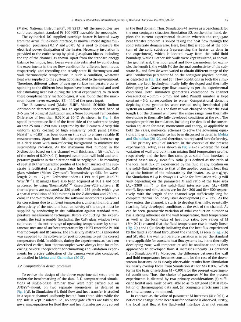
The primary result of interest, in the context of the presentexperimental setup, is as shown in Fig. 2(a–d), wherein the axialvariation of wall and bulk mean mixing fluid temperature profile,respectively, and the heat flux ratio, u, at solid–fluid interface isplotted based on Ab. Heat flux ratio u is defined as the ratio ofthe local heat flux q00z , experienced by the fluid at any location onthe solid–fluid interface to that of the applied constant heat fluxq00 at the bottom of the substrate by the heater, i.e., u ¼ q00z=q00.For Simulation #1 u is always = 1 while for Simulation #2, u willvary depending on the parameter M and ratio of the base area(Ab = 3300 mm2) to the solid–fluid interface area (Asf = 4500mm2). Reported simulations are for Re = 200 and Re = 500 respec-tively, with the length of the channel kept sufficiently long forcomplete thermal boundary layer development (Z⁄ = 0.25). As theflow enters the channel, it starts to develop thermally, eventuallyreaching fully developed conditions at the exit of the channel. Ascan be seen, parametric variation of axial conduction number Mhas a strong influence on the wall temperature, fluid temperatureas well as the local value of heat flux ratio. Low values of M(M < 0.01) ensured that the fluid temperature rise is nearly linear(Fig. 2(a) and (c)); clearly indicating that the heat flux experiencedby the fluid is constant throughout the channel, as seen in Fig. 2(b)and (d). Also, the wall temperature variation is as per the standardtrend applicable for constant heat flux systems i.e., in the thermallydeveloping zone, wall temperature will be nonlinear and as flowapproaches to developed flow, it increases linearly (as obtainedfrom Simulation #1). Moreover, the difference between the walland fluid temperature becomes constant for the rest of the down-stream locations. As is clearly observable, results from Simulation#2 nearly overlap those from Simulation #1 for M < 0.002, whichforms the basis of selecting M = 0.0014 for the present experimen-tal conditions. Thus, the choice of parameter M for the presentexperiments is dictated by two primary considerations (i) suffi-cient frontal area must be available so as to get good spatial reso-lution of thermographic data and, (ii) conjugate effects must alsobe simultaneously minimized.

In contrast, as the value of parameter M increases (M > 0.01), anoticeable change in the heat transfer behavior is observed. Firstly,the local heat flux at the fluid–solid interface does not remain

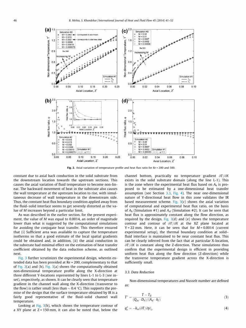
Fig. 2. Axial variation of temperature profile and heat flux ratio for Re = 200 and 500.

46 B. Mehta, S. Khandekar / International Journal of Heat and Fluid Flow 45 (2014) 41–52

constant due to axial back conduction in the solid substrate fromthe downstream location towards the upstream sections. Thiscauses the axial variation of fluid temperature to become non-lin-ear. The backward movement of heat in the substrate also causesthe wall temperature at the upstream location to rise, with simul-taneous decrease of wall temperature in the downstream side.Thus, the constant heat flux boundary condition applied away fromthe fluid–solid interface seems to get severely distorted as the va-lue of M increases beyond a particular limit.

As was described in the earlier section, for the present experi-ment, the value of M was equal to 0.0014, an order of magnitudelower than what is suggested by the computational simulationsfor avoiding the conjugate heat transfer. This therefore ensuredthat (i) Sufficient area was available to capture the temperatureisotherms so that a good estimate of the local spatial gradientscould be obtained and, in addition, (ii) the axial conduction inthe substrate had minimal effect on the estimation of heat transfercoefficient obtained by the data reduction scheme, as outlinednext.

Fig. 3 further scrutinizes the experimental design, wherein ex-tended data has been provided at Re = 200, complementary to thatof Fig. 2(a) and (b). Fig. 3(a) shows the computationally obtainednon-dimensional temperature profile along the X-direction atthree different Y-locations represented by lines L-1 to L-3 (see in-set), respectively, as shown. It can be clearly seen that temperaturegradient in the channel wall along the X-direction (transverse tothe flow) is rather small (less than � 0.4 �C). This supports the pre-mise of the design that the surface temperature obtained by IR is afairly good representative of the fluid–solid channel walltemperature.

Looking at Fig. 3(b), which shows the temperature contour ofa XY plane at Z = 150 mm, it can also be noted that, below the

channel bottom, practically no temperature gradient @T=@Xexists in the solid substrate domain (along the line L-1). Thisis the zone where the experimental heat flux based on Ab is pro-posed to be estimated by a one-dimensional heat transferassumption (see Section 3.3, Fig. 4). The near one-dimensionalnature of Y-directional heat flow in this zone validates the IRbased measurement scheme. Fig. 3(c) shows the axial variationof computational and experimental heat flux ratio, on the basisof Ab (Simulation #1) and Asf (Simulation #2). It can be seen thatheat flux is approximately constant along the flow direction, asrequired by the design. Fig. 3(d) and (e) shows the temperaturecontour and contour of @T=@X at the XZ plane located atY = 22 mm. Here, it can be seen that for M = 0.0014 (currentexperimental setup), the thermal boundary condition at solid–fluid interface is maintained to be near constant heat flux. Thiscan be clearly inferred from the fact that at particular X-location,@T=@X is constant along the Z-direction. These simulations thusconfirm that the experimental design is efficient in providinguniform heat flux along the flow direction (Z-direction) whilethe transverse temperature gradient across the X-direction issufficiently small.

3.3. Data Reduction

Non-dimensional temperatures and Nusselt number are definedas:

T� ¼ T � Tfi

ðQ in � DhÞ=ðAsf � kf Þð3Þ

q00z ¼ �kwð@T=@yÞz ð4Þ

Fig. 3. (a) Wall Temperature variation across the thickness (X-direction) for Re = 200. (b) Temperature contour of central plane (Z = 150 mm) across the thickness for Re = 200.(c) Axial variation of heat flux ratio estimated for heated area for Re = 200. (d) Temperature contour of plane (Y = 22 mm) along the Z-direction for Re = 200. (e) Contour ofoT/oX along Z-direction for Re = 200.

B. Mehta, S. Khandekar / International Journal of Heat and Fluid Flow 45 (2014) 41–52 47

Nuz ¼q00z � Dh

ð�Tw � �Tf Þ � kfð5Þ

Local heat flux q00z is calculated from experimentally obtained IRthermograms, as explained in Fig. 4.

3.3.1. For experimental data reduction�Tw = local wall temperature at any given location along the Z-

axis, averaged along the direction of Y-axis, over the front face ofthe channel wall, as shown in Fig. 4.

It will be appreciated that there is no straight-forward experi-mental way to determine the bulk mean mixing temperature ofthe fluid �Tf . From an experimental point of view there are two pos-sibilities, either to use:

(a) �Tf ¼ �Tf�th = local fluid temperature measured at point byembedding a thermocouple in the channel cross sectionalong the streamwise direction. In the present experimentthis has been done by placing five thermocouples, locatedas shown in Fig. 1(c). However, this is not the true represen-tation of the bulk mean mixing temperature of the fluid.

or

(b) �Tf ¼ �Tb = local bulk mean mixing fluid temperature based onheat balance, assuming that constant heat flux is maintainedthroughout the length of the channel, at the fluid–solidinterface. This is adopted by most researchers, in theabsence of any other means of estimation.

Fig. 4. Schematic explaining the estimation of local heat flux using 1-D conduction approximation from IR thermogram (Mehta and Khandekar, 2012).

48 B. Mehta, S. Khandekar / International Journal of Heat and Fluid Flow 45 (2014) 41–52

For the present experiments too, both the methodologies havebeen adopted for data reduction and comparison. For each experi-mental run, time-averaged wall and fluid temperatures, �Tw and�Tf ð¼ �Tf�thÞ, respectively, are numerical estimated from the localthermocouple data integrated over 60 s (at 30 Hz we get 1800 datapoints), after quasi-steady state is achieved. In addition, eachexperimental run also provides an estimate of bulk mean mixingtemperature �Tf ¼ �Tb. As will be demonstrated and discussed later,this latter approach can lead to serious errors in the estimation ofNusselt Number, especially when conjugate effects are predomi-nant and/or parameter M is large.

3.3.2. For numerical data reduction�Tw = local peripheral averaged heated wall temperature, at the

fluid–solid interface, at any given location along the Z-axis.�Tf ¼ �Tb = local bulk mean mixing fluid temperature at the fluid

cross-section of interest along the channel, as obtained from thesimulation.

Mean bubble velocities are calculated from digital analysis ofimage obtained from high speed videography. As image acquisitionrate is known, bubble velocity can be ascertained. If N is the num-ber of bubbles tracked for estimating the average bubble velocityUb, n represents the fame rate of video capture, ‘ represents thelength of the observation window and Df is the number of framesrequired for a bubble to pass through the window, then:

Ub ¼1N

XN

i¼1

‘

Df

� �i

n ð6Þ

For the present range of experiments, values chosen for estima-tion of average bubble velocity Ub are N = 20, n = 500 frames/s and‘ = 10 mm. Sequence of images also provides us the average timerequired for the unit cell to pass through a fixed observation point,tuc. This provides the necessary bubble frequency, given by:

f ¼ ð1=tucÞ ð7Þ

In the present experimental measurements, variations in thebubble/liquid slug lengths and velocities are not more than ±3%.Present calculations have been shown in Table 1, along with thedefinitions used. Taylor bubble flow hydrodynamics is completelydescribed by making the length of a unit cell (Luc = Lb + Ls) as thebasis.

4. Results and discussion

4.1. Benchmarking with single-phase experiments

First, benchmarking of the experimental setup has been done byconducting heat transfer experiments in laminar single-phase flowand results are validated with its corresponding numerical simula-tions. Several test runs were conducted and the axial variation ofheat flux ratio, non-dimensional average wall temperature, fluidtemperature and the local Nusselt number at the solid–fluid inter-face are obtained and shown in Fig. 5(a–c).

Fig. 5(a) shows the experimentally obtained axial variation ofheat flux ratio at solid–fluid interface, as estimated from Eq. (4),compared against results obtained from Simulation #1 (M � 0)and #2 (with M = 0.0014). It is important to note that this data issame as shown in Fig. 3(c) but its representation is different be-cause here, heat flux has been calculated on the basis of base area(Ab = 3300 mm2) just to show the overall energy balance. The scat-ter in the experimental data is for three independent experimentalruns done for flow Re = 200. Very similar scatter was obtained fortests done at other flow Reynolds numbers ranging from 150 to500. The corresponding IR thermogram obtained at steady-stateis shown in Fig. 5(e). As can be seen, the design of the experimentnot only provides sufficient spatial resolution for obtaining tem-perature gradients from the thermograms but also minimizes theeffect of axial conduction on the heat flux values experienced bythe fluid. The fluid experiences near constant heat flux throughoutthe axial length of the channel. Due to this favorable design condi-tions, the comparison of the axial variation of wall temperature, asshown in Fig. 5(b) is also quite satisfactory.

The experimental fluid temperature, as measured by the fivethermocouples, protruded in the channel cross-section (as detailedin Fig. 1(c)), comes out to be lower than the bulk mean mixing tem-perature. As discussed earlier, the thermocouples only provide lo-cal point temperature of the thermal boundary layer, at thelocation where they have been fixed. For the present experiment,this measured point temperature is lower than the bulk mean tem-perature of the fluid. The 3-D numerical simulations also providethe data for the temperature at the exact location of the thermo-couple, which matches very well with the experimental fluid tem-perature �Tf ¼ �Tf�th. The comparison of local fluid temperature (asobtained from the experiment as well as Simulation #2) and bulkmean mixing temperature (as obtained from Simulation #2) is alsotabulated in Fig. 5(d).

Table 1Experimental results of Taylor bubble train flow from image analysis.

b (ReTP) Ca Jg (m/s) Jl (m/s) Jtot (m/s) w = Ub/Jtot Ub (m/s) Ls (mm) Lb (mm) f (Hz)

0.384 (430) 0.0009 0.033 0.053 0.087 0.85 0.074 ± 0.002 22.63 ± 1.02 15.95 ± 0.60 1.92 ± 0.050.552 (600) 0.0013 0.067 0.053 0.120 0.88 0.105 ± 0.003 17.72 ± 0.87 18.61 ± 1.16 2.43 ± 0.030.652 (760) 0.0020 0.100 0.053 0.153 1.02 0.156 ± 0.002 6.80 ± 0.32 26.32 ± 0.48 4.85 ± 0.040.714 (930) 0.0024 0.133 0.053 0.187 1.01 0.188 ± 0.006 6.43 ± 0.61 31.16 ± 0.79 5.16 ± 0.02

b = Qg/(Qg + Ql); Jg = Qg/A; Jl = Ql/A; Jtot = Jg + Jl; w = (Ub/Jtot) = (b/e).

Fig. 5. (a) Axial variation of heat flux ratio at solid–fluid interface, (b) axial variation of non-dimensional wall and fluid temperature, (c) axial variation of Nusselt number, (d)fluid bulk mean temperature and thermocouple temperature and (e) IR Thermogram of exposed wall for Re = 200.

B. Mehta, S. Khandekar / International Journal of Heat and Fluid Flow 45 (2014) 41–52 49

Based on the local temperature data, axial variation of Nusseltnumber can now be obtained, as depicted in Fig. 5(c), as estimatedfrom Eq. (5). Firstly, it is noted that the Nusselt number variationfor Simulation #1 and Simulation #2 is nearly identical, with max-imum variation of less than 5%. Thus, it is again confirmed that ax-ial conduction has minimal effect on the estimation of local heattransfer coefficient. In addition, as has been noted in Section 3.3,experimental estimation of local Nusselt number can be done intwo ways, as plotted in Fig. 5(c). This is also reflected in the exper-imental values based on bulk mean mixing temperature, whichmatch well with the simulations, as the heat flux achieved in theexperiments is also nearly constant. As the local fluid temperaturemeasured by the thermocouples is lower than the bulk mean tem-perature estimated from the heat balance, the corresponding Nus-selt number for the former case comes out to be lower than thelatter.

After completing the validation of the experimental setup andgaining confidence in the experimental procedure and data

reduction technique, Taylor bubble train experiments have beencarried out.

4.2. Taylor bubble train flow

Taylor bubble train flow is achieved by injecting meteredamount of clean air from the air cylinder at T-junction, which is lo-cated far upstream (300 mm) from heated section. In all the exper-iments reported here, the inlet liquid flow Reynolds number is keptconstant = 200, based on liquid superficial velocity. The flow rate ofthe air, and therefore its volume flow ratio (b = the ratio of air flowrate to the total flow rate of air and water) is controlled. Results re-ported here are from experiments carried out at different b (from0.384 to 0.714) by changing the air flow rate.

Fig. 6 shows the temporal variation of the fluid and wall tem-perature at the measurement station 1, 2 and 3 (at 325 mm,485 mm and 575 mm from the T-junction) for a volume flow ratio,b = 0.384 and 0.652, respectively. Thermocouple data acquisition

Fig. 7. Bubble frequency analysis of temperature data for b = 0.384 and 0.652.

50 B. Mehta, S. Khandekar / International Journal of Heat and Fluid Flow 45 (2014) 41–52

has been done at 30 Hz to resolve the temporal temperature vari-ations expected due to intermittent bubble train, which has maxi-mum frequency not exceeding 5 Hz. As soon as the Taylor bubbletrain reaches the thermocouple measurement stations, it causesthe wall temperature to decrease at all these locations, respec-tively. Simultaneously, an increase in the local fluid temperatureis also noted. This increase of fluid temperature can be explainedby clear indications available in the literature which suggest thatsuch flow conditions lead to toroidal vortices in the liquid slugwhich enhance mixing (Taylor, 1961; Thulasidas et al., 1997; Zalo-ha et al., 2012; Bajpai and Khandekar, 2012). In addition, for a fixedheat input per unit length of the channel, the reduction of meanthermal capacity due to air injection, leads to a higher overall fluidtemperature. The alternating pattern of liquid slug and bubble flowrenew the thermal boundary layer every time the bubble passes. Ascan be seen in the figures, the wall and fluid temperatures againapproach the original single-phase steady state values, once airinjection is stopped.

The fluid temperature also fluctuates quasi-periodically due tothe intermittent nature of the flow with a dominant frequencywhich matches with the bubble flow time scale measured fromvideo images. Fig. 7 shows the power spectrum for the time–temperature data of fluid thermocouple data of Fig. 6; the insetimages show the corresponding bubble shapes and slug lengths.The bubble frequency estimated from Eq. (7) by video image anal-ysis, as listed in Table 1, satisfactorily matches the frequency offluid temperature fluctuations obtained by the thermocouple. TheT-junction for creation of Taylor bubble train functioned satisfacto-rily with minor scatter in the obtained slug lengths. Fig. 8 showsthe thermogram and axial variation of wall temperature for differ-ent volume flow ratio. It is observed that for all volume flow ratiosthe corresponding wall temperatures are lower than the steadysingle-phase flow. Corresponding fluid temperatures, as noted inFig. 6 were also higher. This clearly suggests an enhancement inthe heat transfer due to the Taylor bubble train flow.

Fig. 6. Variation of wall and fluid temperature with time for Taylor bubble trainflow for b = 0.384 and 0.652.

Axial variation of time averaged Nusselt number (Nuz), esti-mated at the three measurement stations, for various volume flowratio (0.384, 0.552, 0.652 and 0.714) are superimposed on the sin-gle-phase results (experimental as well as simulation) of Fig. 5(c)and shown in Fig. 9. Corresponding typical lengths and shapes ofthe bubbles and liquid slugs are also shown in the inset. Particu-larly for Taylor bubble train flow data, the total superficial velocity(Jtot) represents the relevant velocity scale. Thus, the ReTP values re-ported in Table 1 against b are based on Jtot. For this data set, thestreamwise locations are therefore normalized by using ReTP.

Fig. 8. (a) IR thermograms of the front exposed wall and, (b) corresponding axialvariation of average wall temperature for b = 0.384, 0.552 0.652 and 0.714.

Fig. 9. Axial variation of time averaged local Nusselt at various volume fractionsb = 0.384, 0.552 0.652 and 0.714.

B. Mehta, S. Khandekar / International Journal of Heat and Fluid Flow 45 (2014) 41–52 51

It is clear from the results that there is significant enhancementof local Nusselt number for the Taylor bubble train flow, typically1.2–2.0 times as compared to fully developed single-phase flow.It is also evident that for the present range of volume flow ratiosused, Nuz increases with increase of b. This happens because, asseen in the inset of Fig. 9 and noted in Table 1, as b increases,the liquid slug length trapped between the Taylor bubbles goesdown. In addition, bubble velocity, Ub increases with b leading tosmaller recirculation times of the fluid in Taylor slugs, contributingto heat transfer enhancement (Thulasidas et al., 1997; Walsh et al.,2010; Bajpai and Khandekar, 2012). The heat transfer enhance-ment with respect to the single-phase flow is not appreciable closeto the channel entrance; here, due to the thermal entry length, thedeveloping nature of the single-phase flow itself provides suffi-ciently high transport coefficient. In the downstream locationsadvantage of injecting Taylor bubbles is indeed unambiguous. Also,it is clear that axial variation of Nusselt number obtained in Taylorbubble train flow is more uniform throughout the channel, asagainst single-phase developing flow. This behavior is attributedto faster development of thermal boundary layers in the liquidslugs and thinner boundary layers due to the toroidal vortices, asrecently highlighted by Walsh et al. (2010).

The local time averaged Nusselt number obtained for Taylorbubble train flow in Fig. 9 is based on thermocouple fluid temper-ature. Even if the axial heat input is constant, given the intermit-tent flow condition and large difference in thermal capacity ofthe two phases, it is quite difficult to estimate the bulk mean mix-ing fluid temperature in Taylor bubble train flow by the heat bal-ance technique, as was possible in the single-phase flowsituation. It is even more difficult to measure the bulk mean mixingfluid temperature at a cross-section with intrusive methods. Non-intrusive methods such as particle image thermometry or fluores-cence thermometry may provide this data, however it requireselaborate methodology (Dabiri, 2009). For the present experi-ments, the reported enhancement in heat transfer is indeed con-servative as the bulk mean mixing fluid temperature is likely tobe closer to the local thermocouple reading due to enhanced mix-ing characteristics of Taylor slugs.

5. Summary and conclusions

An attempt has been made to measure the local heat transfercoefficient during Taylor bubble train flow by InfraRed Thermogra-phy. The issues and challenges in designing an experimental setup

to achieve this goal are delineated, two major issues being (i) thesetup design must provide sufficient spatial resolution for temper-ature field data so that local gradients can be accurately estimatedand, (ii) simultaneously, the conjugate effects, if occurring in thechannel must be eliminated or quantified. The presented designachieves these two objectives. If these issues are addressed, non-intrusive IR Thermography is an attractive technique to measureheat transfer coefficients, especially under (a) non-standardboundary conditions, and, (b) non-circular channels, where periph-eral gradients of temperature may also exist, where non-intrusivefield information is needed. Proper care is needed for data reduc-tion so that estimates of heat transfer coefficients are meaningful.In this context, the estimation technique of the mean mixing fluidtemperature is important and care must be taken to ensure that in-tended boundary conditions are indeed occurring at the fluid–solidinterface. Prior to conducting Taylor bubble flow experiments,thorough benchmarking and validation of the setup design hasbeen done with single-phase thermally developing flow experi-ments coupled with 3-D computational simulations. The majorconclusions of the study are as follows:

� Taylor bubbles train flow reduces the average wall temperatureand simultaneously increases the fluid temperature which, inturn, enhances the heat transfer as compared to thermallydeveloping laminar single-phase flow. This enhancement inthe Nusselt number is about three times that of the fully devel-oped single-phase flow. As compared to thermally developingflow too, the enhancement is between 1.2 to 2.0 times, depend-ing on the axial location where the estimate is compared.� Increasing volume flow ratio (b), for a fixed liquid mass flow

rate results in longer air bubbles, i.e., smaller liquid slugsentrapped between the bubbles. This reduction in the sluglength resulted in an increase in the time averaged local Nu,for the present range of experiments.� It is experimentally and numerically verified that effect of wall

axial conduction is minimal for axial conduction numberM < 0.01. By maintaining a low value of this parameter, the con-stant heat flux boundary condition can be effectively main-tained at the fluid–solid interface.� With the high resolution temporal measurements of local fluid

temperature, the frequency of the bubble train (unit-cell) hasbeen obtained, which compares quantitatively well with slug-flow videography data. Local temporal fluctuations of the walltemperature were not detectable due to the thermal inertia ofthe wall as compared to the ensuing time scales of the involvedthermo-fluid transport process, when an isolated Taylor bubbleis injected. This requires future efforts so as to minimize thetime response of the wall material.

Increased efforts are needed to design the protocols for mea-surement of local transport quantities with infra-red thermogra-phy, especially at mini/micro scale systems.

Acknowledgements

Financial grants for undertaking this research work, obtainedfrom the Indo-French Center for Promotion of Advanced Research(IFCPAR), are gratefully acknowledged. InfraRed Thermographyfacility was developed by the grants received from Departmentof Science and Technology, Government of India.

References

Ajaev, V.S., Homsy, G.M., 2006. Modeling shapes and dynamics of confined bubbles.Ann. Rev. Fluid Mech. 38, 277–307.

52 B. Mehta, S. Khandekar / International Journal of Heat and Fluid Flow 45 (2014) 41–52

Asadolahi, A.N., Gupta, R., Fletcher, D.F., Haynes, B.S., 2011. CFD approaches for thesimulation of hydrodynamics and heat transfer in Taylor flow. Chem. Eng. Sci.66, 5575–5584.

Asadolahi, A.N., Gupta, R., Leung, S.S.Y., Fletcher, D.F., Haynes, B.S., 2012. Validationof a CFD model of Taylor flow hydrodynamics and heat transfer. Chem. Eng. Sci.69, 541–552.

Astarita, T., Cardone, G., Carlomagno, G.M., Meola, C., 2000. A survey on infraredthermography for convective heat transfer measurements. Opt. Laser Technol.32, 593–610.

Bajpai, A.K., Khandekar, S., 2012. Thermal transport behavior of a liquid plugmoving inside a dry capillary tube. Heat Pipe Sci. Technol. 3, 97–124.

Bao, Z.Y., Fletcher, D.F., Haynes, B.S., 2000. An experimental study of gas liquid flowin a narrow conduit. Int. J. Heat Mass Trans. 43, 2313–2324.

Buchlin, J.M., 2010. Convective heat transfer and infra-red thermography (IRth). J.Appl. Fluid Mech. 3, 55–62.

Bretherton, F.P., 1961. The motion of long bubbles in tubes. J. Fluid Mech. 10, 166–188.

Celata, G.P., Cumo, M., Maconi, V., McPhail, S.J., Zummo, G., 2006. Microtube liquidsingle phase heat transfer in laminar flow. Int. J. Heat Mass Trans. 49, 3538–3546.

Chen, I.Y., Chen, Y.M., Yang, B.C., Wang, C.C., 2009. Two phase flow pattern andfrictional performance across small rectangular channels. Appl. Therm. Eng. 29,1309–1318.

Cubaud, T., Ho, C.M., 2004. Transport of bubbles in square microchannels. Phys.Fluids 16, 4575–4585.

Dabiri, D., 2009. Digital particle image thermometry/velocimetry: a review. Exp.Fluids 46, 191–241.

Devesenathipathy, S., Santiago, J.G., Werely, S.T., Meinhart, C.D., Takhera, K., 2003.Particle imaging techniques for micro-fabricated fluidic systems. Exp. Fluids 34,504–514.

Fabre, J., Line, A., 1992. Modeling of two-phase slug flow. Ann. Rev. Fluid Mech. 24,21–46.

Fairbrother, F., Stubbs, A.E., 1935. The bubble tube method of measurement. J.Chem. Soc. 1, 527–529.

Fukagata, K., Kasagi, N., Ua-arayporn, P., Himeno, T., 2007. Numerical simulation ofgas–liquid two-phase flow and convective heat transfer in a micro tube. Int. J.Heat Fluid Flow 28, 72–82.

Gupta, R., Fletcher, D.F., Haynes, B.S., 2010. CFD modelling of flow and heat transferin the Taylor flow regime. Chem. Eng. Sci. 65, 2094–2107.

Han, Y., Shikazono, N., 2009. Measurements of liquid film thickness in micro squarechannel. Int. J. Multiphase Flow 35, 896–903.

He, Q., Hasegawa, Y., Kasagi, N., 2010. Heat transfer modelling of gas–liquid slugflow without phase change in a micro tube. Int. J. Heat Fluid Flow 31, 126–136.

Hemadri, V.A., Gupta, A., Khandekar, S., 2011. Thermal radiators with embeddedpulsating heat pipes: Infra-red thermography and simulations. Appl. Therm.Eng. 31, 1332–1346.

Hetsroni, G., Rozenblit, R., Yarin, L.P., 1996. A hot-foil infrared technique forstudying the temperature field of a wall. Meas. Sci. Technol. 7, 1418–1427.

Hetsroni, G., Gurevich, M., Mosyak, A., Rozenblit, R., 2003. Surface temperaturemeasurements of a heated capillary by means of an infrared technique. Meas.Sci. Technol. 14, 807–814.

Hetsroni, G., Mosyak, A., Pogrebnyak, E., Rozenblit, R., 2011. Infrared temperaturemeasurements in micro-channels and micro-fluid systems. Int. J. Therm. Sci. 50,853–868.

Ide, H., Matsumura, H., 1990. Frictional pressure drops of two phase gas liquid flowin rectangular channels. Exp. Therm. Fluid Sci. 3, 362–372.

Kamisli, F., 2003. Flow of a long bubble in a square capillary. Chem. Eng. Proc. 42,351–363.

Kashid, M.N., Gerlach, I., Goetz, S., Franzke, J., Acker, J.F., Platte, F., Agar, D.W., Turek,S., 2005. Internal circulation within the liquid slugs of a liquid–liquid slug-flowcapillary microreactor. Ind. Eng. Chem. Res. 44, 5003–5010.

Kolb, W.B., Cerro, R.L., 1993. The motion of long bubbles in tubes of square crosssections. Phys. Fluids 5, 1549–1557.

Lee, P.S., Garimella, S.V., Liu, D., 2005. Investigation of heat transfer in rectangularmicrochannels. Int. J. Heat Mass Trans. 48, 1688–1704.

Lee, P.S., Garimella, S.V., 2006. Thermally developing flow and heat transfer inrectangular microchannels of different aspect ratios. Int. J. Heat Mass Trans. 49,3060–3067.

Leung, S.S.Y., Gupta, R., Fletcher, D.F., Haynes, B.S., 2012. Gravitational effect onTaylor flow in horizontal microchannels. Chem. Eng. Sci. 69, 553–564.

Majumder, A., Mehta, B., Khandekar, S., 2013. Local Nusselt number enhancementduring gas–liquid taylor bubble flow in a square mini-channel: an experimentalstudy. Int. J. Therm. Sci. 66, 8–18.

Maranzana, G., Perry, I., Maillet, D., 2004. Mini- and micro-channels: influence ofaxial conduction in the walls. Int. J. Heat Mass Trans. 47, 3993–4004.

Mehdizadeh, A., Sherif, S.A., Lear, W.E., 2011. Numerical simulation of thermofluidcharacteristics of two-phase slug flow in microchannels. Int. J. Heat Mass Trans.54, 3457–3465.

Mehta, B., Khandekar, S., 2012. Infra-red thermography of laminar heat transferduring early thermal development inside a square mini-channel. Exp. Therm.Fluid Sci. 42, 219–229.

Mishima, K., Hibiki, T., Nishihera, H., 1993. Some characteristics of gas liquid flow innarrow rectangular ducts. Int. J. Multiphase Flow 19, 115–124.

Moharana, M.K., Agarwal, G., Khandekar, S., 2011a. Axial conduction in single-phasesimultaneously developing flow in a rectangular mini-channel array. Int. J.Therm. Sci. 50, 1001–1012.

Moharana, M.K., Peela, N.R., Khandekar, S., Kunzru, D., 2011b. Distributed hydrogenproduction from ethanol in a microfuel processor: issues and challenges. Ren.Sust. Energy Rev. 15, 524–533.

Moharana, M.K., Singh, P.K., Khandekar, S., 2012. Optimum Nusselt number forsimultaneously developing internal flow under conjugate conditions in a squaremicrochannel. ASME J. Heat Trans. 134, 071703 (1–10).

Narayanan, C., Lakehal, D., 2008. Two phase convective heat transfer in miniaturepipes under normal and micro-gravity conditions. ASME J. Heat Trans. 130,074502.

Nonino, C., Savino, S., Giudice-Del, S., Mansutti, L., 2009. Conjugate forcedconvection and the heat conduction in circular microchannels. Int. J. HeatFluid Flow 30, 823–830.

Rao, M., Khandekar, S., 2009. Simultaneously developing flows under conjugatedconditions in a mini-channel array: liquid crystal thermography andcomputational simulations. Heat Trans. Eng. 30, 751–761.

Sargent, S.R., Hedlund, C.R., Ligrani, P.M., 1998. An infrared thermography imagingsystem for convective heat transfer measurements in complex flows. Meas. Sci.Technol. 9, 1974–1981.

Serizawa, A., Feng, Z., Kawara, Z., 2002. Two-phase flow in microchannels. Exp.Therm. Fluid Sci. 26, 703–714.

Shah, R.K., London, L.A., 1978. Laminar Flow Forced Convection in Ducts. AcademicPress Inc., ISBN: 0120200511.

Spernjak, D., Prasad, A.K., Advani, S.G., 2007. Experimental investigation of liquidwater formation and transport in a transparent single-serpentine PEM fuel cell.J. Power Sour. 170, 334–344.

Taha, T., Cui, Z.F., 2004. Hydrodynamics of slug flow inside capillaries. Chem. Eng.Sci. 59, 1181–1190.

Taha, T., Cui, Z.F., 2006. CFD modeling of slug flow inside square capillaries. Chem.Eng. Sci. 61, 665–675.

Talimi, V., Muzychka, Y.S., Kocabiyik, S., 2012a. Numerical simulation of thepressure drop and heat transfer of two phase slug flows in microtubes usingmoving frame of reference technique. Int. J. Heat Mass Trans. 55, 6463–6472.

Talimi, V., Muzychka, Y.S., Kocabiyik, S., 2012b. A review on numerical studies ofslug flow hydrodynamics and heat transfer in microtubes and microchannels.Int. J. Multiphase Flow 39, 88–104.

Taylor, G.I., 1961. Deposition of a viscous fluid on the wall of a tube. J. Fluid Mech.10, 161–163.

Thulasidas, T.C., Abraham, M.A., Cerro, R.L., 1995. Bubble train flow in capillaries ofcircular and square cross section. Chem. Eng. Sci. 50, 183–199.

Thulasidas, T.C., Abraham, M.A., Cerro, R.L., 1997. Flow patterns in liquid slugsduring bubble train flow inside capillaries. Chem. Eng. Sci. 52 (17), 2947–2962.

Triplett, K.A., Ghiaasiaan, S.M., Khalik, A., Le-Mouel, S.I., McCord, B.N., 1999. Gas-Liquid two-phase flow in microchannels. Part I: Two-phase flow pattern. Int. J.Multiphase Flow 25, 377–394.

Walsh, A.P., Walsh, J.E., Muzychka, S.Y., 2010. Heat transfer model for gas-liquidslug flows under constant flux. Int. J. Heat Mass Trans. 53, 3193–3201.

Zaloha, P., Kristal, J., Jiricny, V., Volkel, N., Xuereb, C., Aubin, J., 2012. Characteristicsof liquid slugs in gas–liquid Taylor flow in microchannels. Chem. Eng. Sci. 68,640–649.