MEASUREMENT OF EXCESS MOLAR ENTHALPIES OF BINARY AND TERNARY SYSTEMS INVOLVING HYDROCARBONS AND ETHERS A thesis submitted to the College of Graduate Studies and Research in partial fulfillment of the requirements for the degree of Master of Science in the Department of Chemical and Biological Engineering University of Saskatchewan Saskatoon By Manjunathan Ulaganathan ©Copyright Manjunathan Ulaganathan, May 2014, All right reserved.

Welcome message from author
This document is posted to help you gain knowledge. Please leave a comment to let me know what you think about it! Share it to your friends and learn new things together.
Transcript
MEASUREMENT OF EXCESS MOLAR ENTHALPIES OF BINARY AND
TERNARY SYSTEMS INVOLVING HYDROCARBONS AND ETHERS
A thesis submitted to the College of Graduate Studies and Research in partial fulfillment of the
requirements for the degree of Master of Science in the Department of Chemical and Biological
Engineering
University of Saskatchewan
Saskatoon
By
Manjunathan Ulaganathan
©Copyright Manjunathan Ulaganathan, May 2014, All right reserved.
i
PERMISSION TO USE
In presenting this thesis in partial fulfillment of the requirements for a Postgraduate degree
from the University of Saskatchewan, I agree that the Libraries of this University may make it freely
available for inspection. I further agree that permission for copying of this thesis/dissertation in any
manner, in whole or in part, for scholarly purposes may be granted by the professor or professors who
supervised my thesis work or, in their absence, by the Head of the Department or the Dean of the
College in which my thesis work was done. It is understood that any copying or publication or use of
this thesis or parts thereof for financial gain shall not be allowed without my written permission. It is
also understood that due recognition shall be given to me and to the University of Saskatchewan in
any scholarly use which may be made of any material in my thesis.
Requests for permission to copy or to make other use of material in this thesis in whole or part
should be addressed to:
Head
Department of Chemical and Biological Engineering
University of Saskatchewan
57 Campus Drive
Saskatoon, Saskatchewan S7N 5A9
Canada.
ii
ABSTRACT
The study of excess thermodynamic properties of liquid mixtures is very important for
designing the thermal separation processes, developing solution theory models and to have a better
understanding of molecular structure and interactions involved in the fluid mixtures. In particular,
heat of mixing or excess molar enthalpy data of binary and ternary fluid mixtures have great
industrial and theoretical significance. In this connection, the experimental excess molar enthalpies
for seventeen binary and nine ternary systems involving hydrocarbons, ethers and alcohol have been
measured at 298.15K and atmospheric conditions for a wide range of composition by means of a flow
microcalorimeter (LKB 10700-1)
The binary experimental excess molar enthalpy values are correlated by means of the Redlich-
Kister polynomial equations and the Liebermann - Fried solution theory model. The ternary excess
molar enthalpy values are represented by means of the Tsao-Smith equation with an added ternary
term and the Liebermann-Fried model was used to predict ternary excess molar enthalpy values.
The Liebermann-Fried solution theory model was able to closely represent the experimental
excess enthalpy data for most of the binary and ternary systems with reasonable accuracy. The
correlated and predicted excess molar enthalpy data for the ternary systems are plotted in Roozeboom
diagrams
iii
ACKNOWLEDGEMENT
First and foremost I like to thank my advisor, Dr. Ding-Yu Peng, head of the Chemical and
Biological Engineering department, for his continued guidance, support and patience from the day I
started working in the Applied Thermodynamics Laboratory. Dr. Peng inspired my interest to study
thermodynamics, and taught me many valuable lessons in life. He often said "know your
responsibilities, be honest to yourself and others". I will forever try to follow his advice.
I would also like to thank my thesis advisory committee members Dr. Aaron Phoenix and Dr.
Venkatesh Meda for their guidance and support; Rlee Prokopishyn for his technical expertise with the
instruments in the lab. Thanks to Dragan Cekic for all the help with the Chemical Engineering store;
Richard Blondin and Heli Eunike for providing great assistance in the analytical lab.
Finally I would like to thank my Mom, Dad, Namachu anna, Dharani anni and all my relatives.
A special thanks to my Uncle Dr. Meganathan and Chandru, aunt Vaijayanthi and Chithra for their
continued support and motivation. Thanks to my friends Swami, Krishna, Bala, Basheer Bhai, Rangu,
Ram, Rajesh, Karadi, Annaveri, Jack, Sid, Naveen, Kurt and Amir for their help and support
throughout the journey. A special mention to Dr. Sheldon Cooper, Dr. Alan Harper and Battlefield 3
developers, who kept me entertained during the rough times.
iv
TABLE OF CONTENTS
PERMISSION TO USE…………………………………………………………………………...i
ABSTRACT……………………………………………………………………………………....ii
ACKNOWLEDGEMENT…………………………………………………………………….....iii
TABLE OF CONTENTS………………………………………………………………………...iv
LIST OF TABLES……………………………………………………………………...……….vii
LIST OF FIGURES……………………………………………………………………………....x
LIST OF ABBREVIATIONS…………………………………………………………………...xv
NOMENCLATURE…………………………………………………………………………....xvi
1.0 INTRODUCTION................................................................................................................... 1
1.1 Objectives ........................................................................................................................... 2
1.2 An overview of the thesis ................................................................................................... 3
1.3 Importance of the study ...................................................................................................... 3
1.3.1 Excess Thermodynamic Properties ............................................................................ 3
1.3.2 Excess molar enthalpy ............................................................................................... 4
1.4 System studied .................................................................................................................... 5
2.0 LITERATURE REVIEW .................................................................................................... 10
2.1 Methods of measuring excess molar enthalpy values ....................................................... 10
2.1.1 Calorimetric methods ............................................................................................... 10
2.1.2 Types of calorimeters ............................................................................................... 11
2.2 Flow calorimeters.............................................................................................................. 13
v
2.3 Correlation and prediction methods .................................................................................. 14
2.3.1 Empirical methods ................................................................................................... 15
2.3.2 Solution theory models ............................................................................................ 16
3.0 MATERIALS AND METHODS ......................................................................................... 20
3.1 Materials ........................................................................................................................... 20
3.1.1 Degassing the chemicals .......................................................................................... 21
3.2 Flow microcalorimeter ...................................................................................................... 23
3.2.1 Calorimeter construction and modifications. ........................................................... 24
3.2.2 Calorimeter Calibration ........................................................................................... 30
3.2.3 Verification of the calorimeter ................................................................................. 32
3.3 Calorimeter operational procedure ................................................................................... 34
3.3.1 Binary system........................................................................................................... 34
3.3.2 Ternary system ......................................................................................................... 36
4.0 RESULTS AND DISCUSSION ........................................................................................... 39
4.1 Experimental excess molar enthalpy ................................................................................ 39
4.2 Representation of binary excess molar enthalpy .............................................................. 44
4.2.1 Correlation by means of Redlich - Kister polynomial equation .............................. 44
4.2.2 Correlation by means of Liebermann-Fried model .................................................. 51
4.3 Representation of ternary excess molar enthalpy values .................................................. 59
vi
4.3.1 Correlation of experimental data by Tsao and Smith equation ................................ 60
4.3.2 Prediction of experimental data by Liebermann - Fried solution theory model ...... 90
5.0 CONCLUSIONS AND RECOMMENDATIONS .............................................................. 92
5.1 Conclusions ....................................................................................................................... 92
5.2 Recommendations ............................................................................................................. 93
6.0 REFERENCES ...................................................................................................................... 94
Appendix A ................................................................................................................................ 104
A1 Pump constant calculation .............................................................................................. 105
Appendix B ................................................................................................................................ 111
B1 Heats of mixing calculations ........................................................................................... 112
B2 Weight corrections for buoyancy effect of air ................................................................ 125
Appendix C ................................................................................................................................ 128
C1 Statistics of data correlation ............................................................................................ 129
C2 Representation of ternary excess molar enthalpy using the Liebermann-Fried model. . 132
Appendix D....………………………………………………………………………………….150
D1 Calibration and Mixing run procedure………………………………………………….151
vii
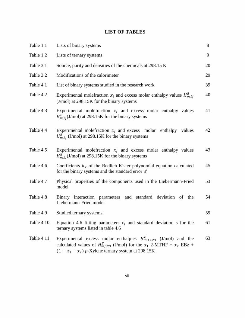
LIST OF TABLES
Table 1.1 Lists of binary systems 8
Table 1.2 Lists of ternary systems 9
Table 3.1 Source, purity and densities of the chemicals at 298.15 K 20
Table 3.2 Modifications of the calorimeter 29
Table 4.1 List of binary systems studied in the research work 39
Table 4.2 Experimental molefraction and excess molar enthalpy values
(J/mol) at 298.15K for the binary systems
40
Table 4.3 Experimental molefraction and excess molar enthalpy values
(J/mol) at 298.15K for the binary systems
41
Table 4.4 Experimental molefraction and excess molar enthalpy values
(J/mol) at 298.15K for the binary systems
42
Table 4.5 Experimental molefraction and excess molar enthalpy values
(J/mol) at 298.15K for the binary systems
43
Table 4.6 Coefficients of the Redlich Kister polynomial equation calculated
for the binary systems and the standard error 's'
45
Table 4.7 Physical properties of the components used in the Liebermann-Fried
model
53
Table 4.8 Binary interaction parameters and standard deviation of the
Liebermann-Fried model
54
Table 4.9 Studied ternary systems 59
Table 4.10 Equation 4.6 fitting parameters and standard deviation s for the
ternary systems listed in table 4.6
61
Table 4.11 Experimental excess molar enthalpies (J/mol) and the
calculated values of (J/mol) for the 2-MTHF + EBz +
p-Xylene ternary system at 298.15K
63
viii
Table 4.12 Experimental excess molar enthalpies (J/mol) and the
calculated values of (J/mol) for the 2-MTHF + EBz +
Mesitylene ternary system at 298.15K
66
Table 4.13 Experimental excess molar enthalpies (J/mol) and the
calculated values of (J/mol) for the 2-ME + EBz +
Mesitylene ternary system at 298.15K
69
Table 4.14 Experimental excess molar enthalpies (J/mol) and the
calculated values of (J/mol) for the 2-ME + 2-MTHF +
p-Xylene ternary system at 298.15K
72
Table 4.15 Experimental excess molar enthalpies (J/mol) and the
calculated values of (J/mol) for the 1-Butanol +
Mesitylene + p-Xylene ternary system at 298.15K
75
Table 4.16 Experimental excess molar enthalpies (J/mol) and the
calculated values of (J/mol) for the 1-Butanol + DNBE +
Mesitylene ternary system at 298.15K
78
Table 4.17 Experimental excess molar enthalpies (J/mol) and the
calculated values of (J/mol) for the 1-Butanol + 2-MTHF
+ EBz ternary system at 298.15K
81
Table 4.18 Experimental excess molar enthalpies (J/mol) and the
calculated values of (J/mol) for the DNBE + 2-MTHF +
EBz ternary system at 298.15K
84
Table 4.19 Experimental excess molar enthalpies (J/mol) and the
calculated values of (J/mol) for the DNBE + 2-MTHF +
EBz ternary system at 298.15K
87
Table 4.20 Standard deviation 's' for the ternary enthalpy values predicted by the
Liebermann-Fried model.
90
Table A1.1 Pump A calibration results 106
Table A1.2 Pump B calibration results 108
Table A1.3 Pump Constant 𝑝 comparison 110
Table B1.1 Pure component properties 112
ix
Table B1.2 Calibration results of DNBE in pump A 112
Table B1.3 Calibration results of 2-MTHF in pump B 114
Table B1.4 Experimental data of the DNBE (1) + 2-MTHF binary system 116
Table B2.1 Ambient conditions and pure component properties for preparing EBz
(1) + p-Xylene (2) mixture of molefraction 0.2500
126
Table B2.2 Summary of weighing 126
Table C1.1 Summary of F statistical test 131
Table D1.1 Motor speed settings for different molefraction of 1-Butanol (1) + p-
Xylene (2) mixing run
162
x
LIST OF FIGURES
Figure 3.1 (Hassan, 2010) Schematic diagram of Vacuum pump degassing
method
22
Figure 3.2
Modified from (Hassan, 2010), schematic representation of LKB flow
microcalorimeter (10700-1)
24
Figure 3.3 Schematic diagram of the calorimeter unit, (Hassan, 2010)
25
Figure 3.4 Schematic diagram of pump control system
27
Figure 3.5 Calibration circuit diagram, (Hassan, 2010)
31
Figure 3.6 Deviations of the excess molar enthalpy at 298.15K for Ethanol (1) +
n-Hexane (2) plotted against molefraction .
33
Figure 4.1 Excess molar enthalpies, for the binary systems presented in
Table 4.2 at 298.15K
46
Figure 4.2 Excess molar enthalpies, for the binary systems at presented in
Table 4.3 at 298.15 K.
47
Figure 4.3 Excess molar enthalpies, for the binary systems presented in
Table 4.4 at 298.15 K.
48
Figure 4.4 Excess molar enthalpies, or the binary systems presented in
Table 4.5 at 298.15 K.
49
Figure 4.5 Excess molar enthalpies, representation by the Liebermann-
Fried model for the binary systems presented in Table 4.2 at 298.15 K
55
Figure 4.6 Excess molar enthalpies, representation by the Liebermann-
Fried model for the binary systems presented in Table 4.3 at 298.15 K
56
Figure 4.8 Excess molar enthalpies, representation by the Liebermann-
Fried model for the binary systems presented in Table 4.5 at 298.15K
58
Figure 4.9
Excess molar enthalpies, for the ternary system 2-MTHF
+ EBz + p-Xylene at 298.15 K.
64
xi
Figure 4.10 Constant enthalpy contours, (J/mol) at 298.15 K for the 2-
MTHF + EBz + p-Xylene, calculated from the
representation of the experimental results using the equation 2.3 and
2.4
65
Figure 4.11 Excess molar enthalpies, for the ternary system 2-MTHF
+ EBz + Mesitylene at 298.15 K
67
Figure 4.12 Constant enthalpy contours, (J/mol) at 298.15 K for the 2-
MTHF + EBz + Mesitylene, calculated from the
representation of the experimental results using the equation 2.3 and
2.4
68
Figure 4.13 Excess molar enthalpies, for the ternary system 2-ME +
EBz + Mesitylene at 298.15 K
70
Figure 4.14 Constant enthalpy contours, (J/mol) at 298.15 K for the 2-
ME + EBz + Mesitylene, calculated from the
representation of the experimental results using the equation 2.3 and
2.4
71
Figure 4.15 Excess molar enthalpies for the ternary system 2-ME +
2-MTHF + p-Xylene at 298.15 K
73
Figure 4.16 Constant enthalpy contours, (J/mol) at 298.15 K for the 2-
ME + 2-MTHF + p-Xylene, calculated from the
representation of the experimental results using the equation 2.3 and
2.4.
73
Figure 4.17 Excess molar enthalpies, for the ternary system 1-Butanol
+ Mesitylene + p-Xylene at 298.15 K
76
Figure 4.19 Excess molar enthalpies, for the ternary system 1-Butanol
+ DNBE + Mesitylene at 298.15 K
79
Figure 4.20 Constant enthalpy contours, (J/mol) at 298.15 K for the 1-
Butanol + DNBE + Mesitylene, calculated from the
representation of the experimental results using the equation 2.3 and
2.4
80
Figure 4.21 Excess molar enthalpies, for the ternary system 1-Butanol
+ 2-MTHF + EBz at 298.15 K.
82
xii
Figure 4.22 Constant enthalpy contours, (J/mol) at 298.15 K for the 1-
Butanol + 2-MTHF + EBz, calculated from the
representation of the experimental results using the equation 2.3 and
2.4
83
Figure 4.23 Excess molar enthalpies, for the ternary system DNBE +
2-MTHF + EBz at 298.15 K
85
Figure 4.24 Constant enthalpy contours, (J/mol) at 298.15 K for the
DNBE + 2-MTHF + EBz, calculated from the
representation of the experimental results using the equation 2.3 and
2.4
86
Figure 4.25 Excess molar enthalpies, for the ternary system DNBE +
Mesitylene + p-Xylene at 298.15 K
88
Figure 4.26 Constant enthalpy contours, (J/mol) at 298.15 K for the
DNBE + Mesitylene + p-Xylene, calculated from the
representation of the experimental results using the equation 2.3 and
2.4
89
Figure A1.1 Pump A calibration plot. Volumetric flow rate Q against motor speed
R
107
Figure A1.2 Pump B calibration plot. Volumetric flow rate Q against motor speed
R.
109
Figure B1.1 Calibration curve for DNBE in pump A
113
Figure B1.2 Calibration curve for 2-MTHF in pump B
115
Figure C2.1 Excess molar enthalpies, for the ternary system 2-MTHF
+ EBz + p-Xylene at 298.15 K. (Liebermann-Fried
model representation)
132
Figure C2.2
Constant enthalpy contours, (J/mol) at 298.15 K for the 2-
MTHF + EBz + p-Xylene, calculated from the
representation of the experimental results using the Liebermann-Fried
model.
133
xiii
Figure C2.3 Excess molar enthalpies, for the ternary system 2-MTHF
+ EBz + Mesitylene at 298.15 K. (Liebermann-Fried
model representation)
134
Figure C2.4 Constant enthalpy contours, (J/mol) at 298.15 K for the 2-
MTHF + EBz + Mesitylene, calculated from the
representation of the experimental results using the Liebermann-Fried
model.
135
Figure C2.5 Excess molar enthalpies, for the ternary system 2-ME +
EBz + Mesitylene at 298.15 K. (Liebermann-Fried
model representation)
136
Figure C2.6 Constant enthalpy contours, (J/mol) at 298.15 K for the 2-
ME + EBz + Mesitylene, calculated from the
representation of the experimental results using the Liebermann-Fried
model
137
Figure C2.7 Excess molar enthalpies, for the ternary system 2-ME +
2-MTHF + p-Xylene at 298.15 K. (Liebermann-Fried
model representation)
138
Figure C2.8 Constant enthalpy contours, (J/mol) at 298.15 K for the 2-
ME + 2-MTHF + p-Xylene, calculated from the
representation of the experimental results using the Liebermann-Fried
model.
139
Figure C2.9 Excess molar enthalpies, for the ternary system 1-Butanol
+ Mesitylene + p-Xylene at 298.15 K. (Liebermann-
Fried model representation)
140
Figure C2.10 Constant enthalpy contours, (J/mol) at 298.15 K for the 1-
Butanol + Mesitylene + p-Xylene, calculated from the
representation of the experimental results using the Liebermann-Fried
model
141
Figure C2.11
Excess molar enthalpies, for the ternary system 1-Butanol
+ DNBE + Mesitylene at 298.15 K. (Liebermann-
Fried model representation)
142
xiv
Figure C2.12 Constant enthalpy contours, (J/mol) at 298.15 K for the 1-
Butanol + DNBE + Mesitylene, calculated from the
representation of the experimental results using the Liebermann-Fried
model.
143
Figure C2.13 Excess molar enthalpies, for the ternary system 1-Butanol
+ 2-MTHF + EBz at 298.15 K. (Liebermann-Fried
model representation)
144
Figure C2.14 Constant enthalpy contours, (J/mol) at 298.15 K for the 1-
Butanol + 2-MTHF + EBz, calculated from the
representation of the experimental results using the Liebermann-Fried
model.
145
Figure C2.15 Excess molar enthalpies, for the ternary system DNBE +
2-MTHF + EBz at 298.15 K. (Liebermann-Fried
model representation)
146
Figure C2.16 Constant enthalpy contours, (J/mol) at 298.15 K for the
DNBE + 2-MTHF + EBz, calculated from the
representation of the experimental results using the Liebermann-Fried
model.
147
Figure C2.17 Excess molar enthalpies, for the ternary system DNBE +
Mesitylene + p-Xylene at 298.15 K. (Liebermann-
Fried model representation)
148
Figure C2.18 Constant enthalpy contours, (J/mol) at 298.15 K for the 1-
Butanol + Mesitylene + p-Xylene, calculated from the
representation of the experimental results using the Liebermann-Fried
model.
149
Figure D1.1 Flow control valve
152
Figure D1.2 Glass syringe connected to pump B outlet tube
153
Figure D1.3 Calorimeter software 154
Figure D1.4 Motor gear position 158
xv
LIST OF ABBREVIATIONS
2-MTHF 2-Methyltetrahydrofuran
2-ME 2-Methoxyethanol
CEPA Canadian Environmental Protection Agency
DNBE Di-n-butyl ether
DSC Differential Scanning Calorimeter
EBZ Ethylbenzene
MTBE Methyl Tertiary Butyl Ether
NRTL Non Random Two liquids
PFG Precision frequency generator
UNIQUAC Universal Quasi Chemical
xvi
NOMENCLATURE
ALPHABETS Unit
A Liebermann-Fried model parameter
c Ternary parameter
E Voltage reading volt (v)
F F statistical test parameter
f Molar flow rate mol/sec
G Gibbs free energy J/mol
G Motor gear ratio
H Excess molar enthalpy J/mol
h Redlich - Kister polynomial coefficient
I Current ampere (A)
I Expression used in equation 4
K Pump calibration constant cm3/sec
M Molecular weight g/mol
m mass of substance gram (g)
N Number of components
n Number of data points
P Pressure kPa
p Parameter number
Q Volumetric flow rate cm3/sec
R Universal gas constant J/mol K
r Electrical resistance ohm (Ω)
xvii
S Entropy J/mol K
s Standard error
T Temperature Kelvin (K)
t Temperature °C
V Volume cm3
x Apparent molefraction component
GREEK LETTERS
α Isobaric thermal expansivity K-1
γ Activity coeeficient
ɛ Calibration constant J/v/s
ϕ Volume fraction
ρ Density g/cm3
R Pump controller reading counts/sec
v,l Degrees of freedom
SUPERSCRIPTS
0 Ideal/Baseline
E Excess function
SUBSCIPTS
1,2 Pump indices
i,j,k,p,q Component indices
xviii
A,B Pump notation
cal Calculated values
exp Experimental data
H Humidity
k Parameter indices
M Mixture
m Molar property
p Pump
P Isobaric properties
1
1.0 INTRODUCTION
Declining petroleum resources and increased energy usage and environmental
deterioration forced the nations to make the petroleum refining process efficient, economical,
and environment friendly. During the period from 1915 to the late 1970’s tetraethyllead was
extensively used for its excellent anti-knocking properties which resulted in dramatic
improvement engine efficiency and life. But research conducted through 1960 to 1970 revealed
that using tetraethyllead in gasoline increased the blood lead level, which reflected a detrimental
effect on human health and therefore use of tetraethyllead as a gasoline addictive was banned all
over the world. The gasoline regulations (CEPA, 1990) restricts the use of leaded gasoline in
commercial vehicles in Canada
Phasing out lead as an additive reduced the gasoline’s octane number had affected the
performance of automobiles that were dependent on high-octane fuels. In order to increase the
fuels’ octane ratings, fuel suppliers have used oxygenates namely alcohol and ethers, as fuel
additives. Among the oxygenates, methyl tertiary butyl ether (MTBE) showed a superior
performance as an octane enhancer and greatly reduced the emission of atmospheric pollutants
like carbon monoxide (CO) and volatile organic compounds from the vehicle exhaust. Due to its
low cost, its ease of production, and the favorable transfer and blending characteristics, MTBE
was produced and used worldwide as oxygenated gasoline additive since 1973 (30 million
tons/year in 1995) (Ancillotti and Fattore, 1998).
2
In early 2000s, studies revealed that in many places in the United States MTBE caused
serious health issues including the risk of cancer on long term exposure (Davis and Farland,
2001). Thereafter, research work focused on finding safe, efficient and economical ether and
alcohols to blend with gasoline was triggered, and the studies of thermodynamic properties of
mixtures involving hydrocarbons, ethers and alcohol turn out to be essential in design and
operation of separation equipment.
Thermodynamic properties of mixtures involving hydrocarbons, ethers and alcohols are of
fundamental importance in petroleum based applications such as modeling and design of heat
exchangers, reactors and fluid-phase separation equipment. Thermodynamic data for
representative mixtures are useful as the experimentally obtained information will help us to
understand the molecular interactions occurring between the constituent species in liquid
mixtures and to test and validate thermodynamic models.
1.1 Objectives
The study reported in this thesis is a continuation of the research work conducted in the
Applied Thermodynamics Laboratory in the Department of Chemical and Biological
Engineering at the University of Saskatchewan. Hassan (2010) has measured the excess molar
enthalpy of 10 binary and six ternary systems involving hydrocarbons, ethers and alcohols. The
main objectives of my research work are
(1) To measure the enthalpy of mixing for selected binary and ternary systems at fixed
pressure and temperature and
(2) To determine the optimal parameter values for use with selected empirical models to
represent the experimental excess molar enthalpy data for binary and ternary systems
3
In this thesis, the experimental work on the excess molar enthalpy of 16 binary systems and 9
ternary systems involving hydrocarbon and ethers is described. The measured excess molar
enthalpy values of the binary systems are correlated by means of the Redlich – Kister polynomial
equation and the Liebermann-Fried solution theory model, respectively. In addition, a
description of the application of the Tsao-Smith model and the Liebermann – Fried solution
theory to the experimental results obtained for the ternary systems is also presented.
1.2 An overview of the thesis
A literature review is presented in Chapter 2, which serves to describe the methods for
measuring the excess molar enthalpy values and the correlation and prediction methods for
representing the experimental excess molar values.
In Chapter 3 the details of the equipment used, material properties and the experimental
procedures followed in the course of the study will be discussed. In Chapter 4 the experimental
results and discussion are presented.
Chapter 5 concludes the thesis with recommendations for future work.
1.3 Importance of the study
1.3.1 Excess Thermodynamic Properties
An excess property of a solution can be best expressed as the difference between the
actual property values of a solution and the value it would have as an ideal solution at the same
composition, temperature and pressure Smith et al. (2005). Mathematically it can be written as
(1.1)
4
Where is the excess property of the solution and M is the actual property value of the
solution and is the property value as an ideal solution, there are many excess properties of
which following are the most widely studied, which are excess molar enthalpy , excess molar
volume , Excess molar Gibbs energy
, and excess molar entropy . At constant
temperature, pressure excess molar volume and excess molar enthalpy is zero an ideal solution.
(1.2)
(1.3)
Whereas change in Gibbs energy and Entropy for an ideal solution mixture is non-zero and
expressed as
∑ 𝑙𝑛 (1.4)
∑ 𝑙𝑛 (1.5)
The intermolecular forces resulting from the interaction of various species when forming
a liquid mixture are related to the excess thermodynamic properties of the system. Studying
thermodynamic excess properties such as excess molar enthalpy and excess molar volume
provide knowledge about intermolecular forces and molecular interactions in a liquid mixture.
1.3.2 Excess molar enthalpy
The excess molar enthalpy data are the most often measured excess thermodynamic
property since it is relatively easy to obtain and the data can be used to calculate other excess
thermodynamic properties, vapor-liquid equilibrium values and are the observables to determine
5
the intermolecular forces. Heat of mixing is a very essential property in separation processes and
also it determines the variation of activity coefficient with temperature. Activity coefficient is a
very critical parameter considered in the design of chemical processes which involves phase
separation.
*
( )
+
= ∑ *
+
(1.6)
(Zudkevitch, 1978) explained the importance of the heat of mixing values in his review, in which
he reported that a substantial 30% production decline was encountered with unacceptable
product purity during the distillation of cyclohexanone and cyclohexanol. The reason for the
anomaly in the distillation process was due to omitting the heat of mixing values from the
calculation, this example emphasize the significance of heat of mixing data in separation process.
1.4 System studied
In this research work a special attention was paid in choosing the chemicals to study,
Marsh et al. (1999) in their paper listed the works of various researchers on thermophysical
properties of binary and ternary mixtures involving oxygenates and hydrocarbons. Upon
reviewing Marsh et al. (1999) paper it was observed that the thermophysical properties of many
potential binary and ternary systems involving hydrocarbons and ethers needs to be studied.
Based on Marsh et al. review seven chemical species were chosen for the study and they are
listed as follows
6
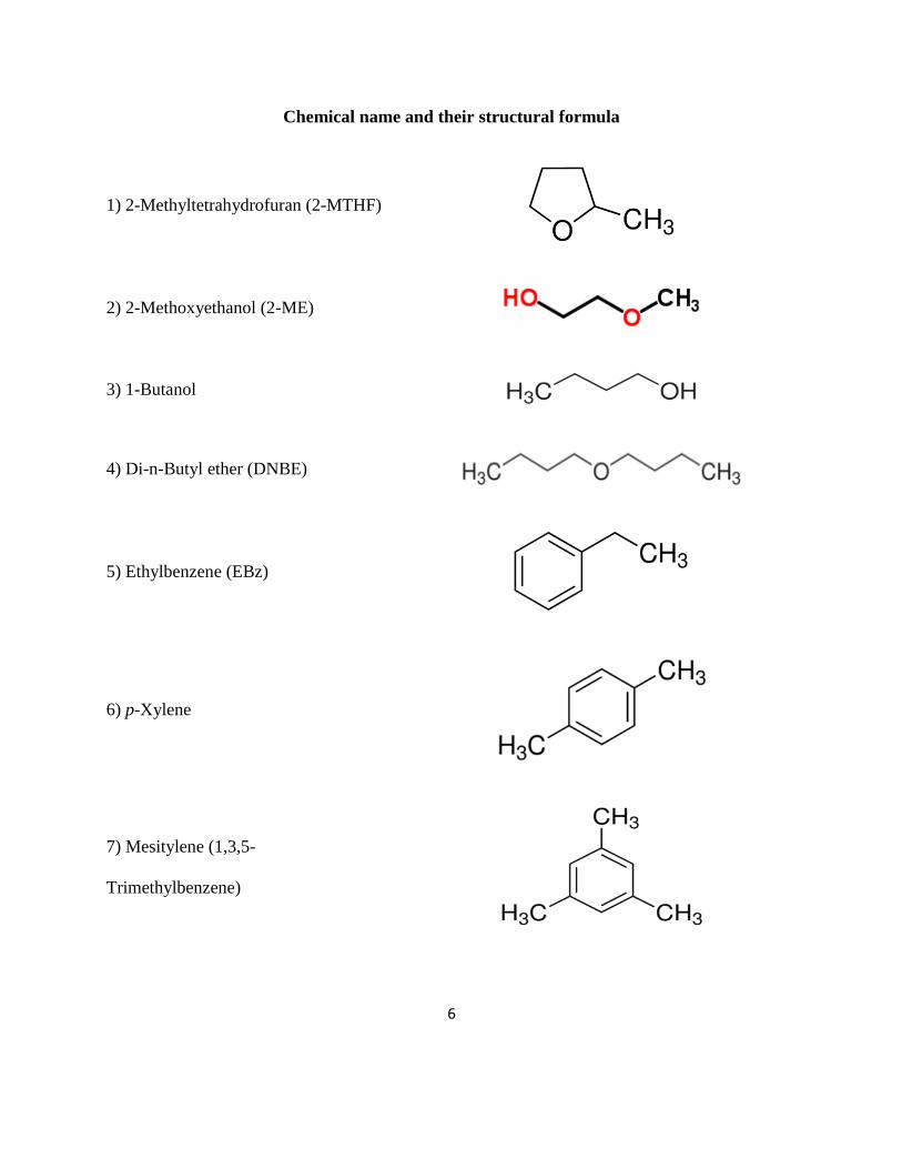
Chemical name and their structural formula
1) 2-Methyltetrahydrofuran (2-MTHF)
2) 2-Methoxyethanol (2-ME)
3) 1-Butanol
4) Di-n-Butyl ether (DNBE)
5) Ethylbenzene (EBz)
6) p-Xylene
7) Mesitylene (1,3,5-
Trimethylbenzene)
7
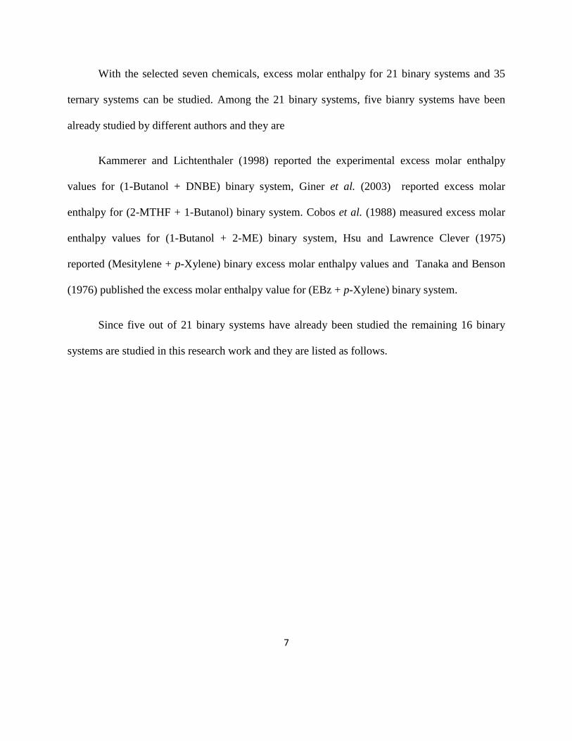
With the selected seven chemicals, excess molar enthalpy for 21 binary systems and 35
ternary systems can be studied. Among the 21 binary systems, five bianry systems have been
already studied by different authors and they are
Kammerer and Lichtenthaler (1998) reported the experimental excess molar enthalpy
values for (1-Butanol + DNBE) binary system, Giner et al. (2003) reported excess molar
enthalpy for (2-MTHF + 1-Butanol) binary system. Cobos et al. (1988) measured excess molar
enthalpy values for (1-Butanol + 2-ME) binary system, Hsu and Lawrence Clever (1975)
reported (Mesitylene + p-Xylene) binary excess molar enthalpy values and Tanaka and Benson
(1976) published the excess molar enthalpy value for (EBz + p-Xylene) binary system.
Since five out of 21 binary systems have already been studied the remaining 16 binary
systems are studied in this research work and they are listed as follows.
8
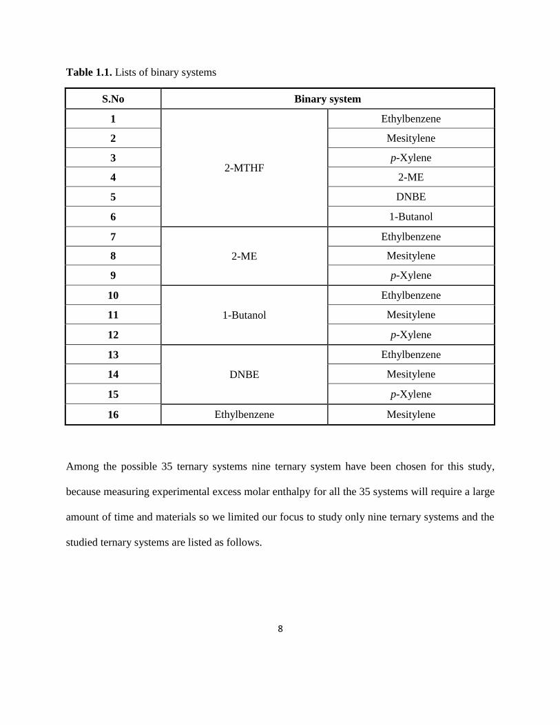
Table 1.1. Lists of binary systems
S.No Binary system
1
2-MTHF
Ethylbenzene
2 Mesitylene
3 p-Xylene
4 2-ME
5 DNBE
6 1-Butanol
7
2-ME
Ethylbenzene
8 Mesitylene
9 p-Xylene
10
1-Butanol
Ethylbenzene
11 Mesitylene
12 p-Xylene
13
DNBE
Ethylbenzene
14 Mesitylene
15 p-Xylene
16 Ethylbenzene Mesitylene
Among the possible 35 ternary systems nine ternary system have been chosen for this study,
because measuring experimental excess molar enthalpy for all the 35 systems will require a large
amount of time and materials so we limited our focus to study only nine ternary systems and the
studied ternary systems are listed as follows.
9
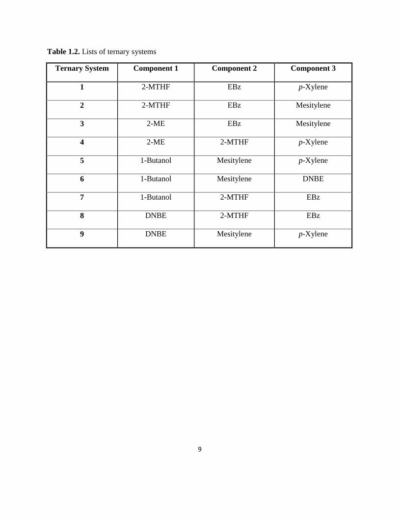
Table 1.2. Lists of ternary systems
Ternary System Component 1 Component 2 Component 3
1 2-MTHF EBz p-Xylene
2 2-MTHF EBz Mesitylene
3 2-ME EBz Mesitylene
4 2-ME 2-MTHF p-Xylene
5 1-Butanol Mesitylene p-Xylene
6 1-Butanol Mesitylene DNBE
7 1-Butanol 2-MTHF EBz
8 DNBE 2-MTHF EBz
9 DNBE Mesitylene p-Xylene
10
2.0 LITERATURE REVIEW
This chapter covers the different calorimetric approach for measuring excess molar
enthalpy values and discusses the different correlation and prediction methods for representing
the experimental excess molar enthalpy values.
2.1 Methods of measuring excess molar enthalpy values
Heat of mixing values can be calculated from using other excess thermodynamic
properties such as excess Gibbs energy, Gibbs-Helmholtz equation (equation 2.1) relates the
excess molar enthalpy and excess Gibbs energy.
(
)
(2.1)
In order to calculate the excess molar enthalpy from the equation 2.1 temperature
derivatives of the excess Gibbs energy is required. But for most systems the excess molar Gibbs
energy and excess molar enthalpy is available only at specific temperatures so calculating excess
properties from equation 2.1 is generally not considered. Thus calorimetric measurement is the
most reliable technique in determining the excess molar enthalpy values.
2.1.1 Calorimetric methods
Any change in the state of a system is accompanied with either loss or gain of energy.
Measuring and studying the energy difference of a system is a source of information for
understanding molecular interactions and molecular structure. Calorimetric method is
undoubtedly the most prevailing and technologically advanced procedure for measuring the
11
excess molar enthalpy of liquid mixtures. In their paper Ott and Sipowska (1996) extensively
covered the different types of calorimeter used for measuring the excess molar enthalpies of non-
electrolyte solutions. Calorimetric attempts to measure the excess molar enthalpy values dates
back more than a century. Researchers like Clarke (1905), Bose (1907), Baud (1915) reported
heats of mixing values for alcohol-water mixtures, hydrocarbon with halogenated mixtures and
aromatic with aliphatic hydrocarbon mixtures. In 1921 Hirobe (1925) published excess molar
enthalpies for 51 binary mixtures using a sophisticated isothermal calorimeter and the deviation
of some of the data published by Hirobe are within few percent of the results obtained with the
best modern calorimeters.
2.1.2 Types of calorimeters
Different types of calorimeters have been developed and used successfully for measuring
excess molar enthalpy values based on different operating conditions. Hassan (2010) in his thesis
described three different kinds of calorimeters operated under normal temperature and pressure
to measure excess molar enthalpy values. They are
1) Isothermal Titration Calorimeter
2) Differential Scanning calorimeter
3) Flow calorimeter
Isothermal Titration Calorimeter
Isothermal titration calorimeters are built on the same conduction principle as flow
calorimeters and the principle involved is that a fixed quantity of component 1 is placed inside a
12
mixing cell and component 2 is injected into the mixing cell either continuously or in fixed
volumes. The prototype of the isothermal titration calorimeter was first designed and developed
by Christensen et al. (1968) and Wadso (1968), further modification of the titration calorimeter
by Holt and Smith (1974) and Rodríguez de Rivera et al. (2009) improved the accuracy of the
results. These calorimeters are widely used for studying the bio-molecular interactions studies
but its application in measuring the excess molar enthalpy values is less pronounced. Liao et al.
(2009a, 2009b, 2012) used isothermal titration for measuring binary excess molar enthalpies of
various mixtures involving hydrocarbons, ether, alcohol and acids and reported higher accurate
results.
Differential Scanning Calorimeter (DSC)
The Differential scanning calorimeter is a versatile instrument for direct assessment of
change in heat energy of a system. DCS is measure of change of difference in the heat flow rate
to the sample and to a reference sample while they are subjected to a controlled temperature
program Höhne et al. (2003). The DSC measures the excessive heat quantity released or
absorbed by a sample on the basis of temperature difference between the sample and a reference
material Gill et al. (2010). Differential scanning calorimeter is commonly used for biochemical
reactions, and also for thermal transition and reactions, crystallization, oxidation, fusion, heat of
reaction and heat capacity measurements. Even though the DSC are not widely used for heat of
mixing measurements Jablonski et al. (2003) showed that the DSC are a potential tool for heat of
mixing measurements.
13
2.2 Flow calorimeters
In recent years flow calorimetry has been the preferred method for researchers to measure
the heat effects during mixing process. Flow calorimeters have distinct advantages over batch
and isothermal displacement calorimeters, for example when relative volatiles are involved,
formation of vapor-phase is a serious problem and leads to large errors in batch calorimeter.
Flow calorimeters can be used to measure
i. Excess molar enthalpy values under wide range of pressure and temperature
conditions, for both gas and liquid components
ii. Studies involving corrosive and reactive chemicals where the batch and isothermal
displacement calorimeter cannot be used.
In flow calorimeter two different working fluids mixes in a mixing cell at steady state
with fixed flow rates. The flow rates can be adjusted to measure heat of mixing values at wide
range of composition with high precision. Monk and Wadsö (1968) designed and tested the
prototype of the flow reaction calorimeter and showed the advantages of using flow calorimeter
over batch calorimeter. Flow calorimeters of different types have been successfully designed and
used by many researchers for measuring excess molar enthalpy values at various pressure and
temperature conditions, namely Picker (1974), Wormald and colleagues, Elliott and Wormald,
(1976), Wormald et al. (1977), and Christensen and co-workers Christensen et al. (1976).
Tanaka et al. (1975) modified the design of Monk and Wadso's flow calorimeter and
measured the excess molar enthalpy values for non-electrolytes with higher accuracy. Later
14
Kimura et al. (1983) reported a 0.5% increased accuracy in his work by modifying the operating
techniques of the flow calorimeter.
One of the few setbacks of flow calorimeter is it requires large amount of chemicals to
measure the excess molar enthalpy values so for measurements involving rare and expensive
components calorimeters are not the best choice. Regardless of the drawback flow calorimeter's
numerous successful measurements ensured a prominent position in the scientific community to
justify its usage. Choosing the right calorimeter depends on the requirements of the specific
research field, if the measurement especially involves heat of mixing values for multicomponent
systems a flow calorimeter would be the right choice, while a batch calorimeter would be much
suitable for measurements involving chemical reactions and biological processes.
2.3 Correlation and prediction methods
The synthesis of chemical compounds, design of separation process, solvent selection and
ideal operating conditions needs a reliable knowledge of phase equilibrium behavior of a fluid
mixture as a function of temperature, pressure and composition. A thermodynamic model
describes the real fluid mixture behavior using the existing experimental data and pure
component properties.
Correlation and prediction methods are always an interesting topic among researchers in
the experimental thermodynamics field, with the scope of avoiding time consumption and
difficulties encountered in the experimental measurement of excess enthalpies especially for the
multicomponent mixtures. Among the correlation and prediction methods some of them are
mathematical expressions and some of them are theoretical models.
15
2.3.1 Empirical methods
Empirical expressions are the mathematical models which are very useful and convenient
for data correlation. These models have parameters in their formula which is fitted to the
experimental data, the best fit of parameters and quality of the representation was judged by the
standard deviation. The empirical expressions have limitations, for example the model with
highest number of adjustable parameters doesn't necessarily means it is the excellent
representation of the experimental data.
2.3.1.1 The Redlich - Kister polynomial equation
Redlich and Kister described an expression which is the most widely used polynomial
equation to represent binary excess molar enthalpy data. The other notable mathematical models
used for representing experimental excess molar enthalpies are the expressions given by
Brandreth et al. (1966), Mrazek and Van Ness (1961), Rogalski and Malanowski (1977) SSF
equation and Wilson's equation. Prchal et al. (1982) reviewed the mathematical models used for
representing the binary experimental excess molar enthalpy values and in their paper they found
that the Redlich-Kister model best describes the binary experimental heat of mixing values.
Redlich-Kister assumed a particular form of enthalpy values (HE) as a function of mole fraction
( ) with one or more adjustable parameters and the parameters are chosen by the method of least
square to minimize the error in (HE).
Ternary excess molar enthalpy data can be represented through empirical expressions, one
of the widely used empirical equations for representing ternary excess molar enthalpy with high
accuracy is the one proposed by Tsao and Smith (1953) with an added ternary term defined by
16
Morris et al. (1975) The Redlich - Kister expression and the Tsao and Smith expression for
representing the binary and ternary experimental excess molar enthalpy values are discussed in
detail in chapter 4.
2.3.2 Solution theory models
An interesting approach to represent excess enthalpy values is by means of local
composition models like the Wilson equation (Wilson, 1964) , the NRTL equation (Renon and
Prausnitz, 1968), and the UNIQUAC model (Abrams and Prausnitz, 1975) and other solution
theory models such as the Flory theory Flory (1965) Abe and Flory (1965) and the Liebermann-
Fried model Liebermann and Fried (1972a,b). Even though the solution theory models are still at
semi-empirical to empirical stage, it correlates and predict binary and multicomponent excess
molar enthalpy values with reliable accuracy and the solution theory models are widely used
with one or more parameters fitted to the experimental data.
The model proposed by Van Laar in 1906 is based on inserting the van der Waals
equation into the thermal equation of state for a proposed thermodynamically reversible mixing
process. The assumptions used involved that, for a binary mixture consisting of two species of
similar size and same energies of interaction, the molecules of each species are uniformly
distributed throughout the mixture and that the van der Waals equation of state is applicable to
both of the pure liquids and the resulting liquid mixture.
At a given temperature and pressure and
17
The solution theory assumes that mixture interactions were independent of each other and
quadratic mixing rules would provide reasonable approximations. The regular solution models
are based on random mixing of molecules but the mixing of molecules is not really random due
to the intermolecular forces. This draw back of the regular solution models was later overcome
by Wilson model based on the local composition concept.
Models based on the Local composition concept
Wilson in 1964 came up with his much acclaimed Gibbs free energy equation based on
the local composition model in which he explained that mixing of molecules are not completely
random and explained that specific molecular interactions are due to intermolecular forces
between the molecules. Wilson model is capable of representing the behavior of multicomponent
system using only the binary system parameters. A drawback of the Wilson model is that it
cannot handle liquid - liquid immiscibility.
Other widely known models which are based on local composition concept are the NRTL
(Non Random Two Liquids) proposed by Renon and Prausnitz in 1968 and the UNIQUAC
(Universal Quasi Chemical) model proposed by Abrams and Prausnitz in 1975. The NRTL was
proven to predict and correlate experimental data with high accuracy. NRTL can be used to
predict and correlate enthalpy data for liquid-liquid immiscible systems unlike Wilson's model.
The original NRTL model has been modified by many authors and was used to predict excess
properties for electrolytes, polar and non-polar systems.
Universal Quasi-Chemical or UNIQUAC model was developed by Abrams and Prausnitz
(1975) in their model they adopted the two-liquid model and the local composition model. They
18
assumed that the activity coefficient expression consists of two parts, the combinatorial part
which is due to the size difference and shape of the molecules, and the residual part which is due
to the energetic interactions. UNIQUAC can be applied to multicomponent mixtures in terms of
binary parameters, liquid-liquid equilibrium, and representation of systems with widely different
molecular sizes.
Based on the partition functions Flory derived a liquid equation of state which relates to
the excess functions of the mixture. The Flory theory was developed for the correlation of
thermodynamic properties of long chain liquid molecules and liquid mixtures, then later
modified from its original form and applied to calculate one excess thermodynamic property
from other excess thermodynamic property and also to calculate excess properties of systems
involving small non-polar molecules. The Flory theory is widely praised for its simplicity in
determining the model parameters from the physical properties of the pure components like
isobaric expansivity , isothermal compressibility and the interchange energy parameter
which is calculated by regression of the experimental values.
2.3.2.1 Liebermann - Fried model
Liebermann and Fried Gibbs free energy model has two parts, one part represents the
contribution due to the intermolecular forces and the other part reflects the contribution due to
the difference in the size of the molecules. Wang and Lu (2000) used the Liebermann-Fried
Gibbs energy model and successfully predicted the isobaric VLE values for Methyl tert butyl
ether - alkanes system using excess enthalpy data determined at a different temperature. Peng et
al. (2001) used the Liebermann-Fried model to correlate the excess enthalpy values of
19
hydrocarbon + ether binary systems and used the parameters obtained from that correlation to
predict the excess enthalpies and VLE values for several multicomponent systems. Wang et al.
(2005) used the excess molar enthalpy values for 123 binary mixtures at 298.15K from the
literature and calculated the Liebermann-Fried binary interaction parameters for those 123
mixtures. Using those parameters the VLE values for the respective binary systems with
reasonable accuracy was reported. Detailed explanation of the Liebermann-Fried model is
discussed in chapter 4.
20
3.0 MATERIALS AND METHODS
3.1 Materials
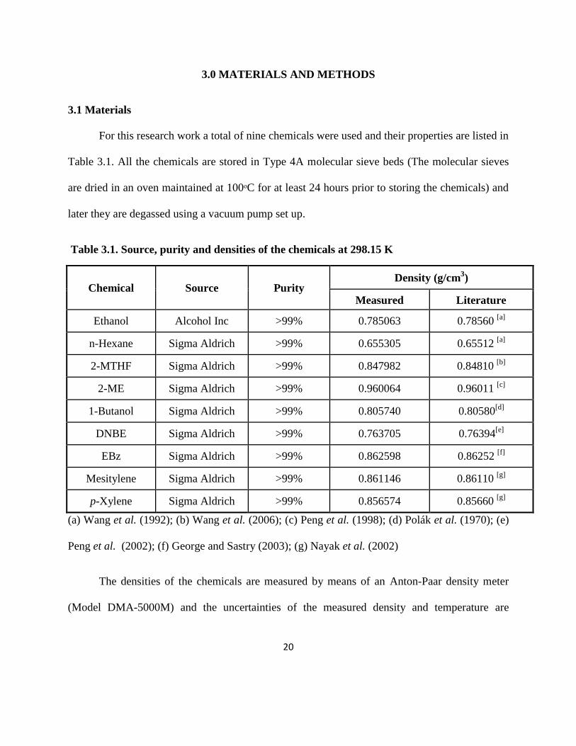
For this research work a total of nine chemicals were used and their properties are listed in
Table 3.1. All the chemicals are stored in Type 4A molecular sieve beds (The molecular sieves
are dried in an oven maintained at 100ᵒC for at least 24 hours prior to storing the chemicals) and
later they are degassed using a vacuum pump set up.
Table 3.1. Source, purity and densities of the chemicals at 298.15 K
Chemical Source Purity Density (g/cm
3)
Measured Literature
Ethanol Alcohol Inc >99% 0.785063 0.78560 [a]
n-Hexane Sigma Aldrich >99% 0.655305 0.65512 [a]
2-MTHF Sigma Aldrich >99% 0.847982 0.84810 [b]
2-ME Sigma Aldrich >99% 0.960064 0.96011 [c]
1-Butanol Sigma Aldrich >99% 0.805740 0.80580[d]
DNBE Sigma Aldrich >99% 0.763705 0.76394[e]
EBz Sigma Aldrich >99% 0.862598 0.86252 [f]
Mesitylene Sigma Aldrich >99% 0.861146 0.86110 [g]
p-Xylene Sigma Aldrich >99% 0.856574 0.85660 [g]
(a) Wang et al. (1992); (b) Wang et al. (2006); (c) Peng et al. (1998); (d) Polák et al. (1970); (e)
Peng et al. (2002); (f) George and Sastry (2003); (g) Nayak et al. (2002)
The densities of the chemicals are measured by means of an Anton-Paar density meter
(Model DMA-5000M) and the uncertainties of the measured density and temperature are
21
±0.000005 g/cm3 and ±0.001ᵒC, respectively. These uncertainty values are provided by the
density meter manufacturer.
3.1.1 Degassing the chemicals
The removal of dissolved gases from aqueous phase is an important process in many
applications and it is carried out by different techniques namely pressure reduction,
heating, membrane degasification and Inert gas substitution. Gas removal from liquids is
very vital for carrying out excess molar enthalpy measurements. In particular using the
degassed pure liquids helped to prevent the bubble formation in the mixing cell Tanaka et
al. (1975). In this study all the pure component liquids are degassed using a vacuum pump
setup figure 3.1.
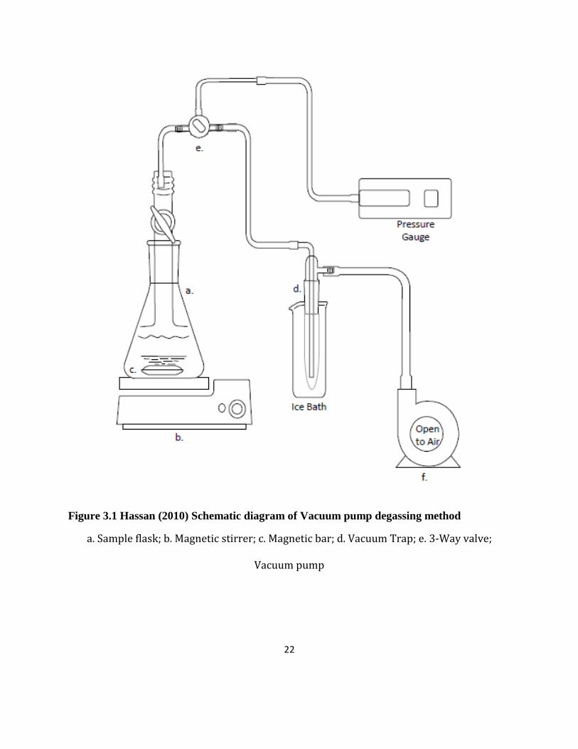
A conical flask (a) with the pure component liquid and a magnetic bar (c) is placed on
a magnetic stirrer (b) which agitates the liquid. The outlet of the flask was connected to a
vacuum pump (f) through a three way valve (e), when the vacuum pump is turned on it
creates a negative pressure inside the system which in turn evacuates the dissolved gas in
the liquid. The agitation helps in removing the gas at a faster rate and the loss of pure
component as vapor was prevented by condensing the vapor, the condensation was
achieved by using a vapor trap (d) placed inside an ice bath. The degassing process was
carried out until the bubbles stops appearing from the pure component liquid and the
process take about five to ten minutes for each pure component.
22
Figure 3.1 Hassan (2010) Schematic diagram of Vacuum pump degassing method
a. Sample flask; b. Magnetic stirrer; c. Magnetic bar; d. Vacuum Trap; e. 3-Way valve;
Vacuum pump
23
3.2 Flow microcalorimeter
An LKB 10700-1 flow microcalorimeter is used in this research work and the prototype of
this calorimeter is the one which Monk and Wadsö (1968) used for determining the heat of
dilution of aqueous electrolyte. Harsted and Thomsen (1974) reviewed the calorimeter prototype
and made some modifications to the Monk and Wadsö (1968) model and achieved more accurate
results. Later Tanaka et al. (1975) made several changes in the operating techniques which are as
follows
i. Degassing the chemicals,
ii. Modification of the auxiliary parts namely using large cooling coils for an improved air
bath temperature control.
iii. Digitalized measurement of the thermopile response and calibration heater circuit current
and a modified pump construction for satisfactory flow system.
Kimura et al. (1983) achieved more accurate excess molar enthalpy measurements with further
modifications in the calorimeter operating techniques.
24
3.2.1 Calorimeter construction and modifications.
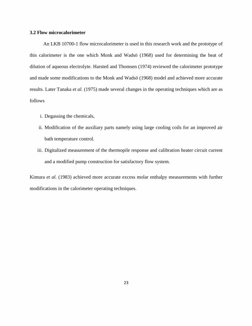
The figure below is the schematic representation of the LKB-Flow microcalorimeter
(Model 10700-1)
Figure 3.2. Modified from Hassan (2010), schematic representation of LKB flow
microcalorimeter (10700-1)
25
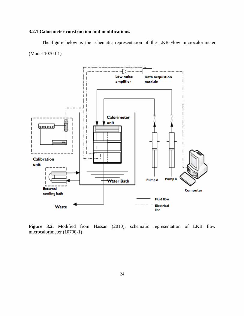
The calorimeter unit (Figure 3.3) consists of two compartments: one is a mixing cell and
another is a reference cell. The cells are enclosed in a heat sink and sandwiched between two
thermopiles (thermocouples connected in series), the thermopiles are placed in a close contact
with the mixing cell and a calorimeter calibration heater circuit is connected to this unit. The
calibration heater circuit consists of a DC power supply along with a standard resistance (10 Ώ)
connected to the calibration heater.
Figure 3.3. Schematic diagram of the calorimeter unit, (Hassan, 2010)
The calorimeter is placed in a constant temperature water bath, whose temperature is
controlled by a heater (PF Hetotherm) and a coolant (VWR temperature controller) unit. The
temperature of the water bath is maintained at ±0.005 and it is monitored by a thermometer
(HP, Model-2804A).
26
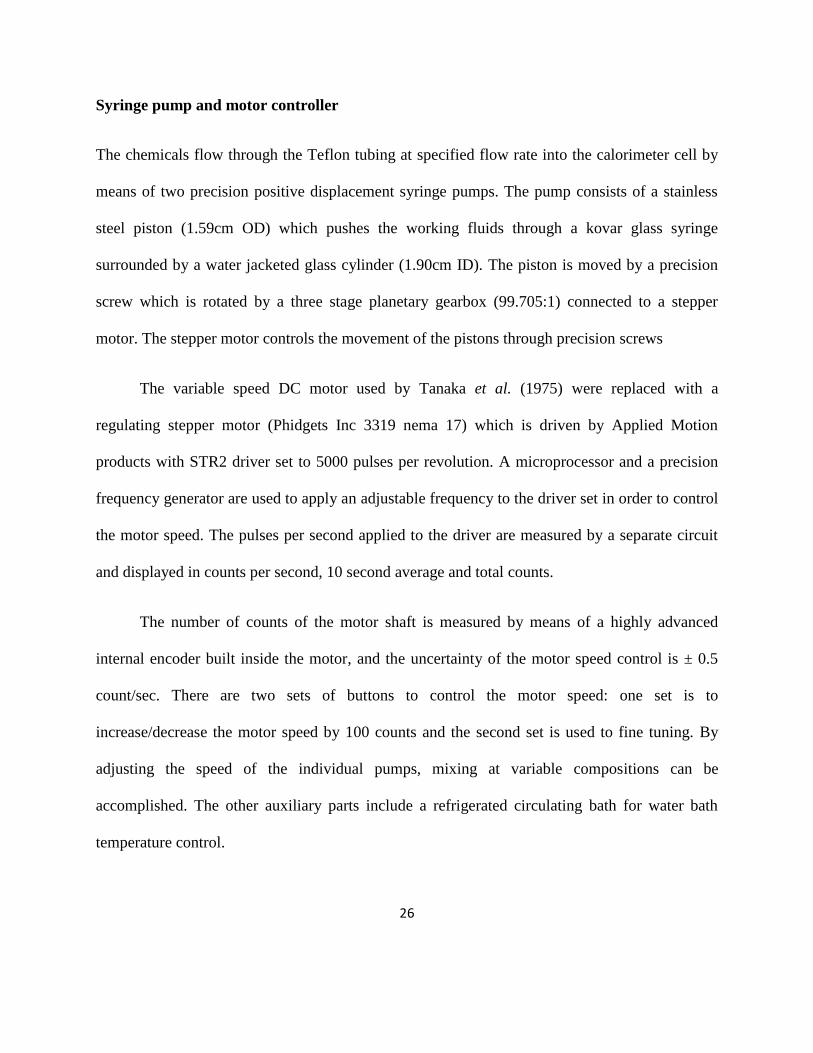
Syringe pump and motor controller
The chemicals flow through the Teflon tubing at specified flow rate into the calorimeter cell by
means of two precision positive displacement syringe pumps. The pump consists of a stainless
steel piston (1.59cm OD) which pushes the working fluids through a kovar glass syringe
surrounded by a water jacketed glass cylinder (1.90cm ID). The piston is moved by a precision
screw which is rotated by a three stage planetary gearbox (99.705:1) connected to a stepper
motor. The stepper motor controls the movement of the pistons through precision screws
The variable speed DC motor used by Tanaka et al. (1975) were replaced with a
regulating stepper motor (Phidgets Inc 3319 nema 17) which is driven by Applied Motion
products with STR2 driver set to 5000 pulses per revolution. A microprocessor and a precision
frequency generator are used to apply an adjustable frequency to the driver set in order to control
the motor speed. The pulses per second applied to the driver are measured by a separate circuit
and displayed in counts per second, 10 second average and total counts.
The number of counts of the motor shaft is measured by means of a highly advanced
internal encoder built inside the motor, and the uncertainty of the motor speed control is ± 0.5
count/sec. There are two sets of buttons to control the motor speed: one set is to
increase/decrease the motor speed by 100 counts and the second set is used to fine tuning. By
adjusting the speed of the individual pumps, mixing at variable compositions can be
accomplished. The other auxiliary parts include a refrigerated circulating bath for water bath
temperature control.
27
Figure 3.4. Schematic diagram of pump control system (Courtesy: Rlee Prokopishyn)
Mixing of fluids and data acquisition
The working fluids are initially degassed by means of vacuum pump system in order to
avoid gas bubble formation during the mixing run. The fluids are conveyed into the mixing cell
at specific flow rate by means of the pumps running at specific speed. Before reaching the
28
mixing cell the fluids are brought to the working temperature through the temperature control
system consisting of heat exchangers. Heat arising from the mixing of the fluids is transported
from the mixing cell to the surrounding thermopile by heat conduction. The thermopile reflects
this temperature as electrical signals and these signals are processed by a data acquisition system
which consists of an amplifier, a digital signal converter (National instruments USB 6008
acquisition model) and a computer software (National instrument labview 8.5.1 software). The
electrical signals are amplified by the amplifier, the amplifier does a differential amplification up
to 2500 times and the amplified signals are fed into a Digital signal converter which converts the
amplified signal into a digital signal and finally the digitalized signal is fed into the computer.
Through the software, this digitalized signal is observed as the real time thermopile voltage and
it is recorded at fixed intervals and an average of 100 data points was taken as the final voltage
of the mixture .
29
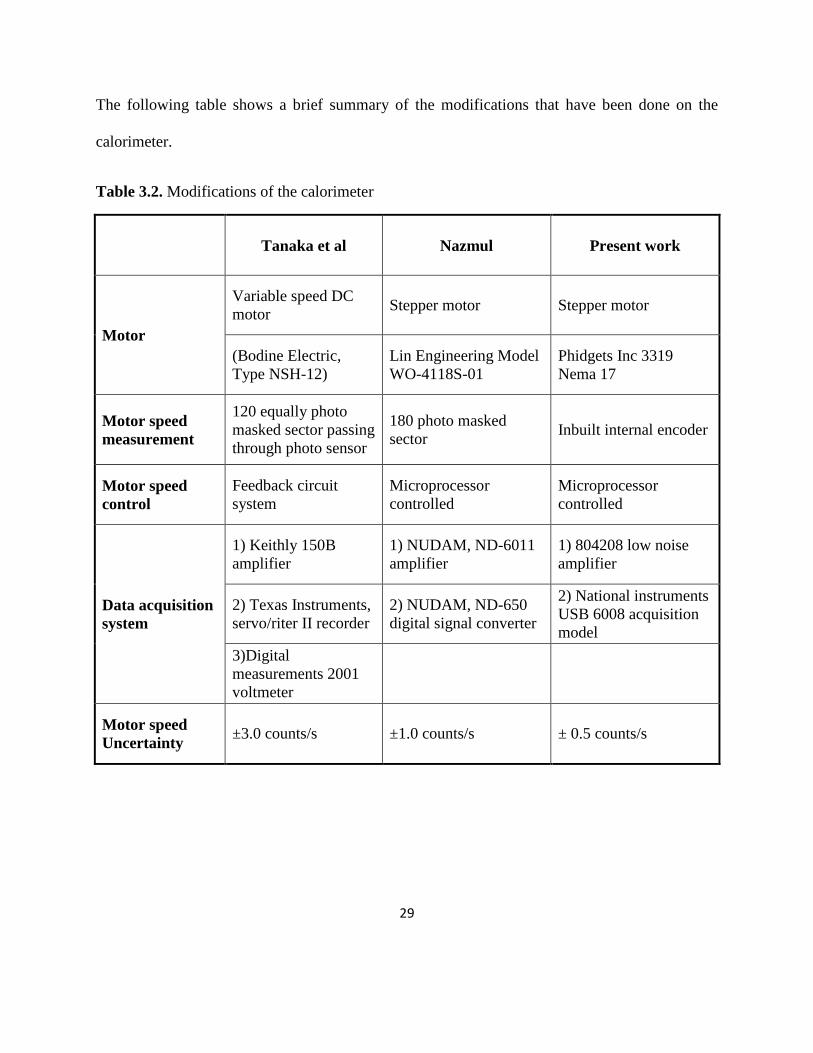
The following table shows a brief summary of the modifications that have been done on the
calorimeter.
Table 3.2. Modifications of the calorimeter
Tanaka et al Nazmul Present work
Motor
Variable speed DC
motor Stepper motor Stepper motor
(Bodine Electric,
Type NSH-12)
Lin Engineering Model
WO-4118S-01
Phidgets Inc 3319
Nema 17
Motor speed
measurement
120 equally photo
masked sector passing
through photo sensor
180 photo masked
sector Inbuilt internal encoder
Motor speed
control
Feedback circuit
system
Microprocessor
controlled
Microprocessor
controlled
Data acquisition
system
1) Keithly 150B
amplifier
1) NUDAM, ND-6011
amplifier
1) 804208 low noise
amplifier
2) Texas Instruments,
servo/riter II recorder
2) NUDAM, ND-650
digital signal converter
2) National instruments
USB 6008 acquisition
model
3)Digital
measurements 2001
voltmeter
Motor speed
Uncertainty ±3.0 counts/s ±1.0 counts/s ± 0.5 counts/s
30
3.2.2 Calorimeter Calibration
Calibration is essential for all the type of calorimeters which are used to measure the excess
molar enthalpy values. The calibration step must be performed prior to the mixing run and the
calibration constants should be calculated. The calibration constants relate the thermoelectric output
and the heat effect associated with it when there is no mixing of fluids inside the mixing cell. It is
carried out for individual liquids flowing from each pump into the mixing cell. The calibration is
done by two ways: chemical and electrical. Chemical calibration method was prone to sensitivity
variation Rodríguez de Rivera and Socorro (2007) so in this study the electrical calibration method
was practiced. The working fluids are pumped at specific flow rate and the average baseline voltage
is recorded, now the calibration heater is turned on and the baseline voltage changes and the
average value of the baseline voltage are recorded.
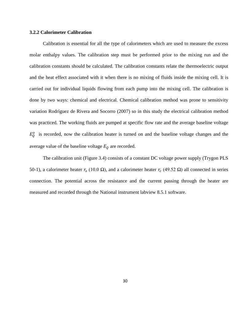
The calibration unit (Figure 3.4) consists of a constant DC voltage power supply (Trygon PLS
50-1), a calorimeter heater 𝑟 (10.0 Ω), and a calorimeter heater 𝑟 (49.52 Ω) all connected in series
connection. The potential across the resistance and the current passing through the heater are
measured and recorded through the National instrument labview 8.5.1 software.
31
Figure 3.5. Calibration circuit diagram, (Hassan, 2010)
The calibration constant is then calculated from the equation
(3.1)
where I is the current flowing through the heater, 𝑟 is the resistance of the heater. A graph is
plotted between the and the motor speed R (counts/sec) and from the plot an expression for
calibration constant in relation with motor speed R (counts/sec) is obtained. This is of the form
𝑘 𝑘 (3.2)
Where k0 and k1 are constants for the given liquid
32
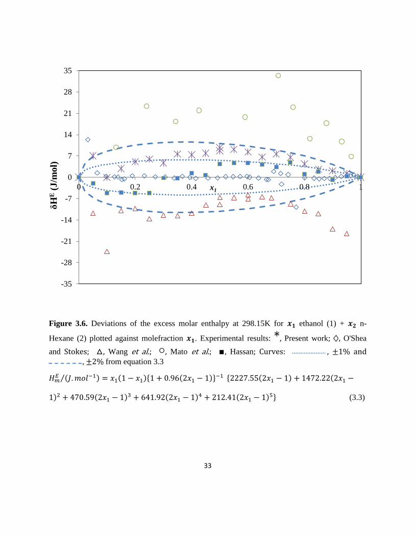
3.2.3 Verification of the calorimeter
The calorimeter verification step is essential because it ensures that the calorimeter is
reliable for making excess molar enthalpy measurements. Any experimentally measured will
have uncertainty which has the source, mainly from the calorimeter and the impurities of the
chemicals used for the study. In order to avoid any uncertainty caused by the calorimeter, the
calorimeter verification step is carried out. In this research work we measured the excess molar
enthalpy values of Ethanol (1) + n-Hexane (2) binary system at 298.15K and compared our
results with the other researchers who measured excess molar enthalpy of the same binary
system at same conditions. For this purpose we compared our results with O'Shea and Stokes,
(1986) who measured the heat of mixing of Ethanol + n-Hexane system and published the most
complete set of data and it is taken as main reference system. However the obtained result was
also compared with the data from Wang et al. (1992), Mato et al. (2006) and Hassan (2010).
33
Figure 3.6. Deviations of the excess molar enthalpy at 298.15K for ethanol (1) + n-
Hexane (2) plotted against molefraction . Experimental results: *, Present work; , O'Shea
and Stokes; , Wang et al.; , Mato et al.; ∎ Hassan; Curves: , ±1% and , ±2% from equation 3.3
𝑚𝑜𝑙 ⁄
(3.3)
-35
-28
-21
-14
-7
0
7
14
21
28
35
0 0.2 0.4 0.6 0.8 1
δH
E (
J/m
ol)
x1
34
The deviation of the experimental results from the smoothed results of O'Shea and Stokes are
plotted. The figure 3.6 shows that the average deviation of the present data is ±1.5% from the
enthalpy calculated using the O'Shea and Stokes correlation.
3.3 Calorimeter operational procedure
3.3.1 Binary system
Before the start of any calibration or mixing run, the water bath is maintained at 25.000 ±
0.005ᵒC for at least 24 hours. For a binary mixing run, the degassed component liquids are
pumped into the calorimeter mixing cell at specific flow rate by means of pump A and pump B.
The combined flow rate of the pumps gives a total displacement of 0.005 cm3/sec. By adjusting
the motor speed of the pumps, desired mole fraction of the mixtures can be achieved.
The mixing run for both binary and ternary mixtures are always started at equimolar
molefraction (i.e. ) and completed at and then the second half of the
measurements was started at and ended by measuring the enthalpy for the molefraction
. The excess molar enthalpy value for the molefraction was measured twice
just to make sure the repeatability of the experiment. The thermopile voltage for every individual
experimental point is the average value calculated from 100 data points recorded over a period of
time. The calibration and mixing run procedure is explained in detail in Appendix D
35
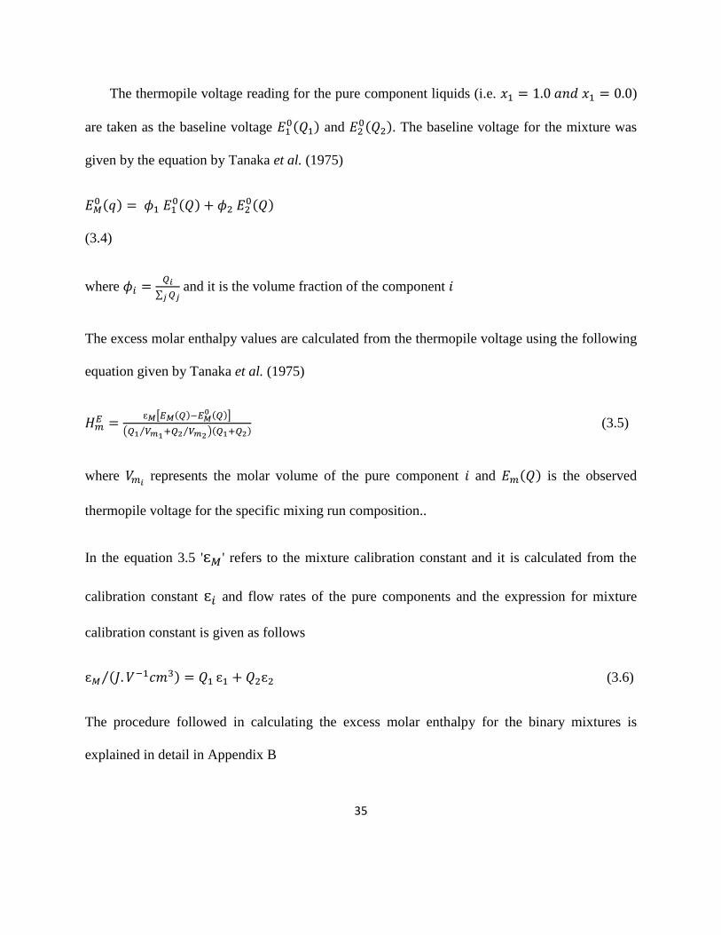
The thermopile voltage reading for the pure component liquids (i.e. 𝑛 )
are taken as the baseline voltage and
. The baseline voltage for the mixture was
given by the equation by Tanaka et al. (1975)
𝑞
(3.4)
where
∑ and it is the volume fraction of the component 𝑖
The excess molar enthalpy values are calculated from the thermopile voltage using the following
equation given by Tanaka et al. (1975)
ɛ [ ]
( ⁄
⁄ ) (3.5)
where represents the molar volume of the pure component 𝑖 and is the observed
thermopile voltage for the specific mixing run composition..
In the equation 3.5 'ɛ ' refers to the mixture calibration constant and it is calculated from the
calibration constant ɛ and flow rates of the pure components and the expression for mixture
calibration constant is given as follows
ɛ 𝑚 ⁄ ɛ ɛ (3.6)
The procedure followed in calculating the excess molar enthalpy for the binary mixtures is
explained in detail in Appendix B
36
3.3.2 Ternary system
Before measuring the ternary excess molar enthalpy, all three binary excess molar
enthalpy values involving the constituent species are measured first. i.e., component 1 +
(component 2 and 3), and component 2 + component 3 and the experimental values are fitted
with the Redlich-Kister polynomial equation. Three separate binary liquid mixtures with fixed
composition are prepared using component 2 and 3, such that the molefraction ratio of the
prepared mixtures are ⁄ ⁄ ⁄ ⁄ respectively, and these
mixtures are termed as pseudo-pure component. The excess molar enthalpy are
measured by mixing component 1 with the three pseudo-pure components separately, since the
resulting mixture from mixing component 1 + component (2+3) are not pure components, they
are called pseudo-binary mixtures. Measurement of is same as the measurement of
binary excess molar enthalpy, component 1 is taken in pump A and the pseudo-pure liquid is
taken in pump B and the procedure for the calculation of excess molar enthalpy is same as that of
binary system.
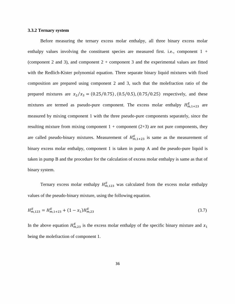
Ternary excess molar enthalpy was calculated from the excess molar enthalpy
values of the pseudo-binary mixture, using the following equation.
(3.7)
In the above equation is the excess molar enthalpy of the specific binary mixture and
being the molefraction of component 1.
37
Pseudo-Binary mixture preparation
Preparation of pseudo-pure component requires accurate weight measurements of pure
components. To make accurate weight measurements Mettler H315 precision balance was used
in this study, the balance has a 1000g weight range and 0.1mg precision range. For preparing the
mixture pure dewatered and degassed component 2 and 3 was taken. A pre-calculated amount of
component 2 was measured and taken in a flask, and then a pre-calculated amount of component
3 was measured and poured into the same flask. A magnetic bar is slipped into the flask and
placed on a magnetic stirrer and the liquid mixture is stirred for complete mixing of the
components.
Prior to mixture preparation, the temperature and humidity values of the room were noted
in order to do the weight correction due to buoyancy.
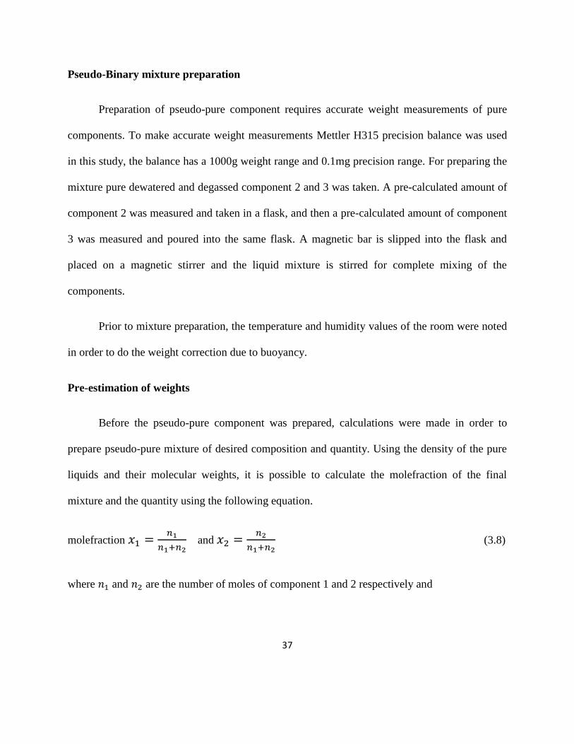
Pre-estimation of weights
Before the pseudo-pure component was prepared, calculations were made in order to
prepare pseudo-pure mixture of desired composition and quantity. Using the density of the pure
liquids and their molecular weights, it is possible to calculate the molefraction of the final
mixture and the quantity using the following equation.
molefraction
and
(3.8)
where 𝑛 and 𝑛 are the number of moles of component 1 and 2 respectively and
38
𝑛
(
) and 𝑛
(
) (3.9)
where 𝑚 and are the estimated mass and molecular weight of the component 𝑖, and the mass
of the compounds can be expressed as
𝑚 (3.10)
where and are the density and volume of the component 𝑖
Using the excel solver function, the mass of the component 1 and 2 was calculated for preparing
a mixture of specific composition.
Weight Correction
When weight measurements are carried out on any analytical balance, the object for
which the weight measured encounters the buoyancy effect of the surrounding air Bauer (1959).
Therefore the weight measurements should be adjusted for the buoyancy effect in order to avoid
error caused by the buoyancy effect of the air, Bauer (1959) explained a method for correcting
the weights measured in a fluid environment to vacuum condition. The molefraction and
molecular weight of the mixtures are calculated after correcting the weights to vacuum. The
details of the Bauer's method and a sample calculation are given in Appendix B2.
39
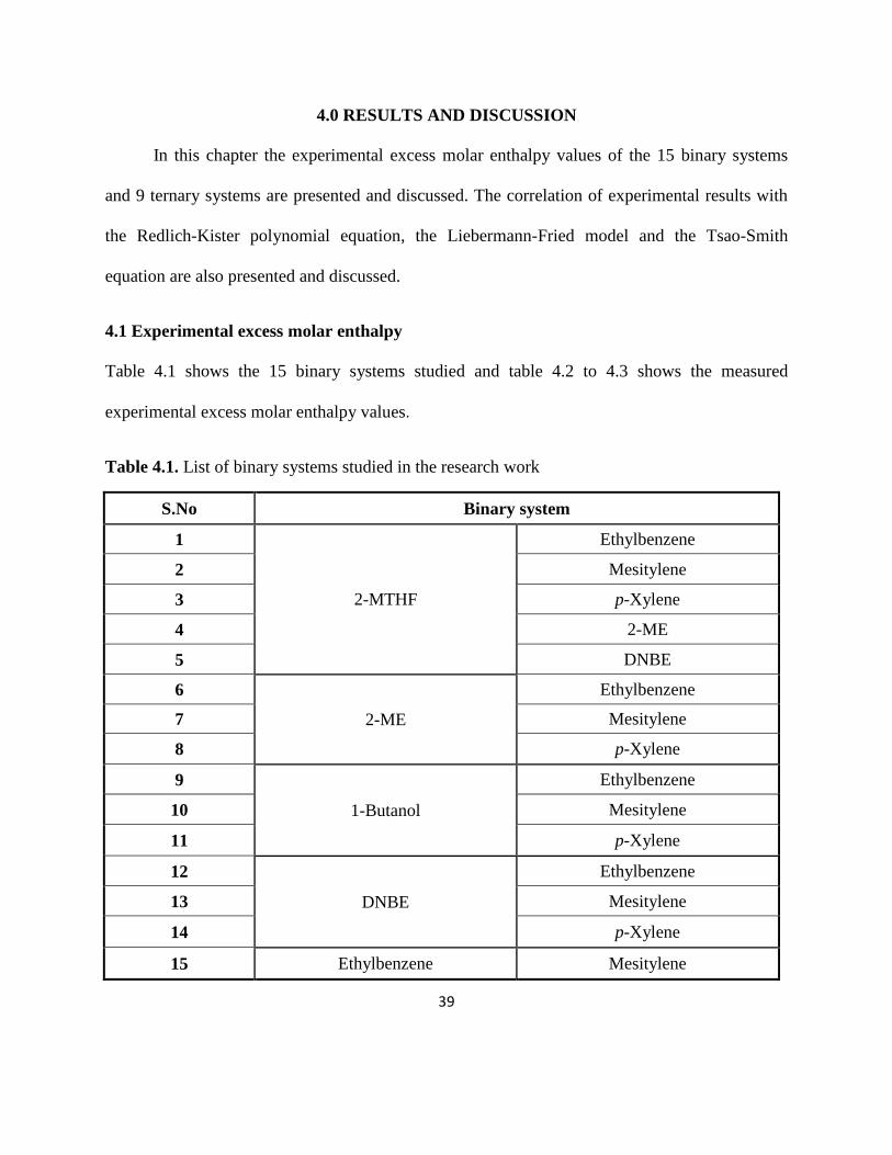
4.0 RESULTS AND DISCUSSION
In this chapter the experimental excess molar enthalpy values of the 15 binary systems
and 9 ternary systems are presented and discussed. The correlation of experimental results with
the Redlich-Kister polynomial equation, the Liebermann-Fried model and the Tsao-Smith
equation are also presented and discussed.
4.1 Experimental excess molar enthalpy
Table 4.1 shows the 15 binary systems studied and table 4.2 to 4.3 shows the measured
experimental excess molar enthalpy values.
Table 4.1. List of binary systems studied in the research work
S.No Binary system
1
2-MTHF
Ethylbenzene
2 Mesitylene
3 p-Xylene
4 2-ME
5 DNBE
6
2-ME
Ethylbenzene
7 Mesitylene
8 p-Xylene
9
1-Butanol
Ethylbenzene
10 Mesitylene
11 p-Xylene
12
DNBE
Ethylbenzene
13 Mesitylene
14 p-Xylene
15 Ethylbenzene Mesitylene
40
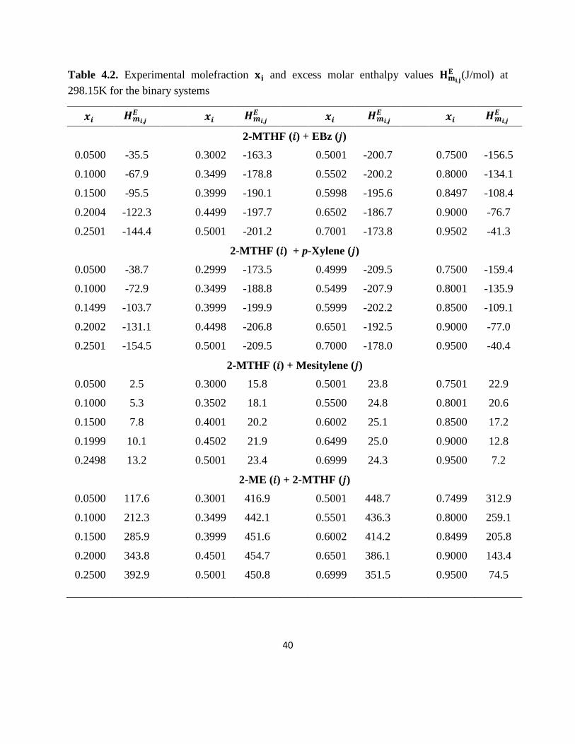
Table 4.2. Experimental molefraction and excess molar enthalpy values (J/mol) at
298.15K for the binary systems
2-MTHF (𝑖) + EBz (𝑗)
0.0500 -35.5
0.3002 -163.3
0.5001 -200.7
0.7500 -156.5
0.1000 -67.9
0.3499 -178.8
0.5502 -200.2
0.8000 -134.1
0.1500 -95.5
0.3999 -190.1
0.5998 -195.6
0.8497 -108.4
0.2004 -122.3
0.4499 -197.7
0.6502 -186.7
0.9000 -76.7
0.2501 -144.4
0.5001 -201.2
0.7001 -173.8
0.9502 -41.3
2-MTHF (𝑖) + p-Xylene (𝑗)
0.0500 -38.7
0.2999 -173.5
0.4999 -209.5
0.7500 -159.4
0.1000 -72.9
0.3499 -188.8
0.5499 -207.9
0.8001 -135.9
0.1499 -103.7
0.3999 -199.9
0.5999 -202.2
0.8500 -109.1
0.2002 -131.1
0.4498 -206.8
0.6501 -192.5
0.9000 -77.0
0.2501 -154.5
0.5001 -209.5
0.7000 -178.0
0.9500 -40.4
2-MTHF (𝑖) + Mesitylene (𝑗)
0.0500 2.5
0.3000 15.8
0.5001 23.8
0.7501 22.9
0.1000 5.3
0.3502 18.1
0.5500 24.8
0.8001 20.6
0.1500 7.8
0.4001 20.2
0.6002 25.1
0.8500 17.2
0.1999 10.1
0.4502 21.9
0.6499 25.0
0.9000 12.8
0.2498 13.2
0.5001 23.4
0.6999 24.3
0.9500 7.2
2-ME (𝑖) + 2-MTHF (𝑗)
0.0500 117.6
0.3001 416.9
0.5001 448.7
0.7499 312.9
0.1000 212.3
0.3499 442.1
0.5501 436.3
0.8000 259.1
0.1500 285.9
0.3999 451.6
0.6002 414.2
0.8499 205.8
0.2000 343.8
0.4501 454.7
0.6501 386.1
0.9000 143.4
0.2500 392.9
0.5001 450.8
0.6999 351.5
0.9500 74.5
41
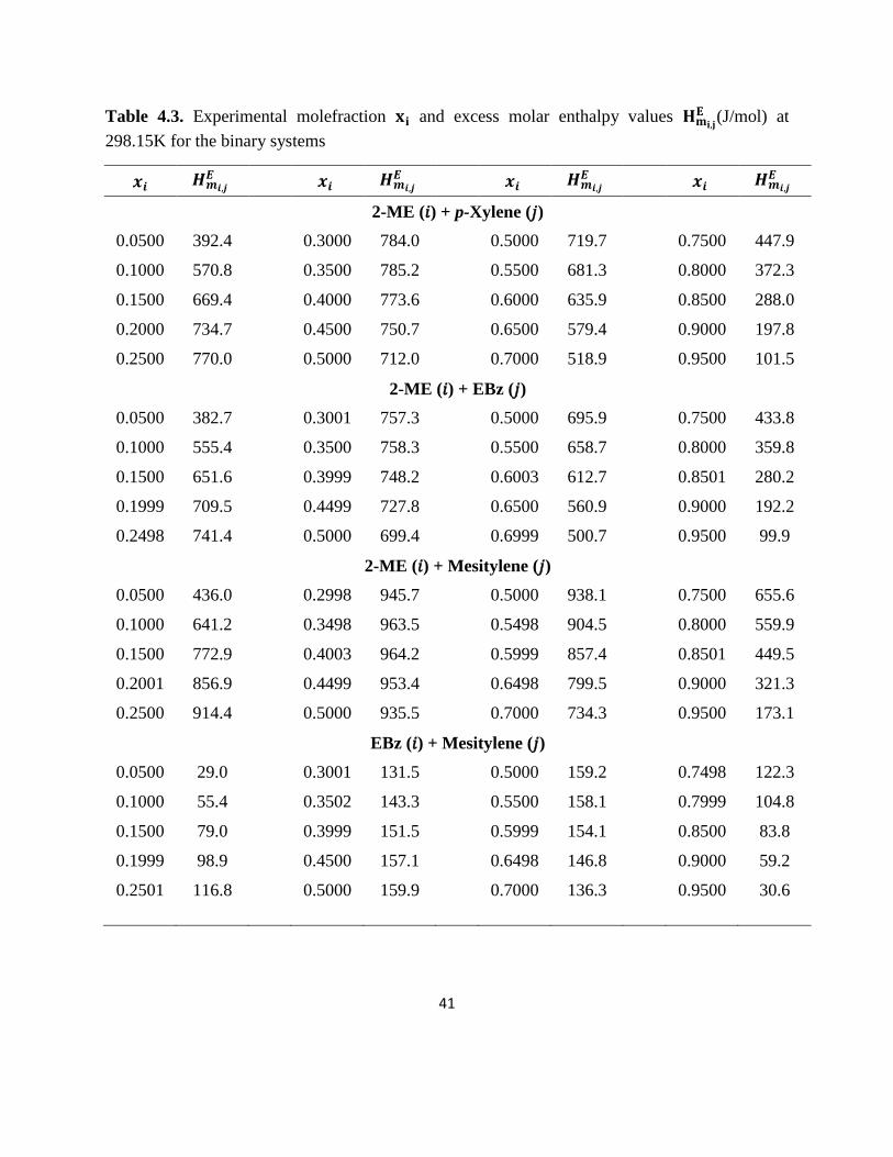
Table 4.3. Experimental molefraction and excess molar enthalpy values (J/mol) at
298.15K for the binary systems
2-ME (𝑖) + p-Xylene (𝑗)
0.0500 392.4
0.3000 784.0
0.5000 719.7
0.7500 447.9
0.1000 570.8
0.3500 785.2
0.5500 681.3
0.8000 372.3
0.1500 669.4
0.4000 773.6
0.6000 635.9
0.8500 288.0
0.2000 734.7
0.4500 750.7
0.6500 579.4
0.9000 197.8
0.2500 770.0
0.5000 712.0
0.7000 518.9
0.9500 101.5
2-ME (𝑖) + EBz (𝑗)
0.0500 382.7
0.3001 757.3
0.5000 695.9
0.7500 433.8
0.1000 555.4
0.3500 758.3
0.5500 658.7
0.8000 359.8
0.1500 651.6
0.3999 748.2
0.6003 612.7
0.8501 280.2
0.1999 709.5
0.4499 727.8
0.6500 560.9
0.9000 192.2
0.2498 741.4
0.5000 699.4
0.6999 500.7
0.9500 99.9
2-ME (𝑖) + Mesitylene (𝑗)
0.0500 436.0
0.2998 945.7
0.5000 938.1
0.7500 655.6
0.1000 641.2
0.3498 963.5
0.5498 904.5
0.8000 559.9
0.1500 772.9
0.4003 964.2
0.5999 857.4
0.8501 449.5
0.2001 856.9
0.4499 953.4
0.6498 799.5
0.9000 321.3
0.2500 914.4
0.5000 935.5
0.7000 734.3
0.9500 173.1
EBz (𝑖) + Mesitylene (𝑗)
0.0500 29.0
0.3001 131.5
0.5000 159.2
0.7498 122.3
0.1000 55.4
0.3502 143.3
0.5500 158.1
0.7999 104.8
0.1500 79.0
0.3999 151.5
0.5999 154.1
0.8500 83.8
0.1999 98.9
0.4500 157.1
0.6498 146.8
0.9000 59.2
0.2501 116.8
0.5000 159.9
0.7000 136.3
0.9500 30.6
42
Table 4.4. Experimental molefraction and excess molar enthalpy values (J/mol) at
298.15K for the binary systems
1-Butanol (𝑖) + p-Xylene (𝑗)
0.0500 538.3
0.3000 1012.2
0.5000 919.4
0.7500 518.5
0.1000 745.7
0.3500 1016.1
0.5500 860.3
0.8000 414.2
0.1500 866.4
0.4000 999.0
0.6000 789.3
0.8500 312.4
0.2000 940.8
0.4500 966.6
0.6500 704.9
0.9000 192.8
0.2500 989.3
0.5000 920.5
0.7000 616.2
0.9500 73.5
1-Butanol (𝑖) + Mesitylene (𝑗)
0.0500 554.8
0.3000 1073.1
0.5000 1004.5
0.7500 611.0
0.1000 773.8
0.3500 1082.3
0.5500 949.9
0.8000 503.0
0.1500 905.1
0.4000 1073.1
0.6000 882.0
0.8500 385.9
0.2000 987.2
0.4500 1047.4
0.6500 803.5
0.9000 246.1
0.2500 1041.7
0.5000 1007.8
0.7000 711.2
0.9500 101.6
1-Butanol (𝑖) + EBz (𝑗)
0.0500 547.6
0.3000 1052.1
0.5000 968.0
0.7500 558.8
0.1000 761.6
0.3500 1058.0
0.5500 908.3
0.8000 451.6
0.1500 889.3
0.4000 1045.7
0.6000 838.0
0.8500 339.9
0.2000 970.6
0.4500 1016.3
0.6500 755.7
0.9000 197.7
0.2500 1024.0
0.5000 969.3
0.7000 661.9
0.9500 78.9
DNBE (𝑖) + Mesitylene (𝑗)
0.0500 4.9
0.3000 26.1
0.5000 35.8
0.7500 30.3
0.1000 9.4
0.3500 29.2
0.5500 36.3
0.8000 26.4
0.1500 13.7
0.4000 32.2
0.6000 36.1
0.8500 21.5
0.2000 18.3
0.4500 34.3
0.6500 34.9
0.9000 15.2
0.2500 22.2
0.5000 35.5
0.7000 33.1
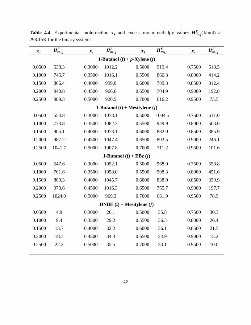
0.9500 10.0
43
Table 4.5. Experimental molefraction and excess molar enthalpy values (J/mol) at
298.15K for the binary systems
DNBE (𝑖) + p-Xylene (𝑗)
0.0500 -7.8
0.3000 -31.5
0.5000 -34.1
0.7500 -23.1
0.1000 -14.7
0.3500 -33.4
0.5500 -33.2
0.8000 -18.6
0.1500 -20.0
0.4000 -34.3
0.6000 -31.3
0.8500 -13.8
0.2000 -25.0
0.4500 -34.7
0.6500 -29.2
0.9000 -8.7
0.2500 -28.8
0.5000 -34.4
0.7000 -26.3
0.9500 -3.9
DNBE (𝑖) + 2-MTHF (𝑗)
0.0500 38.2
0.3000 155.4
0.5000 172.8
0.7500 120.2
0.1000 71.3
0.3500 165.8
0.5500 169.4
0.8000 99.5
0.1500 99.0
0.4000 171.8
0.6000 163.9
0.8500 75.2
0.2000 122.2
0.4500 174.7
0.6500 150.5
0.9000 48.9
0.2500 140.2
0.5000 174.3
0.7000 137.7
0.9500 20.9
DNBE (𝑖) + EBz (𝑗)
0.0500 23.1
0.3000 87.7
0.5000 92.9
0.7500 61.0
0.1000 42.2
0.3500 92.2
0.5500 89.5
0.8000 49.2
0.1500 58.2
0.4000 94.5
0.6000 84.8
0.8500 36.7
0.2000 71.0
0.4500 95.1
0.6500 77.4
0.9000 22.4
0.2500 80.8
0.5000 92.9
0.7000 69.6
0.9500 8.7
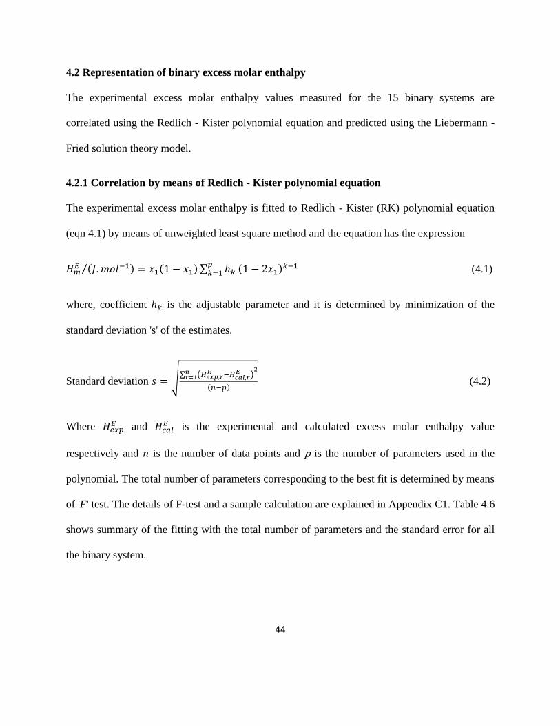
44
4.2 Representation of binary excess molar enthalpy
The experimental excess molar enthalpy values measured for the 15 binary systems are
correlated using the Redlich - Kister polynomial equation and predicted using the Liebermann -
Fried solution theory model.
4.2.1 Correlation by means of Redlich - Kister polynomial equation
The experimental excess molar enthalpy is fitted to Redlich - Kister (RK) polynomial equation
(eqn 4.1) by means of unweighted least square method and the equation has the expression
𝑚𝑜𝑙 ⁄ ∑
(4.1)
where, coefficient is the adjustable parameter and it is determined by minimization of the
standard deviation 's' of the estimates.
Standard deviation 𝑠 √∑ (
)
(4.2)
Where and
is the experimental and calculated excess molar enthalpy value
respectively and 𝑛 is the number of data points and p is the number of parameters used in the
polynomial. The total number of parameters corresponding to the best fit is determined by means
of 'F' test. The details of F-test and a sample calculation are explained in Appendix C1. Table 4.6
shows summary of the fitting with the total number of parameters and the standard error for all
the binary system.
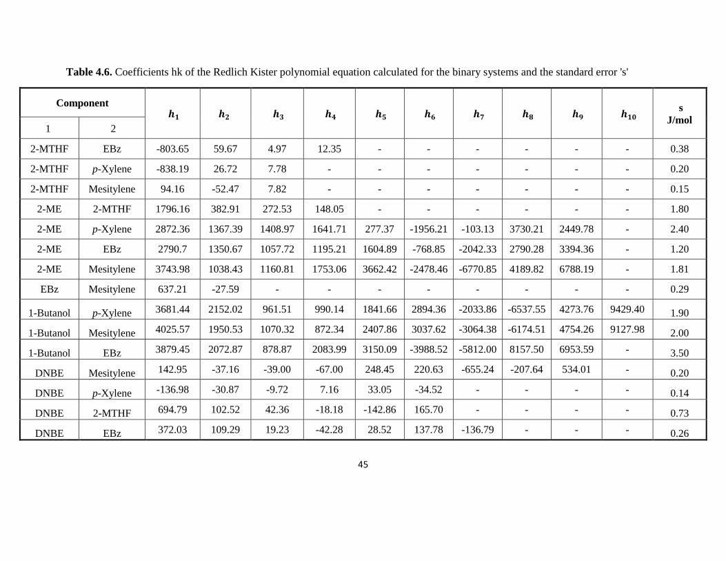
45
Table 4.6. Coefficients hk of the Redlich Kister polynomial equation calculated for the binary systems and the standard error 's'
Component
s
J/mol 1 2
2-MTHF EBz -803.65 59.67 4.97 12.35 - - - - - - 0.38
2-MTHF p-Xylene -838.19 26.72 7.78 - - - - - - - 0.20
2-MTHF Mesitylene 94.16 -52.47 7.82 - - - - - - - 0.15
2-ME 2-MTHF 1796.16 382.91 272.53 148.05 - - - - - - 1.80
2-ME p-Xylene 2872.36 1367.39 1408.97 1641.71 277.37 -1956.21 -103.13 3730.21 2449.78 - 2.40
2-ME EBz 2790.7 1350.67 1057.72 1195.21 1604.89 -768.85 -2042.33 2790.28 3394.36 - 1.20
2-ME Mesitylene 3743.98 1038.43 1160.81 1753.06 3662.42 -2478.46 -6770.85 4189.82 6788.19 - 1.81
EBz Mesitylene 637.21 -27.59 - - - - - - - - 0.29
1-Butanol p-Xylene 3681.44 2152.02 961.51 990.14 1841.66 2894.36 -2033.86 -6537.55 4273.76 9429.40 1.90
1-Butanol Mesitylene 4025.57 1950.53 1070.32 872.34 2407.86 3037.62 -3064.38 -6174.51 4754.26 9127.98 2.00
1-Butanol EBz 3879.45 2072.87 878.87 2083.99 3150.09 -3988.52 -5812.00 8157.50 6953.59 - 3.50
DNBE Mesitylene 142.95 -37.16 -39.00 -67.00 248.45 220.63 -655.24 -207.64 534.01 - 0.20
DNBE p-Xylene -136.98 -30.87 -9.72 7.16 33.05 -34.52 - - - - 0.14
DNBE 2-MTHF 694.79 102.52 42.36 -18.18 -142.86 165.70 - - - - 0.73
DNBE EBz 372.03 109.29 19.23 -42.28 28.52 137.78 -136.79 - - - 0.26
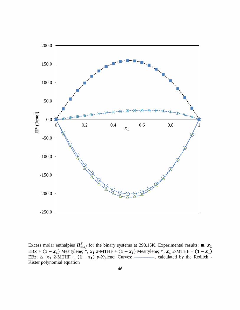
46
Excess molar enthalpies for the binary systems at 298.15K. Experimental results: ∎,
EBZ + Mesitylene; *, 2-MTHF + Mesitylene; , 2-MTHF + EBz; , 2-MTHF + p-Xylene: Curves: , calculated by the Redlich -
Kister polynomial equation
-250.0
-200.0
-150.0
-100.0
-50.0
0.0
50.0
100.0
150.0
200.0
0 0.2 0.4 0.6 0.8 1
HE (
J/m
ol)
𝑥1
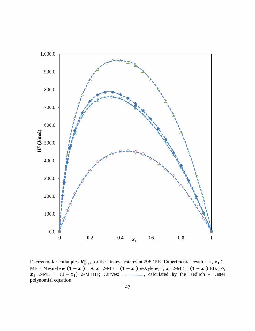
47
Excess molar enthalpies for the binary systems at 298.15K. Experimental results: , 2-
ME + Mesitylene ; ♦, 2-ME + p-Xylene; *, 2-ME + EBz; ,
2-ME + 2-MTHF; Curves: , calculated by the Redlich - Kister
polynomial equation
0.0
100.0
200.0
300.0
400.0
500.0
600.0
700.0
800.0
900.0
1,000.0
0 0.2 0.4 0.6 0.8 1
HE (
J/m
ol)
𝑥1
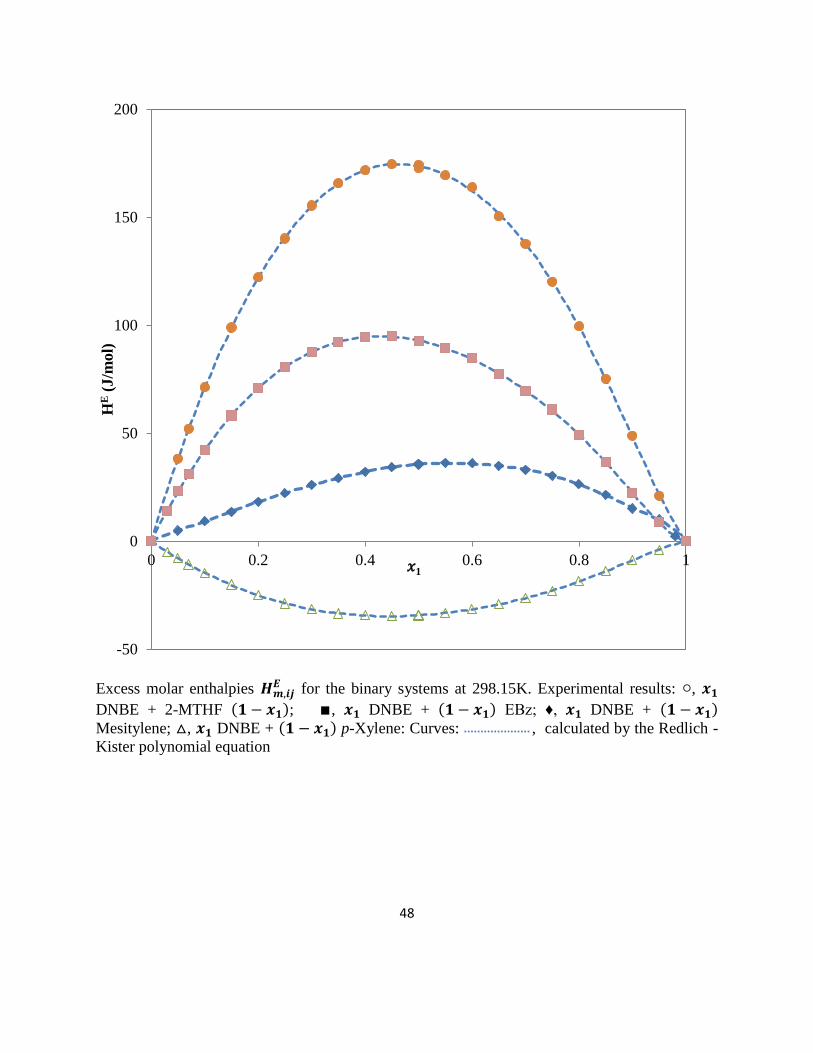
48
Excess molar enthalpies for the binary systems at 298.15K. Experimental results: ,
DNBE + 2-MTHF ; ∎, DNBE + EBz; ♦, DNBE +
Mesitylene; , DNBE + p-Xylene: Curves: , calculated by the Redlich -
Kister polynomial equation
-50
0
50
100
150
200
0 0.2 0.4 0.6 0.8 1
HE (
J/m
ol)
𝑥1
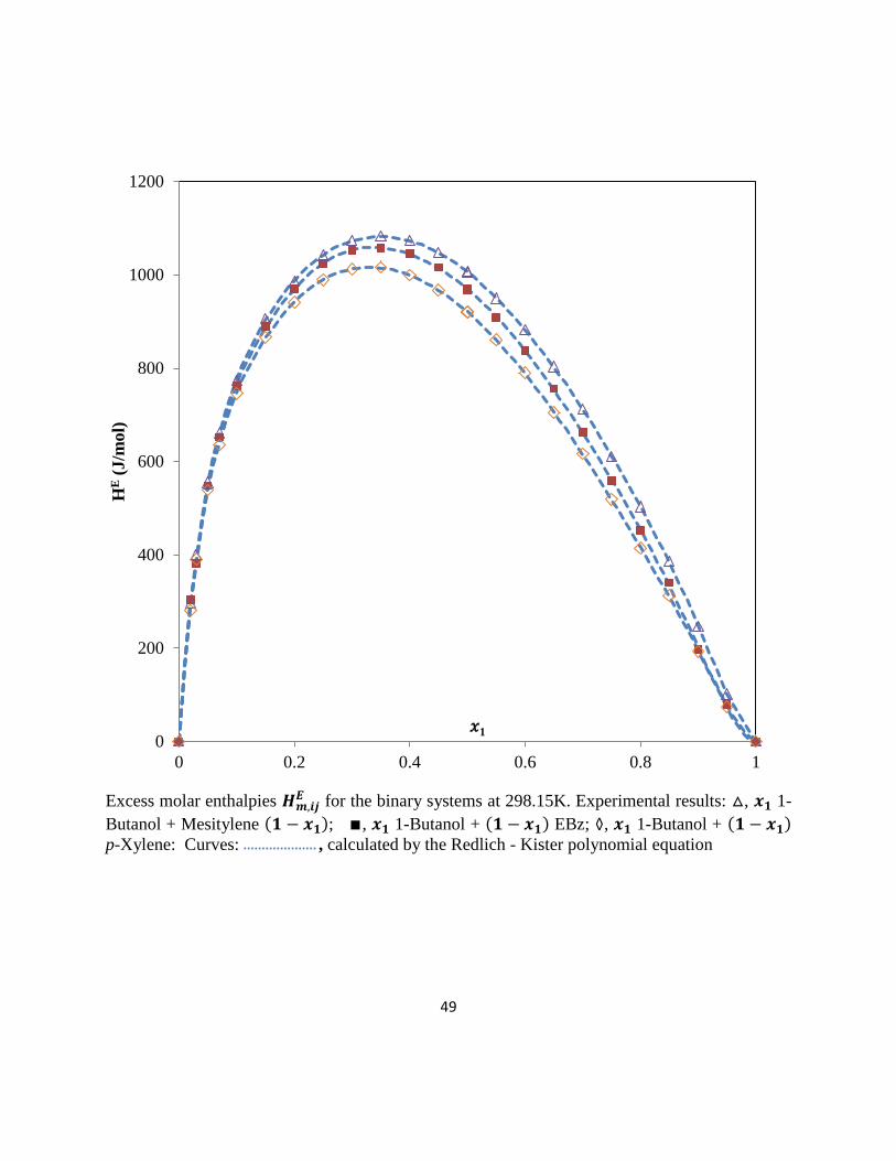
49
Excess molar enthalpies for the binary systems at 298.15K. Experimental results: , 1-
Butanol + Mesitylene ; ∎, 1-Butanol + EBz; ◊, 1-Butanol +
p-Xylene: Curves: , calculated by the Redlich - Kister polynomial equation
0
200
400
600
800
1000
1200
0 0.2 0.4 0.6 0.8 1
HE (
J/m
ol)
𝑥1
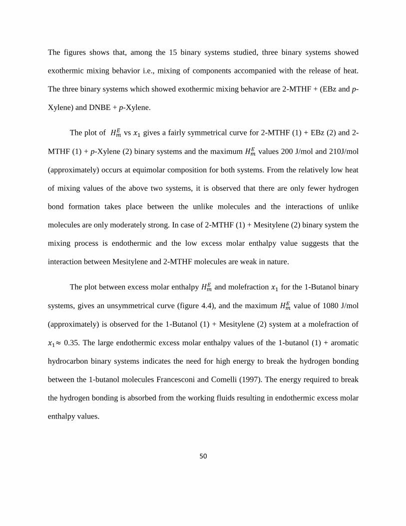
50
The figures shows that, among the 15 binary systems studied, three binary systems showed
exothermic mixing behavior i.e., mixing of components accompanied with the release of heat.
The three binary systems which showed exothermic mixing behavior are 2-MTHF + (EBz and p-
Xylene) and DNBE + p-Xylene.
The plot of vs gives a fairly symmetrical curve for 2-MTHF (1) + EBz (2) and 2-
MTHF (1) + p-Xylene (2) binary systems and the maximum values 200 J/mol and 210J/mol
(approximately) occurs at equimolar composition for both systems. From the relatively low heat
of mixing values of the above two systems, it is observed that there are only fewer hydrogen
bond formation takes place between the unlike molecules and the interactions of unlike
molecules are only moderately strong. In case of 2-MTHF (1) + Mesitylene (2) binary system the
mixing process is endothermic and the low excess molar enthalpy value suggests that the
interaction between Mesitylene and 2-MTHF molecules are weak in nature.
The plot between excess molar enthalpy and molefraction for the 1-Butanol binary
systems, gives an unsymmetrical curve (figure 4.4), and the maximum value of 1080 J/mol
(approximately) is observed for the 1-Butanol (1) + Mesitylene (2) system at a molefraction of
0.35. The large endothermic excess molar enthalpy values of the 1-butanol (1) + aromatic
hydrocarbon binary systems indicates the need for high energy to break the hydrogen bonding
between the 1-butanol molecules Francesconi and Comelli (1997). The energy required to break
the hydrogen bonding is absorbed from the working fluids resulting in endothermic excess molar
enthalpy values.
51
All the binary system involving 2-methoxyethanol have very high excess molar enthalpy
values with endothermic mixing behavior, with 2-ME (1) + Mesitylene (2) being the system with
highest value of 965.0 J/mol at 0.35. The high excess molar enthalpy values of the
2-methoxyethanol binary system can be attributed to the fact that high energy is needed to break
the strong intermolecular bond between the - OH and -OCH3 molecules Kinart et al. (2002).
The DNBE binary systems exhibits a different mixing pattern, it mixes endothermically
with 2-MTHF, EBz and Mesitylene with relatively low excess molar enthalpy values, but it
shows an exothermic mixing behavior with p-Xylene with very low excess molar enthalpy
values. For the DNBE (1) + 2-MTHF (2) system, the maximum values of excess molar enthalpy
is 174.7 J/mol at a molefraction of 0.40 and 95.1 J/mol for DNBE (1) + EBz (2) at a
molefraction of 0.45. For the other binary systems of DNBE the maximum values of excess
molar enthalpies are significantly low. The EBz (1) and Mesitylene (2) mixing process is
endothermic and the maximum excess molar enthalpy value is 160 J/mol and measured at
equimolar composition.
4.2.2 Correlation by means of Liebermann-Fried model
Liebermann-Fried model has notable success in predicting the excess property values of
mixtures. The method uses the pure component properties such as molar volume and isobaric
thermal expansivity to calculate the binary interaction parameters through regression of excess
molar enthalpy data, and these interaction parameters are used to predict the multicomponent
excess molar enthalpy values. Peng et al. (2001) described the thermodynamic relation using the
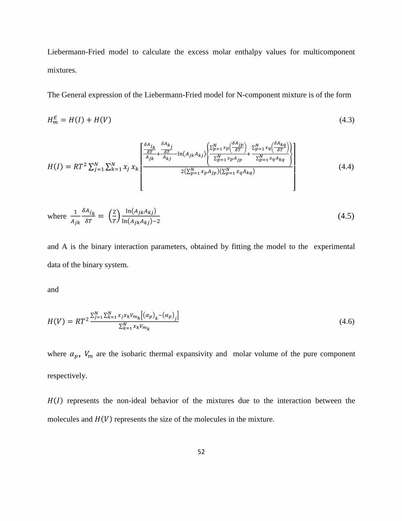
52
Liebermann-Fried model to calculate the excess molar enthalpy values for multicomponent
mixtures.
The General expression of the Liebermann-Fried model for N-component mixture is of the form
(4.3)
∑ ∑
[
( )∑ (
)
∑
∑ (
)
∑
(∑ )(∑
)
]
(4.4)
where
(
)
( )
( ) (4.5)
and A is the binary interaction parameters, obtained by fitting the model to the experimental
data of the binary system.
and
∑ ∑
*( ) ( )
+
∑
(4.6)
where , are the isobaric thermal expansivity and molar volume of the pure component
respectively.
represents the non-ideal behavior of the mixtures due to the interaction between the
molecules and represents the size of the molecules in the mixture.
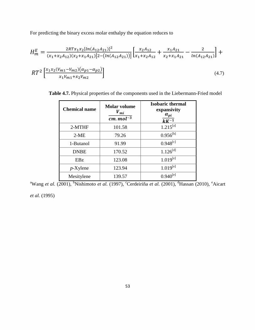
53
For predicting the binary excess molar enthalpy the equation reduces to
[ ]
[ ( )]*
+
* ( )
+ (4.7)
Table 4.7. Physical properties of the components used in the Liebermann-Fried model
Chemical name
Molar volume
Isobaric thermal
expansivity
2-MTHF 101.58 1.215[a]
2-ME 79.26 0.956[b]
1-Butanol 91.99 0.948[c]
DNBE 170.52 1.126[d]
EBz 123.08 1.019[e]
p-Xylene 123.94 1.019[e]
Mesitylene 139.57 0.940[e]
aWang et al. (2001),
bNishimoto et al. (1997),
cCerdeiriña et al. (2001),
dHassan (2010),
eAicart
et al. (1995)
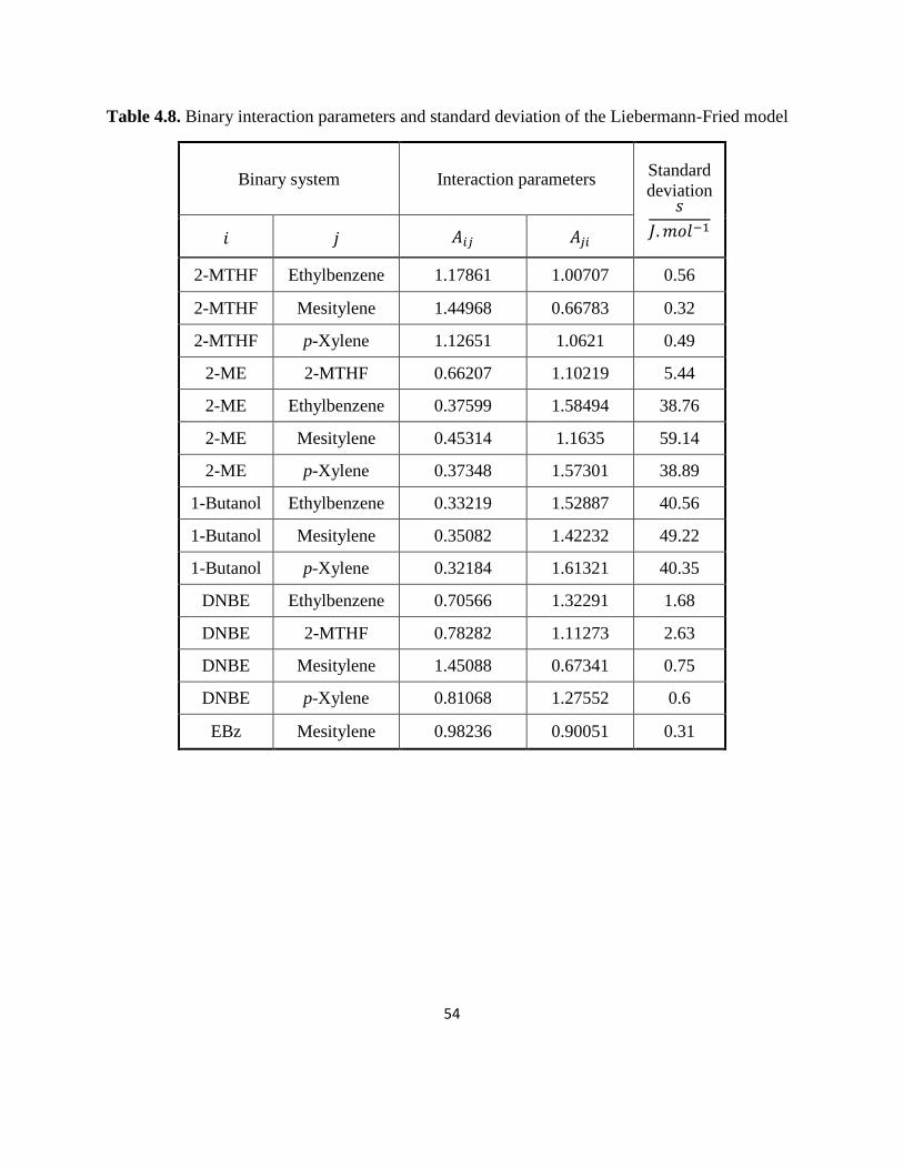
54
Table 4.8. Binary interaction parameters and standard deviation of the Liebermann-Fried model
Binary system Interaction parameters Standard
deviation 𝑠
𝑚𝑜𝑙
𝑖 𝑗
2-MTHF Ethylbenzene 1.17861 1.00707 0.56
2-MTHF Mesitylene 1.44968 0.66783 0.32
2-MTHF p-Xylene 1.12651 1.0621 0.49
2-ME 2-MTHF 0.66207 1.10219 5.44
2-ME Ethylbenzene 0.37599 1.58494 38.76
2-ME Mesitylene 0.45314 1.1635 59.14
2-ME p-Xylene 0.37348 1.57301 38.89
1-Butanol Ethylbenzene 0.33219 1.52887 40.56
1-Butanol Mesitylene 0.35082 1.42232 49.22
1-Butanol p-Xylene 0.32184 1.61321 40.35
DNBE Ethylbenzene 0.70566 1.32291 1.68
DNBE 2-MTHF 0.78282 1.11273 2.63
DNBE Mesitylene 1.45088 0.67341 0.75
DNBE p-Xylene 0.81068 1.27552 0.6
EBz Mesitylene 0.98236 0.90051 0.31
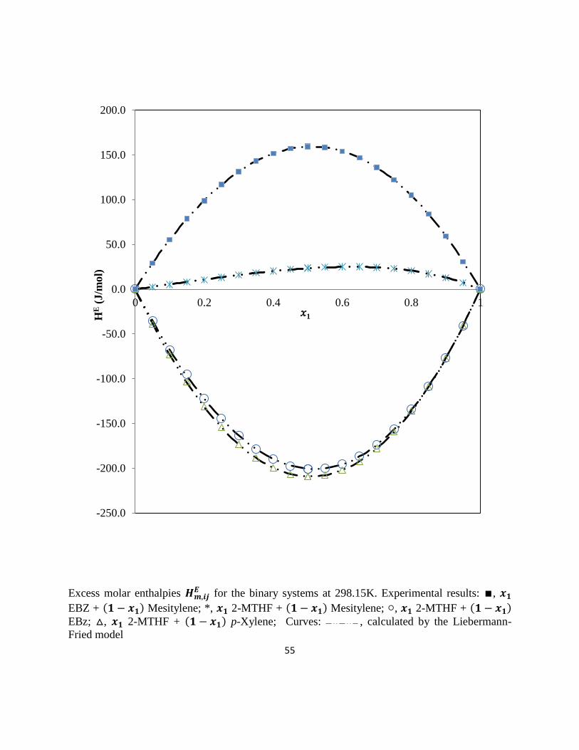
55
Excess molar enthalpies for the binary systems at 298.15K. Experimental results: ∎,
EBZ + Mesitylene; *, 2-MTHF + Mesitylene; , 2-MTHF + EBz; , 2-MTHF + p-Xylene; Curves: , calculated by the Liebermann-
Fried model
-250.0
-200.0
-150.0
-100.0
-50.0
0.0
50.0
100.0
150.0
200.0
0 0.2 0.4 0.6 0.8 1
HE (
J/m
ol)
𝑥1
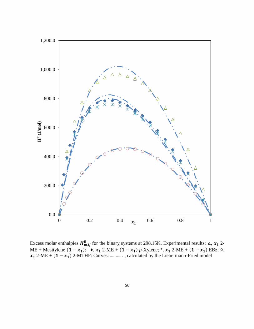
56
Excess molar enthalpies for the binary systems at 298.15K. Experimental results: , 2-
ME + Mesitylene ; ♦, 2-ME + p-Xylene; *, 2-ME + EBz; ,
2-ME + 2-MTHF: Curves: , calculated by the Liebermann-Fried model
0.0
200.0
400.0
600.0
800.0
1,000.0
1,200.0
0 0.2 0.4 0.6 0.8 1
HE (
J/m
ol)
𝑥1
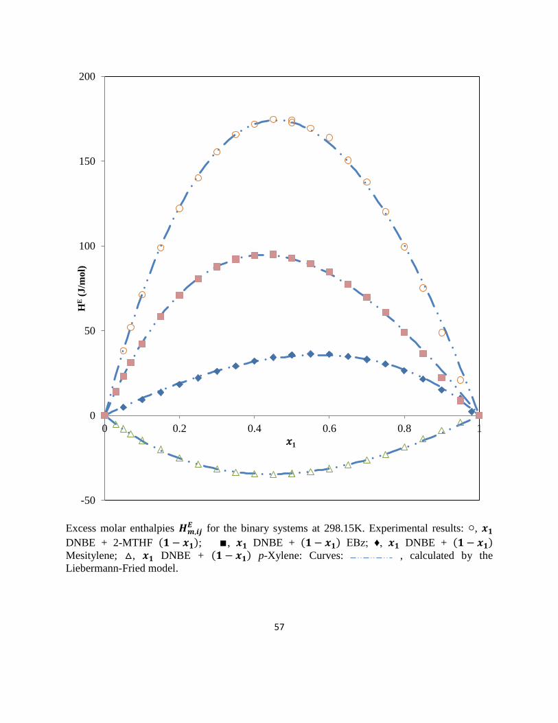
57
Excess molar enthalpies for the binary systems at 298.15K. Experimental results: ,
DNBE + 2-MTHF ; ∎, DNBE + EBz; ♦, DNBE +
Mesitylene; , DNBE + p-Xylene: Curves: , calculated by the
Liebermann-Fried model.
-50
0
50
100
150
200
0 0.2 0.4 0.6 0.8 1
HE (
J/m
ol)
𝑥1
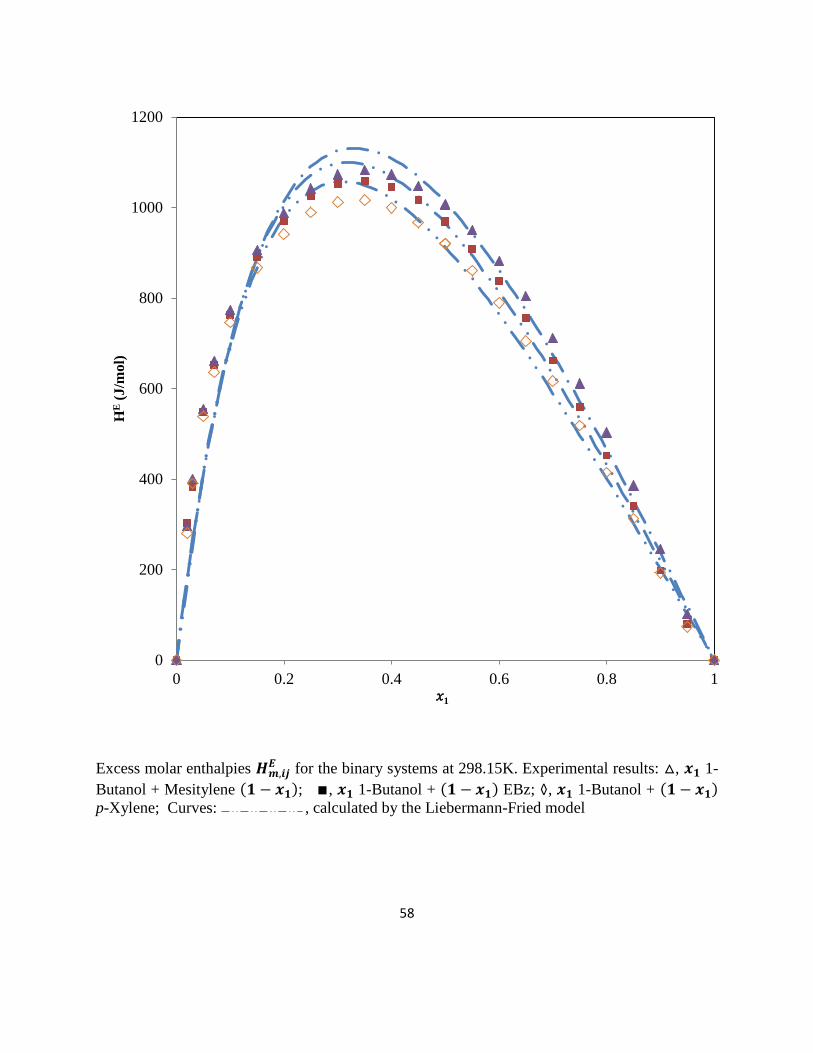
58
Excess molar enthalpies for the binary systems at 298.15K. Experimental results: , 1-
Butanol + Mesitylene ; ∎, 1-Butanol + EBz; ◊, 1-Butanol +
p-Xylene; Curves: , calculated by the Liebermann-Fried model
0
200
400
600
800
1000
1200
0 0.2 0.4 0.6 0.8 1
HE (
J/m
ol)
𝑥1
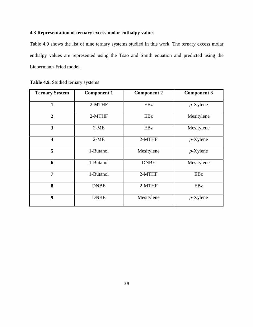
59
4.3 Representation of ternary excess molar enthalpy values
Table 4.9 shows the list of nine ternary systems studied in this work. The ternary excess molar
enthalpy values are represented using the Tsao and Smith equation and predicted using the
Liebermann-Fried model.
Table 4.9. Studied ternary systems
Ternary System Component 1 Component 2 Component 3
1 2-MTHF EBz p-Xylene
2 2-MTHF EBz Mesitylene
3 2-ME EBz Mesitylene
4 2-ME 2-MTHF p-Xylene
5 1-Butanol Mesitylene p-Xylene
6 1-Butanol DNBE Mesitylene
7 1-Butanol 2-MTHF EBz
8 DNBE 2-MTHF EBz
9 DNBE Mesitylene p-Xylene
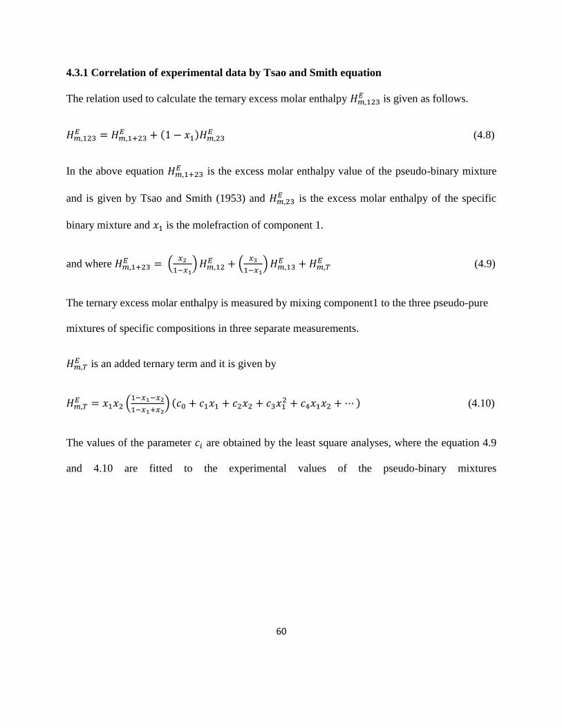
60
4.3.1 Correlation of experimental data by Tsao and Smith equation
The relation used to calculate the ternary excess molar enthalpy is given as follows.
(4.8)
In the above equation is the excess molar enthalpy value of the pseudo-binary mixture
and is given by Tsao and Smith (1953) and is the excess molar enthalpy of the specific
binary mixture and is the molefraction of component 1.
and where (
)
(
)
(4.9)
The ternary excess molar enthalpy is measured by mixing component1 to the three pseudo-pure
mixtures of specific compositions in three separate measurements.
is an added ternary term and it is given by
(
)
(4.10)
The values of the parameter are obtained by the least square analyses, where the equation 4.9
and 4.10 are fitted to the experimental values of the pseudo-binary mixtures
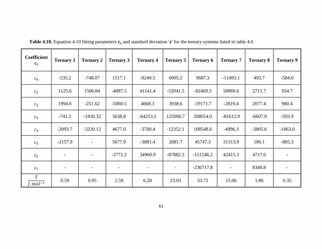
61
Table 4.10. Equation 4.10 fitting parameters and standard deviation ' ' for the ternary systems listed in table 4.6
Coefficient
Ternary 1 Ternary 2 Ternary 3 Ternary 4 Ternary 5 Ternary 6 Ternary 7 Ternary 8 Ternary 9
-535.2 -748.07 1517.1 -9249.5 6005.2 9687.3 -11493.1 493.7 -584.0
1125.6 1506.84 -4987.5 41141.4 -52041.5 -82469.3 50869.6 2711.7 934.7
1994.6 -251.62 -5060.5 4668.3 3938.6 -19171.7 -2819.4 2077.4 980.4
-741.1 -1830.32 5638.8 -64253.1 125006.7 208054.0 -81612.9 -6607.0 -593.9
-2093.7 -3220.12 4677.0 -3700.4 -12352.1 108548.6 -4996.3 -3805.6 -1063.0
-2157.9 - 5677.9 -3881.4 2681.7 45747.3 31313.9 186.1 -885.3
- - -2772.2 34960.9 -87882.3 -151146.2 42415.3 4717.0 -
- - - - - -236717.8 - 8340.8 -
𝑚𝑜𝑙 0.59 0.95 2.59 6.20 23.03 33.72 15.06 1.86 0.35
62
Table 4.10 summarizes the values of the coefficient for the nine ternary systems, while fitting
the experimental excess molar enthalpy data to the ternary system, the binary contribution term
is calculated by means of Redlich-Kister equation with values of the coefficients given in
the table 4.6. The ternary excess molar enthalpy value and the excess molar enthalpy
values of the pseudo-binary mixtures are reported in the table 4.11 to table 4.19 for the nine
ternary systems. The ternary excess molar enthalpy values are then plotted in the Roozeboom
diagram and it shows that there is no indication of an local maxima for all of the systems and the
maximum value of for all the ternary system are located at the edge of the plot for the
constituent binary systems.
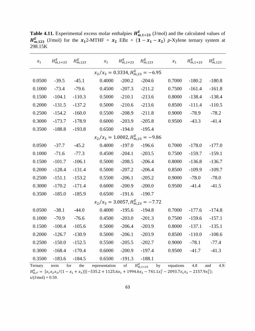
63
Table 4.11. Experimental excess molar enthalpies (J/mol) and the calculated values of
(J/mol) for the 2-MTHF + EBz + p-Xylene ternary system at
298.15K
⁄
0.0500 -39.5 -45.1
0.4000 -200.2 -204.6
0.7000 -180.2 -180.8
0.1000 -73.4 -79.6
0.4500 -207.3 -211.2
0.7500 -161.4 -161.8
0.1500 -104.1 -110.3
0.5000 -210.1 -213.6
0.8000 -138.4 -138.4
0.2000 -131.5 -137.2
0.5000 -210.6 -213.6
0.8500 -111.4 -110.5
0.2500 -154.2 -160.0
0.5500 -208.9 -211.8
0.9000 -78.9 -78.2
0.3000 -173.7 -178.9
0.6000 -203.9 -205.8
0.9500 -43.3 -41.4
0.3500 -188.8 -193.8
0.6500 -194.0 -195.4
⁄
0.0500 -37.7 -45.2
0.4000 -197.0 -196.6
0.7000 -178.0 -177.0
0.1000 -71.6 -77.3
0.4500 -204.1 -203.5
0.7500 -159.7 -159.1
0.1500 -101.7 -106.1
0.5000 -208.5 -206.4
0.8000 -136.8 -136.7
0.2000 -128.4 -131.4
0.5000 -207.2 -206.4
0.8500 -109.9 -109.7
0.2500 -151.1 -153.2
0.5500 -206.1 -205.2
0.9000 -78.0 -78.0
0.3000 -170.2 -171.4
0.6000 -200.9 -200.0
0.9500 -41.4 -41.5
0.3500 -185.0 -185.9
0.6500 -191.6 -190.7
⁄
0.0500 -38.1 -44.0
0.4000 -195.6 -194.8
0.7000 -177.6 -174.8
0.1000 -70.9 -76.6
0.4500 -203.0 -201.3
0.7500 -159.6 -157.1
0.1500 -100.4 -105.6
0.5000 -206.4 -203.9
0.8000 -137.1 -135.1
0.2000 -126.7 -130.9
0.5000 -206.1 -203.9
0.8500 -110.0 -108.6
0.2500 -150.0 -152.5
0.5500 -205.5 -202.7
0.9000 -78.1 -77.4
0.3000 -168.4 -170.4
0.6000 -200.9 -197.4
0.9500 -41.7 -41.3
0.3500 -183.6 -184.5 0.6500 -191.3 -188.1
Ternary term for the representation of by equations 4.8 and 4.9:
[ ⁄ ]
;
s/(J/mol) = 0.59.
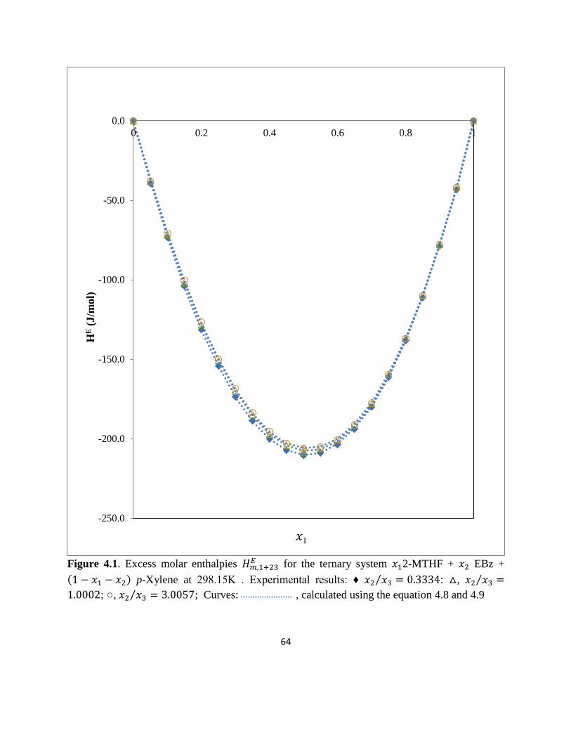
64
Figure 4.1. Excess molar enthalpies for the ternary system 2-MTHF + EBz +
p-Xylene at 298.15K . Experimental results: ♦ ⁄ : , ⁄
; , ⁄ ; Curves: , calculated using the equation 4.8 and 4.9
-250.0
-200.0
-150.0
-100.0
-50.0
0.0
0 0.2 0.4 0.6 0.8 1
HE (
J/m
ol)
𝑥1
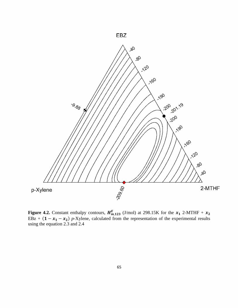
65
Figure 4.2. Constant enthalpy contours, (J/mol) at 298.15K for the 2-MTHF +
EBz + p-Xylene, calculated from the representation of the experimental results
using the equation 2.3 and 2.4
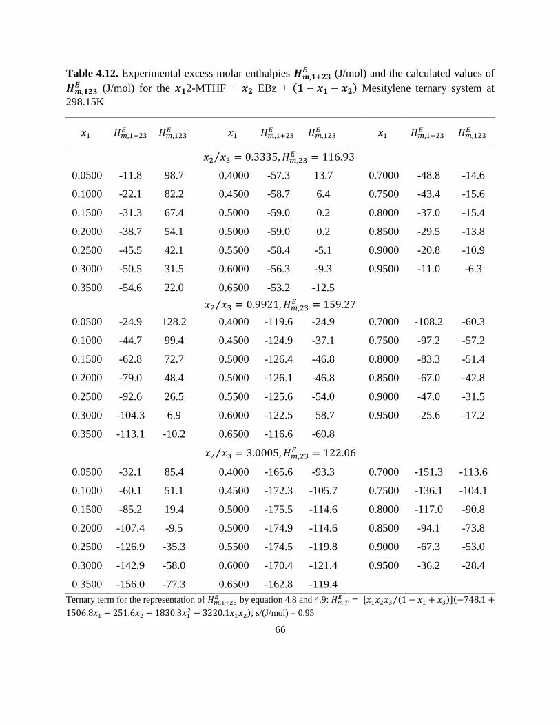
66
Table 4.12. Experimental excess molar enthalpies (J/mol) and the calculated values of
(J/mol) for the 2-MTHF + EBz + Mesitylene ternary system at
298.15K
⁄
0.0500 -11.8 98.7
0.4000 -57.3 13.7
0.7000 -48.8 -14.6
0.1000 -22.1 82.2
0.4500 -58.7 6.4
0.7500 -43.4 -15.6
0.1500 -31.3 67.4
0.5000 -59.0 0.2
0.8000 -37.0 -15.4
0.2000 -38.7 54.1
0.5000 -59.0 0.2
0.8500 -29.5 -13.8
0.2500 -45.5 42.1
0.5500 -58.4 -5.1
0.9000 -20.8 -10.9
0.3000 -50.5 31.5
0.6000 -56.3 -9.3
0.9500 -11.0 -6.3
0.3500 -54.6 22.0
0.6500 -53.2 -12.5
⁄
0.0500 -24.9 128.2
0.4000 -119.6 -24.9
0.7000 -108.2 -60.3
0.1000 -44.7 99.4
0.4500 -124.9 -37.1
0.7500 -97.2 -57.2
0.1500 -62.8 72.7
0.5000 -126.4 -46.8
0.8000 -83.3 -51.4
0.2000 -79.0 48.4
0.5000 -126.1 -46.8
0.8500 -67.0 -42.8
0.2500 -92.6 26.5
0.5500 -125.6 -54.0
0.9000 -47.0 -31.5
0.3000 -104.3 6.9
0.6000 -122.5 -58.7
0.9500 -25.6 -17.2
0.3500 -113.1 -10.2
0.6500 -116.6 -60.8
⁄
0.0500 -32.1 85.4
0.4000 -165.6 -93.3
0.7000 -151.3 -113.6
0.1000 -60.1 51.1
0.4500 -172.3 -105.7
0.7500 -136.1 -104.1
0.1500 -85.2 19.4
0.5000 -175.5 -114.6
0.8000 -117.0 -90.8
0.2000 -107.4 -9.5
0.5000 -174.9 -114.6
0.8500 -94.1 -73.8
0.2500 -126.9 -35.3
0.5500 -174.5 -119.8
0.9000 -67.3 -53.0
0.3000 -142.9 -58.0
0.6000 -170.4 -121.4
0.9500 -36.2 -28.4
0.3500 -156.0 -77.3 0.6500 -162.8 -119.4
Ternary term for the representation of by equation 4.8 and 4.9:
[ ⁄ ]
; s/(J/mol) = 0.95
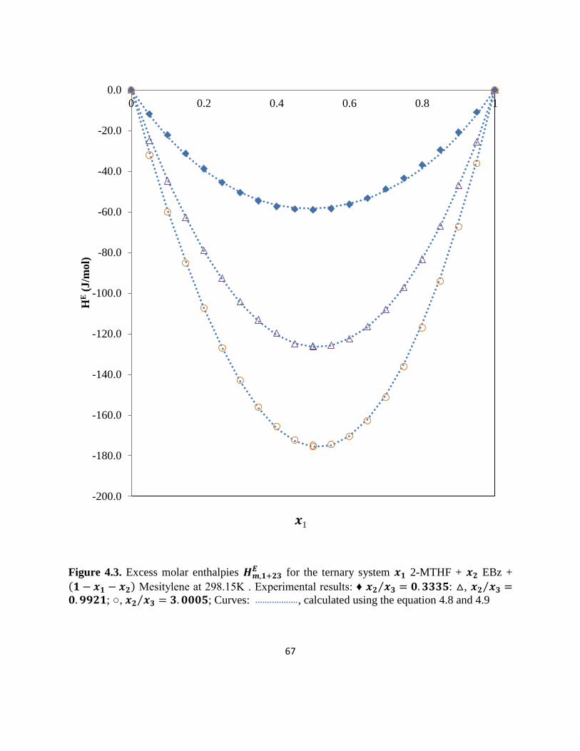
67
Figure 4.3. Excess molar enthalpies for the ternary system 2-MTHF + EBz +
Mesitylene at 298.15K . Experimental results: ♦ ⁄ : , ⁄ ; , ⁄ ; Curves: , calculated using the equation 4.8 and 4.9
-200.0
-180.0
-160.0
-140.0
-120.0
-100.0
-80.0
-60.0
-40.0
-20.0
0.0
0 0.2 0.4 0.6 0.8 1
HE (
J/m
ol)
𝒙1
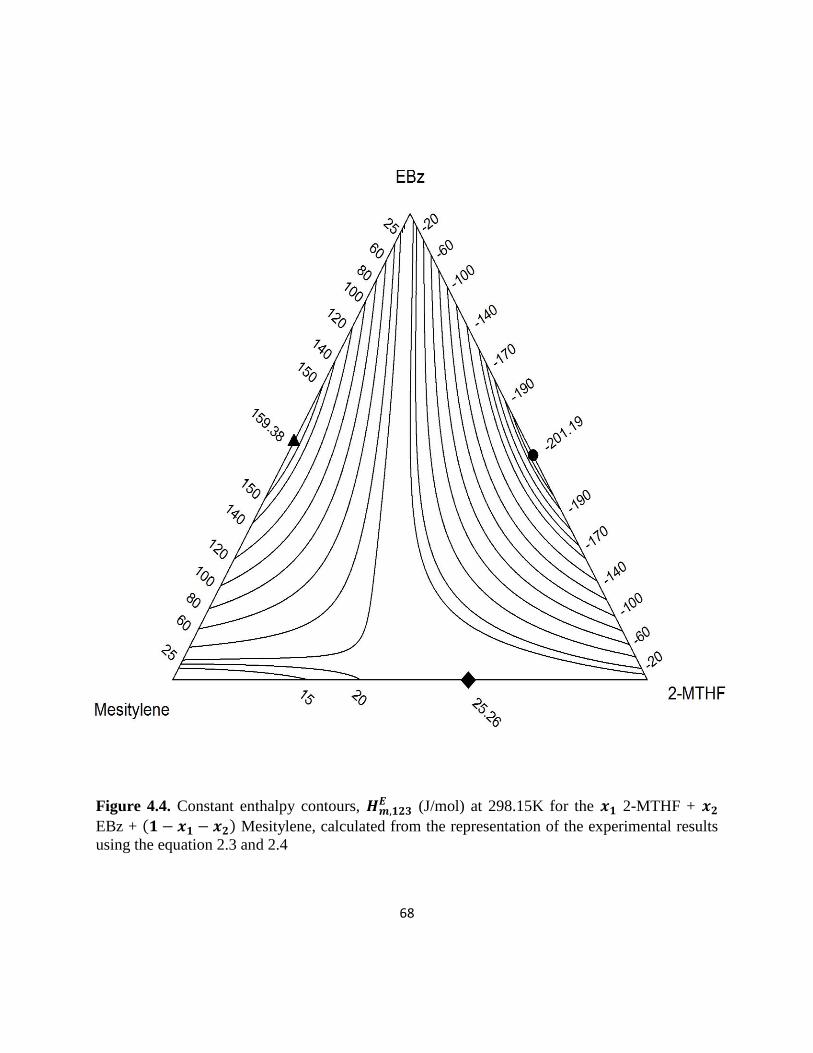
68
Figure 4.4. Constant enthalpy contours, (J/mol) at 298.15K for the 2-MTHF +
EBz + Mesitylene, calculated from the representation of the experimental results
using the equation 2.3 and 2.4
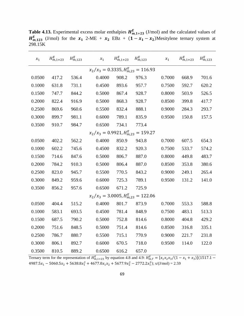
69
Table 4.13. Experimental excess molar enthalpies (J/mol) and the calculated values of
(J/mol) for the 2-ME + EBz + Mesitylene ternary system at
298.15K
⁄
0.0500 417.2 536.4
0.4000 908.2 976.3
0.7000 668.9 701.6
0.1000 631.8 731.1
0.4500 893.6 957.7
0.7500 592.7 620.2
0.1500 747.7 844.2
0.5000 867.4 928.7
0.8000 503.9 526.5
0.2000 822.4 916.9
0.5000 868.3 928.7
0.8500 399.8 417.7
0.2500 869.6 960.6
0.5500 832.4 888.1
0.9000 284.3 293.7
0.3000 899.7 981.1
0.6000 789.1 835.9
0.9500 150.8 157.5
0.3500 910.7 984.7
0.6500 734.1 773.4
⁄
0.0500 402.2 562.2
0.4000 850.9 943.8
0.7000 607.5 654.3
0.1000 602.2 745.6
0.4500 832.2 920.3
0.7500 533.7 574.2
0.1500 714.6 847.6
0.5000 806.7 887.0
0.8000 449.8 483.7
0.2000 784.2 910.3
0.5000 806.4 887.0
0.8500 353.8 380.6
0.2500 823.0 945.7
0.5500 770.5 843.2
0.9000 249.1 265.4
0.3000 849.2 959.6
0.6000 725.3 789.1
0.9500 131.2 141.0
0.3500 856.2 957.6
0.6500 671.2 725.9
⁄
0.0500 404.4 515.2
0.4000 801.7 873.9
0.7000 553.3 588.8
0.1000 583.1 693.5
0.4500 781.4 848.9
0.7500 483.1 513.3
0.1500 687.5 790.2
0.5000 752.8 814.6
0.8000 404.8 429.2
0.2000 751.6 848.5
0.5000 751.4 814.6
0.8500 316.8 335.1
0.2500 786.7 880.7
0.5500 715.1 770.9
0.9000 221.7 231.8
0.3000 806.1 892.7
0.6000 670.5 718.0
0.9500 114.0 122.0
0.3500 810.5 889.2 0.6500 616.2 657.0
Ternary term for the representation of by equation 4.8 and 4.9:
[ ⁄ ]
; s/(J/mol) = 2.59
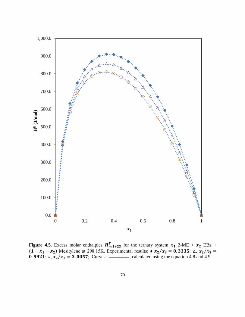
70
Figure 4.5. Excess molar enthalpies for the ternary system 2-ME + EBz +
Mesitylene at 298.15K. Experimental results: ♦ ⁄ : , ⁄ ; , ⁄ ; Curves: , calculated using the equation 4.8 and 4.9
0.0
100.0
200.0
300.0
400.0
500.0
600.0
700.0
800.0
900.0
1,000.0
0 0.2 0.4 0.6 0.8 1
HE (
J/m
ol)
𝒙1
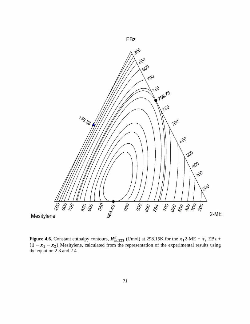
71
Figure 4.6. Constant enthalpy contours, (J/mol) at 298.15K for the 2-ME + EBz +
Mesitylene, calculated from the representation of the experimental results using
the equation 2.3 and 2.4
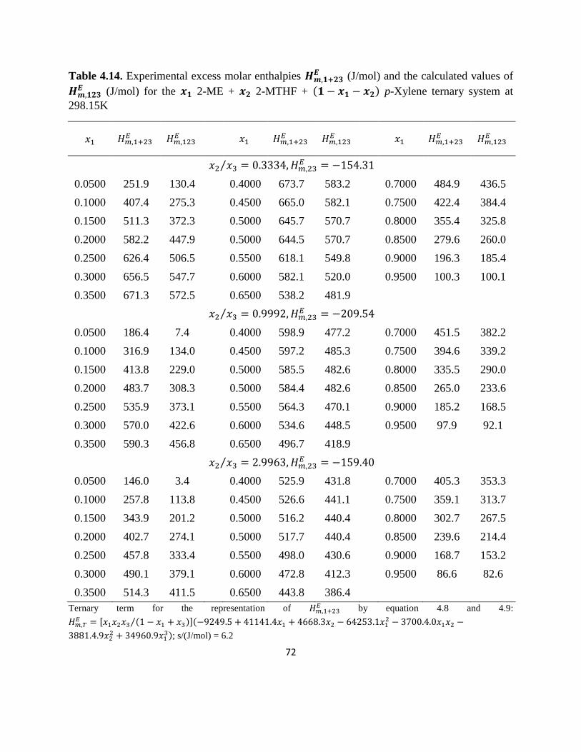
72
Table 4.14. Experimental excess molar enthalpies (J/mol) and the calculated values of
(J/mol) for the 2-ME + 2-MTHF + p-Xylene ternary system at
298.15K
⁄
0.0500 251.9 130.4
0.4000 673.7 583.2
0.7000 484.9 436.5
0.1000 407.4 275.3
0.4500 665.0 582.1
0.7500 422.4 384.4
0.1500 511.3 372.3
0.5000 645.7 570.7
0.8000 355.4 325.8
0.2000 582.2 447.9
0.5000 644.5 570.7
0.8500 279.6 260.0
0.2500 626.4 506.5
0.5500 618.1 549.8
0.9000 196.3 185.4
0.3000 656.5 547.7
0.6000 582.1 520.0
0.9500 100.3 100.1
0.3500 671.3 572.5
0.6500 538.2 481.9
⁄
0.0500 186.4 7.4
0.4000 598.9 477.2
0.7000 451.5 382.2
0.1000 316.9 134.0
0.4500 597.2 485.3
0.7500 394.6 339.2
0.1500 413.8 229.0
0.5000 585.5 482.6
0.8000 335.5 290.0
0.2000 483.7 308.3
0.5000 584.4 482.6
0.8500 265.0 233.6
0.2500 535.9 373.1
0.5500 564.3 470.1
0.9000 185.2 168.5
0.3000 570.0 422.6
0.6000 534.6 448.5
0.9500 97.9 92.1
0.3500 590.3 456.8
0.6500 496.7 418.9
⁄
0.0500 146.0 3.4
0.4000 525.9 431.8
0.7000 405.3 353.3
0.1000 257.8 113.8
0.4500 526.6 441.1
0.7500 359.1 313.7
0.1500 343.9 201.2
0.5000 516.2 440.4
0.8000 302.7 267.5
0.2000 402.7 274.1
0.5000 517.7 440.4
0.8500 239.6 214.4
0.2500 457.8 333.4
0.5500 498.0 430.6
0.9000 168.7 153.2
0.3000 490.1 379.1
0.6000 472.8 412.3
0.9500 86.6 82.6
0.3500 514.3 411.5 0.6500 443.8 386.4
Ternary term for the representation of by equation 4.8 and 4.9:
[ ⁄ ]
; s/(J/mol) = 6.2
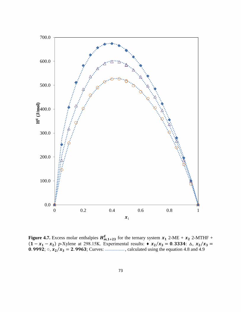
73
Figure 4.7. Excess molar enthalpies for the ternary system 2-ME + 2-MTHF +
p-Xylene at 298.15K. Experimental results: ♦ ⁄ : , ⁄ ; , ⁄ ; Curves: , calculated using the equation 4.8 and 4.9
0.0
100.0
200.0
300.0
400.0
500.0
600.0
700.0
0 0.2 0.4 0.6 0.8 1
HE (
J/m
ol)
𝒙1
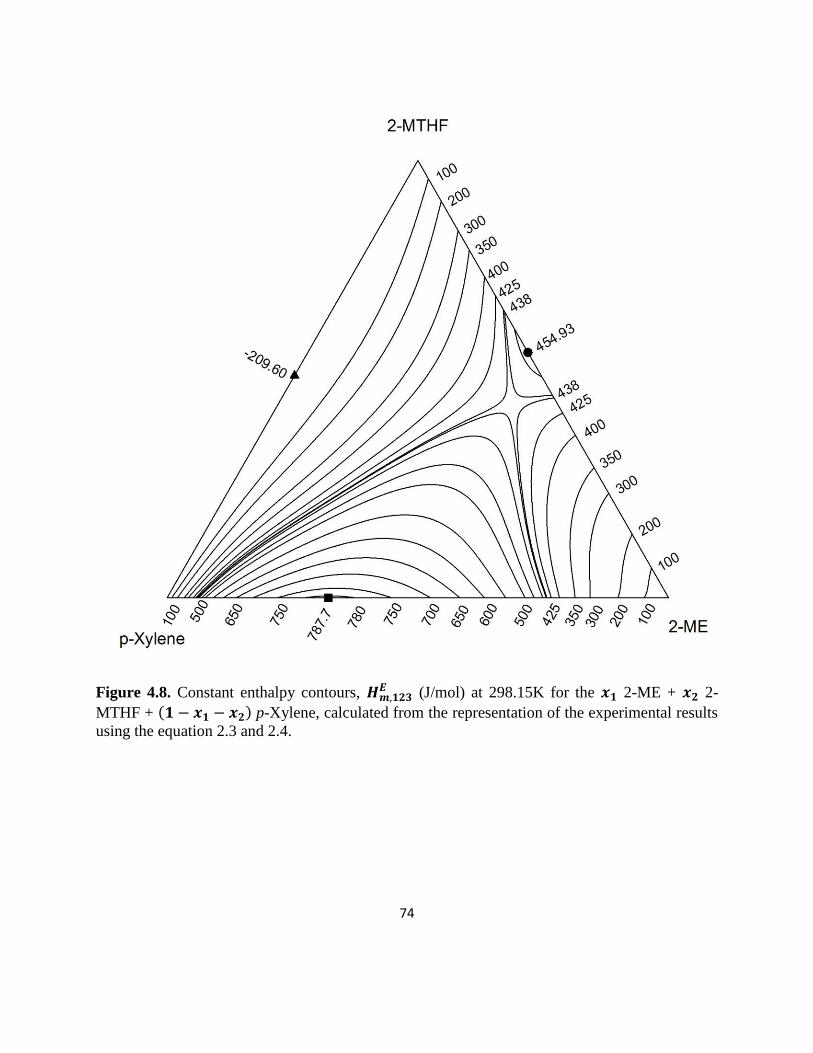
74
Figure 4.8. Constant enthalpy contours, (J/mol) at 298.15K for the 2-ME + 2-
MTHF + p-Xylene, calculated from the representation of the experimental results
using the equation 2.3 and 2.4.
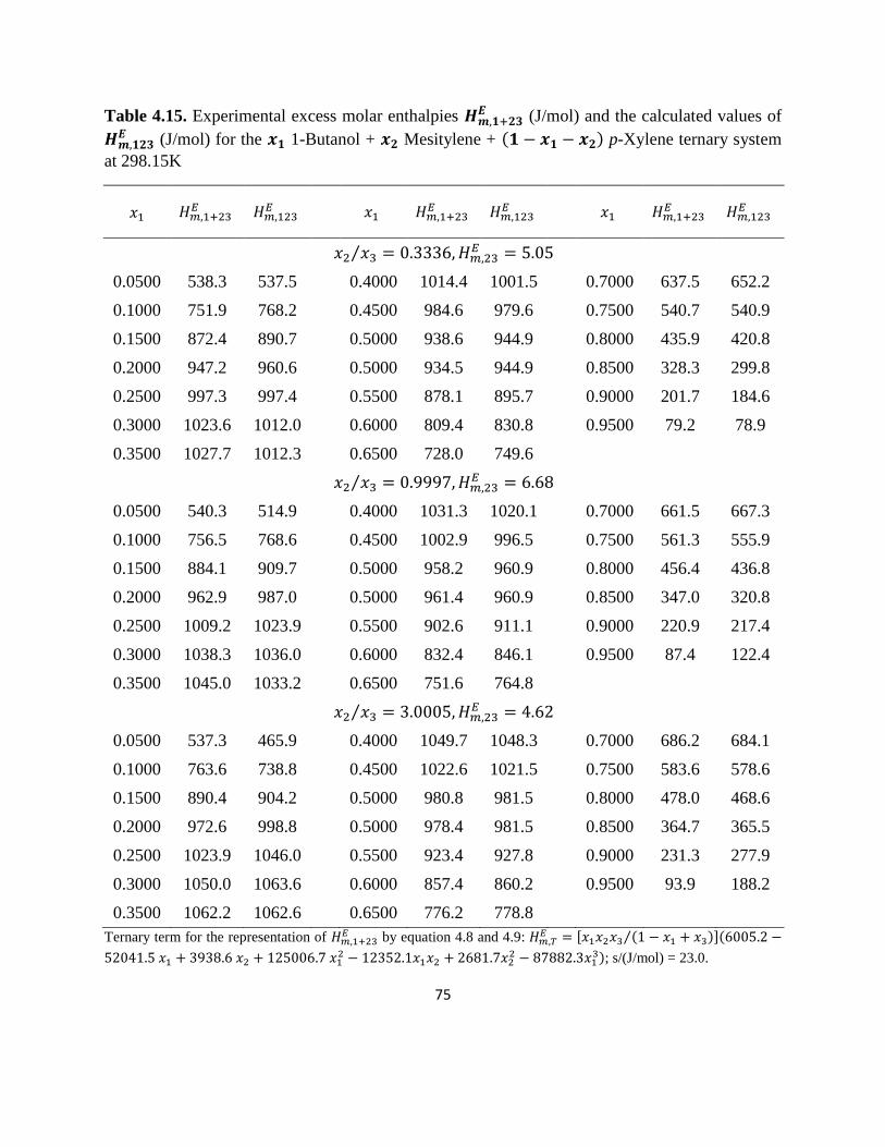
75
Table 4.15. Experimental excess molar enthalpies (J/mol) and the calculated values of
(J/mol) for the 1-Butanol + Mesitylene + p-Xylene ternary system
at 298.15K
⁄
0.0500 538.3 537.5
0.4000 1014.4 1001.5
0.7000 637.5 652.2
0.1000 751.9 768.2
0.4500 984.6 979.6
0.7500 540.7 540.9
0.1500 872.4 890.7
0.5000 938.6 944.9
0.8000 435.9 420.8
0.2000 947.2 960.6
0.5000 934.5 944.9
0.8500 328.3 299.8
0.2500 997.3 997.4
0.5500 878.1 895.7
0.9000 201.7 184.6
0.3000 1023.6 1012.0
0.6000 809.4 830.8
0.9500 79.2 78.9
0.3500 1027.7 1012.3
0.6500 728.0 749.6
⁄
0.0500 540.3 514.9
0.4000 1031.3 1020.1
0.7000 661.5 667.3
0.1000 756.5 768.6
0.4500 1002.9 996.5
0.7500 561.3 555.9
0.1500 884.1 909.7
0.5000 958.2 960.9
0.8000 456.4 436.8
0.2000 962.9 987.0
0.5000 961.4 960.9
0.8500 347.0 320.8
0.2500 1009.2 1023.9
0.5500 902.6 911.1
0.9000 220.9 217.4
0.3000 1038.3 1036.0
0.6000 832.4 846.1
0.9500 87.4 122.4
0.3500 1045.0 1033.2
0.6500 751.6 764.8
⁄
0.0500 537.3 465.9
0.4000 1049.7 1048.3
0.7000 686.2 684.1
0.1000 763.6 738.8
0.4500 1022.6 1021.5
0.7500 583.6 578.6
0.1500 890.4 904.2
0.5000 980.8 981.5
0.8000 478.0 468.6
0.2000 972.6 998.8
0.5000 978.4 981.5
0.8500 364.7 365.5
0.2500 1023.9 1046.0
0.5500 923.4 927.8
0.9000 231.3 277.9
0.3000 1050.0 1063.6
0.6000 857.4 860.2
0.9500 93.9 188.2
0.3500 1062.2 1062.6 0.6500 776.2 778.8
Ternary term for the representation of by equation 4.8 and 4.9:
[ ⁄ ]
; s/(J/mol) = 23.0.
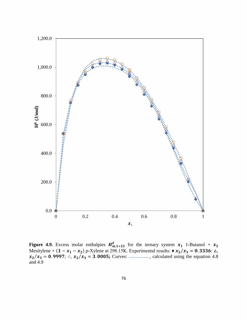
76
Figure 4.9. Excess molar enthalpies for the ternary system 1-Butanol +
Mesitylene + p-Xylene at 298.15K. Experimental results: ♦ ⁄ : ,
⁄ ; , ⁄ ; Curves: , calculated using the equation 4.8
and 4.9
0.0
200.0
400.0
600.0
800.0
1,000.0
1,200.0
0 0.2 0.4 0.6 0.8 1
HE (
J/m
ol)
𝒙1
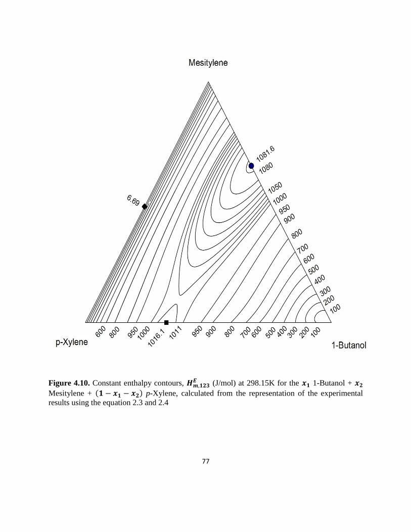
77
Figure 4.10. Constant enthalpy contours, (J/mol) at 298.15K for the 1-Butanol +
Mesitylene + p-Xylene, calculated from the representation of the experimental
results using the equation 2.3 and 2.4
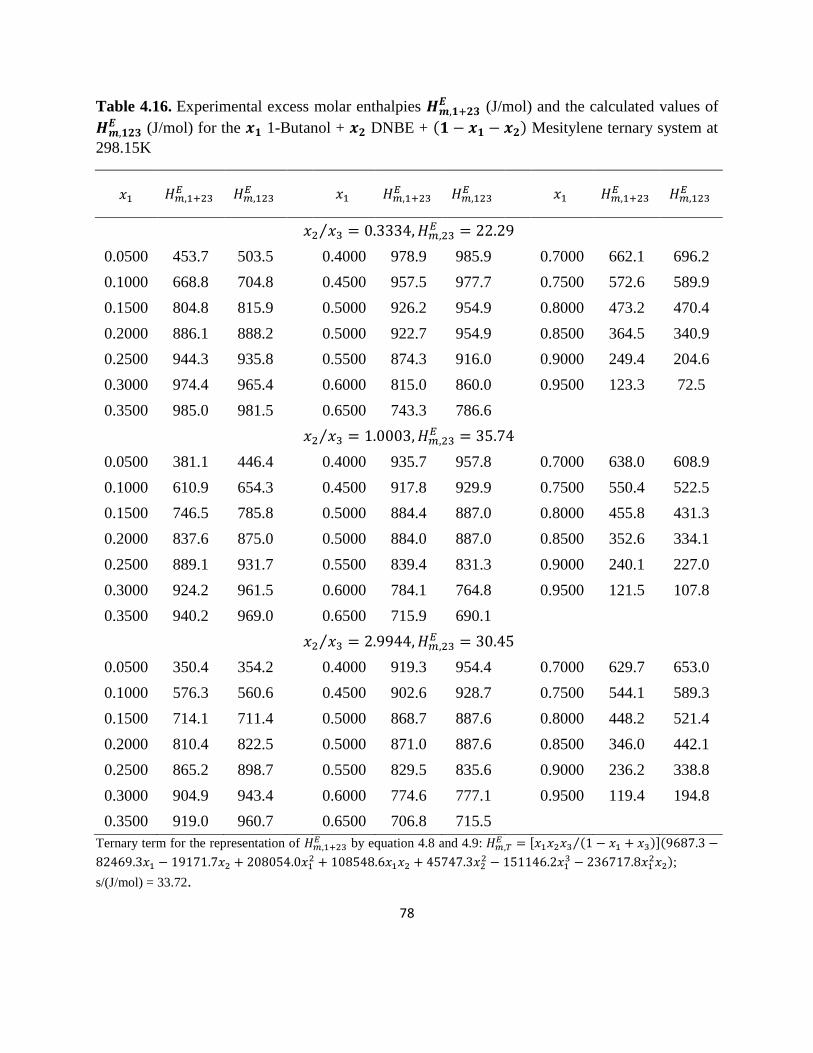
78
Table 4.16. Experimental excess molar enthalpies (J/mol) and the calculated values of
(J/mol) for the 1-Butanol + DNBE + Mesitylene ternary system at
298.15K
⁄
0.0500 453.7 503.5
0.4000 978.9 985.9
0.7000 662.1 696.2
0.1000 668.8 704.8
0.4500 957.5 977.7
0.7500 572.6 589.9
0.1500 804.8 815.9
0.5000 926.2 954.9
0.8000 473.2 470.4
0.2000 886.1 888.2
0.5000 922.7 954.9
0.8500 364.5 340.9
0.2500 944.3 935.8
0.5500 874.3 916.0
0.9000 249.4 204.6
0.3000 974.4 965.4
0.6000 815.0 860.0
0.9500 123.3 72.5
0.3500 985.0 981.5
0.6500 743.3 786.6
⁄
0.0500 381.1 446.4
0.4000 935.7 957.8
0.7000 638.0 608.9
0.1000 610.9 654.3
0.4500 917.8 929.9
0.7500 550.4 522.5
0.1500 746.5 785.8
0.5000 884.4 887.0
0.8000 455.8 431.3
0.2000 837.6 875.0
0.5000 884.0 887.0
0.8500 352.6 334.1
0.2500 889.1 931.7
0.5500 839.4 831.3
0.9000 240.1 227.0
0.3000 924.2 961.5
0.6000 784.1 764.8
0.9500 121.5 107.8
0.3500 940.2 969.0
0.6500 715.9 690.1
⁄
0.0500 350.4 354.2
0.4000 919.3 954.4
0.7000 629.7 653.0
0.1000 576.3 560.6
0.4500 902.6 928.7
0.7500 544.1 589.3
0.1500 714.1 711.4
0.5000 868.7 887.6
0.8000 448.2 521.4
0.2000 810.4 822.5
0.5000 871.0 887.6
0.8500 346.0 442.1
0.2500 865.2 898.7
0.5500 829.5 835.6
0.9000 236.2 338.8
0.3000 904.9 943.4
0.6000 774.6 777.1
0.9500 119.4 194.8
0.3500 919.0 960.7 0.6500 706.8 715.5
Ternary term for the representation of by equation 4.8 and 4.9:
[ ⁄ ]
;
s/(J/mol) = 33.72.
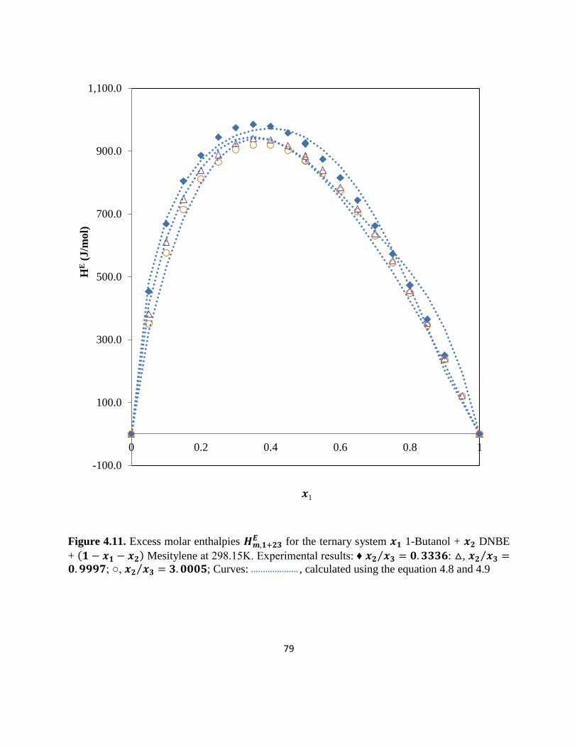
79
Figure 4.11. Excess molar enthalpies for the ternary system 1-Butanol + DNBE
+ Mesitylene at 298.15K. Experimental results: ♦ ⁄ : , ⁄ ; , ⁄ ; Curves: , calculated using the equation 4.8 and 4.9
-100.0
100.0
300.0
500.0
700.0
900.0
1,100.0
0 0.2 0.4 0.6 0.8 1
HE (
J/m
ol)
𝒙1
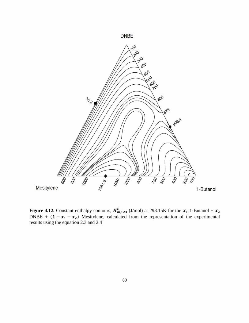
80
Figure 4.12. Constant enthalpy contours, (J/mol) at 298.15K for the 1-Butanol +
DNBE + Mesitylene, calculated from the representation of the experimental
results using the equation 2.3 and 2.4
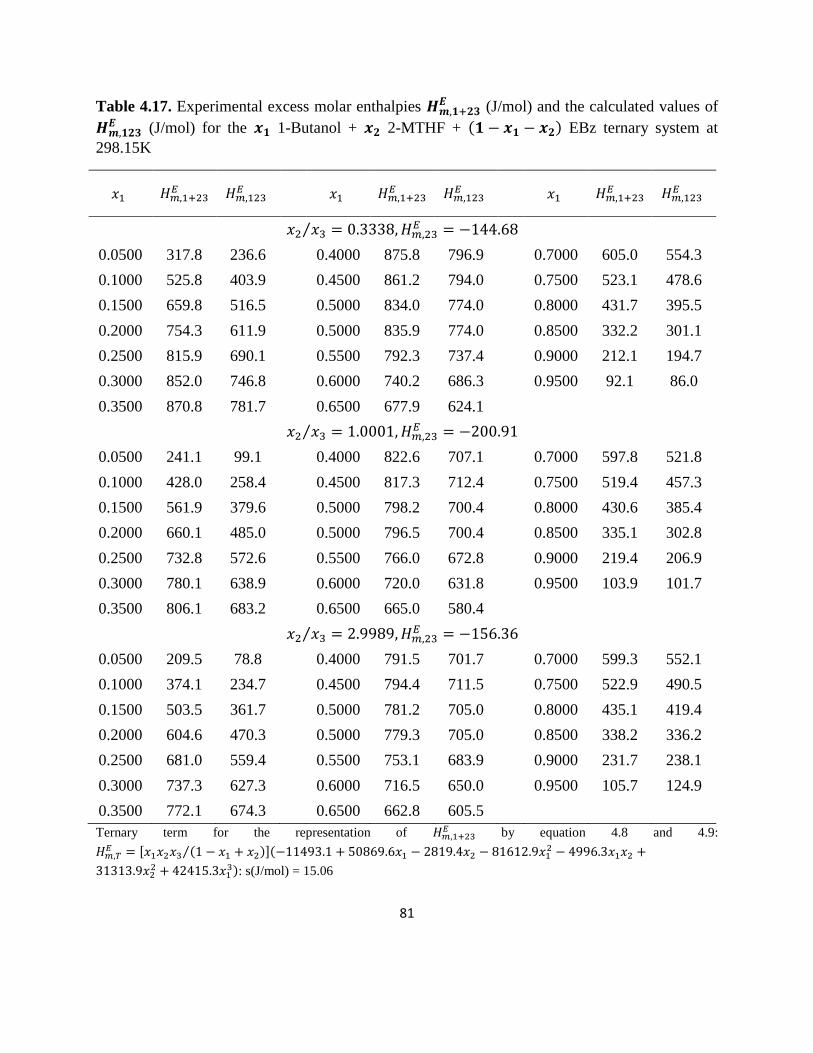
81
Table 4.17. Experimental excess molar enthalpies (J/mol) and the calculated values of
(J/mol) for the 1-Butanol + 2-MTHF + EBz ternary system at
298.15K
⁄
0.0500 317.8 236.6
0.4000 875.8 796.9
0.7000 605.0 554.3
0.1000 525.8 403.9
0.4500 861.2 794.0
0.7500 523.1 478.6
0.1500 659.8 516.5
0.5000 834.0 774.0
0.8000 431.7 395.5
0.2000 754.3 611.9
0.5000 835.9 774.0
0.8500 332.2 301.1
0.2500 815.9 690.1
0.5500 792.3 737.4
0.9000 212.1 194.7
0.3000 852.0 746.8
0.6000 740.2 686.3
0.9500 92.1 86.0
0.3500 870.8 781.7
0.6500 677.9 624.1
⁄
0.0500 241.1 99.1
0.4000 822.6 707.1
0.7000 597.8 521.8
0.1000 428.0 258.4
0.4500 817.3 712.4
0.7500 519.4 457.3
0.1500 561.9 379.6
0.5000 798.2 700.4
0.8000 430.6 385.4
0.2000 660.1 485.0
0.5000 796.5 700.4
0.8500 335.1 302.8
0.2500 732.8 572.6
0.5500 766.0 672.8
0.9000 219.4 206.9
0.3000 780.1 638.9
0.6000 720.0 631.8
0.9500 103.9 101.7
0.3500 806.1 683.2
0.6500 665.0 580.4
⁄
0.0500 209.5 78.8
0.4000 791.5 701.7
0.7000 599.3 552.1
0.1000 374.1 234.7
0.4500 794.4 711.5
0.7500 522.9 490.5
0.1500 503.5 361.7
0.5000 781.2 705.0
0.8000 435.1 419.4
0.2000 604.6 470.3
0.5000 779.3 705.0
0.8500 338.2 336.2
0.2500 681.0 559.4
0.5500 753.1 683.9
0.9000 231.7 238.1
0.3000 737.3 627.3
0.6000 716.5 650.0
0.9500 105.7 124.9
0.3500 772.1 674.3 0.6500 662.8 605.5
Ternary term for the representation of by equation 4.8 and 4.9:
[ ⁄ ]
: s(J/mol) = 15.06
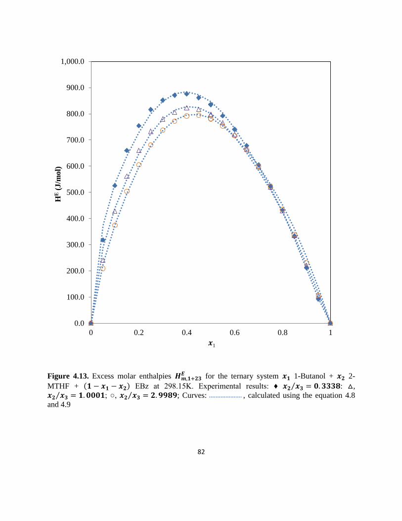
82
Figure 4.13. Excess molar enthalpies for the ternary system 1-Butanol + 2-
MTHF + EBz at 298.15K. Experimental results: ♦ ⁄ : ,
⁄ ; , ⁄ ; Curves: , calculated using the equation 4.8
and 4.9
0.0
100.0
200.0
300.0
400.0
500.0
600.0
700.0
800.0
900.0
1,000.0
0 0.2 0.4 0.6 0.8 1
HE (
J/m
ol)
𝒙1
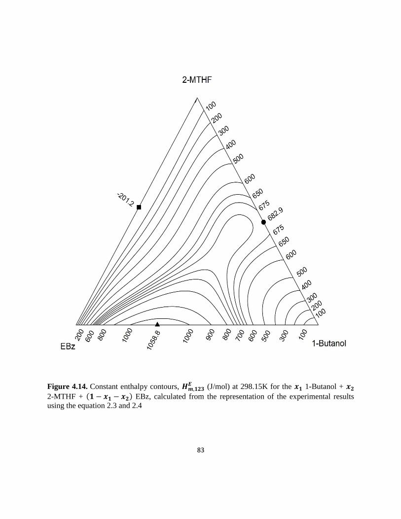
83
Figure 4.14. Constant enthalpy contours, (J/mol) at 298.15K for the 1-Butanol +
2-MTHF + EBz, calculated from the representation of the experimental results
using the equation 2.3 and 2.4
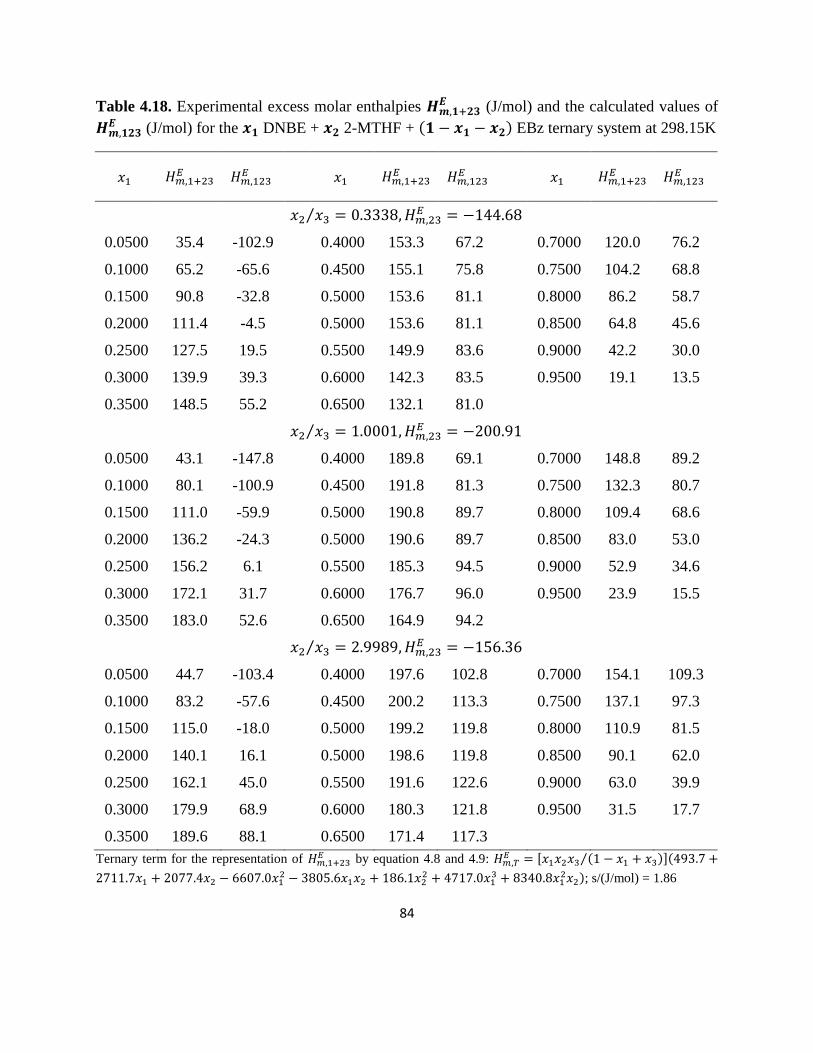
84
Table 4.18. Experimental excess molar enthalpies (J/mol) and the calculated values of
(J/mol) for the DNBE + 2-MTHF + EBz ternary system at 298.15K
⁄
0.0500 35.4 -102.9
0.4000 153.3 67.2
0.7000 120.0 76.2
0.1000 65.2 -65.6
0.4500 155.1 75.8
0.7500 104.2 68.8
0.1500 90.8 -32.8
0.5000 153.6 81.1
0.8000 86.2 58.7
0.2000 111.4 -4.5
0.5000 153.6 81.1
0.8500 64.8 45.6
0.2500 127.5 19.5
0.5500 149.9 83.6
0.9000 42.2 30.0
0.3000 139.9 39.3
0.6000 142.3 83.5
0.9500 19.1 13.5
0.3500 148.5 55.2
0.6500 132.1 81.0
⁄
0.0500 43.1 -147.8
0.4000 189.8 69.1
0.7000 148.8 89.2
0.1000 80.1 -100.9
0.4500 191.8 81.3
0.7500 132.3 80.7
0.1500 111.0 -59.9
0.5000 190.8 89.7
0.8000 109.4 68.6
0.2000 136.2 -24.3
0.5000 190.6 89.7
0.8500 83.0 53.0
0.2500 156.2 6.1
0.5500 185.3 94.5
0.9000 52.9 34.6
0.3000 172.1 31.7
0.6000 176.7 96.0
0.9500 23.9 15.5
0.3500 183.0 52.6
0.6500 164.9 94.2
⁄
0.0500 44.7 -103.4
0.4000 197.6 102.8
0.7000 154.1 109.3
0.1000 83.2 -57.6
0.4500 200.2 113.3
0.7500 137.1 97.3
0.1500 115.0 -18.0
0.5000 199.2 119.8
0.8000 110.9 81.5
0.2000 140.1 16.1
0.5000 198.6 119.8
0.8500 90.1 62.0
0.2500 162.1 45.0
0.5500 191.6 122.6
0.9000 63.0 39.9
0.3000 179.9 68.9
0.6000 180.3 121.8
0.9500 31.5 17.7
0.3500 189.6 88.1 0.6500 171.4 117.3
Ternary term for the representation of by equation 4.8 and 4.9:
[ ⁄ ]
; s/(J/mol) = 1.86
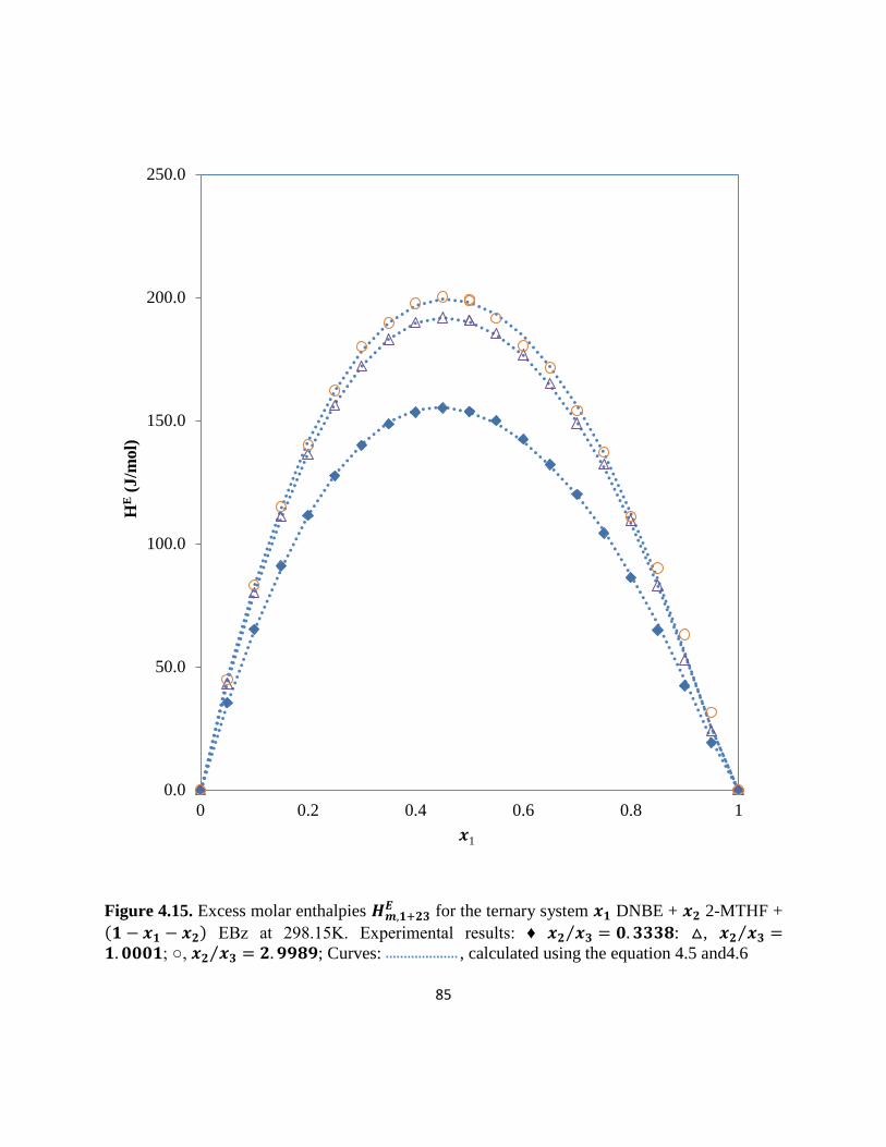
85
Figure 4.15. Excess molar enthalpies for the ternary system DNBE + 2-MTHF +
EBz at 298.15K. Experimental results: ♦ ⁄ : , ⁄ ; , ⁄ ; Curves: , calculated using the equation 4.5 and4.6
0.0
50.0
100.0
150.0
200.0
250.0
0 0.2 0.4 0.6 0.8 1
HE (
J/m
ol)
𝒙1
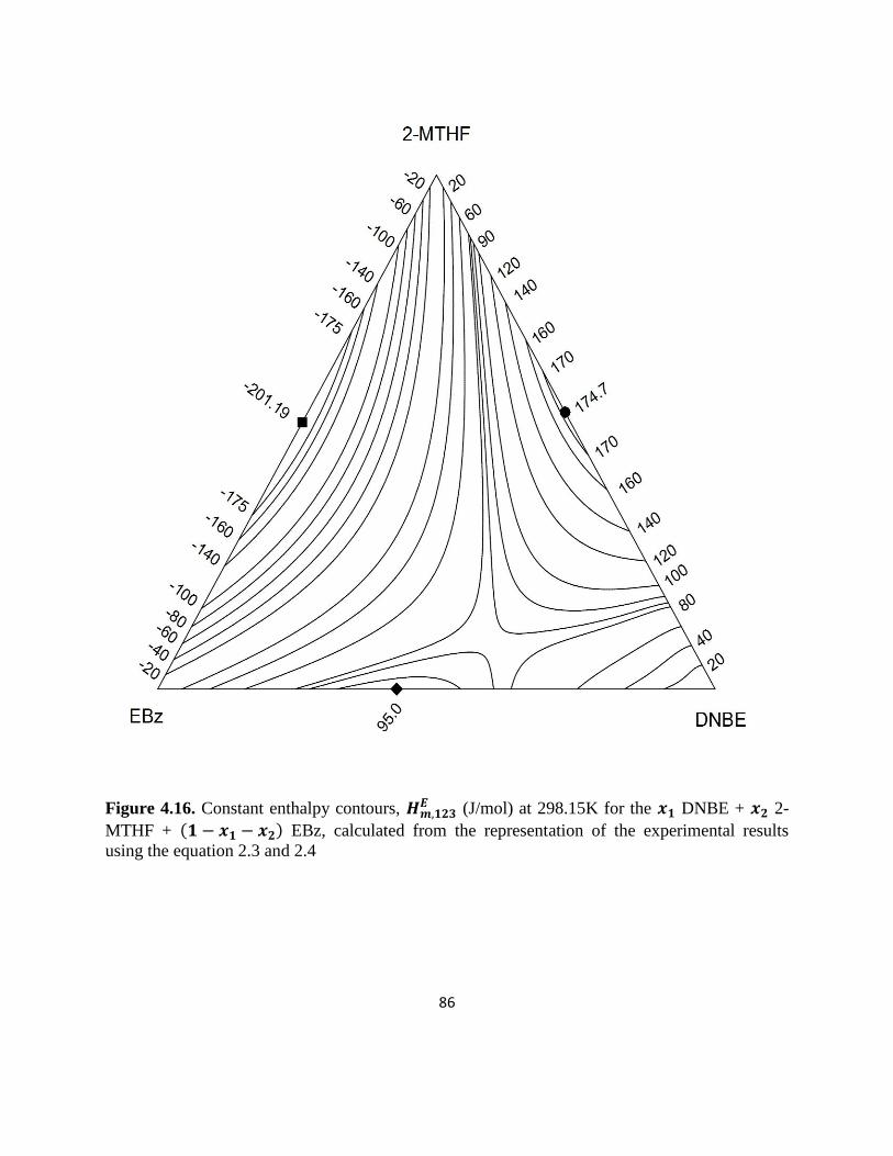
86
Figure 4.16. Constant enthalpy contours, (J/mol) at 298.15K for the DNBE + 2-
MTHF + EBz, calculated from the representation of the experimental results
using the equation 2.3 and 2.4
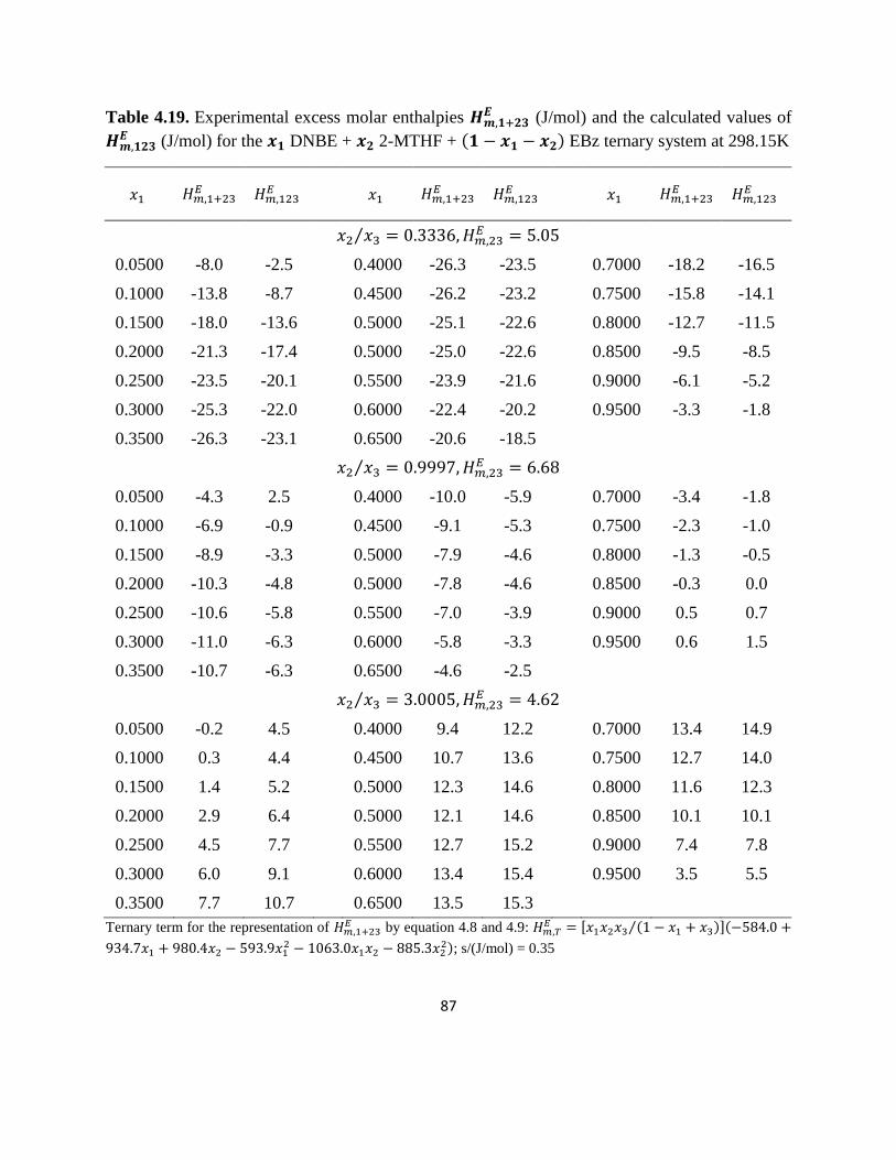
87
Table 4.19. Experimental excess molar enthalpies (J/mol) and the calculated values of
(J/mol) for the DNBE + 2-MTHF + EBz ternary system at 298.15K
⁄
0.0500 -8.0 -2.5
0.4000 -26.3 -23.5
0.7000 -18.2 -16.5
0.1000 -13.8 -8.7
0.4500 -26.2 -23.2
0.7500 -15.8 -14.1
0.1500 -18.0 -13.6
0.5000 -25.1 -22.6
0.8000 -12.7 -11.5
0.2000 -21.3 -17.4
0.5000 -25.0 -22.6
0.8500 -9.5 -8.5
0.2500 -23.5 -20.1
0.5500 -23.9 -21.6
0.9000 -6.1 -5.2
0.3000 -25.3 -22.0
0.6000 -22.4 -20.2
0.9500 -3.3 -1.8
0.3500 -26.3 -23.1
0.6500 -20.6 -18.5
⁄
0.0500 -4.3 2.5
0.4000 -10.0 -5.9
0.7000 -3.4 -1.8
0.1000 -6.9 -0.9
0.4500 -9.1 -5.3
0.7500 -2.3 -1.0
0.1500 -8.9 -3.3
0.5000 -7.9 -4.6
0.8000 -1.3 -0.5
0.2000 -10.3 -4.8
0.5000 -7.8 -4.6
0.8500 -0.3 0.0
0.2500 -10.6 -5.8
0.5500 -7.0 -3.9
0.9000 0.5 0.7
0.3000 -11.0 -6.3
0.6000 -5.8 -3.3
0.9500 0.6 1.5
0.3500 -10.7 -6.3
0.6500 -4.6 -2.5
⁄
0.0500 -0.2 4.5
0.4000 9.4 12.2
0.7000 13.4 14.9
0.1000 0.3 4.4
0.4500 10.7 13.6
0.7500 12.7 14.0
0.1500 1.4 5.2
0.5000 12.3 14.6
0.8000 11.6 12.3
0.2000 2.9 6.4
0.5000 12.1 14.6
0.8500 10.1 10.1
0.2500 4.5 7.7
0.5500 12.7 15.2
0.9000 7.4 7.8
0.3000 6.0 9.1
0.6000 13.4 15.4
0.9500 3.5 5.5
0.3500 7.7 10.7 0.6500 13.5 15.3
Ternary term for the representation of by equation 4.8 and 4.9:
[ ⁄ ]
; s/(J/mol) = 0.35
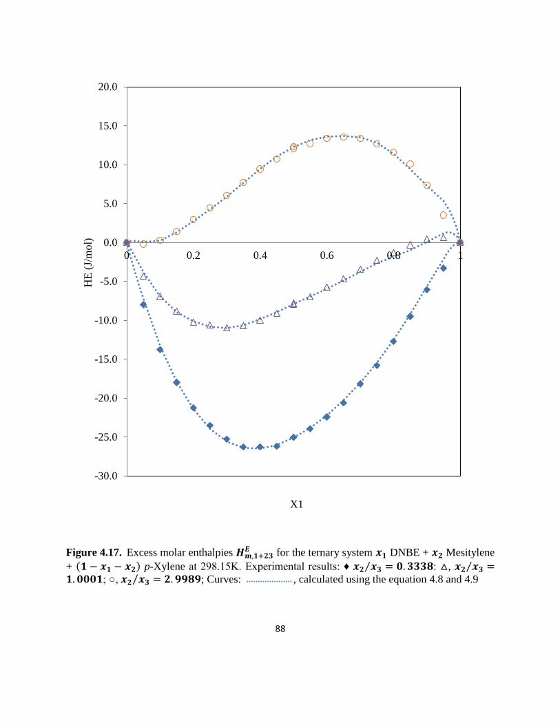
88
Figure 4.17. Excess molar enthalpies for the ternary system DNBE + Mesitylene
+ p-Xylene at 298.15K. Experimental results: ♦ ⁄ : , ⁄ ; , ⁄ ; Curves: , calculated using the equation 4.8 and 4.9
-30.0
-25.0
-20.0
-15.0
-10.0
-5.0
0.0
5.0
10.0
15.0
20.0
0 0.2 0.4 0.6 0.8 1
HE
(J/
mo
l)
X1
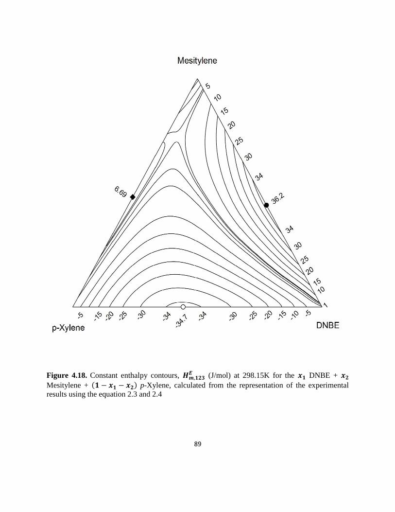
89
Figure 4.18. Constant enthalpy contours, (J/mol) at 298.15K for the DNBE +
Mesitylene + p-Xylene, calculated from the representation of the experimental
results using the equation 2.3 and 2.4
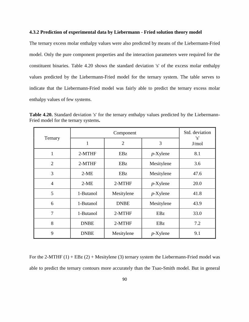
90
4.3.2 Prediction of experimental data by Liebermann - Fried solution theory model
The ternary excess molar enthalpy values were also predicted by means of the Liebermann-Fried
model. Only the pure component properties and the interaction parameters were required for the
constituent binaries. Table 4.20 shows the standard deviation 's' of the excess molar enthalpy
values predicted by the Liebermann-Fried model for the ternary system. The table serves to
indicate that the Liebermann-Fried model was fairly able to predict the ternary excess molar
enthalpy values of few systems.
Table 4.20. Standard deviation 's' for the ternary enthalpy values predicted by the Liebermann-
Fried model for the ternary systems.
Ternary Component Std. deviation
's'
J/mol 1 2 3
1 2-MTHF EBz p-Xylene 8.1
2 2-MTHF EBz Mesitylene 3.6
3 2-ME EBz Mesitylene 47.6
4 2-ME 2-MTHF p-Xylene 20.0
5 1-Butanol Mesitylene p-Xylene 41.8
6 1-Butanol DNBE Mesitylene 43.9
7 1-Butanol 2-MTHF EBz 33.0
8 DNBE 2-MTHF EBz 7.2
9 DNBE Mesitylene p-Xylene 9.1
For the 2-MTHF (1) + EBz (2) + Mesitylene (3) ternary system the Liebermann-Fried model was
able to predict the ternary contours more accurately than the Tsao-Smith model. But in general
91
the Liebermann-fried model was not that successful in predicting the ternary contours. No
internal maximum exists for all the nine ternary systems. An internal saddle points exists for the
2-ME (1) + 2-MTHF (2) + p-Xylene (3), (1-Butanol or DNBE) (1) + 2-MTHF (2) + EBz (3)
ternary systems. The standard deviation is relatively higher for the ternary systems involving 1-
Butanol and 2-ME as the component 1.
92
5.0 CONCLUSIONS AND RECOMMENDATIONS
5.1 Conclusions
The experimental excess molar enthalpy values for 15 binaries and nine ternary systems at
298.15K have been satisfactorily carried out using an LKB (10700-1) flow microcalorimeter.
The following conclusions can be drawn based on the results obtained in this study.
The binary mixtures studied shows, systems exhibiting positive and negative excess
molar enthalpy values. The reason for exothermic and endothermic mixing behavior of
specific mixtures was analyzed in this study.
The Liebermann-Fried model was able to represent the experimental excess molar
enthalpy of some binary and ternary systems with reasonable accuracy with a standard
deviation ranging from 0.3 - 59.5 J/mol for the binary systems and 3.6 - 47.6 J/mol for
the ternary systems.
The Tsao-Smith model was closely able to represent the excess molar enthalpy of all
ternary systems except the 1-Butanol ternary system.
The Liebermann-fried model was able to predict the ternary excess molar enthalpies of
(2-MTHF + hydrocarbons) and (DNBE + 2-MTHF + EBz) ternary systems, for the other
seven ternary systems the model predicts the enthalpy values with high standard
deviation.
93
5.2 Recommendations
Following recommendations are suggested for future studies.
Vapor liquid equilibrium (VLE) values for the binary systems studied in this research
work can be experimentally measured. The measured values can be compared with the
values calculated using the Liebermann-Fried model binary interaction parameters,
determined in this study.
Out of the possible 35 ternary systems involving the chosen seven chemicals, nine
ternary systems have been studied in this research work. It would be interesting to study
the excess molar enthalpy of the other 26 ternary systems.
For further studies it is desirable to apply other thermodynamic models to predict the
binary and ternary excess molar enthalpies values measured in this research work and
can be compared with the models used in this study.
94
6.0 REFERENCES
Abe, A., Flory, P. (1965). The thermodynamic properties of mixtures of small, nonpolar
molecules. Journal of the American Chemical Society, 87(9), 1838-1846.
Abrams, D. S., Prausnitz, J. M. (1975). Statistical thermodynamics of liquid mixtures: a new
expression for the excess Gibbs energy of partly or completely miscible systems. AIChE
Journal, 21(1), 116-128.
Aicart, E., Junquera, E., Letcher, T. M. (1995). Isobaric thermal expansivity and isothermal
compressibility of several nonsaturated hydrocarbons at 298.15 K. Journal of Chemical
and Engineering Data, 40(6), 1225-1227.
Ancillotti, F., Fattore, V. (1998). Oxygenate fuels: Market expansion and catalytic aspect of
synthesis. Fuel Processing Technology, 57(3), 163-194.
Baud, M. (1915). Thermal analysis of binary mixtures. Bull. Soc. Chim. Fr, 17, 329-345.
Bauer, N. (1959). Determination of Density. Physical Methods of Organic Chemistry, Part I;
Arnold Weissberger. editor, Interscience: New York, 1959, chapter IV.
Bevington, P. R., Robinson, D. K. (2003). Data reduction and error analysis for the physical
sciences. Data reduction and error analysis for the physical sciences; McGraw-Hill,
New York, 2003.
Bose, E. (1907). Calorimetric studies. Z. Phys. Chem, 58, 585-624.
Brandreth, D. A., O'Neill, S. P., Missen, R. W. (1966). Thermodynamic excess functions of
binary solutions involving a fluoroalcohol. Transactions of the Faraday Society, 62(0),
2355-2366.
95
CEPA. (1990). Ministry of Justice Retrieved from http://laws-lois.justice.gc.ca/PDF/SOR-90-
247.pdf.
Cerdeiri a, C. ., Tovar, C. ., Gonz lez, D., Carballo, E., Roman , . (2001). Thermodynamics
of the nitromethane + 1-butanol system near the upper critical point. Fluid Phase
Equilibria, 179(1–2), 101-115.
Christensen, J., Hansen, L., Eatough, D., Izatt, R., Hart, R. (1976). Isothermal high pressure flow
calorimeter. Review of Scientific Instruments, 47(6), 730-734.
Christensen, J. J., Johnston, H. D., Izatt, R. M. (1968). An Isothermal Titration Calorimeter.
Review of Scientific Instruments, 39(9), 1356-1359.
Clarke, B. (1905). Determination of Several Heats of Mixing. Phys. Z, 5, 154-159.
Cobos, J. C., Garcia, I., Gonzalez, J. A., Casanova, C. (1988). Excess enthalpy. 2-
Methoxyethanol - 1-butanol system. International DATA Series, Selected Data on
Mixtures, Series A: Thermodynamic Properties of Non-Reacting Binary Systems of
Organic Substances(2), 85.
Davis, J. M., Farland, W. H. (2001). The paradoxes of MTBE. Toxicological Sciences, 61(2),
211-217.
Elliott, K., Wormald, C. J. (1976). A precision differential flow calorimeter the excess enthalpy
of benzene + cyclohexane between 280.15 K and 393.15 K. The Journal of Chemical
Thermodynamics, 8(9), 881-893.
Flory, P. (1965). Statistical thermodynamics of liquid mixtures. Journal of the American
Chemical Society, 87(9), 1833-1838.
96
Francesconi, R., Comelli, F. (1997). Excess Molar Enthalpies, Densities, and Excess Molar
Volumes of Diethyl Carbonate in Binary Mixtures with Seven n-Alkanols at 298.15 K.
Journal of Chemical and Engineering Data, 42(1), 45-48.
George, J., Sastry, N. V. (2003). Densities, excess molar volumes, viscosities, speeds of sound,
excess isentropic compressibilities, and relative permittivities for CmH2m + 1 (OCH2CH2)n
OH (m= 1 or 2 or 4 and n= 1) + benzene, + toluene, + (o-, m-, and p-) xylenes,+
ethylbenzene, and + cyclohexane. Journal of Chemical and Engineering Data, 48(4),
977-989.
Gill, P., Moghadam, T. T., Ranjbar, B. (2010). Differential scanning calorimetry techniques:
applications in biology and nanoscience. Journal of biomolecular techniques: JBT, 21(4),
167.
Giner, B., Artigas, H., Carrion, A., Lafuente, C., Royo, F. (2003). Excess thermodynamic
properties of isomeric butanols with 2-methyl-tetrahydrofuran. Journal of molecular
liquids, 108(1-3), 303-311.
Harsted, B. S., Thomsen, E. S. (1974). Excess enthalpies from flow microcalorimetry 1.
Experimental method and excess enthalpies for carbon tetrachloride + cyclohexane,
+benzene, and +octamethylcyclotetrasiloxane, and of n-hexane + cyclohexane. The
Journal of Chemical Thermodynamics, 6(6), 549-555.
Hassan, S. M. N. (2010). Excess molar enthalpies of binary and ternary systems involving
hydrocarbons and ethers. (Master of Science), University of Saskatchewan, Saskatoon.
97
Hirobe, H. I. (1925). Thermochemical studies II. The thermochemistry of concentrated solution.
The Journal of the College of Science, Imperial University of Tokyo, 1, 155-222.
Höhne, G., Hemminger, W., Flammersheim. H.-J. (2003). Differential scanning calorimetry:
Springer
Holt, D. L., Smith, B. D. (1974). Measurement of excess enthalpies with Tronac titration
calorimeter. Data for some C8 aromatic binaries. Journal of Chemical and Engineering
Data, 19(2), 129-133.
Hsu, K.-Y., Lawrence Clever, H. (1975). The excess enthalpies of the 15 binary mixtures formed
from cyclohexane, benzene, toluene, 1, 4-dimethylbenzene, 1, 2, 4-trimethylbenzene, and
1, 3, 5-trimethylbenzene at 298.15 K. The Journal of Chemical Thermodynamics, 7(5),
435-442.
Jablonski, P., Müller-Blecking, A., Borchard, W. (2003). A method to determine mixing
enthalpies by DSC. Journal of Thermal Analysis and Calorimetry, 74(3), 779-787.
Kammerer, K., Lichtenthaler, R. (1998). Excess properties of binary alkanol–ether mixtures and
the application of the ERAS model. Thermochimica Acta, 310(1), 61-67.
Kimura, F., Benson, G. C., Halpin, C. J. (1983). Excess enthalpies of binary mixtures of n-
heptane with hexane isomers. Fluid Phase Equilibria, 11(3), 245-250.
Kinart, C., Kinart, W., Ćwiklińska, . (2002). 2-Methoxyethanol–Tetrahydrofuran–Binary
Liquid System. Viscosities, densities, excess molar volumes and excess Gibbs activation
energies of viscous flow at various temperatures. Journal of Thermal Analysis and
Calorimetry, 68(1), 307-317.
98
Lasdon, L. S., Waren, A. D., Jain, A., Ratner, M. (1978). Design and testing of a generalized
reduced gradient code for nonlinear programming. ACM Transactions on Mathematical
Software (TOMS), 4(1), 34-50.
Liao, W.-C., Lin, H.-M., Lee, M.-J. (2009a). Excess Molar Enthalpies of Binary Systems of 2-
Octanone or 3-Octanone with Dodecane, Tetradecane, or Hexadecane at 298.15 K.
Journal of Chemical and Engineering Data, 55(1), 217-222.
Liao, W.-C., Lin, H.-M., Lee, M.-J. (2009b). Excess Molar Enthalpies of Binary Systems of n-
Valeric Anhydride or n-Hexanoic Anhydride with n-Dodecane, n-Tetradecane, or n-
Hexadecane at 298.15 K. Journal of Chemical and Engineering Data, 56(4), 757-762.
Liao, W.-C., Lin, H.-m., Lee, M.-J. (2012). Excess molar enthalpies of binary systems containing
2-octanone, hexanoic acid, or octanoic acid at 298.15 K. The Journal of Chemical
Thermodynamics, 44(1), 51-56.
Liebermann, E., Fried, V. (1972a). Estimation of the Excess Gibbs Free Energy and Enthalpy of
Mixing of Binary Nonassociated Mixtures. Industrial and Engineering Chemistry
Fundamentals, 11(3), 350-354.
Liebermann, E., Fried, V. (1972b). The temperature dependence of the excess Gibbs free energy
of binary nonassociated mixtures. Industrial and Engineering Chemistry Fundamentals,
11(3), 354-355.
Marquardt, D. W. (1963). An algorithm for least-squares estimation of nonlinear parameters.
Journal of the Society for Industrial and Applied Mathematics, 11(2), 431-441.
99
Marsh, K. N., Niamskul, P., Gmehling, J., Bölts, R. (1999). Review of thermophysical property
measurements on mixtures containing MTBE, TAME, and other ethers with non-polar
solvents. Fluid Phase Equilibria, 156(1), 207-227.
Mato, M., Illobre, M., Verdes, P., Paz Andrade, M. (2006). Excess molar enthalpies of the
ternary system mtbe+ ethanol+ hexane. Journal of Thermal Analysis and Calorimetry,
84(1), 291-295.
Monk, P., Wadsö, I. (1968). A flow micro reaction calorimeter. Acta chem. scand, 22(6), 1842-
1852.
Morris, J. W., Mulvey, P. J., Abbott, M. M., Van Ness, H. C. (1975). Excess thermodynamic
functions for ternary systems. I. Acetone-chloroform-methanol at 50. deg. Journal of
Chemical and Engineering Data, 20(4), 403-405.
Mrazek, R. V., Van Ness, H. C. (1961). Heats of mixing: Alcohol- aromatic binary systems at
25°, 35°, and 45°c. AIChE Journal, 7(2), 190-195.
Navidi, W. C. (2008). Statistics for engineers and scientists: McGraw-Hill Higher Education.
Nayak, J. N., Aralaguppi, M. I., Aminabhavi, T. M. (2002). Density, viscosity, refractive index,
and speed of sound in the binary mixtures of ethyl chloroacetate with aromatic liquids at
298.15, 303.15, and 308.15 K. Journal of Chemical and Engineering Data, 47(4), 964-
969.
Nishimoto, M., Tabata, S., Tamura, K., Murakami, S. (1997). Thermodynamic properties of the
mixture of methoxyethanol and cyclohexane: Measurements at the temperatures 293.15,
298.15 and 303.15 K above and below UCST. Fluid Phase Equilibria, 136(1), 235-247.
100
O'Shea, S. J., Stokes, R. H. (1986). Activity coefficients and excess partial molar enthalpies for
(ethanol + hexane) from 283 to 318 K. The Journal of Chemical Thermodynamics, 18(7),
691-696.
Ott, J. B., Sipowska, J. T. (1996). Applications of calorimetry to nonelectrolyte solutions.
Journal of Chemical and Engineering Data, 41(5), 987-1004.
Peng, D.-Y., Benson, G. C., Lu, B. C.-Y. (1998). Excess enthalpies of 2-methoxyethanol+
methyl 1, 1-dimethylethyl ether, or n-heptane at the temperature 298.15 K. The Journal
of Chemical Thermodynamics, 30(9), 1141-1146.
Peng, D.-Y., Benson, G. C., Lu, B. C.-Y. (2002). Excess enthalpies of (di- n-butyl ether + 2, 2, 4-
trimethylpentane + heptane, or octane) at the temperature 298.15 K. The Journal of
Chemical Thermodynamics, 34(4), 413-422.
Peng, D.-Y., Wang, Z., Benson, G. C., Lu, B. C. Y. (2001). Predicting the excess enthalpies and
vapor–liquid equilibria of multicomponent systems containing ether and hydrocarbons.
Fluid Phase Equilibria, 182(1–2), 217-227.
Picker, P. (1974). New concepts in design and applications of flow microcalorimetry
Can Res. Dev, Jan - Feb, 11-16.
Polák, J., Murakami, S., Lam, V., Pflug, H., Benson, G. (1970). Molar excess enthalpies,
volumes, and Gibbs free energies of methanol-isomeric butanol systems at 25 C.
Canadian Journal of Chemistry, 48(16), 2457-2465.
Prchal, M., Dohnal, V., Veselý, F. (1982). Representation of binary excess enthalpy data.
Collection of Czechoslovak Chemical Communications, 47(12), 3171-3176.
101
Renon, H., Prausnitz, J. M. (1968). Local compositions in thermodynamic excess functions for
liquid mixtures. AIChE Journal, 14(1), 135-144.
Riddick, J. A., Bunger, W. B., Sakano, T. K. (1986). Organic solvents: physical properties and
methods of purification; Wiley: New York.
Rodríguez de Rivera, M., Socorro, F., Matos, J. S. (2009). Heats of mixing using an isothermal
titration calorimeter: associated thermal effects. International journal of molecular
sciences, 10(7), 2911-2920.
Rodríguez de Rivera, M., & Socorro, F. (2007). Flow microcalorimetry and thermokinetics of
liquid mixtures. Journal of Thermal Analysis and Calorimetry, 87(2), 591-594.
Rogalski, M., Malanowski, S. (1977). A new equation for correlation of vapour-liquid
equilibrium data of strongly non-ideal mixtures. Fluid Phase Equilibria, 1(2), 137-152.
Smith, J. M., Van Ness, H. C., Abbott, M. M. (2005). Introduction to chemical engineering
thermodynamics (7th ed.). Boston: McGraw-Hill.
Tanaka, R., Benson, G. C. (1976). Excess enthalpies of some ethylbenzene + aromatic
hydrocarbon mixtures at 298.15 K. The Journal of Chemical Thermodynamics, 8(3), 259-
268.
Tanaka, R., D'Arcy, P. J., Benson, G. C. (1975). Application of a flow microcalorimeter to
determine the excess enthalpies of binary mixtures of non-electrolytes. Thermochimica
Acta, 11(2), 163-175.
Tsao, C., Smith, J. (1953). Heats of mixing of liquids. Paper presented at the Chem. Eng. Prog.
Symp. Ser.
102
Wadso, I. (1968). Design and testing of a micro reaction calorimeter. Acta Chemica
Scandinavica, 22.
Wang, L., Benson, G. C., Lu, B. C. Y. (1992). Excess enthalpies of (ethanol + hexane + decane
or dodecane) at the temperature 298.15 K. The Journal of Chemical Thermodynamics,
24(11), 1135-1143.
Wang, Z., Benson, G. C., Lu, B. C. Y. (2001). Excess Enthalpies of 2-Methyltetrahydrofuran +
n-Alkane Binary Mixtures at 298.15 K. Journal of Chemical and Engineering Data,
46(5), 1188-1189.
Wang, Z., Lan, C. Q., Lu, B. C.-Y. (2006). Excess molar enthalpies of the ternary
mixtures:(tetrahydrofuran or 2-methyltetrahydrofuran+ methyl tert-butyl ether+< i> n-
octane) at the temperature 298.15 K. The Journal of Chemical Thermodynamics, 38(5),
572-577.
Wang, Z., Lu, B. C. Y. (2000). Prediction of isobaric vapour–liquid equilibrium from excess
enthalpies for (methyl tert -butyl ether , alkane(s)) mixtures. The Journal of Chemical
Thermodynamics, 32(2), 175-186.
Wang, Z., Lu, B. C. Y., Peng, D. Y., Lan, C. Q. (2005). Liebermann‐fried model parameters for
calculating vapour‐liquid equlibria of oxygenate and hydrocarbon mixtures. Journal of
the Chinese Institute of Engineers, 28(7), 1089-1105.
Wilson, G. M. (1964). Vapor-liquid equilibrium. XI. A new expression for the excess free energy
of mixing. Journal of the American Chemical Society, 86(2), 127-130.
Wormald, C. J., Lewis, K. L., Mosedale, S. (1977). The excess enthalpies of hydrogen +
methane, hydrogen + nitrogen, methane + nitrogen, methane + argon, and nitrogen +
103
argon at 298 and 201 K at pressures up to 10.2 MPa. The Journal of Chemical
Thermodynamics, 9(1), 27-42.
Zudkevitch, D. (1978). Impact of thermodynamic and fluid properties on design and economics
of separation procesesses. In J. McKetta (Ed.), Encyclopedia of chemical processing and
design.
104
Appendix A
A1 Pump Constant Calculation
105
A1 Pump constant calculation
The volumetric flow rate of the individual pumps are calculated using the expression
where Q is the flow rate in cc/s, G is the gear ratio (0.01 the default gear ratio for both the
motors), R is the motor speed in counts/sec and is the pump constant which is determined
experimentally and is explained as follows
The pump constant is determined for both pump A and pump B respectively at 298.15K. The
syringe A and syringe B was filled with reverse osmosis water and water is pumped through one
syringe at a time at specified motor speed and time interval. The water coming out of the
calorimeter exit was collected in a plastic bottle. The plastic bottle was weighed before and after
the collection of water, the difference in the weight of the plastic bottle gives the amount of
water collected for the fixed amount of time and specified motor speed.
The volumetric flow rate of the pump is calculated using the formula
Volumetric flow rate
where m is the weight of the water collected in grams, ρ is the density of water in g/cm3at
298.15K, and t is the time interval in seconds 's' for which the water had been collected. Table
A1.1 and A1.2 summarize the results for both the pumps A and B.
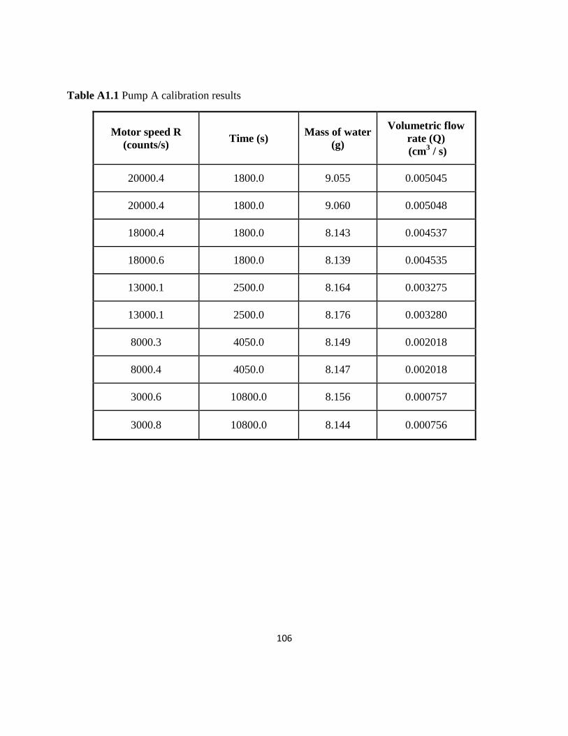
106
Table A1.1 Pump A calibration results
Motor speed R
(counts/s) Time (s)
Mass of water
(g)
Volumetric flow
rate (Q)
(cm3 / s)
20000.4 1800.0 9.055 0.005045
20000.4 1800.0 9.060 0.005048
18000.4 1800.0 8.143 0.004537
18000.6 1800.0 8.139 0.004535
13000.1 2500.0 8.164 0.003275
13000.1 2500.0 8.176 0.003280
8000.3 4050.0 8.149 0.002018
8000.4 4050.0 8.147 0.002018
3000.6 10800.0 8.156 0.000757
3000.8 10800.0 8.144 0.000756
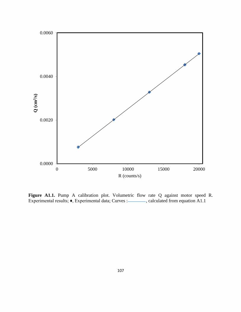
107
Figure A1.1. Pump A calibration plot. Volumetric flow rate Q against motor speed R.
Experimental results; ♦, Experimental data; Curves : , calculated from equation A1.1
0.0000
0.0020
0.0040
0.0060
0 5000 10000 15000 20000
Q (
cm3/s
)
R (counts/s)
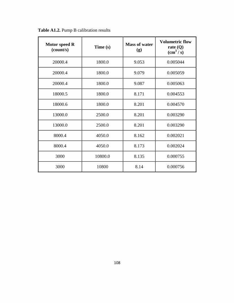
108
Table A1.2. Pump B calibration results
Motor speed R
(count/s) Time (s)
Mass of water
(g)
Volumetric flow
rate (Q)
(cm3 / s)
20000.4 1800.0 9.053 0.005044
20000.4 1800.0 9.079 0.005059
20000.4 1800.0 9.087 0.005063
18000.5 1800.0 8.171 0.004553
18000.6 1800.0 8.201 0.004570
13000.0 2500.0 8.201 0.003290
13000.0 2500.0 8.201 0.003290
8000.4 4050.0 8.162 0.002021
8000.4 4050.0 8.173 0.002024
3000 10800.0 8.135 0.000755
3000 10800 8.14 0.000756
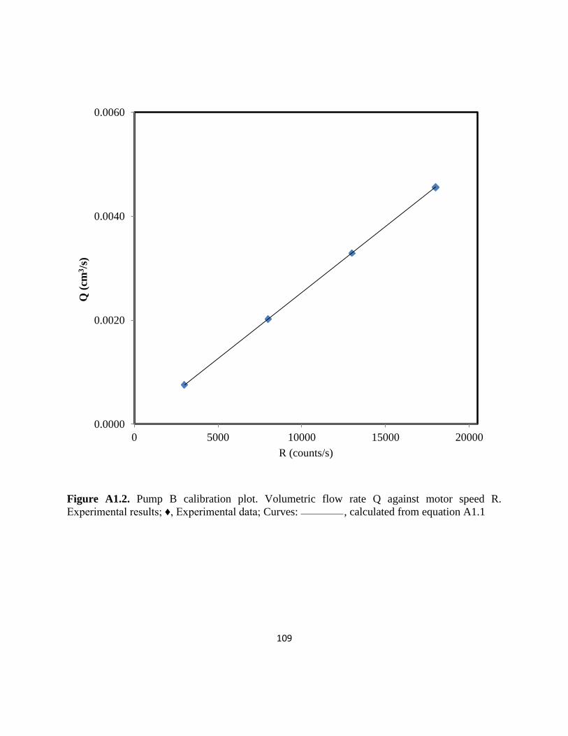
109
Figure A1.2. Pump B calibration plot. Volumetric flow rate Q against motor speed R.
Experimental results; ♦, Experimental data; Curves: , calculated from equation A1.1
0.0000
0.0020
0.0040
0.0060
0 5000 10000 15000 20000
Q (
cm3/s
)
R (counts/s)
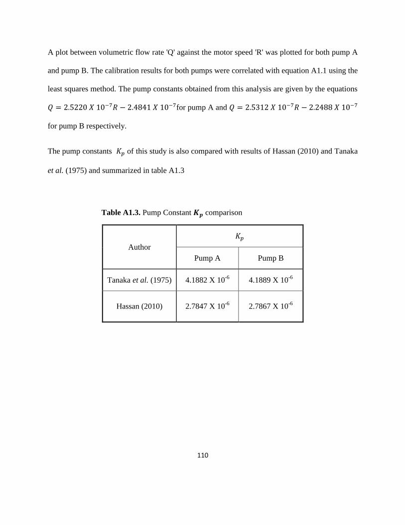
110
A plot between volumetric flow rate 'Q' against the motor speed 'R' was plotted for both pump A
and pump B. The calibration results for both pumps were correlated with equation A1.1 using the
least squares method. The pump constants obtained from this analysis are given by the equations
for pump A and
for pump B respectively.
The pump constants of this study is also compared with results of Hassan (2010) and Tanaka
et al. (1975) and summarized in table A1.3
Table A1.3. Pump Constant comparison
Author
Pump A Pump B
Tanaka et al. (1975) 4.1882 X 10⁻⁶
4.1889 X 10⁻⁶
Hassan (2010) 2.7847 X 10⁻⁶
2.7867 X 10⁻⁶
111
Appendix B
B1. Heats of mixing calculations for binary mixtures
B2. Weight corrections for buoyancy effect of air
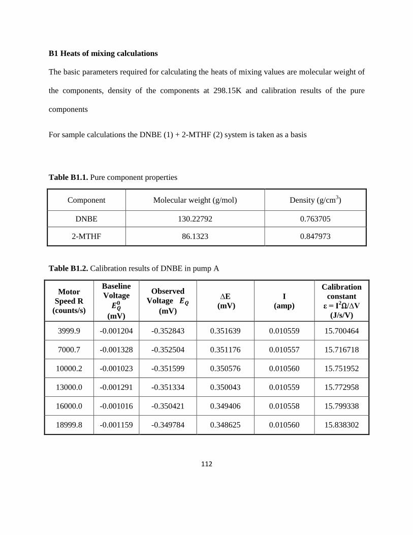
112
B1 Heats of mixing calculations
The basic parameters required for calculating the heats of mixing values are molecular weight of
the components, density of the components at 298.15K and calibration results of the pure
components
For sample calculations the DNBE (1) + 2-MTHF (2) system is taken as a basis
Table B1.1. Pure component properties
Component Molecular weight (g/mol) Density (g/cm3)
DNBE 130.22792 0.763705
2-MTHF 86.1323 0.847973
Table B1.2. Calibration results of DNBE in pump A
Motor
Speed R
(counts/s)
Baseline
Voltage
(mV)
Observed
Voltage
(mV)
∆E
(mV)
I
(amp)
Calibration
constant
ε = I2Ω/∆V
(J/s/V)
3999.9 -0.001204 -0.352843 0.351639 0.010559 15.700464
7000.7 -0.001328 -0.352504 0.351176 0.010557 15.716718
10000.2 -0.001023 -0.351599 0.350576 0.010560 15.751952
13000.0 -0.001291 -0.351334 0.350043 0.010559 15.772958
16000.0 -0.001016 -0.350421 0.349406 0.010558 15.799338
18999.8 -0.001159 -0.349784 0.348625 0.010560 15.838302
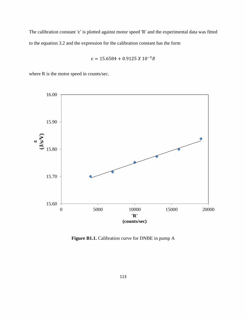
113
The calibration constant 'ɛ' is plotted against motor speed 'R' and the experimental data was fitted
to the equation 3.2 and the expression for the calibration constant has the form
ɛ
where R is the motor speed in counts/sec.
Figure B1.1. Calibration curve for DNBE in pump A
15.60
15.70
15.80
15.90
16.00
0 5000 10000 15000 20000
ε
(J/s
/V)
'R'
(counts/sec)
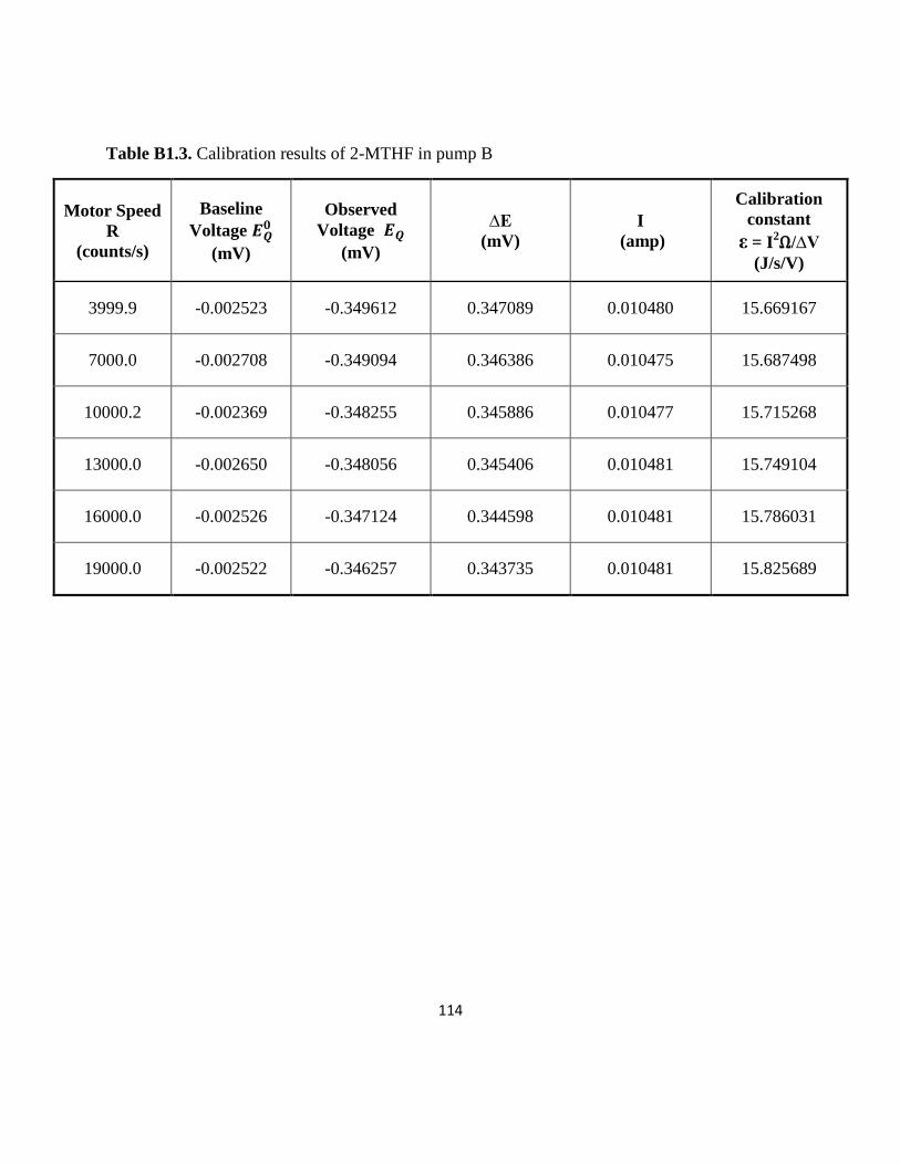
114
Table B1.3. Calibration results of 2-MTHF in pump B
Motor Speed
R
(counts/s)
Baseline
Voltage
(mV)
Observed
Voltage
(mV)
∆E
(mV)
I
(amp)
Calibration
constant
ε = I2Ω/∆V
(J/s/V)
3999.9 -0.002523 -0.349612 0.347089 0.010480 15.669167
7000.0 -0.002708 -0.349094 0.346386 0.010475 15.687498
10000.2 -0.002369 -0.348255 0.345886 0.010477 15.715268
13000.0 -0.002650 -0.348056 0.345406 0.010481 15.749104
16000.0 -0.002526 -0.347124 0.344598 0.010481 15.786031
19000.0 -0.002522 -0.346257 0.343735 0.010481 15.825689
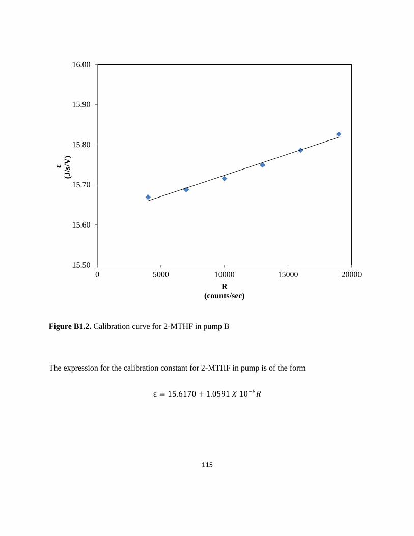
115
Figure B1.2. Calibration curve for 2-MTHF in pump B
The expression for the calibration constant for 2-MTHF in pump is of the form
ɛ
15.50
15.60
15.70
15.80
15.90
16.00
0 5000 10000 15000 20000
ε
(J/s
/V)
R
(counts/sec)
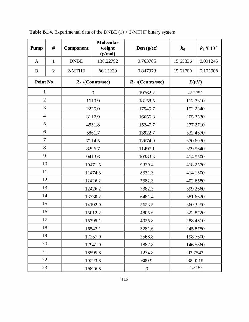
116
Table B1.4. Experimental data of the DNBE (1) + 2-MTHF binary system
Pump # Component
Molecular
weight
(g/mol)
Den (g/cc) k0 k1 X 10-4
A 1 DNBE 130.22792 0.763705 15.65836 0.091245
B 2 2-MTHF 86.13230 0.847973 15.61700 0.105908
Point No. RA /(Counts/sec) RB /(Counts/sec) E(μV)
1 0 19762.2 -2.2751
2 1610.9 18158.5 112.7610
3 2225.0 17545.7 152.2340
4 3117.9 16656.8 205.3530
5 4531.8 15247.7 277.2710
6 5861.7 13922.7 332.4670
7 7114.5 12674.0 370.6030
8 8296.7 11497.1 399.5640
9 9413.6 10383.3 414.5500
10 10471.5 9330.4 418.2570
11 11474.3 8331.3 414.1300
12 12426.2 7382.3 402.6580
13 12426.2 7382.3 399.2660
14 13330.2 6481.4 381.6620
15 14192.0 5623.5 360.3250
16 15012.2 4805.6 322.8720
17 15795.1 4025.8 288.4310
18 16542.1 3281.6 245.8750
19 17257.0 2568.8 198.7600
20 17941.0 1887.8 146.5860
21 18595.8 1234.8 92.7543
22 19223.8 609.9 38.0215
23 19826.8 0 -1.5154
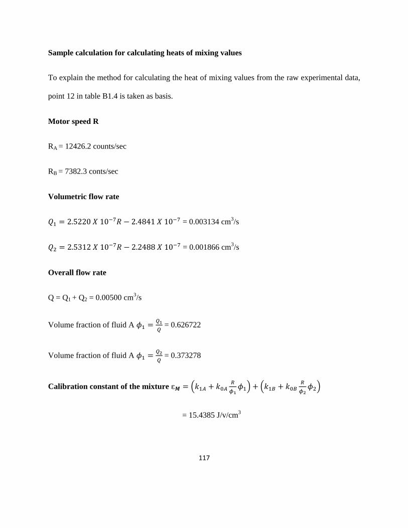
117
Sample calculation for calculating heats of mixing values
To explain the method for calculating the heat of mixing values from the raw experimental data,
point 12 in table B1.4 is taken as basis.
Motor speed R
RA = 12426.2 counts/sec
RB = 7382.3 conts/sec
Volumetric flow rate
= 0.003134 cm3/s
= 0.001866 cm3/s
Overall flow rate
Q = Q1 + Q2 = 0.00500 cm3/s
Volume fraction of fluid A
= 0.626722
Volume fraction of fluid A
= 0.373278
Calibration constant of the mixture ɛ (𝑘 𝑘
) (𝑘 𝑘
)
= 15.4385 J/v/cm3
118
Molar flow rate 'f'
where is the molar volume and it is calculated using the formula
Total molar flow rate, mol/s
Pure component baseline voltage
Mixture baseline voltage
⁄
=
Observed Voltage
Corrected Voltage
119
Mole fraction
Enthalpy
J/mol
Error Estimation
Calculation of error or uncertainty is an important aspect in this research work; it reflects the
accuracy of the measurements and methods. In this study the uncertainty of the data is calculated
using the error propagation method explained by Hassan (2010) thesis work.
The error propagation method is explained as follows
Let U be a dependent variable and it is a function of several measured variables,𝑢 , 𝑢 , etc.
𝑢 𝑢 (B1.1)
The error in the variable U is given by Bevington and Robinson (2003)
√(
)
(
)
(B1.2)
where is the standard deviation of the U dependent variable, ,
are the standard
deviation of the 𝑢 and 𝑢 variable respectively.
120
is the partial derivative of the variable U with respect to 𝑢
In this study a simpler approximation of the error propagation method is used.
Consider the variables 𝑢 and 𝑢 have errors 𝑢 and 𝑢 respectively, then uncertainties
in the dependent variable will be
i) For addition and subtraction: 𝑢 𝑢 or 𝑢 𝑢
√ 𝑢 𝑢
(B1.3)
ii) For multiplication and division: 𝑢 𝑢 or 𝑢 𝑢 ⁄
| | √(
)
(
)
(B1.4)
The uncertainties of the mole fraction and excess molar enthalpy were determined using the
equations B1.3 and B1.4.
Sample calculation
Molefraction uncertainty calculation
Error in volumetric flow rate
Volumetric flow rate Qi
Error
121
| |√(
𝑚 )
(
)
( 𝑡𝑖𝑚 𝑡𝑖𝑚
)
where, m = 9.055g, m = ±0.001g, ρwater = 0.99705 g/cm3, ρ = ± 0.00001 g/cm
3, time =
1800 s, time = ± 0.1 s. Then the error in the flow rate corresponding to cm3/s
is cm3/s.
Error in counter reading
RA = ± 0.5 counts/s and RB = ± 0.5 counts/s
Error in molar volume
Molar volume
|
| √(
)
(
)
where, M1 = 170.5212 g/mol, M1 = 0; g/cm3, ρ = ± 0.0.00001g/cm
3. Then
the error in the molar volume corresponding to 170.512 g/cm
3 is
= ± 0.0022
cm3/mol.
In the same way 101.5743 g/cm
3 is
= ± 0.0012 cm3/mol.
122
Error in molar flow rate
Molar flow rate
| | √(
)
(
)
when, cm3/s and mol/s,.the error,
.mol/s
when, cm3/s and mol/s, the error,
mol/s
Therefore the error in the total molar flow rate f is
√
mol/s
Molefraction
Error in molefraction is calculated using the equation
| | √(
)
(
)
so for the error in molefraction is
123
Error in excess molar enthalpy
Excess molar enthalpy is given by the formula
ɛ
where,
ɛ ɛ ɛ = A + B, where ɛ and ɛ and error in A and B can be
calculated using the equation
| | √( ɛ ɛ
)
(
)
and
| | √( ɛ ɛ
)
(
)
The error ɛ can be calculated by the relation
ɛ √
The uncertainty in the calibration constants of the pure components are estimated to be
ɛ J/s/V and ɛ J/s/V
Using the above values the error in the calibration constant for the mixture for ɛ value of
15.8345 J/v/cm3, is found to be ɛ = 0.00002398 J/V/cm
3.
124
Assuming the uncertainty in the voltage measurement to be = ± 0.01 μV, the uncertainty
in the excess molar enthalpy value of = 174.26 J/mol is calculated using the equation
|
| √( ɛ
ɛ )
(
)
(
)
(
)
= ± 0.04 J/mol.
Heat of mixing calculations for pseudo-binary mixture is same as the pure binary mixture; in
pseudo-binary system the component 2 is prepared from component 2 and component 3 of the
respective ternary system. The molecular weight and molefraction of the prepared pseudo binary
mixture is calculated after correcting the weights for buoyancy effect of air. The density of the
pseudo-binary mixture at 2698.15K was measured using the densitometer.
Details for calculating the molefraction of the pseudo-binary mixture and for correcting weights
to eliminate the buoyancy effect of air was explained in detail in appendix B2.
125
B2 Weight corrections for buoyancy effect of air
Hassan, 2010 in his thesis explained (Bauer, 1959) method for correcting the weights to elimante
the buoyancy effect of air. The formula is of the form
𝑚 𝑚
(
)
(
) (B2.1)
where, 𝑚 , corrected mass of the sample, density of the weighed sample, 𝑚 measured
weight of the sample, density of air, density of brass (built in weights of the balance used
and has a value of 8.4 g/cm3)
Density of air calculation
In general, most weight measurements are made in an environment surrounded by air, the density
of air acts as a buoyancy force on the weighed sample. The density of the air needs to be
calculated to eliminate the buoyancy effect of air. Bauer, 1959 equation can be used to calculate
the density of air
𝑚 ⁄ ⁄
(B2.2)
where, P is the atmospheric pressure in mmHg, RH the relative humidity of the surrounding in %,
and t is the room temperature in C, and is the vapor pressure of water at room
temperature and it is calculated using Antoine equation
𝑙𝑜 𝑚𝑚 ⁄
𝑡
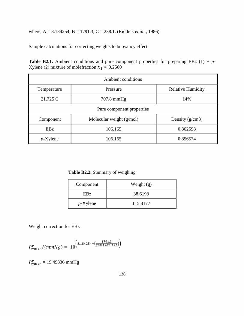
126
where, A = 8.184254, B = 1791.3, C = 238.1. (Riddick et al.., 1986)
Sample calculations for correcting weights to buoyancy effect
Table B2.1. Ambient conditions and pure component properties for preparing EBz (1) + p-
Xylene (2) mixture of molefraction 0.2500
Ambient conditions
Temperature Pressure Relative Humidity
21.725 C 707.8 mmHg 14%
Pure component properties
Component Molecular weight (g/mol) Density (g/cm3)
EBz 106.165 0.862598
p-Xylene 106.165 0.856574
Table B2.2. Summary of weighing
Component Weight (g)
EBz 38.6193
p-Xylene 115.8177
Weight correction for EBz
𝑚𝑚 ⁄
( (
))
= 19.49836 mmHg
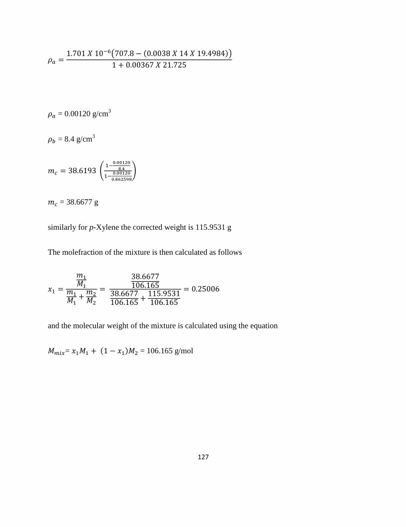
127
( )
= 0.00120 g/cm3
= 8.4 g/cm3
𝑚 (
)
𝑚 = 38.6677 g
similarly for p-Xylene the corrected weight is 115.9531 g
The molefraction of the mixture is then calculated as follows
𝑚
𝑚
𝑚
and the molecular weight of the mixture is calculated using the equation
= = 106.165 g/mol
128
Appendix C
C1. Statistics of data Correlation
C2. Liebermann-Fried model representation of ternary systems
129
C1 Statistics of data correlation
The experimental excess molar enthalpy data was fitted to empirical equations and solution
theory model by means of unweighted least square method. This study continued the method
used by (Hassan, 2010) for performing the statistical tests. The Marquardt method (Levenberg-
Marquardt algorithm; (Marquardt, 1963) was used for finding the best Redlich-Kister fit
parameters and Microsoft excel solver function was used to fit the Liebermann-Fried model and
the Tsao and Smith equation. The solver function uses the Generalized Reduced Gradient
(GRG2) Algorithm (Lasdon et al.., 1978) for solving nonlinear problems. The standard error was
used as the objective function for both methods and it is expressed as
𝑠 √∑ 𝑝 𝑟𝑖𝑚 𝑛𝑡 𝑙 𝑣 𝑙𝑢 𝑠 𝑙 𝑢𝑙 𝑡 𝑣 𝑙𝑢 𝑠
𝑛 𝑝
where, n is the number of data points, and p is the number of adjustable parameters of the model.
The parameters are selected based on the minimization of the objective function. The total
numbers of parameters representing the best fit of the experimental values are chosen by means
of F - statistical test.
F-statistical test
When experimental data are fitted to a model, a model with large number of parameters will
have a low standard error than a model with less number of parameters. Quite often it is assumed
that a model with large number of parameter provides the best fit of the experimental data, but it
does not always represent the statistically better fit than a model with less number of parameters.
In this case, statistical tests help to choose the model which most accurately represents the
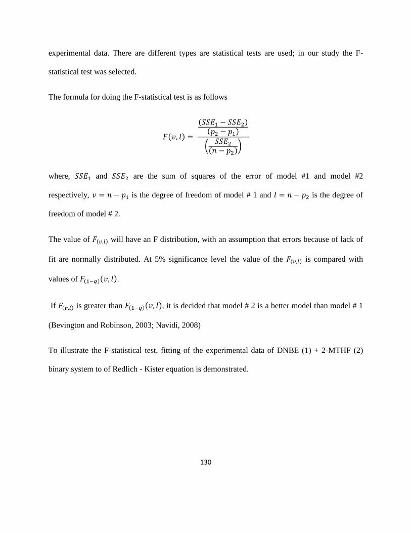
130
experimental data. There are different types are statistical tests are used; in our study the F-
statistical test was selected.
The formula for doing the F-statistical test is as follows
𝑣 𝑙
𝑝 𝑝
(
𝑛 𝑝 )
where, and are the sum of squares of the error of model #1 and model #2
respectively, 𝑣 𝑛 𝑝 is the degree of freedom of model # 1 and 𝑙 𝑛 𝑝 is the degree of
freedom of model # 2.
The value of will have an F distribution, with an assumption that errors because of lack of
fit are normally distributed. At 5% significance level the value of the is compared with
values of 𝑣 𝑙 .
If is greater than 𝑣 𝑙 , it is decided that model # 2 is a better model than model # 1
(Bevington and Robinson, 2003; Navidi, 2008)
To illustrate the F-statistical test, fitting of the experimental data of DNBE (1) + 2-MTHF (2)
binary system to of Redlich - Kister equation is demonstrated.
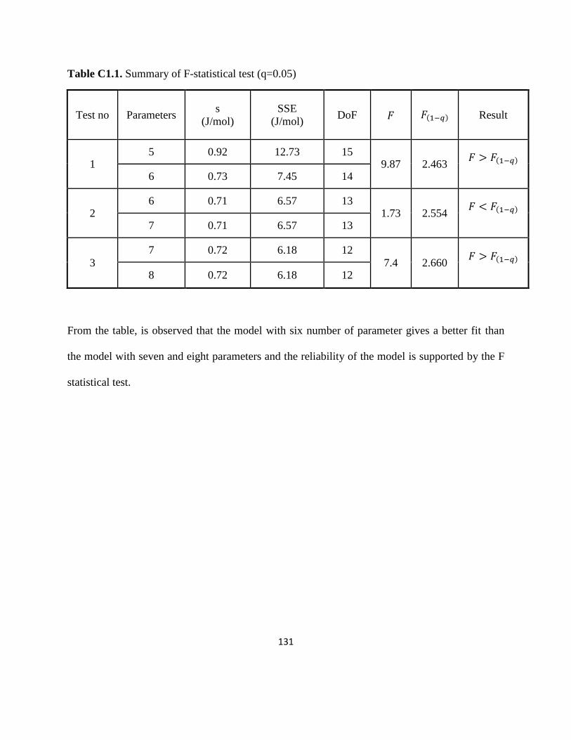
131
Table C1.1. Summary of F-statistical test (q=0.05)
Test no Parameters s
(J/mol)
SSE
(J/mol) DoF Result
1 5 0.92 12.73 15
9.87 2.463
6 0.73 7.45 14
2 6 0.71 6.57 13
1.73 2.554
7 0.71 6.57 13
3
7 0.72 6.18 12
7.4 2.660
8 0.72 6.18 12
From the table, is observed that the model with six number of parameter gives a better fit than
the model with seven and eight parameters and the reliability of the model is supported by the F
statistical test.
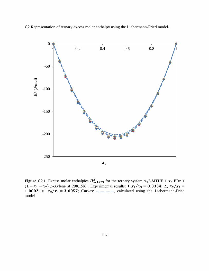
132
C2 Representation of ternary excess molar enthalpy using the Liebermann-Fried model.
Figure C2.1. Excess molar enthalpies for the ternary system 2-MTHF + EBz +
p-Xylene at 298.15K . Experimental results: ♦ ⁄ : , ⁄ ; , ⁄ ; Curves: , calculated using the Liebermann-Fried
model
-250
-200
-150
-100
-50
0
0 0.2 0.4 0.6 0.8 1
HE (
J/m
ol)
𝑥1
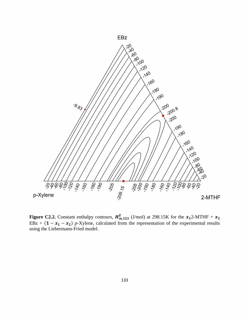
133
Figure C2.2. Constant enthalpy contours, (J/mol) at 298.15K for the 2-MTHF +
EBz + p-Xylene, calculated from the representation of the experimental results
using the Liebermann-Fried model.
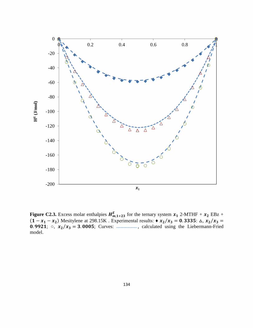
134
Figure C2.3. Excess molar enthalpies for the ternary system 2-MTHF + EBz +
Mesitylene at 298.15K . Experimental results: ♦ ⁄ : , ⁄ ; , ⁄ ; Curves: , calculated using the Liebermann-Fried
model.
-200
-180
-160
-140
-120
-100
-80
-60
-40
-20
0
0 0.2 0.4 0.6 0.8 1
HE (
J/m
ol)
𝑥1
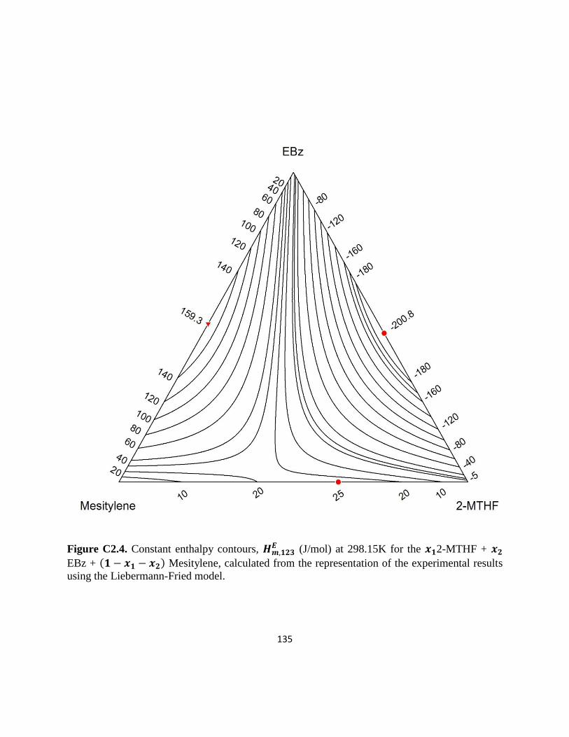
135
Figure C2.4. Constant enthalpy contours, (J/mol) at 298.15K for the 2-MTHF +
EBz + Mesitylene, calculated from the representation of the experimental results
using the Liebermann-Fried model.
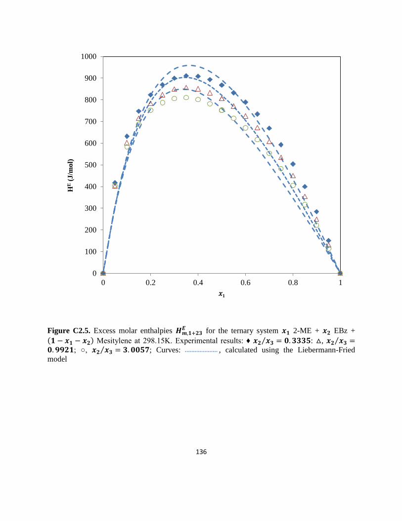
136
Figure C2.5. Excess molar enthalpies for the ternary system 2-ME + EBz +
Mesitylene at 298.15K. Experimental results: ♦ ⁄ : , ⁄ ; , ⁄ ; Curves: , calculated using the Liebermann-Fried
model
0
100
200
300
400
500
600
700
800
900
1000
0 0.2 0.4 0.6 0.8 1
HE (
J/m
ol)
𝑥1
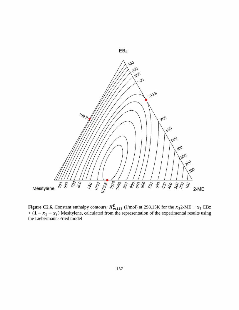
137
Figure C2.6. Constant enthalpy contours, (J/mol) at 298.15K for the 2-ME + EBz
+ Mesitylene, calculated from the representation of the experimental results using
the Liebermann-Fried model
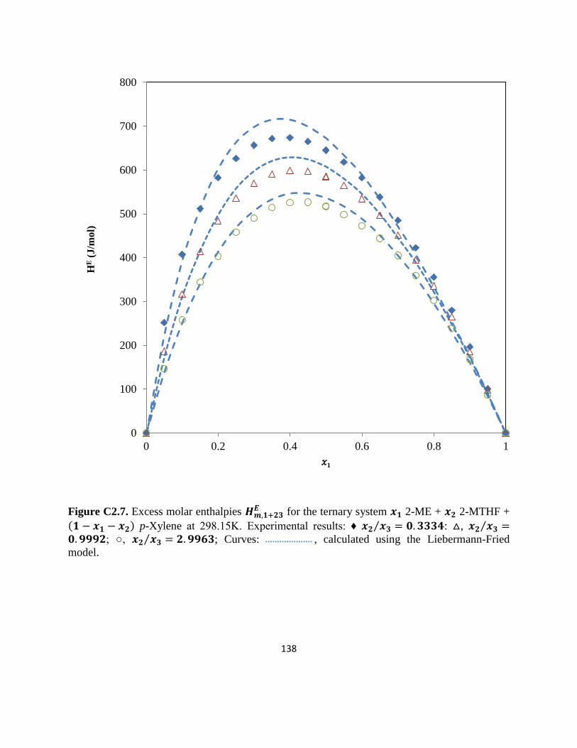
138
Figure C2.7. Excess molar enthalpies for the ternary system 2-ME + 2-MTHF +
p-Xylene at 298.15K. Experimental results: ♦ ⁄ : , ⁄ ; , ⁄ ; Curves: , calculated using the Liebermann-Fried
model.
0
100
200
300
400
500
600
700
800
0 0.2 0.4 0.6 0.8 1
HE (
J/m
ol)
𝑥1
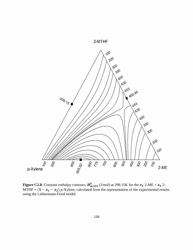
139
Figure C2.8. Constant enthalpy contours, (J/mol) at 298.15K for the 2-ME + 2-
MTHF + p-Xylene, calculated from the representation of the experimental results
using the Liebermann-Fried model.
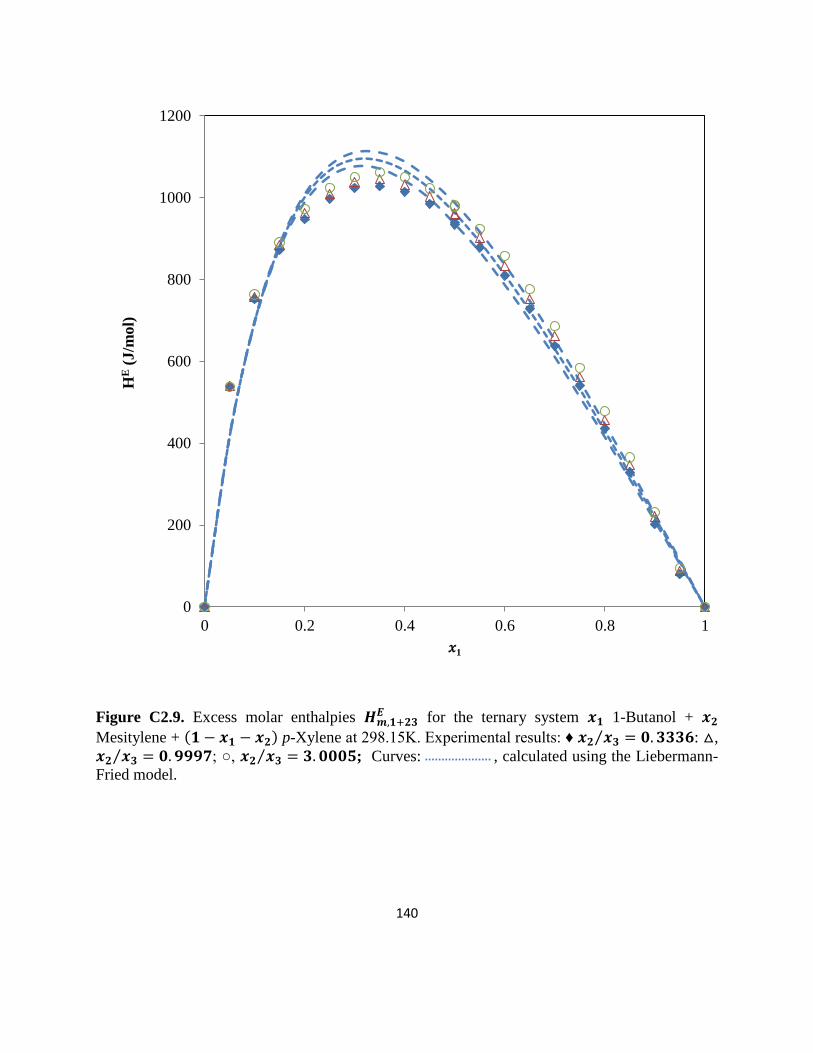
140
Figure C2.9. Excess molar enthalpies for the ternary system 1-Butanol +
Mesitylene + p-Xylene at 298.15K. Experimental results: ♦ ⁄ : ,
⁄ ; , ⁄ ; Curves: , calculated using the Liebermann-
Fried model.
0
200
400
600
800
1000
1200
0 0.2 0.4 0.6 0.8 1
HE (
J/m
ol)
𝑥1
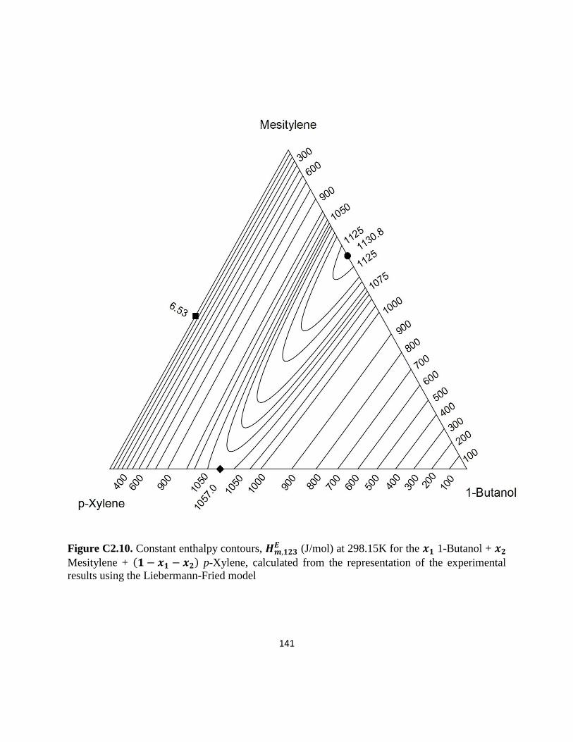
141
Figure C2.10. Constant enthalpy contours, (J/mol) at 298.15K for the 1-Butanol +
Mesitylene + p-Xylene, calculated from the representation of the experimental
results using the Liebermann-Fried model
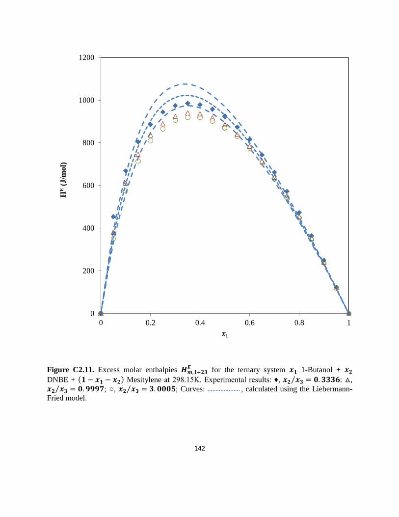
142
Figure C2.11. Excess molar enthalpies for the ternary system 1-Butanol +
DNBE + Mesitylene at 298.15K. Experimental results: ♦, ⁄ : ,
⁄ ; , ⁄ ; Curves: , calculated using the Liebermann-
Fried model.
0
200
400
600
800
1000
1200
0 0.2 0.4 0.6 0.8 1
HE (
J/m
ol)
𝑥1
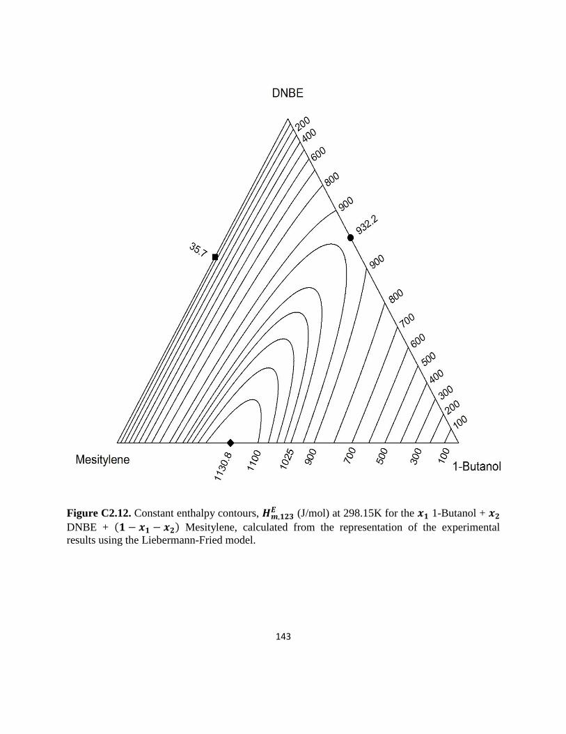
143
Figure C2.12. Constant enthalpy contours, (J/mol) at 298.15K for the 1-Butanol +
DNBE + Mesitylene, calculated from the representation of the experimental
results using the Liebermann-Fried model.
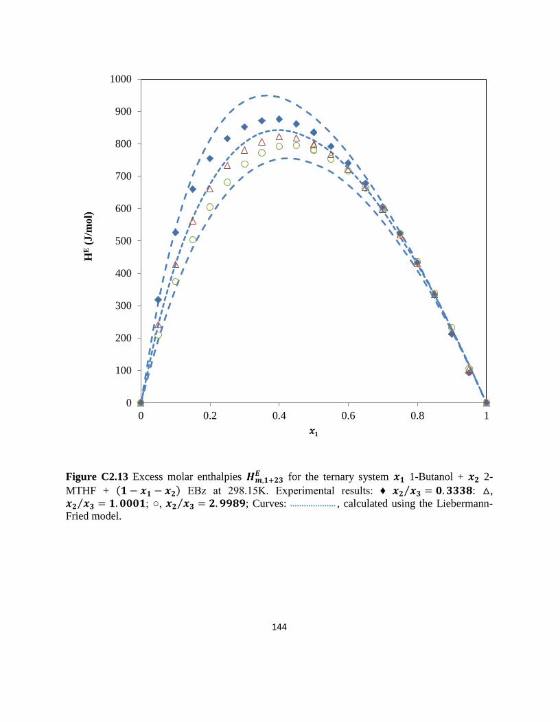
144
Figure C2.13 Excess molar enthalpies for the ternary system 1-Butanol + 2-
MTHF + EBz at 298.15K. Experimental results: ♦ ⁄ : ,
⁄ ; , ⁄ ; Curves: , calculated using the Liebermann-
Fried model.
0
100
200
300
400
500
600
700
800
900
1000
0 0.2 0.4 0.6 0.8 1
HE (
J/m
ol)
𝑥1
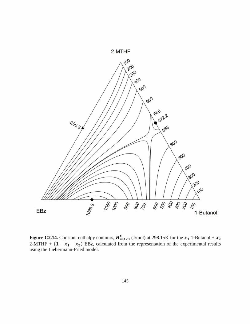
145
Figure C2.14. Constant enthalpy contours, (J/mol) at 298.15K for the 1-Butanol +
2-MTHF + EBz, calculated from the representation of the experimental results
using the Liebermann-Fried model.
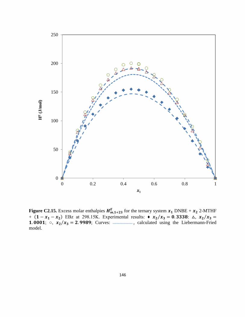
146
Figure C2.15. Excess molar enthalpies for the ternary system DNBE + 2-MTHF
+ EBz at 298.15K. Experimental results: ♦ ⁄ : , ⁄ ; , ⁄ ; Curves: , calculated using the Liebermann-Fried
model.
0
50
100
150
200
250
0 0.2 0.4 0.6 0.8 1
HE (
J/m
ol)
𝑥1
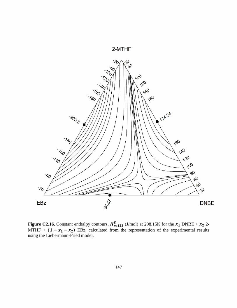
147
Figure C2.16. Constant enthalpy contours, (J/mol) at 298.15K for the DNBE + 2-
MTHF + EBz, calculated from the representation of the experimental results
using the Liebermann-Fried model.
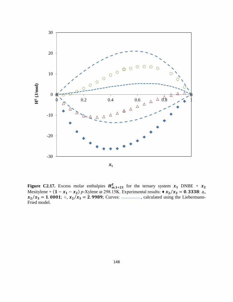
148
Figure C2.17. Excess molar enthalpies for the ternary system DNBE +
Mesitylene + p-Xylene at 298.15K. Experimental results: ♦ ⁄ : ,
⁄ ; , ⁄ ; Curves: , calculated using the Liebermann-
Fried model.
-30
-20
-10
0
10
20
30
0 0.2 0.4 0.6 0.8 1
HE (
J/m
ol)
𝑥1
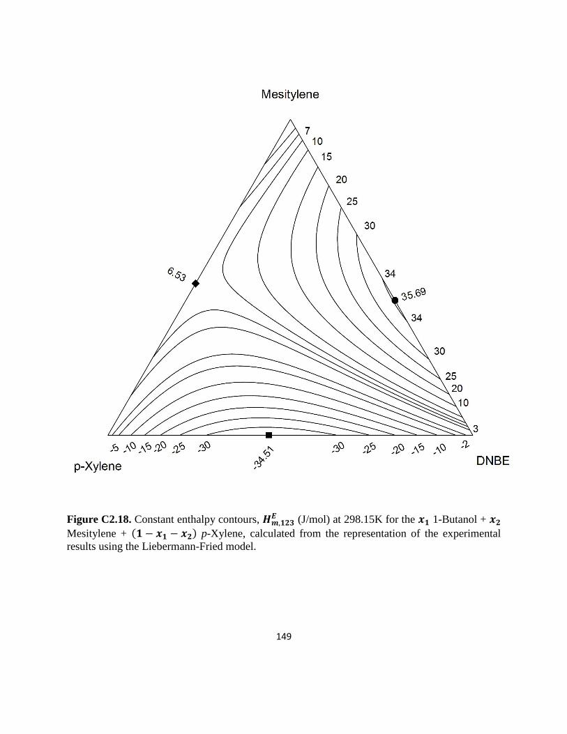
149
Figure C2.18. Constant enthalpy contours, (J/mol) at 298.15K for the 1-Butanol +
Mesitylene + p-Xylene, calculated from the representation of the experimental
results using the Liebermann-Fried model.
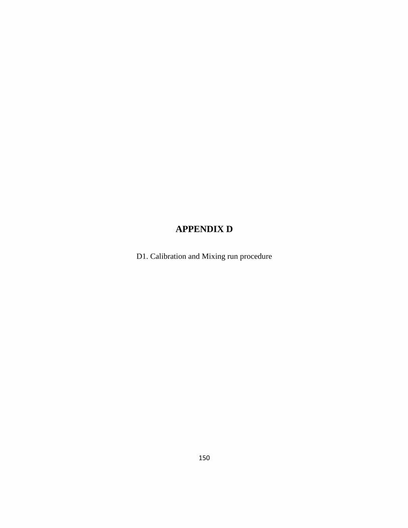
150
APPENDIX D
D1. Calibration and Mixing run procedure

151
D.1 Calibration and Mixing run procedure
The following steps should be carried out first before starting any mixing or calibration run,
The water bath enclosing the calorimeter should be maintained at 25 ± 0.005°C for at
least 24 hours
Both syringe A and syringe B are first cleaned with ethanol and then with acetone and
finally purged with nitrogen for complete cleaning.
The chemicals species A and species B should be dewatered with molecular sieves for at
least 24 hours and then degassed by means of a vacuum pump.
(The molecular sieves used for dewatering must be baked in an oven at temperatures higher than
100°C for at least 24 hours)
Calibration run procedure
Considering species A is calibrated in pump A
1) Syringe A is charged with species A and the flow control valve (figure D1.1) is connected to
the syringe A
2) One end of the flow control valve is connected to the reservoir flask and the other end of the
valve is connected to the Teflon tube tagged as pump A leading to the calorimeter
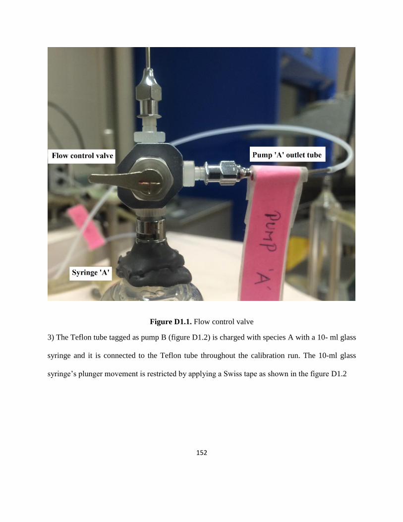
152
Figure D1.1. Flow control valve
3) The Teflon tube tagged as pump B (figure D1.2) is charged with species A with a 10- ml glass
syringe and it is connected to the Teflon tube throughout the calibration run. The 10-ml glass
syringe’s plunger movement is restricted by applying a Swiss tape as shown in the figure D1.2
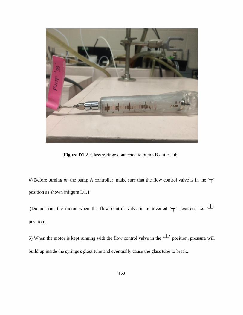
153
Figure D1.2. Glass syringe connected to pump B outlet tube
4) Before turning on the pump A controller, make sure that the flow control valve is in the ‘’
position as shown infigure D1.1
(Do not run the motor when the flow control valve is in inverted ‘’ position, i.e. ‘’
position).
5) When the motor is kept running with the flow control valve in the ‘’ position, pressure will
build up inside the syringe's glass tube and eventually cause the glass tube to break.
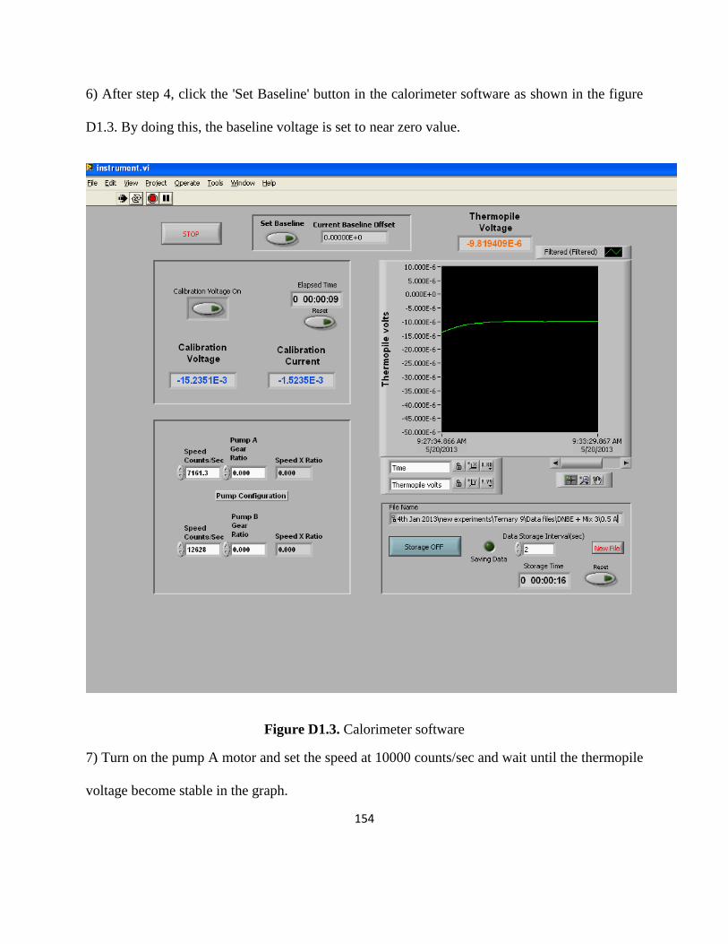
154
6) After step 4, click the 'Set Baseline' button in the calorimeter software as shown in the figure
D1.3. By doing this, the baseline voltage is set to near zero value.
Figure D1.3. Calorimeter software
7) Turn on the pump A motor and set the speed at 10000 counts/sec and wait until the thermopile
voltage become stable in the graph.
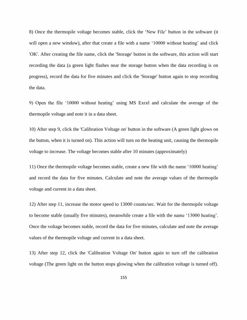
155
8) Once the thermopile voltage becomes stable, click the ‘New File’ button in the software (it
will open a new window), after that create a file with a name ‘10000 without heating’ and click
'OK'. After creating the file name, click the 'Storage' button in the software, this action will start
recording the data (a green light flashes near the storage button when the data recording is on
progress), record the data for five minutes and click the 'Storage' button again to stop recording
the data.
9) Open the file ‘10000 without heating’ using MS Excel and calculate the average of the
thermopile voltage and note it in a data sheet.
10) After step 9, click the 'Calibration Voltage on' button in the software (A green light glows on
the button, when it is turned on). This action will turn on the heating unit, causing the thermopile
voltage to increase. The voltage becomes stable after 10 minutes (approximately)
11) Once the thermopile voltage becomes stable, create a new file with the name ‘10000 heating’
and record the data for five minutes. Calculate and note the average values of the thermopile
voltage and current in a data sheet.
12) After step 11, increase the motor speed to 13000 counts/sec. Wait for the thermopile voltage
to become stable (usually five minutes), meanwhile create a file with the name ‘13000 heating’.
Once the voltage becomes stable, record the data for five minutes, calculate and note the average
values of the thermopile voltage and current in a data sheet.
13) After step 12, click the 'Calibration Voltage On' button again to turn off the calibration
voltage (The green light on the button stops glowing when the calibration voltage is turned off).
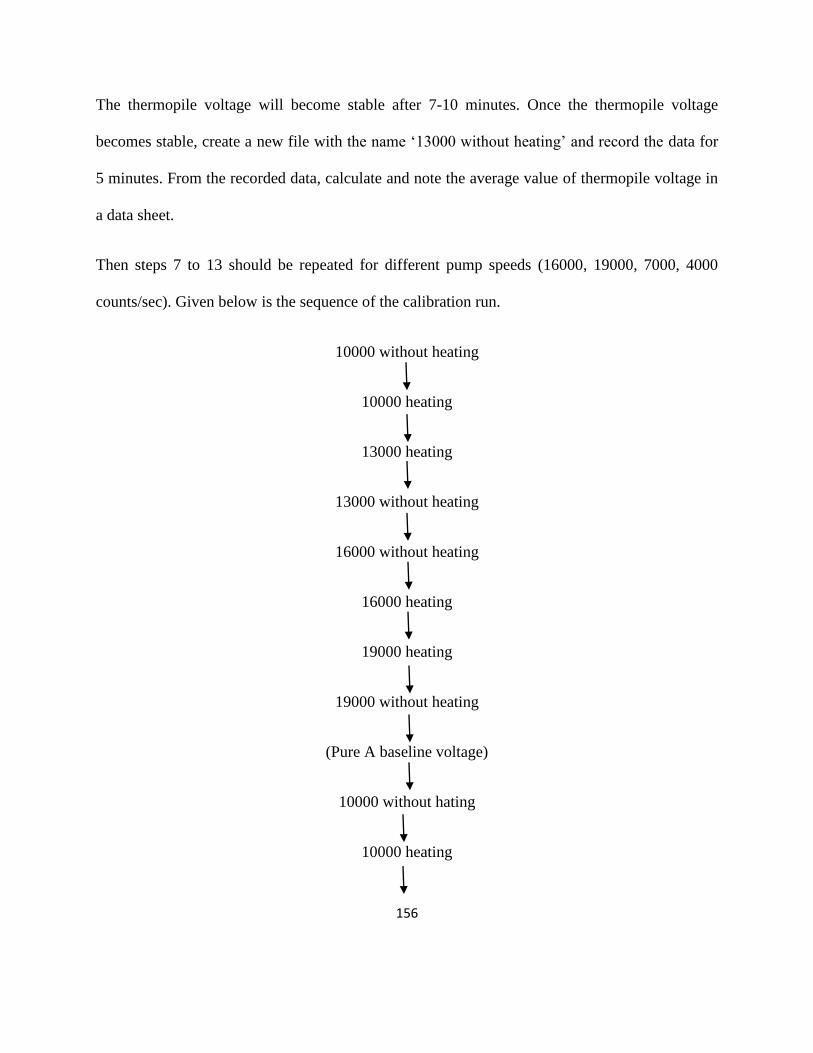
156
The thermopile voltage will become stable after 7-10 minutes. Once the thermopile voltage
becomes stable, create a new file with the name ‘13000 without heating’ and record the data for
5 minutes. From the recorded data, calculate and note the average value of thermopile voltage in
a data sheet.
Then steps 7 to 13 should be repeated for different pump speeds (16000, 19000, 7000, 4000
counts/sec). Given below is the sequence of the calibration run.
10000 without heating
10000 heating
13000 heating
13000 without heating
16000 without heating
16000 heating
19000 heating
19000 without heating
(Pure A baseline voltage)
10000 without hating
10000 heating
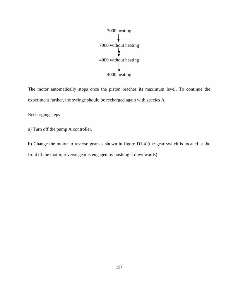
157
7000 heating
7000 without heating
4000 without heating
4000 heating
The motor automatically stops once the piston reaches its maximum level. To continue the
experiment further, the syringe should be recharged again with species A.
Recharging steps
a) Turn off the pump A controller.
b) Change the motor to reverse gear as shown in figure D1.4 (the gear switch is located at the
front of the motor, reverse gear is engaged by pushing it downwards)
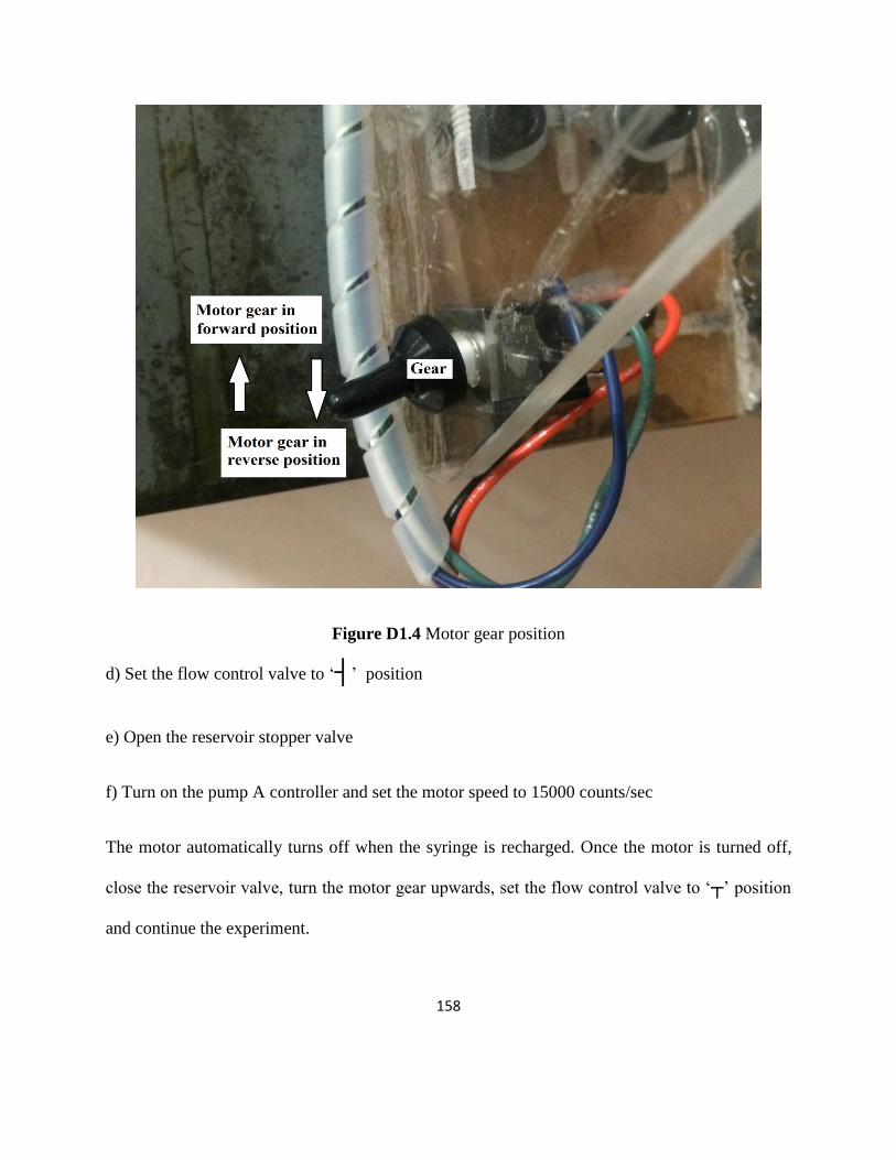
158
Figure D1.4 Motor gear position
d) Set the flow control valve to ‘’ position
e) Open the reservoir stopper valve
f) Turn on the pump A controller and set the motor speed to 15000 counts/sec
The motor automatically turns off when the syringe is recharged. Once the motor is turned off,
close the reservoir valve, turn the motor gear upwards, set the flow control valve to ‘’ position
and continue the experiment.
159
The calibration procedure for the pump B is similar to that of pump A with few changes and they
are
i) Species B is charged in syringe B
ii) Species B is filled in the Teflon tube marked as Pump A.
Mixing run procedure
Mixing run should be carried out after finishing the calibration run for species A in pump A and
species B in pump B respectively.
Before starting the mixing run 'motor speed table' should be generated. (An excel template is
available in the lab computer to calculate the motor speed)
After creating the motor speed table, following steps should be followed
1) The flow control valves of syringe and syringe B should be in ‘’ position
2) The motor gears for both pump A and pump B should be in upward direction.
3) The pump controllers are turned on and the mixing run is carried out in the following order
The 1-Butanol (1) + p-Xylene (2) mixing run is taken as the basis for explaining the mixing run
procedure.
Table D1.1 illustrates the 1-Butanol (1) + p-Xylene (2) mixing run. The mixing run has two
parts, one that starts with equimolar molefraction and ends with and the
160
other part starts again with equimolar molefraction and ends with . Following
flow chart illustrates the above explained steps.
First
Followed by to
Then is repeated
Followed by to
a) The mixing run is started with the pump A speed 8447.2 counts/sec and pump B speed
11346.9 counts/sec, which brings the mole fraction of the mixture . After the start,
proper mixing of the components takes place in 20 minutes, a stable thermopile voltage can be
seen in the screen once the mixing takes place properly. (During the first 15 minutes of the
mixing run, a continuous stream of air bubbles comes out of the exit tube and this occurrence of
bubbles is normal for a mixing run)
b) Once the thermopile voltage becomes stable, create a ‘new file’ with the name ‘0.5 + 0.5 B’
and record the data for five minutes. Here ‘ ’ represents pump fluid 1-Butanol and ‘B’
represents pump B fluid p-Xylene.
c) Stop recording the data after five minutes, open the file where the data has been recorded,
calculate the average value and record the average in a data sheet.
d) Change the motor speed of pump A and B for the molefraction, in this case 7491.7
counts/sec and 12298.9 counts/sec respectively.
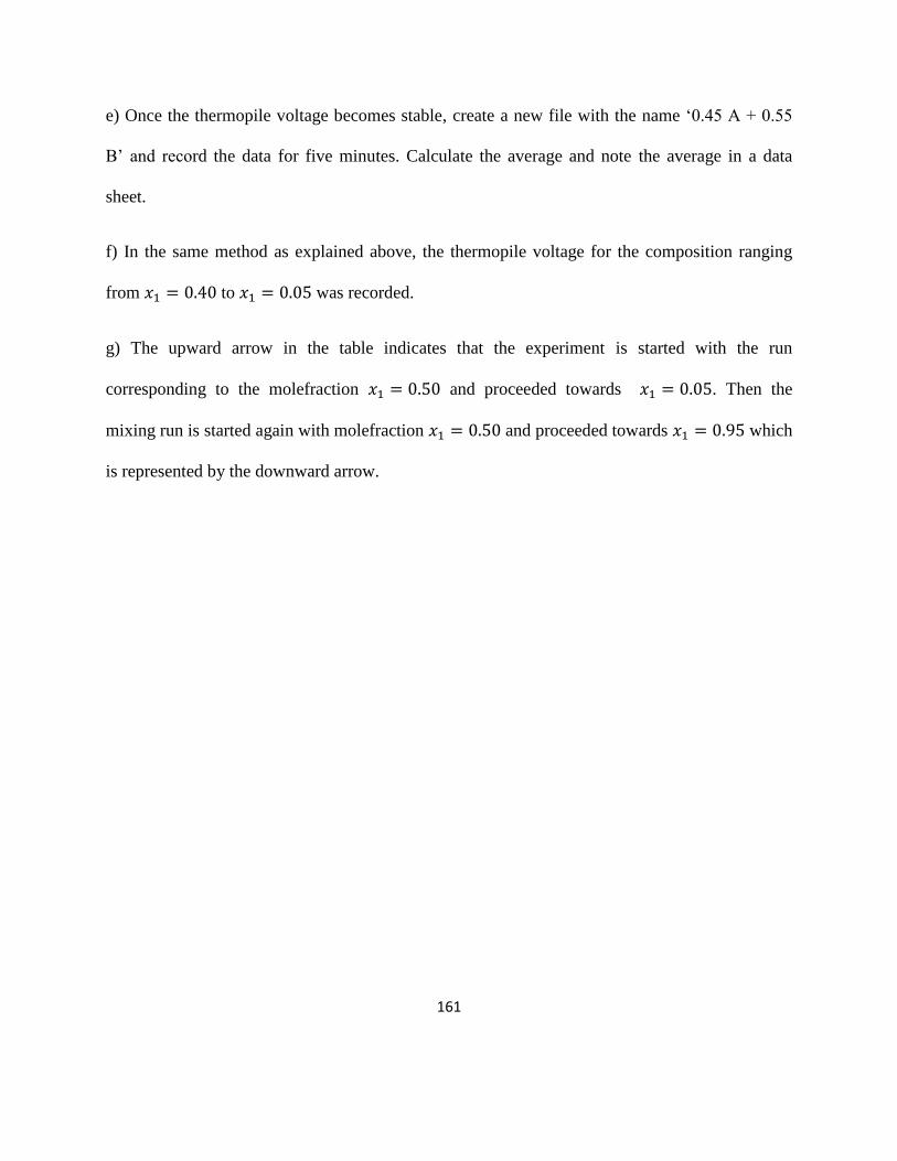
161
e) Once the thermopile voltage becomes stable, create a new file with the name ‘0.45 + 0.55
B’ and record the data for five minutes. Calculate the average and note the average in a data
sheet.
f) In the same method as explained above, the thermopile voltage for the composition ranging
from to was recorded.
g) The upward arrow in the table indicates that the experiment is started with the run
corresponding to the molefraction and proceeded towards . Then the
mixing run is started again with molefraction and proceeded towards which
is represented by the downward arrow.
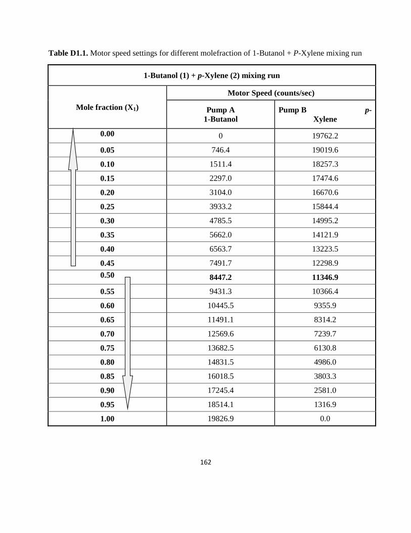
162
Table D1.1. Motor speed settings for different molefraction of 1-Butanol + P-Xylene mixing run
1-Butanol (1) + p-Xylene (2) mixing run
Mole fraction (X1)
Motor Speed (counts/sec)
Pump A
1-Butanol
Pump B p-
Xylene
0.00 0 19762.2
0.05 746.4 19019.6
0.10 1511.4 18257.3
0.15 2297.0 17474.6
0.20 3104.0 16670.6
0.25 3933.2 15844.4
0.30 4785.5 14995.2
0.35 5662.0 14121.9
0.40 6563.7 13223.5
0.45 7491.7 12298.9
0.50 8447.2 11346.9
0.55 9431.3 10366.4
0.60 10445.5 9355.9
0.65 11491.1 8314.2
0.70 12569.6 7239.7
0.75 13682.5 6130.8
0.80 14831.5 4986.0
0.85 16018.5 3803.3
0.90 17245.4 2581.0
0.95 18514.1 1316.9
1.00 19826.9 0.0
163
If bubbles come out of the exit tube during the mixing run, it will cause the thermopile voltage to
fluctuate abnormally. The fluctuations can be seen in the graph on the screen. In that case, data
recording should be stopped and disregarded for that particular run.
Once the air bubbles stops appearing at the exit tube, wait for a stable thermopile voltage and
start recording the data again for that specific run.
(Bubble formation during the mixing run can be avoided by proper degassing of the pure
component species)
4/17/2014 Gmail - Permission request
https://mail.google.com/mail/u/1/?ui=2&ik=953dd7ea0b&view=pt&q=hasan.nazmul%40usask.ca&qs=true&search=query&th=14258f211dae58fd&siml=14258f21… 1/2
Permission request 3 messages
manju nathan <[email protected]>
manju nathan <[email protected]> Thu, Nov 14, 2013 at 5:28 PM
To: Nazmul Hasan <[email protected]>
Dear Nazmul,
How are you and how is your job? I hope you are doing well out there!
I am writing my thesis now, since my research is continuation of your work, I want to use some of the materials
from your dissertation and I am requesting your permission to use them in my thesis work.
The details of the materials which I want to use from your thesis are figure 3.1, 3.2, 3.3 and 3.4 from chapter 3.
Thank you
Regards,
Manju.
Hasan, S M Nazmul <[email protected]> Thu, Nov 14, 2013 at 5:55 PM
To: manju nathan <[email protected]>
Hi Manju,
Congratulation on finishing your experiments. Yes, sure you can use those figures. How is everything going? How
is Dr. Peng? Does he have any new student?
Good luck.
Regards,
Nazmul Hasan
[Quoted text hi dden]
manju nathan <[email protected]> Fri, Nov 15, 2013 at 11:03 AM
To: "Hasan, S M Nazmul" <[email protected]>
Thanks Nazmul,
Dr. Peng is doing great, he is quite busy with his teaching and administration works, yes he took a new Ph.D
student she is from Iran.
and thanks for the wishes Nazmul :)
Manju.
[Quoted text hi dden]
--
Manjunathan,
M.Sc Student
Dept.Of.Chemical Engineering,
4/17/2014 Gmail - Permission request
https://mail.google.com/mail/u/1/?ui=2&ik=953dd7ea0b&view=pt&q=hasan.nazmul%40usask.ca&qs=true&search=query&th=14258f211dae58fd&siml=14258f21… 2/2
University Of Saskatchewan.
Related Documents


