Mean stress effect correction using constant stress ratio S–N curves

1

Mean Stress Effect Correction using Constant Stress Ratio S-N Curves

Adam NIESŁONYa,*, Michał BÖHMa

a Opole University of Technology, Faculty of Mechanical Engineering,

Department of Mechanics and Machine Design, ul. Mikołajczyka 5, 45-271 Opole, Poland

* Corresponding author. Tel.: +48 77 400 83 99; fax: +48 77 449 99 06.

E-mail address: [email protected] (A. Niesłony).

Abstract

This paper presents an stress based approach to take into account the influence of the mean

stress value on fatigue strength of constructional materials. Elaborated model uses two S-N

curves, i.e. for alternating stress (R = 1) and another one obtained under stress ratio R 1,

for calibrating the equations of boundary condition. Two particular equations for the

coefficient of intensification in stress transformations were proposed. The main advantage of

the proposed solution is that the mean stress effect correction depends on number of cycles to

failure, what corresponds to observed changes in experimental results presented in the

literature. Proposed relations were compared with popular models for mean stress correction.

The verification was made using selected series of experimental results taken from the

literature. It was shown that the proposed solution is well correlated with experimental results.

Keywords: Mean stress effect; Uniaxial fatigue; S-N curves; Stress ratio;

Manuscript sent to International Journal of Fatigue, for latest version look

at DOI:10.1016/j.ijfatigue.2013.02.019

2

Nomenclature

K coefficient of intensification in transformation of stress amplitude,

k – S-N curve slope coefficient,

N number of cycles,

Nk – number of cycles corresponding to the fatigue limit σaf,

Ncal – calculated fatigue life,

Nexp – experimental fatigue life,

R stress ratio σmin/σmax,

Re – yield strength, (MPa)

Rm – ultimate strength, (MPa)

, α – material-dependent parameters for the Walker and Kwofie methods, respectively,

σ’f – fatigue strength coefficient, (MPa)

σa – stress amplitude, (MPa)

σm – mean stress, (MPa)

σmax , σmin – maximum and minimum stress, respectively, (MPa)

σaf – fatigue limit, (MPa)

σaN,R fatigue strength amplitude read out from S-N curve for a given number of cycle N and

stress ratios value R, (MPa)

σaT transformed alternating stress amplitude, (MPa)

1. Introduction

It is well known, that structures and machine elements subjected to time-varying loads on the

appropriate level undergo the effect of material fatigue. Often such kind of loading is

3

accompanied by significant mean value, for example as a result of self-weight of the

construction, which considerably influences the damaging process [1,2]. Generally in fatigue

life assessment algorithms stress and strain are used [3–5], rather than force or energy

parameters, for description of the materials effort. Especially stress is the mainly used quantity

in middle- and high-cycle fatigue, where plastic deformation does not play a major role. In

such a case S-N curves, i.e. curves where the stress amplitude is presented versus number of

cycles to failure, are providing basic information about fatigue properties of material or

machine components. An engineer or designer can read from such curves the number of

cycles to failure, knowing the stress amplitude resulted from loading and vice versa. Due to

the simplicity of this approach the S-N curves are still widely used in design applications.

Although this method is simple, if the mean stress effect should be also taken into account it

requires preparation of a number of curves for different mean stress values. Usually such

curves are prepared for constant values of stress ratio

max

min

R , (1)

where σmin and σmax are maximum and minimum stress under constant amplitude loading

condition. Typical values of the stress ratios used for S-N curves with significant mean stress

are R = 0 and R = 0.5. Direct use of S-N curves for R 1 leads to the need of performing a

series of expensive fatigue tests [6–8]. For this reason scientists based on the results of

experimental and theoretical foundations are proposing a number of models to allow taking

into account the mean stress [9–12], using only selected material parameters and a basic S-N

curve prepared for R = 1, i.e. for zero mean stress. Most of them define a boundary condition

of stress state as a function of stress amplitude σa, the mean stress σm, and chosen material

parameters beyond which the material will be destroyed.

4

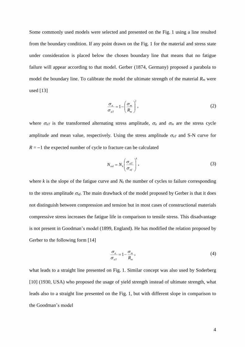
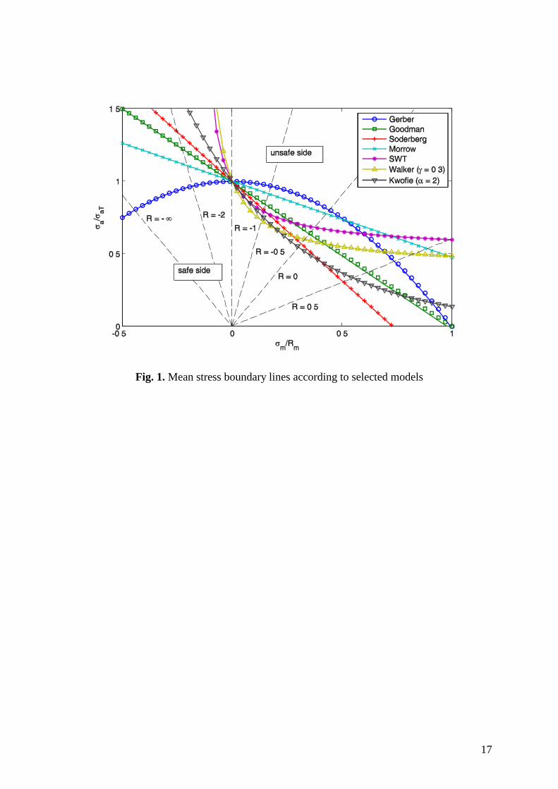
Some commonly used models were selected and presented on the Fig. 1 using a line resulted

from the boundary condition. If any point drawn on the Fig. 1 for the material and stress state

under consideration is placed below the chosen boundary line that means that no fatigue

failure will appear according to that model. Gerber (1874, Germany) proposed a parabola to

model the boundary line. To calibrate the model the ultimate strength of the material Rm were

used [13]

2

1

m

m

aT

a

R

, (2)

where aT is the transformed alternating stress amplitude, a and m are the stress cycle

amplitude and mean value, respectively. Using the stress amplitude aT and S-N curve for

R = 1 the expected number of cycle to fracture can be calculated

k

af

aTkcal NN

, (3)

where k is the slope of the fatigue curve and Nk the number of cycles to failure corresponding

to the stress amplitude af. The main drawback of the model proposed by Gerber is that it does

not distinguish between compression and tension but in most cases of constructional materials

compressive stress increases the fatigue life in comparison to tensile stress. This disadvantage

is not present in Goodman’s model (1899, England). He has modified the relation proposed by

Gerber to the following form [14]

m

m

aT

a

R

1 , (4)

what leads to a straight line presented on Fig. 1. Similar concept was also used by Soderberg

[10] (1930, USA) who proposed the usage of yield strength instead of ultimate strength, what

leads also to a straight line presented on the Fig. 1, but with different slope in comparison to

the Goodman’s model

5

e

m

aT

a

R

1 . (5)

Good known modification of the ‘straight line’ concepts is the model elaborated by Morrow

[15] (1960, USA) where in the place of static material properties the fatigue strength

coefficient is used

f

m

aT

a

'1

. (6)

Another very popular model has been presented by Smith, Watson, and Topper (1970, USA)

in their common paper [16]. This model is usually used in strain based fatigue analysis by

combining the SWT parameter with strain-life equation proposed by Manson [17] multiplied

by Basquin relation [18]

cb

fff

b

f

fb

ff

c

ff

b

f

f

a NNE

NNNE

)2('')2(

')2(')2(')2(

'2

2

max

, (7)

where max = m + a is the maximum stress level and a is the strain amplitude. With the

assumption that the plastic part of the strain amplitude is small and can be neglected while

fatigue life assessment, which is a typical practice in high-cycle fatigue, from the left hand

side of the equation (7) the relationship for transformed stress amplitude can be derived

[15,19]

amaamaaT E )()( . (8)

Equation (8) can be also expressed by stress ratios coefficient R [15]

R

RaaT

1

2

2

1max . (9)

Walker [20] (1979, USA) based on his experimental tests of aluminum alloys has developed a

model for mean stress effects in the following form

aaT

1

max )( , (10)

which can be also expressed by a stress ratios coefficient R

6

1

max1

2

2

1

R

RaaT

. (11)

The main advantage of this model is the material-dependent parameter which allows to

calibrate the model for various groups of materials. By setting the parameter = 0.5 the model

proposed by Walker simplifies to those proposed by Smith-Watson-Topper. Kwofie [21,22]

(2001, Ghana) proposed an exponential function which uses a mean stress sensitivity factor α

for calibration of the model and the factor depends from the kind of material

m

m

aT

a

R

exp . (12)

A careful analysis of presented mean stress effect models leads to the following conclusions:

I. Some of the models, e.g. models proposed by Gerber, Goodman and Soderberg, are using

material constants determined on the basis of monotonic tensile tests. This leads to a simple

implementation of these models, since these properties are commonly available for most

materials. Please note also that those models are developed for the high cycle fatigue or so

called fatigue limit assessment what partially justifies the use of static properties of the

material. However, this is the main reason why it is not possible to describe the fatigue

behavior of the material in a right way, since these parameters do not involve information on

how the material behaves under time-variable loading especially when cyclic hardening or

softening of the material occurs in the middle-cycle fatigue. Only the model by Morrow uses

fatigue strength coefficient but this coefficient is assessed on the basis of experiential data

without mean stress, what shows that also in this case of taking into account the mean stress

will be realized without real information of the materials mean stress sensitivity.

II. Only few propositions use material-dependent parameters which allow calibrating the

model and following the real behavior of the material, e.g. Walker and Kwofie’s models has

an and α factor, respectively. Such kind of coefficients increases the accuracy of fatigue life

7

estimation and makes the models more flexible but the need to determine these factors for

each material makes these models difficult to apply and unpopular.

III. Most of the models allow the calculation of the transformed amplitude according to the

following general formula [4]

),( PK maaT , (13)

where intensifications coefficient K can be expressed as a function of mean stress m and

some material parameters generally representing by P. The exception are the SWT and Walker

models which take into account the mean stress using also the stress amplitude, what leads to

),(),,( PRKPK amaaaT . (14)

IV. All the presented models are not taking directly into account the relationship between the

number of cycles to failure and the mean stress sensitivity of the material. This can be

regarded as a big lack of commonly used models, because the mean stress sensitivity depends

strongly on the cycle range in which the fatigue failure is expected or was observed. To

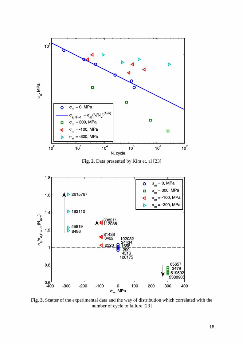
explain the effect on an example experimental results presented by Kim et. al. [23] were used.

Two figures were prepared. Fig. 2 presents experimental fatigue results of smooth samples

under uniaxial stress state for four mean stress values m = 300, 100, 0, and 300 MPa. The

series of experimental results for m = 0 (R = 1) has also been approximated with S-N curve

with following equation of regression a,R=1 = af(N/Nk)(1/k). As a results three material

constants have been obtained: af = 507.6, Nk = 2106, and k = 13.78. Such kind of data

presentation is usual for stress based fatigue tests and can be seen on the basis of it that the

obtained sets of data manifested a small scatter. Fig. 3 has been prepared according to the

graph presented on Fig. 1, but the experimental results and the S-N curve from Fig. 2. has

been used for this purpose. Only for the series of experimental results with the mean stress

value equal to zero, experimental points are grouped around the value 1/K = 1, and their

8

scatter is small. Series of experimental results for significant mean stress values are

characterized with larger scatters. Moreover, for particular series the points are in sequence

corresponding to the number of cycles to failure, which has been properly marked on Fig.3

with arrows. Such huge differences in scatter and the sequence of each series of experimental

points indicate that the K coefficient does not depend only from the mean stress value, but

also from the number of cycles to failure. Gasiak and Pawliczek [24] have presented some

deliberation about this effect and propose to correct them with simple functions estimated

from experimental data without extra theoretical background. Please note that this effect is

often big and cannot be neglected during fatigue life assessment for most of constructional

materials.

It is often found that for the material from which the machine components are made, S-N

curves for repeated (R = 1) and alternating (R = 0) stress are present. For this reason it was

decided to develop a simple model for mean stress correction which is using the stress

amplitudes read directly from such S-N curves for fixed number of cycle. In this case the

general equation for transformed stress amplitude takes the following form

),( fmaaT NK or ),,( ,1, RaNRaNmaaT K . (15)

It is expected that the model will take into account the different sensitivity of the material on

mean stress due to the number of cycles to failure which will result in a better description of

the influence of mean stress on material fatigue.

2. Proposed solution

The key assumption in proposed solution is the use of fatigue strength amplitudes gained for

two boundary states: tension-compression with the stress ratio R = 1 and another one with

9

significant mean stress value, e.g. popular unilateral tension R = 0. Those strengths are read

from the corresponding S-N curves for given number of cycle Ni equal for both curves. It has

been also assumed, that the intermediate state of material effort between the boundary states

can be described by a known continuous function. By selecting the appropriate function

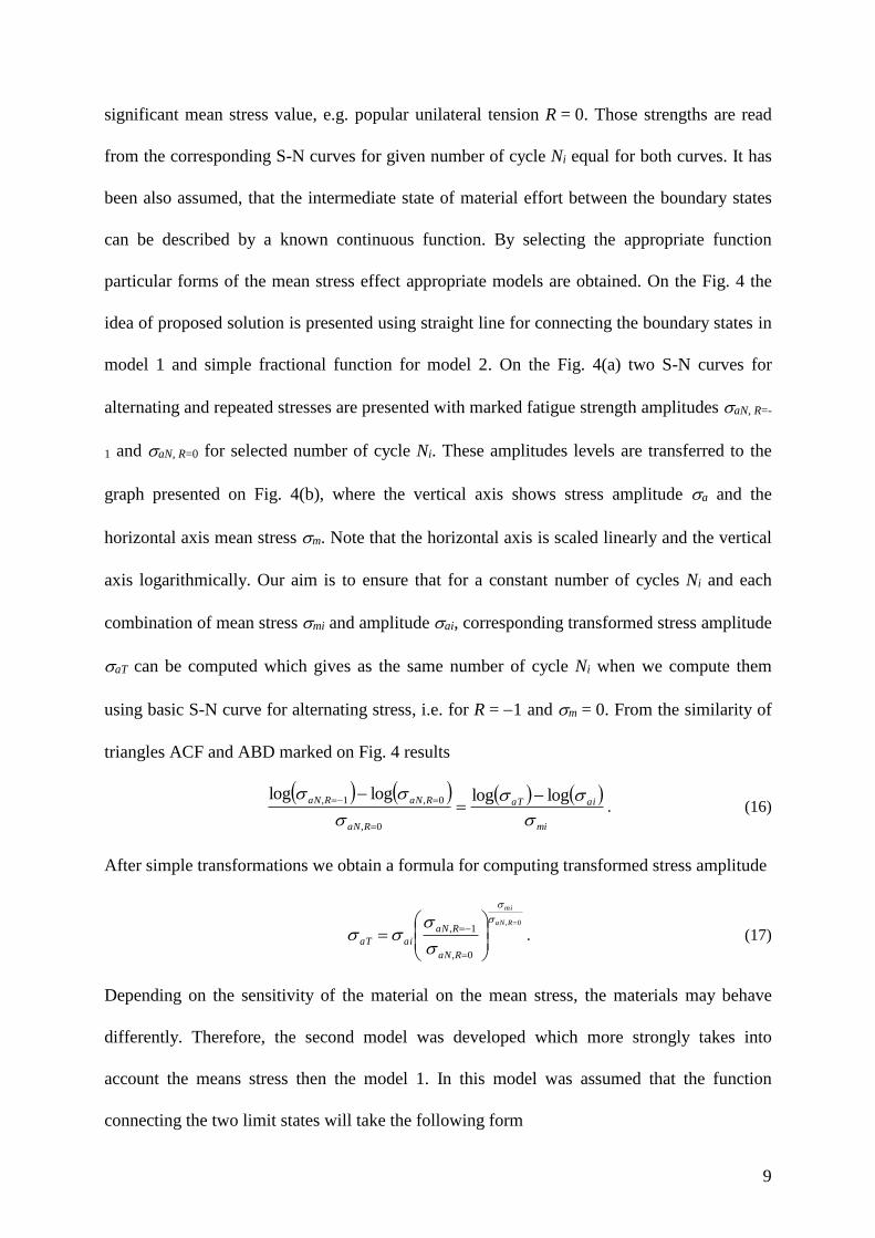
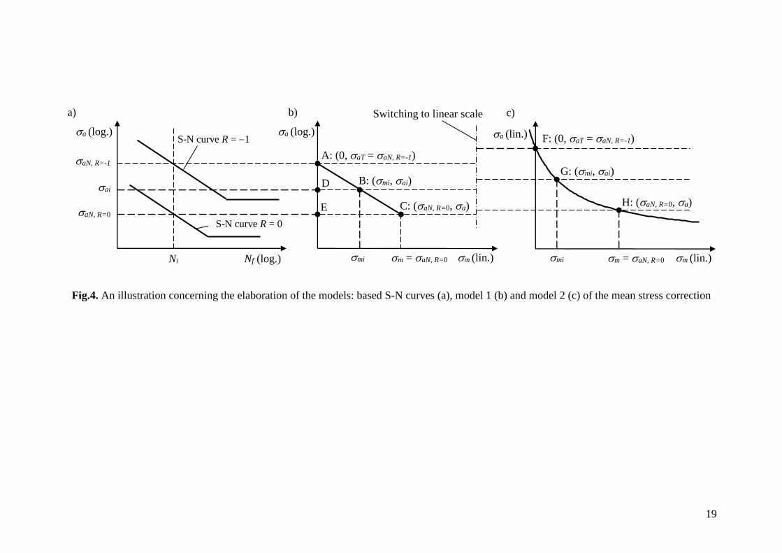
particular forms of the mean stress effect appropriate models are obtained. On the Fig. 4 the

idea of proposed solution is presented using straight line for connecting the boundary states in

model 1 and simple fractional function for model 2. On the Fig. 4(a) two S-N curves for

alternating and repeated stresses are presented with marked fatigue strength amplitudes aN, R=-

1 and aN, R=0 for selected number of cycle Ni. These amplitudes levels are transferred to the

graph presented on Fig. 4(b), where the vertical axis shows stress amplitude a and the

horizontal axis mean stress m. Note that the horizontal axis is scaled linearly and the vertical

axis logarithmically. Our aim is to ensure that for a constant number of cycles Ni and each

combination of mean stress mi and amplitude ai, corresponding transformed stress amplitude

aT can be computed which gives as the same number of cycle Ni when we compute them

using basic S-N curve for alternating stress, i.e. for R = 1 and m = 0. From the similarity of

triangles ACF and ABD marked on Fig. 4 results

mi

aiaT

RaN

RaNRaN

loglogloglog

0,

0,1,

. (16)

After simple transformations we obtain a formula for computing transformed stress amplitude

0,

0,

1,

RaN

mi

RaN

RaN

aiaT

. (17)

Depending on the sensitivity of the material on the mean stress, the materials may behave

differently. Therefore, the second model was developed which more strongly takes into

account the means stress then the model 1. In this model was assumed that the function

connecting the two limit states will take the following form

10

B

A

m

a

(18)

which is much more close to the reality, see the points on Fig. 3. Unknown A and B can be

determined solving following system of equations

B

AB

A

RaN

RaN

RaN

0,

0,

1,

, (19)

where the first equation describes the case when mean stress is equal zero (R = 1, point F on

the Fig. 4c) and the second equation the case of equality of mean stress and stress amplitude

(R = 0, point H on the Fig. 4c). Both equations are true for a selected number of cycles Ni for

which the stress amplitudes were read from the S-N curves. After solving the system of

equations (19) we obtain

1,0,

1,

2

0,

RaNRaN

RaNRaNA

1,0,

2

0,

RaNRaN

RaNB

(20)

On the basis of (18) and (20) we receive

2

0,

0,1,1

RaN

RaNRaN

miaiaT

. (21)

It is easy to notice, that the calibration of formulas (17) and (21) is realized with the use of the

stress amplitudes aN, R=1 and aN, R=0, that is on the basis of two S-N curves for alternating

and repeated stress. In the general case it is also possible to use, instead of the second S-N

curve for R = 0, S-N curve prepared for any value of the stress ratio R 1. By using the

formula for mean stress value defined with the amplitude and irregularity coefficient [11,20]

R

RRaNm

1

1, , (22)

we obtain the appropriate forms of the proposed models, and so on the basis of (17) and (22)

the general form of the first model

11

1

1

,

1,,

R

R

RaN

RaN

aiaT

RaN

mi

, (23)

and on the basis of (21) and (22) the general form of the second model

2

,

,1,

1

11

RaN

RaNRaN

miaiaTR

R

. (24)

where R in equations (23) and (24) takes the value of the irregularity coefficient for which the

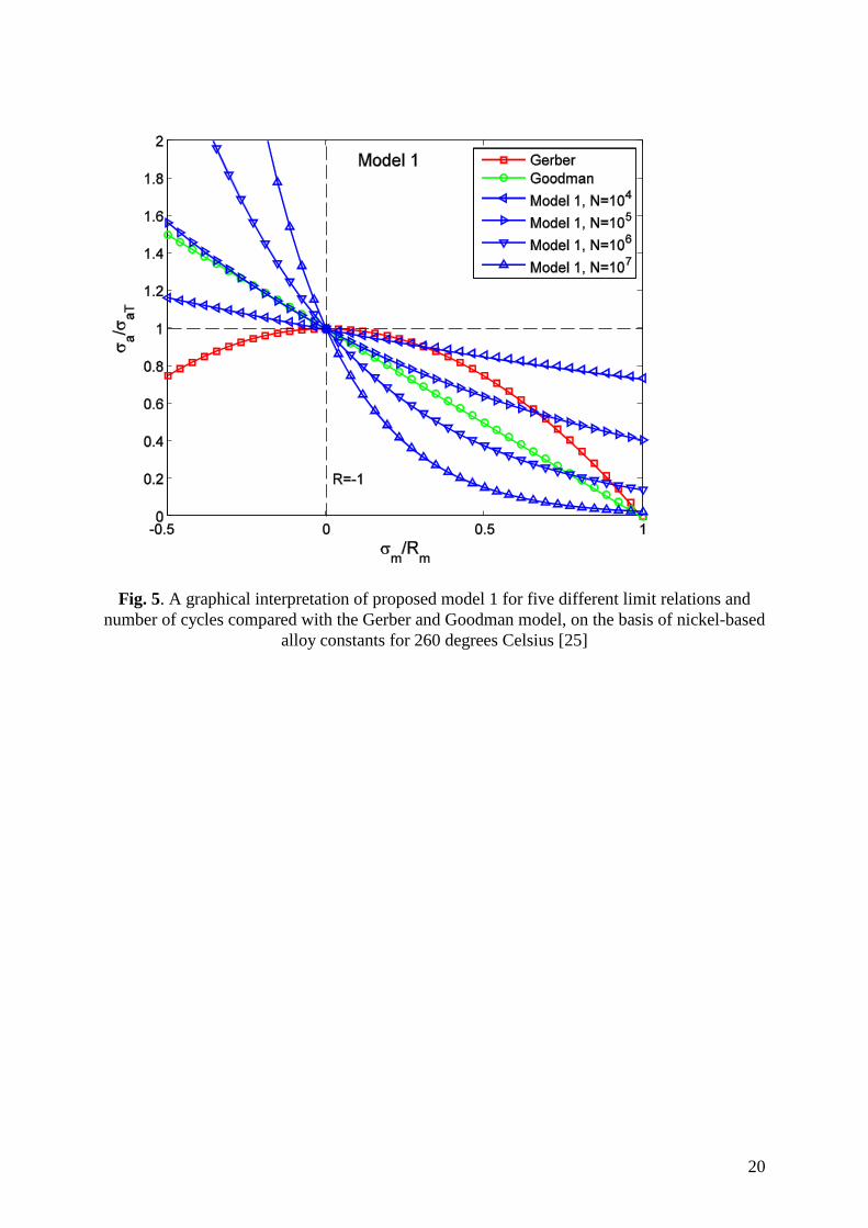
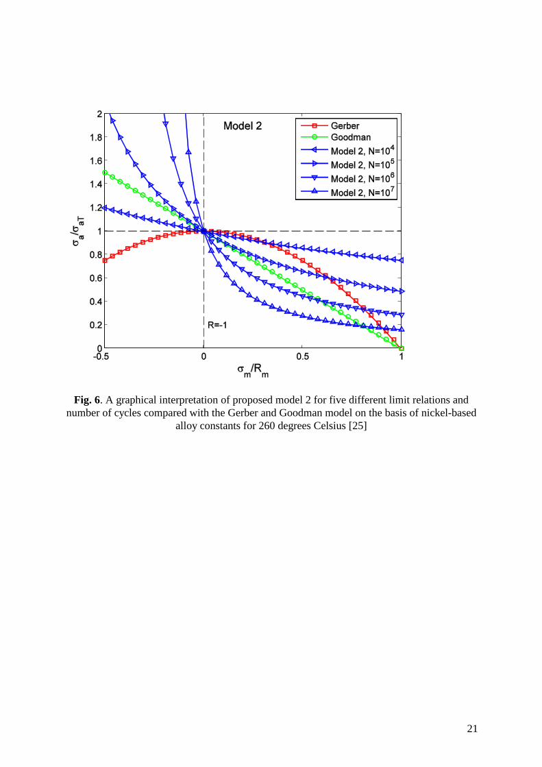
second S-N curve for calibration of the model has been prepared. A graphical interpretation of

the proposed models for five different values of Ni are shown on Figs 5 and 6, together with

the Gerber and Goodman relations for comparisons purposes.

Elaborated models working on fatigue strengths amplitudes aN, R=-1 and aN, R which are easy

to read from appropriate S-N curves and fixed number of cycle Ni. Hence, there is also the

disadvantage of the models – the need to have both fatigue strengths for load ratios R = 1 and

R 1. This quandary can be solved by using known mean stress correction models which are

not using the missing quantity. For example, based on SWT model and special case of

repeated loading (R = 0, σm = σa = aN, R=0), following equation can be written

0,0,0,1, )( RaNRaNRaNRaNaT , (25)

what leads to

2

1,

0,

RaN

RaN

. (26)

In the same way other models can be used for estimating the strength amplitude without the

second S-N curve for R 1, such as for Walker model

1

1,

0,2

RaN

RaN. (27)

12

Such kind of a solution should be used carefully, because all disadvantages of SWT model are

associated with them, what can implicate uncertainty in description of the mean stress

sensitivity and the main advantage of proposed models – the calibration of the models using

strength amplitude from S-N curves – are lost. Therefore, we recommended strongly using the

strength amplitudes from S-N curve and the elaborated Eqs. (23) and (24).

3. Simple verification of the proposed approach

The verification of the proposed method of taking into account the influence of mean stress

has been conducted on the basis of fatigue experimental results available in the literature for

constant amplitude loading conditions in the uniaxial stress state. While choosing the

appropriate data sets particular attention was paid to their completeness, so that they include:

- S-N curve for alternating stress (R = 1),

- S-N curve obtained by constant stress ratio R 1 (usually near R = 0) used for

calibration of the models,

- experimental results for different stress rations,

- ultimate strength of the material obtained under test temperature.

From the available in the literature data sets, the specific fatigue experimental results have

been used to perform the verification:

- Warren and Wei [25] for nickel-based super alloy Waspalloy (AMS 5707) in five

different temperatures,

- Furuya and Abe [26] for experiments with five spring steels after different heat

treatments, and

- Zhang et al. [27] for 2A12-T4 aluminum alloy.

The calculations have been performed for models proposed by Goodman, Gerber, Smith-

Watson-Topper and for two models proposed in this article, Eqs. (23) and (24) respectively.

13

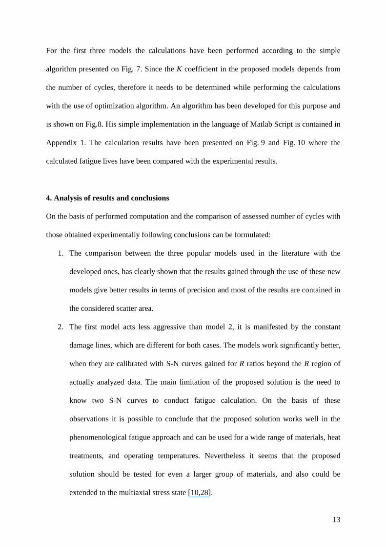
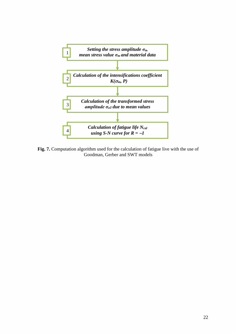
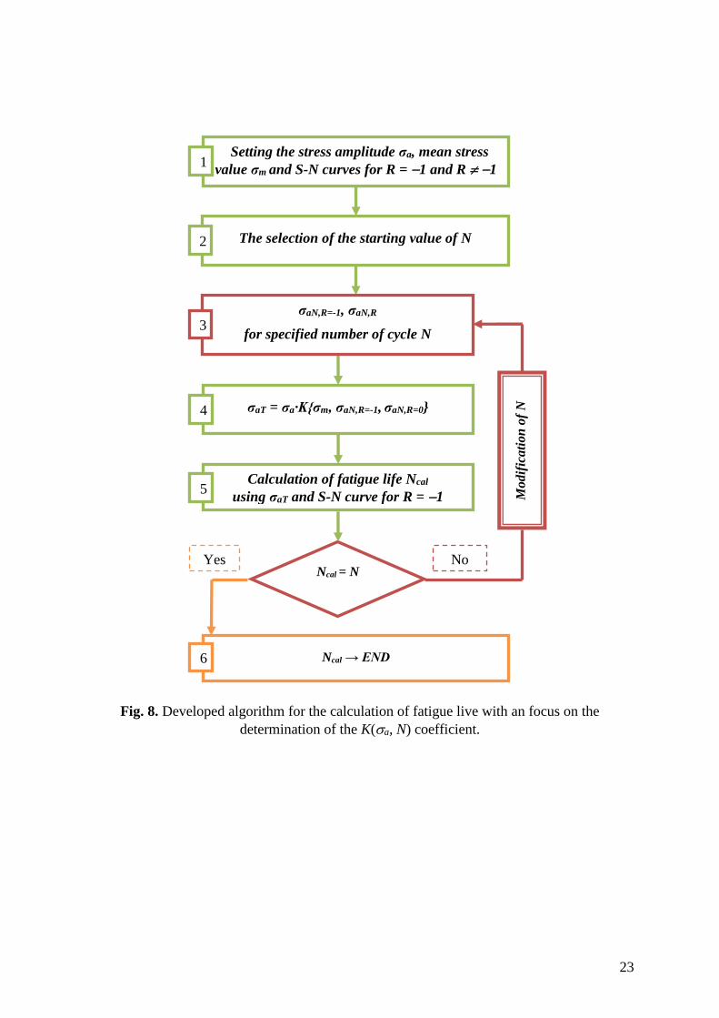
For the first three models the calculations have been performed according to the simple

algorithm presented on Fig. 7. Since the K coefficient in the proposed models depends from

the number of cycles, therefore it needs to be determined while performing the calculations

with the use of optimization algorithm. An algorithm has been developed for this purpose and

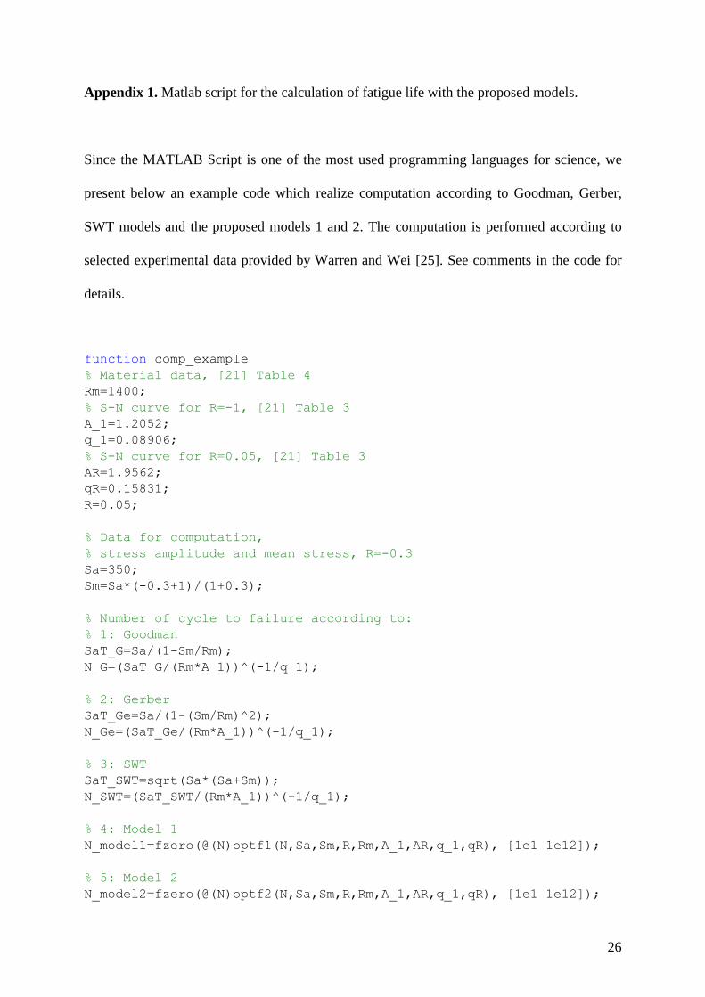
is shown on Fig.8. His simple implementation in the language of Matlab Script is contained in

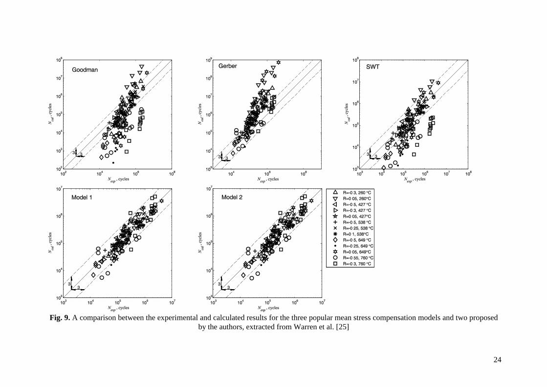
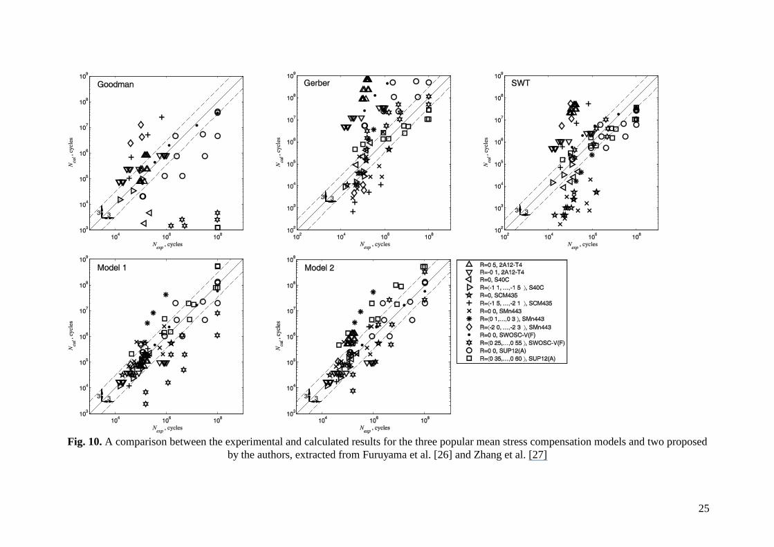
Appendix 1. The calculation results have been presented on Fig. 9 and Fig. 10 where the

calculated fatigue lives have been compared with the experimental results.

4. Analysis of results and conclusions

On the basis of performed computation and the comparison of assessed number of cycles with

those obtained experimentally following conclusions can be formulated:

1. The comparison between the three popular models used in the literature with the

developed ones, has clearly shown that the results gained through the use of these new

models give better results in terms of precision and most of the results are contained in

the considered scatter area.

2. The first model acts less aggressive than model 2, it is manifested by the constant

damage lines, which are different for both cases. The models work significantly better,

when they are calibrated with S-N curves gained for R ratios beyond the R region of

actually analyzed data. The main limitation of the proposed solution is the need to

know two S-N curves to conduct fatigue calculation. On the basis of these

observations it is possible to conclude that the proposed solution works well in the

phenomenological fatigue approach and can be used for a wide range of materials, heat

treatments, and operating temperatures. Nevertheless it seems that the proposed

solution should be tested for even a larger group of materials, and also could be

extended to the multiaxial stress state [10,28].

14

3. The use of an advanced optimization function presented in this article in the terms of

clarification of the goal which is the highest precision of the algorithm, is not a very

popular solution which you can normally find in the area of mean stress influence on

fatigue life.

4. The use of advanced algorithms in the development and calculation of fatigue life is

not longer an unreachable task in terms of precision, especially for an engineer, who

normally operates using stress-life curves with his computer. The script contained in

the appendix is an easy way to improve the precision and quality of calculations

performed by older algorithms, which are still implemented in computer software.

References

[1] H.-J. Christ, C.K. Wamukwamba, H. Mughrabi, The effect of mean stress on the high-

temperature fatigue behaviour of SAE 1045 steel, Materials Science and Engineering: A.

234–236 (1997) 382–385.

[2] J.P. Strizak, L.K. Mansur, The effect of mean stress on the fatigue behavior of 316 LN

stainless steel in air and mercury, Journal of Nuclear Materials. 318 (2003) 151–156.

[3] L. Susmel, Multiaxial Notch Fatigue, 1st ed., CRC Press, 2009.

[4] T. Łagoda, E. Macha, R. Pawliczek, The influence of the mean stress on fatigue life of

10HNAP steel under random loading, International Journal of Fatigue. 23 (2001) 283–

291.

[5] G. Kang, Y. Liu, Uniaxial ratchetting and low-cycle fatigue failure of the steel with

cyclic stabilizing or softening feature, Materials Science and Engineering: A. 472 (2008)

258–268.

[6] J. Polák, J. Man, M. Petrenec, J. Tobiáš, Fatigue behavior of ferritic–pearlitic–bainitic

steel in loading with positive mean stress, International Journal of Fatigue. 39 (2012)

103–108.

[7] N. Miura, Y. Takahashi, High-cycle fatigue behavior of type 316 stainless steel at

288 °C including mean stress effect, International Journal of Fatigue. 28 (2006) 1618–

1625.

[8] P.K. Mallick, Y. Zhou, Effect of mean stress on the stress-controlled fatigue of a short

E-glass fiber reinforced polyamide-6,6, International Journal of Fatigue. 26 (2004) 941–

946.

[9] D. Kujawski, F. Ellyin, A unified approach to mean stress effect on fatigue threshold

conditions, International Journal of Fatigue. 17 (1995) 101–106.

[10] L. Susmel, R. Tovo, P. Lazzarin, The mean stress effect on the high-cycle fatigue

strength from a multiaxial fatigue point of view, International Journal of Fatigue. 27

(2005) 928–943.

15

[11] N.E. Dowling, C.A. Calhoun, A. Arcari, Mean stress effects in stress-life fatigue and

the Walker equation, Fatigue & Fracture of Engineering Materials & Structures. 32

(2009) 163–179.

[12] D. McClaflin, A. Fatemi, Torsional deformation and fatigue of hardened steel including

mean stress and stress gradient effects, International Journal of Fatigue. 26 (2004) 773–

784.

[13] W.Z. Gerber, Bestimmung der zulässigen spannungen in eisen-constructionen

(Calculation of the allowable stresses in iron structures), Z Bayer Archit. Ing-Ver. 6

(1874) 101–110.

[14] J. Goodman, Mechanics applied to engineering, Longmans, Green & Co., 1899.

[15] N.E. Dowling, Mean stress effects in strain–life fatigue, Fatigue & Fracture of

Engineering Materials & Structures. 32 (2009) 1004–1019.

[16] K.N. Smith, P. Watson, T.H. Topper, A stress-strain function for the fatigue of metals,

Journal Materials. 5 (1970) 767–776.

[17] S.S. Manson, Fatigue: A complex subject—Some simple approximations, Experimental

Mechanics. 5 (1965) 193–226.

[18] O.H. Basquin, The Exponential Law of Endurance Tests, Am. Soc. Test. Mater. Proc.

10 (1910) 625–630.

[19] A. Ince, G. Glinka, A modification of Morrow and Smith–Watson–Topper mean stress

correction models, Fatigue & Fracture of Engineering Materials & Structures. 34 (2011)

854–867.

[20] K. Walker, The Effect of Stress Ratio During Crack Propagation and Fatigue for 2024-

T3 and 7075-T6 Aluminum, in: M. Rosenfeld (Ed.), Effects of Environment and

Complex Load History on Fatigue Life, ASTM International, 100 Barr Harbor Drive, PO

Box C700, West Conshohocken, PA 19428-2959, 1970: pp. 1–1–14.

[21] S. Kwofie, An exponential stress function for predicting fatigue strength and life due to

mean stresses, International Journal of Fatigue. 23 (2001) 829–836.

[22] S. Kwofie, Equivalent stress approach to predicting the effect of stress ratio on fatigue

threshold stress intensity range, International Journal of Fatigue. 26 (2004) 299–303.

[23] K.S. Kim, K.M. Nam, G.J. Kwak, S.M. Hwang, A fatigue life model for 5% chrome

work roll steel under multiaxial loading, International Journal of Fatigue. 26 (2004) 683–

689.

[24] G. Gasiak, R. Pawliczek, Application of an energy model for fatigue life prediction of

construction steels under bending, torsion and synchronous bending and torsion,

International Journal of Fatigue. 25 (2003) 1339–1346.

[25] J. Warren, D.Y. Wei, A microscopic stored energy approach to generalize fatigue life

stress ratios, International Journal of Fatigue. 32 (2010) 1853–1861.

[26] Y. Furuya, T. Abe, Effect of mean stress on fatigue properties of 1800 MPa-class spring

steels, Materials & Design. 32 (2011) 1101–1107.

[27] J. Zhang, X. Shi, R. Bao, B. Fei, Tension–torsion high-cycle fatigue failure analysis of

2A12-T4 aluminum alloy with different stress ratios, International Journal of Fatigue. 33

(2011) 1066–1074.

[28] A. Fatemi, P. Kurath, Multiaxial Fatigue Life Predictions Under the Influence of Mean-

Stresses, J. Eng. Mater. Technol. 110 (1988) 380–388.

16

Figure captions:

Fig. 1. Mean stress boundary lines according to presented models

Fig. 2. Data presented by Kim et. al [23]

Fig. 3. Scatter of the experimental data and the way of distribution which correlated with the

number of cycle to failure [23]

Fig.4. An illustration concerning the elaboration of the models: based S-N curves (a), model

1 (b) and model 2 (c) of the mean stress

Fig. 5. A graphical interpretation of proposed model 1 for five different limit relations and

number of cycles compared with the Gerber and Goodman model, on the basis of

nickel-based alloy constants for 260 degrees Celsius [25]

Fig. 6. A graphical interpretation of proposed model 2 for five different limit relations and

number of cycles compared with the Gerber and Goodman model on the basis of

nickel-based alloy constants for 260 degrees Celsius [25]

Fig. 7. Computation algorithm used for the calculation of fatigue live with the use of

Goodman, Gerber and SWT models.

Fig. 8. Developed algorithm for the calculation of fatigue live with an focus on the

determination of the K(a, N) coefficient.

Fig. 9. A comparison between the experimental and calculated results for the three popular

mean stress compensation models and two proposed by the authors, extracted from

Warren et al. [25]

Fig. 10. A comparison between the experimental and calculated results for the three popular

mean stress compensation models and two proposed by the authors, extracted from

Furuyama et al. [26] and Zhang et al. [27]

17

Fig. 1. Mean stress boundary lines according to selected models

18

Fig. 2. Data presented by Kim et. al [23]

Fig. 3. Scatter of the experimental data and the way of distribution which correlated with the

number of cycle to failure [23]

19

Fig.4. An illustration concerning the elaboration of the models: based S-N curves (a), model 1 (b) and model 2 (c) of the mean stress correction

S-N curve R = 1

S-N curve R = 0

Nf (log.)

a (log.)

m (lin.)

a (log.)

aN, R=-1

aN, R=0

ai

A: (0, aT = aN, R=-1)

B: (mi, ai)

C: (aN, R=0, a)

m = aN, R=0

D

E

Ni mi

a) b)

a (lin.)

m (lin.)

F: (0, aT = aN, R=-1)

G: (mi, ai)

H: (aN, R=0, a)

m = aN, R=0 mi

c) Switching to linear scale

20

Fig. 5. A graphical interpretation of proposed model 1 for five different limit relations and

number of cycles compared with the Gerber and Goodman model, on the basis of nickel-based

alloy constants for 260 degrees Celsius [25]

21

Fig. 6. A graphical interpretation of proposed model 2 for five different limit relations and

number of cycles compared with the Gerber and Goodman model on the basis of nickel-based

alloy constants for 260 degrees Celsius [25]

22

Fig. 7. Computation algorithm used for the calculation of fatigue live with the use of

Goodman, Gerber and SWT models

Setting the stress amplitude σa,

mean stress value σm and material data

1

Calculation of the intensifications coefficient

K(m, P) 2

Calculation of the transformed stress

amplitude σaT due to mean values

3

Calculation of fatigue life Ncal

using S-N curve for R = 1 4

23

Fig. 8. Developed algorithm for the calculation of fatigue live with an focus on the

determination of the K(a, N) coefficient.

Setting the stress amplitude σa, mean stress

value σm and S-N curves for R = 1 and R 1

Calculation of fatigue life Ncal

using σaT and S-N curve for R = 1

Ncal = N No

Modif

icati

on

of

N

Yes

Ncal → END

1

5

6

The selection of the starting value of N 2

σaN,R=-1, σaN,R

for specified number of cycle N 3

σaT = σa·K{σm, σaN,R=-1, σaN,R=0} 4

24

Fig. 9. A comparison between the experimental and calculated results for the three popular mean stress compensation models and two proposed

by the authors, extracted from Warren et al. [25]

25

Fig. 10. A comparison between the experimental and calculated results for the three popular mean stress compensation models and two proposed

by the authors, extracted from Furuyama et al. [26] and Zhang et al. [27]

26

Appendix 1. Matlab script for the calculation of fatigue life with the proposed models.

Since the MATLAB Script is one of the most used programming languages for science, we

present below an example code which realize computation according to Goodman, Gerber,

SWT models and the proposed models 1 and 2. The computation is performed according to

selected experimental data provided by Warren and Wei [25]. See comments in the code for

details.

function comp_example

% Material data, [21] Table 4

Rm=1400;

% S-N curve for R=-1, [21] Table 3

A_1=1.2052;

q_1=0.08906;

% S-N curve for R=0.05, [21] Table 3

AR=1.9562;

qR=0.15831;

R=0.05;

% Data for computation,

% stress amplitude and mean stress, R=-0.3

Sa=350;

Sm=Sa*(-0.3+1)/(1+0.3);

% Number of cycle to failure according to:

% 1: Goodman

SaT_G=Sa/(1-Sm/Rm);

N_G=(SaT_G/(Rm*A_1))^(-1/q_1);

% 2: Gerber

SaT_Ge=Sa/(1-(Sm/Rm)^2);

N_Ge=(SaT_Ge/(Rm*A_1))^(-1/q_1);

% 3: SWT

SaT_SWT=sqrt(Sa*(Sa+Sm));

N_SWT=(SaT_SWT/(Rm*A_1))^(-1/q_1);

% 4: Model 1

N_model1=fzero(@(N)optf1(N,Sa,Sm,R,Rm,A_1,AR,q_1,qR), [1e1 1e12]);

% 5: Model 2

N_model2=fzero(@(N)optf2(N,Sa,Sm,R,Rm,A_1,AR,q_1,qR), [1e1 1e12]);

27

% 6: S-N curve from experimental results [1]

N_exp=(Sa/(Rm*1.6185))^(-1/0.12903);

% Print the results

clc

disp('Number of cycle to failure according experimental S-N curve:')

disp(['Exp. : ' num2str(round(N_exp))])

disp('Number of cycle to failure according:')

disp(['Goodman: ' num2str(round(N_G))])

disp(['Gerber : ' num2str(round(N_Ge))])

disp(['SWT : ' num2str(round(N_SWT))])

disp(['Model 1: ' num2str(round(N_model1))])

disp(['Model 2: ' num2str(round(N_model2))])

%%% Internal functions used by fzero

function OptPar=optf1(N, Sa, Sm, R, Rm, A_1, AR, q_1, qR)

% N - calculated cycle number

% Sa, Sm - amplitude and mean value

% R - stress ratio for the S-N curve used by calibration

% Rm - ultimate strength

% A_1, q_1 - regression coefficients of the R=-1 S-N curve

% AR, qR - regression coefficients of the S-N curve used by

% calibration of the model

sigaf_1=Rm*A_1*N^(-q_1);

sigaf_R=Rm*AR*N^(-qR);

K=(sigaf_1/sigaf_R)^(Sm/sigaf_R*(1-R)/(R+1));

SaT=K*Sa;

OptPar=log(N)-log((SaT/(Rm*A_1))^(1/-q_1));

function OptPar=optf2(N, Sa, Sm, R, Rm, A_1, AR, q_1, qR)

% Sescription the same like in optf1 function

sigaf_1=Rm*A_1*N^(-q_1);

sigaf_R=Rm*AR*N^(-qR);

K=1+Sm*((1-R)/(R+1))*(sigaf_1-sigaf_R)/(sigaf_R^2);

SaT=K*Sa;

OptPar=log(N)-log((SaT/(Rm*A_1))^(1/-q_1));

% End of the comp_example function