Mean field bipartite spin models treated with mechanical techniques

Mean field bipartite spin models treated with mechanical techniques

Adriano Barra∗, Andrea Galluzzi †, Francesco Guerra‡, Andrea Pizzoferrato§, Daniele Tantari ¶

December 16, 2013

Abstract

Inspired by a continuously increasing interest in modeling and framing complex systems in a thermody-namic rationale, in this paper we continue our investigation in adapting well known techniques (originallystemmed in fields of physics and mathematics far from the present) for solving for the free energy of meanfield spin models in a statistical mechanics scenario.

Focusing on the test cases of bipartite spin systems embedded with all the possible interactions (self andreciprocal), we show that both the fully interacting bipartite ferromagnet as well as the spin glass counterpart,at least at the replica symmetric level, can be solved via the fundamental theorem of calculus, trough ananalogy with the Hamilton-Jacobi theory and lastly with a mapping to a Fourier diffusion problem. Allthese technologies are shown symmetrically for ferromagnets and spin-glasses in full details and contributeas powerful tools in the investigation of complex systems.

1 IntroductionIn the last years, equilibrium statistical mechanics has been successfully extended beyond the conventional areaof the physics of matter, for instance in quantitative sociology (see e.g. [13, 25, 20, 21]) or theoretical biology(see e.g. [38, 3, 37, 4]). However, these (as well as many others, see e.g. [16, 23]) new research fields continuouslyrequire more refined mathematical methods and models in order to give an always more relevant quantitativedescription and understanding of the phenomena they aim to tackle.Among the several novelty these fields of research required, there has been a microscopic description of dynamicalsystems where two species compete or collaborate, for instance a’ la Lotka-Volterra: restricting to equilibriumproperties, this need led to a renewal formulation of bipartite spin systems [22], beyond their original introductionwithin the more standard world of physics of matter [32], which allows to study the emergent collective propertiesof two interactive large groups of variables. For instance, in quantitative sociology the latter may captureessential features of migrant’s integration inside a host community [14] or the dialogue between two differentensembles of closely interacting cells, as for instance B and T cells within the immune system [1].In this paper we do not deal with comparing modeling to real data, instead we continue our investigationconsisting in obtaining new statistical mechanics techniques all based on adapting existing technologies originallydeveloped to work in field far away from the actual focus, such to make them able to solve for the free energyof suitably defined mean field spin Hamiltonians. We will mainly focus on sum rules originated from a mappingof the statistical mechanics problem with the fundamental theorem of calculus as firstly shown in [30] and thenextended in [9], with the Hamilton-Jacobi framework, firstly developed in [28] and then extended in [9][12], andwith the Fourier conduction investigated in [26][7], which is a side effect of the mechanical analogy previouslyintroduced.Dealing with the subjects and not only with the methodologies, the present work constitutes an extension mainlyof [6], where bipartite mean field model have been carefully inspected from a (standard) statistical mechanics∗Sapienza Università di Roma, Dipartimento di Fisica and GNFM Gruppo di Roma, Italy†Sapienza Università di Roma, Dipartimento di Matematica and GNFM Gruppo di Roma, Italy‡Sapienza Università di Roma, Dipartimento di Fisica and INFN Sezione di Roma, Italy§The University of Warwick, Mathematics Institute, Coventry, United Kingdom¶Sapienza Università di Roma, Dipartimento di Matematica and GNFM Gruppo di Roma, Italy

1

arX

iv:1

310.

5901

v1 [

cond

-mat

.dis

-nn]

22

Oct

201

3

perspective and [7] where the techniques we are going to use have been tested on single-party models: the tworoutes of investigation are here merged together in a unified and stronger theory.The paper is divided into two symmetric parts: In the first one, a bipartite ferromagnetic model, which notonly considers the interaction among spins of different parties but also between the ones of the same group, isstudied through three different interpolation approaches, respectively the fundamental theorem of calculus, theHamilton-Jacobi scheme and the Fourier transform. In the second one, the same procedures are applied to thedisordered (glassy) counterpart of the first model. Unfortunately, as a Parisi-like theory [36] for these models isstill under construction, and also because it is usually sacrificed in many practical applications involving modelsbeyond the Sherrington-Kirkpatrick paradigm, the thermodynamics of these systems is studied at the replicasymmetric level.

2 Ferromagnetic case

2.1 The ModelThe spin system we study is an extension of the one analyzed in [6]. There, two dichotomic parties of variables,σii=1,...,Nσ and τii=1,...,Nτ , which were coupled through a ferromagnetic interaction, were considered: herewe take into account also the ferromagnetic interaction between spins of the same group. All this results in aHamiltonian made up of the following contributions

HN (σ, τ ,β) = − 1

Nβστ

Nσ∑i=1

Nτ∑j=1

σiτj −1

2Nβσ

Nσ∑i,j

σiσj −1

2Nβτ

Nτ∑i,j

τiτj , (1)

where σi, τi ∈ −1; 1 are the two families of dichotomic spin variables; βσ, βτ and βστ are the strength of theinteractions weighting the intensity of the three different contributions to the Hamiltonian; Nσ and Nτ are thenumber of spins for each party with N = Nσ + Nτ . Note that equation (1) defines a mean-field model, whereeach couple of spins interact in a ferromagnetic way (all the couplings are positive), and the normalization 1/Nensure the linear extensivity of the thermodynamical observables (e.g. energy, entropy, etc.) with respect tothe size of the system. Introducing α = Nσ/N and thus (1− α) = Nτ/N and denoting with O(σ, τ ) a genericobservable of the system, the definitions of the statistical mechanic and thermodynamic quantities are givenstraightforwardly:

Partition function ZN (β, α) :=∑σ,τ e

−βHN (σ,τ,β,α),

Boltzmann average 〈O (σ, τ )〉 := Z−1N (β, α)

∑σ,τ O (σ, τ ) e−βHN (σ,τ,β,α),

Magnetization of the σ party mσ(σ) := 1Nσ

∑Nσi=1 σi,

Magnetization of the τ party mτ (τ ) := 1Nτ

∑Nτi=1 τi,

Pressure (free energy) A(β, α) = limN→∞AN (β, α) := 1N lnZN (β, α) = −βfN (β),

where fN (β) is the free energy.In the following, for the sake of simplicity and without loss of generality, we will put β = 1: we can restore thedependence by β simply rescaling the couplings βx → ββx, with x = σ, τ, στ . In the present paper we wantto describe three different techniques that can be used to solve the model and in particular to compute thethermodynamic limit of the intensive pressure as to characterize the thermodynamic states, i.e. the averages(and in general the moments) of the order parameters. Each one of the three routes approaches the problemfrom a different perspective but all of these can be thought as proofs of the following

2

Theorem 1. The thermodynamic limit of the intensive pressure of the full interacting ferromagnetic bipartitemodel defined in (1) reads as

A(β, α) = ln 2 + α ln cosh (βσαmσ + βστ (1− α) mτ ) + (1− α) ln cosh (βσταmσ + βτ (1− α) mτ ) + (2)

−[βστα (1− α) mσmτ +

1

2βσα

2m2σ +

1

2βτ (1− α)

2m2τ

],

where the two quantities mσ and mτ are the solution of the following system of self-consistent equationsmσ = tanh (βσαmσ + βστ (1− α) mτ ) ,

mτ = tanh (βσταmσ + βτ (1− α) mτ ) .(3)

Remark 1. Equations (3) can be obtained by extremizing the free energy expressed in Theorem 1 with respect tothe trial parameters mσ and mτ . We stress that where βσβτ ≥ β2

στ the optimal parameters impose a maximumfor the pressure landscape while in the opposite region it is a saddle point only. On the critical surface βσβτ = β2

στ

the pressure has a flat direction and the model can be described through a single order parameter that is a linearcombination of the two magnetizations, i.e. ε =

√βσαmσ +

√βτ (1− α) mτ and

A(β, α) = ln 2 + α ln cosh(√βσ ε) + (1− α) ln cosh(

√βτ ε)−

ε2

2(4)

with ε satisfyingε =

√βσα tanh(

√βσ ε) +

√βτ (1− α) tanh(

√βτ ε). (5)

It is worth noticing that in the limit of βστ = 0 the two parties are non interacting and a convex linearcombination of two standard Curie-Weiss pressure at suitable temperatures is obtained, while, for βσ = βτ = 0,the results developed in [6] for a bipartite system without monopartite interactions are recovered.

2.2 First approach: Sum ruleThe method that in this section we adapt to fully interacting bipartite ferromagnets has been successfullyapplied in [27, 10] for a huge class of single disordered system or systems in reciprocal interactions but withoutself-contributions. Here we show how it works in the larger case of complete topological interactions, startingwith simpler case of the ferromagnetic couplings highlighting the perspective we want to follow. In the secondhalf of the manuscript we will apply it to the disordered counterpart, which will require some more mathematicalefforts. In a quick introductional summary, the technique consists of three steps:

• Through the introduction of an interpolating parameter t ∈ [0, 1], a new trial Hamiltonian is defined asthe sum of two pieces, to which it reduces in the limit t→ 1 and t→ 0: the former is the original model,which has to be solved, and the latter is spin system with a simpler one-body interaction with an externaleffective field that mirrors the real microscopic interactions in a pure mean field fashion, hence

H(t) = (t)Horiginal + (1− t)Hone-body.

From the interpolating Hamiltonian, the definitions of interpolating partition function ZN (t) and pressureAN (t) naturally follow simply shifting exp(−βH)→ exp(−βH(t)).

• Once the interpolating structure is defined, an interpolating procedure is needed: this role is played bythe Fundamental Theorem of Calculus. The key point is that the pressure of the original model can bewritten as

AN = AN (1) = AN (0) +

∫ 1

0

∂AN∂t

dt.

In this way the problem is split into the calculation of two terms: AN (0) and∫ 1

0∂AN (t)∂t dt

3

𝑡=1𝑡

𝜎

𝜏

𝑡=0

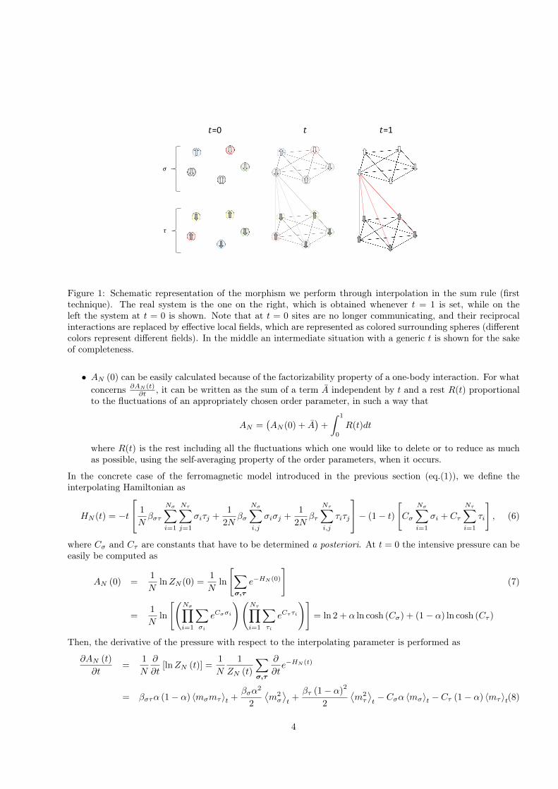
Figure 1: Schematic representation of the morphism we perform through interpolation in the sum rule (firsttechnique). The real system is the one on the right, which is obtained whenever t = 1 is set, while on theleft the system at t = 0 is shown. Note that at t = 0 sites are no longer communicating, and their reciprocalinteractions are replaced by effective local fields, which are represented as colored surrounding spheres (differentcolors represent different fields). In the middle an intermediate situation with a generic t is shown for the sakeof completeness.

• AN (0) can be easily calculated because of the factorizability property of a one-body interaction. For whatconcerns ∂AN (t)

∂t , it can be written as the sum of a term A independent by t and a rest R(t) proportionalto the fluctuations of an appropriately chosen order parameter, in such a way that

AN =(AN (0) + A

)+

∫ 1

0

R(t)dt

where R(t) is the rest including all the fluctuations which one would like to delete or to reduce as muchas possible, using the self-averaging property of the order parameters, when it occurs.

In the concrete case of the ferromagnetic model introduced in the previous section (eq.(1)), we define theinterpolating Hamiltonian as

HN (t) = −t

1

Nβστ

Nσ∑i=1

Nτ∑j=1

σiτj +1

2Nβσ

Nσ∑i,j

σiσj +1

2Nβτ

Nτ∑i,j

τiτj

− (1− t)

[Cσ

Nσ∑i=1

σi + Cτ

Nτ∑i=1

τi

], (6)

where Cσ and Cτ are constants that have to be determined a posteriori. At t = 0 the intensive pressure can beeasily be computed as

AN (0) =1

NlnZN (0) =

1

Nln

[∑σ,τ

e−HN (0)

](7)

=1

Nln

[(Nσ∏i=1

∑σi

eCσσi

)(Nτ∏i=1

∑τi

eCττi

)]= ln 2 + α ln cosh (Cσ) + (1− α) ln cosh (Cτ )

Then, the derivative of the pressure with respect to the interpolating parameter is performed as

∂AN (t)

∂t=

1

N

∂

∂t[lnZN (t)] =

1

N

1

ZN (t)

∑σ,τ

∂

∂te−HN (t)

= βστα (1− α) 〈mσmτ 〉t +βσα

2

2

⟨m2σ

⟩t

+βτ (1− α)

2

2

⟨m2τ

⟩t− Cσα 〈mσ〉t − Cτ (1− α) 〈mτ 〉t(8)

4

Now the last expression has to be written in terms of the fluctuations of the order parameters. Defining a, band c as free coefficients, the generic form of the fluctuations of the order parameters is

a 〈(mσ − mσ) (mτ − mτ )〉t + b⟨

(mσ − mσ)2⟩t

+ c⟨

(mτ − mτ )2⟩t

= (9)

= a 〈mσmτ 〉t + b⟨m2σ

⟩t

+ c⟨m2τ

⟩t

+ (−amτ − 2bmσ) 〈mσ〉t + (−amσ − 2cmτ ) 〈mτ 〉t +[amσmτ + bm2

σ + cm2τ

].

Hence, we can identify each coefficient of the equation (9) with the ones of the specific expression (8), in sucha way that we can fix the coefficients Cσ and Cτ as

Cσ = αβσmσ + βστ (1− α) mτ ; Cτ = βσταmσ + (1− α)βτmτ .

Using equations (7) and (8) we can then write down the following sum rule

AN (β, α) = ln 2 + α ln cosh (βσαmσ + βστ (1− α) mτ ) + (1− α) ln cosh (βσταmσ + βτ (1− α) mτ ) (10)

−[βστα (1− α) mσmτ +

1

2βσα

2m2σ +

1

2βτ (1− α)

2m2τ

]+RN (t)

where

RN (t) =

∫ 1

0

dt[a 〈(mσ − mσ) (mτ − mτ )〉t + b

⟨(mσ − mσ)

2⟩t

+ c⟨

(mτ − mτ )2⟩t

]. (11)

Since in the ferromagnetic models the magnetizations are self-averaging in the thermodynamic limit, we canargue that, for a particular choice of the parameters mσ and mτ (that is by extremizing the pressure withrespect to them) we can neglect the rest in (10), namely

limN→∞

RN (t) = 0,

and in the same limit AN → A (where A represents the pressure evaluated for N → ∞), that completes theproof of Theorem 1. Note that, by deriving equation (10) with respect to mσ and mτ we get

∂A∂mσ

= βσα2 (〈σi〉t=0 − mσ) + βστα (1− α) (〈τi〉t=0 − mτ ) = 0,

∂A∂mτ

= βστα (1− α) (〈σi〉t=0 − mσ) + βτ (1− α)2

(〈τi〉t=0 − mτ ) = 0,

from which we can argue that, as soon as βσβτ 6= β2στ , the optimal order parameters satisfy

mσ = 〈σi〉t=0

mτ = 〈τi〉t=0 , (12)

i.e. the magnetizations of the interpolating system at t = 0 are the same of the original system’s ones. Fromthe equations (12) we can see that, on the critical surface βσβτ = β2

στ , we have just one single degenerateself consistent equation, that is eq.(5) for an order parameter ε(σ, τ ) =

√βσαmσ(σ, τ ) +

√βτ (1− α)mτ (σ, τ )

which is a linear combination of the two magnetizations. In this region of the phase space ε(σ, τ ) is self averagingbut the two magnetizations can fluctuate. This phenomenon is very clear for example in the special case inwhich βσ = βτ = βστ = β, where we cannot distinguish any longer between the two parties: the system is asingle Curie Wiess model, of size N , characterized by a single order parameter that is the global magnetizationM(σ, τ ) = αmσ(σ) + (1− α)mτ (τ ) = β−1/2ε(σ, τ ).

2.3 Second approach: The Hamilton-Jacobi frameworkBesides the fundamental theorem of calculus, another interpolation method, developed in [28], can be used.The latter is based on a mechanistic interpretation of the statistical mechanic and thermodynamic quantitiesdefined at the beginning of this section.The main idea is the following: the problem of obtaining an explicit expression for the pressure of the model

5

(1) in the thermodynamic limit and in terms of its order and tunable parameters, is translated in solving anHamilton-Jacobi equation, where the pressure plays as the action, with suitable boundary conditions. For thispurpose, with the freedom of thinking at the interpolating parameters t ∈ R+ and x ∈ R as fictitious time andspace respectively, we first define an interpolating Hamiltonian as

HN (t, x) = − t

[Nταβστmσmτ +

Nσ2αβσm

2σ +

Nτ2

(1− α)βτm2τ

](13)

− (1− t)[Nσ2β′σm

2σ +

Nτ2β′τm

2τ

]− xNDN (σ, τ), (14)

where, introducing a free parameter a ∈ (0,∞) (whose practical convenience will be evident later), we defined

β′σ = α[a2βστ + βσ

]; β′τ = (1− α)

[a−2βστ + βτ

],

and the order parameter D(σ, τ) (that is just a linear combination of the magnetizations)

D(σ, τ) =√βστ

[αamσ − (1− α) a−1mτ

]. (15)

Then, from the definition of the interpolating Hamiltonian we introduce, as usual, an interpolating pressureSN (t, x) = N−1 ln

∑σ τ e

−HN (t,x), which we named S as it plays the role of an action in the (t, x) space.Performing the temporal and spatial derivatives of SN (t, x) and denoting with a subscript (t, x) the averagesperformed within the extended Boltzmann measure weighted by HN (t, x)1, we get

∂SN (t, x)

∂t=− 1

2

⟨D2⟩

(t,x)

∂SN (t, x)

∂x= 〈D〉(t,x)

∂2SN (t, x)

∂x2=N

(⟨D2⟩

(t,x)− 〈D〉2(t,x)

),

thus, directly by construction, we can write the following Hamilton-Jacobi equation for SN (t, x):

∂tSN (t, x) +1

2(∂xSN (t, x))2 + VN (t, x) = 0, (16)

where the potential VN (t, x) is defined as

VN (t, x) = −1

2

(⟨D2⟩

(t,x)− 〈D〉2(t,x)

)=

1

2N

∂2SN (t, x)

∂x2. (17)

Because of the self-averaging of the order parameters2, the potential becomes negligible when the size of thesystem grows to infinity, hence S(t, x) satisfies, in the thermodynamic limit, a free Hamilton-Jacobi equation.We can easily solve it by noting that the velocity field D(t, x) = ∂xS(t, x) = 〈D〉(t,x) is constant along thetrajectories x = x0 +D(t, x)t, such that D(t, x) can be determined from the relation

D(t, x) = D(0, x0) = ∂xS(0, x)|x = x0(t, x) (18)

that plays as a self consistent equation for D.The general expression for the action S(t, x) can be obtained as its value evaluated in a point S(0, x0) (theCauchy condition) plus the integral of the Lagrangian L(t, x) over time. Note that here, as the trajectories ofsuch a fictitious motion are straight lines, or alternatively because the potential is zero, the Lagrangian readsoff simply as L(t, x) = 〈D〉2t,x/2, hence overall we can write

S (t, x) = S (t = 0, x = x0) +

∫ t

0

L (t′, x) dt′ = S (0, x0) +t

2〈D2〉(t,x). (19)

1Note that this extended average reduces to the canonical one whenever measured at t = 1 and x = 0.2Alternatively, instead of assuming self-averaging for the vector 〈D〉 in the thermodynamic limit (〈D〉 = limN→∞〈DN 〉), it is

possible to obtain it simply by noticing the N−1 pre-factor at the r.h.s. of equation (17), multiplying a bounded function.

6

Note also that the Cauchy starting point implicitly allows for factorization over the sites σ, τ as at t = 0 the(potentially tricky) two-body interactions disappear.All the quantities we need can then be derived simply by computing the interpolating pressure at t = 0, whichis

SN (0, x) =1

Nln∑σ,τ

e(β′σNσ2 m2

σ+β′τNτ2 m2

τ)e(x√βστ)N(αamσ−((1−α)a−1)mτ) (20)

that is the pressure of two independent Curie-Wiess model with external fields h, i.e.

S (0, x) = αACW(β′σ, xa

√βστ

)+ (1− α)ACW

(β′τ ,−xa−1

√βστ

), (21)

whereACW (β, h) = log 2 + log cosh(β(m+ h))− β

2m2. (22)

and m = m(β) is the solution of the self-consistent equation m = tanh(βm). Taking the derivative with respectto x we get the initial condition for the velocity field

D(0, x) = ∂xS(0, x) =√βστ

[αam(β′σ, xa

√βσ,τ )− (1− α)a−1m(β′τ ,−xa−1

√βστ )

]. (23)

At this point we can explicitely write down the self-consistent equation for the velocity field D(t, x) that has tobe the solution of

D(t, x) = D(0, x0) =√βστ

[αam(β′σ, (x−D(t, x)t)a

√βσ,τ )− (1− α)a−1m(β′τ ,−(x−D(t, x)t)a−1

√βστ )

].

(24)Finally, remembering that x0 = x−D(t, x)t, the pressure of the model can be written in terms of D(t, x) as

S(t, x) = S(0, x−D(x, t)t) +t

2D2(t, x). (25)

It is easy to check that, whenever evaluated at t = 1 and x = 0 the expression (25) does coincide with theexpression (2) obtained through the first method. In fact, referring to equation (24), we can define

mσ(β; a) = m(β′σ,−D(1, 0)a√βσ,τ ),

mτ (β; a) = m(β′τ , D(1, 0)a−1√βστ ). (26)

Since D(β) = D(1, 0) =√βστ

[αamσ − (1− αa−1mτ )

], mσ and mτ satisfy the following system of coupled

equations

mσ = m(β′σ,−Da√βσ,τ ) = tanh(αβσmσ + (1− α)βστmτ ),

mτ = m(β′τ , Da−1√βσ,τ ) = tanh((1− α)βτmτ + αβστmσ), (27)

that is exactly the system defining the order parameters in the first method and reported in eq. (3). Using thisdecomposition for D(β) we can rewrite equation(25) once again obtaining for the pressure the expression (2),in full agreement with Theorem 1 statements.Note that, as it should be, since mσ(β; a) and mτ (β; a) do not depend on a, we get the same expression for thepressure of the model independently by the choice of a in the interpolating procedure. This degree of freedomallows us to give a physical interpretation to the quantities mσ and mτ as magnetizations ”completely inside”the Hamilton-Jacobi framework. In fact, since

D(β) =√βστ

[αa 〈mσ〉 − (1− α)a−1 〈mτ 〉

]=√βστ

[αamσ − (1− α)a−1mτ

], (28)

for every choice of the parameter a, we obtain 〈mσ〉 = mσ and 〈mτ 〉 = mτ .

7

Remark 2. We can use fruitfully the freedom in the choice of the free parameter a by imposing that the velocityis zero when x = 0. In this way S(t, x) = S(0, x0), i.e. the pressure of the model can be written as a convexlinear combination of two non interacting single-party systems at suitable temperatures. We can do that byimposing √

βστ[αamσ − (1− α)a−1mτ

]= 0, (29)

i.e. choosing a =√

(1−α)mταmσ

. In this way we can write

A(βσ, βτ , βστ ) = αACW (β′σ) + (1− α)ACW (β′τ ). (30)

This result generalizes the decomposition introduced for the first time in [6], concerning the bipartite systemswithout self interactions.

2.4 Third approach: The Fourier frameworkIn line with the precedent remark, in this section we show a strategy easily obtainable revisiting the Hamilton-Jacobi scheme. In fact, instead of giving the solution of the model through (24) and(25), the (Cole-Hopftransform of the) function SN (t, x) can be studied in its conjugate Fourier space (t, k) and solved via standardGreen function plus convolution theorem route as summarized in the following adaptation of the Lax Theorem[34].

Theorem 2. Using S0(x) to quantify the value of the action at t = 0, and a subscript N to denote averagesof observable performed at finite N with its lacking accounting for quantities evaluated in the thermodynamiclimit, then for N →∞ the solution of

∂tSN (t, x) + 12 (∂xSN (t, x))

2+ 1

2N ∂2xSN (t, x) = 0,

SN (0, x) = S0(x),

namely an explicit expression for the action S(t, x), and the associated Burger problem∂tDN (t, x) +DN (t, x) ∂xDN (t, x) + 1

2N ∂2xDN (t, x) = 0,

DN (0, x) = D0(x),

is given by the Legendre transform of its Cauchy condition on the action, hence

S (t, x) = infy

(x− y)

2

2t+ S0 (y)

=

(x− y)2

2t+ S0 (y) , (31)

with y minimizer and x = y +D0(y)t.

Proof. First we perform the following Cole-Hopf transform on SN (t, x)

ΨN (t, x) := e−NSN (t,x), (32)

that, by definition, satisfies the following heat equation:

∂ΨN (t, x)

∂t− 1

2N

∂2ΨN (t, x)

∂x2= 0. (33)

Now, calling its Fourier transform ΨN (t, k), clearly

∂tΨN (t, k) +k2

2NΨN (t, k) = 0, (34)

8

whose solution is given by

ΨN (t, k) = Ψ0(k) exp(− k2

2Nt). (35)

Coming back to the original space we get

ΨN (t, x) =

∫dy Gt(x− y)Ψ0(y) =

√N

2πt

∫dy e−N

(x−y)22t Ψ0(y)

where Gt(x− y) is the Green propagator. Recalling the definition of ΨN (t, x) we get

SN (t, x) = − 1

Nlog ΨN (t, x) = − 1

Nln

√N

2πt

∫dy e

−N(

(x−y)22t +S0(y)

)(36)

that can be computed in the thermodynamic limit through the saddle-point technique obtaining

S(t, x) = infy

(x− y)2

2t+ S0 (y)

. (37)

Using the explicit definition of S(t, x), once computed the initial condition (21), we can use Lemma 2 andrecover exactly equation (25) from which all the considerations of the previous section hold.

3 Disordered case: Replica Symmetric Approximation

3.1 The ModelIn this second part of the paper we study a fully interacting bipartite spin glass. Namely we investigate thedisordered counterpart of the model (1) where now the coupling may assume both positive and negative valuesallowing for frustration. Thus, besides a different normalization of the Hamiltonian in order to ensure thestandard extensive linear growth of the thermodynamical observables with the size of the system, the exchangeinteractions now are independently drawn at random from a Gaussian distribution N (0, 1), hence

HN (σ, τ ;J) = − 1√Nβστ

Nσ∑i=1

Nτ∑j=1

Jστij σiτj −1√2Nσ

βσ

Nσ∑i,j

Jσijσiσj −1√2Nτ

βτ

Nτ∑i,j

Jτijτiτj , (38)

The factor 1/√

2, when present, ensures the contribution of each couple of spins to count just once. Further, asin the ferromagnetic case, each contribution is weighted with a β-parameter, modulating the relative strengthbetween interactions of different nature (mono-partite or bipartite) and within each party. Then, one can defineeasily the statistical mechanics machinery as before, this time introducing replicas too. Thus, using E to depictthe average over the Gaussian couplings, we have:

Partition function ZN =∑σ,τ e

−βHN (σ,τ ;J)

Boltzmann average ωN (O;J) = Z−1N

∑σ,τOe−βHN (σ,τ ;J)

Product measure over S replicas Ω = ω1 ⊗ ...⊗ ωs

Quenched state 〈O〉 = E [Ω (O)]

Overlap of the σ party qσaσb = 1Nσ

∑i σ

ai σ

bi

Overlap of the τ party qτaτb = 1Nτ

∑µ τ

ai τ

bi

Quenched intensive pressure A (α,β) = limN→∞AN (βσ, βτ , βστ ) = limN→∞1NE lnZN (βσ, βτ , βστ ) .

9

As usual the (quenched) free energy f(α, β) is related to the (quenched) pressure A(α, β) via A(α, β) =−βf(α, β). Note that in the rest of the paper we will set β = 1 without loss of generality as we can re-store the dependence by β simply rescaling the couplings βx → ββx, with x = σ, τ, στ . As in the first partof the paper, the expression of the quenched pressure in the replica symmetric approximation is determinedusing the three different techniques described before. Nevertheless, the presence of the overlaps instead of themagnetizations of the spins implies slightly different procedures in the proofs with respect to the ferromagneticcase. Even so, all the strategies produce the same solution as stated in the following

Theorem 3. The Replica Symmetric Approximation for the intensive pressure of the model defined in (38)reads as

ARS(α,β) = ln 2

+α

∫dµ(z) ln cosh

(z√

(β2σ) qσσ′ + β2

στ (1− α) qττ ′)

+ (1− α)

∫dµ(z) ln cosh

(z√

(β2στα) qσσ′ + (β2

τ ) qττ ′)

+

+β2σ

4α (qσσ′ − 1)

2+β2τ

4(1− α) (qττ ′ − 1)

2+

1

2β2στα (1− α) (1− qσσ′) (1− qττ ′) ,

where dµ(z) is a unitary gaussian measure and the order parameters qσσ′ and qττ ′ are the solutions of thefollowing system of self-consistent coupled equationsqσσ′ =

∫dµ(z) tanh2

(z√β2σ qσσ′ + β2

στ (1− α) qττ ′),

qττ ′ =∫dµ(z) tanh2

(z√β2σταqσσ′ + β2

τ qττ ′).

(39)

Finally, in the regionβσβτ ≥ β2

στ

√α(1− α), (40)

the following sum rule holdsA(α,β) ≤ ARS(α,β). (41)

As it will be clear in the next sections, the replica symmetric approximation can be defined assuming thatthe fluctuations of the order parameters of the model, i.e.

⟨q2σσ′

⟩−〈qσσ′〉2 and

⟨q2ττ ′

⟩−〈qττ ′〉2, can be neglected

in the thermodynamic limit (hence the order parameters are self-averaging quantities). This assumption wasexact in the ferromagnetic model but of course it is no longer true in the low noise region of the phase diagramfor the disordered counterpart [36]: Indeed the well known phenomenon of replica symmetry breaking, clearlyunderstood for single species [39][40][29][42], occurs also in multi-specie spin-glasses [8], but a Parisi-like theoryin this case is still missing, hence, we will focus only on replica symmetric regimes, which, for practical purposes,are generally the standard level of description [3, 17].As in the ferromagnetic case, when βστ = 0 the sum of two independent spin-glass replica symmetric solutions(namely of the Sherrington-Kirkpatrick (SK) type [36]) is obtained and for βσ = βτ = 0 the same representationof the free energy as the one shown in [6] for a purely bipartite interaction is founded.As a last remark before proving Theorem 3, note that the condition (40), as shown in [8], plays a very importantrole for a lot of issues including the proof of the existence of the thermodynamic limit and the convexity ofthe variational principle regulating the free energy. Finally, exactly as happened in the previous ferromagneticcounterpart, we will see that, on the critical surface βσβτ = β2

στ

√α(1− α), a complete description of the model

needs just one single order parameter that is a linear combination of the two overlaps: This phenomenon canbe easily understood when βσ/

√α = βτ/

√1− α = βστ , i.e. when all the interactions have the same strength:

we can’t distinguish the two parties and the system reduces just to a single SK spin glass model that can bedescribed completely through a single order parameter that is the global overlap.

3.2 First approach: Sum ruleIn this section we give a first proof of Theorem (3) by interpolating between the original model with nastytwo-body couplings and a system regulated by a suitable one-body Hamiltonian whose spins feel an effective

10

random external field representing -at least on average- their microscopic surrounding. This procedure allows toobtain, via the Fundamental Theorem of Calculus, a sum rule for the free energy where overlap fluctuations areembedded in a source term, split from the rest (which, as a consequence, naturally returns the replica symmetricapproximation once neglected).First of all we define the interpolating Hamiltonian as

HN (t) =−√t

βστ√N

Nσ∑i=1

Nτ∑j=1

Jστij σiτj +βσ√2Nσ

Nσ∑i,j

Jσijσiσj +βτ√2Nτ

Nτ∑i,j

Jτijτiτj

+ (42)

−√

1− t

[√Cσ∑i

ησi σi +√Cτ∑τ

ητi τi

], (43)

where the ησi i=1,...,Nσ and the ητi i=1,...,Nτ are two families of independent unitary gaussian random variables,independent also from the J and Cσ and Cτ are two constants that we have to fix appropriately. Definingnaturally the interpolating partition function ZN (t) and the quenched pressure AN (t) as

ZN (t) =∑σ

∑τ

e−HN (t) AN (t) =1

NE lnZN (t), (44)

we recover the original pressure at t = 1 while, at t = 0 we have a simpler one body problem that factorizesover the sites and whose pressure can be easily computed and reads as

AN (0) =1

NE lnZ (0) =

1

NE ln

∑σ

∑τ

e−H(0) =

= ln 2 + α

∫dµ(z) ln cosh

(z√Cσ

)+ (1− α)

∫dµ(z) ln cosh

(z√Cτ

). (45)

The calculation leading to an explicit expression of ∂tAN (t) is long but straightforward and returns

∂AN (t)

∂t=−

[1

2β2στα (1− α) 〈qσσ′qττ ′〉+

β2σ

4α⟨q2σσ′⟩

+β2τ

4(1− α)

⟨q2ττ ′⟩]

+

[Cσ2α 〈qσσ′〉+

Cτ2

(1− α) 〈qττ ′〉]

+

[−Cσ

2α− Cτ

2(1− α) +

β2τ

4(1− α) +

β2σ

4α+

1

2β2στα (1− α)

]. (46)

Hence, if we choose

Cσ =(β2σ

)qσσ′ + β2

στ (1− α) qττ ′ ; Cτ =(β2στα

)qσσ′ +

(β2τ

)qττ ′ , (47)

we can write down the t-streaming as

∂AN (t)

∂t= α

β2σ

4(1− qσσ′)2 + (1− α)

β2τ

4(1− qττ ′)2 + α(1− α)

β2στ

2(1− qσσ′)(1− qττ ′)

−[αβ2σ

4

⟨(qσσ′ − qσσ′)2

⟩t

+ (1− α)β2τ

4

⟨(qττ ′ − qττ ′)2

⟩t

+ α(1− α)β2στ

2〈(qσσ′ − qσσ′)(qττ ′ − qττ ′)〉t

].

Using equation (45) and the last expression for the t-streaming of A(t), we can then build the following sum-rule

AN (α,β) = AN (1) = AN (0) +

∫ 1

0

dtd

dtAN (t) = ARS(qσσ′ , qττ ′)−

∫ 1

0

RN (t), (48)

11

where ARS(qσσ′ , qττ ′) is the function stated in Theorem 3 for a generic couple of parameters qσσ′ and qττ ′ , whilethe source of overlap fluctuations reads as the rest

RN (t) = αβ2σ

4

⟨(qσσ′ − qσσ′)2

⟩t

+ (1− α)β2τ

4

⟨(qττ ′ − qττ ′)2

⟩t

+ α(1− α)β2στ

2〈(qσσ′ − qσσ′)(qττ ′ − qττ ′)〉t . (49)

As soon as βσβτ ≥ β2στ

√α(1− α), such a source is positively defined and we can minimize the error we commit

keeping only the replica-symmetric approximation simply by finding the values of the order parameters thatminimize ARS(qσσ′ , qττ ′). By extremizing ARS(qσσ′ , qττ ′) with respect to qσσ′ and qσσ′ we find the conditions(39) that complete the proof of Theorem 3. Note that, in the language of the current interpolating method, theequations (39) for the order parameters can be written in the following form

qσσ′ = 〈qσσ′〉t=0

qττ ′ = 〈qττ ′〉t=0 . (50)

This means that the optimal order parameters represent the mean of the system’s overlap when t = 0. Thisshows a sort of stochastic stability [19] in the interpolating procedure and justifies the definition of ARS(α,β)also in the region βσβτ ≤ β2

στ

√α(1− α), where we don’t know the sign of the error term. Finally we want

just to point out that, in this interpolating framework, the name "replica symmetric approximation" is justifiedby the sum rule (48), but ARS(α,β) is the true pressure of the model only if the error term vanishes in thethermodynamic limit, i.e. only in the region of the phase space where the overlaps are self-averaging (hightemperature limit [36]).

3.3 Second approach: The Hamilton-Jacobi frameworkIn this section, as in the ferromagnetic case, we give a proof of Theorem 3 using a mechanical analogy withan Hamilton-Jacobi problem for a free particle 3. First of all we define a (fictitious) time and space dependentHamiltonian

HN (t, x) =−√t

1√Nβστ

Nσ∑i=1

Nτ∑j=1

Jστij σiτj +1√2Nσ

βσ

Nσ∑i,j

Jσijσiσj +1√2Nτ

βτ

Nτ∑i,j

Jτijτiτj

+

−√

1− t

√β′σ√2Nσ

Nσ∑i,j

Jσijσiσj +

√β′τ√

2Nτ

Nτ∑i,j

Jτijτiτj

+

−(√

xβστ

)[√a∑i

Jσi σi +√a−1

∑i

Jτi τi

],

whereβ′σ = β2

σ − a2αβ2στ ; β′τ = β2

τ − a−2 (1− α)β2στ ,

a is a positive free parameter and the J and J are all families of unitary gaussian random variable inde-pendent from each other. Then we define naturally an interpolating pressure as

AN (t, x) = −βfN (β) =1

NE lnZN (t, x) =

1

NE ln

∑σ,τ

e−HN (t,x), (51)

where fN (β) is the standard quenched free energy.Finally we define an interpolating action SN (t, x) that, this time, is not directly the interpolating pressure as

3Restricting to single-specie spin glasses, the phenomenon of replica symmetry breaking within the Hamilton-Jacobi frameworkhas been solved and has been reported in [12]. For multi-species spin-glasses a quantitative description of such a phenomenon isstill lacking. A first trial can be found in [8].

12

in the first part of the paper. Here, we need to add two constants that will be determined a posteriori. In otherwords we define

SN (t, x) = 2AN (t, x) +Xx+ Tt.

Deriving the action with respect to t we get

∂SN (t, x)

∂t=

2

NE

[Z−1N(t,x)

∑σ,τ

∂

∂te−HN (t,x)

]+ T

= −1

2

⟨[βστ

(αaqσσ′ + (1− α) a−1qττ ′

)]2⟩(t,x)

+1

2β2στ (αa+ (1− α)a−1) + T

= −1

2

⟨[βστ

(αaqσσ′ + (1− α) a−1qττ ′

)]2⟩(t,x)

, (52)

where we have chosen T = − 12β

2στ (αa + (1 − α)a−1) in order to have a square product in the last expression.

For the derivative with respect to the space variable we have

∂SN (t, x)

∂x=

2

NE

1

ZN (t, x)

∑σ

∑τ

∂

∂xe−HN (t,x)

+X

= −⟨βστ

(αaqσσ′ + (1− α) a−1qττ ′

)⟩(t,x)

+ βστ(aα+ a−1 (1− α)

)+X

= −⟨βστ

(αaqσσ′ + (1− α) a−1qττ ′

)⟩(t,x)

(53)

with the choice of X = −βστ(aα+ a−1 (1− α)

). If we call, as in the ferromagnetic case, the velocity field

DN (t, x) = ∂xSN (t, x) = −βστ 〈DN (σ, τ ; a)〉(t,x) , (54)

where we defined the observable DN (σ, τ ; a) = αaqσσ′(σ) + (1− α) a−1qττ ′(τ ) that is a linear combination ofthe two overlaps, we can easily write down an Hamilton-Jacobi equation for SN (t, x) as

∂tSN (t, x) +1

2(∂xSN (t, x))2 + VN (t, x) = 0, (55)

VN (t, x) = −1

2β2στ

(⟨D2N

⟩(t,x)− 〈DN 〉2(t,x)

)= 0. (56)

In contrast with the ferromagnetic case, where the potential evidently vanished in the thermodynamic limit, inthe disordered case the potential

⟨D2N

⟩(t,x)−〈DN 〉2(t,x), proportional to the fluctuations of the order parameters,

is not in general negligible, neither in the thermodynamic limit [36][28]. Still, if we are looking for a replica-symmetric approximation of the real (full-RSB) solution, we can impose limN→∞ VN (t, x) = 0 and try to solvea free Hamilton-Jacobi equation for S(t, x). For this purpose we need to compute first the initial condition forthe action4, that is

SN (0, x) =2

NE lnZN (0, x) +Xx =

=2

NE ln

∑σ

e

√β′σ2Nσ

∑Nσi,j J

σijσiσj+

√βστax

∑i J

σi σi +

2

NE ln

∑τ

e

√β′τ2Nτ

∑Nτi,j J

τijτiτj+

√βστa−1x

∑i J

τi τi +Xx

and contains the free energies of two SK models with external random field and different temperatures√β′σ

and√β′τ , i.e.

SN (0, x) = 2αASKN (√β′σ,√βστax) + 2(1− α)ASKN (

√β′τ ,√βστa−1x) +Xx. (57)

4Here the strength of the method becomes clearly manifest as the calculation of the Cauchy condition SN (t = 0, x = x0) impliesconsidering only one-body interactions (that trivially factorizes) and whose analytic expression is immediate.

13

Since we are interested in the replica symmetric approximation of the solution, we can use it also in the initialcondition, replacing ASK(β) with the well known RS approximation [36]

ASKRS (β) = log 2 +

∫dµ(z) log cosh(z

√β2q) +

β2

4(1− q)2 (58)

with q = q(β) solution of the self consistent equation

q(β) =

∫dµ(z) tanh2(z

√β2q(β)). (59)

As in the ferromagnetic case, taking the derivative with respect to x we get the initial condition for the velocity

D(0, x) = ∂xS(0, x) = −2βστ

[αa

∫q(√β′σ,√βστax) + (1− α)a−1q(

√β′τ ,√βστa−1x)

],

that allows us to write the following self consistent equation for D(t, x):

D(t, x) = D(0, x0) = D(0, x−D(t, x)t) =

= −2βστ

[αaq(

√β′σ,√βστa(x−Dt)) + (1− α)a−1q(

√β′τ ,√βστa−1(x−Dt))

](60)

and finally the solution of the model as

A(t, x) =1

2(S(t, x)−Xx− Tt) =

1

2

(S(0, x−D(t, x)t) +

1

2D(t, x)2t−Xx− Tt

). (61)

At t = 1 and x = 0, when we recover the original model, the velocity field D(β) = D(1, 0) is the solution of

D(β) = −2βστ

[αaq(

√β′σ,√−βστaD) + (1− α)a−1q(

√β′τ ,√−βστa−1D)

]. (62)

If we call

qσσ′(β; a) = q(√β′σ,√−βστaD),

qττ ′(β; a) = q(√β′τ ,√−βστaD), (63)

since D(β) = −2βστ [αaqσσ′(β; a) + (1 − α)a−1qττ ′(β; a)] and using the definition of q(β), we can easily checkthat qσσ′ and qττ ′ satisfy the following system of coupled self-consistent equation, independent by the parametera,

qσσ′ =

∫dµ(z) tanh2(z

√β2σ qσσ′ + (1− α)β2

στ qττ ′),

qττ ′ =

∫dµ(z) tanh2(z

√β2τ qττ ′ + αβ2

στ qσσ′), (64)

that mirrors exactly what we obtained in the previous section (equation (39)). Note that, also in this case, dueto the freedom in the choice of the interpolating parameter a, i.e.

αa 〈qσσ′(σ)〉+ (1− α)a−1 〈qττ ′(τ)〉 = αaqσσ′ + (1− α)a−1qττ ′ , (65)

we can associate qσσ′ = 〈qσσ′(σ)〉 and qττ ′ = 〈qττ ′(τ)〉 and characterize completely the model. Using theprevious decomposition for D(β) inside the equation (61), we get the free energy of the model in terms ofoverlaps recovering the main expression enclosed in the statements of Theorem 3.

14

3.4 Third approach: the Fourier frameworkOnce introduced the mechanical interpolating scheme, we can solve the Hamilton-Jacobi equation (55) using,as in the ferromagnetic counterpart, the Fourier method too. We can do that again in the replica symmetryapproximation in which we neglect the potential, proportional to the fluctuations of the order parameters.In this context we have to note that solving a free Hamilton Jacobi equation is equivalent to solving a Burger-likeequation

∂tSN (t, x) +1

2(∂xSN (t, x))2 +

1

2N∂2x2SN (t, x) = 0, (66)

where we added an irrelevant, because vanishing in the thermodynamic limit, mollifier term proportional to thesecond derivative of SN (t, x).Hence, also for replica-symmetric bipartite spin-glasses, in this way we can apply a Cole Hopf transform, namelyintroduce a function ΨN (t, x) as

ΨN (t, x) = exp (−NSN (t, x)) . (67)

Trough the latter we can map the problem of solving for the quenched pressure in statistical mechanics insolving a heat equation for the Cole-Hopf transform of the action, namely

∂ΨN (t, x)

∂t− 1

2N

∂2ΨN (t, x)

dt2= 0 (68)

and follow the prescription of Theorem 2 to obtain a variational principle equivalent to the equation (61), hencesolving the Fourier equation in the impulse space and, due to the monotonicity of the exponential, reverse theexpression for the action as

SN (t, x) = − 1

Nln ΨN (t, x) = − 1

Nln

√N

2πt

∫dy exp

(N(S0(y) +

(x− y)2

2t)

), (69)

that, in the thermodynamic limit, returns the solution as the inverse Legendre transform of the initial condition

S(t, x) = infy

((x− y)2

2t+ S0(y)

). (70)

4 Conclusions and OutlooksIn this paper we have shown how to adapt techniques originally stemmed mainly in the classical mechanicsscenario in order to make them powerful tools for solving the statistical mechanics of mean field spin systemstoo, focusing on bipartite structures in full interaction. In a sense this work extends, merges (and closes, atleast at the replica symmetric level), our investigations started in [6] we and [7] on mean field spin systems ininteraction. In particular, in this paper we considered the test case of two parties, each one provided of its inter-nal links and in reciprocal interaction with the other party: we investigated both the ferromagnetic case, whereparties share the positivity of the couplings (whose strength is instead tunable in each party and reciprocally)and the glassy counterpart, where, retaining the same freedom in the strengths, couplings are drawn at randomfrom a Gaussian distribution allowing for positive and negative strengths, hence frustrating the network.At first we proved that it is possible to built a sum rule for the free energy (strictly speaking the pressure) ofthese models in terms of a replica symmetric expression plus a rest that is exactly the source of order parameterfluctuations, then, if these order parameters are self-averaging (as in the ferromagnetic case or in the replicasymmetric approximations), such an expression becomes the true solution in the thermodynamic limit. Westress that, however, for glassy systems, in a huge region of the tunable parameters (namely where the rest inthe sum rule is positive defined) such an expression is further a rigorous bound for the real free energy.If self-averaging is lacking, instead, as in the low temperature limit of glassy systems, the expression for the freeenergy is only an approximation. We remark however that in several applicative fields (e.g. ranging from neuralto immune or metabolite networks in theoretical biology) this level of description is retained, hence motivatingthe present study.

15

One step forward, we showed that there exists a sharp one to one mapping between the free energy of thesesystems in the statistical mechanics scenario and an action function in a suitably defined fictitious spacetimesuch that solving the latter implies solving the former: following this path, we have shown how to obtain anexplicit expression (again at the replica symmetric level) for the action and then map back this finding in theoriginal statistical mechanics framework reobtaining the same solutions (both for ferromagnets and for glasses)previously discovered.Lastly, we have shown that the Cole-Hopf transform of the free energy obeys a diffusion-like equation that wesolved via the standard route of Green propagator and convolution theorem in the impulse space and then wemapped it back in the original frame, re-obtaining once more the same thermodynamics.As a final remark, we stress here that extensions of these techniques to a (finite in number) amount of differentspecies (beyond the test-case of two groups investigated here) is straightforward.Summarizing, we believe that, while the self-averaging scenario is completely understood, from multiple per-spectives, and rules out further investigations on ferromagnets with multi-species, the phenomenon of replicasymmetry breaking in multiple spin-glasses still deserves much more efforts for being tackled.We plan to investigate its structure in the near future.

AcknowledgementsThis work is supported by the FIRB grant RBFR08EKEV. Further we thank Sapienza Universita’ di Roma,Istituto Nazionale di Fisica Nucleare (INFN) and Gruppo Nazionale per la Fisica Matematica (GNFM, INdAM)for partial support.

References[1] E. Agliari, A. Barra, A. Galluzzi, F. Guerra, F. Moauro, Multitasking associative networks, Phys. Rev. Lett.

109, 268101, (2012).

[2] E. Agliari, A. Barra, F. Guerra, F. Moauro, A thermodynamic perspective of immune capabilities, J. Theor.Biol. 287, 48-63, (2011).

[3] D. Amit, Modeling Brain Function, Cambridge University Press, 1989.

[4] A. Barra, E. Agliari, A statistical mechanics approach to autopoietic immune networks, J. Stat. Mech. 07,07004, (2010).

[5] A. Barra, G. Genovese, F. Guerra, D. Tantari, A Solvable Mean Field Model of a Gaussian Spin Glass,submitted to J. Phys. A (2013).

[6] A. Barra, G. genovese, F. Guerra, Equilibrium statistical mechanics of bipartite spin systems, J. Phys. A 44,245002, (2012).

[7] A. Barra, G. Del Ferraro, D. Tantari, Mean field spin glasses treated with PDE techniques, E. Phys. J. B86, 332, (2013).

[8] A. Barra, P. Contucci, E. Mingione, D. Tantari, Multi-species mean-Þeld spin-glasses. Rigorous results,submitted to Annals H. Poincare’ (2013).

[9] A. Barra, The Mean Field Ising Model trough Interpolating Techniques, J. Stat. Phys. 132, 604, (2008).

[10] A. Barra, G. Genovese, F. Guerra, The Replica Symmetric Approximation of the Analogical Neural Network,J. Stat. Phys. 140, 784-796, (2010).

[11] A. Barra, G. Genovese, F. Guerra, D. Tantari, How glassy are neural networks?, J. Stat. Mech. 07, 07009,(2012).

16

[12] A. Barra, A. Di Biasio, F. Guerra, Replica symmetry breaking in mean-field spin glasses through theHamilton-Jacobi technique, J. Stat. Mech. 09, 09006, (2010).

[13] A. Barra, P. Contucci, Toward a quantitative approach to migrants integration, EuroPhys. Lett. 89, 68001,(2010).

[14] A. Barra, P. Contucci, R. Sandell, C. Vernia, A statistical mechanics approach to migrant’s integration,Submitted to Sc. Rep. Nature, (2013).

[15] W. Brock, S. Durlauf, Discrete choice with social interactions, Rev. Econ. St. 68, 2133, (2001).

[16] J.P. Bouchaud, M. Potters, Theory of Financial Risk and Derivative Pricing, Cambridge University Press,2004.

[17] A.C.C. Coolen, R. Kuhen, P. Sollich, Theory of neural information processing systems, Oxford UniversityPress, 2005.

[18] A. C. C. Coolen, The Mathematical theory of minority games - statistical mechanics of interacting agents,Oxford Univ. Press, 2005.

[19] P. Contucci, Stochastic Stability: a Review and Some Perspectives, J. Stat. Phys. 138, 543, (2010).

[20] S.N. Durlauf, How can statistical mechanics contribute to social science?, Proc. Natl. Acad. Sc. 96, 10582,(1999).

[21] P.S. Dodds, R. Muhamad, D.J. Watts, An Experimental Study of Search in Global Social Networks, Science,301, 5634, (2003).

[22] I. Gallo, P. Contucci, Bipartite Mean Field Spin Systems. Existence and Solution, Math. Phys. Elec. Jou.14, 1-22, (2008).

[23] M. Enquist, S. Ghirlanda, Neural networks and animal behavior, Princeton Univ. Press., 2005.

[24] K Fisher, J. Hertz, Spin glasses, Cambridge Studies in Magnetism, 1993.

[25] S. Galam, Sociophysics, Springer Press, 2005.

[26] G. Genovese, A. Barra, A mechanical approach to mean Þeld spin models, J. Math. Phys. 50, 365234,(2009).

[27] F. Guerra, About the overlap distribution in mean field spin glass models, Int. J. Mod. Phys. B 10, 1675-1684, (1996).

[28] F. Guerra, Sum rules for the free energy in the mean field spin glass model, Fields Institute Communications30, Amer. Math. Soc. (2001).

[29] F. Guerra, Broken Replica Symmetry Bounds in the Mean Field Spin Glass Model, Comm. Math. Phys.233, 1-12, (2003).

[30] F. Guerra, F.L. Toninelli, Central limit theorem for fluctuations in the high temperature region of theSherrington-Kirkpatrick spin glass model, J. Math. Phys. 43, 6224-6237, (2002).

[31] J. A. Hertz, A. S. Krogh, R. G. Palmer, Introduction to the theory of neural computation, Elsevier Press,1993.

[32] J.M. Kincaid, E.G.D. Cohen, Phase diagrams of liquid helium mixtures and metamagnets: experiment andmean field theory, Phys. Lett. C 22, 58-142, (1975).

[33] S. Kirkpatrick, D. Sherrington, Solvable model of a spin-glass, Phys. Rev. Lett. 35 1792, (1975).

17

[34] P. Lax, Hyperbolic systems of Conservation Laws and the Mathematical Theory of Shock Waves, SIAM,(1973).

[35] C. Martelli, A. De Martino, E. Marinari, M. Marsili, I. Perez Castillo, Identifying essential genes in E. colifrom a metabolic optimization principle, Proc. Natl. Acad. Sc. 106, 2607, (2009).

[36] M. Mezard, G. Parisi, M. Virasoro, Spin glass theory and beyond, World Scientific Publishing, 1987.

[37] T. Mora et al., Maximum entropy models for antibody diversity, Proc. Natl. Acad. Sc. 107, 12, 5405, (2010).

[38] G. Parisi, A simple model for the immune network, Proc. Nat. Acad. Sc. 87, 2412-2416, (1990).

[39] G. Parisi, Toward a mean field theory for spin glasses, Phys. Lett. A 73, 203, (1979).

[40] G. Parisi, A sequence of approximated solutions to the S-K model for spin glasses, J. Phys. A 13, 115,(1980).

[41] G. Parisi, The order parameter for spin glasses: a function on the interval 0 - 1, J. Phys. A 13, 1101,(1980).

[42] M. Talagrand, The Parisi Formula, Annals of Mathematics 163, 221-263, (2006).

[43] M. Talagrand, Spin glasses: a challenge for mathematicians. Cavity and Mean field models Springer Verlag,2003.

18