me305 chapter 3

8/7/2019 me305 chapter 3

http://slidepdf.com/reader/full/me305-chapter-3 1/24

ME 305 Fluid Mechanics I

Chapter 3

Introduction to Fluid Dynamics

These presentations are prepared by

Dr. Cüneyt Sert

Mechanical Engineering Department

Middle East Technical University

Ankara, Turkey

[email protected]

They can not be used without the permission of the author.

1

8/7/2019 me305 chapter 3


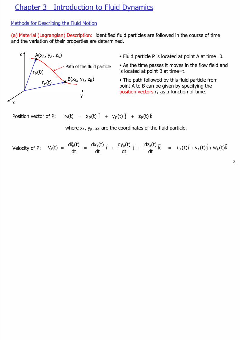
Chapter 3 Introduction to Fluid Dynamics

Methods for Describing the Fluid Motion

(a) Material (Lagrangian) Description: identified fluid particles are followed in the course of timeand the variation of their properties are determined.

Path of the fluid particle

• The path followed by this fluid particle from

point A to B can be given by specifying theposition vectors rP as a function of time.

y

z

x

• Fluid particle P is located at point A at time=0.A(xA , yA , zA )

rP(0)

B(xB, yB, zB)rP(t)

• As the time passes it moves in the flow field andis located at point B at time=t.

k (t)z j (t)y i (t)x(t)r PPPP

rrr

r

++=Position vector of P:

where xP, yP, zP are the coordinates of the fluid particle.

k )t(wj)t(vi)t(u k dt(t)dz j

dt(t)dy i

dt(t)dx

dt(t)rd (t)V PPP

PPPPP

rrrrrr

r

r

++=++==Velocity of P:

2

8/7/2019 me305 chapter 3


Material (Lagrangian) Description (cont’d)

• In the Lagrangian description, coordinates of the fluid particle (xP, yP, zP) are dependent variables.

• They depend on time. They are used to locate the particle when the time is known.

] t ),t(z ),t(y ),t(x [ V V PPPPP

rr

=

] t ),t(z ),t(y ),t(x [ PPPPP ρ=ρ

etc.

• Fluid properties can be expressed as functions of xP, yP, zP and t, such as

Material Volume (Closed system): A collection of identified fluid particles.

• Its shape and position may change, but it contains always the same fluid particles.

• It is surrounded by the system boundaries, through which no particle can pass.

t = t0 t = t1 t = t2

3

8/7/2019 me305 chapter 3


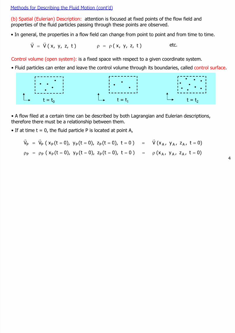
Methods for Describing the Fluid Motion (cont’d)

(b) Spatial (Eulerian) Description: attention is focused at fixed points of the flow field andproperties of the fluid particles passing through these points are observed.

) t ,z ,y ,x ( V Vrr

= ) t ,z ,y ,x ( ρ=ρ etc.

• In general, the properties in a flow field can change from point to point and from time to time.

Control volume (open system): is a fixed space with respect to a given coordinate system.

• Fluid particles can enter and leave the control volume through its boundaries, called control surface.

t = t0 t = t1 t = t2

• A flow filed at a certain time can be described by both Lagrangian and Eulerian descriptions,therefore there must be a relationship between them.

)0t ,z ,y ,x( V ) 0t ),0t(z ),0t(y ),0t(x ( V V A A A PPPPP =======rrr

)0t ,z ,y ,x( ) 0t ),0t(z ),0t(y ),0t(x ( A A A PPPPP =ρ=====ρ=ρ

• If at time t = 0, the fluid particle P is located at point A,

4

8/7/2019 me305 chapter 3


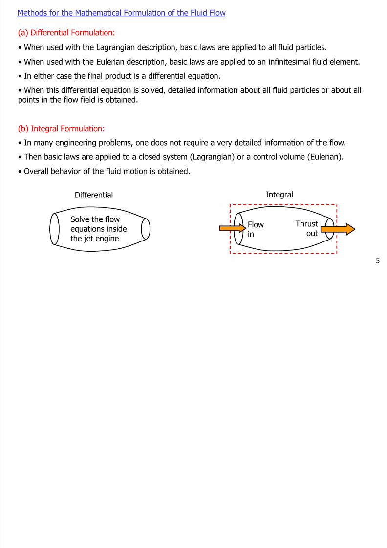
Methods for the Mathematical Formulation of the Fluid Flow

(a) Differential Formulation:

• When used with the Lagrangian description, basic laws are applied to all fluid particles.

• When used with the Eulerian description, basic laws are applied to an infinitesimal fluid element.

• In either case the final product is a differential equation.

• When this differential equation is solved, detailed information about all fluid particles or about allpoints in the flow field is obtained.

(b) Integral Formulation:

• In many engineering problems, one does not require a very detailed information of the flow.

• Then basic laws are applied to a closed system (Lagrangian) or a control volume (Eulerian).

• Overall behavior of the fluid motion is obtained.

Flow

in

Thrust

out

Integral

Solve the flow

equations insidethe jet engine

Differential

5

8/7/2019 me305 chapter 3


Relations Between the Material and Spatial Descriptions in the Differential Formulation

• One can relate the rate of change of any property of a fluid particle in the material description, tothe rate of chage of the same property in the spatial description at the point of the flow field where

the particle is located.

) t ,z(t) ),t(y ),t(x ( NN =• In material description any property N can be expressed as

dt t

N dz

z

N dy

y

N xd

x

N DN

∂

∂+

∂

∂+

∂

∂+

∂

∂=• Total differential of this property is

t

N

dt

dz

z

N

dt

dy

y

N

dt

xd

x

N

dt

DN

∂∂

+∂∂

+∂∂

+∂∂

=• Divide by dt

z N w

yN v

x N u

t N

dtDN

∂∂+

∂∂+

∂∂+

∂∂=• Use velocity components u, v and w

N )V( t

N

dt

DN∇⋅+

∂

∂=

rr• Put into vectorial notation

• D/dt represents the rate of change of a property in the material description. It is called the totalderivative, substantial derivative, material derivative or the derivative following the fluid.

• ∂ /∂t represents the rate of change of a property in the spatial description. It is called the partial

derivative, local derivative or the spatial derivative.• (V.∇) N represents the change of the property N from one point of the flow field to the other ata certain time. It is called the convective derivative (read details from the book).

6

8/7/2019 me305 chapter 3


Relations Between the Material and Spatial Descriptions in the Integral Formulation

(Reynold’s Transport Theorem)

• To relate the change of any extensive property N of a closed system to the variations of the sameproperty associated with the control volume, consider the case shown below.

• Initially (at time t0), the system boundary coincides with the boundary of the control volume (CV).

• After a time interval of ∆t (at time t0+∆t), the control volume remains in its original position,however the system moves to a new position.

• The mass in region A enters into the CV, while the mass in region C leaves the CV.

• Details of the derivation of Reynold’s Transport Theorem will be given during the class.

system

control

volume

time t0 + ∆t

A

C

B

system

time t0

flow fieldcontrolvolume

7

8/7/2019 me305 chapter 3


3.5 Classification of Fluid Flow

Steady and Unsteady Flows:

• The flow is referred as steady when the properties of the flow field are independent of time.

etc. , )z,y,x( , )z,y,x(pp , )z,y,x(VV ρ=ρ==rr

• In a steady flow, properties of the flow field are functions of the space coordinates.

etc. , 0t

, 0t

p , 0

t

Vor =

∂ρ∂

=∂∂

=∂∂r

• In an unsteady flow, one or more properties change with time.

• Whether the flow is steady or not depends on the choice of the coordinate system with whichthe motion is observed.

• An unsteady flow relative to a stationary reference frame can be simplified to a steady flow if analyzed from a moving reference frame.

Movie Time:

8

8/7/2019 me305 chapter 3


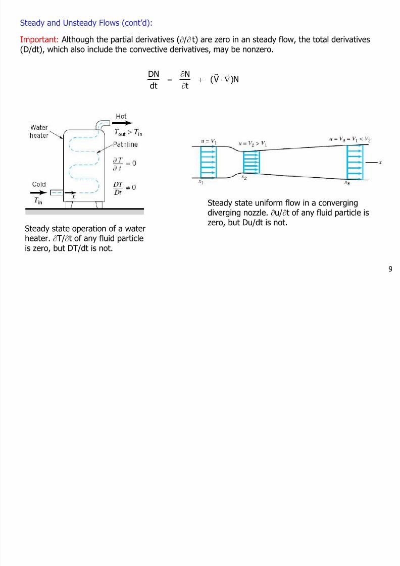
Steady and Unsteady Flows (cont’d):

Important: Although the partial derivatives (∂/∂ t) are zero in an steady flow, the total derivatives

(D/dt), which also include the convective derivatives, may be nonzero.

N)V( t

N

dt

DN∇⋅+

∂

∂=

rr

Steady state operation of a water

heater. ∂T/∂t of any fluid particleis zero, but DT/dt is not.

Steady state uniform flow in a convergingdiverging nozzle. ∂u/∂t of any fluid particle iszero, but Du/dt is not.

9

8/7/2019 me305 chapter 3


Three- , Two- and One-Dimensional Flows:

Three-dimensional flow:

• Generally a fluid flow is a rather complex three-dimensional phenemenon.

• Fluid properties vary in all three mutually perpendicular directions.

t)z,y,(x, , t)z,y,p(x,p , )t,z,y,x(ww , )t,z,y,x(vv, )t,z,y,x(uu ρ=ρ====

• For example in the Cartesian coordinate system

Flow visualization of the complex

three-dimensional flow field pasta model airfoil.

Movie Time:

• Even in the most simple flows, velocity field generally has all three components nonzero.

• But still, dependence of the fluid properties in one or two directions might be small compared tothe other direction(s).

• In these cases the flow can be simplified as being two- or even one-dimensional.

10

8/7/2019 me305 chapter 3


Two-dimensional flow: Properties are functions of time and two space coordinates (say x and y).

t)y,(x, , t)y,p(x,p , )t,y,x(ww , )t,y,x(vv, )t,y,x(uu ρ=ρ====

• Variation of the properties in the third direction (z) is assumed to be negligible.

x

y

constant , p(x)p

0w , 0v, )y,x(uu

=ρ=

===

Two-dimensional flow between twodiverging plates.

11

8/7/2019 me305 chapter 3


One-dimensional flow: Fluid properties are functions of time and one space coordinate (say x).

t)(x, , t)p(x,p , )t,x(ww , )t,x(vv, )t,x(uu ρ=ρ====

constant ,constantp

0w , 0v, )y(uu

=ρ=

===

Uniform flow: For the sake of simplicity, the properties at a cross-section can be approximated byits average values.

• Then the properties are said to be uniform over that cross-section.

Uniform one-dimensional flowin a constant diameter pipe.

Uniform one-dimensional flowbetween two diverging plates.

12

3 6 Vi li i f h Fl id Fl

8/7/2019 me305 chapter 3


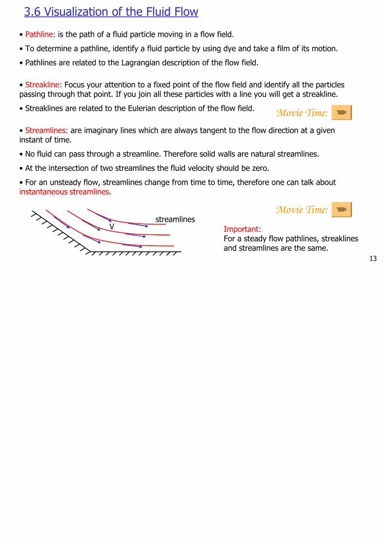
3.6 Visualization of the Fluid Flow

• Pathline: is the path of a fluid particle moving in a flow field.

• To determine a pathline, identify a fluid particle by using dye and take a film of its motion.

• Pathlines are related to the Lagrangian description of the flow field.

• Streakline: Focus your attention to a fixed point of the flow field and identify all the particles

passing through that point. If you join all these particles with a line you will get a streakline.

• Streaklines are related to the Eulerian description of the flow field.

• Streamlines: are imaginary lines which are always tangent to the flow direction at a given

instant of time.

• No fluid can pass through a streamline. Therefore solid walls are natural streamlines.

• At the intersection of two streamlines the fluid velocity should be zero.

• For an unsteady flow, streamlines change from time to time, therefore one can talk aboutinstantaneous streamlines.

Movie Time:

Movie Time:streamlines

VImportant:For a steady flow pathlines, streaklinesand streamlines are the same.

13

8/7/2019 me305 chapter 3


Derivation of a streamline:

• After an infinitesimal time interval, the particle will move to adifferent location.

r+dr

instantaneousstreamline

• Consider a fluid particle with a position vector r at a certain

time.

y

z

x

r

drV

• During this infinitesimal time interval, the position change of

the particle, dr, coincides with the instantaneous streamline.

• That is, the velocity vector V = u i + v j + w k is parallel to dr = dx i + dy j + dz k .

w

dz

v

dy

u

dx ==• In other words V x dr = 0. This gives the equation of a streamline as

14

Streamtube: is formed by a bundle of streamlines passing

through a closed curve in space. streamlines• For a steady flow, streamtube behaves like a real tube,because no particles can pass through the boundaries of astreamtube (they are formed by streamlines).

• For an unsteady flow, streamtube changes its position fromtime to time and the fluid particles that form the streamtubechange with time.

8/7/2019 me305 chapter 3


Example:

• The velocity field for a fluid flow is given as

V = 2x i – 2y j (m/s).

(a) Determine whether the flow field is three-, two- or one-dimensional.

(b) Determine the components of the velocity vector at point P(2,2,0).

(c) Determine the magnitude and direction of the velocity vector at point P.

(d) Determine the equation of the streamline passing through point P.(e) Sketch the velocity vector and the streamline.

Solution will be given during the class.

15

3 7 Accele ation of a Fl id Pa ticle

8/7/2019 me305 chapter 3


3.7 Acceleration of a Fluid Particle

dt

VD

a

r

r

= V)V(t

V

rrr

r

∇⋅+∂

∂

=

• ∂V/∂t is the local acceleration.

• (V .∇)V is the convective acceleration.

• This is a vector equation and can be expressed in the Cartesian coordinate system as follows

k a ja ia a zyx

rrr

v

++= k dt

Dw j

dt

Dv i

dt

Du

dt

VD

rrr

r

++==

• or in more detail

z

uw

y

uv

x

uu

t

u )uV(

t

u

dt

Du ax ∂

∂+

∂∂

+∂∂

+∂∂

=∇⋅+∂∂

==rr

z

vw

y

vv

x

vu

t

v )vV(

t

v

dt

Dv ay ∂

∂+

∂

∂+

∂

∂+

∂

∂=∇⋅+

∂

∂==

rr

z

ww y

wv x

wu t

w )wV( t

w dt

Dw az ∂

∂+∂

∂+∂

∂+∂

∂=∇⋅+∂

∂==

rr

16

8/7/2019 me305 chapter 3


Acceleration vector in the cylindrical coordinate system:

z z r r ia ia ia arrr

v

++= θθ

• or in more detail

r

V -

z

VV

V

r

V

r

VV

t

V a

2r

zrr

rr

rθθ ∂

∂∂+

θ∂∂+

∂∂+

∂∂=

r

VV

z

VV

V

r

V

r

VV

t

V a r

zrθθθθθθ

θ +

∂

∂+

θ∂

∂+

∂

∂+

∂

∂=

z

VV

V

r

V

r

VV

t

V a r

zzz

rz

z ∂∂

+θ∂

∂+

∂∂

+∂

∂= θ

• Think about where the additional terms are coming from.

• Similarly acceleration components in the spherical coordinate system () can be written.

17

8/7/2019 me305 chapter 3


Example:

• A velocity field is given as

V = x2 i – 2xyt j + 3z k (m/s).

(a) Determine the acceleration field a .

(b) Determine the acceleration at point P(1,2,3) and time t=10 s.


18

8/7/2019 me305 chapter 3


Example:

• Consider one-dimensional, steady, incompressible flow through a converging channel.

• The velocity field is given by V = Uo (1 + x/L ) i

(a) Determine the acceleration field a by using the Eulerian method.

(b) Using the Lagrangian method, determine the equations for the position and acceleration of a

fluid particle as a function of time, which is located at x = 0 at time t = 0.

(c) Show that both expressions for the acceleration give identical results, as this fluid particlepasses through the point at x = L.


x

y

L

19

3 8 Flow Rates and Average Velocity

8/7/2019 me305 chapter 3


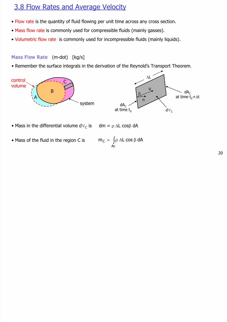
3.8 Flow Rates and Average Velocity

• Flow rate is the quantity of fluid flowing per unit time across any cross section.

• Mass flow rate is commonly used for compressible fluids (mainly gasses).

• Volumetric flow rate is commonly used for incompressible fluids (mainly liquids).

Mass Flow Rate (m-dot) [kg/s]

system

controlvolume C

A

B

• Remember the surface integrals in the derivation of the Reynold’s Transport Theorem.

∆L

dA C

at time t0 d∀C

dA Cat time t0+∆t

n

Vβ

• Mass in the differential volume d∀C is dm = ρ ∆L cosβ dA

∫ β∆ρ=Ac

C dA cosL m• Mass of the fluid in the region C is

20

8/7/2019 me305 chapter 3


Mass Flow Rate (cont’d)

• The mass flow rate going out of the control volume is

∆ t

mlim m c

0∆ t→=& ∫ →

=A

0∆ tβ dA cos

∆ t

∆ Lρ lim ∫ =

A

β dA cosρ V ∫ ⋅=A

dA nVρ rr

• Note that the mass in region C flows out through the control surface. Therefore the angle β isalways less than 90o and cosβ is always positive.

• Sign convention for mass flow rate:

• m-dot is positive if the mass goes out of the control volume.

• m-dot is negative if the mass goes into the control volume.

• Note that m-dot can be zero if either V or cos β is zero.

• For incompressible and uniform flow going out of a control volume m-dot = ρ A V

V

n

V

n

V

n

V

n

21

Volumetric Flow Rate (Q) [m3/s]

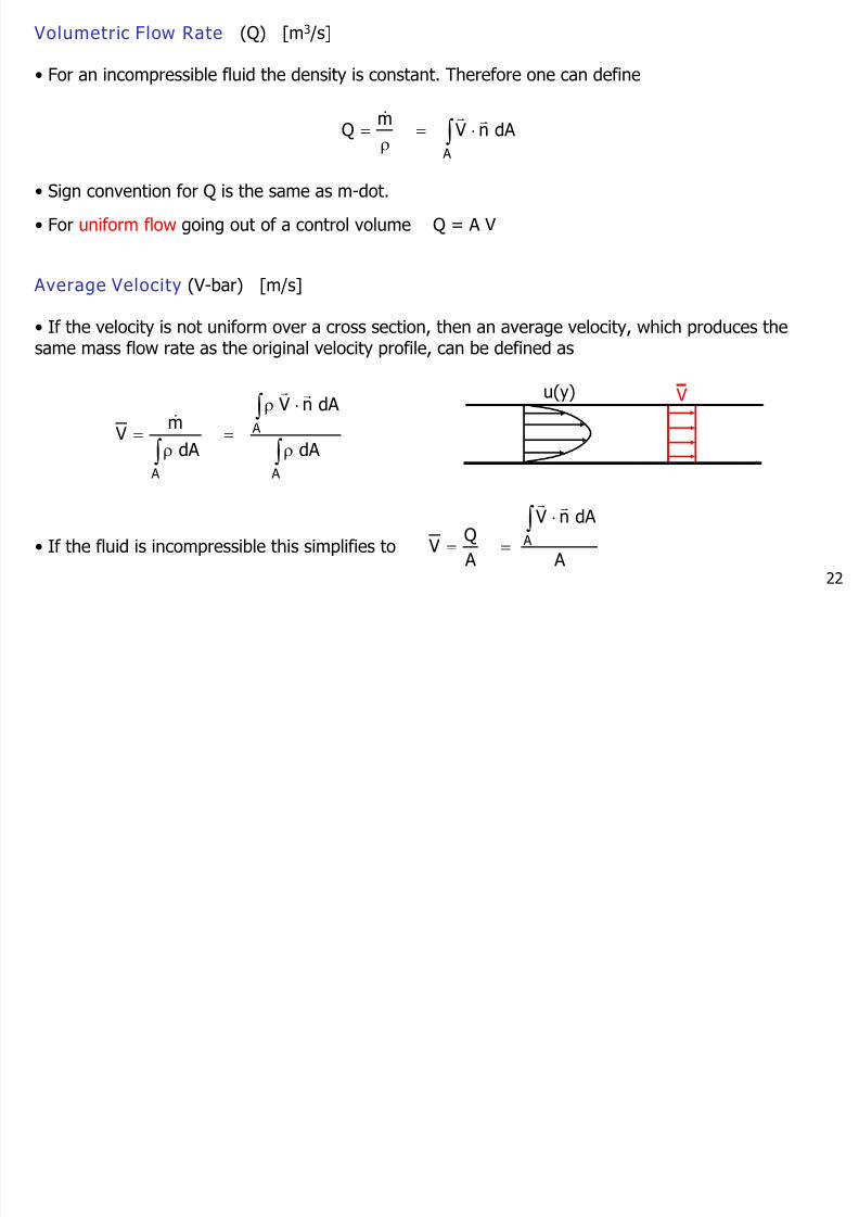
8/7/2019 me305 chapter 3


Volumetric Flow Rate (Q) [m3/s]

• For an incompressible fluid the density is constant. Therefore one can define

∫ ⋅=ρ

=A

dA nV m

Qrr&

• Sign convention for Q is the same as m-dot.

• For uniform flow going out of a control volume Q = A V

Average Velocity (V-bar) [m/s]

• If the velocity is not uniform over a cross section, then an average velocity, which produces thesame mass flow rate as the original velocity profile, can be defined as

∫ ∫

∫ ρ

⋅ρ

=ρ

=

A

A

A

dA

dA nV

dA

mV

rr

&

u(y) V

• If the fluid is incompressible this simplifies toA

dA nV

A

QV A ∫ ⋅

==

rr

22

Example 3 4

8/7/2019 me305 chapter 3


Example 3.4

Water with a density of 1000 kg/m3 is flowing through a pipe. The velocity of water, which is assumedto be uniform at the exit of the pipe, is 3 m/s. If the area at the exit is 0.001 m2, determine the mass

flow rate and the volumetric flow rate.

Flow

Vn

x

y

β=60o

Problem 3 .13

A viscous and incompressible fluid with a density of ρ is flowing through a wide flat channel with aheignt of 2h. At a certain section of the channel, the velocity distribution is given by u =UC [1-(y/h)2],where UC is the centerline velocity. Determine the mass flow rate per unit width, volumetric flow rate

per unit width and the average velocity.

u(y)

x

yh

h

23

bl 3

8/7/2019 me305 chapter 3


Problem 3 .14

A viscous and incompressible fluid with a density of ρ is flowing through a pipe with a radius of R. Thevelocity distribution in the pipe is given by Vx =UC [1-(r/R)], where UC is the centerline velocity.

Determine the mass flow rate, volumetric flow rate and the average velocity.

Vx(r)

x

r

R

24

me305 chapter 3

Documents