Mdl 4Module 4 2D Fourier Transformcoecs.ou.edu/Joseph.P.Havlicek/ece5273/notes/Module-4JH.pdf · Mdl 4Module 4 2D Fourier Transform ... 0 1 = ... • Step 2: add up the dot products

M d l 4Module 42D Fourier Transform

• Fourier Transform BasicsFourier Transform Basics

• Sinusoidal Image

2D Di F i T f• 2D Discrete Fourier Transform

• Meaning of Image Frequencies

• Sampling Theorem

• Some Important 2D DFT Pairs

1

Some Important 2D DFT Pairs

Joseph FourierJoseph Fourier

Y d 21 bi hd hYesterday was my 21st birthday, at that age Newton and Pascal had already acquired many claims to immortality. - In a letter by Fourier

• Fourier was a math professor. He studied heat conduction. His PhD advisor was Lagrange.g g• His most important contribution was

development of the idea that an arbitrary function could be written as an infinite sum (series) of sines and cosines.• Ironically, this work was bitterly

d b b h l dcriticized by both Laplace and Lagrange at the time!

2

Vectors in 2Vectors in • The natural basis:

R t ti it bit t

23

=

vy 2 { , }i jv• Representation: write an arbitrary vector

as a linear combination of the basis.

• Question: how do we do this?

v

• Answer: use the dot product (inner product).

• For two vectors and

, the dot product is often

01

=

j x [ ]1 2Tv v=v

[ ]1 2Tw w=w

written using angle brackets:10

=

i

[ ]

1 1 2 2, v w v w= +v w

• Recall that the dot product is a scalar.

• Any arbitrary can be written as 2∈v , , .= +v v i i v j j

3

y y , , j j

• For example, on the last page we had Using the dot product,[ ]2 3 .T=v

i i j j, ,

2 1 1 2 0 0, ,

3 0 0 3 1 1

= +

= +

v v i i v j j

( ) ( )

3 0 0 3 1 1

1 0 22 1 3 0 2 0 3 1

0 1 3

= ⋅ + ⋅ + ⋅ + ⋅ =

• This is a powerful way to think about things because it works for anyorthonormal basis.

• Fact: another orthonormal basis for 2 is given by the vectors

1 1T

= e 1 1T

− = e

• For , you can easily check that

1 2 2 = e 2 2 2

= e

[ ]2 3 T=v

4

1 1 1 12 2 2 2

1 1 2 2 1 1 1 12 2 2 2

2 2 2, , , ,

3 3 3

− − + = + =

v e e v e e

Some Important Things About the Dot Product

• In higher dimensional spaces like 100, it becomes convenient to useIn higher dimensional spaces like , it becomes convenient to use “Capital Sigma” notation to write the dot product:

100

1 1 2 2 100 100, k kv w v w v w v w= + + + =v w

• But the whole procedure still works exactly like before in 2.

• For an orthonormal basis , the representation of is

1k =

{ }1 2 100, , ,e e e v

• The operation of computing the dot products defines a

100

1 1 2 2 100 1001

, , , , k kk =

= + + + =v v e e v e e v e e v e e

, kv ep p g ptransform. It gives the representation (or coordinates) of relative to the basis .

• The operation of writing as sum of the basis vectors defines an

, k

v{ }1 2 100, , ,e e e

v

5

inverse transform.

Important Things About Dot ProductsImportant Things About Dot Products

• One thing you may not have been taught about the dot product is: if the vectors have complex entries, then you must conjugate one of the vectors in the dot product.

• In engineering, we always conjugate the second vector.

• The dot product then becomes*, k k

kv w=v w

• To write a vector as a sum of the basis, you still add up the dot products times the basis vectors just like before:

v

• Note: sometimes in math and physics, it is the first vector that gets j t d i th d t d t B t i i i l

, k kk

=v v e e

6

conjugated in the dot product. But in engineering, we alwaysconjugate the second vector.

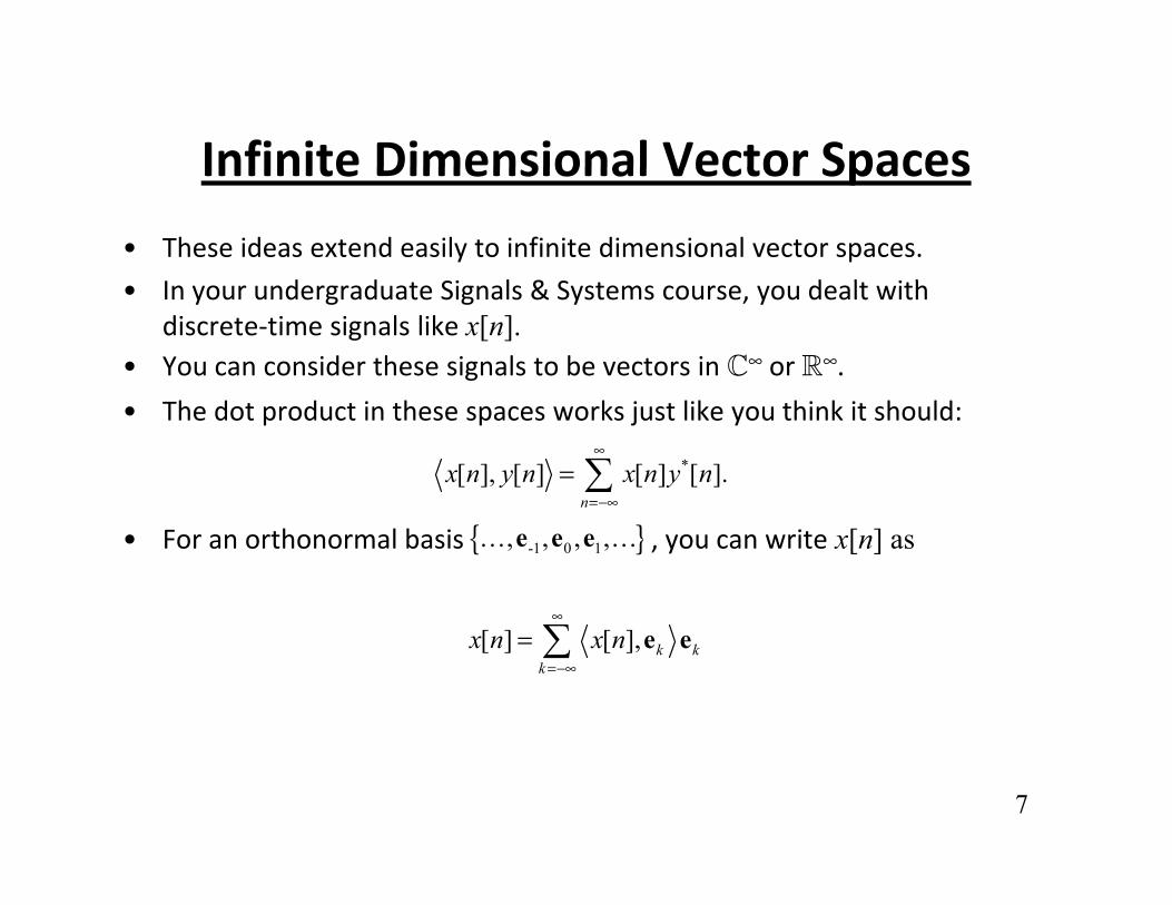
Infinite Dimensional Vector SpacesInfinite Dimensional Vector Spaces

• These ideas extend easily to infinite dimensional vector spaces.

I d d Si l & S d l i h• In your undergraduate Signals & Systems course, you dealt with discrete-time signals like x[n].

• You can consider these signals to be vectors in ∞ or ∞.

• The dot product in these spaces works just like you think it should:

*[ ], [ ] [ ] [ ].n

x n y n x n y n∞

=−∞

= • For an orthonormal basis , you can write x[n] as{ }-1 0 1, , , ,e e e

∞

[ ] [ ], k kk

x n x n=−∞

= e e

7

Natural Basis in ∞ or ∞Natural Basis in or • Think of the signals δ[n], δ[n-1], δ[n+1], and δ[n-k] from your

undergraduate Signals & systems courseundergraduate Signals & systems course.

• Each one of them is “turned on” in exactly one place where it is equal to one.

F f di i i l [ ] h f l• For vector spaces of discrete-time signals x[n], the set of translatesδ[n-k] of the Kronecker delta for k ∈ plays the same role that the basis plays in 2; i.e., it is the natural basis.

Th d d f [ ] i h h b i δ[ k] i h b

,{ }i j

• The dot product of x[n] with the basis vector δ[n-k] is the number

[ ], [ ] [ ] [ ] [ ].n

x n n k x n n k x kδ δ∞

=−∞

− = − =• The signal x[n] can be written as a sum of the basis just like before:

[ ] [ 1] [ 1] [0] [ ] [1] [ 1]x n x n x n x nδ δ δ∞ ∞

= + − + + + − +

8

[ ] [ ] [ ], [ ] [ ].k k

x k n k x n n k n kδ δ δ=−∞ =−∞

= − = − −

Uncountably Infinite DimensionsUncountably Infinite Dimensions

• We can let the number of dimensions grow even larger, so that it is equal to the number of real numbers in equal to the number of real numbers in .

• The vectors in these spaces are exactly the continuous-time signals x(t) from your undergraduate Signals & Systems course.E hi ill k j lik i did b f b h• Everything still works just like it did before, but now you have to use “Capital S” adding instead of “Capital Sigma” adding.

• The dot product in these spaces is given by

• For an orthonormal basis , you can write x(t) just like before:

*( ), ( ) ( ) ( ) .x t y t x t y t dt∞

−∞=

{ }τ τ∈e y ( ) j{ }τ τ∈

( ) ( ),x t x dτ ττ τ∞

−∞= e e

9

Uncountably Infinite DimensionsUncountably Infinite Dimensions• The natural basis is a little bit harder to talk about in this case,

because distribution theory is required to treat the Dirac delta δ(t)( )rigorously.

• Here, “distribution theory” means the theory of generalized functions. It has nothing to do with “probability distributions.”

• We won’t go into the details (take ECE 5213, DSP, for that).

• Nevertheless, it should make intuitive sense to you at this point that the natural basis is given by the translates of the Dirac delta:t e atu a bas s s g e by t e t a s ates o t e ac de ta:

• The dot product of x(t) with a basis function is the number

{ }( )t τδ τ∈

−

• You write x(t) as a sum of the basis just like before, by adding up the dot products times the basis vectors:

( ), ( ) ( ) ( ) ( ).x t t x t t dt xδ τ δ τ τ∞

−∞− = − =

10

p

( ) ( ) ( ) .τ δ τ τ∞

−∞= −x t x t d

Change of BasisChange of Basis• Recall from calculus that changing coordinate systems can sometimes

turn a hard problem into an easier one.

– For example, when computing a solid of revolution, switching from rectangular coordinates to cylindrical coordinates often makes the problem easier.

• Similarly, when working on signals or images, it is sometimes very useful to change from the natural basis to some other basis.

• This can let you look at the signal in a different way where it’s easier s ca et you oo at t e s g a a d e e t ay e e t s eas eto see different information that might be important for a particular problem.

• It can also turn some “hard” problems into easy ones. For example, p y p ,an appropriate change of basis turns convolution into multiplication (more on this later).

11

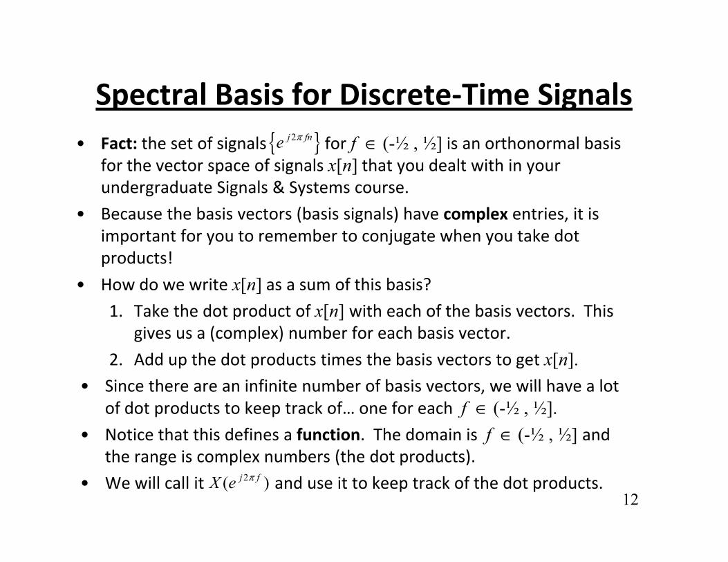
Spectral Basis for Discrete-Time SignalsSpectral Basis for Discrete Time Signals• Fact: the set of signals for f ∈ (-½ , ½] is an orthonormal basis

for the vector space of signals x[n] that you dealt with in your { }2j fne π

undergraduate Signals & Systems course.

• Because the basis vectors (basis signals) have complex entries, it is important for you to remember to conjugate when you take dot products!

• How do we write x[n] as a sum of this basis?

1. Take the dot product of x[n] with each of the basis vectors. This1. Take the dot product of x[n] with each of the basis vectors. This gives us a (complex) number for each basis vector.

2. Add up the dot products times the basis vectors to get x[n].• Since there are an infinite number of basis vectors we will have a lot• Since there are an infinite number of basis vectors, we will have a lot

of dot products to keep track of… one for each f ∈ (-½ , ½].• Notice that this defines a function. The domain is f ∈ (-½ , ½] and

the range is complex numbers (the dot products)

12

the range is complex numbers (the dot products).

• We will call it and use it to keep track of the dot products.2( )j fX e π

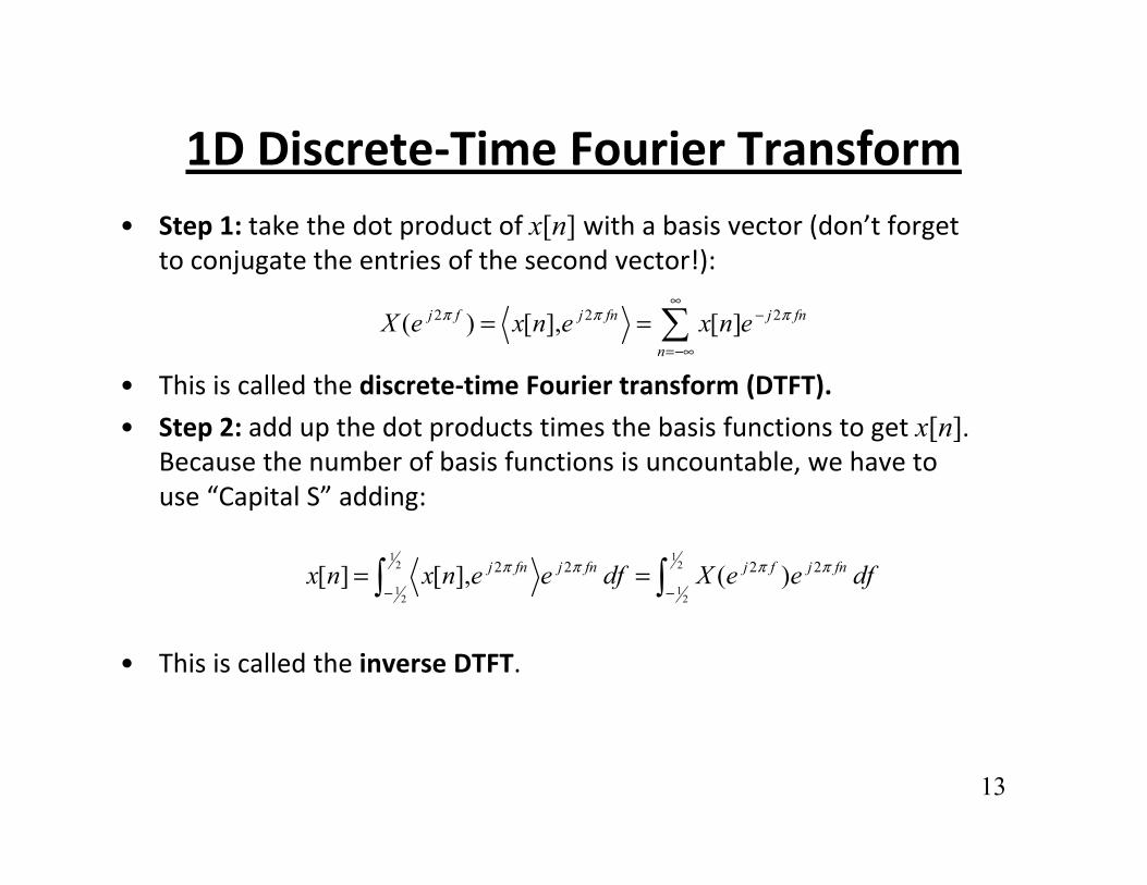
1D Discrete-Time Fourier Transform1D Discrete Time Fourier Transform• Step 1: take the dot product of x[n] with a basis vector (don’t forget

to conjugate the entries of the second vector!):

• This is called the discrete-time Fourier transform (DTFT)

2 2 2( ) [ ], [ ]j f j fn j fn

nX e x n e x n eπ π π

∞−

=−∞

= = • This is called the discrete-time Fourier transform (DTFT).

• Step 2: add up the dot products times the basis functions to get x[n].Because the number of basis functions is uncountable, we have to use “Capital S” adding:use Capital S adding:

1 12 2

1 12 2

2 2 2 2[ ] [ ], ( )j fn j fn j f j fnx n x n e e df X e e dfπ π π π− −

= =

• This is called the inverse DTFT.

13

Why Use the DTFT?Why Use the DTFT?• Looking at the graph of can make it easy to see certain things

that are hard to see from the graph of x[n].2( )j fX e π

– For example, if x[n] is a digital audio signal, changing to the spectral basis and looking at the graph of may make it easy to see if there is too much bass or not enough midrange.

2( )j fX e π

• Let H be a discrete-time LTI system with impulse response h[n] and frequency response

• For an arbitrary input signal x[n], the output signal is given by the

2( ).j fH e π

For an arbitrary input signal x[n], the output signal is given by the convolution y[n] = x[n] * h[n] which can take a lot of work to compute.

• But if x[n] is an eigenfunction of the system, then the output is easy [ ] g y , p yto compute. It is given by y[n] = λ x[n], where λ is an eigenvalue that is complex-valued in general.

• For an arbitrary input signal x[n], the output will be easy to compute

14

y p g [ ], p y pif we can write x[n] as a sum of eigenfunctions. Each term of the sum will just get multiplied by a complex eigenvalue.

• Fact: the DTFT basis signals are all eigenfunctions of any discrete-time LTI system. The eigenvalues are given by the system frequency response.

• Proof: let the system input be The output is given by2[ ] .j fnx n e π=

[ ] [ ] [ ] [ ] [ ]y n x n h n x n k h k∞

= ∗ = −2 ( )

[ ] [ ] [ ] [ ] [ ]

[ ]

k

j f n k

k

y n x n h n x n k h k

e h kπ

=−∞

∞−

=−∞

= ∗ =

=

2 2 2[ ] ( ) [ ].j fn j fk j f

ke h k e H e x nπ π π

∞−

=−∞

= =

• Use the DTFT to write an arbitrary input x[n] as a sum of eigenfunctions. The system output is given by

{ }{ } { }{ }

12

12

12

12

2 2

2 2

[ ] [ ] ( )

( )

j f j fn

j f j fn

y n H x n H X e e df

X e H e df

π π

π π

−

−

= =

=

15

2

1 12 2

1 12 2

2 2 2 2 2( ) ( ) ( ) .j f j f j fn j f j fnX e H e e df Y e e dfπ π π π π− −

= =

• In other words, for an arbitrary input signal x[n], the output of the LTI system H is given by

• If we represent the input signal using the natural basis, then

{ }2 2[ ] IDTFT ( ) ( ) .j f j fy n X e H eπ π=

If we represent the input signal using the natural basis, then convolution is required to compute the system output.

• But if we use the DTFT to change to the spectral basis, then the output is given by multiplication.output is given by multiplication.

16

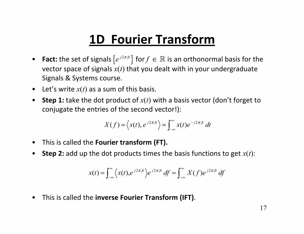
1D Fourier Transform1D Fourier Transform• Fact: the set of signals for f ∈ is an orthonormal basis for the

vector space of signals x(t) that you dealt with in your undergraduate { }2j fte π

( )Signals & Systems course.

• Let’s write x(t) as a sum of this basis.

• Step 1: take the dot product of x(t) with a basis vector (don’t forget toStep 1: take the dot product of x(t) with a basis vector (don t forget to conjugate the entries of the second vector!):

2 2( ) ( ), ( )j ft j ftX f x t e x t e dtπ π∞ −

−∞= =

• This is called the Fourier transform (FT).

• Step 2: add up the dot products times the basis functions to get x(t):

2 2 2( ) ( ), ( )j ft j ft j ftx t x t e e df X f e dfπ π π∞ ∞

−∞ −∞= =

17• This is called the inverse Fourier Transform (IFT).

Orthogonal BasisOrthogonal Basis• Going back to 2, consider the basis

[ ]T [ ]T

• This basis is orthogonal, but it is not orthonormal since each basis vector has length three instead of one

[ ]1 3 0 T=e [ ]2 0 3 T=e

vector has length three instead of one.

• If we try to write the vector as a sum of this basis using our method, we get

[ ]2 3 T=v

2 3 3 2 0 0

( ) ( )

1 1 2 2

2 3 3 2 0 0, , , ,

3 0 0 3 3 3

3 02 3 3 0 2 0 3 3

+ = +

= ⋅ + ⋅ + ⋅ + ⋅

v e e v e e

( ) ( )2 3 3 0 2 0 3 30 3

3 0 18 26 9 9

0 3 27 3

= ⋅ + ⋅ + ⋅ + ⋅

= + = =

18

• We get the wrong answer.

– Because the basis was not orthonormal, the dot products were all , ptoo big by a factor of 3.

– We multiplied these dot products that were all too big times basis vectors that were all too long by a factor of 3.g y

• All together, our answer is too big by a factor of 3×3 = 9, which is the length of a basis vector squared.

• When the basis is orthogonal but not orthonormal our method needsWhen the basis is orthogonal, but not orthonormal, our method needs some “fixing up.”

– We can divide by the squared length of a basis vector when we compute the dot products (fix up on the transform),compute the dot products (fix up on the transform),

– or we can divide by the squared length of a basis vector when we add up the dot products times the basis vectors (fix up on the inverse transform).inverse transform).

– or we can divide by the length of a basis vector in both places (fix up on both the transform and the inverse transform).

19

• You will often see the DTFT basis written in terms of radian frequency instead of Hertzian frequency.

• The basis is then for ω ∈ (-p , p].• This basis is orthogonal, but it is not orthonormal.

– Using the Riemann-Lebesgue lemma of distribution theory one

{ }j ne ω

Using the Riemann Lebesgue lemma of distribution theory, one can show that the length of each basis vector is not one (take ECE 5213, DSP, for the details).

– Because of this, we have to divide by 2p somewhere to make our

2 ,π

Because of this, we have to divide by 2p somewhere to make our method work.

• In engineering, the most common convention is to divide by 2p on the inverse transform. This gives the alternate DTFT/IDTFT definitioninverse transform. This gives the alternate DTFT/IDTFT definition

( ) [ ]j j n

nX e x n eω ω

∞−

=−∞

=

12[ ] ( )j j nx n X e e d

π ω ωππ ω

−=

20

which is found in many textbooks.

• Likewise, you will often see the FT basis written in terms of radian frequency instead of Hertzian frequency.

• The basis is then given by for ω ∈ .• This basis is again orthogonal but not orthonormal. Each basis vector

has length instead of one.

{ }j te ω

2πg

• This gives the alternate FT/IFT definition

j∞

( ) ( ) j tX x t e dtωω −

−∞=

12( ) ( ) j tx t X e dωπ ω ω

∞

−∞=

21

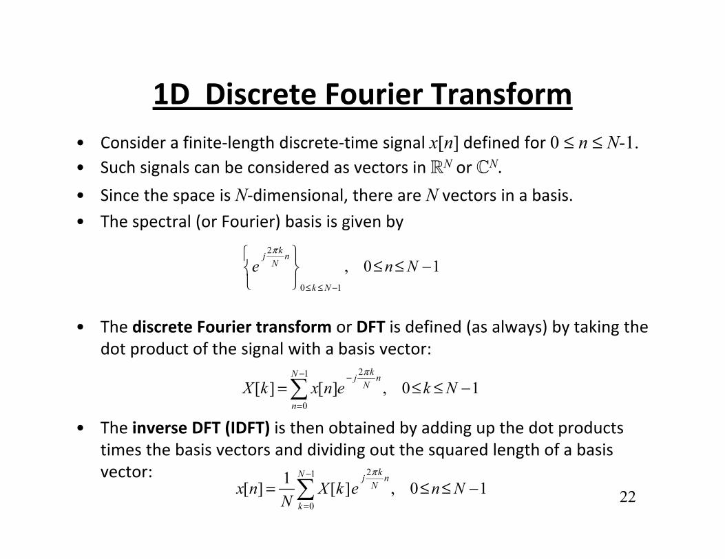
1D Discrete Fourier Transform1D Discrete Fourier Transform• Consider a finite-length discrete-time signal x[n] defined for 0 ≤ n ≤ N-1.• Such signals can be considered as vectors in N or N. g

• Since the space is N-dimensional, there are N vectors in a basis.

• The spectral (or Fourier) basis is given by2

0 1

, 0 1kj n

N

k N

e n Nπ

≤ ≤ −

≤ ≤ −

• The discrete Fourier transform or DFT is defined (as always) by taking the dot product of the signal with a basis vector:

21

[ ] [ ] 0 1kN j n

NX k k Nπ− −

≤ ≤• The inverse DFT (IDFT) is then obtained by adding up the dot products

times the basis vectors and dividing out the squared length of a basis

0[ ] [ ] , 0 1N

nX k x n e k N

=

= ≤ ≤ −

22

g q gvector: 21

0

1[ ] [ ] , 0 1kN j n

N

kx n X k e n N

N

π−

=

= ≤ ≤ −

• It is customary to write the DFT and IDFT using the shorthand notation 2 /j NW e π−=

• NOTE: WN is a complex number… a constant (for any fixed choice of N).

• The forward and reverse transforms then become

.NW e=

1

0[ ] [ ] , 0 1

Nkn

Nn

X k x n W k N−

=

= ≤ ≤ −

1N

• Notice that the conjugation operation is built in to the symbol W

1

0

1[ ] [ ] , 0 1N

knN

kx n X k W n N

N

−−

=

= ≤ ≤ −

• Notice that the conjugation operation is built in to the symbol WN.– This makes the “−” sign in the exponent appear on the inverse

transform instead of the forward transform when the “WN” notation is usedis used.

• Note: it’s important that the DFT math starts with n = 0 and k = 0.• In a Matlab DFT array, you have to remember that the first element has

i d 1 b t it’ f k 0

23

array index 1, but it’s for k = 0.

nD Sinusoids – Continuous CasenD Sinusoids Continuous Case• The 1D cosine:

• Instead of the scalar t in nD we have a position vector

cos(2 ).ftπ

[ ]Tx x x=x• Instead of the scalar t, in nD we have a position vector

• Instead of the scalar f, we have a frequency vector

• But the argument of cos must still be scalar.

h d d f h f d h

[ ]1 2 .nx x x=x [ ]1 2 .T

nu u u=u

• It is the dot product of the frequency vector and the position vector:

1 1 2 2T

n nu x u x u x= + + +u x

• The nD cosine:

• The nD sine:

• The nD complex exponential:

cos(2 ).Tπu xsin(2 ).Tπu x

2 cos(2 ) sin(2 )Tj T Te jπ π π= +u x u x u xThe nD complex exponential:

• Note: if n = 1, these reduce to the usual 1D definitions.

• We’ll develop intuition about them later; for now we focus on the math.

cos(2 ) sin(2 ).e jπ π= +u x u x

24

nD Fourier TransformnD Fourier Transform• For the nD continuous case, the spectral basis is• Let s(x) be an nD signal.

{ }2 .T

n

je π

∈

u x

u ( ) g

• For the FT, you simply take the dot product of s(x) with a basis signal (as always) – don’t forget to conjugate the entries of the second vector:

• You can “write out” the nD integral like this:

2( ) ( )T

n

jS s e dπ−= u xu x x

• The nD inverse Fourier Transform is just what you would expect:

( )1 1 2 221 2( ) ( ) n nj u x u x u x

nS s e dx dx dxπ∞ ∞ ∞ − + + +

−∞ −∞ −∞= u x

( )1 1 2 2221 2( ) ( ) ( )

Tn n

n

j u x u x u xjns S e d S e du du duππ ∞ ∞ ∞ + + +

−∞ −∞ −∞= = u xx u u u

25

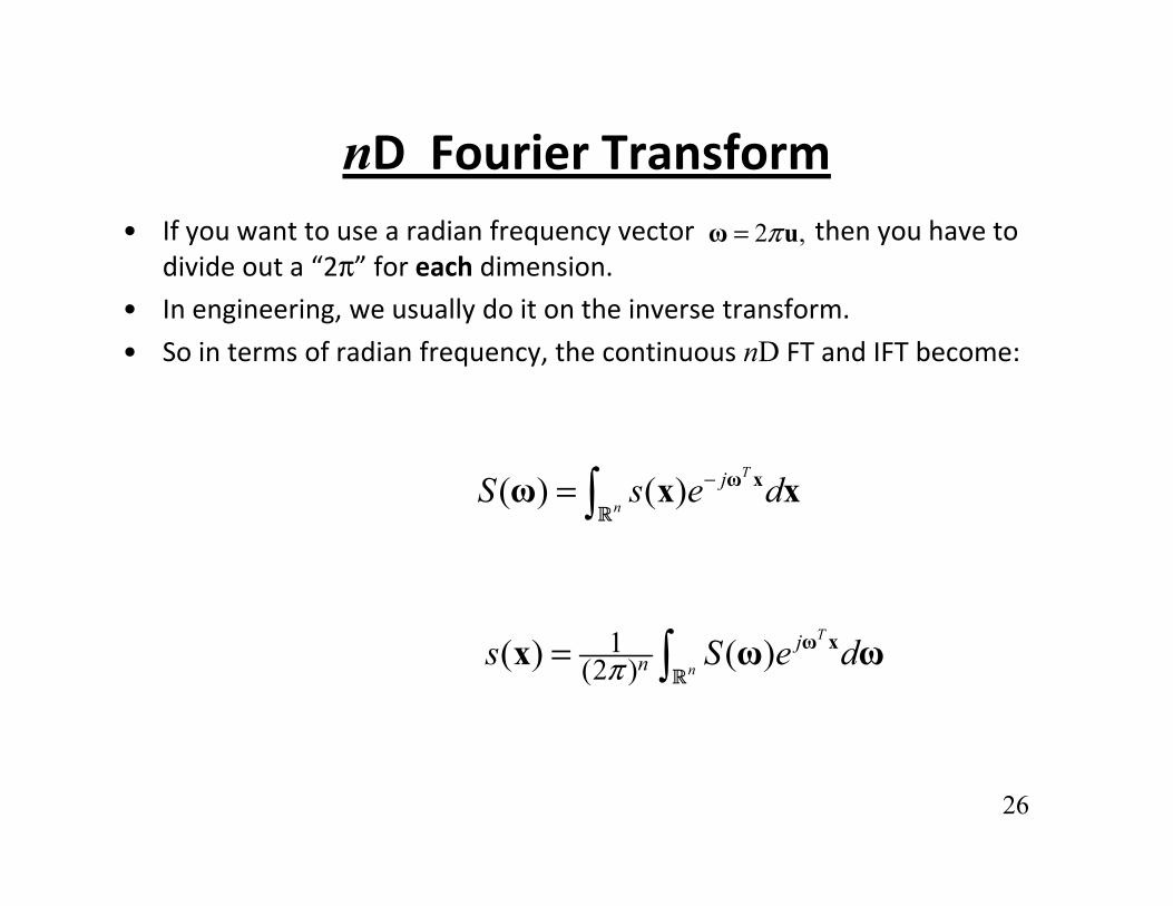
nD Fourier TransformnD Fourier Transform• If you want to use a radian frequency vector then you have to

divide out a “2π” for each dimension.2 ,π=ω u

• In engineering, we usually do it on the inverse transform.

• So in terms of radian frequency, the continuous nD FT and IFT become:

( ) ( )T

n

jS s e d−= ω xω x xn

1(2 )( ) ( )

T

n

jns S e dπ= ω xx ω ω

26

Important Notation ChangesImportant Notation Changes• For the rest of the module, we will write (m,n) for image

i l di F di i F i f hispatial coordinates. For discussing Fourier transforms, this almost always means (column, row).– Up to now we have thought of (m,n) as (row, col), consistent with p g ( , ) ( )

Matlab and usual matrix “row-col” addressing.

– But for the FT we think of 2D functions f(x,y), where x is horizontal.

• We will also usually think of the frequency in cycles per• We will also usually think of the frequency in cycles per image (cpi) instead of cycles per sample (pixel), since this is easier to interpret visually.

• For the case of 2D digital images, we will write the 2D frequency vector as where u = “horizontal frequency” and v = “vertical frequency.”

[ ] ,Tu v=u

27

frequency and v vertical frequency.

Sinusoidal Images

• We shall make frequent discussion in this d l f fmodule of image frequency content.

• The image having the simplest frequency content is the sinusoidal image.g

28

A di t i i I i i b

Sinusoidal Images

• A discrete sine image I is given by

( )I( ) sin 2 u vm n m nπ = +

and a discrete cosine image is given by

( )I( , ) sin 2 M Nm n m nπ = +

and a discrete cosine image is given by

( )I( , ) cos 2 u vM Nm n m nπ = +

for 0 ≤ m ≤ M-1, 0 ≤ n ≤ N-1

• Here, m is the column and n is the row.29

Important Note

• For the mathematics of the 2D Discrete Fourier Transform

Important Note

(DFT) to work out, it is very important that

– The first row in the image is row ZERO, not row one!

Th fi t l i l ZERO t l !– The first column is column ZERO, not column one!

• If the image is in a Matlab array, you must remember that the first row has index 1, but in terms of the mathematics, , ,it is row 0!

• Similarly, in a Matlab array, the first column has index 1, b t i t f th th ti it i l 0!but in terms of the mathematics it is column 0!

30

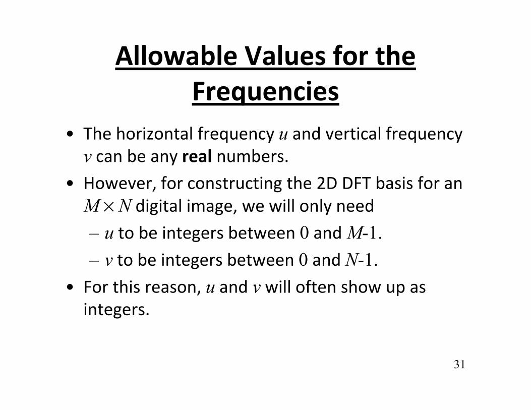
Allowable Values for the

h h i l f d i l f

Frequencies• The horizontal frequency u and vertical frequency

v can be any real numbers.

H f t ti th 2D DFT b i f• However, for constructing the 2D DFT basis for an M × N digital image, we will only need

u to be integers between 0 and M 1– u to be integers between 0 and M-1.– v to be integers between 0 and N-1.

F thi d ill ft h• For this reason, u and v will often show up as integers.

31

Cosine Images

• If M = N = 256, u = 4, and v = 0, then the image is

Cosine Images

I(m,n) = cos [2π m]4256

• Since the image does not depend on n every row isdepend on n, every row is the same.

• Every row is a cosine with 4 l icycles per image:

32

• If M = N = 256, u = 0, and v = 6, then the image isIf M N 256, u 0, and v 6, then the image is

I(m,n) = cos [2π n]6256

• Since the image does not depend on m, every column is the same.

• Every column is a cosine with 6 cycles per image:t 6 cyc es pe age

33

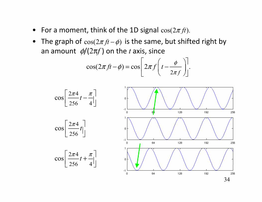
• For a moment, think of the 1D signal cos(2 ).ftπ• The graph of is the same, but shifted right by

an amount φ/(2πf ) on the t axis, sincecos(2 )ftπ φ−

φ 2

cos(2 ) cos 2 .f

ft f t φπ

π φ π − = −

2 4

256 4cos tπ π −

2 4

256cos tπ

2 4

256 4cos tπ π +

34

256 4

• Now, let M = N = 256, u = 4, and v = 6. The image isNow, let M N 256, u 4, and v 6. The image is

I(m,n) = cos [2π( m + n)]6256

O th fi t 0

4256

• On the first row, n=0, soI(m,n) = cos [2π m]

• On the 2nd row, n=1, so

4256

I(m,n) = cos [2π m + ]• On the 3rd row, n=2, so

I(m n) = cos [2π m + ]

4256

2 6256π

4256

2 12256πI(m,n) cos [2π m + ]

• On the kth row, n=k-1, soI(m,n) = cos [2π m + ]

Th ll i ith

256 256

4256

2 6( 1)256

kπ −

• They are all cosines with horizontal frequency 4 cpi.

• But each row is shifted by

35φ = compared to the row above.

2 6256π

• As an image, this looks like:( M = N = 256, u = 4, v = 6 )( M N 256, u 4, v 6 )

• Horizontally every row goes• Horizontally, every row goes through u=4 cycles across the image (but they start at different phase offsets).

• Vertically, every column y, ygoes through v=6 cycles down the image (but starting at different phase

36

starting at different phase offsets).

• If you take any horizontal slice through the image, you getIf you take any horizontal slice through the image, you get a 1D cosine with frequency u=4 cpi.

37

• If you take any vertical slice through the image, you get aIf you take any vertical slice through the image, you get a 1D cosine with frequency v=6 cpi.

38

• If you take a slice through the image in a direction normalIf you take a slice through the image in a direction normal to the wavefronts, you get a 1D cosine with frequency

cpi2 2 2 24 6 7.21u v+ = + =

Note: the main diagonal of the image is longer than one “image.” It has

39

Note: the main diagonal of the image is longer than one image. It hasa length of images. So along a line the length of the main diagonal, we expect to see about 1.41 × 7.21 = 10.17 cycles.

2 21 1 1.41+ =

Interpreting the 2D Frequencyu

Interpreting the 2D Frequency• The 2D frequency vector [u v]T has a

direction θ = tan-1(v/u)direction θ = tan 1(v/u).• This is usually called the frequency

orientation.

If d d h i h• If you draw u and v axes that agree with the sense of the image coordinates, then the frequency vector points in a direction normal to the wavefronts; it points in the

• The magnitude of the frequency vector isv

normal to the wavefronts; it points in the direction of “propagation.”

2 2Ω• This is called the radial frequency or magnitude frequency. It is also

often denoted by R.

2 2u vΩ = +

• In the direction θ, the frequency of oscillation is Ω cpi.

40

More on Cosine ImagesMore on Cosine Images

• If u = -4 and v = -6, we get the same image over again since cosine is even

u = -4; v = 6

cosine is even.

• However, the relative signs of , gu and v matter.

• If u = -4 and v = 6, it changes the orientation and we get a different image.

41

different image.

Sine Images• Everything works pretty much the same way for sine images.

• Except: since sine is odd if you negate both u and v it

Sine Images

• Except: since sine is odd, if you negate both u and v it multiplies the image by -1.

• Also, for a sine imageg

the pixel at m=0, n=0 is gray instead of white.

( )I( , ) sin 2 u vM Nm n m nπ = +

u=4, v=3 u=4, v=-3 u=-4, v=3 u=-4, v=-3

42

43Spatial Frequencies

Digital Sinusoid Example

• Let M = 16, v = 0: I(m) = cos(2πum/16): a cosine wave oriented in m-direction with frequency u. One row:

0

1u=1 or u=15

0

1u=2 or u=14

0

1u=4 or u=12

0

1u=8

1614121086420-1

0

i1614121086420-1

0

i1614121086420-1

0

i1614121086420-1

0

i

• Note that I(m) = cos (2πum/16) = cos [2π(16-u)m/16].• Thus the highest frequency wave occurs at u = M/2 (Mg q y (

is even here). This will be important later.44

Explanation• Why does cos(2πum/16) = cos[2π(16-u)m/16] ?

Th i th t ddi i t lti l f 2π t

p

• The reason is that adding any integer multiple of 2π to the argument of cos does not change the value.

( )2 2 2cos cosM u M um m mM M M

π π π− = − 2cos 2

M M M

u m mMπ π

= − +

2 2cos cos .u um mM Mπ π

= − =

45

• We’ll use complex exponential functions to define

Complex Exponential Image• We ll use complex exponential functions to define

the Discrete Fourier Transform.

• Define the 2-D complex exponential:

exp - 2 for 0 1, 0 1u vj m n m M n NM N

π + ≤ ≤ − ≤ ≤ −

• Here, we put the “-” sign in front of the j2π for b l h h Wcompatibility with the WN notation.

46

• Intuitively, the complex exponential image can be understood in terms of sine and cosine imagesunderstood in terms of sine and cosine images, since

exp - 2 cos 2 sin 2

2 i 2

u v u v u vj m n m n j m nM N M N M N

u v u v

π π π + = + − + − −

cos 2 sin 2 .u v u vm n j m nM N M N

π π = + + +

• Also note that the complex exponential image is separable:

- 2 - 2- 2u v vuj m n j nj mM N NM

π ππ +

47

M N NMe e e =

Properties of Complex ExponentialProperties of Complex Exponential

• Recall from page 4.23:

2W j π

(N = image dimension).

exp -NW jNπ =

( g )

• Hence, for a square image with M=N,

( )exp - 2 um vn um vnN NN

u vj m n W W WN N

π + + = =

48

• More generally, when the image is not square, we hhave

exp - 2 exp - 2 exp - 2u v u vj m n j m j nπ π π + = exp 2 exp 2 exp 2

um vnM N

j m n j m j nM N M N

W W

π π π+

=

• The magnitude and phase of the complex i l iexponential image are

exp - 2 1u vj m nπ + = exp 2 1

exp - 2 2

j m nM N

u v u vj m n m n

π

π π

+

∠ + = − +

49

exp 2 2j m n m nM N M N

π π∠ + = +

Complex Exponential ImageComplex Exponential Image

• From Euler's identity:• From Euler s identity:

2 2cos sinMW jπ π = − and

ium u u

M M Mj

cos 2 sin 2umM

u uW m j mM M

π π = −

• The u and v powers of WM and WN index the frequencies of the horizontal and vertical

50sinusoids.

Simple Properties of WM and WN

( )1cos 22

um vn um vnM N M N

u vm n W W W WM N

π − − + = +

( )1sin 22

um vn um vnM N M N

u vM N

m n j W W W Wπ − − + = −

2 2cos 2 sin 2 1umM

u uW m mπ π = + =

M M M

1tan sin 2 cos 2 2umM

uu uW m m mπ π π− ∠ = =

51

tan sin 2 cos 2 2MW m m mM M M

π π π∠

Comments

• It’s possible to develop frequency domain concepts without complex numbers - but the math is much lengthier.

• Using to represent a frequency componentll h ll d ll

um vnM NW W

oscillating horizontally at u cpi and vertically at v cpisimplifies things considerably.

It i f l t thi k f t tium vn• It is useful to think of as a representationof a direction and frequency of oscillation.

um vnM NW W

52

/Max/Min Values for u and v

• The complex exponential

( )2exp jumW umπ−=

is a sinusoid with frequency indexed by exponent u. • Minimum physical frequencies: u = kM k ∈

( )expM MW um=

• Minimum physical frequencies: u = kM, k ∈

0 1 ,m kMmM MW W m k= = ∀ ∈

• Maximum physical frequencies: u = (k+1/2)M (period 2)

( / 2) ( / 2)kM M M

53

( / 2) ( / 2)1 ( 1) ( even)kM M m M m mM MW W M+ = ⋅ = −

2D DISCRETE FOURIER TRANSFORM2D DISCRETE FOURIER TRANSFORM • Any M ´ N image I can be uniquely written as a weighted

f MN l i l b i isum of MN complex exponential basis images:

1 11I( , ) I( , ) (IDFT)M N

um vnM Nm n u v W W

− −− −=

• This is called the 2D Inverse Discrete Fourier

0 0I( , ) I( , ) (IDFT)M N

u vm n u v W W

MN = =

Transform or IDFT.

• The integers 0 ≤ u ≤ M-1 and 0 ≤ v ≤ N-1 index the basis images and give their frequencies in cpi.

• The weights are the 2D DFT coefficients of I.I

54

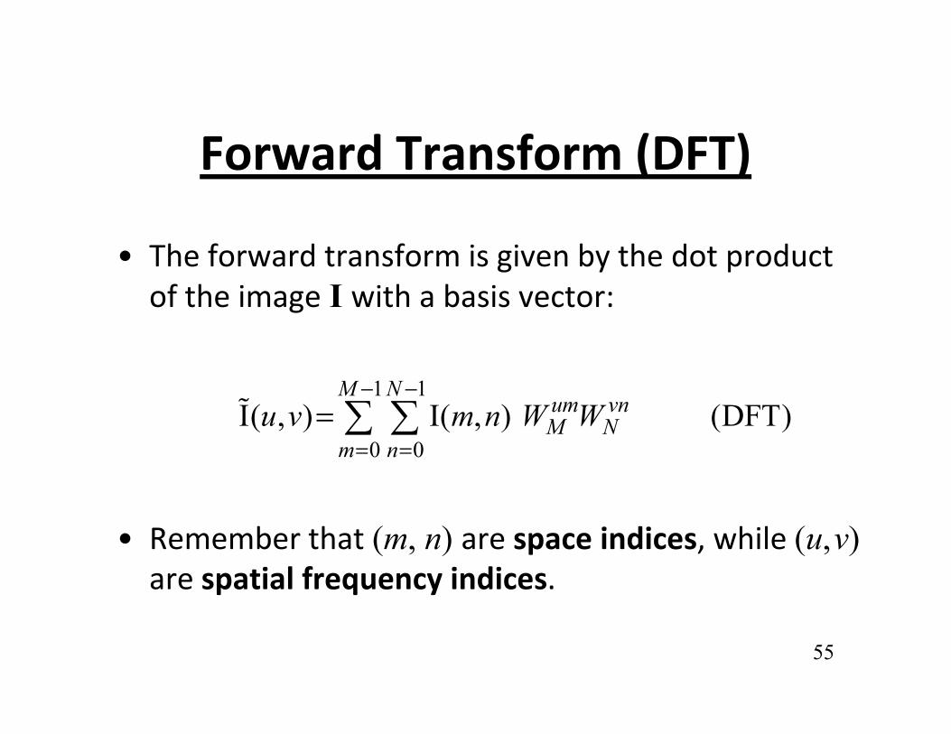
d f ( )Forward Transform (DFT)

• The forward transform is given by the dot product of the image I with a basis vector:

1 1I( ) I( ) (DFT)

M Num vnu v m n W W

− −

0 0I( , ) I( , ) (DFT)M N

m nu v m n W W

= ==

• Remember that (m, n) are space indices, while (u,v) are spatial frequency indices.

55

2D DFT as an Array2D DFT as an Array• The 2D DFT is an array with the same dimensions

(M ´ N) as the image I:

I( ); 0 1 0 1u v u M v N = ≤ ≤ − ≤ ≤ − I

• You can think of it as an image (complex-valued).

I( , ); 0 1, 0 1u v u M v N = ≤ ≤ − ≤ ≤ − I

• Note that the DFT is a linear transformation, so it commutes with linear combinations:

[ ]1 1 2 2 1 1 2 2DFT + +L L L La a a a a a+ ⋅ ⋅ ⋅ + = + ⋅ ⋅ ⋅ +I I I I I I

56

DFT Array Properties

• The DFT of an image I is generally complex:

l j= +I I I where

Real Imagj= +I I I

1 1M N 1 1

Real0 0

I ( , ) I( , )cos 2M N

m n

u vu v m n m nM N

π− −

= =

= +

1 1

Imag0 0

I ( , ) I( , )sin 2M N

m n

u vu v m n m nM N

π− − =− +

57

0 0m n M N= =

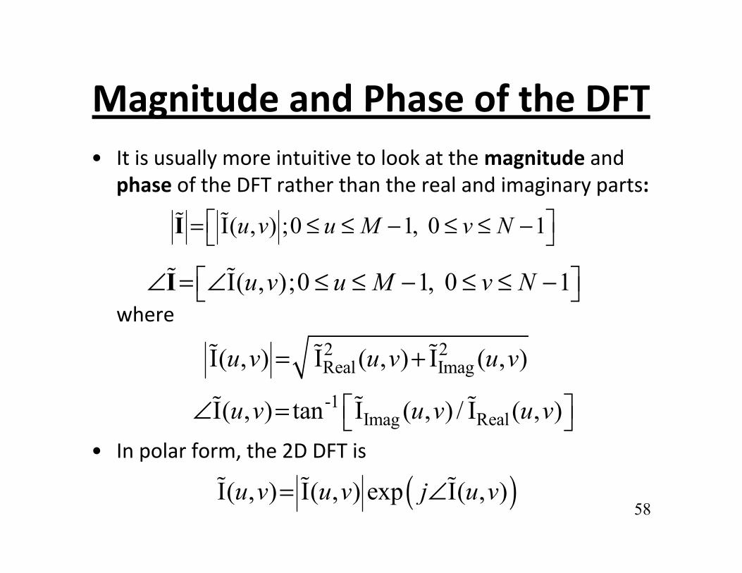
Magnitude and Phase of the DFTMagnitude and Phase of the DFT• It is usually more intuitive to look at the magnitude and

h f h DFT h h h l d i iphase of the DFT rather than the real and imaginary parts:

I( , ) ;0 1, 0 1u v u M v N = ≤ ≤ − ≤ ≤ − I

whereI( , );0 1, 0 1u v u M v N ∠ = ∠ ≤ ≤ − ≤ ≤ − I

2 2Real ImagI( , ) I ( , ) I ( , )u v u v u v= +

1

• In polar form, the 2D DFT is

-1Imag RealI( , ) tan I ( , ) / I ( , )u v u v u v ∠ =

58( )I( , ) I( , ) exp I( , )u v u v j u v= ∠

Symmetry of the DFTSymmetry of the DFT

• For a real image I, the DFT is conjugate symmetric:For a real image I, the DFT is conjugate symmetric:

*I( , ) I ( , ) ; 0 1, 0 1M u N v u v u M v N− − = ≤ ≤ − ≤ ≤ −

Proof:1 1

( ) ( )I( ) I( )M N

M u m N v nM u N v m n W W− −

− −= ( ) ( )

0 01 1

I( , ) I( , )

I( )

M Nm nM N

Mm um Nn vn

M u N v m n W W

W W W W

= =− −

− −

− − =

0 01 1 * *

I( , )

I( ) I ( )

Mm um Nn vnM M N N

m nM N

um vn

m n W W W W

W W

= =− −

=

590 0

I( , ) I ( , )um vnM N

m nm n W W u v

= = = =

More Symmetry PropertiesMore Symmetry Properties

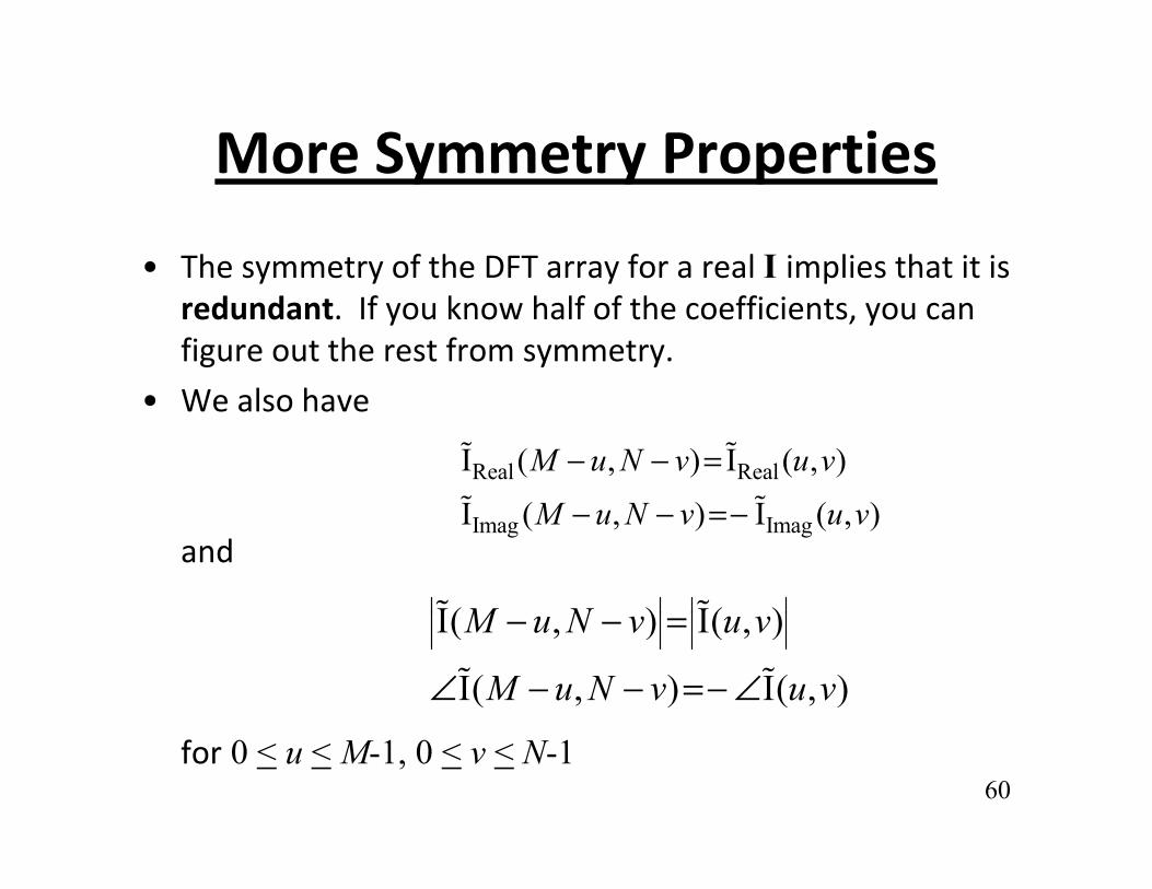
• The symmetry of the DFT array for a real I implies that it isThe symmetry of the DFT array for a real I implies that it is redundant. If you know half of the coefficients, you can figure out the rest from symmetry.

l h• We also have

Real RealI ( , ) I ( , )M u N v u v− − =

andImag ImagI ( , ) I ( , )M u N v u v− − =−

I( ) I( )M N I( , ) I( , )

I( , ) I( , )

M u N v u v

M u N v u v

− − =

∠ − − =− ∠

60for 0 < u < M-1, 0 < v < N-1

Viewing the DFT

• To view the DFT, we usually display the magnitude

Viewing the DFT

, y p y gand phase as images.

• In most cases, the phase is very difficult to interpret visually.

• Hence, it is common to look at the magnitude only.

• Logarithmic compression and a full-scale stretch are almost always applied to the magnitude for display:

log 1+ I( , )u v

• This is the log-magnitude spectrum of the image I.61

I ∠I

DC

62I ( )log 1+ I

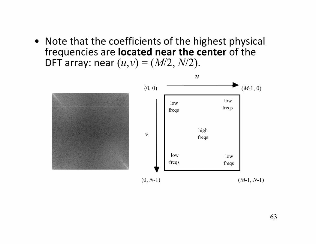
• Note that the coefficients of the highest physical g p yfrequencies are located near the center of the DFT array: near (u,v) = (M/2, N/2).

uu(0, 0)

low f

low

(M-1, 0)

v

freqsfreqs

high freqs

low freqs

low freqs

freqs

(0, N-1) (M-1, N-1)

63

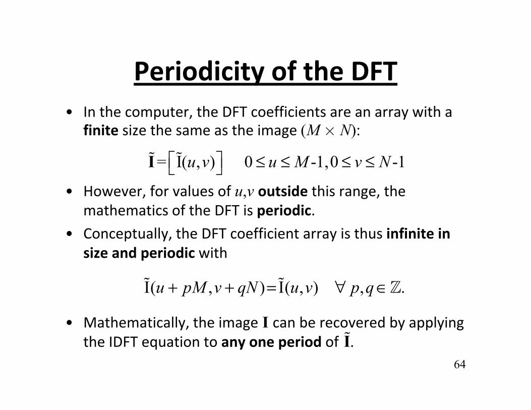
Periodicity of the DFTPeriodicity of the DFT• In the computer, the DFT coefficients are an array with a

finite i th th i (M ´ N)finite size the same as the image (M ´ N):

= I( , ) 0 -1,0 -1u v u M v N ≤ ≤ ≤ ≤ I

• However, for values of u,v outside this range, the mathematics of the DFT is periodic.

• Concept all the DFT coefficient arra is th s infinite in• Conceptually, the DFT coefficient array is thus infinite in size and periodic with

I( ) I( )M N ∀

• Mathematically, the image I can be recovered by applying

I( , ) I( , ) , .u pM v qN u v p q+ + = ∀ ∈

64

the IDFT equation to any one period of .I

Proof of DFT PeriodicityProof of DFT Periodicity• Let u,v be in the range 0 ≤ u ≤ M-1 and 0 ≤ v ≤ N-1.• Let p,q be any integers. Then

1 1M N− −1 1( ) ( )

0 01 1

I( , ) I( , ) M N

u pM m v qN nM N

m nM N

u pM v qN m n W W+ +

= =− −

+ + =

0 01 1

I( , ) um vn pMm qNnM N M N

m nM N

m n W W W W= =− −

=

0 0 I( , ) I( , )um vn

M Nm n

m n W W u v= =

= =

652 2 (int ) 1.

pMmjqMm j egerMMW e e

π π− −= = =This follows because

Periodically extended DFT array

(0,0)

66

Periodic Extension of ImagePeriodic Extension of Image• Mathematically, the DFT basis functions are defined

f ll i ll h i fi i i i d

um vnM NW W− −

for all integers m, n. Conceptually, they are infinite in size and periodic.

• When we write I as a sum of these basis functionsWhen we write I as a sum of these basis functions

1 1- -

0 0

1I( , ) I( , ) ,M N

um vnM Nm n u v W W

MN

− −=

it defines an image that is also infinite in size and periodic.

Th DFT d d d h f fi i i d

0 0u vMN = =

• The DFT does not understand the concept of a finite-sized image.

• To the mathematics of the DFT, every image is infinite in size

67

To the mathematics of the DFT, every image is infinite in size and periodic and every image has a DFT coefficient array that is also infinite in size and periodic.

Proof that the Image is PeriodicProof that the Image is Periodic

• Let m,n be in the range 0 ≤ m ≤ M-1 and 0 ≤ n ≤ N-1.• Let p,q be any integers. Then

1 1- ( ) - ( )

0 01 1

1I( , ) I( , )M N

u m pM v n qNM N

u vM N

m pM n qM u v W WMN

− −+ +

= =+ + =

1 1- - - -

0 01 1

1 I( , )

1

M Num vn upM vqN

M N M Nu vM N

u v W W W WMN

− −

= ==

1 1- -

0 0

1 I( , ) I( , )M N

Mm NnM N

u vu v W W m n

MN

− −

= == =

68

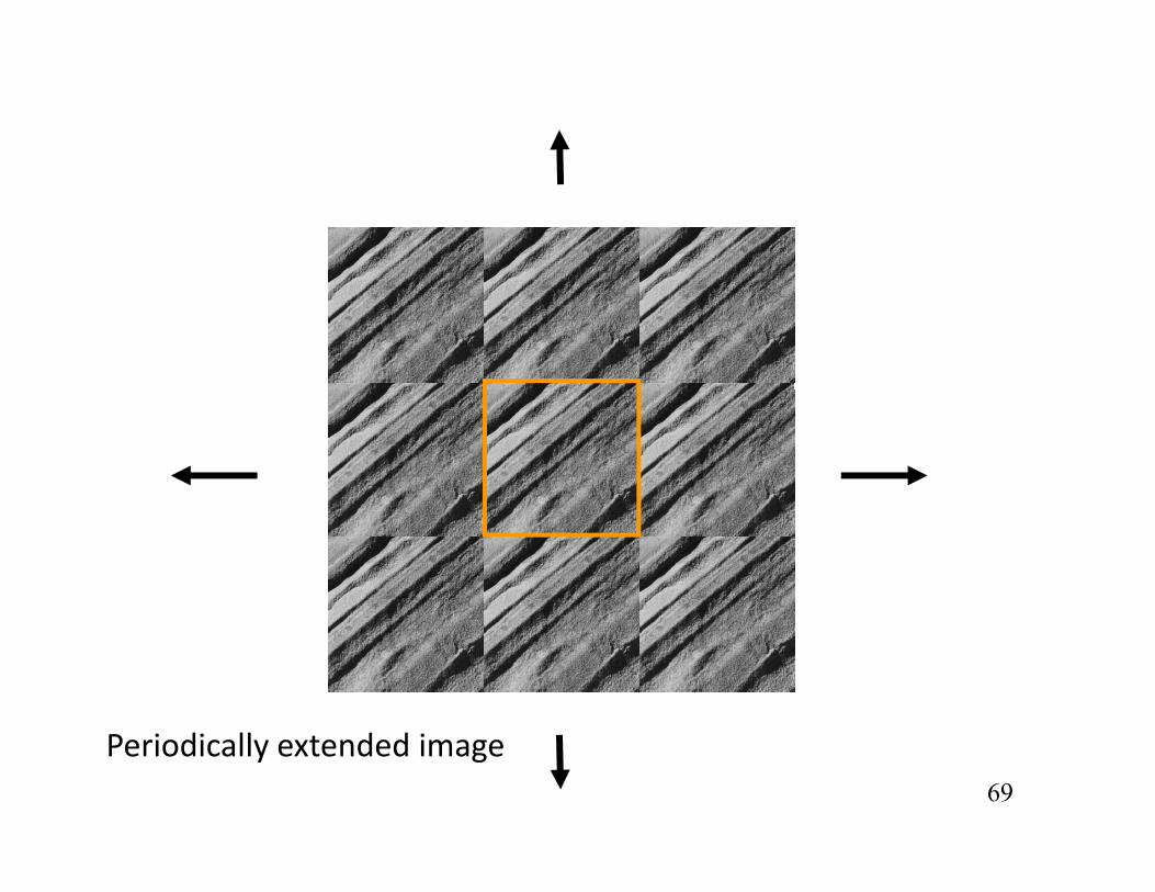
69

Periodically extended image

Displaying the Centered DFTDisplaying the Centered DFT• For interpretation, it’s usually desirable to display

h l i d i h ll f h lthe log-magnitude spectrum with all of the low frequencies together in the center (instead of at the corners – see page 4.63).corners see page 4.63).

• This can be accomplished using the frequency shift property of the DFT if we multiply the image I times an alternating image at the Nyquist rate:

+(-1) I( , )m n m n

• Taking the DFT of this modified image then produces the centered log-magnitude spectrum.

70• For images, this is how the DFT is normally viewed.

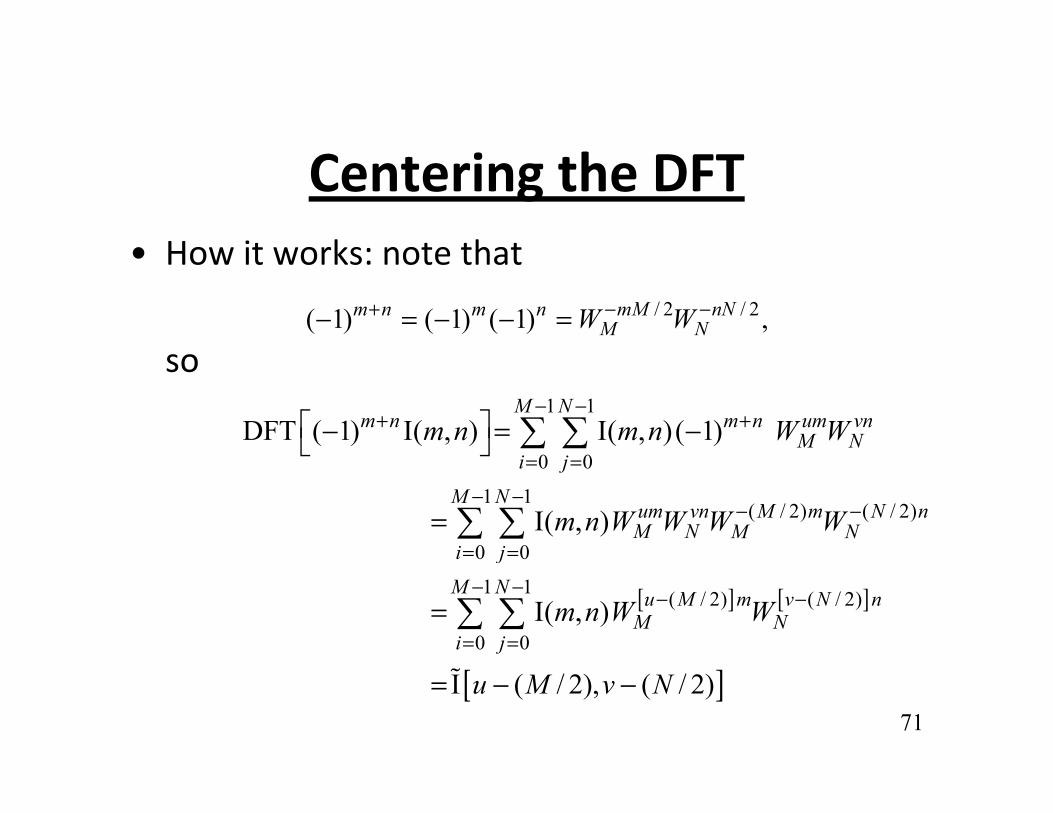
Centering the DFT• How it works: note that• How it works: note that

so

/ 2 / 2( 1) ( 1) ( 1) ,m n m n mM nNM NW W+ − −− = − − =

1 1

0 0DFT ( 1) I( , ) I( , )( 1)

M Nm n m n um vn

M Ni j

m n m n W W− −

+ + − = −

so

0 0

1 1( / 2) ( / 2)

0 0I( , )

i j

M Num vn M m N nM N M N

i jm n W W W W

= =

− −− −

= ==

[ ] [ ]1 1 ( / 2) ( / 2)

0 0I( , )

j

M N u M m v N nM N

i jm n W W

− − − −

= ==

[ ]I ( / 2), ( / 2)u M v N= − −71

72

Shifted (centered) DFT from periodic extension

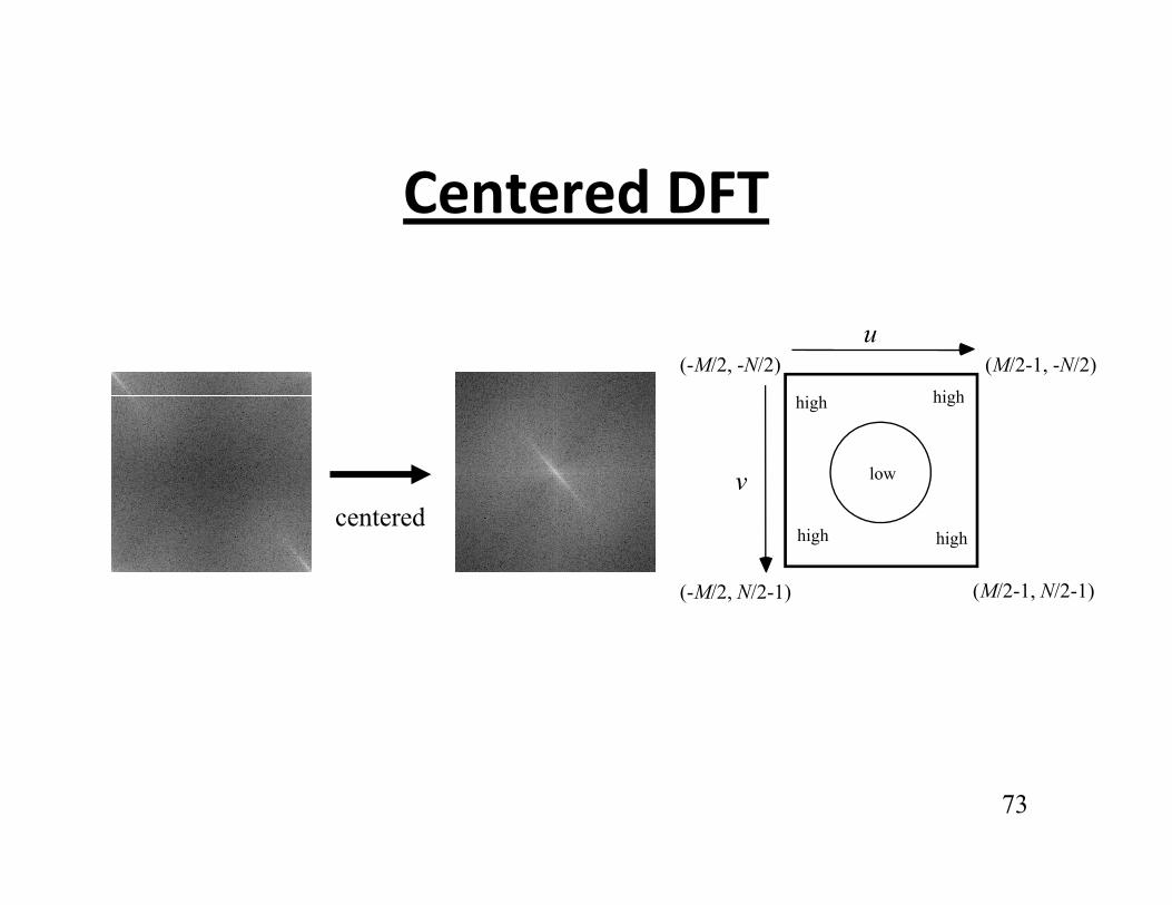
Centered DFT

u

high

(M/2-1, -N/2)(-M/2, -N/2)

dv

highhigh

low

centeredhighhigh

(M/2-1, N/2-1)(-M/2, N/2-1)

73

Understanding the Centered DFTUnderstanding the Centered DFT• Suppose the image I is 8×8.• This picture shows theThis picture shows the

frequencies u,v for every coefficient in the centered 2D DFT array.

• i j are the col/row indices for a Ci,j are the col/row indices for a C array. For Matlab, add 1.

• k is the offset from the base of the array in memory. For a 1D C array it is the index For a 1Darray, it is the index. For a 1D Matlab array, add 1.

• We think of the 2D frequency plane as being divided into fourplane as being divided into four quadrants:

Quadrant I: u≥0, v≥0Quadrant II: u<0, v≥0Quadrant III: u<0 v<0

74

Quadrant III: u<0, v<0Quadrant IV: u≥0, v<0

Understanding the Centered DFTUnderstanding the Centered DFT• Matlab provides builtin functions fft2 and ifft2 to compute

th 2D DFT ti 4 54 4 55the 2D DFT equations on pages 4.54-4.55.

• Matlab also provides a builtin function fftshift to center the DFT as shown on pages 4.70-4.73.p g– If the length of the DFT array is even, then applying fftshift a second

time will undo the shift.

– Matlab also provides a function ifftshift to undo the shift If theMatlab also provides a function ifftshift to undo the shift. If the length of the DFT array is odd, then you must use ifftshift.

• The Matlab FFT implementation calls an open source k d FFTW3package named FFTW3.

• If you use another language, you should also install FFTW3 and call it. There is a link to it on the course web site.

75

and call it. There is a link to it on the course web site.

Example• Let X1 be a cosine image with M=N=64 and u=v=8:

( ) ( 8 8 ) (8 8 )2 1 11 64 6464 2 2( , ) cos 8 + 8 W Wm n m nm n m nπ − − − − += = + X

• Note that MN=4096.• Following the pattern on page 4.74, the DC coefficient of the DFT array

( )1 64 6464 2 2( , )

(u=v=0) will be at (row,col) = (33,33) in a Matlab array or (32,32) in a C array.

• The real part of the DFT array will be equal to 4096/2 = 2048 at (u,v) = 1X(-8,-8) and (8,8).– This is (row,col) = (33-8, 33-8) = (25,25) and (33+8, 33+8) = (41,41) in

a Matlab array.

1

– Or (row,col) = (24,24) and (40,40) in a C array.

– Everywhere else, the real part of the DFT array will be zero.

• Because cosine is real and even the imaginary part of the DFT array is all

76

• Because cosine is real and even, the imaginary part of the DFT array is all zero.

Example• Let X2 be a sine image with M=N=64, u = -4, and v = 7:

( ) ( 4 + 7 ) (4 7 )22 64 6464 2 2( , ) sin 4 + 7 W Wj jm n m nm n m nπ − − − − −= − = + X

• We have again that MN=4096.• Because sine is pure imaginary and odd, the real part of the DFT array is

( )2 64 6464 2 2( , )

all zero.

• The imaginary part of the DFT array will be equal to -4096/2 = -2048 at (u,v) = (-4,7).

2X

– This is (row,col) = (33+7, 33-4) = (40,29) in a Matlab array.

– Or (row,col) = (39,28) in a C array.

• The imaginary part will be 4096/2 = 2048 at (u v) = (4 -7)• The imaginary part will be 4096/2 = 2048 at (u,v) = (4,-7).– This is (row,col) = (33-7, 33+4) = (26,37) in a Matlab array.

– Or (row,col) = (25,36) in a C array.

77

• Everywhere else, the imaginary part will be zero.

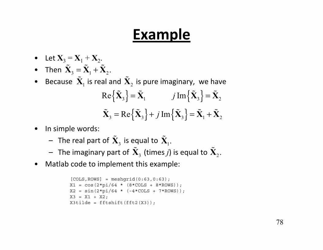
Example• Let X3 = X1 + X2.• Then

3 1 2.= +X X X • Because is real and is pure imaginary, we have2X1X

{ } { }3 1 3 2Re Imj= =X X X X

{ } { }

• In simple words:

– The real part of is equal to

{ } { }3 3 3 1 2Re Imj= + = +X X X X X

X X– The real part of is equal to

– The imaginary part of (times j) is equal to

• Matlab code to implement this example:

3X 1.X3X 2.X

[COLS,ROWS] = meshgrid(0:63,0:63);X1 = cos(2*pi/64 * (8*COLS + 8*ROWS));X2 = sin(2*pi/64 * (-4*COLS + 7*ROWS));X3 = X1 + X2;X3tilde = fftshift(fft2(X3));

78

X3tilde fftshift(fft2(X3));

>> imshow(255*((X1+1)/2),[0 255])>> imshow(255*((X2+1)/2),[0 255])>> imshow(255*((X3+2)/4),[0 255])

>>real(X3tilde(25,25))

ans =2.0480e+03

>>real(X3tilde(41,41))

ans =2.0480e+03

>>imag(X3tilde(26,37))

ans>> imshow(real(X3tilde),[0 2048])

ans =2048

>>imag(X3tilde(40,29))

ans =

>> imshow(imag(X3tilde),[-2048 2048])

-2048

79

Example in CExample in C

• On the course web site, there is a program “DoFFT.c” that implements this example in C.

• You can find it under the “code” link on the web site.

• It contains a function fft2d that calls FFTW3 to compute the 2D DFT andIt contains a function fft2d that calls FFTW3 to compute the 2D DFT and then centers it.

– Although only the forward transform is used in this example, fft2d can do both forward and inverse transforms.can do both forward and inverse transforms.

– There is a parameter “direction.” If direction=1, then it does the forward transform. If direction=-1, then it does the inverse transform.transform.

• The comment block at the top of the program explains how to compile it and link it to the FFTW3 library.

• You need to install FFTW3 before you compile the program

80

• You need to install FFTW3 before you compile the program.

Complex Exponential Matrix

• We define a special matrix of complex numbers:

1 1 1 1 1 1 2 3 -1

2 4 6 2( -1)

1 1 1 1 111

NN N N N

N

W W W WW W W W

3 6 9 3( -1)

11

N N N NNN

N N N N

W W W WW W W W

=

W

• Note that it is a symmetric matrix

2-1 2( -1) 3( -1) ( -1)1 N N N NN N N NW W W W

81

• Note that it is a symmetric matrix

Inverse Matrix

1 1 1 1 1

-1 *1 1=N NN N=W W

-1 -2 -3 1-

-2 -4 -6 -2( -1)

-3 -6 -9 -3( -1)

111

NN N N N

NN N N N

N

W W W WW W W WW W W W

N NN N

2

( )

1- -2( -1) -3( -1) -( -1)

1

1

N N N N

N N N NN N N N

W W W W

W W W W

N N N N

82

Matrix-Product Form of DFT

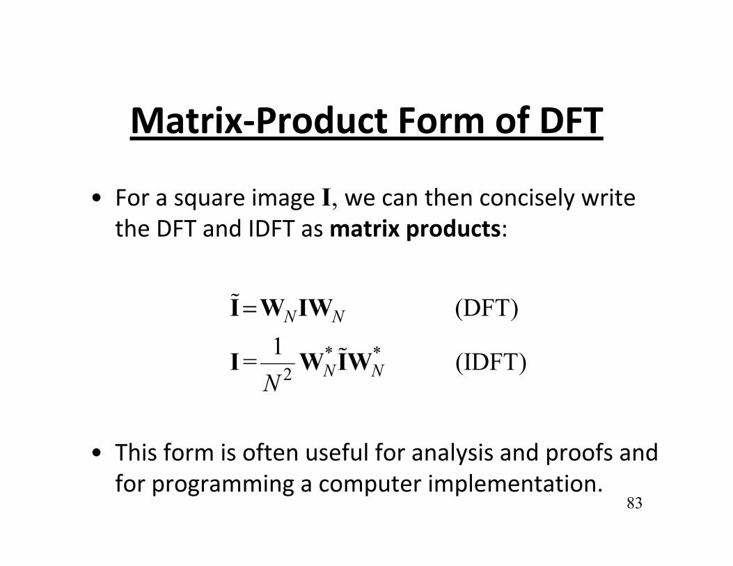
• For a square image I, we can then concisely write the DFT and IDFT as matrix products:

(DFT)N N=I W IW

* *2

( )1= (IDFT)

N N

N NNI W IW

• This form is often useful for analysis and proofs and

N

83

y pfor programming a computer implementation.

Computation of the DFTComputation of the DFT

• Fast DFT/IDFT algorithms are collectively referred to as the Fast Fourier Transform(FFT).

• Matlab provides routines fft2, ifft2, and fftshift (for centering).fftshift (for centering).

• For C, C++, and other languages, the FFTW package is strongly recommendedpackage is strongly recommended.

• The speedup is the same as in 1D: from (M2N2) to [MNlog(MN)]

84

(M2N2) to [MNlog(MN)].

Interpreting Spatial FrequenciesInterpreting Spatial Frequenciesin the Image

• It’s easy to lose track of the meaning of the DFT and the notion of frequency content in q yall the math.

• By examining the DFT or spectrum of an image (especially its magnitude) we canimage (especially its magnitude), we can often deduce much about the image.

85

Qualitative Properties of the DFT

• We may regard the DFT magnitude as an image of frequency content.

h h d " "• Bright regions in the DFT magnitude "image" correspond to frequencies having large magnitudes in the actual image.magnitudes in the actual image.

• It is intuitive to think of image frequency content in terms of granularity (distribution of radial frequencies) and orientation (distribution of frequency vector directions).

86

Image Granularity

• DFT coefficients near the origin correspond to

Image Granularity

g plarge, smooth structure in the image - often background.

• Since most images are non-negative, the DFT usually shows a strong peak at (u, v) = (0, 0).

• Low frequency = long wavelength = large-scale structure in the image.

• High frequency = short wavelength = small-scale structure in the image.

87

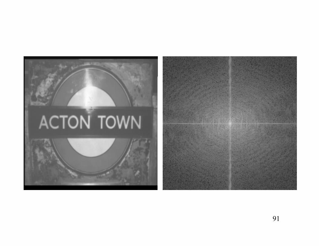
Image DirectionalityImage Directionality• Large DFT coefficients along certain orientations

correspond to directional structure in the image.

• When there are strong, oriented structures in the DFT, strongly directional structures will be visible in the image.

bl h d l d• Visible structure in the centered log-magnitude spectrum is orthogonal to the structure in the imageimage.

• This is because the direction of the frequency vector [u v]T is normal to the wavefronts in the

88

vector [u v] is normal to the wavefronts in the image (see page 4.40).

89

90

91

92

93

Granularity Selective Masking

• Define zero-one masks (black = 1)

l f k id f k hi h f k

• Masking (multiplying) a DFT with these will produce IDFT images retaining only low middle

low-frequency mask mid-frequency mask high-frequency mask

produce IDFT images retaining only low, middle, or high radial frequencies.

94

Granularity Selective Masking ( h )(white = 1)

95

Orientation Selective Masking

• Define oriented, angular zero-one masks:

• Multiplying these times the DFT and inverting will retainMultiplying these times the DFT and inverting will retain only the selected orientations.

96

Orientation Selective Masking ( h )(white = 1)

97

Chirp ImageChirp Image

98

Granularity Selective Masking ( h )(white = 1)

99

Orientation Selective Masking ( h )(white = 1)

100

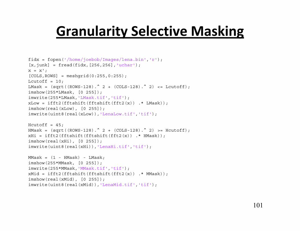
Granularity Selective Masking

fidx = fopen('/home/joebob/Images/lena.bin','r');[x,junk] = fread(fidx,[256,256],'uchar');x = x';;[COLS,ROWS] = meshgrid(0:255,0:255);Lcutoff = 10;LMask = (sqrt((ROWS-128).^ 2 + (COLS-128).^ 2) <= Lcutoff);imshow(255*LMask, [0 255]);imwrite(255*LMask,'LMask.tif','tif');xLow = ifft2(fftshift(fftshift(fft2(x)) .* LMask));imshow(real(xLow), [0 255]);imwrite(uint8(real(xLow)),'LenaLow.tif','tif');

Hcutoff = 45;HMask = (sqrt((ROWS 128) ^ 2 + (COLS 128) ^ 2) >= Hcutoff);HMask = (sqrt((ROWS-128). 2 + (COLS-128). 2) >= Hcutoff);xHi = ifft2(fftshift(fftshift(fft2(x)) .* HMask));imshow(real(xHi), [0 255]);imwrite(uint8(real(xHi)),'LenaHi.tif','tif');

MMask = (1 - HMask) - LMask;;imshow(255*MMask, [0 255]);imwrite(255*MMask,'MMask.tif','tif');xMid = ifft2(fftshift(fftshift(fft2(x)) .* MMask));imshow(real(xMid), [0 255]);imwrite(uint8(real(xMid)),'LenaMid.tif','tif');

101

Orientation Selective Masking

fidx = fopen('/home/joebob/Images/lena.bin','r');[x,junk] = fread(fidx,[256,256],'uchar');x = x'; ;[COLS,ROWS] = meshgrid(0:255,0:255);

Cp = 3*pi/4; % center angle (plus)Cm = Cp+pi; % center angle (opposite)W = pi/6; % anglular half-bandwidth U = COLS-128;V = ROWS-128;Theta = atan2(V,U);Mask = ((Theta >= Cp-W) .* (Theta <= Cp+W)) + ...

((Theta+2*pi >= Cp-W) .* (Theta+2*pi <= Cp+W)) + ...((Theta 2*pi >= Cp W) * (Theta 2*pi <= Cp+W)) +((Theta-2*pi >= Cp-W) .* (Theta-2*pi <= Cp+W)) + ...((Theta >= Cm-W) .* (Theta <= Cm+W)) + ...((Theta+2*pi >= Cm-W) .* (Theta+2*pi <= Cm+W)) + ...((Theta-2*pi >= Cm-W) .* (Theta-2*pi <= Cm+W));

imshow(255*Mask, [0 255]);imwrite(255*Mask,'Mask.tif','tif');, , ;y = ifft2(fftshift(fftshift(fft2(x)) .* Mask));%imshow(real(y), [0 255]);title('Orientation Masked Image');imwrite(uint8(real(y)),'y.tif','tif');

102

103

104

DISCRETE-SPACE FOURIER ( )TRANSFORM (DSFT)

• We have been looking at the 2D DFT. It’s the 2D version of the 1D DFTWe have been looking at the 2D DFT. It s the 2D version of the 1D DFT on page 4.22.

• In 1D, we usually use n for the time variable (or index) and k for the frequency variable (which you can think of as indexing the basis signals).frequency variable (which you can think of as indexing the basis signals).

• In a general ND formulation, you could use n = (n1 n2 … nN) for the “time” index and k = (k1 k2 … kN) for the frequency index.

• For the 2D case we used (m n) for the space index and (u v) for the• For the 2D case, we used (m,n) for the space index and (u,v) for the frequency index. We did this to minimize the use of subscripts. This is a widely used convention.

• Now we are going to look at the 2D version of the 1D DTFT on page 4 13• Now we are going to look at the 2D version of the 1D DTFT on page 4.13. It is called the 2D Discrete-Space Fourier Transform (DSFT).

• For the 2D DSFT, we will use (m,n) for the space variables and (U,V) for the frequency variables

105

the frequency variables.

THE DISCRETE-SPACE FOURIER ( )TRANSFORM (DSFT)

• Let the image I be defined on all of 2.• The 2D Discrete-Space Fourier Transform is given by:

( )2I ( ) I( ) (DSFT)j Um VnD U V m n e π∞ ∞ − += I ( , ) I( , ) (DSFT)D

m nU V m n e

=−∞ =−∞

( )1 12 21 12 2

2- -

I( , ) I ( , ) (IDSFT)j Um VnDm n U V e dU dVπ +=

106

Discrete-Space Fourier TransformDiscrete Space Fourier Transform• The units of U and V are cycles per pixel.

– We could alternatively use units of radians per pixel. The limits of integration in the IDSFT would then be -p to p and a factor of 1/(2p)2would then be p to p and a factor of 1/(2p)would be required on the IDSFT.

• The DSFT is periodic with period ONE along each axis.

• The DSFT is continuous in spatial frequency.• In most practical cases, the image I has a finite size.• For (m,n) outside the range 0 < m < M-1,

0 < n < N 1 we set I(m n) 0 for the DSFT107

0 < n < N-1, we set I(m,n) = 0 for the DSFT.

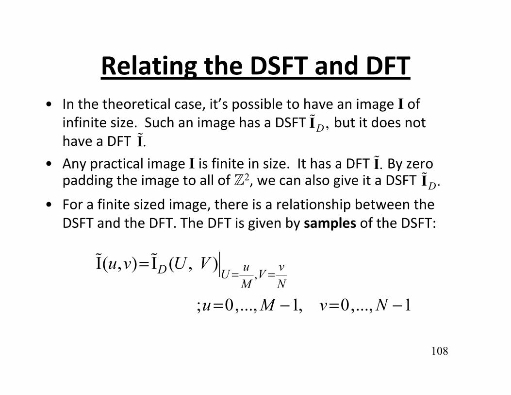
Relating the DSFT and DFTRelating the DSFT and DFT• In the theoretical case, it’s possible to have an image I of

infinite size Such an image has a DSFT but it does notIinfinite size. Such an image has a DSFT but it does not have a DFT

• Any practical image I is finite in size. It has a DFT By zero

,DI.I

.Ipadding the image to all of 2, we can also give it a DSFT

• For a finite sized image, there is a relationship between the DSFT and the DFT The DFT is given by samples of the DSFT:

.DI

DSFT and the DFT. The DFT is given by samples of the DSFT:

I( , ) I ( , ) u vD U Vu v U V=

,( ) ( )

; 0,..., 1, 0,..., 1

D U VM N

u M v N

= =

= − = −

108

DSFT

• It is more usual to introduce the DSFT first, followed by the DFT.y

• However, our emphasis is on algorithmsand applications which generally use theand applications, which generally use the DFT.

• We will find the DSFT to be a valuable• We will find the DSFT to be a valuable analytic tool.

109

SamplingSampling• We will now study the relationships between

th DFT/DSFT d th ti 2D F ithe DFT/DSFT and the continuous 2D Fourier transform of the original, unsampled optical image that exists inside the camera.image that exists inside the camera.

• The digital image I is a sampled version f h i i l i i iof the continuous optical intensity image

that is focused through the lens system to become incident upon a sensor

CI ( , )x ysystem to become incident upon a sensor located on the camera focal plane.

110

Notation and Units

• For the nD continuous Fourier transform on page 4.25, we used a vector x for the spatial variable and a vector u for the frequencyvector x for the spatial variable and a vector u for the frequency variable.

• For 2D continuous optical images, we will use x = (x, y) to avoid subscripts Thus we will write I (x y)subscripts. Thus, we will write IC(x, y).

• The spatial coordinates (x, y) can be expressed in mm, inches, or any other appropriate unit of length.

• Often it is convenient to express them in units given by the• Often, it is convenient to express them in units given by the horizontal and vertical detector spacings on the focal plane, i.e., in units that are given by the physical size of a pixel in the camera.

• Again to avoid subscripts we will write the 2D continuous Fourier• Again to avoid subscripts, we will write the 2D continuous Fourier transform frequency variable as u = (Ω,Λ), where Ω = horizontal frequency and Λ = vertical frequency.

111

Continuous Fourier Transform

• The continuous image has a Continuous Fourier Transform (CFT) where (x,y) are

CI ( , )x y

CI ( , )Ω Λspace coordinates and (Ω, Λ) are Hertzian spatial frequencies:

( )2C C- -

I ( , ) I ( , ) (CFT)j x yx y e dxdyπ∞ ∞ − Ω +Λ∞ ∞

Ω Λ =

( )2C C- -

I ( , ) I ( , ) (ICFT)j x yx y e d dπ∞ ∞ Ω +Λ∞ ∞

= Ω Λ Ω Λ

112

Continuous Fourier TransformContinuous Fourier Transform

• The CFT is not periodic in general.p g

• The horizontal frequency Ω and vertical• The horizontal frequency Ω and vertical frequency Λ are continuous and expressed in cycles per unit of length i e per unit ofin cycles per unit of length, i.e. per unit of (x,y).

h f l h b f d• The unit of length must be specified. For convenience, we will usually assume it is h h h / d h f l h d

113the height/width of a pixel on the detector.

Relating the CFT and DSFT/DFT

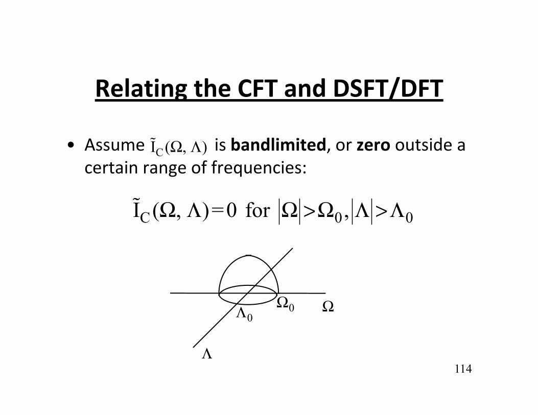
• Assume is bandlimited, or zero outside a certain range of frequencies:

CI ( , )Ω Λ

C 0 0I ( , )=0 for ,Ω Λ Ω >Ω Λ >Λ

0Ω0Λ Ω

114Λ

On Bandlimitedness• Any real-world image is approximately

bandlimited: its CFT becomes vanishingly smallbandlimited: its CFT becomes vanishingly small for large Ω, Λ.

• If it were not so the image would contain infinite• If it were not so the image would contain infinite energy since (Parseval)

22C C- - - -

I ( , ) I ( , )x y dxdy d d∞ ∞ ∞ ∞∞ ∞ ∞ ∞

= Ω Λ Ω Λ

• Ex: a Gaussian image has a Gaussian CFT which is not bandlimited. But the integrals converge b h CFT i h Ω Λ

115

because the CFT vanishes as Ω,Λ ∞.

Image Sampling• The detector creates I(m n) by sampling the optical• The detector creates I(m,n) by sampling the optical

image with spacings X, Y in the x- & y-directions:

I( ) I ( ) ; 0 1 0 1m n mX nY m M n N= = =

• The DSFT and CFT are related by:

CI( , ) I ( , ) ; 0 ,..., 1, 0 ,..., 1m n mX nY m M n N= = − = −

• The DSFT and CFT are related by:

C1I ( , ) I ,

XY X YDp qU V

∞ ∞ = Ω − Λ −

( )

( ) ( )

X Y- - ( , ) ,XY X Y

1 1 1I

U Vp q

U p V q

= ∞ = ∞ Ω Λ =

∞ ∞

= − −

116

( ) ( )C- -

I , XY X Yp q

U p V q= ∞ = ∞

=

Relating DFT to CFT

• We have:

I( , ) I ( , ) u vDu v U V= ,

C

( , ) ( , )

1 1 1I , XY X Y

u vD U VM N

u vp qM N

= =

∞ ∞ = − −

• A sum of shifted versions of the CFT. It is periodic in

- -XY X Yp q M N= ∞ = ∞

A sum of shifted versions of the CFT. It is periodic in the u- and v-directions with periods 1/X and 1/Y, respectively.

117

u

v

118

Unit-Period CaseUnit Period Case• We can always set X = Y = 1.

• This simply says that we measure length and area in units that are given by the physical size of a pixel on the detector array (usually on the order of

i )microns).

• Then

CI( , ) I , u vu v p qM N

∞ ∞ = − −

119

- -p q M N= ∞ = ∞

Sampling Theorem1 1

• If or the replicas of the CFT

will overlap (sum up) distorting them This is

01

2XΩ > 0

1 ,2Y

Λ >

will overlap (sum up), distorting them. This is called aliasing.

• The digital image can be severely distorted.g g y• To avoid aliasing, the sampling frequencies 1/X

and 1/Y must be at least twice the highest frequencies Ω0 and Λ0 in the continuous image.

120

Comments on Sampling

• This is a mathematical reason why images must be sampled sufficiently densely. If p y yviolated, image distortion can be visually severe.

• If the Sampling Theorem is satisfied then• If the Sampling Theorem is satisfied, then the DFT is periodic (sampled) replicas of the CFT

121

CFT.

Aliased Chirp ImageAliased Chirp Image• A chirp image

[ ] ( )2 2CI ( , ) cos ( , ) cos x y A x y A ax byϕ= = +

has instantaneous spatial frequencies

( ) ( )( ) ( ) ( ) 2 2bΩ Λ

which increase linearly away from the origin.

( ) ( )inst inst( , ) ( , ), ( , ) 2 , 2x yx y x y ax byϕ ϕΩ Λ = =

y y g

• For such an image, the origin (x,y) = (0,0) is usually taken at the center of the image.

122

g

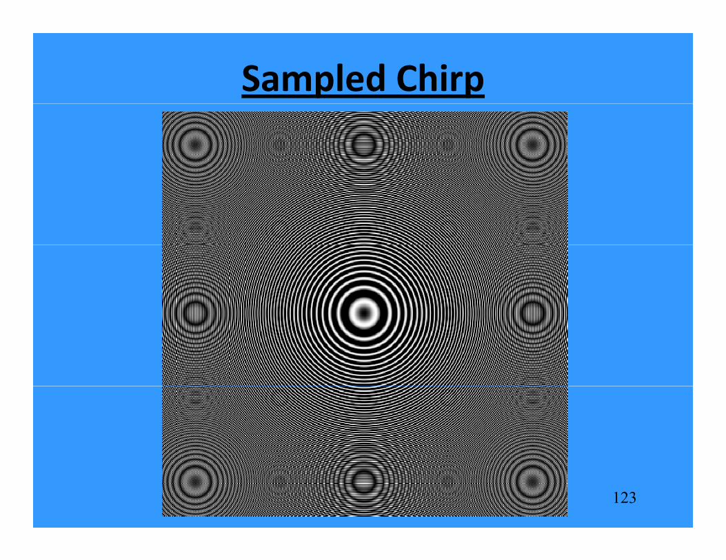
Sampled Chirp

123

Aliased ImageAliased Image

S d D I C t d DFT Sh i Ali i124

Sand Dune Image Centered DFT Showing Aliasing

IMPORTANT 2-D FUNCTIONSIMPORTANT 2 D FUNCTIONSAND THEIR DFTS

• It is worthwhile to examine the DFTs of some specific images. This is usually hard p g yto do explicitly by hand for the DFT/DSFT.

• So we'll give some simple onesSo we ll give some simple ones.

• Then state some others as CFT transform pairspairs.

125

Constant Image

• Let I(m,n) = c for 0 ≤ m ≤ M-1, 0 ≤ n ≤ N-1• Then

whereI( , ) ( , )u v c MN u vδ=

1 ; 0( , )

0 ; elseu v

u vδ= == =

unit impulse

0 ; else

126

2-D Unit Pulse Image

• Let I(m,n) = cδ(m,n)• Then

-1 -1I( , ) ( , )

M Num vnM Nu v c m n W Wδ=

0 00 0

m n

N McW W c= =

= = (constant DFT)

127

Cosine Wave Image

• Let- -I( , ) cos 2

2bm cn bm cnM N M N

b cM N

dm n d m n W W W Wπ = + = + • Then

2M N

1 1 -1 -1- -

0 0-1 -1

( ) ( ) ( ) ( )

I( , ) 2

N Mbm cn bm cn um vnM N M N M N

m nN M

b b

du v W W W W W W

d= =

+ +

= +

[ ]

( ) ( ) ( - ) ( - )

0 0

2

( , ) ( , )

u b m v c n u b m v c nM N M N

m n

d W W W W

d MN u b v c u b v cδ δ

+ +

= =

= +

= − − + + +

128

[ ] ( , ) ( , ) 2

MN u b v c u b v cδ δ+ + +

Sine Wave ImageSine Wave Image

• Likewise if• Likewise, if

I( , ) sin 2 b cM N

m n d m nπ = +

then

M N

[ ]I( , ) ( , ) ( , ) 2du v j MN u b v c u b v cδ δ = + + − − −

• The Fourier representations of pure sinusoids are d i l f i

129

concentrated single frequencies

DFT AS A SAMPLED CFTDFT AS A SAMPLED CFT

• Now some CFT pairs that are either difficult pto express or are too lengthy to do by hand as DFT (or even as DSFT) pairs.( ) p

• If sampled adequately, then

the DSFT is given by appropriately scaled– the DSFT is given by appropriately scaled periodic repetitions of the CFT.

h DFT i i b l f h DSFT– the DFT is given by samples of the DSFT.

130

Rectangle FunctionRectangle Function

• Let A B

• Then

C

A B; ,I ( , ) = rect rect = 2 2

A B 0 ; else

c x yx yx y c ≤ ≤ ⋅ ⋅

• Then ;

( ) ( )CI ( , ) = A B sinc A sinc BcΩ Λ ⋅ ⋅ ⋅ Ω ⋅ Λ

where

1( ) ( )11 ; sin

rect = sinc(x) = 20 ; else

x xx

xπ

π

≤

and

131

;

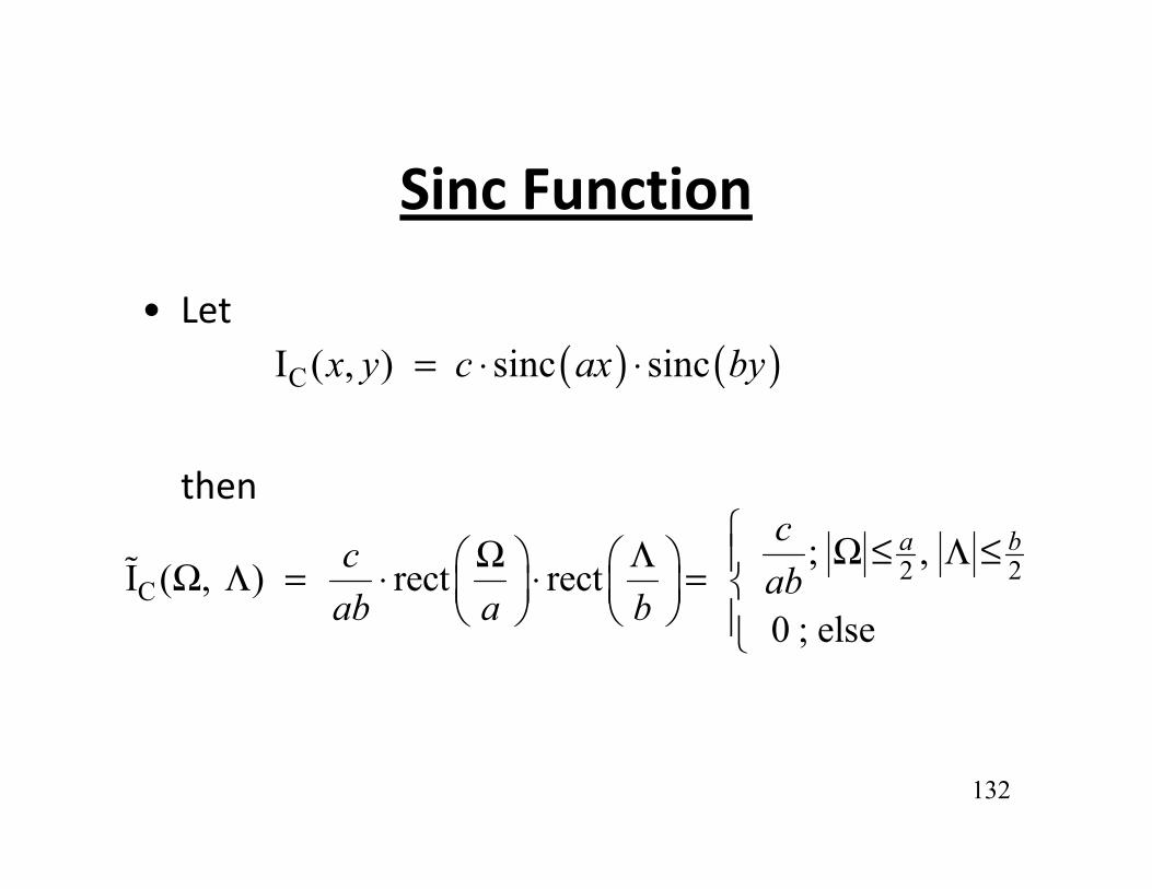
Sinc Function

• Let( ) ( )CI ( , ) sinc sincx y c ax by= ⋅ ⋅

then

2 2C

; ,I ( , ) rect rect

a bcc

abab a b

Ω ≤ Λ ≤Ω Λ Ω Λ = ⋅ ⋅ =

0 ; else ab a b

132

Gaussian FunctionGaussian Function

• Let ( )2 2x y − +

then

( )C 2I ( , ) exp

x yx y

σ

+ =

( ) ( )2 2 2 2 2CI , expπσ π σ Ω Λ = − Ω + Λ

• The Fourier transform of a Gaussian is also Gaussian – an unusual property.p p y

• Note: since is not bandlimited, the digital image will be aliased.

( )CI , Ω Λ

133

Comments

• We now have a basic understanding of frequency-domain concepts in 2D.q y p

• Let’s put them to use in linear filtering applications onward to Module 5applications… onward to Module 5.

134