MCVisionWP1A_2003

Implementing a Machine Vision Systems

A Step-by Step Guide to Implementation

Jason Reid Neo Vista System Integrators

Table of Contents Introduction Page 3 The Launch Page 4 Cost Justification Page 5 Specification Page 6 The Base Design Page 8 Proving Feasibility Page 24 Specification Outline Page 29 Pre-Launch Checklist Page 32 Initial Design Worksheet Page 33

3

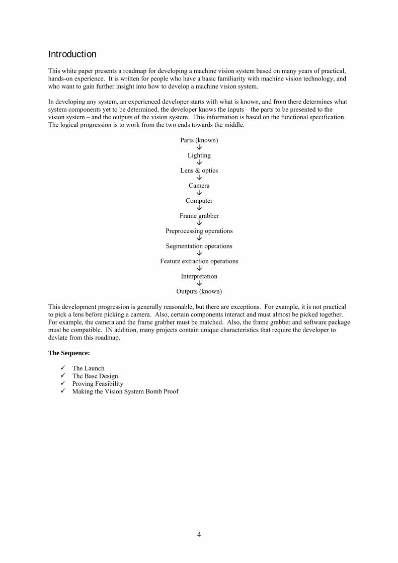
Introduction This white paper presents a roadmap for developing a machine vision system based on many years of practical, hands-on experience. It is written for people who have a basic familiarity with machine vision technology, and who want to gain further insight into how to develop a machine vision system. In developing any system, an experienced developer starts with what is known, and from there determines what system components yet to be determined, the developer knows the inputs – the parts to be presented to the vision system – and the outputs of the vision system. This information is based on the functional specification. The logical progression is to work from the two ends towards the middle.

Parts (known)

Lighting

Lens & optics

Camera

Computer

Frame grabber

Preprocessing operations

Segmentation operations

Feature extraction operations

Interpretation

Outputs (known) This development progression is generally reasonable, but there are exceptions. For example, it is not practical to pick a lens before picking a camera. Also, certain components interact and must almost be picked together. For example, the camera and the frame grabber must be matched. Also, the frame grabber and software package must be compatible. IN addition, many projects contain unique characteristics that require the developer to deviate from this roadmap. The Sequence:

The Launch The Base Design Proving Feasibility Making the Vision System Bomb Proof

4

The Launch Before building a machine vision system, there are a number of factors that are necessary or have proven very valuable. These are:

The champion Management support Team with necessary skills Specification Acceptance test procedure

Champion The champion is a person who is personally committed to the success of the project. He may or may not be a major contributor, but is willing and able to put forth whatever effort is necessary to see the project succeed. The champion does not have to be in management, but people in the enterprise must recognise the person as a leader. And, of course, they must be available.

Management Support Key managers are decision makers who can provide resources to the project. Unless these managers are sufficiently interested, the necessary resources will not become available. The managers are not necessarily needed on a day-to-day basis, but they keep abreast of progress by attending meetings and asking questions about periodic reports. To get management’s attention and support, the project must:

Address a major goal of the enterprise Meet investment criteria Overcome management’s caution toward risk

For best results, the project should have a written proposal. In some larger, well established enterprises, there is a well defined procedure for obtaining project approval that includes a formal proposal. In some smaller enterprises, projects are handled more informally, but the value of a written proposal that lays out the costs, benefits, and schedule is well worth the time and effort.

5

Cost Justification The cost justification looks at a cash flow over time – expenses as well as benefits. In some enterprises, the result is an ROI calculation; in others it is a break-even analysis. Costs

Initial costs Equipment purchase System development and integration Installation Training Project management

Operating costs

Utilities Maintenance Retaining Upgrades

Machine vision systems range I cost form $1,500 to $7,000,000 not including installation. It is impractical and misleading to suggest any specific budgetary amount. Likewise, other costs will vary considerably depending on the specific requirements and circumstances. There are exemplary cases where machine vision systems have paid for themselves in the first month of operation. There are other cases of successful machine vision systems which took from three to seven years to reach breakeven. The investment criteria depend on the enterprise and vary depending on economic conditions. Benefits Machine vision offers many potential benefits. Some, like labour savings, are easy to quantify. Others, like improved customer confidence, are much more difficult to quantify. Most machine visions systems are justified on the basis of one or more of the following:

Labour savings Scrap reduction Quality improvement Technical necessity

Only benefits which can be quantified are usable in cost justification. Other benefits, and there may be several for a typical machine vision application, should be noted in the project proposal. Overcoming Caution Towards Risk The best tools a developer has at his disposal for dispelling management’s caution toward risk are a good project proposal that shows thought and planning, and case studies that illustrate how machine vision succeeds. Successful examples from the manager’s operation are the most persuasive. Otherwise, case studies from the literature can be very helpful.

6

The Team No one person has all the skills necessary to address the typical machine vision requirements. These skills are typically:

Project management Process engineering Part handling Equipment packaging Optics Electronics Software Training Maintenance

The team may consist of people from other organisations that will be using the vision system (e.g., process engineering), the people or person who will be doing the actual vision system integration, suppliers of hardware and software, and consultants. Many skills are needed only for a brief time during the project. Specification The functional specification is often a neglected part of the project. No wonder. To people close to the requirement the specification often seems almost obvious. A good specification takes time and effort to prepare. Also, some people may feel a specificaiton is too rigid, and does not provide the flexibility needed to effectively manage the project. Finally, people who have not been involved with machine vision do not know what needs to be specified, and rely on the person receiving the specification to ask for missing information. Each of these reasons for not producing or requiring a good specification is fallacious. The specification need not be rigid. It can be a living document that changes as questions arise and are addressed. The ideal specification gives the reader a brief background on the requirement including how the operation is presently performed, if at all, and what benefits the machine vision system will provide. It provides both minimum requirements as well as desirable enhancements. One fault with some specifications is that they ask for too many options. This creates a mix-and-match nightmare for anyone proposing the system. For example, rather than having a proposal address requirements for 50 parts/minute and for 75 parts/minute, the specification could state that 50 parts/minute is the minimum requirement, but that increased speeds up to 75 parts/minute will receive favourable consideration. Thus, the developer in writing the proposal can specify the best performance their equipment will offer. A details outline for a specification is offered in the appendix at the end of this paper. In general, the specification should address these areas:

General description – includes how the operation is currently performed, if at all, and what benefits are expected from the machine vision system.

Description of objects – their size, colour, normal and unusual variation, etc, as well as the number of different parts.

Performance requirements – speed, accuracy, reliability, etc. Part presentation – how the parts will be brought into the camera’s view and how many parts will be in

view at one time. Optical – field-of-view, standoff distances, etc. Physical and mechanical requirements – size limits, mounting requirements, enclosures needed. Utilities available – electrical power, compressed air, cooling water, etc. Environment – ambient light, temperature, humidity, dirt, dust, mist, plant cleaning procedures. Equipment Interface (I/O) – networking and closely coupled devices. Operator interface – screens, controls, operator privileges. Support requirements – training, maintenance, and upgrades. Future modifications – upgrades or changes that are anticipated or likely.

7

Acceptance Test Procedure Typically, an acceptance test is performed when a system is ready for installation, and a buy-off test is performed after installation as the system is commissioned for operation. Ideally, these two tests would be very similar. However, there are sometimes aspects of the system that cannot be tested before installation (e.g., sustained production speed), and portions of the test do not necessarily need to be repeated after installation (e.g., sequence of user screens). Although it is not essential that the acceptance test be available at the project launch, it often provides the developer with invaluable insights into how to design the system. Thinking through the test procedure can identify functions that will facilitate the test. For example, if a vision system is to verify some attribute, say a hold in a part, it usually makes some sort of measurement, and declares the hold present if the measurement satisfies some criteria. The testing required to verify the system’s reliability in detecting the hole is much greater if it is based on just the attribute reporting. But if the measurement of the hold is made available, a simple statistical analysis on the measurement information can give a sound indication of reliability with a much shorter test. The acceptance test should address the following general areas:

Operator interface – are all controls and screens present and functional? Basic operation – can expected procedures be performed? Accuracy and repeatability – does the vision system provide quality results? Throughput – does the vision system meet speed requirements? Sensitivity – will minor change sin the environment or system settings (e.g., light level) cause major

performance problems? Maintainability – are basic maintenance procedures (e.g., replacing a lamp) and calibration procedures

easy to perform? Availability – what percentage of the time is the system available for use?

The acceptance test will require a comprehensive set of samples. However, the same set of samples will be invaluable during the entire development process. A good set should span the entire range of objects that the vision system will need to image, from the largest to the smallest and from the best to the worst. Additionally, the sample sin the set should be calibrated (e.g., 5.84mm diameter or this is a type 3 defect). Collecting and calibrating a comprehensive set of samples is a significant undertaking. While it is not essential that the sample set be complete at the time the project is launched, it is essential that the sample set be complete before system development proceeds too far. The sample set is more important than the specification. In developing a machine vision system, there is no substitute for having parts to put under a camera. The test of a good sample set is whether or not all parties are comfortable developing and accepting the vision system based solely on the set of samples provided for development.

8

The Base Design Subsequent to the launch of a machine vision project, there are several initial design steps that need to be performed. These steps all contribute toward obtaining an image. The steps are:

Choose the type of camera Choose the camera view Calculate the field-of-view Evaluate resolution Ballpark speed Select hardware processing option Select the camera Select the lens Select the lighting technique Select the frame grabber Plan the image processing Choose the software package

The order shown is not in strict sequence from input (parts) to output (image). This change in order is because in some cases (e.g., camera and lens), it is far easier to select the first after the second has been determined. Also, some steps are completed very quickly compared to others (e.g., resolution evaluation is usually more straightforward than lighting technique selection), and it is more efficient to do the easy things first. Choose the Type if Camera In machine vision, there are 1-dimensional cameras (line-scan cameras), 2-dimensional cameras (area cameras), and a host of 3-dimensional imaging techniques. This white paper will address the use of line-scan (1-dimensional) and area (2-dimensional) cameras only. The range of 3-dimensional techniques is too great to consider here. The majority of machine vision applications use area cameras, although some applications require the special requirements of a line-scan camera. Generally, choose to use area cameras unless the application imaging requirements has one of the following characteristics, in which case line-scan cameras should be chosen:

Making one-dimensional measurement in a fixed location Imaging a moving web (e.g., paper) Imaging mass conveyed parts Imaging the periphery of a cylinder where the cylinder can be rotated Very high resolution imaging of discrete parts where high-resolution cameras would be too expensive

and the part or camera can be moved Within the classes of line-scan and area cameras there are numerous additional choices (e.g., monochrome or color). In some cases, like the choice between monochrome and color, the choice might be obvious given the requirements. But in general, picking the specific camera features is left for later. Choose the Camera View To choose where the cameras will view the scene or part requires knowledge of several matters: where the features of interest are on the part; what features could confuse the vision system (if any) and where they are located on the part; the pose of the part (its location and orientation including variations); and other equipment that will restrict the camera's position (e.g., a robot arm). This information should all be available from the specification. There are some special cases that should be mentioned. One is when the parts being imaged are only partially constrained. That is, they are able to translate or rotate in several directions. If the parts cannot be constrained, it may take analysis to determine an array of views that can guarantee the desired features will be imaged. In addition, there is the challenge of determining which cameras are viewing the desired features during operation. In general, it is better to be able to constrain the part's pose to ensure the necessary features are imaged with a minimum number of cameras.

9

A second case is the situation where the camera must view through a mechanism such as a robot arm. This is especially complex when the mechanism can be moving during the imaging. Situations like these require coordination between the vision system and the mechanism's controller to ensure the camera will not be occluded while imaging the part. A third case worthy of note is where the camera will be mounted on a robot ann. This is done in those applications where it is desirable to change the camera's view to, say, adapt to different parts. It is also very useful where the image information must provide an offset for robot position as in precision assembly. Calculate the Field-of-View Knowing the type of camera and the camera's view provides sufficient information to calculate the field-of-view for each camera. The field-of-view in one direction can be found from: FOV = (Dp + Lv)(1 + Pa) where: FOV is the required field-of-view in one direction Dp is the maximum part size in the field-of-view direction Lv is the maximum variation in part location and orientation Pa is the allowance for camera pointing as a percentage or fraction The maximum part size (Dp) and the variation in part location and orientation (Lv) should be available from the application's specification. The parameter allowance for camera pointing (Pa) is an engineering judgment. It is obviously never desirable to have important features in the image touch the edge of the image. Also, it is relatively impractical to have a camera that must be aligned to within one pixel and to maintain that alignment in a manufacturing environment. The factor by which the field-of-view should be expanded depends to a great degree on the skill of the people who maintain the vision system. A value of 10% is a common choice. Example:

The part is rectangular, 3cm x 6cm maximum in size. It may be out of position (translation) by 0.5cm in any direction, but will not be rotated. Determine the minimum field-of-view.

From the requirements, Dp(horiz) is 6cm, and Dp(vert) is 3cm. We are assuming an area camera with a width greater than height, and chose the part dimensions to fit most comfortably in this rectangle. Lv is twice O.5cm or 1cm since the part can move in either direction by that much. For engineering purposes, Pa is set to 10%.

Calculating for field-of-view requirements:

FOV(horiz) = (6cm + 1cm)(l + 10%) = 7.7cm FOV(vert) = (3cm + lcm)(1 + 10%) = 4.4cm

Note that the required field-of-view has an aspect ratio of 7:4. The camera chosen will probably have a different aspect ratio (4:3 is typical for CCTV cameras); so, the final camera field-of-view will likely be larger in one direction than the calculated field-of-view.

Evaluate Resolution There are five types of resolution used in machine vision. They are:

Image resolution Spatial resolution Feature resolution Measurement resolution Pixel resolution

10

In general discourse, all are called "resolution". It is up to each individual to understand which resolution is being referenced. Image Resolution Image resolution is the number of rows and columns of pixels in the image. It is determined by the camera and its image sensor and by the frame grabber. For area cameras, typical image resolutions are 640x480 (expressed in columns and rows of pixels) and 1000x1000. Higher and lower image resolutions are available. For line-scan cameras, typical image resolutions are 256, 512, 1024, and 2048 (the number of rows is not expressed because it is always 1). For line-scan cameras, image resolutions can extend up to 8,000. The system developer when selecting the camera and frame grabber determines image resolution. If the camera and the frame grabber share a pixel clock, then there is a one-to-one correspondence between the pixels developed by the camera and those supplied by the frame grabber to the computer. When there is no shared pixel clock between the camera and frame grabber, such as when using a CCTV camera, then the pixels created by the frame grabber when it periodically digitizes the analog video will not be synchronized with the photo detectors in the camera's image sensor. Most practitioners of machine vision then use the lower of the two image resolutions, camera or frame grabber. However, in this situation there can be minor distortions along each raster line. Spatial Resolution Spatial resolution is the spacing between pixel centers when they are mapped onto the scene; it has the dimensions of physical length per pixel (e.g., 0.1 cm/pixel). It is determined by the image resolution and the size of the field-of view. Note that for a given image resolution, spatial resolution depends on the field-of-view or the magnification of the imaging lens. For example, a given camera and frame grabber might be set up to image a railroad boxcar with a spatial resolution of 2 inches/pixel. The same camera and frame grabber, and thus the same image resolution, might be mounted on a microscope to image an integrated circuit with a spatial resolution of 1 pm/pixel. The only difference in these two situations is the optical magnification. In the literature, spatial resolution is sometimes called pixel resolution. We reserve the term pixel resolution for a different purpose. Feature Resolution Feature resolution is the smallest feature reliably imaged by the system. It is a linear dimension (e.g., O.O5mm). Note that the definition uses the word "reliably". Thus while an artifact smaller than a pixel might sometimes appear in an image, its appearance would be unreliable. Because cameras and frame grabbers are sampled data devices (the pixel is a data sample), there is a principal called Shannon's Sampling Theorem that states it will take at least two pixels to represent an artifact in the image. Because practical technology does not usually reach theoretical limits, three to four pixels spanning the minimum size feature is a practical limit. The limit of three or four pixels spanning a feature assumes good contrast and low noise. If the image is low in contrast, or the image noise is high, then more pixels may need to span the feature for reliable detection. Also, this limit affects the detectability of a feature. While a feature that spans only three or four pixels may always appear in an image, it will not be measurable with any degree of accuracy. That is, a system that must discriminate between a feature that is four pixels wide and one that is three pixels wide will be very unreliable. Measurement Resolution Measurement resolution is the smallest change in an object's size or location that can be detected. It is a linear dimension (e.g., 0.05mm). While our raw data is in pixels, we have powerful data fitting techniques that fit image data to models (e.g., a straight line). From statistics, both theoretical and applied, we know that if we have N observations (measurements), each with an associated error ε, then the error of the average, εavg = ε½.

11

In the laboratory, measurement resolutions of better than 1/1000h of a pixel have been obtained. In practice, 1/10th pixel is considered achievable. The achievable measurement resolution depends on the sophistication of software algorithms to fit to pixel data, the error associated with the position of each pixel, and the number of pixels that can be combined to fit to the model. It also depends on how well the model matches the actual object. Measurement resolution is equivalent to the repeatability of a measurement. Most functional specifications will specify either a part's tolerance or the accuracy to which it must be measured. A system can have good repeatability (resolution) while being very inaccurate. Generally measurement errors can be classed into either random or systemic. Random errors are not predictable, and therefore not correctable. They degrade both accuracy and repeatability. Systemic errors are those errors which do not affect repeatability and can be characterized. Systemic errors can be corrected through calibration techniques. Traditionally, measurement requirements were specified with accuracy 10 times better than tolerance, and resolution 10 times better than accuracy. This means that the measurement resolution must be 100 times better than the part's tolerance As desirable as these ratios are, they are not cast in concrete. Part of the reason for their existence is to mitigate human error. With automated measuring tools, the human error has been eliminated. For automated systems, ratios of 4 or 5 are more commonly used, with a total ratio of around 20 (tolerance to resolution) being reasonable. Pixel Resolution Pixel resolution is the granularity of a pixel; that is the number of gray-levels or colors that are represented in a pixel. Pixel resolution is commonly called quantisation in the scientific literature. In other literature it is sometimes called gray-scale resolution. Pixel resolution is a function of the analog-to-digital converter located either on the frame grabber or in the camera. Monochrome machine vision systems most commonly use 8 bits per pixel, giving 256 gray levels. Monochrome images are digitized to 10 bits (1,024 gray levels) or 12 bits (4,096 gray levels) for scientific work. Color systems commonly use 8 bits for each of the three primary colors (red, green, and blue) for a total of 16,777,216 colors. Evaluating Resolution The application requirements give information from which to determine feature resolution required, measurement resolution required, or sometimes both. If the requirement is to detect some small feature, such as a defect, then the minimum size feature will determine feature resolution Rs = FOV/Ri Ri = FOV/Ri Rm = Rs Mp Rs = Rm Mp Rf = Rs Fp Rs = Rf Fp Where: Rs is the spatial resolution (may be either X or Y) FOV is the field-of-view dimension in either X or Y R Ri is the image resolution; number of pixels in a row (X dimension) or column (Y dimension) Rm is the desired measurement resolution in physical units (e.g. millimeters) MP is the vision system's measurement resolution capability in pixels or fraction of a pixel Rf is the feature resolution (smallest feature that must be reliably resolved) in physical units (e.g.,

millimeters) FP is the number of pixels that will span a feature of minimum size

12

Let's look at two examples. In both of these examples an area camera will be used, and the camera's field-of-view will be 4cm x 3cm. Example 1: The specification calls for detection of a hole in the part that is O.5mm diameter. This tells us the feature resolution (Rf) is O.5mm. As the developer we need to determine the minimum number of pixels that need to span this hole (Fp). Because we expect good contrast and reasonably low noise, we will set F equal to 4 pixels. Note that since the hole is round, these numbers are the same both horizontally and vertically. Knowing the feature resolution (Rf) and number of spanning pixels (Fp) we can compute the spatial resolution (Rs). Again, the calculated Rs will be the same horizontally and vertically. Rs = Rf / FP = O. 5mm / 4 pixels = 0.125mm/pixel From the spatial resolution (Rs) and the field-of-view (FOV), we can determine the image resolution.

Ri(horiz) = FOV (horiz) / Rs = 4cm / 0.125mm/pixel = 320 pixels Ri(vert) = FOV (vert) / Rs = 3cm / 0.125mm/pixe1= 240 pixels

So the minimum acceptable image resolution is 320 x 240 pixels. Example 2: A part having a tolerance of ±O.O5mm must be measured. Also, the software tools available are capable of measuring to 1110t` of a pixel (Mp). We will use a ratio of 20 to get from tolerance to measurement resolution (Rm).

Rm = O.O5mm / 20 = 0.0025mm Knowing measurement resolution (Rm) it is possible to calculate spatial resolution (Rs) and from that and the field-of-view (FOV) image resolution (Ri) can be calculated.

Rs = Rm / MP = 0.0025mm / 0.1 pixel= 0.025mm/pixel Ri(horiz) = FOV (horiz) / Rs = 4cm / .025mm/pixel = 1600 pixels Ri(vert) = FOV (vert) / Rs = 3cm / .025mm/pixel= 1200 pixels

In both of these examples, we have worked from the specification parameters to the image resolution that we need in order to select a camera. The equations above also work for line-scan cameras in the direction of scanning. However, in the direction of part motion perpendicular to scanning, some different calculations are needed. Assuming the required spatial resolution (Rs) in the direction of part motion is known, then the scan rate is:

Ts = Rs / SP where:

Ts is the camera scan speed (scans/second) Rs is the spatial resolution required Sp is the part speed passing under the camera

13

Here is an example to illustrate working with resolution with a line-scan camera. Example 3: The specification calls for inspecting a 18cm wide web traveling at l0m/minute for defects that can be as small as O.5mm diameter. The line-of-view is specified to be 20cm. The feature resolution must be O.5mm. Allowing for 4 pixels to span the defect, the spatial resolution required is:

Rs = Rf/ FP = O.5mm / 4 pixels = 0.125mm/pixel Note that since the specification is for a defect diameter, the spatial resolution (Rs) is the same in both directions (mm/pixel and mm/scan). Now it is possible to determine the image resolution in the scan direction (the number of elements required in the line-scan array) by:

Ri = FOV / Rs = 20cm / 0.125mm/pixel= 200mm / 0.125mm/pixel= 1600 pixels Also, we can determine the scan rate:

Ts = Rs / SP = 0.125mm/scan / 3m/min = 0.125mm/scan / 50mm/sec = .0025 sec/scan Ballpark Speed After calculating resolution, it is a good time to ballpark the processing speed required. The total processing load is the sum of the processing loads for each of the views. The best initial estimate for processing load is pixels per second of input data. Naturally, this does not take into account the type of processing needed. Some image processing algorithms are inherently faster while others take considerably more processing resources. To estimate the processing load, use the relationship:

Rp = Ri(horiz) • Ri(vert) / Ti Where:

Rp is the pixel rate in pixels/second Ri is the image resolution (for a line-scan camera, the vertical resolution is 1) Ti is the minimum time between acquiring images (for line-scan cameras, this is equal to Ts)

Example 1 (continued) The previously calculated image resolution was 320 x 240 pixels. If the specification requires that parts can come as frequently as 3 per second, then the processing load estimate is:

Rp = Ri(horiz) • Ri(vert) / Ti = 320 pixels/row • 240 pixels/column / 1/3 sec/image = 230,400 pixels/sec. Example 2 (continued) The previously calculated image resolution was 1600 x 1200 pixels. The specification requires that the system be able to handle 2 parts per second. The processing load estimate is:

Rp = Ri(horiz) • Ri(vert) / Ti = 1600 pixels/row • 1200 pixels/column / ½ sec/image = 3,840,000 pixels/sec.

14

Example 3 (continued) The previously calculated image resolution was 1600 pixels, and the scan rate was .0025 sec/scan. Because the web is virtually continuous, the image rate used is the scan rate. The processing load estimate is:

Rp = Ri / Ts = 1600 pixels/scan /.0025 sec/scan = 640,000 pixels/sec. At this point in the project, it is too early to worry about processing load beyond an order of magnitude estimation. Later decisions may radically affect the processing load, and the types of algorithms and the efficiency of the software package will have significant bearing on the acceptable processing load. Some rough guidelines are:

10,000,000 pixels/second and below is quite acceptable with vision processors based on a PC. 100,000,000 pixels/second and above probably requires a more sophisticated special purpose image processing computer.

Select Hardware Processing Option Understanding the type of cameras and, roughly, the processing burden, the developer can make some basic decisions about the type of processing hardware to use. The classes of hardware are:

PC based Packaged system Integrated camera Vision engine

PC Based The personal computer has become a mainstay of machine vision processing. In this typical configuration, the developer chooses the personal computer and its configuration (e.g., memory, storage, processor speed), the frame grabber, camera(s), and software package to use. PC based systems are capable of handling most machine vision applications requiring pixel speeds up to 10,000,000/second, and can handle many applications with higher rates. Packaged Systems Vision systems are available that are complete. That is, they contain the processor, camera, frame grabber, and software as one system. Today, these vision systems are built around a microprocessor or microcomputer, and use a standard operating system. Some of the packaged systems also include special purpose processors for handling high processing loads. Packaged systems have the processing power of PCs or greater. Integrated Camera An integrated camera is one in which an embedded processor has been integrated with the camera, either in the same enclosure or as a separate but integrally connected component. Integrated cameras are distinct in that they typically have lower cost than packaged systems and are less general in their application range. They have processing power approaching that of PC based systems. Vision Engine Vision engines are available in a variety of configurations ranging from boards that plug into PCs to entire enclosures. They consist of a single high-speed processor or an array of high-speed processors. Because a number of these vision engines consist of parallel processors and the number of processors can be increased to match the processing load, there is virtually no limit on processing power. However, vision engines can be very expensive and usually require special programming skills.

15

Select the Camera At this point, the developer has decided on what type of camera to use, line-scan or area, how many views are required, the field(s)-of-view, and what image resolution is needed from the camera (and frame grabber). The task now is for the developer to make an initial choice of the camera or cameras to use. The process is to first identify any special camera features required by the application, and then to reconcile the image resolution of the camera with the calculated image resolution needed by the application. Special camera features must be considered before image resolution, because their selection usually reduces the selection of cameras and therefore also reduces the selection of available image resolutions.

Area Camera Special Requirements Progressive Scan - Progressive scanning has advantages where there is part motion that needs either electronic shutter or strobed light. Blooming Resistance - CID cameras have the highest resistance to blooming. Scenes with extreme highlights may be served best by CID cameras. Other cameras have image sensors with anti-blooming characteristics, and may be adequate for the application. The preferred alternative is to engineer the illumination to eliminate or reduce the glint and glare to avoid the potential for blooming. Color - The machine vision system developer has a choice of two types of color cameras. Single-chip color cameras are less expensive, but offer a functional image resolution about 1/3 of a monochrome camera. Three-chip color cameras are higher in image resolution, but are significantly more costly and require a more expensive frame grabber. Image Resolution Most area cameras have an image resolution in the range used by CCTV; that is, about 640x480 in North America. In this range there are many models with an array of features to choose from. For image resolutions significantly different, the selection of cameras is much more restricted. At higher resolutions, the price begins to increase very quickly. In example 1, an image resolution of 320x240 pixels is required. The most economical choice may be to choose a CCTV camera with 640x480 resolution. The camera has four times the number of pixels required. This offers two choices. One is to use the camera to cover the calculated field-of-view and improve spatial resolution by a factor of two. This has the potential to improve system performance. It also has the potential to cause more artifacts (e.g., part texture) to appear in the image. A second choice is to maintain the calculated spatial resolution and increase the field-of-view. With almost all software packages, it is possible to create a region of interest or window, and to process only the image data within this window. This keeps image processing load to a minimum. In example 2, an image resolution of 1600x1200 pixels is required. For today's technology, this is achievable. Cameras with image resolutions of 2000x2000 are readily available, but at a very significant cost. One option to using expensive high-resolution cameras, is to use multiple "standard" cameras. In this case, nine "standard" cameras with image resolution of 640x480 would satisfy the image resolution requirements. However, fitting nine cameras into an array to view the 4cm x 3cm scene and still be able to adjust the cameras and change lens settings would be a mechanical and optical nightmare. The cost to use nine cameras might not be advantageous over using the one high-resolution camera. Sometimes it is not necessary to image the entire scene. In example 2 where a part is being measured, perhaps only two cameras are needed, one placed over each edge of the part. Each of these cameras would have the required spatial resolution, but its field-of-view would be only a small part (about 1/9th) of the total scene.

16

Line-scan Camera Special Requirements TDI (Time Domain Integration) - Because line-scan cameras read-out (and therefore reset) their photo detectors much more often than area cameras, they require much more intense illumination. The TDI camera is a special type of line-scan camera that incorporates a series of parallel line-scan arrays. It increases the effective sensitivity of the camera by the number of parallel arrays it has. When a TDI camera is used, synchronization between the part's motion and the camera's scan rate is critical. Color - Color line-scan cameras are available in either tri-linear or three-chip configurations. The tri-linear camera has a sensor with three closely spaced parallel line-scan sensors, with red, green, and blue filters respectively. Color imaging with a tri-linear sensor requires precise coordination between the part's motion and the camera's scan rate. Also, the interface and software must be able to match up the different color images because they are received at different times. The three-chip color camera requires no special coordination of part motion and camera scanning or realignment of the color images. However, three-chip cameras are significantly more expensive. Image Resolution Although line-scan cameras with image resolution of up to 8,000 pixels are available, these longer arrays are more costly than arrays of 2,048 pixels or shorter and present optical and packaging challenges. In many applications, several line-scan cameras can be assembled so that their lines-of-view are in a straight line with only a small overlap from camera to camera. In example 3, an image resolution of 1,600 pixels is required. A camera with a resolution of 2,048 pixels would serve this requirement very well. Select the Frame Grabber "Frame grabber" is a generic term for camera interface. The choice of frame grabber will be governed by:

Camera characteristics - The frame grabber must be compatible with the camera's output (e.g., analog or digital), the camera's data rate, and the camera's timing.

Computer hardware - The frame grabber must be mechanically and functionally compatible with the computer and operating system.

Display function - Applications that require frequent image display updates or that require non-destructive graphical overlay will benefit from having the display hardware integrated on the frame grabber. In applications where cost is more important, having a frame grabber without an integrated display controller will make more sense.

On-board processing - Frame grabbers are available with no on-board processing, simple look-up table capabilities, or full blown arrays of DSP processors. Depending on the application's processing demand, the on-board processing may be attractive.

Other inputs and outputs - The ability of the frame grabber to accept inputs such as a part-in-place sensor for image acquisition and to provide outputs, such as a trigger for causing a strobe lamp to flash, are important in many applications. Generally, these inputs and outputs need to be closely coordinated with the camera's timing.

Select the Lens Selecting a lens principally involves selecting the type of lens and choosing the focal length of the lens. Lens Types Almost any lens can be and has been used for imaging in machine vision. However, three types of lenses predominate. These are:

17

CCTV (C-mount) 35mm camera Enlarger

In addition, some applications have been solved with custom designed and produced lenses. However, it is an expensive and time consuming process to have a lens designed and built. Custom lenses are only justifiable in OEM applications where the cost of the lens design can be amortized over many identical systems. CCTV/C-mount Lenses These lenses are designed specifically for use on CCTV cameras, and work very well for most machine vision applications. The C-mount designation refers specifically to the thread specification for the mount and the flange focal distance (the distance between the mounting flange and the image plane). A variant of the C-mount, the CS-mount, has been developed for newer cameras with smaller image sensors. It uses the same thread, but the flange focal distance is 5mm shorter. These lenses are relatively inexpensive, small, and light weight. The most inexpensive C-mount lenses are designed for low cost and low performance surveillance applications. They will not give very good performance in machine vision applications, and should be avoided. Choose moderately priced to higher priced CCTV lenses for good performance. 35mm Camera Lenses Lenses for 35mm photographic cameras are one of the best optical values when image quality and lens price are compared. Quite a number of the large area cameras and line-scan cameras with larger arrays come equipped with mounts for 35mm camera lenses. One drawback to 35mm camera lenses is their use of a bayonet mount. Bayonet mounts were developed to facilitate rapid lens changing in the field. By design, there is ample clearance on the lens mount. Because of this, 35mm lenses can move around in the lens mount when subject to mechanical shock, vibration, or acceleration. For this reason, 35mm camera lenses are not a good choice for vision systems that make measurements of a part's location. Some individuals have modified the bayonet lens mount to include set screws for locking the lens in place. This modification, if correctly executed, makes these lenses much more acceptable. Enlarger Lenses Enlarger lenses are designed as flat field lenses. That is, the optimum image plane and object plane are both flat. Common lens designs for CCTV and 35mm camera lenses allow field curvature; the optimum object plane is a curved surface when the image plane is flat. Also, most common lenses are optimized for focus at infinity. Enlarger lenses are optimized for closer working distances. In many cases, enlarger lenses are good choices for machine vision applications. Enlarger lenses have several limitations: they are available in a more limited range of focal lengths, they usually do not have as wide an aperture as 35mm or CCTV lenses, and they do not have a built-in focusing mechanism. There are adaptors available that provide external focusing for enlarger lenses. The cost of the enlarger lens plus focusing adaptor is usually greater than CCTV or 35mm camera lenses.

18

Choosing a Lens Focal Length At this point, the camera view(s), the camera(s), and the field(s)-of-view are known. It is possible to use this data to select a lens for each camera. The figure at the right shows the classic thin lens model. This model is very widely used for lens selection calculations. Since actual lenses are thick lenses made from many thick glass elements, expect some discrepancy between the calculations and actual settings. The differences will be greatest for high magnification or when using very wide angle or telephoto lenses. For most situations, the calculations are reasonably close, and lead to selecting a useable lens. The formulae for selecting lenses are:

Mi Hi Dr =-_Ho =Do F=Dn•Mi 1 + M~ Do = F(1 +Mi) Mt LE=A -F=Mt •F

Where:

Mi is image magnification Hiis the image height Ho is the object height Di is the image distance Do is the object distance F is the focal length of the lens LE is the lens extension or the distance that the lens must be moved away from the image in order to achieve focus

These calculations are straightforward. The main challenge is to make sure units are consistent (don't mix inches and millimeters). The lens selection procedure is as follows:

Pick an object distance from the information in the specification. If there is a range of allowable object distances, use the middle value, and continue with step 2. If no information is given, use a lens with a focal length closest to the largest dimension of the image sensor (length for line-scan sensors or diagonal for area sensors), and continue with step 4.

Calculate the image magnification using the field-of-view size previously determined and the image sensor size from the camera specification.

Using magnification and object distance, calculate the focal length needed. Pick the lens with a focal length closest to the calculated value. Recompute the object distance for the selected lens.

One note is important. The specification usually calls out the camera’s standoff distance; that is, the distance between the object and the front of the lens. In a lens, light rays are modeled as bending at the principal plane. In an actual thick lens assembly, there are several principal planes; the front principal plane is the one of greatest interest. Without more detailed information on a particular lens, there is no knowledge of where the front principal plane is physically located. In lens section calculation, it is customary to use the standoff distance for the object distance.

19

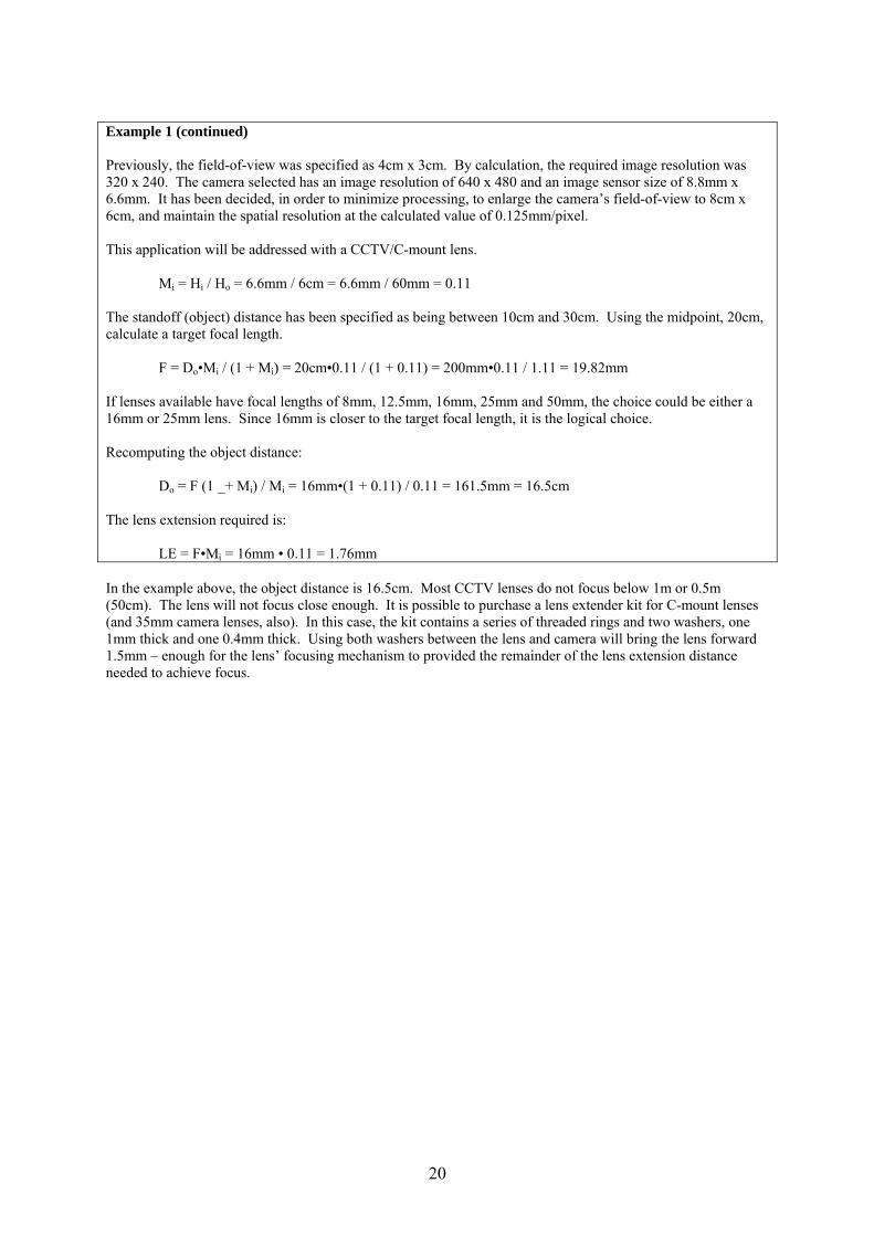
Example 1 (continued) Previously, the field-of-view was specified as 4cm x 3cm. By calculation, the required image resolution was 320 x 240. The camera selected has an image resolution of 640 x 480 and an image sensor size of 8.8mm x 6.6mm. It has been decided, in order to minimize processing, to enlarge the camera’s field-of-view to 8cm x 6cm, and maintain the spatial resolution at the calculated value of 0.125mm/pixel. This application will be addressed with a CCTV/C-mount lens.

Mi = Hi / Ho = 6.6mm / 6cm = 6.6mm / 60mm = 0.11

The standoff (object) distance has been specified as being between 10cm and 30cm. Using the midpoint, 20cm, calculate a target focal length.

F = Do•Mi / (1 + Mi) = 20cm•0.11 / (1 + 0.11) = 200mm•0.11 / 1.11 = 19.82mm If lenses available have focal lengths of 8mm, 12.5mm, 16mm, 25mm and 50mm, the choice could be either a 16mm or 25mm lens. Since 16mm is closer to the target focal length, it is the logical choice. Recomputing the object distance:

Do = F (1 _+ Mi) / Mi = 16mm•(1 + 0.11) / 0.11 = 161.5mm = 16.5cm The lens extension required is:

LE = F•Mi = 16mm • 0.11 = 1.76mm In the example above, the object distance is 16.5cm. Most CCTV lenses do not focus below 1m or 0.5m (50cm). The lens will not focus close enough. It is possible to purchase a lens extender kit for C-mount lenses (and 35mm camera lenses, also). In this case, the kit contains a series of threaded rings and two washers, one 1mm thick and one 0.4mm thick. Using both washers between the lens and camera will bring the lens forward 1.5mm – enough for the lens’ focusing mechanism to provided the remainder of the lens extension distance needed to achieve focus.

20

Example 2 (continued) The field-of-view had been specified as 4cm x 3cm. Previously, the spatial resolution necessary was determined to be .025mm/pixel, and the image resolution to cover this field-of-view at this spatial resolution had been computed as 1600 x 1200 pixels. However, only a very expensive high-resolution area camera would meet this requirement. To continue the example, we will stipulate that the application can be solved with two cameras with image resolutions of 640 x 480 pixels, and an image size of 6.4mm x 4.8mm. Maintaining the spatial resolution at 0.25mm/pixel gives a field-of-view for the cameras of:

FOV (horiz) = Ri (horiz) • Rs = 640 pixels •.025mm/pixel = 16mm FOV (vert) = Ri (vert) • Rs = 480 pixels •.025mm/pixel = 12mm

For this application, enlarger lenses with focusing adaptors will be used. The focal lengths available are 40mm, 60mm, 90mm and 135mm. Standoff distance is specified to be between 40cm and 80cm. First, calculate the magnification.

Mi = Hi / Ho – 4.8mm / 12mm = 0.4. Using a first try object distance of 60cm, calculate the focal length required.

F – Do • Mi / (1 + Mi) = 60cm • 0.4 / (1 + 0.4) = 600mm •0.4 / 1.4 = 171mm The 135mm focal length lens is the closest to this one. Using the lens, compute the object distance.

Do = F (1 + Mi) / Mi = 135mm • (1 + 0.4) / 0.4 = 472.5mm (47.25cm) which is within requirements. Because the application uses a focusing adaptor, it is not necessary to calculate lens extension. In the above example, checking part sizes (cameras and lenses) may show that the two cameras cannot be placed side-by-side. In this case, it would be possible to fold the optical path using mirrors or prisms to allow the cameras to view close together.

21

Example 3 (continued) From previous calculations, the required line-of-view is 20cm. The camera chosen is a line-scan camera with 2,048 elements, an array length of 28.67mm, and a 35mm camera lens mount. There is no standoff distance specified. Lenses are available in focal lengths of 35mm, 50mm, 90mm, and 135mm. Because no standoff (object) distance is specified, select a lens equal to or greater than the image sensor maximum dimension, which for a line-scan sensor is its length. The closest focal length lens to 28.67mm is 35mm. Compute the magnification:

Mi = Hi / Ho = 28.67mm / 20cm = 28.67mm / 200mm = .143 Compute the object distance:

Do = F • (1 + Mi) / Mi = 35mm • (1 +. 143) /.143 = 280mm. The required lens extension to reach focus is:

LE = F • Mi = 35mm -.143 = 5.Omm Since most 35mm camera lenses will focus as close as lm (100 cm), there is no need for additional lens extensions. Select the Lighting Technique The goal of lighting is contrast. In a machine vision image, contrast is the quality of the signal. Contrast is a measure of difference between two regions in the image such as a part and its background. The first step in designing lighting is to determine how the two regions differ. The lighting will be designed to emphasize that difference. The machine vision developer designs lighting by controlling five parameters of light:

Direction - Controlling the direction of incident light is the primary parameter the machine vision developer uses to design illumination. It is controlled by the type and placement of the light sources. Generally, there are two approaches on which all variations are based:

• Directed where the incident light comes virtually from a single direction; it can cast a distinct shadow.

• Diffuse where the incident light comes from many or all directions; it cases very indistinct shadows.

Spectrum - The color of the light. It is controlled by the type of light source and by optical filters over either the light source or the camera lens.

Polarization - The orientation of the waves comprising the illumination. Because specularly reflected light maintains polarization and diffusely reflected light loses polarization, polarized light can be used along with a polarizer over the camera lens (where it is called an analyzer) to eliminate specularly reflected light.

Intensity - The intensity of light affects the camera exposure. The use of insufficient intensity means low contrast or may require the use of additional amplification, which also amplifies noise. The use of excessive intensity results in wasted power and the need to manage excess heat.

Uniformity - In virtually all machine vision applications, uniform illumination is desirable. Since all light sources decrease with distance or angle away from the source, it is often necessary to design illumination as if illuminating a larger area, and only the central region that is relatively uniform illuminates the field-of-view.

22

Some ways in which regions can differ are:

Reflectance - The amount of light reflected from an object that, in the case of machine vision, can be imaged. There are two distinct types of reflections.

Specular or Fresnel reflection is mirror like; the angle of reflection equals the angle of incidence. Specular reflection can be useful or it can produce unwanted glints and glares.

Diffuse reflection is where the incident light is scattered off the object. In a perfect diffuse reflector, light energy is scattered in all directions. In most real situations, the light is scattered over a range of angles dependent on the angle of incidence.

Color -The spectral distribution of light energy that is transmitted or reflected. There are three ways of viewing color. Direct wavelength correlation. For example, light around 550nm wavelength appears green. Additive color where two or more wavelengths of light are combined to produce the effect of a

color not spectrally present. For example, when both yellow light (about 620nm wavelength) and blue light (about 480nm) are present, the combination appears green. Yet there is actually no light energy in the green portion of the spectrum.

Subtractive color where certain wavelengths of light are removed. For example, the difference in a white metal like steel and a yellow metal like gold is not that gold reflects more yellow light than steel, but that it reflects less blue light than steel. White light minus blue light gives the appearance of yellow.

Optical density - The amount of light transmitted by an object may be different due to different materials, different thicknesses, or different chemical properties. The density may be different over the entire spectrum or only at certain points in the optical spectrum. Generally, backlighting is best at detecting differences in optical density.

Refraction - Different transparent materials have different indices of refraction. Thus, they will affect transmitted light in different ways. For example, air and glass have different indices of refraction. Therefore, air bubbles in glass bend the light so as to produce a dark or bright outline of the bubble when illuminated with directional illumination.

Texture - Surface texture may be discernable in the image data, or it may be too fine to be resolved, but affect the reflection. In some cases, texture is important, and must be emphasized with the lighting; other times, texture is unimportant but noise and its effect must be minimized with the lighting.

Height - Differing heights of features on an object may be emphasized with directional illumination (sometimes using shadows) or minimized using very diffuse illumination.

Surface orientation - When surfaces of a part vary depending on their relative orientation, direction light will often allow them to be distinguished; diffuse illumination will often minimize their differences in the image.

There are two general illumination techniques, and several variations within each technique:

Front lighting

Specular - Light is directly reflected off the surface of the part into the camera's lens. Useful for parts where the difference between regions is due to differences in their specular reflection of light. Because every degree of part tilt will move the specularly reflected light by two degrees, this technique is very sensitive to situations where the part pose can change.

Off axis -Light is brought in from the side so that specular reflections are directed away from the cameras, but diffuse reflection reaches the camera. Generally used to cast shadows. Very difficult to accomplish uniform illumination.

Semi-diffuse - Light supplied from a wide range of angles such as from a ring light. Useful where diffusely reflected light is used for imaging. Good uniformity can be achieved in modest sized fields-of-view with reasonable care.

Diffuse -Light supplied from virtually all angles. Useful where the features differ in diffuse reflection and where minimization of specular reflections and variations due to surface orientation are desired.

Dark field - Light supplied from an angle approaching 90 degrees to the camera's viewing direction. Virtually all specular reflection and all diffuse reflection from a flat surface are directed away from the camera. Surface irregularities, such as scratches, provide strong specular glints that can be imaged by the camera.

23

Backlighting

Diffuse - The most common form of backlighting, it consists of a large translucent panel with lights behind it. Easiest to design and achieve reasonable uniformity.

Condenser - Uses a condenser lens to direct the light from the light source into the camera's lens. Useful to create a backlight with directional characteristics.

Dark field - Light supplied from an angle approaching 90 degrees to the camera's viewing direction. Useful when looking for artifacts in transparent materials. With no artifacts present, none of the light reaches the camera. When an artifact is present, some of the light reflects off the artifact into the camera.

The illumination technique should be chosen to take advantage of the difference(s) in the regions to give the greatest possible contrast. In general, backlighting is preferred when the information needed can be obtained from the part or feature's silhouette and where it is mechanically possible to use a backlight. Plan the Image Processing Image processing in machine vision can be modeled in two groups of two steps:

Image simplification - Makes the image less complex. Preprocessing transforms the image into another image that is simpler.

- Point transforms convert each pixel from a source image to a pixel in a destination image. - Neighborhood transforms convert each group of pixels (neighborhood) from a source

image into a pixel value in a destination image. Segmentation divides the image so that each image segment contains only one object or feature.

Image interpretation - Makes sense of the contents of the image. Feature extraction provides information about the image or about objects or features in the image.

- Statistical features, like average gray level or pixel count, tend to be robust but of low precision.

- Geometric features, like dimensions, tend to be precise, but can be more easily corrupted by image artifacts.

Interpretation determines from the features extracted what the system should output (e.g., whether the part is good or bad).

- Statistical techniques, like linear classifiers, tend to be robust, but most useful for categorizing data in applications like part recognition or OCR.

- Deterministic techniques, like decision trees, tend to be more precise, and are useful when precision measurements are involved.

As a general approach, the developer should work backward - from the known specified goal state to the unknown incoming image. That is, the developer will first pick an interpretation technique that is suitable for the output required, and then identify features which can be expected to be available from the image and which will support the interpretation technique. After features are identified, image simplification can be addressed. If multiple parts are present in the image or the part has multiple features, segmentation may likely be required. The segmentation technique can be picked. Finally, any preprocessing expected can be identified. One general guideline has proven effective: avoid image simplification, preprocessing and segmentation, if at all possible. Many times, front-end work on lighting and optics can yield a high quality image, one with high contrast and low noise, which eliminates or minimizes the need for preprocessing. Likewise, designing the way parts are presented to the camera can help eliminate the need for segmentation. Preprocessing, especially neighborhood processes, are computationally expensive. As computers get faster, the cost in time for preprocessing comes down. But at the same time, image resolution is increasing, and this increases the preprocessing computational burden. Segmentation can be troublesome, especially for touching and overlapping parts. Recent progress with shape based recognition and segmentation is helping improve the reliability of segmentation, but it comes at a price of substantially increased processing burden.

24

Choose the Software Package When choosing a software package, look for these attributes:

Functionality - The software package must support the planned image processing functions or their equivalent.

Level of integration Application specific - Tailored to performing a specific function (e.g., measurement). No

programming required; the developer simply configures the software to meet application requirements.

General purpose - The software package is complete including a range of image processing functions and a configurable user interface. It requires more configuration work than an application specific package, but little or no programming to use.

API (application programming interface) - This is a library of functions, usually comprising image processing functions. The developer must write software to create the user interface and invoke the desired image processing functions.

Hardware compatibility - The software package must be compatible with the operating system and related hardware such as the frame grabber and camera. It supplies driver software for the frame grabber and may have functions that control special camera features.

Development support - The software package must provide support to facilitate development. The development environment may require special hardware or software not necessary for the final installation.

Technical support - It is inevitable that some technical support on the software package will benefit the project. Know how the supplier provides this support and the level of competence of the support staff.

Proving Feasibility Proving feasibility is a must in machine vision development. If the technology and application closely resemble an existing system, and if that system design can be copied with minor modifications, then a feasibility study is not needed. Otherwise, a feasibility study is an absolutely necessary part of a machine vision project. The goals of a machine vision feasibility study are:

Prove acceptable image quality Provide a test environment to work through any image processing questions Verify operational speed if that is in question Provide a test environment to develop equipment interfaces if there are substantial questions

Needed for the feasibility study are:

The exact lighting and optics components expected for the final system A good set of samples Image processing capability as necessary Simulation of part handling if necessary

Finally, the need to document the feasibility study with hard data as well as pictorially (sketches and photographs work well) cannot be overstressed. Many times, once a system is built, it does not replicate the feasibility test results. Only by reviewing the documentation of the study can the differences be identified and corrective action initiated.

25

Making the Vision System Bomb Proof By the time the detailed system design is started, most of the machine vision specific engineering is complete and proven. However, there are a number of threats unique to machine vision systems which need to be addressed in the detailed system design. These are:

Alignment Maintainability Calibration Part motion Shock and vibration Cold Heat Humidity Airborne hazards Electrical interference

Alignment The main challenge of alignment in a vision system is the development of an efficient method of adjusting the position of the camera and light position. Generally, sound mechanical design principles are all that are needed. The developer should recognize that every object (e.g., camera or light source) has six potential degrees of freedom. In practice, some of the degrees of freedom will not matter. For example, when looking at the end of an incandescent lamp, roll (rotation about the longitudinal axis) does not matter. Naturally, any degree of motion that does not matter can be ignored. Also, a part's position in certain directions or rotations may have such great tolerance that no provision for adjustment is needed. For those degrees of freedom which are critical, each should have only one adjustment. To the degree practical, the adjustments should not interact, and each adjustment should be robust and be able to be securely locked. For example, if a camera is to be adjusted in roll, pitch and yaw, these motions ideally will all pivot about the front nodal point of the lens to avoid interaction. (The front nodal point of the lens is the center of the lens' front principal plane.) As a practical matter, most lenses do not come with information about the location of the front nodal point. Even if the front nodal point were known, the camera would need to be mounted on a complex gimble system to achieve the desired motion. A more practical design would be to use a pivot (e.g., a ball bearing) in a convenient location as near to the estimated nodal point as possible. Positioning the camera will involve some degree of interaction between the different adjustments, but the simplicity of the mount will be much superior. Also the rigidity of the mount and the ability to securely lock down the adjustments will be enhanced. In summary, the considerations in designing for alignment are:

Eliminate as many degrees of freedom from needing adjusting as possible Have only one adjustment per degree of freedom Minimize the interaction of the adjustments consistent with good and practical design Make the adjustments readily accessible to maintenance people, but not necessarily to operators

A final note is that many machine vision practitioners have found it advantageous to assemble a camera and its associated optics and lighting into a single module, called an optical head, which can be prealigned before mounting into the machine vision system. Maintainability On the whole, vision systems are very reliable. However, there are components, like lamps, which can be expected to need periodic replacement. A good system design will anticipate which components need replacement, make sure those components are readily accessible to maintenance personnel, and when replaced, require a minimum of alignment and calibration to return the system to service.

26

Calibration Calibration can have up to three functions:

Determination of spatial resolution Determination of the location of the camera with reference to some base coordinate system Determination of color balance

There are three basic options:

No calibration needed. For example, in a system that determines the number of holes in a part, no dimensional or color information is needed; therefore, calibration is not necessary.

Use of a golden part or transfer standard. Many measurement systems are calibrated using a standard (e.g., gage block) or golden part that has traceability to NIST or other standard setting agency.

Use of objects permanently fixtured in the field-of-view which themselves have known, calibrated characteristics. For example, some color-based systems use a small white tile in a corner of the field-of-view to provide a color standard for color balance calibration with every image.

There are two scopes of calibration:

Single point - The system is calibrated at one point in the image, usually the center, and that information is taken as valid across the image.

Multiple point - The system is calibrated at many points within the image (usually on a regular grid), and the calibration for any location is determined from this array either through a look-up table or through an equation fit to the set of data points.

The second scope of calibration is naturally much more complex, but in situations which demand the most from a vision system, it is usually necessary. Part Motion The main concern with part motion is a blurry image, and in some cases with parts moving at high speeds, capturing an image with the entire part in view. When parts are not stationary during imaging, the effects of motion need to be considered, and in many cases mitigated. For line-scan cameras, part motion may be an integral component of successful imaging. However, since each scan line is imaging a moving part, there will be a dynamic component - an inevitable blurring in the direction of part motion. The effect might be to reduce effective resolution in that direction. If this is a problem, the only practical remedy is to increase the scan rate. This has two drawbacks. One is the increase in incoming pixel data rate. The second is an increase in light intensity needed to maintain exposure. When using area cameras, even seemingly small motions can degrade the image. Use of a progressive scan camera is almost mandatory. Interlaced cameras acquire the two fields at different times. The effect will be a picket fence like appearance on vertical edges. When using area cameras, the use of an electronic shutter, a feature on many cameras, is an option. Electronic shutters operate in as little as a fraction of a millisecond. One consideration in using electronic shutters is the need to increase illumination intensity to compensate for the reduced exposure time. Another consideration when using electronic shutters is the timing of the shutter with part position. With synchronous (free running) cameras, there are restrictions on when the shutter will operate. Asynchronous or triggered cameras are available in which the image acquisition, and therefore the shutter timing, can be coordinated to the part's arrival. The special cameras place demands on the frame grabber, and will narrow the selection options to fewer, more sophisticated, and more expensive frame grabbers. Another common technique for freezing part motion is to use strobed illumination. Xenon strobe lamps have been used for many years, and have a light pulse width of as little as a few microseconds. Within the past few years, pulsed LED light sources have become available. The LED light sources are good for smaller fields-of-view, have long life, and have pulses as short as a fraction of a millisecond. For most cameras, there is a time window in which the strobe can be fired, and a period of time each frame (or field) period where the strobe cannot be fired (to have a quality image). The use of strobed illumination places similar demands on the frame

27

grabber as when electronic shutters are used, except the frame grabber must also have a strobe output trigger that is compatible with the needs of the camera. Use of strobe light sources present the need to consider human factors. Flashing lights can be annoying to work around and at some flash rates can even induce seizures in certain people. Shock and Vibration The biggest concerns with mechanical shock and vibration are loss of alignment and calibration and premature component failure. Image degradation from blurring is also a concern. Of course, one obvious remedy is to eliminate the cause or possibility of shock and vibration. When that is not practical, the second choice is to mechanically isolate the system components from vibration and to use mechanical dampening. Protect the vision system components from mechanical shock by placing barriers to protect it from impact. A final element of the remedy is to pick components that are more resistant to shock and vibration. Many cameras have their genealogy in surveillance applications, and are not designed to withstand harsh mechanical environments. Some cameras have been specifically designed for the industrial environment, and have specifications for their ability to withstand shock and vibration. When choosing lamps, give preference to rugged light sources like LEDs. When incandescent lamps must be used, choose low voltage lamps that have thicker, stronger filaments than equivalent high voltage bulbs. Cold The principal concern with cold temperature is the potential for condensation, especially on optical surfaces. When the vision system is expected to be in a relatively cold environment or when the temperature might drop rapidly, condensation can be prevented by using heating elements to keep the temperature of the external components warm enough to prevent condensation. The interiors of enclosures can also be purged with filtered and dried air. Heat The principal concern with heat is the failure of components. An additional concern is the increase in image noise, especially from the camera's image sensor. The rule of thumb is that each 7°C rise in temperature reduces an electrical component's life by one-half. Of course, extreme temperatures can destroy components. Using convection cooling or refrigeration can mitigate the effects of heat. For extreme temperatures such as those encountered in steel mills, components can be mounted in water-cooled enclosures. Humidity As with cold temperatures, the chief concern with high humidity is the potential for condensation, especially on optical surfaces. The remedies are the same as for cold temperature: warm the vision system components to a temperature slightly above ambient, and keep a curtain of dry air flowing across critical components. Airborne Hazards Airborne hazards like dust, mist, and flying debris pose a real threat for image degradation when there is the potential for them to land on or stick to optical surfaces. The solutions are either to remove the critical vision components away from where the airborne hazards are present, or use a clean dry air purge around the optics. Tins air purge cannot be turbulent; turbulent air has the potential for moving contaminated air into contact with the optical surfaces.

28

Electrical interference The biggest concerns with electrical interference are the potential for component damage and for unreliable system operation. Electrical interference can come from power line fluctuations, electrical spikes conducted through the power lines, and radiated energy from other equipment. The best protection against electrical interference is good shielding and grounding. Good grounding procedures must be followed to prevent ground loops which can pose a serious problems. Also, consider conditioning the incoming power to filter out conducted noise and, where required, to regulate the line voltage.

29

Specification Outline General Description of Project

Description of the Operation Present Method of Operation (if any) Need(s) to be met Source(s) of Cost Savings Anticipated Increased Cost(s) Number of Workers Displaced Desirability of Jobs Displaced Subsidiary Tasks Performed by Present Workers and Proposed Method of Fulfilling Subsidiary

Tasks Objects to be Viewed

Number of Different Parts Future Increases in Number of Parts Description of Object(s) Variations in Each Object Type Size Colour(s) of Object(s) Surface Condition of Object(s)

- Surface Finish - Corrosion - Lubricants/Rust Inhibitors - Dirt

Perishability Sensitivity to Heat Damage from Lamp Change in Object(s) Appearance Due to Defects/Damage

- Insignificant Appearance Changes - Significant Appearance Changes

Performance Requirements

Data to be Extracted from the Image Accuracy Process Reliability Equipment Reliability Response Triggered with no Part in View Production Rate (Seconds/Part or Inches/Second)

Part Presentation

Part Motion Continuous Indexed Hand loaded Rate of Travel or Dwell Time Part Registration Batch Production Yes No Mixed Party Types Yes No Number of Parts in View at One Time Touching/Overlapping Parts Touching Overlapping Vertical Motion Movement During Viewing

30

Optical Requirements

Field-of-view Depth-of-view Standoff Distance

- Camera - Light Source

Backlighting Possible Yes No Front Lighting Possible Yes No

Physical

Mounting and Access - Camera - Light Source - Processor

Distance Between Camera and Processor Required Packaging Retrofit/New Design Retrofit New Design

Utilities Available

Electrical Power - Voltage(s) - Maximum Current

Compressed Air - Pressure - Maximum Flow - Temperature

Vacuum Cooling Water

- Pressure - Maximum Flow - Temperature

Environment

Physical - Shock - Vibration - Hazards from Equipment/Process Malfunctions - Temperature Range - Flying Debris - Plant Cleaning Procedures

Optical and Electrical - Ambient Light - Electromagnetic Interference - Radio Frequency Interference - Electrical Power Regulation

Atmosphere - Humidity - Dust - Mist - Corrosive Fumes - Radiation

31

Interface with Production Process Equipment

Interconnected Equipment Communication Protocol(s) Trigger Signal Data Log

Operator Interface

Controls Report Generation Programming Set-up and Calibration

Support Requirements

Application Software Material Handling Optical Design System Installation Training Service

- Spare Inventory - Service Personnel

Future Modifications

32

Machine Vision Integration Pre-Launch Checklist

Champion Name: _______________________________________________________________ Available Committed Energetic Leader Managerial Support Project addresses major goal Meets investment criteria Proposal submitted Resources available Project Team (enter name or “not needed” as appropriate) Project management: ___________________________________________________ Process engineering: ___________________________________________________ Part handling: _________________________________________________________ Equipment packaging: __________________________________________________ Optics: ______________________________________________________________ Electronics: __________________________________________________________ Software: ____________________________________________________________ Training: _____________________________________________________________ Maintenance: _________________________________________________________ Specification Available and complete Acceptance Test Available and complete Sample Set Number of Samples: Calibrated Adequately represents range of parts

33

Machine Vision System Initial Design Worksheet

Camera Type: Area Line-scan Number of Cameras: ______________________ Field-of-view: Camera 1 Camera 2 Camera 3 ____________________ ____________________ ____________________ Resolution: Requirements:

Feature resolution (if required):

- Minimum feature size: _________________________

- Pixels spanning minimum feature: _________________________

Measurement resolutions (if required):

- Measurement precision required: ________________________

- Vision system measurement precision: ____________________ pixel

Spatial resolution required (from above): ____________________ (unit/pixel)

Image resolution: ______________ (columns x______________ (rows) pixels

Spatial resolution available from field-of-view and image resolution:

___________________ (unit/pixel)

Computational burden: __________________ pixels/second Lens selection: Standoff distance range: _______________________ Lens focus length: ____________________ mm

34

Machine Vision System – Initial Design Worksheet (continued) Contrast: Feature Background Lighting Filter

Noise: Source Expected magnitude Mitigation

Processing: Goal: ________________________________________________________________ Interpretation: _________________________________________________________ Features: _____________________________________________________________ Segmentation (if necessary): _____________________________________________ Preprocessing (if necessary): _____________________________________________ Alignment: Brief description of alignment procedures attached Calibration: Transfer standards Fixed calibration targets No calibration required Brief description of calibration procedures attached

35