Advanced Fluid Mechanics 2016 Prof P.C.Swain Page 1 MCE2121 ADVANCED FLUID MECHANICS LECTURE NOTES Module-I Department Of Civil Engineering VSSUT, Burla Prepared By Dr. Prakash Chandra Swain Professor in Civil Engineering Veer Surendra Sai University of Technology, Burla Branch - Civil Engineering Specialization-Water Resources Engineering Semester – 1 st Sem

Welcome message from author
This document is posted to help you gain knowledge. Please leave a comment to let me know what you think about it! Share it to your friends and learn new things together.
Transcript

Advanced Fluid Mechanics 2016
Prof P.C.Swain Page 1
MCE2121
ADVANCED FLUID MECHANICS
LECTURE NOTES
Module-I
Department Of Civil Engineering
VSSUT, Burla
Prepared By
Dr. Prakash Chandra Swain
Professor in Civil Engineering
Veer Surendra Sai University of Technology, Burla
Branch - Civil Engineering
Specialization-Water Resources Engineering
Semester – 1st Sem

Advanced Fluid Mechanics 2016
Prof P.C.Swain Page 2
Disclaimer
This document does not claim any originality and cannot be
used as a substitute for prescribed textbooks. The information
presented here is merely a collection by Prof. P.C.Swain with
the inputs of Post Graduate students for their respective
teaching assignments as an additional tool for the teaching-
learning process. Various sources as mentioned at the
reference of the document as well as freely available materials
from internet were consulted for preparing this document.
Further, this document is not intended to be used for
commercial purpose and the authors are not accountable for
any issues, legal or otherwise, arising out of use of this
document. The authors make no representations or warranties
with respect to the accuracy or completeness of the contents of
this document and specifically disclaim any implied warranties
of merchantability or fitness for a particular purpose.

Advanced Fluid Mechanics 2016
Prof P.C.Swain Page 3
Course Content
Module I
Introduction: Survey of Fluid Mechanics, Structure of Fluid
Mechanics Based on Rheological, Temporal Variation, Fluid Type,
Motion Characteristic and spatial Dimensionality Consideration,
Approaches in Solving Fluid Flow Problems, Fundamental
idealizations and Descriptions of Fluid Motion, Quantitative
Definition of Fluid and Flow, Reynolds Transport Theorem, Mass,
Momentum and Energy Conservation Principles for Fluid Flow.
Potential Flow: Frictionless Irrotational Motions, 2 - Dimensional
Stream Function and Velocity Potential Function in Cartesian and
Cylindrical Polar Coordinate Systems, Standard Patterns of Flow,
Source, Sink, Uniform Flow and irrotational vortex, Combinations of
Flow Patterns, method of Images in Solving Groundwater Flow
problems, Method of Conformal transformations.

Advance Fluid Mechanics 2016
Prof P.C Swain Page 1
MODULE-I
Lecture Note 1
INTRODUCTION
Fluid is a substance that continually deforms (flows) under an applied shear stress. Fluids are a
subset of the phases of matter and include liquids, gases, plasmas and, to some extent, plastic
solids. Fluids are substances that have zero shear modulus or, in simpler terms, a fluid is a
substance which cannot resist any shear force applied to it.
Fluid mechanics is the branch of science which deals with the behavior of fluids(liquids or
gases)at rest as well as in motion. It deals with the static, kinematics and dynamic aspects of
fluids.
The study of fluids at rest is called fluid statics. The study of fluid in motion is called fluid
kinematics if pressure forces are not considered if pressure force is considered in fluid in motion
is called fluid dynamics.
PROPERTIES OF FLUIDS
DENSITY or MASS DENSITY:-
The density, or more precisely, the volumetric mass density, of a substance is its mass per unit
volume. The symbol most often used for density is ρ( Greek letter rho), Mathematically, density
is defined as mass divided by volume
ρ=m
V
whereρ is the density, m is the mass, and V is the volume. In some cases (for instance, in the
United States oil and gas industry), density is loosely defined as its weight per unit volume.

Advance Fluid Mechanics 2016
Prof P.C Swain Page 2
SPECIFIC WEIGHT or WEIGHT DENSITY:-
The specific weight (also known as the unit weight) is the weightper unit volume of a material. It
is denoted as the symbol w. Mathematically,
w =weight of fluid
Volume of fluid
=mass of fluid∗acceleration due to gravity
Volume of fluid
= m
V∗ 𝑔
= ρg
SPECIFIC GRAVITY:-
It is defined as the ratio of the weight density of a fluid to weight density of a standard fluid. For
liquids the standard fluid is taken as water and for gases the standard fluid is given as air. It is
denoted as S.
S(for liquids)=Weight density of liquid
weight density of water
S(for gases)=Weight density of gases
weight density of air
COMPRESSIBILITY:-
Compressibility is a measure of the relative volume change of a fluid or solidas a response to a
pressure (or mean stress) change.
β= -𝑑𝑣
𝑣𝑑𝑝
whereV is volume and p is pressure.

Advance Fluid Mechanics 2016
Prof P.C Swain Page 3
ELASTICITY:-
Elasticity is the ability of a body to resist a distorting influence or stress and to return to its
original size and shape when the stress is removed. Solid objects will deform when forces are
applied on them. If the material is elastic, the object will return to its initial shape and size when
these forces are removed.
SURFACE TENSION:-
It is defined as the tensile force acting on the surface of a liquid in contact with a gas or on the
surface between two immiscible liquids such that the contact surface behaves like a membrane
under tension. The magnitude of this force per unit length of the free surface will have the same
value as the surface energy per unit area. It is denoted as 𝜎 (called sigma).Unit is N/m.
CAPILLARITY:-
Capillarity is defined as a phenomenon of rise or fall of a liquid surface in small tube relative to
the adjacent general level of liquid when the tube is held vertically in the liquid. The rise of
liquid surface is known as capillary rise while the fall of liquid surface is known as capillary
depression. It is expressed in terms of cm or mm of liquid. Its value depends upon the specific
weight of the liquid, diameter of the tube and surface tension of the liquid.

Advance Fluid Mechanics 2016
Prof P.C Swain Page 4
VISCOSITY:-
It is defined as the property of a fluid which offers resistance to the movement of one layer of
fluid over another adjacent layer of the fluid. When two layers of a fluid, a distance ‘dy’ apart ,
move one over the other at different velocities, say u and u+du.
Newton’s law of Viscosity:-
It states that the shear stress on a fluid element layer is directly proportional to the rate of shear
strain. The constant of proportionality is called the coefficient of viscosity. Mathematically,
𝜏 = 𝜇𝑑𝑢
𝑑𝑦
Advance Fluid Mechanics 2016
Prof P.C Swain Page 5
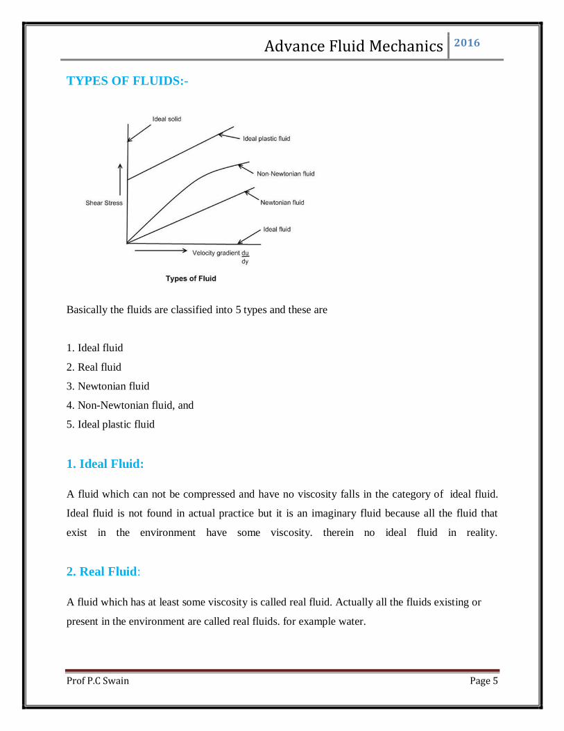
TYPES OF FLUIDS:-
Basically the fluids are classified into 5 types and these are
1. Ideal fluid
2. Real fluid
3. Newtonian fluid
4. Non-Newtonian fluid, and
5. Ideal plastic fluid
1. Ideal Fluid:
A fluid which can not be compressed and have no viscosity falls in the category of ideal fluid.
Ideal fluid is not found in actual practice but it is an imaginary fluid because all the fluid that
exist in the environment have some viscosity. therein no ideal fluid in reality.
2. Real Fluid:
A fluid which has at least some viscosity is called real fluid. Actually all the fluids existing or
present in the environment are called real fluids. for example water.
Advance Fluid Mechanics 2016
Prof P.C Swain Page 6
3. Newtonian Fluid:
If a real fluid obeys the Newton's law of viscosity (i.e the shear stress is directly proportional to
the shear strain) then it is known as the Newtonian fluid.
4. Non-Newtonian Fluid:
If real fluid does not obeys the Newton's law of viscosity then it is called Non-Newtonian fluid.
5. Ideal Plastic Fluid:
A fluid having the value of shear stress more than the yield value and shear stress is proportional
to the shear strain (velocity gradient) is known as ideal plastic fluid.
MANOMETER:-
A manometer is an instrument that uses a column of liquid to measure pressure, although the
term is currently often used to mean any pressure instrument. Two types of manometer.
1.Simple manometer
2.Differential manometer
The U type manometer, which is considered as a primary pressure standard, derives pressure
utilizing the following equation:
P = P2 - P1 = h𝜔 ρg
Where:
P = Differential pressure
P1 = Pressure applied to the low pressure connection
P2 = Pressure applied to the high pressure connection
h𝜔 = is the height differential of the liquid columns between the two legs of the manometer
ρ = mass density of the fluid within the columns
g = acceleration of gravity

Advance Fluid Mechanics 2016
Prof P.C Swain Page 7
Simple manometer:-
A simple manometer consists of a glass tube having one of its ends connected to a point where
pressure is to be measured and other end remains open to atmosphere. Common types of simple
manometers are:
1.Piezometer
2.U tube manometer
3.Single Column manometer
PIEZOMETER
A piezometer is either a device used to measure liquid pressure in a system by measuring the
height to which a column of the liquid rises against gravity, or a device which measures the
pressure (more precisely, the piezometric head) of groundwaterat a specific point. A piezometer
is designed to measure static pressures, and thus differs from a pitot tube by not being pointed
into the fluid flow.

Advance Fluid Mechanics 2016
Prof P.C Swain Page 8
U TUBE MANOMETER-
Manometers are devices in which columns of a suitable liquid are used to measure the difference
in pressure between two points or between a certain point and the atmosphere.
Manometer is needed for measuring large gauge pressures. It is basically the modified form of
the piezometric tube. A common type manometer is like a transparent "U-tube" as shown in Fig.
simple manometer to measure gauge pressure

Advance Fluid Mechanics 2016
Prof P.C Swain Page 9
simple manometer to measure vacuum pressure
SINGLE COLUMN MANOMETER:-
It is a modified form of a U tube manometer in which a reservoir having a large cross sectional
area.
DIFFERENTIAL MANOMETER:-
Differential Manometers are devices used for measuring the difference of pressure between two
points in a pipe or in two different pipes . A differential manometer consists of a U-tube,
containing a heavy liquid, whose two ends are connected to the points, which difference of
pressure is to be measure.
Most commonly types of differential manometers are:
1- U-tube differential manometer.

Advance Fluid Mechanics 2016
Prof P.C Swain Page 10
2- Inverted U-tube differential manometer
U-tube differential manometer.
For two pipes are at same levels:-
PA-PB=h.g(pg-p1)
Where:
P1=density of liquid at A=density of liquid at B.
For two pipes are in different level:-
PA- PB= h.g (pg-p1) + p2gy- p1 gx
Where:
h = difference in mercury level in the U-tube
y = distance of the centre of B, from the mercury level in the right limb.
x = distance of the centre of A, from the mercury level in the left limb. P1=density of liquid
at A.
p2=density of liquid at B.
pg=density of mercury (heavy liquid)
Inverted U-tube differential manometer
Advance Fluid Mechanics 2016
Prof P.C Swain Page 11
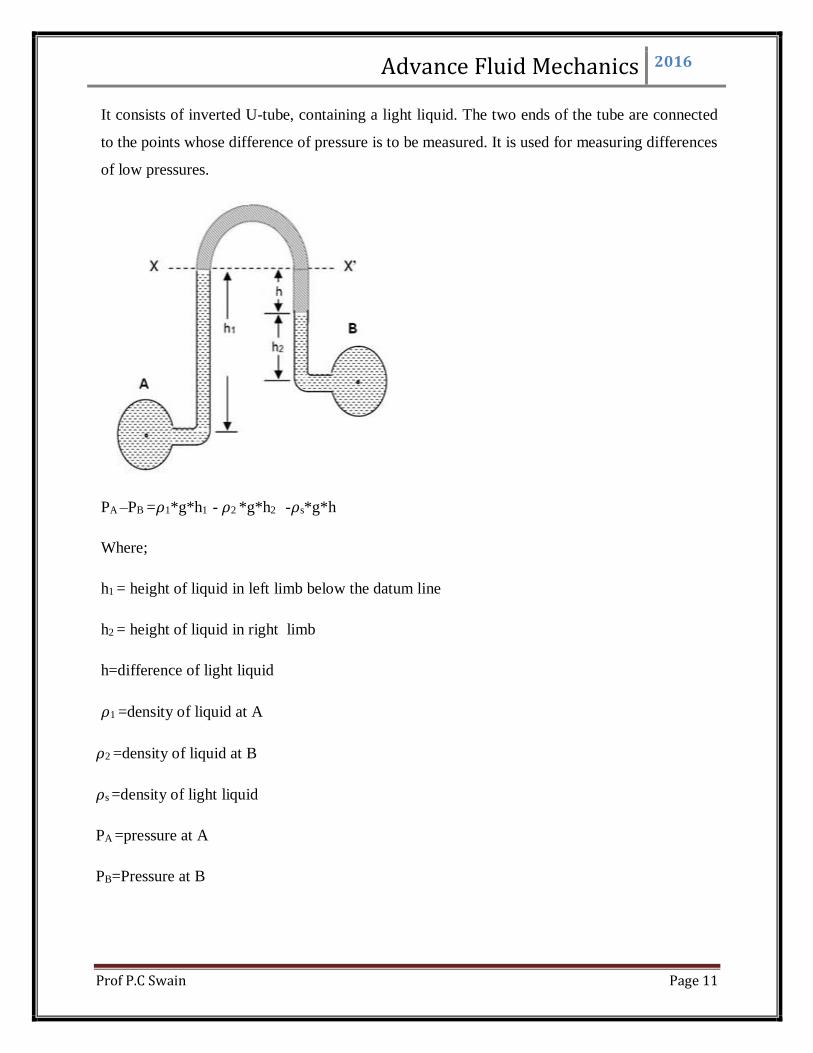
It consists of inverted U-tube, containing a light liquid. The two ends of the tube are connected
to the points whose difference of pressure is to be measured. It is used for measuring differences
of low pressures.
PA –PB =𝜌1*g*h1 - 𝜌2 *g*h2 -𝜌s*g*h
Where;
h1 = height of liquid in left limb below the datum line
h2 = height of liquid in right limb
h=difference of light liquid
𝜌1 =density of liquid at A
𝜌2 =density of liquid at B
𝜌s =density of light liquid
PA =pressure at A
PB=Pressure at B

Advance Fluid Mechanics 2016
Prof P.C Swain Page 12
Buoyancy
When a body is either wholly or partially immersed in a fluid, a lift is generated due to
the net vertical component of hydrostatic pressure forces experienced by the body.
This lift is called the buoyant force and the phenomenon is called buoyancy
Consider a solid body of arbitrary shape completely submerged in a homogeneous liquid
as shown in Fig. Hydrostatic pressure forces act on the entire surface of the body.
Stability of Floating Bodies in Fluid
When the body undergoes an angular displacement about a horizontal axis, the shape of
the immersed volume changes and so the centre of buoyancy moves relative to the body.
As a result of above observation stable equilibrium can be achieved, under certain
condition, even when G is above B. Fig illustrates a floating body -a boat, for example,
in its equilibrium position.

Advance Fluid Mechanics 2016
Prof P.C Swain Page 13
Important points to note here are
a. The force of buoyancy FB is equal to the weight of the body W
b. Centre of gravity G is above the centre of buoyancy in the same vertical line.
c. Figure b shows the situation after the body has undergone a small angular displacement q
with respect to the vertical axis.
d. The centre of gravity G remains unchanged relative to the body (This is not always true
for ships where some of the cargo may shift during an angular displacement).
e. During the movement, the volume immersed on the right hand side increases while that
on the left hand side decreases. Therefore the centre of buoyancy moves towards the right
to its new position B'.
Let the new line of action of the buoyant force (which is always vertical) through B' intersects
the axis BG (the old vertical line containing the centre of gravity G and the old centre of
buoyancy B) at M. For small values of q the point Impractically constant in position and is
known as metacentre. For the body shown in Fig. M is above G, and the couple acting on the
body in its displaced position is a restoring couple which tends to turn the body to its original
position. If M were below G, the couple would be an overturning couple and the original
equilibrium would have been unstable. When M coincides with G, the body will assume its new
position without any further movement and thus will be in neutral equilibrium. Therefore, for a
Advance Fluid Mechanics 2016
Prof P.C Swain Page 14
floating body, the stability is determined not simply by the relative position of B and G,ratherby
the relative position of M and G. The distance of metacentre above G along the line BG is known
as metacentric height GM which can be written as
GM = BM -BG
Hence the condition of stable equilibrium for a floating bodycan be expressed in terms
ofmetacentric heightas follows:
GM > 0 (M is above G) Stable equilibrium
GM = 0 (M coinciding with G) Neutral equilibrium
GM < 0 (M is below G) Unstable equilibrium
The angular displacement of a boat or ship about its longitudinal axis is known as 'rolling' while
that about its transverse axis is known as "pitching".
Hydrostatic Thrusts on Submerged Plane Surface
Due to the existence of hydrostatic pressure in a fluid mass, a normal force is exerted on any part
of a solid surface which is in contact with a fluid. The individual forces distributed over an area
give rise to a resultant force.
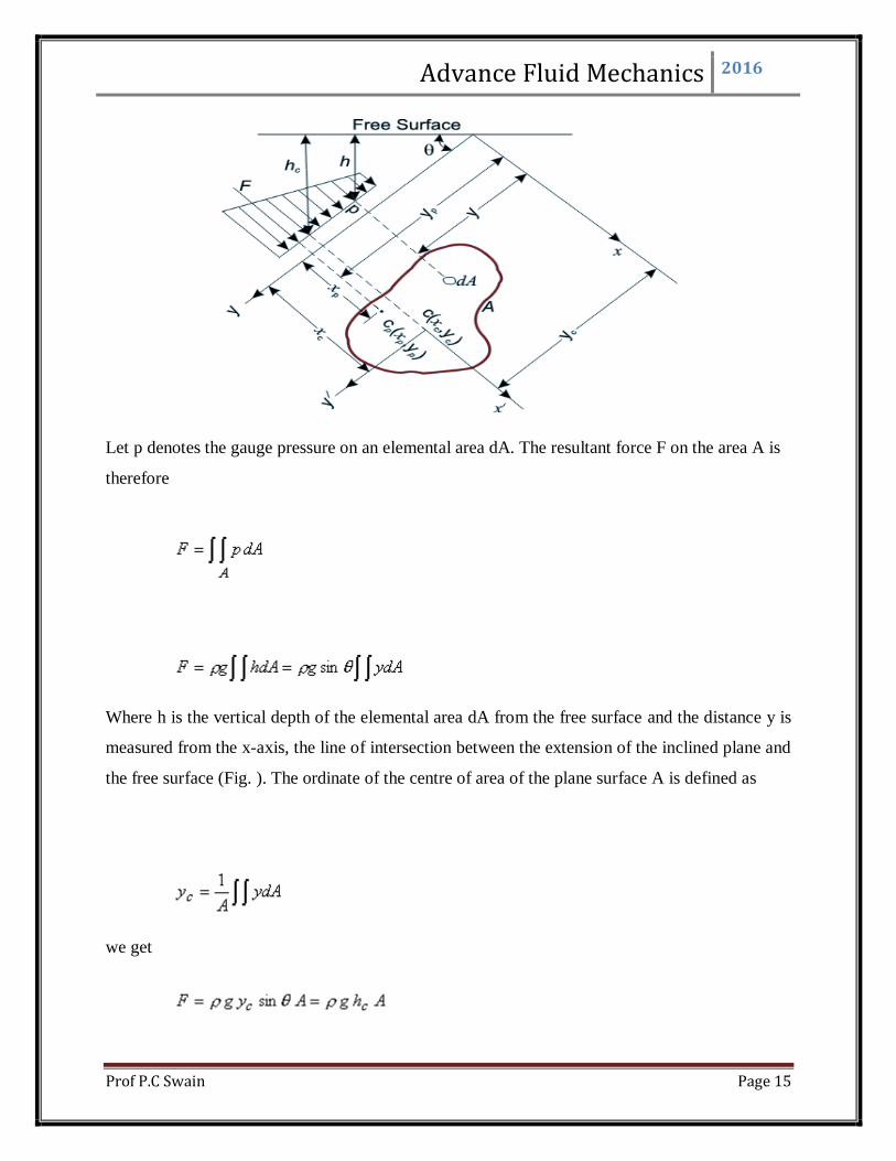
Plane Surfaces
Consider a plane surface of arbitrary shape wholly submerged in a liquid so that the plane of the
surface makes an angle θ with the free surface of the liquid. We will assume the case where the
surface shown in the figure below is subjected to hydrostatic pressure on one side and
atmospheric pressure on the other side.
Advance Fluid Mechanics 2016
Prof P.C Swain Page 15
Let p denotes the gauge pressure on an elemental area dA. The resultant force F on the area A is
therefore
Where h is the vertical depth of the elemental area dA from the free surface and the distance y is
measured from the x-axis, the line of intersection between the extension of the inclined plane and
the free surface (Fig. ). The ordinate of the centre of area of the plane surface A is defined as
we get

Advance Fluid Mechanics 2016
Prof P.C Swain Page 16
where is the vertical depth (from free surface) of centre c of area .
Hydrostatic Thrusts on Submerged Curved Surfaces
On a curved surface, the direction of the normal changes from point to point, and hence the
pressure forces on individual elemental surfaces differ in their directions. Therefore, a scalar
summation of them cannot be made. Instead, the resultant thrusts in certain directions are to be
determined and these forces may then be combined vectorially. An arbitrary submerged curved
surface is shown in Fig. A rectangular Cartesian coordinate system is introduced whose xy plane
coincides with the free surface of the liquid and z-axis is directed downward below the x - y
plane.
Consider an elemental area dA at a depth z from the surface of the liquid. The hydrostatic force
on the elemental area dA is
Advance Fluid Mechanics 2016
Prof P.C Swain Page 17
and the force acts in a direction normal to the area dA. The components of the force dF in x, y
and z directions are
Where l, m and n are the direction cosines of the normal to dA. The components of the surface
element dA projected on yz, xz and xy planes are, respectively
From equations,
Therefore, the components of the total hydrostatic force along the coordinate axes are

Advance Fluid Mechanics 2016
Prof P.C Swain Page 18
wherezc is the z coordinate of the centroid of area Ax and Ay (the projected areas of curved
surface on yz and xz plane respectively). If zp and yp are taken to be the coordinates of the point
of action of Fx on the projected area Ax on yz plane, , we can write
whereIyy is the moment of inertia of area Ax about y-axis and Iyz is the product of inertia of Ax
with respect to axes y and z. In the similar fashion, zp' and xp
' the coordinates of the point of
action of the force Fy on area Ay, can be written as
whereIxx is the moment of inertia of area Ay about x axis andIxz is the product of inertia of Ay
about the axes x and z.
We can conclude from previous Eqs that for a curved surface, the component of hydrostatic force
in a horizontal direction is equal to the hydrostatic force on the projected plane surface
perpendicular to that direction and acts through the centre of pressure of the projected area. From
Eq. the vertical component of the hydrostatic force on the curved surface can be written as
Where is the volume of the body of liquid within the region extending vertically above the
submerged surface to the free surface of the liquid. Therefore, the vertical component of
hydrostatic force on a submerged curved surface is equal to the weight of the liquid volume
Advance Fluid Mechanics 2016
Prof P.C Swain Page 19
vertically above the solid surface of the liquid and acts through the center of gravity of the liquid
in that volume.
Derivation of Reynolds Transport Theorem
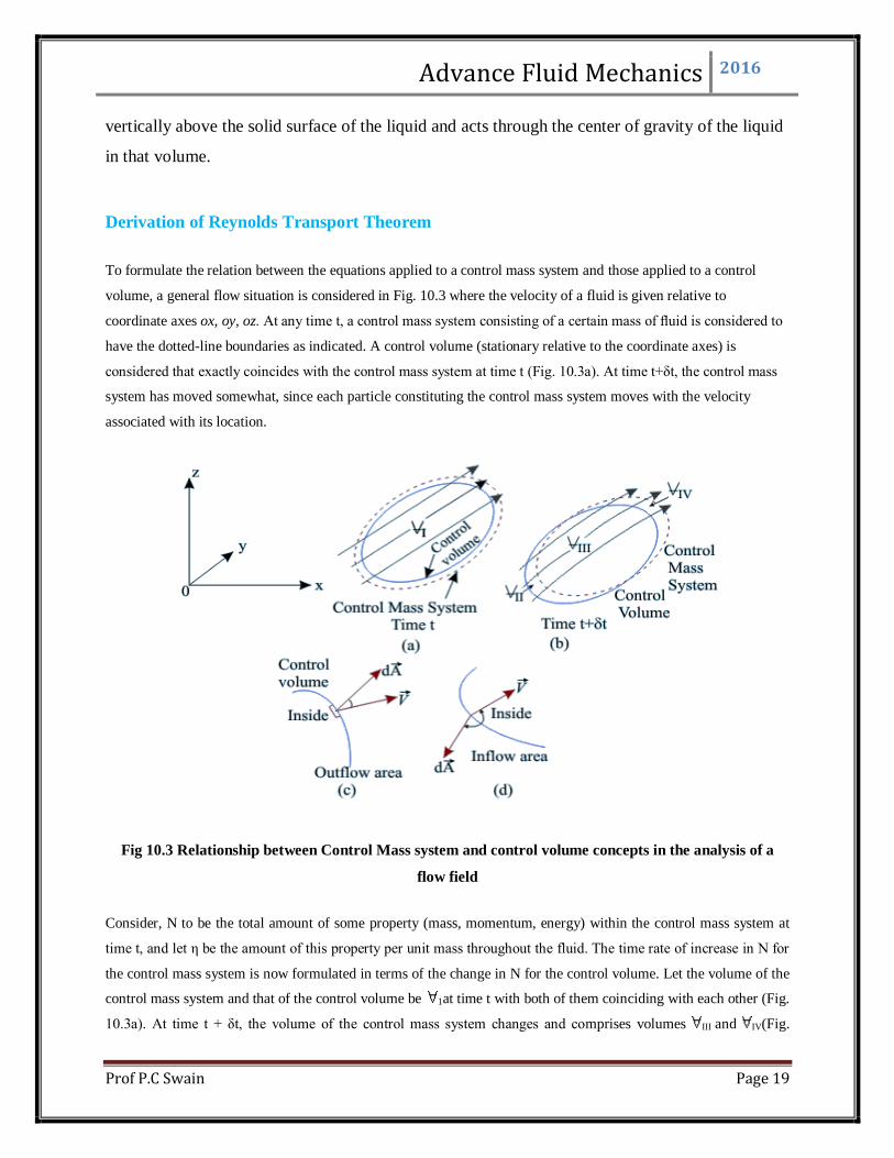
To formulate the relation between the equations applied to a control mass system and those applied to a control
volume, a general flow situation is considered in Fig. 10.3 where the velocity of a fluid is given relative to
coordinate axes ox, oy, oz. At any time t, a control mass system consisting of a certain mass of fluid is considered to
have the dotted-line boundaries as indicated. A control volume (stationary relative to the coordinate axes) is
considered that exactly coincides with the control mass system at time t (Fig. 10.3a). At time t+δt, the control mass
system has moved somewhat, since each particle constituting the control mass system moves with the velocity
associated with its location.
Fig 10.3 Relationship between Control Mass system and control volume concepts in the analysis of a
flow field
Consider, N to be the total amount of some property (mass, momentum, energy) within the control mass system at
time t, and let η be the amount of this property per unit mass throughout the fluid. The time rate of increase in N for
the control mass system is now formulated in terms of the change in N for the control volume. Let the volume of the
control mass system and that of the control volume be 1at time t with both of them coinciding with each other (Fig.
10.3a). At time t + δt, the volume of the control mass system changes and comprises volumes III and IV(Fig.
Advance Fluid Mechanics 2016
Prof P.C Swain Page 20
10.3b). Volumes II and IV are the intercepted regions between the control mass system and control volume at
time t+δt. The increase in property N of the control mass system in time δt is given by
where,d represents an element of volume. After adding and subtracting
to the right hand side of the equation and then dividing throughout by δt, we have
(1)
The left hand side of Eq.(10.9) is the average time rate of increase in N within the control mass system during the
time δt.
In the limit as δt approaches zero, it becomes dN/dt (the rate of change of N within the control mass system at time t
).
In the first term of the right hand side of the above equation the first two integrals are the amount of N in the control
volume at time t+δt, while the third integral is the amount N in the control volume at time t. In the limit, as δt
approaches zero, this term represents the time rate of increase of the property N within the control volume and can
be written as
The next term, which is the time rate of flow of N out of the control volume may be written, in the limit

Advance Fluid Mechanics 2016
Prof P.C Swain Page 21
as
In which is the velocity vector and is an elemental area vector on the control surface. The sign of
vector is positive if its direction is outward normal (Fig. 10.3c). Similarly, the last term of the Eq.(10.9) is the
rate of flow of N into the control volume is, in the limit δt → 0
The minus sign is needed as is negative for inflow. The last two terms of Eq.(10.9) may be combined into a
single one is an integral over the entire surface of the control volume and is written as . This term
indicates the net rate of outflow N from the control lume. Hence, Eq.(10.9) can be written as
(2)
The Eq.(10.10) is known as Reynolds Transport Theorem
Important Note: In the derivation of Reynolds transport theorem (Eq. 10.10), the velocity field was described
relative to a reference frame xyz (Fig. 10.3) in which the control volume was kept fixed, and no restriction was
placed on the motion of the reference frame xyz. This makes it clear that the fluid velocity in Eq.(10.10) is measured
relative to the control volume. To emphasize this point, the Eq. (10.10) can be written as

Advance Fluid Mechanics 2016
Prof P.C Swain Page 22
(3)
where the fluid velocity , is defined relative to the control volume as
(4)
and are now the velocities of fluid and the control volume respectively as observed in a fixed frame of
reference. The velocity of the control volume may be constant or any arbitrary function of time

Advance Fluid Mechanics 2016
Prof P.C Swain Page 23
Advanced Fluid Mechanics 2016
Prof P.C. Swain Page 1
Lecture Note 2
Fluid Kinematics
Steady flow
A steady flow is one in which all conditions at any point in a stream remain constant with respect
to time.
Or
A steady flow is the one in which the quantity of liquid flowing per second through any section,
is constant.
This is the definition for the ideal case. True steady flow is present only in Laminar flow. In
turbulent flow, there are continual fluctuations in velocity. Pressure also fluctuate at every
point. But if this rate of change of pressure and velocity are equal on both sides of a constant
average value, the flow is steady flow. The exact term use for this is mean steady flow.
Steady flow may be uniform or non-uniform.
Uniform flow
A truly uniform flow is one in which the velocity is same at a given instant at every point in the
fluid.
This definition holds for the ideal case. Whereas in real fluids velocity varies across the section.
But when the size and shape of cross section are constant along the length of channels under
consideration, the flow is said to be uniform.
Non-uniform flow
A non-uniform flow is one in which velocity is not constant at a given instant.
Unsteady Flow
A flow in which quantity of liquid flowing per second is not constant, is called unsteady flow.
Unsteady flow is a transient phenomenon. It may be in time become steady or zero flow. For
example when a valve is closed at the discharge end of the pipeline.Thus, causing the velocity in

Advanced Fluid Mechanics 2016
Prof P.C. Swain Page 2
the pipeline to decrease to zero. In the meantime, there will be fluctuations in both velocity and
pressure within the pipe.
Unsteady flow may also include periodic motion such as that of waves of beaches. The
difference between these cases and mean steady flow is that there is so much deviation from the
mean. And the time scale is also much longer.
One, Two and Three Dimensional Flows
Term one, two or three dimensional flow refers to the number of space coordinated required to
describe a flow. It appears that any physical flow is generally three-dimensional. But these are
difficult to calculate and call for as much simplification as possible. This is achieved by ignoring
changes to flow in any of the directions, thus reducing the complexity. It may be possible to
reduce a three-dimensional problem to a two-dimensional one, even an one-dimensional one at
times.
Figure-1: Example of one-dimensional flow
Consider flow through a circular pipe. This flow is complex at the position where the flow enters
the pipe. But as we proceed downstream the flow simplifies considerably and attains the state of
a fully developed flow. A characteristic of this flow is that the velocity becomes invariant in the
flow direction as shown in Fig-1. Velocity for this flow is given by
(3.6)
Advanced Fluid Mechanics 2016
Prof P.C. Swain Page 3
It is readily seen that velocity at any location depends just on the radial distance from the
centreline and is independent of distance, x or of the angular position . This represents a
typical one-dimensional flow.
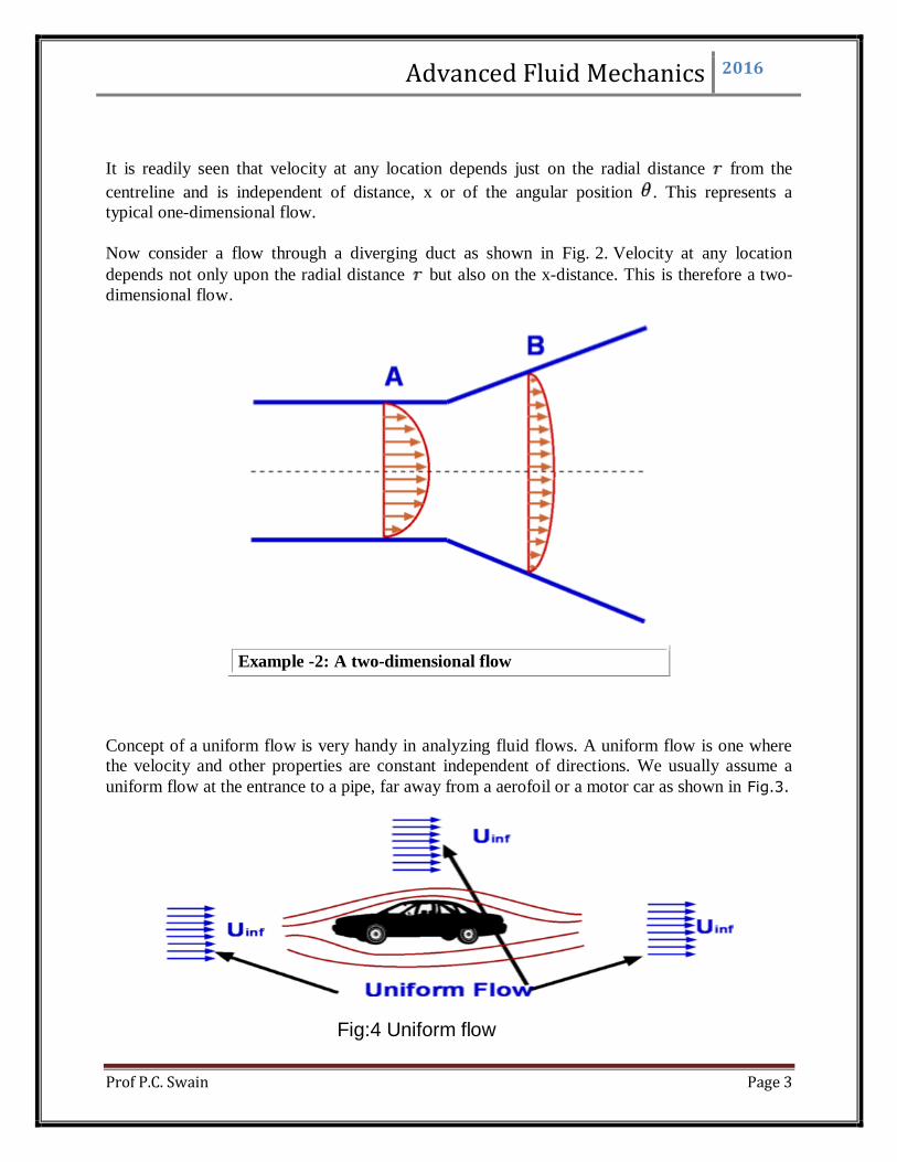
Now consider a flow through a diverging duct as shown in Fig. 2. Velocity at any location
depends not only upon the radial distance but also on the x-distance. This is therefore a two-
dimensional flow.
Example -2: A two-dimensional flow
Concept of a uniform flow is very handy in analyzing fluid flows. A uniform flow is one where
the velocity and other properties are constant independent of directions. We usually assume a
uniform flow at the entrance to a pipe, far away from a aerofoil or a motor car as shown in Fig.3.
Fig:4 Uniform flow

Advanced Fluid Mechanics 2016
Prof P.C. Swain Page 4
1. Real fluids
The flow of real fluids exhibits viscous effect that is they tend to "stick" to solid surfaces and
have stresses within their body.
You might remember from earlier in the course Newton’s law of viscosity:
This tells us that the shear stress, 𝜏in a fluid is proportional to the velocity gradient - the rate of
change of velocity across the fluid path. For a "Newtonian" fluid we can write:
Where the constant of proportionality, 𝜇 is known as the coefficient of viscosity (or simply
viscosity). We saw that for some fluids - sometimes known as exotic fluids - the value
of 𝜇 changes with stress or velocity gradient. We shall only deal with Newtonian fluids.
In his lecture we shall look at how the forces due to momentum changes on the fluid and viscous
forces compare and what changes take place.
2.Laminar and turbulent flow
If we were to take a pipe of free flowing water and inject a dye into the middle of the stream,
what would we expect to happen?
This
Advanced Fluid Mechanics 2016
Prof P.C. Swain Page 5
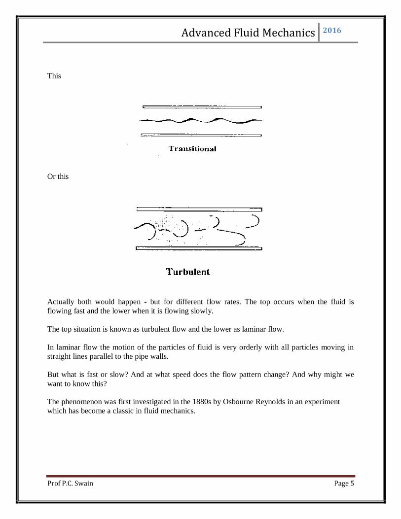
This
Or this
Actually both would happen - but for different flow rates. The top occurs when the fluid is
flowing fast and the lower when it is flowing slowly.
The top situation is known as turbulent flow and the lower as laminar flow.
In laminar flow the motion of the particles of fluid is very orderly with all particles moving in
straight lines parallel to the pipe walls.
But what is fast or slow? And at what speed does the flow pattern change? And why might we
want to know this?
The phenomenon was first investigated in the 1880s by Osbourne Reynolds in an experiment
which has become a classic in fluid mechanics.

Advanced Fluid Mechanics 2016
Prof P.C. Swain Page 6
He used a tank arranged as above with a pipe taking water from the centre into which he injected
a dye through a needle. After many experiments he saw that this expression
where 𝜌 = density, u = mean velocity, d = diameter and 𝑣 = viscosity
would help predict the change in flow type. If the value is less than about 2000 then flow is
laminar, if greater than 4000 then turbulent and in between these then in the transition zone.
This value is known as the Reynolds number, Re:
Laminar flow: Re < 2000
Transitional flow: 2000 < Re < 4000
Turbulent flow: Re > 4000
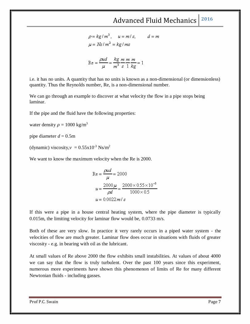
What are the units of this Reynolds number? We can fill in the equation with SI units:
Advanced Fluid Mechanics 2016
Prof P.C. Swain Page 7
i.e. it has no units. A quantity that has no units is known as a non-dimensional (or dimensionless)
quantity. Thus the Reynolds number, Re, is a non-dimensional number.
We can go through an example to discover at what velocity the flow in a pipe stops being
laminar.
If the pipe and the fluid have the following properties:
water density 𝜌 = 1000 kg/m3
pipe diameter d = 0.5m
(dynamic) viscosity,ν = 0.55x10⁻³ Ns/m2
We want to know the maximum velocity when the Re is 2000.
If this were a pipe in a house central heating system, where the pipe diameter is typically
0.015m, the limiting velocity for laminar flow would be, 0.0733 m/s.
Both of these are very slow. In practice it very rarely occurs in a piped water system - the
velocities of flow are much greater. Laminar flow does occur in situations with fluids of greater
viscosity - e.g. in bearing with oil as the lubricant.
At small values of Re above 2000 the flow exhibits small instabilities. At values of about 4000
we can say that the flow is truly turbulent. Over the past 100 years since this experiment,
numerous more experiments have shown this phenomenon of limits of Re for many different
Newtonian fluids - including gasses.

Advanced Fluid Mechanics 2016
Prof P.C. Swain Page 8
What does this abstract number mean?
We can say that the number has a physical meaning, by doing so it helps to understand some of
the reasons for the changes from laminar to turbulent flow.
It can be interpreted that when the inertial forces dominate over the viscous forces (when the
fluid is flowing faster and Re is larger) then the flow is turbulent. When the viscous forces are
dominant (slow flow, low Re) they are sufficient enough to keep all the fluid particles in line,
then the flow is laminar.
Laminar flow
Re < 2000
'low' velocity
Dye does not mix with water
Fluid particles move in straight lines
Simple mathematical analysis possible
Rare in practice in water systems.
Transitional flow
2000 > Re < 4000
'medium' velocity
Dye stream wavers in water - mixes slightly.
Turbulent flow
Re > 4000
'high' velocity
Dye mixes rapidly and completely
Particle paths completely irregular
Average motion is in the direction of the flow
Cannot be seen by the naked eye
Changes/fluctuations are very difficult to detect. Must use laser.
Mathematical analysis very difficult - so experimental measures are used

Advanced Fluid Mechanics 2016
Prof P.C. Swain Page 9
3. Pressure loss due to friction in a pipeline
Up to this point on the course we have considered ideal fluids where there have been no losses
due to friction or any other factors. In reality, because fluids are viscous, energy is lost by
flowing fluids due to friction which must be taken into account. The effect of the friction shows
itself as a pressure (or head) loss.
In a pipe with a real fluid flowing, at the wall there is a shearing stress retarding the flow, as
shown below.
If a manometer is attached as the pressure (head) difference due to the energy lost by the fluid
overcoming the shear stress can be easily seen.
The pressure at 1 (upstream) is higher than the pressure at 2.
We can do some analysis to express this loss in pressure in terms of the forces acting on the
fluid.
Advanced Fluid Mechanics 2016
Prof P.C. Swain Page 10
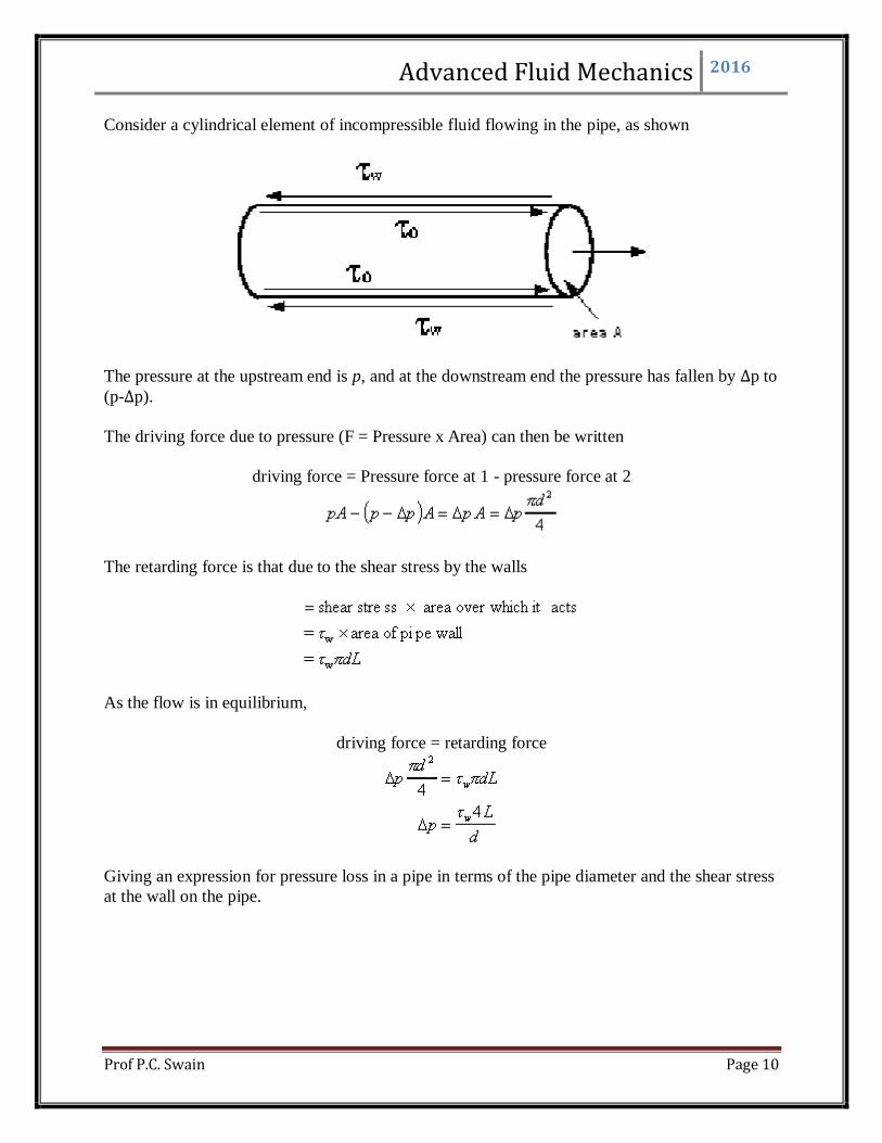
Consider a cylindrical element of incompressible fluid flowing in the pipe, as shown
The pressure at the upstream end is p, and at the downstream end the pressure has fallen by ∆p to
(p-∆p).
The driving force due to pressure (F = Pressure x Area) can then be written
driving force = Pressure force at 1 - pressure force at 2
The retarding force is that due to the shear stress by the walls
As the flow is in equilibrium,
driving force = retarding force
Giving an expression for pressure loss in a pipe in terms of the pipe diameter and the shear stress
at the wall on the pipe.

Advanced Fluid Mechanics 2016
Prof P.C. Swain Page 11
The shear stress will vary with velocity of flow and hence with Re. Many experiments have been
done with various fluids measuring the pressure loss at various Reynolds numbers. These results
plotted to show a graph of the relationship between pressure loss and Re look similar to the
figure below:
This graph shows that the relationship between pressure loss and Re can be expressed as
As these are empirical relationships, they help in determining the pressure loss but not in finding
the magnitude of the shear stress at the wall on a particular fluid. We could then use it to give a
general equation to predict the pressure loss.
Advanced Fluid Mechanics 2016
Prof P.C. Swain Page 12
4. Pressure loss during laminar flow in a pipe
In general the shear stress w. is almost impossible to measure. But for laminar flow it is possible
to calculate a theoretical value for a given velocity, fluid and pipe dimension.
In laminar flow the paths of individual particles of fluid do not cross, so the flow may be
considered as a series of concentric cylinders sliding over each other - rather like the cylinders of
a collapsible pocket telescope.
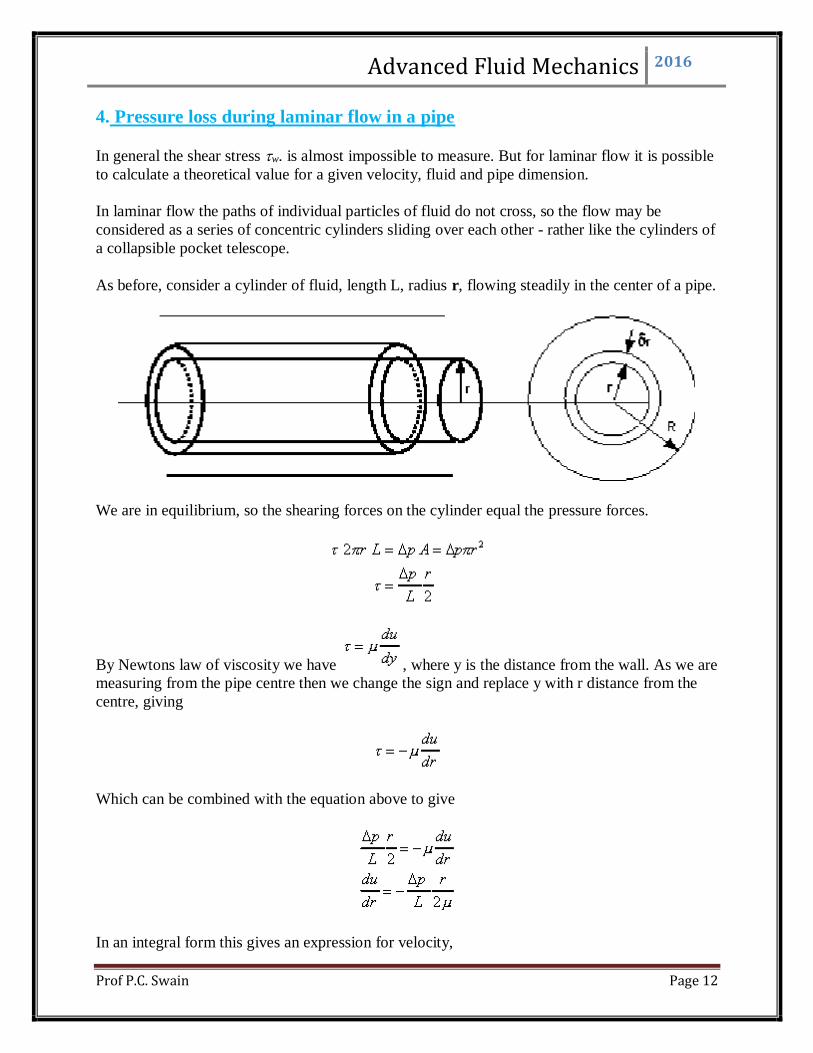
As before, consider a cylinder of fluid, length L, radius r, flowing steadily in the center of a pipe.
We are in equilibrium, so the shearing forces on the cylinder equal the pressure forces.
By Newtons law of viscosity we have , where y is the distance from the wall. As we are
measuring from the pipe centre then we change the sign and replace y with r distance from the
centre, giving
Which can be combined with the equation above to give
In an integral form this gives an expression for velocity,

Advanced Fluid Mechanics 2016
Prof P.C. Swain Page 13
Integrating gives the value of velocity at a point distance r from the centre
At r = 0, (the centre of the pipe), u = umax, at r = R (the pipe wall) u = 0, giving
so, an expression for velocity at a point r from the pipe centre when the flow is laminar is
Note how this is a parabolic profile (of the form y = ax2 + b ) so the velocity profile in the pipe
looks similar to the figure below
Advanced Fluid Mechanics 2016
Prof P.C. Swain Page 14
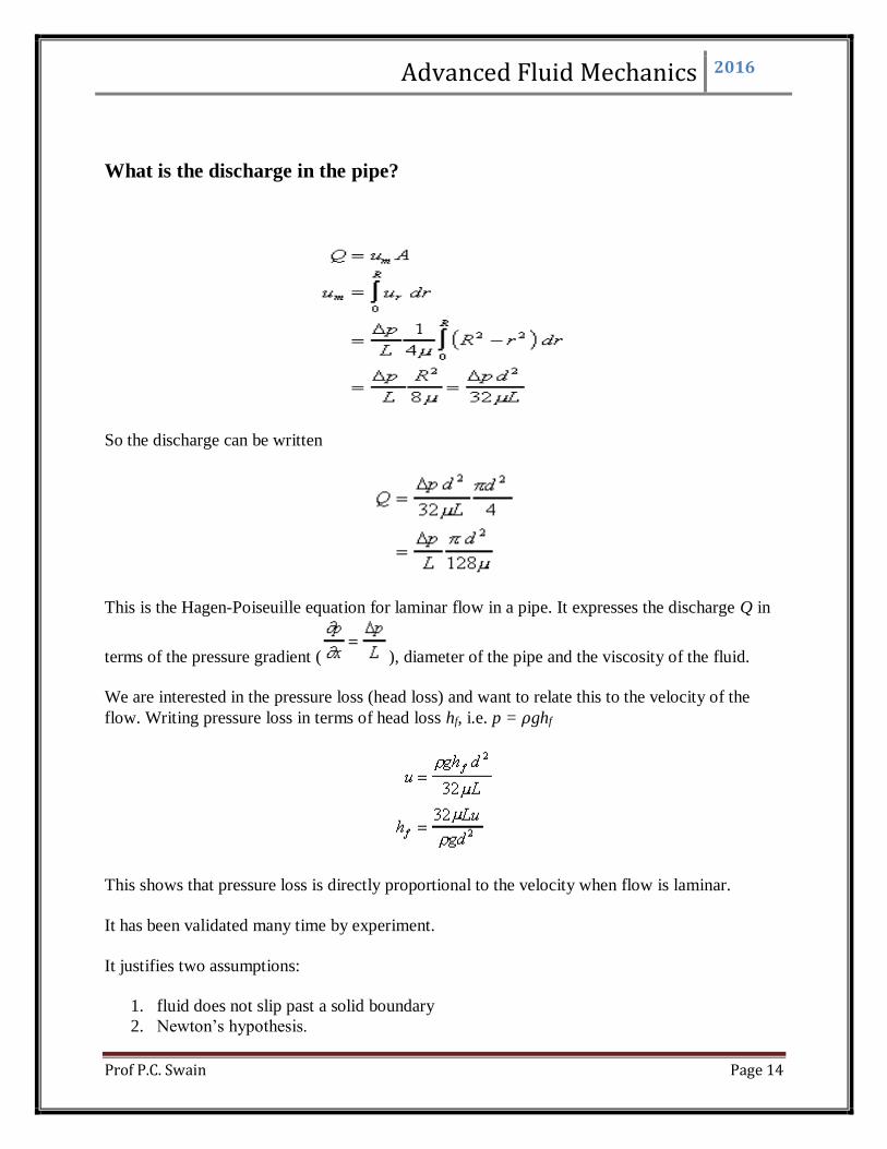
What is the discharge in the pipe?
So the discharge can be written
This is the Hagen-Poiseuille equation for laminar flow in a pipe. It expresses the discharge Q in
terms of the pressure gradient ( ), diameter of the pipe and the viscosity of the fluid.
We are interested in the pressure loss (head loss) and want to relate this to the velocity of the
flow. Writing pressure loss in terms of head loss hf, i.e. p = 𝜌ghf
This shows that pressure loss is directly proportional to the velocity when flow is laminar.
It has been validated many time by experiment.
It justifies two assumptions:
1. fluid does not slip past a solid boundary
2. Newton’s hypothesis.

Advanced Fluid Mechanics 2016
Prof P.C. Swain Page 15
Streamline :
This is an imaginary curve in a flow field for a fixed instant of time, tangent to which gives
the instantaneous velocity at that point . Two stream lines can never intersect each
other, as the instantaneous velocity vector at any given point is unique.
The differential equation of streamline may be written as
𝑑𝑢
𝑢=
𝑑𝑣
𝑣=
𝑑𝑤
𝑤
whereu,v, and w are the velocity components in x, y and z directions respectively
as sketched.
Fig. Streamlines
Fig. Streamline function

Advanced Fluid Mechanics 2016
Prof P.C. Swain Page 16
Stream tube :
If streamlines are drawn through a closed curve, they form a boundary surface across which fluid
cannot penetrate. Such a surface bounded by streamlines is a sort of tube, and is known as a
streamtube.
From the definitionof streamline, it is evident that no fluid can cross the bounding surface of the
streamtube. This implies that the quantity(mass) of fluid entering the streamtube at one end must
be the same as the quantity leaving it at the other. The streamtubeis generally assumed to be a
small cross-sectional area so that the velocity over it could be considered uniform.
Fig.Streamtube
Pathline :
A pathline is the locus of a fluid particle as it moves along. In others word, a pathline is a curve
traced by a single fluid particle during its motion.
Two path lines can intersect each other as or a single path line can form a loop as different
particles or even same particle can arrive at the same point at different instants of time.
Fig.Pathline
Advanced Fluid Mechanics 2016
Prof P.C. Swain Page 17
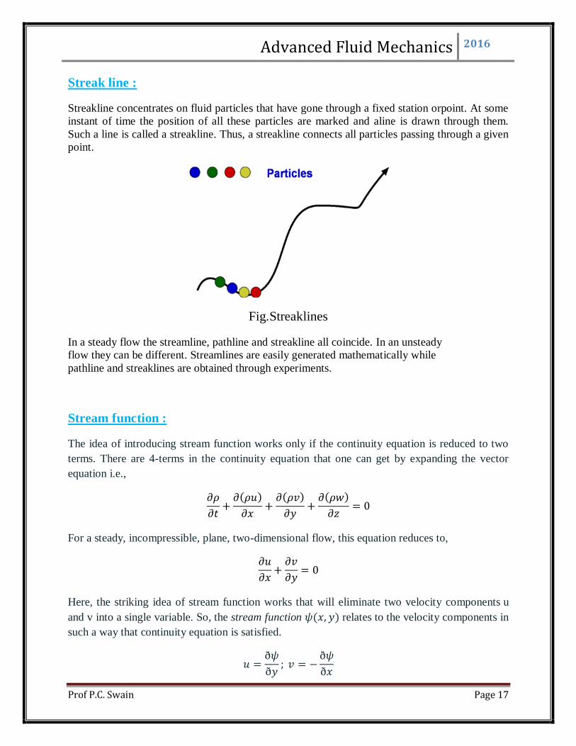
Streak line :
Streakline concentrates on fluid particles that have gone through a fixed station orpoint. At some
instant of time the position of all these particles are marked and aline is drawn through them.
Such a line is called a streakline. Thus, a streakline connects all particles passing through a given
point.
Fig.Streaklines
In a steady flow the streamline, pathline and streakline all coincide. In an unsteady
flow they can be different. Streamlines are easily generated mathematically while
pathline and streaklines are obtained through experiments.
Stream function :
The idea of introducing stream function works only if the continuity equation is reduced to two
terms. There are 4-terms in the continuity equation that one can get by expanding the vector
equation i.e.,
𝜕𝜌
𝜕𝑡+
𝜕(𝜌𝑢)
𝜕𝑥+
𝜕(𝜌𝑣)
𝜕𝑦+
𝜕(𝜌𝑤)
𝜕𝑧= 0
For a steady, incompressible, plane, two-dimensional flow, this equation reduces to,
𝜕𝑢
𝜕𝑥+
𝜕𝑣
𝜕𝑦= 0
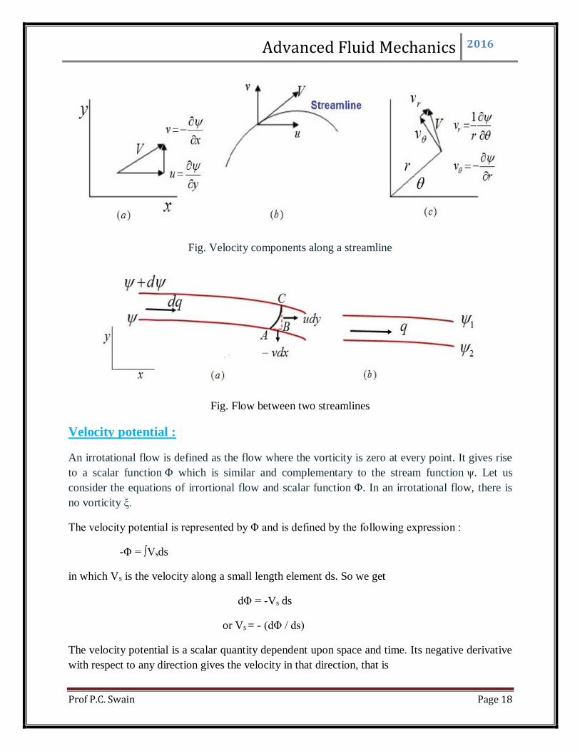
Here, the striking idea of stream function works that will eliminate two velocity components u
and v into a single variable. So, the stream function 𝜓(𝑥, 𝑦) relates to the velocity components in
such a way that continuity equation is satisfied.
𝑢 =ð𝜓
ð𝑦; 𝑣 = −
ð𝜓
ð𝑥
Advanced Fluid Mechanics 2016
Prof P.C. Swain Page 18
Fig. Velocity components along a streamline
Fig. Flow between two streamlines
Velocity potential :
An irrotational flow is defined as the flow where the vorticity is zero at every point. It gives rise
to a scalar function Φ which is similar and complementary to the stream function ψ. Let us
consider the equations of irrortional flow and scalar function Φ. In an irrotational flow, there is
no vorticity ξ.
The velocity potential is represented by Φ and is defined by the following expression :
-Φ = ∫Vsds
in which Vs is the velocity along a small length element ds. So we get
dΦ = -Vs ds
or Vs = - (dΦ / ds)
The velocity potential is a scalar quantity dependent upon space and time. Its negative derivative
with respect to any direction gives the velocity in that direction, that is

Advanced Fluid Mechanics 2016
Prof P.C. Swain Page 19
𝑢 = −𝜕Φ
𝜕𝑥 , 𝑣 = −
𝜕Φ
𝜕𝑦 , 𝑤 = −
𝜕Φ
𝜕𝑧
In polar co-ordinates (r, θ, z), the velocity components are
vr= − 𝜕Φ
𝜕𝑟 , vθ =
𝜕Φ
𝑟 𝜕𝑟 , vz = −
𝜕Φ
𝜕𝑧
The velocity potential Φ thus provides an alternative means of expressing velocity components.
The minus sign in equation appears because of the convention that the velocity potential
decreases in the direction of flow just as the electrical potential decreases in the direction in
which the current flows. The velocity potential is not a physical quantity which could be directly
measured and, therefore, its zero position may be arbitrarily chosen.
Flownet :
The flownet is a graphical representation of two-dimensional irrotational flow and consists of a
family of streamlines intersecting orthogonally a family of equipotential lines (they intersect at
right angles) and in the process forming small curvilinear squares.
Fig.Flownet
Uses of flownet :
For given boundaries of flow, the velocity and pressure distribution can be determined, if
the velocity distribution and pressure at any reference section are known
Loss of flow due to seepage in earth dams and unlined canals can be evaluated
Uplift pressures on the undesirable (bottom) of the dam can be worked out
Relation between stream function & velocity potential

Advanced Fluid Mechanics 2016
Prof P.C. Swain Page 20
∅exists only in irrotational flow where as 𝜑exists in both rotational as well as irrotational
flow
u= -𝜕∅
𝜕𝑥=
𝜕𝜑
𝜕𝑦& v=
𝜕𝜑
𝜕𝑥 = -
𝜕∅
𝜕𝑦
therefore, 𝜕𝜑
𝜕𝑥 =
𝜕∅
𝜕𝑦&
𝜕∅
𝜕𝑥= −
𝜕𝜑
𝜕𝑦
Advanced Fluid Mechanics 2016
Prof P.C.Swain Page 1
Lecture Note 3
Potential Flow
Introduction
In a plane irrotaional flow, one can use either velocity potential or stream function to define the
flow field and both must satisfy Laplace equation . Moreover, the analysis of this equation is
much easier than direct approach of fully viscous Navier-Stokes equations. Since
the Laplace equation is linear, various solutions can be added to obtain other solutions. Thus, if
we have certain basic solutions, then they can be combined to obtain complicated and interesting
solutions. The analysis of such flow field solutions of Laplace equation is termed as potential
theory . The potential theory has a lot of practical implications defining complicated flows. Here,
we shall discuss the stream function and velocity potential for few elementary flow fields such as
uniform flow, source/sink flow and vortex flow. Subsequently, they can be superimposed to
obtain complicated flow fields of practical relevance.
Governing equations for irrotational and incompressible flow
The analysis of potential flow is dealt with combination of potential lines and streamlines. In
a planner flow, the velocities of the flow field can be defined in terms of stream
functions and potential functions as,
(3.4.1)
The stream function is defined such that continuity equation is satisfied whereas, for low
speed irrotational flows , if the viscous effects are neglected, the continuity
equation , reduces to Laplace equation for . Both the functions satisfy the Laplace equations i.e.
(3.4.3)
Thus, the following obvious and important conclusions can be drawn from Eq. (3.4.2);

Advanced Fluid Mechanics 2016
Prof P.C.Swain Page 2
• Any irrotational, incompressible and planner flow (two-dimensional) has a velocity potential and stream function and both the functions satisfy Laplace equation.
• Conversely, any solution of Laplace equation represents the velocity potential or stream function for an irrotational, incompressible and two-dimensional flow.
Note that Eq. (3.4.2) is a second-order linear partial differential equation. If there
are n separate solutions such as, then the sum (Eq. 3.4.3) is
also a solution of Eq. (3.4.2).
(3.4.3)
It leads to an important conclusion that a complicated flow pattern for an irrotational,
incompressible flow can be synthesized by adding together a number of elementary flows
which are also irrotational and incompressible. However, different values of
represent the different streamline patterns of the body and at the same time they satisfy the Laplace equation. In order to differentiate the streamline patterns of different bodies, it
is necessary to impose suitable boundary conditions as shown in Fig. 3.4.1. The most
common boundary conditions include far-field and wall boundary conditions. on the surface of the body (i.e. wall).
Fig. 3.4.1: Boundary conditions of a streamline body.
Far away from the body, the flow approaches uniform free stream conditions in all
directions. The velocity field is then specified in terms of stream function and potential function as,

Advanced Fluid Mechanics 2016
Prof P.C.Swain Page 3
(3.4.4)
On the solid surface, there is no velocity normal to the body surface while the tangent at
any point on the surface defines the surface velocity. So, the boundary conditions can be written in terms of stream and potential functions as,
(3.4.5)
Here, s is the distance measured along the body surface and n is perpendicular to the body.
Thus, any line of constant in the flow may be interpreted as body shape for which there
is no velocity normal to the surface. If the shape of the body is given by ,
then is alternate boundary condition of Eq. (3.4.5). If we deal with
wall boundary conditions in terms of , then the equation of streamline evaluated at body surface is given by,
(3.4.6)
It is seen that lines of constant (equi-potential lines) are orthogonal to lines of
constant (streamlines) at all points where they intersect. Thus, for a potential flow field, a flow-net consisting of family of streamlines and potential lines can be drawn, which are
orthogonal to each other. Both the set of lines are laplacian and they are useful tools to visualize the flow field graphically.
Referring to the above discussion, the general approach to the solution of irrotational, incompressible flows can be summarized as follows;
• Solve the Laplace equation for along with proper boundary conditions.
• Obtain the flow velocity from Eq. (3.4.1)
• Obtain the pressure on the surface of the body using Bernoulli's equation.
(3.4.7)
Advanced Fluid Mechanics 2016
Prof P.C.Swain Page 4
In the subsequent section, the above solution procedure will be applied to some basic
elementary incompressible flows and later they will be superimposed to synthesize more complex flow problems.
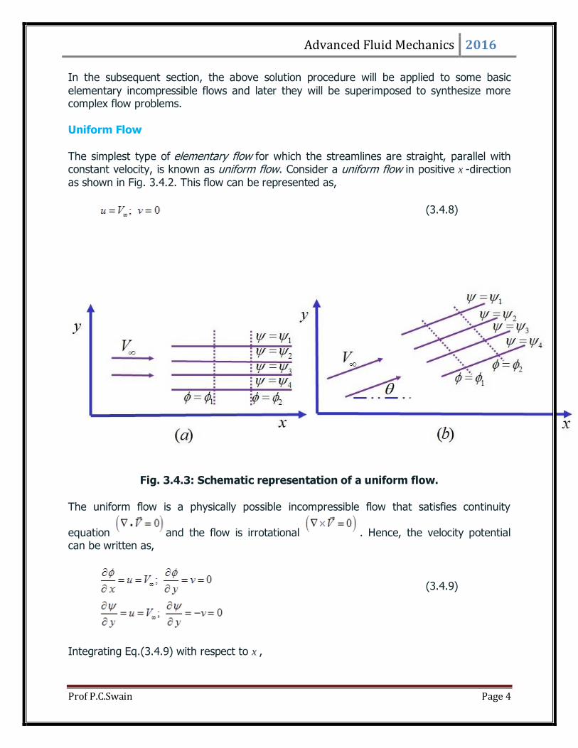
Uniform Flow
The simplest type of elementary flow for which the streamlines are straight, parallel with constant velocity, is known as uniform flow. Consider a uniform flow in positive x -direction
as shown in Fig. 3.4.2. This flow can be represented as,
(3.4.8)
Fig. 3.4.3: Schematic representation of a uniform flow.
The uniform flow is a physically possible incompressible flow that satisfies continuity
equation and the flow is irrotational . Hence, the velocity potential can be written as,
(3.4.9)
Integrating Eq.(3.4.9) with respect to x ,
Advanced Fluid Mechanics 2016
Prof P.C.Swain Page 5
(3.4.10)
In practical flow problems, the actual values of are not important, rather it is
always used as differentiation to obtain the velocity vector. Hence, the constant appearing in Eq. (3.4.10) can be set to zero. Thus, for a uniform flow, the stream functions and potential function can be written as,
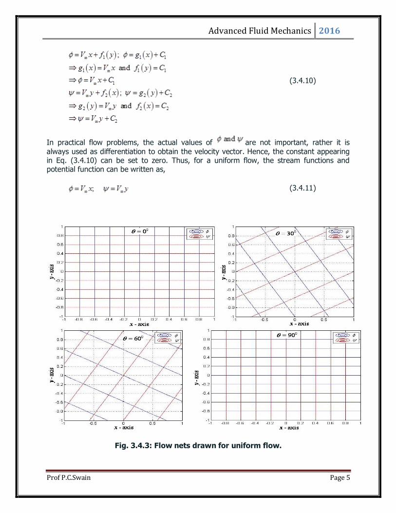
(3.4.11)
Fig. 3.4.3: Flow nets drawn for uniform flow.

Advanced Fluid Mechanics 2016
Prof P.C.Swain Page 6
When Eq. (3.4.11), is substituted in Eq. (3.4.3), Laplace equation is satisfied. Further, if the uniform flow is at an angle θ with respect to x -axis as shown in Fig. 3.4.3, then the
generalized form of stream function and potential function is represented as follows;
(3.4.13)
The flow nets can be constructed by assuming different values of constants in Eq. (3.4.11) and with different angle θ as shown in Fig. 3.4.3. The circulation in a uniform flow along a
closed curve is zero which gives the justification that the uniform flow is irrotational in nature.
(3.4.13)
Source/Sink Flow
Consider a two-dimensional incompressible flow where the streamlines are radially outward from a central point ‘O' (Fig. 3.4.4). The velocity of each streamlines varies inversely with
the distance from point ‘O'. Such a flow is known as source flow and its opposite case is the sink flow , where the streamlines are directed towards origin. Both the source and
sink flow are purely radial. Referring to the Fig. 3.4.4, if are the components of
velocities along radial and tangential direction respectively, then the equations of the
streamlines that satisfy the continuity equation are,
(3.4.14)
Here, the constant c can be related to the volume flow rate of the source. If we define
as the volume flow rate per unit length perpendicular to the plane, then,
(3.4.15)
The potential function can be obtained by writing the velocity field in terms of cylindrical
coordinates. They may be written as,

Advanced Fluid Mechanics 2016
Prof P.C.Swain Page 7
(3.4.16)
Fig. 3.4.4: Schematic representation of a source and sink flow.
Integrating Eq. (3.4.16) with respect to , we can get the equation for potential function and stream function for a source and sink flow.
(3.4.17)
The constant appearing in Eqs (3.4.17) can be dropped to obtain the stream function and
potential function.
Advanced Fluid Mechanics 2016
Prof P.C.Swain Page 8
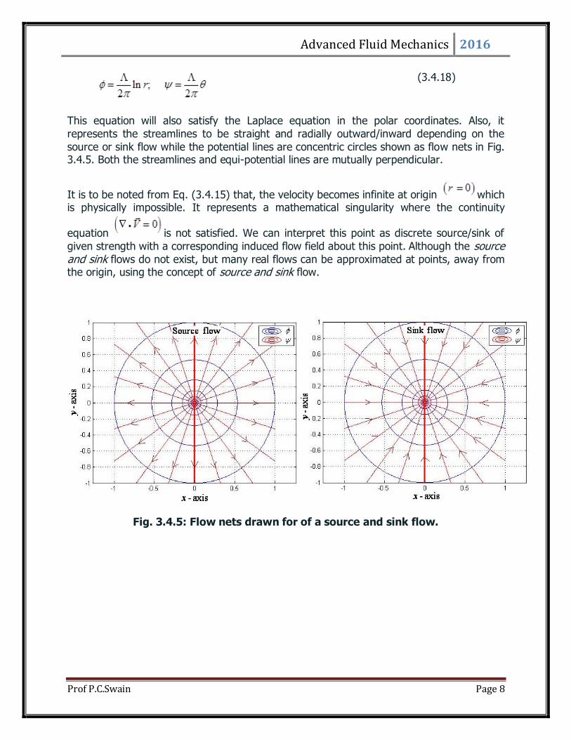
(3.4.18)
This equation will also satisfy the Laplace equation in the polar coordinates. Also, it
represents the streamlines to be straight and radially outward/inward depending on the
source or sink flow while the potential lines are concentric circles shown as flow nets in Fig. 3.4.5. Both the streamlines and equi-potential lines are mutually perpendicular.
It is to be noted from Eq. (3.4.15) that, the velocity becomes infinite at origin which is physically impossible. It represents a mathematical singularity where the continuity
equation is not satisfied. We can interpret this point as discrete source/sink of
given strength with a corresponding induced flow field about this point. Although the source and sink flows do not exist, but many real flows can be approximated at points, away from the origin, using the concept of source and sink flow.
Fig. 3.4.5: Flow nets drawn for of a source and sink flow.

Advanced Fluid Mechanics 2016
Prof P.C.Swain
References:
1. Wand D.J., and Harleman D.R. (91964) “Fluid Dynamics”, Addison Wesley.
2. Schlichting, H.: (1976) “Boundary Layer theory”, International Text –
Butterworth
3. Lamb, H. (1945) “Hydrodynamics”, International Text – Butterworth
4. Lamb, H.R. (1945) “Hydrodynamics”, Rover Publications
5. Rouse, H. (1957), “Advanced Fluid Mechanics”, John Wiley & Sons, N
York
6. White, F.M. (1980) “Viscous Fluid Flow”, McGraw Hill Pub. Co, N York
7. Yalin, M.S.(1971), “Theory of Hydraulic Models”, McMillan Co., 1971.
8. Mohanty A.K. (1994), “Fluid Mechanics”, Prentice Hall of India, N Delhi
Related Documents