MC3D Premixing Analysis using X-Ray Radioscopy ... Paper - MC3D... · MC3D Premixing Analysis using X-Ray ... The 8th European Review Meeting on Severe Accident Research ... smaller

*Corresponding author

Email address: [email protected] (M.Leskovar)

MC3D Premixing Analysis using X-Ray Radioscopy Experimental

Data of KROTOS-SERENA Tests

M.Leskovara*, V.Centriha, M.Uršiča, N.Cassiaut Louisb, C.Brayerb, P.Pilusob

a Jožef Stefan Institute, Jamova cesta 39, 1000 Ljubljana, Slovenia b CEA Cadarache, 13108 Saint Paul lez Durance CEDEX, France

Abstract

A steam explosion is an energetic Fuel-Coolant Interaction process, which may occur during a severe

reactor accident when the molten core comes into contact with the coolant water. An important condition for the

occurrence of an energetic steam explosion is the nature of the initial coarse premixing of the melt and water.

The most distinctive process for the premixture formation is the melt jet fragmentation during the penetration

into water. Various experimental and analytical activities were carried out in the frame of the recent OECD

SERENA-Phase 2 project to better understand and model reliably the process of the premixing phase. The

comprehensive analysis of the X-ray radioscopy data for the KROTOS-SERENA tests was completed at CEA-

Cadarache. The analysis of the post-processed X-ray images provides an important insight into the complex

premixing process. The new information about the melt jet release and the premixture formation provided by the

innovative X-ray radioscopy system was used in the performed premixing analysis with the MC3D computer

code developed by IRSN. MC3D is a multi-dimensional Eulerian code devoted to study multi-phase and multi-

constituent flows in the field of nuclear safety.

Because the local data of the premixed region may be obtained from the X-ray images, the performed study

is focused mainly on the lateral distribution of the premixture along the KROTOS test section. Based on the melt

jet mass flow rate and the melt jet-water impact velocity, deduced from the X-ray radioscopy data, an

appropriate MC3D model of the melt release system was developed first. By comparison of the premixing

simulation results with the experimental data the “best estimate” model parameters were established. Then, the

influence of the water sub-cooling and the corium composition on the lateral distributions of the void and melt

droplets were analysed. Finally, a parametric analysis was performed, varying the most important MC3D jet

breakup model parameters: melt jet fragmentation rate, Sauter diameter and radial velocity of generated melt

droplets, and turbulent diffusion coefficient of melt droplets. In the paper, the results obtained with MC3D

calculations are discussed and compared to the experimental one from the KROTOS tests.

Keywords: Fuel-coolant interaction, Premixing, Jet breakup, Radioscopy

1. Introduction

During a hypothetical severe accident in a pressurized water reactor the molten core may be released from

the failed reactor vessel into the flooded reactor cavity. The resulting Fuel-Coolant Interaction (FCI) may lead to

an energetic Steam Explosion (SE). An important condition for the occurrence of a steam explosion is the nature

of the initial coarse premixing of the melt and water, where the most distinctive part of the premixture formation

is the melt jet fragmentation during the penetration into water. The SE occurs when due to melt fine

fragmentation feedback mechanisms, the heat transfer between the melt and the water becomes so rapid that the

heat transfer time scale becomes shorter than the pressure relief time scale [1]. It represents an important nuclear

safety issue because a strong enough SE in a nuclear power plant could potentially damage directly or indirectly

the containment integrity and thus lead to the radioactive release into the environment [2], [3]. Various

experimental and analytical activities were carried out in the frame of the recent OECD SERENA-Phase 2

project to better understand the FCI phenomena and model reliably the process of the premixing phase [4]. The

comprehensive analysis of the X-ray radioscopy data for the KROTOS-SERENA (KS) experiments was

completed at CEA-Cadarache [5]. Figure 1 shows the KROTOS test facility and the position of the radioscopy

window along the test tube in different KROTOS experimental tests (KFC and KS-1 to KS-6). In the KROTOS

KS tests series, the test tube is filled with water usually up to 1.145 m. Approximately 200 x 300 mm radioscopy

image frame covers fully the test tube diameter of 0.2 m. The highest position of the image frame was in the

KS-1 test (1.0 to 1.3 m) and the lowest in the KS-2 test (0.55 to 0.85 m) [5]. In tests KS-4 to KS-6 the position of

the X-ray image was the same.

mailto:[email protected]

The 8th European Review Meeting on Severe Accident Research - ERMSAR-2017

Warsaw, Poland, 16-18 May 2017

SESSION: Ex-vessel corium interactions and coolability, Paper N° 207

Characterization of the premixing evolution is based on two basic components, the molten corium (melt jet

and melt droplets) and the void fraction (produced vapour). In the experiments, the melt propagation is initially

followed by sacrificial thermocouples (ZT’s) readings placed vertically along the test tube. The global void

fraction under the water level is generally deduced from the water level transducer. Radioscopy data provide

various additional information regarding the corium melt jet, its fragmentation and the void fraction formation.

Several qualitative and quantitative data for corium and void were post processed with developed various

innovative X-ray image processing techniques and analysis algorithms [5], [6], [7]. The presented study relies

mainly on the cumulative evolution of the corium volume passing through the X-ray image and on the evolution

of the void volume and fraction within the X-ray image as well as the void volume distribution at the moment

preceding the SE triggering. Based on the cumulative corium evolution the melt mass flow rate may be

fine-tuned in the modelling. The jet impact velocity and the jet fragmentation length may be revisited from X-ray

images. The local data of the void volume distribution at the triggering time may provide the information about

the influence of some important experimental conditions. Namely, it was observed that the sub-cooling

conditions might have some influence on the lateral premixture extension [5].

Figure 1 KROTOS facility with test tube filled with water (left) and schematic visualisation of the X-ray window (image)

position in different KROTOS tests [5] (right). Image positions are compared relatively to the water level in each test.

Within the broader aim to improve the understanding of the premixing, the objective of the presented study

is to take advantage of the post-processed radioscopy data [5] and improve the premixing phase modelling. First,

the X-ray observations are overviewed and an appropriate MC3D model of the melt release system is

established. Based on the X-ray data, the melt jet release modelling with MC3D is improved by focusing on the

melt mass flow rate, the jet impact velocity and the jet fragmentation length. Second, the simulation of the

premixing phase is performed and compared to the experimental results. To compare the lateral void distribution

at the triggering time, a quantitative indicator of the lateral premixture extension was set up. In the end, the

analysis method is evaluated and parametric simulations are performed. The void and the melt droplets

distributions are both analysed. The parametric analysis focuses on the influence of the experimental conditions

(water sub-cooling and material composition) and the specific modelling parameters (melt jet fragmentation rate,

Sauter diameter and radial velocity of generated melt droplets, and turbulent diffusion coefficient of melt

droplets) on the lateral premixture extension. The simulations were performed with the MC3D computer code,

which is being developed by IRSN, France [8], [9].

2. Experimental Observations and Modelling Conditions

2.1. KROTOS KS X-Ray Data

The most relevant X-ray data for corium were obtained from the KFC and KS-1 tests, because the X-ray

window was positioned near or a bit above the water level (Figure 1), where the premixing is not so complex.

Because of the significant fragmentation in the lower test tube area the X-ray images for other experimental tests

were too complex to provide reliable corium mass results [5]. However, for determining the factors, such as the

mass flow rate and the jet impact velocity, the data near the water level are the most useful. Figure 2 reviews the

estimated corium mass evolution, i.e. the cumulative delivered mass, the mass within the X-ray window frame

and the mass below the window for the first two tests, KFC (left) and KS-1 (right). Due to similar experimental

KFC KS-1 KS-2 KS-4

Water level

Water depth

0.00 m

0.15 m

0.30 m

0.45 m

0.60 m

KS-5

KS-6

Water: 1145 mm

The 8th European Review Meeting on Severe Accident Research -ERMSAR-2017



conditions and similar X-ray window position, the corium data from KFC and KS-1 in Figure 2 may be

compared to some extent. The radioscopy image analysis has been performed in the area below the initial water

level [5]. The starting point in the diagrams in Figure 2 is the arrival of the melt jet in the water. Each test’s data

ends at the triggering time. The slope of the cumulative delivered corium (Total) represents the mass flow rate of

the delivered melt in the water. One important difference between the KFC and KS-1 melt releases is the use of a

“fusible” disc, which was used in KS-1 and allowed to have the melt at zero velocity at this level and ensured the

gravity melt pouring in the form of a coherent jet [5]. Due to the non-suspended type of melt release, a bit more

complex melt release may be observed in the KFC test, starting with the smaller amount of faster initial melt

spray for the first 0.3 s. By comparing the corium mass within the X-ray window (InFrame) it may be observed,

that after the initial droplet spray in KFC (from 0.3 s further) a bit more mass is present within the image in KFC

compared to KS-1. This should be first attributed to the fact that the area of the analysed X-ray image in KS-1 is

smaller than in KFC due to the position of the X-ray frame and the fact that the area above the water level is

neglected, Figure 1.

Figure 2 Comparison of corium mass evolution for KFC (left) and KS-1 (right) tests [5]: estimated cumulative mass delivered

into water (Total), mass within X-ray image (InFrame) and estimated mass below the X-ray window (Below).

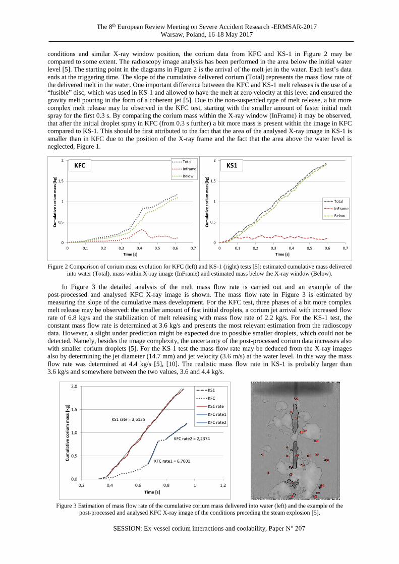
In Figure 3 the detailed analysis of the melt mass flow rate is carried out and an example of the

post-processed and analysed KFC X-ray image is shown. The mass flow rate in Figure 3 is estimated by

measuring the slope of the cumulative mass development. For the KFC test, three phases of a bit more complex

melt release may be observed: the smaller amount of fast initial droplets, a corium jet arrival with increased flow

rate of 6.8 kg/s and the stabilization of melt releasing with mass flow rate of 2.2 kg/s. For the KS-1 test, the

constant mass flow rate is determined at 3.6 kg/s and presents the most relevant estimation from the radioscopy

data. However, a slight under prediction might be expected due to possible smaller droplets, which could not be

detected. Namely, besides the image complexity, the uncertainty of the post-processed corium data increases also

with smaller corium droplets [5]. For the KS-1 test the mass flow rate may be deduced from the X-ray images

also by determining the jet diameter (14.7 mm) and jet velocity (3.6 m/s) at the water level. In this way the mass

flow rate was determined at 4.4 kg/s [5], [10]. The realistic mass flow rate in KS-1 is probably larger than

3.6 kg/s and somewhere between the two values, 3.6 and 4.4 kg/s.

Figure 3 Estimation of mass flow rate of the cumulative corium mass delivered into water (left) and the example of the

post-processed and analysed KFC X-ray image of the conditions preceding the steam explosion [5].

0

0,5

1

1,5

2

0 0,1 0,2 0,3 0,4 0,5 0,6 0,7

Cum

ula

tive

co

riu

m m

ass

[kg

]

Time [s]

Total

Inframe

Below

KFC

0

0,5

1

1,5

2

0 0,1 0,2 0,3 0,4 0,5 0,6 0,7

Cum

ula

tive

co

riu

m m

ass

[kg

]

Time [s]

Total

InFrame

Below

KS1

KS1 rate = 3,6135

KFC rate1 = 6,7601

KFC rate2 = 2,2374

0,0

0,5

1,0

1,5

2,0

0,2 0,4 0,6 0,8 1 1,2

Cu

mu

lati

ve c

ori

um

mas

s [k

g]

Time [s]

KS1

KFC

KS1 rate

KFC rate1

KFC rate2




The jet impact velocity is determined from the ZT thermocouples readings and from the X-ray images

analysis near the water level where it is possible (KFC and KS-1 test). The range of the measured jet impact

velocity in KROTOS tests is between 3.3 and 4.1 m/s [5], [11]. Similar to the mass flow rate, the jet impact

velocity is a bit dependent on the melt release conditions, which may slightly vary from test to test (mounted

fusible disc at different heights, mounted guide tube, etc.). The jet impact velocity 3.6 m/s is most reliably

determined in the KS-1 test, where the X-ray frame is pointed directly at the water level, and with well managed

melt release the arrival of the initial jet fragment can be reliably measured [5], [10]. In the KS-4 test, a bit lower

velocity 3.3 m/s was obtained from ZT’s probably due to the 10 cm guide tube, which was mounted below the

release nozzle from the KS-3 test on. For comparison, the theoretical free fall velocity from the release height

1.9 m (puncher a bit higher, fusible disc a bit lower) is 3.85 m/s. The free fall velocity from the orifice of the

guide tube would be 3.12 m/s.

The jet fragmentation length is first determined from the ZT thermocouples readings. The fragmentation

point in the water is determined by the point where the slope change in the melt propagation curve is observed.

This point indicates the change between the jet and droplet regime (different velocities). It may be perceived as

the point of full jet fragmentation, which probably represents the upper boundary of the estimated jet

fragmentation length. According to ZT’s, the jet fragmentation length in KROTOS tests varies from 35 to 46 cm

[5], [11]. Second, the X-ray visualisation showed that the corium stream (in the form of melt jet or in the form of

separate elongated jet-like ‘fragments’) progresses in the water without any significant deformation or

continuous fragmentation at least the first 20 to 25 cm [5]. We may say that this estimation represents the lower

boundary of the jet fragmentation length. It may be observed that occasionally the melt stream also reaches a

depth of 30 cm [11]. For the simulations, the suggested range of jet fragmentation length would therefore be

somewhere between 25 cm and 30 cm.

2.2. Modelling Conditions Based on Melt Jet Release Analysis

The simulations were performed with the MC3D v3.8 computer code. It is a multi-dimensional Eulerian

code devoted to study multi-phase and multi-constituent flows in the field of nuclear safety. The steam explosion

simulation is being carried out in two steps. First the premixing phase is simulated and then the succeeding

explosion phase, using the premixing simulation results as initial conditions [8], [9]. The focus here is on the

premixing simulations, which were carried out in the KROTOS geometry in the 2-D axisymmetric cylindrical

coordinate system on a mesh with 20 x 120 cells and with the calculation domain size 0.356 m x 2.6 m. In

general, for modelling and simulation studies, the KS-4 experimental test conditions and results proved to be the

most suitable due to the well managed test and solid experimental data [11], [12]. Therefore, the KS-4

experimental conditions were used. The global jet fragmentation model was used where the fragmentation is

obtained through a correlation that considers a constant jet fragmentation rate and a prescribed melt droplet

diameter [8]. The default 0.075 m3/m2/s fragmentation rate coefficient with water was used. The droplet Sauter

diameter was determined on the heat transfer basis, where the void production is the most indicative process

[11]. Other MC3D parameters used were default or recommended. The MC3D calculation mesh and the table

with the important calculation conditions used in the reference simulation are shown in Figure 4.

Experimental and modelling conditions used in calculations

Experimental KS-4 conditions [12]

Initial melt temperature 2963 K

Melt mass 3.2 kg

Water temperature 333 K

Ambient pressure 0.21 MPa

Sub-cooling 60 K

Material properties (‘Mat2’) [13]

80% UO2 / 20% ZrO2 Near eutectic

Liquidus/solidus temperature 2920 K / 2870 K

Latent heat 280 kJ/kg

Specific heat (liquidus/solidus) 510 J/kg∙K / 450 J/kg∙K

Density 6866 kg/m3

MC3D modelling conditions [11]

Jet fragmentation model Global model

Fragmentation rate coefficient 0.075 m3/m2/s

Sauter diameter 2.5 mm

Release nozzle diameter, exp. / sim. 30 mm / 25 mm

Calculation time 2 s

Figure 4 MC3D calculation mesh (left) and table with the important experimental and modelling conditions (right).

Corium

Water

Calc. mesh20 x 120 cells

MC3D v3.8

KS-4 x-rayframeposition




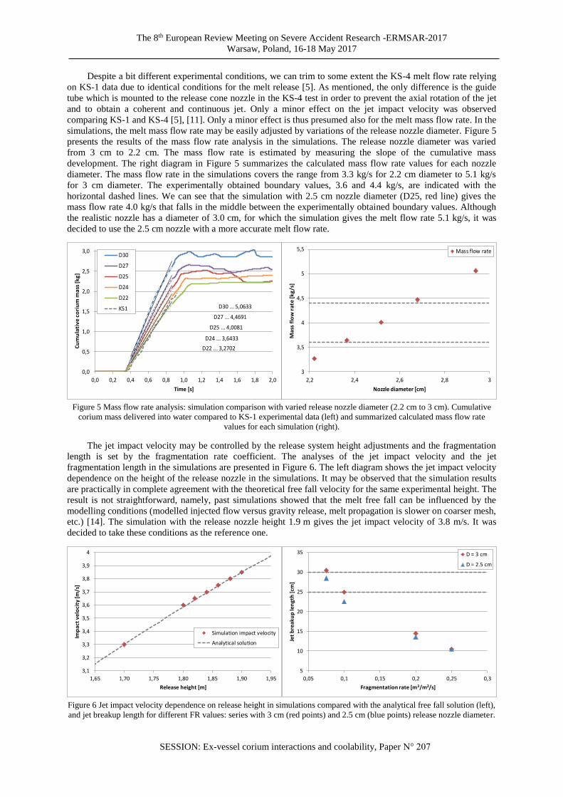
Despite a bit different experimental conditions, we can trim to some extent the KS-4 melt flow rate relying

on KS-1 data due to identical conditions for the melt release [5]. As mentioned, the only difference is the guide

tube which is mounted to the release cone nozzle in the KS-4 test in order to prevent the axial rotation of the jet

and to obtain a coherent and continuous jet. Only a minor effect on the jet impact velocity was observed

comparing KS-1 and KS-4 [5], [11]. Only a minor effect is thus presumed also for the melt mass flow rate. In the

simulations, the melt mass flow rate may be easily adjusted by variations of the release nozzle diameter. Figure 5

presents the results of the mass flow rate analysis in the simulations. The release nozzle diameter was varied

from 3 cm to 2.2 cm. The mass flow rate is estimated by measuring the slope of the cumulative mass

development. The right diagram in Figure 5 summarizes the calculated mass flow rate values for each nozzle

diameter. The mass flow rate in the simulations covers the range from 3.3 kg/s for 2.2 cm diameter to 5.1 kg/s

for 3 cm diameter. The experimentally obtained boundary values, 3.6 and 4.4 kg/s, are indicated with the

horizontal dashed lines. We can see that the simulation with 2.5 cm nozzle diameter (D25, red line) gives the

mass flow rate 4.0 kg/s that falls in the middle between the experimentally obtained boundary values. Although

the realistic nozzle has a diameter of 3.0 cm, for which the simulation gives the melt flow rate 5.1 kg/s, it was

decided to use the 2.5 cm nozzle with a more accurate melt flow rate.

Figure 5 Mass flow rate analysis: simulation comparison with varied release nozzle diameter (2.2 cm to 3 cm). Cumulative

corium mass delivered into water compared to KS-1 experimental data (left) and summarized calculated mass flow rate

values for each simulation (right).

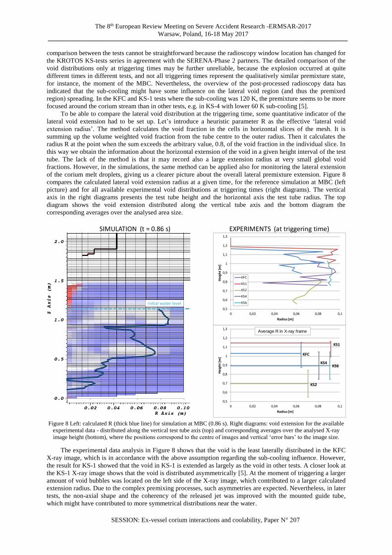
The jet impact velocity may be controlled by the release system height adjustments and the fragmentation

length is set by the fragmentation rate coefficient. The analyses of the jet impact velocity and the jet

fragmentation length in the simulations are presented in Figure 6. The left diagram shows the jet impact velocity

dependence on the height of the release nozzle in the simulations. It may be observed that the simulation results

are practically in complete agreement with the theoretical free fall velocity for the same experimental height. The

result is not straightforward, namely, past simulations showed that the melt free fall can be influenced by the

modelling conditions (modelled injected flow versus gravity release, melt propagation is slower on coarser mesh,

etc.) [14]. The simulation with the release nozzle height 1.9 m gives the jet impact velocity of 3.8 m/s. It was

decided to take these conditions as the reference one.

Figure 6 Jet impact velocity dependence on release height in simulations compared with the analytical free fall solution (left),

and jet breakup length for different FR values: series with 3 cm (red points) and 2.5 cm (blue points) release nozzle diameter.

D30 ... 5,0633

D27 ... 4,4691

D25 ... 4,0081

D24 ... 3,6433

D22 ... 3,2702

0,0

0,5

1,0

1,5

2,0

2,5

3,0

0,0 0,2 0,4 0,6 0,8 1,0 1,2 1,4 1,6 1,8 2,0

Cu

mu

lati

ve

co

riu

m m

ass

[k

g]

Time [s]

D30

D27

D25

D24

D22

KS1

3

3,5

4

4,5

5

5,5

2,2 2,4 2,6 2,8 3

Ma

ss f

low

ra

te [

kg

/s]

Nozzle diameter [cm]

Mass flow rate

3,1

3,2

3,3

3,4

3,5

3,6

3,7

3,8

3,9

4

1,65 1,70 1,75 1,80 1,85 1,90 1,95

Imp

act

ve

loci

ty[m

/s]

Release height [m]

Simulation impact velocity

Analytical solution

5

10

15

20

25

30

35

0,05 0,1 0,15 0,2 0,25 0,3

Jet

bre

aku

p le

ng

th [

cm]

Fragmentation rate [m3/m2/s]

D = 3 cm

D = 2.5 cm




The jet fragmentation (breakup) length analysis is shown in the right diagram in Figure 6. In MC3D

simulations the jet fragmentation length is set by the fragmentation rate coefficient (FR) of the global jet

fragmentation model [8]. Since the jet fragmentation length in the global jet fragmentation model is proportional

to the melt mass (volume) flow rate, two simulations’ series with 3 cm and 2.5 cm nozzle diameter were

performed by varying the FR coefficient. With reducing the melt mass flow rate by narrowing the release nozzle

diameter, the jet fragmentation length shortened a bit while keeping the FR fixed, e.g. at 0.075 m/s. In the

diagram, the range of the preferred jet fragmentation length (25 cm to 30 cm) is depicted with horizontal dashed

lines. The simulation with the release nozzle diameter of 2.5 cm and with FR 0.075 m/s gives the jet

fragmentation length of 28.5 cm, which almost ideally falls within the preferred range. Even more, the values

nearer to 30 cm may be preferred because the jet fragmentation length in the global jet fragmentation model

more corresponds to the ‘point of the full jet fragmentation’ mentioned above. Therefore, the default jet

fragmentation rate coefficient (FR) value, 0.075 m/s, was kept for the reference simulation.

3. Premixing Analysis with Computer Simulation

The reference premixing phase simulation is performed with the calculation conditions summarized in the

table within Figure 4 and with the established melt release system with release nozzle diameter 2.5 cm. The basic

simulation results, the melt propagation and the void fraction development (blue lines), are compared to the

KS-4 experimental results (grey lines) in Figure 7. The vertical dashed lines within the diagrams depict the

typical times of melt bottom contact (MBC): in the simulation at 0.86 s (blue vertical line) and in the experiment

at 1.18 s, which in the KS-4 case corresponds also to the triggering time (grey vertical line). In the left diagram it

may be observed that, after the point of full jet fragmentation in the water, the melt propagation in the simulation

is a bit faster than in the experiment (ZT thermocouples). The perfect melt propagation is not in the main focus

here since it may depend on many various factors. From the simulations’ point of view, the important is the

MBC, which is usually taken as the triggering time for the subsequent explosion simulation. Namely, the

explosion in the KS-4 experiment occurred at the moment of the MBC.

Figure 7 Premixing simulation comparison with experimental data: melt propagation (left), void fraction development (right).

The right diagram in Figure 7 compares the global void fraction development, which is followed in the

whole water section below the initial water level (Total), and the void fraction development measured within the

KS-4 X-ray image window (Frame), which is depicted with the dashed lines. First, it may be observed that the

initial void fraction build-up in the simulations is a bit delayed compared to the experimental void build-up,

which is usually more expressed with the global jet fragmentation model. One reason is that the water level

measurement in the experiment detects also the initial raise of the water surface due to the melt entering the

water. In the simulation with the global jet fragmentation model, the initial void build-up might be improved

with the droplet size, which should be however adjusted together with other premixing and heat transfer

parameters. The droplet size was determined mainly by ‘fitting’ the overall void production, which is the most

indicative process of the heat transfer in given conditions [11]. Second, as up to now, the modelling was

primarily focused on ‘fitting’ the global void fraction, the radioscopy data may provide some additional

information. The interesting fact observed is the general dynamics of the void evolution especially within the

X-ray window, which is expressed by the subsequent rises similar to those in the experiment - in general the void

evolution in the simulation is qualitatively in compliance with the experimental observations. Within the KS-4

X-ray window, which is positioned relatively in the upper area of the test tube (0.7 m to 1.0 m, see Figure 4), the

void fraction is higher than the average (global void) at least up to the MBC.

Additionally, from the post-processed radioscopy data, the provided local data of the void volume fraction

at the triggering time may give us some more insight into the premixture development. Unfortunately, the

0,0

0,2

0,4

0,6

0,8

1,0

1,2

1,4

1,6

1,8

2,0

-0,2 0,0 0,2 0,4 0,6 0,8 1,0 1,2 1,4 1,6 1,8 2,0

Fro

nt

jet

po

siti

on

[m

]

Time [s]

Experiment

Melt Front

water height at 1.15 m

0

0,1

0,2

0,3

0,4

0,5

0,6

0,7

0,0 0,2 0,4 0,6 0,8 1,0 1,2 1,4 1,6 1,8 2,0

Void

frac

tio

n

Time [s]

Exp. Total

Exp. Frame

Sim. Total

Sim. Frame

0,15

0,20

0,25

0,30

0,35

0,40

0,0 0,2 0,4 0,6 0,8 1,0 1,2 1,4 1,6 1,8 2,0

Pre

ssu

re[M

Pa]

Time [s]

Experiment

Pressure

0,0

0,5

1,0

1,5

2,0

2,5

3,0

3,5

0,0 0,2 0,4 0,6 0,8 1,0 1,2 1,4 1,6 1,8 2,0

Dro

ple

t m

ass

[k

g]

Time [s]

Total

Liquid

Active




comparison between the tests cannot be straightforward because the radioscopy window location has changed for

the KROTOS KS-tests series in agreement with the SERENA-Phase 2 partners. The detailed comparison of the

void distributions only at triggering times may be further unreliable, because the explosion occurred at quite

different times in different tests, and not all triggering times represent the qualitatively similar premixture state,

for instance, the moment of the MBC. Nevertheless, the overview of the post-processed radioscopy data has

indicated that the sub-cooling might have some influence on the lateral void region (and thus the premixed

region) spreading. In the KFC and KS-1 tests where the sub-cooling was 120 K, the premixture seems to be more

focused around the corium stream than in other tests, e.g. in KS-4 with lower 60 K sub-cooling [5].

To be able to compare the lateral void distribution at the triggering time, some quantitative indicator of the

lateral void extension had to be set up. Let’s introduce a heuristic parameter R as the effective ‘lateral void

extension radius’. The method calculates the void fraction in the cells in horizontal slices of the mesh. It is

summing up the volume weighted void fraction from the tube centre to the outer radius. Then it calculates the

radius R at the point when the sum exceeds the arbitrary value, 0.8, of the void fraction in the individual slice. In

this way we obtain the information about the horizontal extension of the void in a given height interval of the test

tube. The lack of the method is that it may record also a large extension radius at very small global void

fractions. However, in the simulations, the same method can be applied also for monitoring the lateral extension

of the corium melt droplets, giving us a clearer picture about the overall lateral premixture extension. Figure 8

compares the calculated lateral void extension radius at a given time, for the reference simulation at MBC (left

picture) and for all available experimental void distributions at triggering times (right diagrams). The vertical

axis in the right diagrams presents the test tube height and the horizontal axis the test tube radius. The top

diagram shows the void extension distributed along the vertical tube axis and the bottom diagram the

corresponding averages over the analysed area size.

Figure 8 Left: calculated R (thick blue line) for simulation at MBC (0.86 s). Right diagrams: void extension for the available

experimental data - distributed along the vertical test tube axis (top) and corresponding averages over the analysed X-ray

image height (bottom), where the positions correspond to the centre of images and vertical ‘error bars’ to the image size.

The experimental data analysis in Figure 8 shows that the void is the least laterally distributed in the KFC

X-ray image, which is in accordance with the above assumption regarding the sub-cooling influence. However,

the result for KS-1 showed that the void in KS-1 is extended as largely as the void in other tests. A closer look at

the KS-1 X-ray image shows that the void is distributed asymmetrically [5]. At the moment of triggering a larger

amount of void bubbles was located on the left side of the X-ray image, which contributed to a larger calculated

extension radius. Due to the complex premixing processes, such asymmetries are expected. Nevertheless, in later

tests, the non-axial shape and the coherency of the released jet was improved with the mounted guide tube,

which might have contributed to more symmetrical distributions near the water.

SIMULATION (t = 0.86 s) EXPERIMENTS (at triggering time)

0,5

0,6

0,7

0,8

0,9

1

1,1

1,2

1,3

0 0,02 0,04 0,06 0,08 0,1

He

igh

t [m

]

Radius [m]

KFC

KS1

KS2

KS4

KS6

KFC

KS1

KS2

KS4KS6

0,5

0,6

0,7

0,8

0,9

1

1,1

1,2

1,3

0 0,02 0,04 0,06 0,08 0,1

He

igh

t [m

]

Radius [m]

Average R in X-ray frame

initial water level




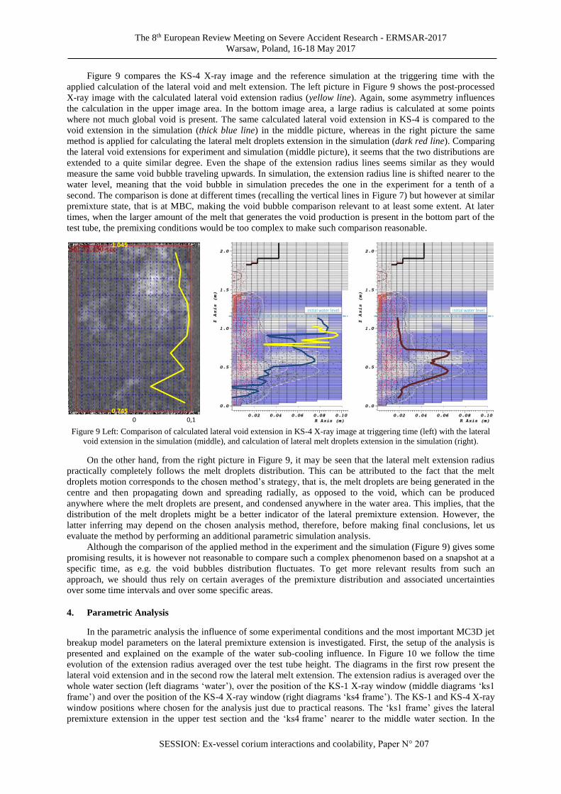
Figure 9 compares the KS-4 X-ray image and the reference simulation at the triggering time with the

applied calculation of the lateral void and melt extension. The left picture in Figure 9 shows the post-processed

X-ray image with the calculated lateral void extension radius (yellow line). Again, some asymmetry influences

the calculation in the upper image area. In the bottom image area, a large radius is calculated at some points

where not much global void is present. The same calculated lateral void extension in KS-4 is compared to the

void extension in the simulation (thick blue line) in the middle picture, whereas in the right picture the same

method is applied for calculating the lateral melt droplets extension in the simulation (dark red line). Comparing

the lateral void extensions for experiment and simulation (middle picture), it seems that the two distributions are

extended to a quite similar degree. Even the shape of the extension radius lines seems similar as they would

measure the same void bubble traveling upwards. In simulation, the extension radius line is shifted nearer to the

water level, meaning that the void bubble in simulation precedes the one in the experiment for a tenth of a

second. The comparison is done at different times (recalling the vertical lines in Figure 7) but however at similar

premixture state, that is at MBC, making the void bubble comparison relevant to at least some extent. At later

times, when the larger amount of the melt that generates the void production is present in the bottom part of the

test tube, the premixing conditions would be too complex to make such comparison reasonable.

Figure 9 Left: Comparison of calculated lateral void extension in KS-4 X-ray image at triggering time (left) with the lateral

void extension in the simulation (middle), and calculation of lateral melt droplets extension in the simulation (right).

On the other hand, from the right picture in Figure 9, it may be seen that the lateral melt extension radius

practically completely follows the melt droplets distribution. This can be attributed to the fact that the melt

droplets motion corresponds to the chosen method’s strategy, that is, the melt droplets are being generated in the

centre and then propagating down and spreading radially, as opposed to the void, which can be produced

anywhere where the melt droplets are present, and condensed anywhere in the water area. This implies, that the

distribution of the melt droplets might be a better indicator of the lateral premixture extension. However, the

latter inferring may depend on the chosen analysis method, therefore, before making final conclusions, let us

evaluate the method by performing an additional parametric simulation analysis.

Although the comparison of the applied method in the experiment and the simulation (Figure 9) gives some

promising results, it is however not reasonable to compare such a complex phenomenon based on a snapshot at a

specific time, as e.g. the void bubbles distribution fluctuates. To get more relevant results from such an

approach, we should thus rely on certain averages of the premixture distribution and associated uncertainties

over some time intervals and over some specific areas.

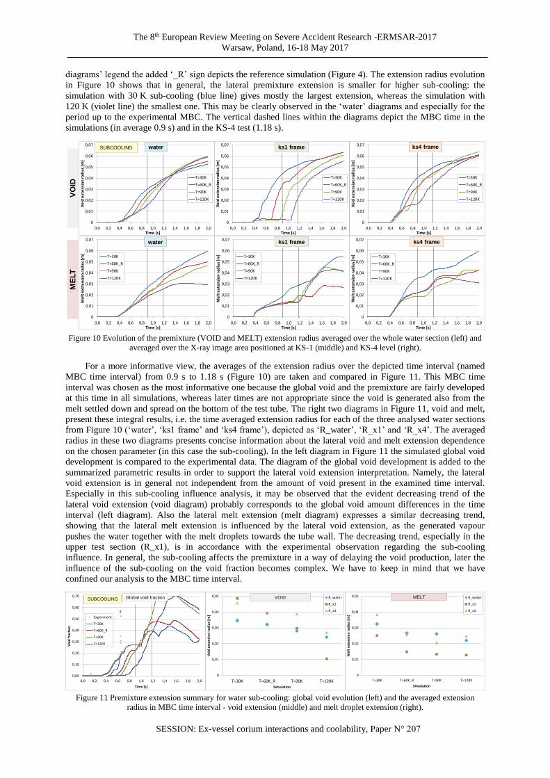
4. Parametric Analysis

In the parametric analysis the influence of some experimental conditions and the most important MC3D jet

breakup model parameters on the lateral premixture extension is investigated. First, the setup of the analysis is

presented and explained on the example of the water sub-cooling influence. In Figure 10 we follow the time

evolution of the extension radius averaged over the test tube height. The diagrams in the first row present the

lateral void extension and in the second row the lateral melt extension. The extension radius is averaged over the

whole water section (left diagrams ‘water’), over the position of the KS-1 X-ray window (middle diagrams ‘ks1

frame’) and over the position of the KS-4 X-ray window (right diagrams ‘ks4 frame’). The KS-1 and KS-4 X-ray

window positions where chosen for the analysis just due to practical reasons. The ‘ks1 frame’ gives the lateral

premixture extension in the upper test section and the ‘ks4 frame’ nearer to the middle water section. In the

0,745

1,045

0 0,1

initial water level initial water level




diagrams’ legend the added ‘_R’ sign depicts the reference simulation (Figure 4). The extension radius evolution

in Figure 10 shows that in general, the lateral premixture extension is smaller for higher sub-cooling: the

simulation with 30 K sub-cooling (blue line) gives mostly the largest extension, whereas the simulation with

120 K (violet line) the smallest one. This may be clearly observed in the ‘water’ diagrams and especially for the

period up to the experimental MBC. The vertical dashed lines within the diagrams depict the MBC time in the

simulations (in average 0.9 s) and in the KS-4 test (1.18 s).

Figure 10 Evolution of the premixture (VOID and MELT) extension radius averaged over the whole water section (left) and

averaged over the X-ray image area positioned at KS-1 (middle) and KS-4 level (right).

For a more informative view, the averages of the extension radius over the depicted time interval (named

MBC time interval) from 0.9 s to 1.18 s (Figure 10) are taken and compared in Figure 11. This MBC time

interval was chosen as the most informative one because the global void and the premixture are fairly developed

at this time in all simulations, whereas later times are not appropriate since the void is generated also from the

melt settled down and spread on the bottom of the test tube. The right two diagrams in Figure 11, void and melt,

present these integral results, i.e. the time averaged extension radius for each of the three analysed water sections

from Figure 10 (‘water’, ‘ks1 frame’ and ‘ks4 frame’), depicted as ‘R_water’, ‘R_x1’ and ‘R_x4’. The averaged

radius in these two diagrams presents concise information about the lateral void and melt extension dependence

on the chosen parameter (in this case the sub-cooling). In the left diagram in Figure 11 the simulated global void

development is compared to the experimental data. The diagram of the global void development is added to the

summarized parametric results in order to support the lateral void extension interpretation. Namely, the lateral

void extension is in general not independent from the amount of void present in the examined time interval.

Especially in this sub-cooling influence analysis, it may be observed that the evident decreasing trend of the

lateral void extension (void diagram) probably corresponds to the global void amount differences in the time

interval (left diagram). Also the lateral melt extension (melt diagram) expresses a similar decreasing trend,

showing that the lateral melt extension is influenced by the lateral void extension, as the generated vapour

pushes the water together with the melt droplets towards the tube wall. The decreasing trend, especially in the

upper test section (R_x1), is in accordance with the experimental observation regarding the sub-cooling

influence. In general, the sub-cooling affects the premixture in a way of delaying the void production, later the

influence of the sub-cooling on the void fraction becomes complex. We have to keep in mind that we have

confined our analysis to the MBC time interval.

Figure 11 Premixture extension summary for water sub-cooling: global void evolution (left) and the averaged extension

radius in MBC time interval - void extension (middle) and melt droplet extension (right).

0

0,01

0,02

0,03

0,04

0,05

0,06

0,07

0,0 0,2 0,4 0,6 0,8 1,0 1,2 1,4 1,6 1,8 2,0

Vo

id e

xte

nsi

on

rad

ius

[m]

Time [s]

T=30K

T=60K_R

T=90K

T=120K

waterSUBCOOLING

0

0,01

0,02

0,03

0,04

0,05

0,06

0,07

0,0 0,2 0,4 0,6 0,8 1,0 1,2 1,4 1,6 1,8 2,0

Vo

id e

xte

nsi

on

rad

ius

[m]

Time [s]

T=30K

T=60K_R

T=90K

T=120K

ks1 frame

0

0,01

0,02

0,03

0,04

0,05

0,06

0,07

0,0 0,2 0,4 0,6 0,8 1,0 1,2 1,4 1,6 1,8 2,0

Vo

id e

xte

nsi

on

rad

ius

[m]

Time [s]

T=30K

T=60K_R

T=90K

T=120K

ks4 frame

0

0,01

0,02

0,03

0,04

0,05

0,06

0,07

0,0 0,2 0,4 0,6 0,8 1,0 1,2 1,4 1,6 1,8 2,0

Me

lt e

xtte

nsi

on

rad

ius

[m]

Time [s]

T=30K

T=60K_R

T=90K

T=120K

water

0

0,01

0,02

0,03

0,04

0,05

0,06

0,07

0,0 0,2 0,4 0,6 0,8 1,0 1,2 1,4 1,6 1,8 2,0

Me

lt e

xten

sio

n r

adiu

s [m

]

Time [s]

T=30K

T=60K_R

T=90K

T=120K

ks1 frame

0

0,01

0,02

0,03

0,04

0,05

0,06

0,07

0,0 0,2 0,4 0,6 0,8 1,0 1,2 1,4 1,6 1,8 2,0

Me

lt e

xten

sio

n r

adiu

s [m

]

Time [s]

T=30K

T=60K_R

T=90K

T=120K

ks4 frame

ME

LT

VO

ID

0,00

0,10

0,20

0,30

0,40

0,50

0,60

0,70

0,0 0,2 0,4 0,6 0,8 1,0 1,2 1,4 1,6 1,8 2,0

Vo

id f

ract

ion

Time [s]

Experiment

Mat1

Mat2_R

Mat3

Mat4

MATERIAL Global void fraction

0,00

0,10

0,20

0,30

0,40

0,50

0,60

0,70

0,0 0,2 0,4 0,6 0,8 1,0 1,2 1,4 1,6 1,8 2,0

Vo

id f

ract

ion

Time [s]

Experiment

T=30K

T=60K_R

T=90K

T=120K

SUBCOOLING Global void fraction

0

0,01

0,02

0,03

0,04

0,05

Mat1 Mat2_R Mat3 Mat4

Vo

id e

xten

sio

n r

adiu

s [m

]

Simulation

R_water

R_x1

R_x4

VOID

0

0,01

0,02

0,03

0,04

0,05

T=30K T=60K_R T=90K T=120K

Vo

id e

xten

sio

n r

adiu

s [m

]

Simulation

R_water

R_x1

R_x4

VOID

0

0,01

0,02

0,03

0,04

0,05


Mel

t ex

ten

sio

n r

adiu

s [m

]

Simulation

R_water

R_x1

R_x4

MELT

0

0,01

0,02

0,03

0,04

0,05

T=30K T=60K_R T=90K T=120K

Mel

t ex

ten

sio

n r

adiu

s [m

]

Simulation

R_water

R_x1

R_x4

MELT




Figure 12 summarizes the results of the premixture extension analyses for the material composition and for

four MC3D specific modelling parameters: coefficient for radial velocity of generated droplets from jet

fragmentation used in global jet fragmentation model (VEJDR), turbulent diffusion terms of melt droplets in

liquid and gas, fragmentation rate coefficient used in global jet fragmentation model (FRGFLM), and melt

droplet Sauter diameter of generated droplets from jet fragmentation used in global jet fragmentation model

(DIACRE). These modelling parameters were chosen for the parametric analysis as they govern the jet breakup

and the premixture extension.

Figure 12 Premixture extension summary: global void evolution (left) and the averaged extension radius in the typical time

interval - void extension (middle) and melt extension (right). Analysis for material composition and other modelling specific

parameters (VEJDR, turbulent diffusion, FRGFLM and DIACRE).

0,00

0,10

0,20

0,30

0,40

0,50

0,60

0,70

0,0 0,2 0,4 0,6 0,8 1,0 1,2 1,4 1,6 1,8 2,0

Vo

id f

ract

ion

Time [s]

Experiment

Mat1

Mat2_R

Mat3

Mat4

MATERIAL Global void fraction

0,00

0,10

0,20

0,30

0,40

0,50

0,60

0,70

0,0 0,2 0,4 0,6 0,8 1,0 1,2 1,4 1,6 1,8 2,0

Vo

id f

ract

ion

Time [s]

Experiment

T=30K

T=60K_R

T=90K

T=120K

SUBCOOLING Global void fraction

0

0,01

0,02

0,03

0,04

0,05


Vo

id e

xte

nsi

on

ra

diu

s [m

]

Simulation

R_water

R_x1

R_x4

VOID

0

0,01

0,02

0,03

0,04

0,05

T=30K T=60K_R T=90K T=120K

Vo

id e

xte

nsi

on

ra

diu

s [m

]

Simulation

R_water

R_x1

R_x4

VOID

0

0,01

0,02

0,03

0,04

0,05


Me

lt e

xte

nsi

on

ra

diu

s [m

]

Simulation

R_water

R_x1

R_x4

MELT

0

0,01

0,02

0,03

0,04

0,05

T=30K T=60K_R T=90K T=120KM

elt

ext

en

sio

n r

ad

ius

[m]

Simulation

R_water

R_x1

R_x4

MELT

0,00

0,10

0,20

0,30

0,40

0,50

0,60

0,70

0,0 0,2 0,4 0,6 0,8 1,0 1,2 1,4 1,6 1,8 2,0

Vo

id f

ract

ion

Time [s]

Experiment

V=0.0

V=0.1

V=0.3

V=0.5_R

V=0.7

V=0.9

V=1.0

VEJDR Global void fraction

0,00

0,10

0,20

0,30

0,40

0,50

0,60

0,70

0,0 0,2 0,4 0,6 0,8 1,0 1,2 1,4 1,6 1,8 2,0

Vo

id f

ract

ion

Time [s]

Experiment

TURB=0.0_R

TURB=0.5

TURB=1.0

TURB=2.0

TURB. DIFFUSION Global void fraction

0,00

0,10

0,20

0,30

0,40

0,50

0,60

0,70

0,0 0,2 0,4 0,6 0,8 1,0 1,2 1,4 1,6 1,8 2,0

Vo

id f

ract

ion

Time [s]

Experiment

FR=0.075_R

FR=0.1

FR=0.2

FR=0.25

FRGFLM Global void fraction

0,00

0,10

0,20

0,30

0,40

0,50

0,60

0,70

0,0 0,2 0,4 0,6 0,8 1,0 1,2 1,4 1,6 1,8 2,0

Vo

id f

ract

ion

Time [s]

Experiment

D=1.5 mm

D=2 mm

D=2.5 mm _R

D=3 mm

D=4 mm

DIACRE Global void fraction

0

0,01

0,02

0,03

0,04

0,05

TURB=0.0_R TURB=0.5 TURB=1.0 TURB=2.0

Vo

id e

xte

nsi

on

ra

diu

s [m

]

Simulation

R_water

R_x1

R_x4

VOID

0

0,01

0,02

0,03

0,04

0,05

D=1.5 mm D=2 mm D=2.5 mm _R D=3 mm D=4 mm

Vo

id e

xte

nsi

on

ra

diu

s [m

]

Simulation

R_water

R_x1

R_x4

VOID

0

0,01

0,02

0,03

0,04

0,05

V=0.0 V=0.1 V=0.3 V=0.5_R V=0.7 V=0.9 V=1.0M

elt

ext

en

sio

n r

ad

ius

[m]

Simulation

R_water

R_x1

R_x4

MELT

0

0,01

0,02

0,03

0,04

0,05

TURB=0.0_R TURB=0.5 TURB=1.0 TURB=2.0

Me

lt e

xte

nsi

on

ra

diu

s [m

]

Simulation

R_water

R_x1

R_x4

MELT

0

0,01

0,02

0,03

0,04

0,05

FR=0.075_R FR=0.1 FR=0.2 FR=0.25

Me

lt e

xte

nsi

on

ra

diu

s [m

]

Simulation

R_water

R_x1

R_x4

MELT

0

0,01

0,02

0,03

0,04

0,05

D=1.5 mm D=2 mm D=2.5 mm _R D=3 mm D=4 mm

Me

lt e

xte

nsi

on

ra

diu

s [m

]

Simulation

R_water

R_x1

R_x4

MELT

0

0,01

0,02

0,03

0,04

0,05

V=0.0 V=0.1 V=0.3 V=0.5_R V=0.7 V=0.9 V=1.0

Vo

id e

xte

nsi

on

ra

diu

s [m

]

Simulation

R_water

R_x1

R_x4

VOID

0

0,01

0,02

0,03

0,04

0,05

FR=0.075_R FR=0.1 FR=0.2 FR=0.25

Vo

id e

xte

nsi

on

ra

diu

s [m

]

Simulation

R_water

R_x1

R_x4

VOID




In the material composition analysis in Figure 12 all four prototypic SERENA-KROTOS KS material

compositions ‘Mat1’-‘Mat4’ were considered, with significantly increasing solidification temperature range and

typical slightly decreasing liquidus temperature from ‘Mat1’ to ‘Mat4’ [4], [11], [13]. The analysis shows that

the lateral premixture (void and melt) extension typically slightly reduces with increasing solidification

temperature range and/or with decreasing material melting temperature (see first row of diagrams in Figure 12).

The influence is probably related to the global void fraction, which typically decreases when the solidification

temperature range increases and/or the melting temperature decreases due to the faster initial cooling related to

the lower solidification temperatures, as explained in the sub-cooling analysis.

In the modelling parameter analysis (Figure 12), first a distinctive increasing trend of the lateral premixture

extension is observed for the radial melt droplet velocity coefficient - VEJDR. However, this trend is clearly

reflected only in the lateral melt extension. The lateral void extension initially increases and later expresses a

slightly decreasing trend. The reason is probably because a too diluted melt droplet field is not capable to

produce a large void in the outer regions. For the value of the turbulent diffusion term the decreasing trend of the

lateral void extension probably corresponds to the decreasing global void, which is related to the melt droplet

field dilution. The lateral melt extension expresses an initial increase and later a rather stochastic behaviour. For

the jet fragmentation rate coefficient (FRGFLM) a stochastic influence on the lateral premixture extension may

be observed. However, an interesting slightly increasing void extension may be observed near the water level

(R_x1). For the melt droplet Sauter diameter (DIACRE) the significantly decreasing trend of the lateral

premixture extension probably corresponds also to the decreasing global void.

Additional investigations were carried out to support the results of the parametric analysis. First, the above

parametric analysis was repeated for a bit shorter and earlier time interval, 0.85 s – 1.0 s, in order to avoid the

influence of the potentially settled down melt. Within the previously considered later time interval, in many

simulations after the MBC a small amount of void was already produced by the melt on the test section bottom.

Except the general reduction of the lateral premixture extension within the earlier time interval, no major

differences were observed.

5. Conclusions

The innovative X-ray radioscopy experimental data of the KROTOS SERENA-Phase 2 tests provide

important new insight into the complex premixing process and opened various possibilities for the improvement

of the analytical work and the key FCI-phenomena understanding. Because from the X-ray images the local data

of the premixed region may be obtained, the performed study with the MC3D is focused mainly on the lateral

distribution of the premixture along the test section. Based on the post-processed X-ray radioscopy data an

appropriate model of the melt release system could be developed, resulting in the experimentally observed melt

jet inlet conditions, which is the prerequisite for reliable experiment calculations. The X-ray radioscopy data

enabled a more accurate determination of the jet breakup length and the premixing fragmentation process, and it

was shown that the jet breakup length is correctly predicted with the global jet breakup model, applying the

default value of the jet fragmentation rate parameter.

The comprehensive parametric analysis, investigating the influence various experimental conditions and

MC3D jet breakup model parameters on the lateral premixture extension, revealed important features. The

analysis confirmed the experimental X-ray data indications that the lateral premixture extension decreases with

increasing water sub-cooling. It turned out that the lateral premixture extension is driven mainly by the amount

of the local produced vapour, as the emerging vapour pushes the water together with the melt droplets towards

the tube wall. Thus the influence of an individual parameter on the lateral premixture extension is not

straightforward. If initially the melt droplets are focused mainly around the centre, there is a high potential of

energy to produce the void, that can consequently significantly extend the premixture. On the other hand, if the

melt droplets initially spread in a wider water region, e.g. due to a higher radial droplet velocity or due to a larger

turbulent diffusion, less void is produced by the droplets in the abundant amount of surrounding water,

consequently resulting in a lower overall premixture extension. However, the amount of the void produced is

determined also by various other factors, e.g. the droplets size, which consequently contribute to the examined

lateral premixture extension.. Therefore, it is not straightforward to establish the appropriate modelling

parameters even if some local experimental data is available. The benefits of the KROTOS X-ray radioscopy

system offer quite some challenges that may be considered in further analytical and experimental activities. To

be able to better characterize the premixture, especially the melt droplets distribution, and the premixing process,

experiments with a larger X-ray window, ideally covering the entire test section, and with higher spatial

resolution would be beneficial for better understanding and modelling of FCI and SE phenomena.




Acknowledgments

The authors gratefully thank OECD for organizing the SERENA program and all the countries participating in

the SERENA-Phase 2 program. The authors acknowledge the financial support of the Slovenian Research

Agency within the research program P2-0026 and the cooperative CEA-JSI research project (contract number

BI-FR/CEA/15-17-006) for the work performed at the Jožef Stefan Institute.

References

[1] G. Berthoud, Vapour Explosions, Ann Rev Fluid Mech, 32, pp. 573-611, 2000.

[2] T.G. Theoufanous, The Study of Steam Explosions in Nuclear Systems, Nucl. Eng. Des. 155, pp. 1-26,

1995.

[3] M. Leskovar, M. Uršič, Estimation of Ex-Vessel Steam Explosion Pressure Loads, Nucl. Eng. Des. 239, pp.

2444-2458, 2009.

[4] S. W. Hong, P. Piluso, M. Leskovar, Status of the OECD-SERENA Project for the Resolution of Ex-Vessel

Steam Explosion Risks, J En Power Eng, 7, pp. 423-431, 2013.

[5] N. Cassiaut-Louis, D. Grishchenko, "KROTOS Radioscopy Data Analysis for KFC Test and KS-Series

Tests", Technical report CEA/DEN, 2016.

[6] D. Grishchenko et al., "X-Ray Measurements of the Premixing Phase: Analysis with KIWI Software",

conference presentation, SERENA Project Seminar, Cadarache, 2012.

[7] C. Brayer, P. Piluso, N. Cassiaut-Louis, D. Grishchencko, "Application of X-Ray radioscopy for

investigations of the 3-phase-mixture resulting from the fragmentation of a high temperature molten

material jet in water", 8th International Conference on Multiphase Flow, ICMF, Jeju, Korea, 2013.

[8] R. Meignen et al., The challenge of modeling fuel-coolant interaction: Part I - Premixing, Nucl Eng Des,

280, pp. 511-527, 2014.

[9] R. Meignen, B. Raverdy, S. Picchi, J. Lamome, The challenge of modeling fuel-coolant interaction: Part II

- Steam explosion, Nucl Eng Des, 280, pp. 528-541, 2014.

[10] J-M. Bonnet et al., "KROTOS KS-1 Test Data Report", CEA, Cadarache, 2009.

[11] V. Centrih, M. Leskovar, "Analysis of X-Ray Images in SERENA KROTOS Experiments", IJS-DP-12176,

JSI, Ljubljana, 2016.

[12] D. Grishchenko et al., "KROTOS KS-4 Test Data Report", CEA, Cadarache, 2011.

[13] R. Meignen et al., "SERENA-Phase 2: Post Calculations for TROI TS-4, Pre-calculation of TROI TS-5 and

TS-6 Analysis of Impact of Melt Properties on FCI", IRSN, Clamart, 2012.

[14] M. Leskovar, M. Uršič, "Simulation of First SERENA KROTOS Steam Explosion Experiment",

Proceedings of ICAPP ‘09, Tokyo, Japan, May 10-14, paper 9001, 2009.

MC3D Premixing Analysis using X-Ray Radioscopy ... Paper - MC3D... · MC3D Premixing Analysis using X-Ray ... The 8th European Review Meeting on Severe Accident Research ... smaller

Documents