Maximum Likelihood Estimation in Latent Class Models …arinaldo/papers/Fienberg_Hersh_Rinaldo_Zhou_20… · Maximum Likelihood Estimation in Latent Class Models For Contingency Table

Maximum Likelihood Estimation in Latent

Class Models For Contingency Table Data

Stephen E. FienbergDepartment of Statistics, MachineLearning Department and Cylab

Carnegie Mellon UniversityPittsburgh, PA 15213-3890 USA

Patricia HershDepartment of Mathematics

Indiana UniversityBloomington, IN 47405-7000 USA

Alessandro RinaldoDepartment of Statistics

Carnegie Mellon UniversityPittsburgh, PA 15213-3890 USA

Yi ZhouMachine Learning DepartmentCarnegie Mellon University

Pittsburgh, PA 15213-3890 USA

Contents

1 page 11.1 Abstract 11.2 Introduction 31.3 Latent Class Models for Contingency Tables 41.4 Geometric Description of Latent Class Models 71.5 Examples Involving Synthetic Data 12

1.5.1 Effective Dimension and Polynomials 121.5.2 The 100 Swiss Franks Problem 15

1.6 Two Applications 321.6.1 Example: Michigan Influenza 321.6.2 Data From the National Long Term Care

Survey 331.7 On Symmetric Tables and the MLE 37

1.7.1 Introduction and Motivation 381.7.2 Preservation of Marginals and Some Conse-

quences 411.7.3 The 100 Swiss Franks Problem 44

1.8 Conclusions 471.9 Acknowledgments 48

References 49

iii

1

1.1 Abstract

Statistical models with latent structure have a history going back to the1950s and have seen widespread use in the social sciences and, morerecently, in computational biology and in machine learning. Here westudy the basic latent class model proposed originally by the sociologistPaul F. Lazarfeld for categorical variables, and we explain its geometricstructure. We draw parallels between the statistical and geometric prop-erties of latent class models and we illustrate geometrically the causesof many problems associated with maximum likelihood estimation andrelated statistical inference. In particular, we focus on issues of non-identifiability and determination of the model dimension, of maximiza-tion of the likelihood function and on the effect of symmetric data. Weillustrate these phenomena with a variety of synthetic and real-life ta-bles, of different dimensions and complexities. Much of the motivationfor this work stems from the “100 Swiss Franks” problem, which weintroduce and describe in detail.

1

Contents

2

1.2 Introduction 3

1.2 Introduction

Latent class (LC) or latent structure analysis models were introducedin the 1950s in the social science literature to model the distribution ofdichotomous attributes based on a survey sample from a population ofindividuals organized into distinct homogeneous classes according to anunobservable attitudinal feature. See Anderson (1954), Gibson (1955),Madansky (1960) and, in particular, Henry and Lazarfeld (1968). Thesemodels were later generalized in Goodman (1974), Haberman (1974),Clogg and Goodman (1984) as models for the marginal distribution of aset of manifest categorical variables, assumed to be conditionally inde-pendent given an unobservable or latent categorical variable, buildingupon the then recently developed literature on log-linear models forcontingency tables. More recently, latent class models have been de-scribed and studied as special cases of a larger class of directed acyclicgraphical models with hidden nodes, sometimes referred to as Bayesnetworks, or causal models. See, e.g., Lauritzen (1996), Cowell et al.(1999), Humphreys and Titterington (2003) and, in particular, Geigeret al. (2001). A number of recent papers have established fundamentalconnections between the statistical properties of latent class models andtheir algebraic and geometric features. See Settimi and Smith (1998,2005), Smith and Croft (2003), Rusakov and Geiger (2005),Watanabe(2001) and Garcia et al. (2005).

Despite these recent important theoretical advances, the fundamen-tal statistical tasks of estimation, hypothesis testing and model selec-tion remain surprisingly difficult and, in some cases, infeasible, even forsmall models. Nonetheless, LC models are widely used and there is a“folklore” associated with estimation in various computer packages im-plementing algorithms such as EM for estimation purposes, e.g., see Ue-bersax (2006a,b).

The goal of this article is two-fold. First, we offer a simplified geomet-ric and algebraic description of LC models and draw parallels betweentheir statistical and geometric properties. The geometric framework en-joys notable advantages over the traditional statistical representationand, in particular, offers natural ways of representing singularities andnon-identifiability problems. Furthermore, we argue that the many sta-tistical issues encountered in fitting and interpreting LC models are areflection of complex geometric attributes of the associated set of proba-bility distributions. Second, we illustrate with examples, most of whichquite small and seemingly trivial, some of the computational, statistical

4 Contents

and geometric challenges that LC models pose. In particular, we focus onissues of non-identifiability and determination of the model dimension,of maximization of the likelihood function and on the effect of symmetricdata. We also show how to use symbolic software from computationalalgebra to obtain a more convenient and simpler parametrization andfor unravelling the geometric features of LC models. These strategiesand methods may carry over to more complex latent structure models,such as in Bandeen-Roche et al. (1997).

In the next section, we describe the basic latent class model and itsstatistical properties and, in Section 1.4, we discuss the geometry of themodels. In Section 1.5, we turn to our examples exemplifying the identi-fiability issue and the complexity of the likelihood function, with a novelfocus on the problems arising from symmetries in the data. In section1.6, we present some computational results for two real-life examples, ofsmall and very large dimension. In the final section1.7 we investigatein a theoretical fashion the effect of symmetry in the data on maximumlikelihood estimation and derive some results towards the proof of the“100 Swiss Franks” problem from section 1.5.

1.3 Latent Class Models for Contingency Tables

Consider k categorical variables, X1, . . . , Xk, where each Xi takes valueon the finite set [di] ≡ {1, . . . , di}. Letting D =

⊗ki=1[di], RD is the

vector space of k-dimensional arrays of the format d1 × . . . × dk, witha total of d =

∏i di entries. The cross-classification of N indepen-

dent and identically distributed realizations of (X1, . . . , Xk) produces arandom integer-valued vector n ∈ RD, whose coordinate entry nii,...,ikcorresponds to the number of times the label combination (i1, . . . , ik)is observed in the sample, for each (i1, . . . , ik) ∈ D. The table n hasa Multinomial(N,p) distribution, where p is a point in the (d − 1)-dimensional probability simplex ∆d−1 with coordinates

pi1,...,ik = Pr {(X1, . . . , Xk) = (i1, . . . , ik)} , (i1, . . . , ik) ∈ D.

Let H be an unobservable latent variable, defined on the set [r] ={1, . . . , r}. In its most basic version, also known as the naive Bayesmodel, the LC model postulates that, conditional on H, the variablesX1, . . . , Xk are mutually independent. Specifically, the joint distribu-tions of X1, . . . , Xk and H form the subset V of the probability simplex

1.3 Latent Class Models for Contingency Tables 5

∆dr−1 consisting of points with coordinates

pi1,...,ik,h = p(h)1 (i1) . . . p(h)

k (ik)λh, (i1, . . . , ik, h) ∈ D × [r], (1.1)

where λh is the marginal probability Pr{H = h} and p(h)l (il) is the

conditional marginal probability Pr{Xl = il|H = h}, which we assumeto be strictly positive for each h ∈ [r] and (i1, . . . , ik) ∈ D.

The log-linear model specified by the polynomial mappings (1.1) is adecomposable graphical model (see, e.g, Lauritzen, 1996) and V is theimage set of a homeomorphism from the parameter space

Θ ≡{θ: θ = (p(h)

1 (i1) . . . p(h)k (ik), λh), (i1, . . . , ik, h) ∈ D × [r]

}=

⊗i ∆di−1 ×∆r−1,

so that global identifiability is guaranteed. The remarkable statisticalproperties of this type of models and the geometric features of the set Vare well understood. Statistically, equation (1.1) defines a linear expo-nential family of distributions, though not in its natural parametrization.The maximum likelihood estimates, or MLEs, of λh and p(h)

l (il) exist ifand only if the minimal sufficient statistics, i.e., the empirical joint dis-tributions of (Xi, H) for i = 1, 2, . . . , k, are strictly positive and are givenin closed form as rational functions of the observed two-way marginaldistributions of Xi and H for i = 1, 2, . . . , k. The log-likelihood func-tion is strictly concave and the maximum is always attainable, possiblyon the boundary of the parameter space. Furthermore, the asymptotictheory of goodness-of-fit testing is fully developed.

Geometrically, we can obtain the set V as the intersection of ∆dr−1

with an affine variety (see, e.g., Cox et al., 1996) consisting of the solu-tions set of a system of r

∏i

(di

2

)homogeneous square-free polynomials.

For example, when k = 2, each of these polynomials take the form ofquadric equations of the type

pi1,i2,hpi′1,i′2,h = pi′1,i2,hpi1,i′2,h, (1.2)

with i1 6= i′1, i2 6= i′2 and for each fixed h. Provided the probabilitiesare strictly positive, equations of the form (1.2) specify conditional oddsratio of 1, for every pair (Xi, Xi′) given H = h. Furthermore, for eachgiven h, the coordinate projections of the first two coordinates of thepoints satisfying (1.2) trace the surface of independence inside the sim-plex ∆d−1. The strictly positive points of V form a smooth manifoldwhose dimension is r

∏i(di − 1) + (r − 1) and whose co-dimension cor-

responds to the number of degrees of freedom. The singular points of V

6 Contents

all lie on the boundary of the simplex ∆dr−1 and identify distributionswith degenerate probabilities along some coordinates. More generally,the singular locus of V can be described similarly in terms of its stratifiedcomponents, whose dimensions and co-dimensions can also be computedexplicitly.

Under the LC model, the variable H is unobservable and the newmodel H is a r-class mixture over the exponential family of distribu-tions prescribing mutual independence among the manifest variablesX1, . . . , Xk. Geometrically, H is the set of probability vectors in ∆d−1

obtained as the image of the marginalization map from ∆dr−1 onto ∆d−1

which consists of taking the sum over the coordinate corresponding tothe latent variable. Formally, H is made up of all probability vectorsin ∆d−1 with coordinates satisfying the accounting equations (see, e.g.,Henry and Lazarfeld, 1968)

pi1,...,ik =∑h∈[r]

pi1,...,ik,h =∑h∈[r]

p(h)1 (i1) . . . p(h)

k (ik)λh, (1.3)

where (i1, . . . , ik, h) ∈ D × [r].Despite being expressible as a convex combination of very well-behaved

models, even the simplest form of the LC model (1.3) is far from beingwell-behaved and, in fact, shares virtually none of the properties of thestandard log-linear models. In particular, the latent class models spec-ified by equations (1.3) do not define exponential families, but insteadbelong to a broader class of models called stratified exponential families(see Geiger et al., 2001), whose properties are much weaker and less wellunderstood. The minimal sufficient statistics for an observed table nare the observed counts themselves and we can achieve no data reduc-tion via sufficiency. The model may not be identifiable, because for agiven p ∈ ∆d−1 satisfying (1.3), there may be a subset of Θ, known asthe non-identifiable space, consisting of parameter points all satisfyingthe same accounting equations. The non-identifiability issue has in turnconsiderable repercussions on the determination of the correct numberof degrees of freedom for assessing model fit and, more importantly, onthe asymptotic properties of standard model selection criteria (e.g. like-lihood ratio statistic and other goodness-of-fit criteria such as BIC, AIC,etc), whose applicability and correctness may no longer hold.

Computationally, maximizing the log-likelihood can be a rather la-borious and difficult task, particularly for high dimensional tables, dueto lack of concavity, the presence of local maxima and saddle points,and singularities in the observed Fisher information matrix. Geometri-

1.4 Geometric Description of Latent Class Models 7

cally, H is no longer a smooth manifold in the relative interior of ∆d−1,with singularities even at probability vectors with strictly positive coor-dinates, as we show in the next section. The problem of characterizingthe singular locus of H and of computing the dimensions of its stratifiedcomponents (and of the tangent spaces and tangent cones of its singularpoints) is of statistical importance: singularity points of H are probabil-ity distributions of lower complexity, in the sense that they are specifiedby lower-dimensional subsets of Θ, or, loosely speaking, by less param-eters. Because the sample space is discrete, although the singular locusof H has typically Lebesgue measure zero, there is nonetheless a positiveprobability that the maximum likelihood estimates end up being eithera singular point in the relative interior of the simplex ∆d−1 or a pointon the boundary. In both cases, standard asymptotics for hypothesistesting and model selection fall short.

1.4 Geometric Description of Latent Class Models

In this section, we give a geometric representation of latent class models,summarize existing results and point to some of the relevant mathemat-ical literature. For more details, see Garcia et al. (2005) and Garcia(2004).

The latent class model defined by (1.3) can be described as the setof all convex combinations of r-tuple of points lying on the surface ofindependence inside ∆d−1. Formally, let

σ: ∆d1−1 × . . .×∆dk−1 → ∆d−1

(p1(i1), . . . , pk(ik)) 7→∏j pj(ij)

be the map sending the vectors of marginal probabilities into the k-dimensional array of joint probabilities for the model of complete inde-pendence. The set S ≡ σ(∆d1−1 × . . . ×∆dk−1) is a manifold in ∆d−1

known in statistics as the surface of independence and in algebraic ge-ometry (see, e.g. Harris, 1992) as (the intersection of ∆d−1 with) theSegre embedding of Pd1−1 × . . . × Pdk−1 into Pd−1. The dimension ofS is

∏i(di − 1), i.e., the dimension of the corresponding decomposable

model of mutual independence. The set H can then be constructedgeometrically as follows. Pick any combination of r points along thehyper-surface S, say p(1), . . . ,p(r), and determine their convex hull, i.e.the convex set consisting of all points of the form

∑h p(h)λh, for some

choice of (λ1, . . . , λr) ∈ ∆r−1. The coordinates of any point in this newsubset satisfy, by construction, the accounting equations (1.3). In fact,

8 Contents

the closure of the union of all such convex hulls is precisely the latentclass model H. In algebraic geometry, H would be described as the in-tersection of ∆d−1 with the r-th secant variety of the Segre embeddingmentioned above.

Fig. 1.1. Surface of independence for the 2× 2 table with 3 secant lines.

Example 1.4.1 The simplest example of a latent class model is for a 2×2 table with one latent variable with r = 2. The surface of independence,i.e. the intersection of the simplex ∆3 with the Segre variety, is shownin Figure 1.1. The secant variety for this latent class model is the unionof all the secant lines, i.e. the lines connecting any two distinct pointslying on the surface of independence. Figure 1.1 displays three suchsecant lines. It is not too hard to picture that the union of all suchsecant lines is the enveloping simplex ∆3 and, therefore, H fills up allthe available space (for formal arguments, see Catalisano et al., 2002,Proposition 2.3).

The model H is not a smooth manifold. Instead, it is a semi-algebraicset (see, e.g., Benedetti, 1990), clearly singular on the boundary of thesimplex, but also at strictly positive points along the (r − 1)st secantvariety (both of Lebesgue measure zero). This means that the model is


singular at all points in H which satisfy the accounting equations withone or more of the λh’s equal to zero. In Example 1.4.1 above, the surfaceof independence is a singular locus for the latent class model. From thestatistical viewpoint, singular points of H correspond to simpler modelsfor which the number of latent classes is less than r (possibly 0). Asusual, for these points one needs to adjust the number of degrees offreedom to account for the larger tangent space.

Unfortunately, we have no general closed-form expression for comput-ing the dimension of H and the existing results only deal with specificcases. Simple considerations allow us to compute an upper bound for thedimension of H, as follows. As Example 1.4.1 shows, there may be in-stances for whichH fills up the entire simplex ∆d−1, so that d−1 is an at-tainable upper bound. Counting the number of free parameters in (1.3),we can see that this dimension cannot exceed r

∑i(di − 1) + r − 1, (c.f.

Goodman, 1974, page 219). This number, the standard dimension, isthe dimension of the fully observable model of conditional independence.Incidentally, this value can be determined mirroring the geometric con-struction of H as follows (c.f. Garcia, 2004). The number r

∑i(di − 1)

arises from the choice of r points along the∑i(di − 1)-dimensional sur-

face of independence, while the term r − 1 accounts for the number offree parameters for a generic choice of (λ1, . . . , λr) ∈ ∆r−1. Therefore,we conclude that the dimension of H is bounded by

min

{d− 1, r

∑i

(di − 1) + r − 1

}, (1.4)

a value known in algebraic geometry as the expected dimension the va-riety H.

Cases of latent class models with dimension strictly smaller than theexpected dimension have been known for a long time. In the statisti-cal literature, Goodman (1974) noticed that the latent class models for4 binary observable variables and a 3-level latent variable, whose ex-pected dimension is 14, has dimension 13. In algebraic geometry, secantvarieties with dimension smaller than the expected dimension (1.4) arecalled deficient (e.g., see Harris, 1992). In particular, Exercise 11.26 inHarris (1992) gives an example of a deficient secant variety, which cor-responds to a LC model for a 2-way table with a binary latent variable.In this case, the deficiency is 2, as is demonstrated below in equation(1.5). The true or effective dimension of a latent class model, i.e. thedimension of the semi-algeraic set H representing it, is crucial for estab-

10 Contents

lishing identifiability and for computing correctly the number of degreesof freedom. In fact, if a model is deficient, then the pre-image of eachprobability array in H arising from the accounting equations is a subset(in fact, a variety) of Θ called the non-dentifiable subspace, with dimen-sion exactly equal to the deficiency itself. Therefore, a deficient model isnon-identifiable, with adjusted degrees of freedom equal to the numberof degrees of freedom for the observable graphical model plus the valueof the deficiency.

The effective dimension of H is equal to the maximal rank of theJacobian matrix for the polynomial mapping from Θ into H given co-ordinatewise by (1.3). Geiger et al. (2001) showed that this value isequal to the dimension of H almost everywhere with respect to the Leb-segue measure, provided the Jacobian is evaluated at strictly positiveparameter points θ, and used this result to devise a simple algorithm tocompute numerically the effective dimension.

More recently, in the algebraic-geometry literature, Catalisano et al.(2002, 2003) have obtained explicit formulas for the effective dimensionsof some secant varieties which are of statistical interest. In particular,they show that for k = 3 and r ≤ min{d1, d2, d3}, the latent class modelhas the expected dimension and is identifiable. On the other hand,assuming d1 ≤ d2 ≤ . . . ≤ dk, H is deficient when

∏k−1i=1 di −

∑k−1i=1 (di −

1) ≤ r ≤ min{dk,∏k−1i=1 di − 1

}. Finally, under the same conditions, H

is identifiable when 12

∑i(di−1)+1 ≥ max{dk, r}. In general, obtaining

bounds and results of this type is highly non-trivial and is an open areaof research.

In the remainder of the paper, we will focus on simpler latent classmodels for tables of dimension k = 2 and illustrate with examples the re-sults mentioned above. For latent class models on two-way tables, thereis an alternative, quite convenient way of describing H by representingeach p in ∆d−1 as a d1 × d2 matrix and the map σ as a vector product.In fact, each point p in S is a rank one matrix obtained as p1p>2 , wherep1 ∈ ∆d1−1 and p2 ∈ ∆d1−2 are the appropriate marginal distributionsof X1 and X2. Then, the accounting equations for a latent class modelswith r levels become

p =∑h

p(h)1 (p(h)

2 )>λh, (p1,p2, (λ1, . . . , λr)) ∈ ∆d1−1×∆d2−1×∆r−1

i.e. the matrix p is a convex combination of r rank 1 matrices lying onthe surface of independence. Therefore, all points in H are non-negativematrices with entries summing to one and with rank at most r. This


simple observation allows one to compute the effective dimension of Hfor 2-way tables as follows. In general, a real valued d1 × d2 matrixhas rank r or less if and only if the homogeneous polynomial equationscorresponding to all of its (r + 1)× (r + 1) minors all vanish. Providedk < min{d1, d2}, on Rd1×Rd2 , the zero locus of all such equations form adeterminantal variety of co-dimension (d1− r)(d2− r) (c.f. Harris, 1992,Proposition 12.2) and hence has dimension r(d1 + d2)− r2. Subtractingthis value from the expected dimension (1.4), and taking into accountthe fact that all the points lie inside the simplex, we obtain

r(d1 + d2 − 2) + r − 1−(r(d1 + d2)− r2 − 1

)= r(r − 1). (1.5)

This number is also the difference between the dimension of the (fullyidentifiable, i.e. of expected dimension) graphical model of conditionalindependence X1 and X2 given H, and the deficient dimension of thelatent class model obtained by marginalizing over the variable H.

The study of higher dimensional tables is still an open area of re-search. The mathematical machinery required to handle larger dimen-sions is considerably more complicated and relies on the notions ofhigher-dimensional tensors, rank tensors and non-negative rank tensors,for which only partial results exist. See Kruskal (1975), Cohen and Roth-blum (1993) and Strassen (1983) for details. Alternatively, Mond et al.(2003) conduct an algebraic-topological investigation of the topologicalproperties of stochastic factorization of stochastic matrices representingmodels of conditional independence with one hidden variable and All-man and Rhodes (2006, 2007) explore an overlapping set of problemsframed in the context of trees with latent nodes and branches.

The specific case of k-way tables with 2 level latent variables is a fortu-nate exception, for which the results for 2-way tables just described ap-ply. In fact, Landsberg and Manivel (2004) show that that these modelsare the same as the corresponding model for any two-dimensional tableobtained by any “flattening” of the d1 × . . . × dk-dimensional array ofprobabilities p into a two-dimensional matrix. Flattening simply meanscollapsing the k variables into two new variables with f1 and f2 levels,and re-organizing the entries of the k-dimensional tensor p ∈ ∆d−1 intoa f1× f1 matrix accordingly, where, necessarily, f1 + f2 =

∑i di. Then,

H is the determinantal variety which is the zero set of all 3 × 3 sub-determinants of the matrix obtained by any such flattening. The secondexample in Section 1.5.1 below illustrates this result.

12 Contents

1.5 Examples Involving Synthetic Data

We further elucidate the non-identifiability phenomenon from the alge-braic and geometric point of view, and the multi-modality of the log-likelihood function issue using small synthetic examples. In particular,in the “100 Swiss Franks” problem below, we embark on a exhaustivestudy of a table with symmetric data and describe the effects of suchsymmetries on both the parameter space and the log-likelihood func-tion. Although those examples treat simplest cases of LC models, theyalready exhibit considerable statistical and geometric complexity.

1.5.1 Effective Dimension and Polynomials

We show how it is possible to take advantage of the polynomial natureof equations (1.3) to gain further insights into the algebraic propertiesof distributions obeying latent class models. All the computations thatfollow were made in SINGULAR (Greuel et al., 2005) and are described indetails, along with more examples, in Zhou (2007). Although in principlesymbolic algebraic software allows one to compute the set of polynomialequations that fully characterize LC models and their properties, this isstill a difficult and costly task that can be accomplished only for smallermodels.

The accounting equations (1.3) determine a polynomial mapping f : Θ→∆d−1 given by

(p1(i1) . . . pk(ik), λh) 7→∑h∈[r]

p1(i1) . . . pk(ik)λh, (1.6)

so that the latent class model is analytically defined as its image, i.e.H = f(Θ). Then, following the geometry-algebra dictionary princi-ple (see, e.g., Cox et al., 1996), the problem of computing the effectivedimension of H can in turn be geometrically cast as a problem of com-puting the dimension of the image of a polynomial map. We illustratehow this representation offers considerable advantages with some smallexamples.

Consider a 2×2×2 table with r = 2 latent classes. From Proposition2.3 in Catalisano et al. (2002), the latent class models with 2 classes and3 manifest variables are identifiable. The standard dimension, i.e. thedimension of the parameter space Θ is r

∑i(di − 1) + r − 1 = 7, which

coincides with the dimension of the enveloping simplex ∆7. Althoughthis condition implies that the number of parameters to estimate is nolarger than the number of cells in the table, a case which, if violated,

1.5 Examples Involving Synthetic Data 13

would entail non-identifiability, it does not guarantee that the effectivedimension is also 7. This can be verified by checking that the symbolicrank of the Jacobian matrix of the map (1.6) is indeed 7, almost ev-erywhere with respect to the Lebesgue measure. Alternatively, one candetermine the dimension of the non-identifiable subspace using compu-tational symbolic algebra. First, we consider the ideal of polynomialsgenerated by the 8 equations in (1.6) in the polynomial ring in which the(redundant) 16 indeterminates are the 8 joint probabilities in ∆7 andthe 3 pairs of marginal probabilities in ∆1 for the observable variables,and the marginal probabilities in ∆1 for the latent variable. Then we useimplicization (see, e.g., Cox et al., 1996, Chapter 3) to eliminate all themarginal probabilities and to study the Groebner basis of the resultingideal in which the indeterminates are the joint probabilities only. Thereis only one element in the basis,

p111 + p112 + p121 + p122 + p211 + p212 + p221 + p222 = 1,

which gives the trivial condition for probability vectors. This impliesthe map (1.6) is surjective, so that H = ∆7 and the effective dimensionis also 7, showing identifiability, at least for positive distributions.

Next, we consider the 2×2×3 table with r = 2. For this model, Θ hasdimension 9 and the symbolic rank of the associated Jacobian matrix is9 as well, so that the model is identifiable. Alternatively, using the sameroute as in the previous example, we see that, in this case, the imageof the polynomial mapping (1.6) is the variety associated to the idealwhose Groebner basis consists of the trivial equation

p111+p112+p113+p121+p122+p123+p211+p212+p213+p221+p222+p223 = 1,

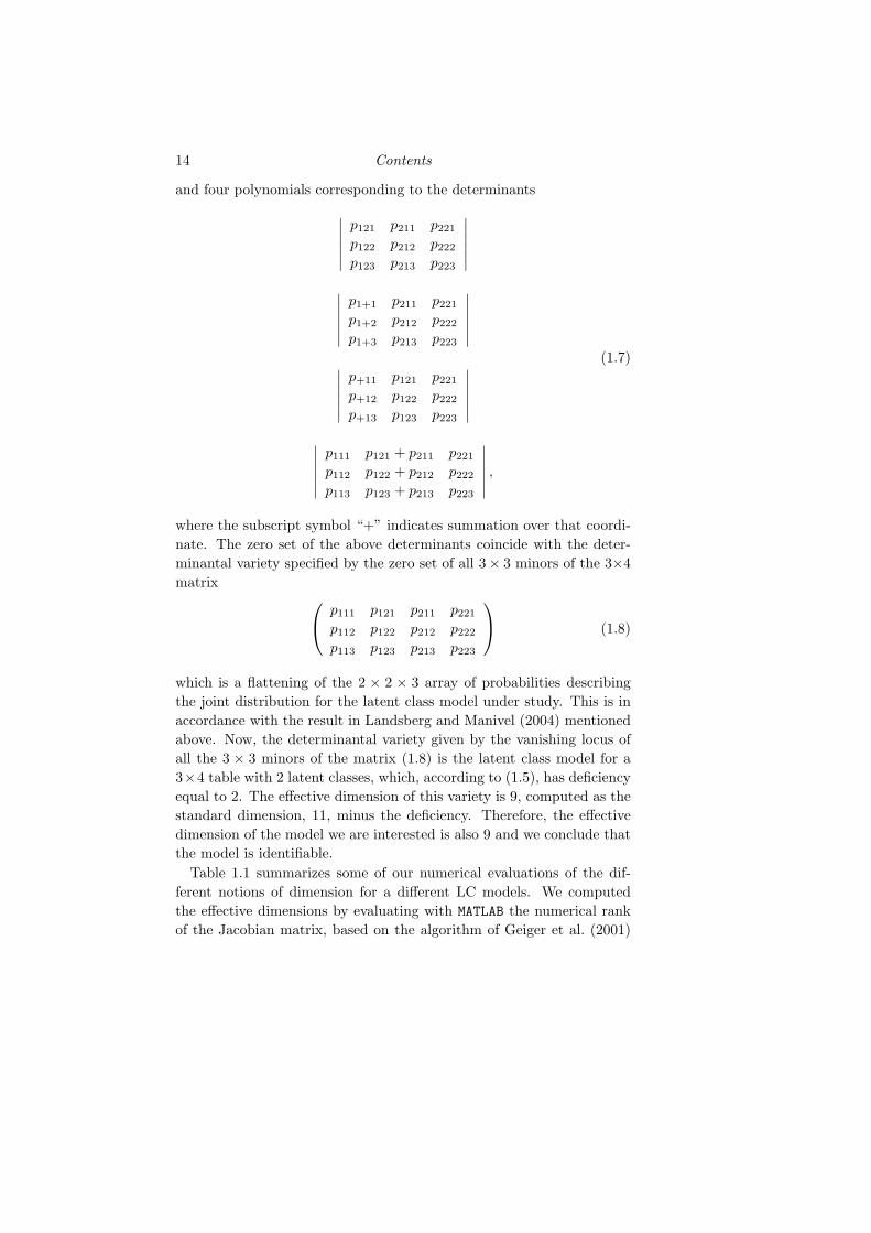
14 Contents

and four polynomials corresponding to the determinants∣∣∣∣∣∣p121 p211 p221

p122 p212 p222

p123 p213 p223

∣∣∣∣∣∣∣∣∣∣∣∣p1+1 p211 p221

p1+2 p212 p222

p1+3 p213 p223

∣∣∣∣∣∣∣∣∣∣∣∣p+11 p121 p221

p+12 p122 p222

p+13 p123 p223

∣∣∣∣∣∣∣∣∣∣∣∣p111 p121 + p211 p221

p112 p122 + p212 p222

p113 p123 + p213 p223

∣∣∣∣∣∣ ,

(1.7)

where the subscript symbol “+” indicates summation over that coordi-nate. The zero set of the above determinants coincide with the deter-minantal variety specified by the zero set of all 3× 3 minors of the 3×4matrix p111 p121 p211 p221

p112 p122 p212 p222

p113 p123 p213 p223

(1.8)

which is a flattening of the 2 × 2 × 3 array of probabilities describingthe joint distribution for the latent class model under study. This is inaccordance with the result in Landsberg and Manivel (2004) mentionedabove. Now, the determinantal variety given by the vanishing locus ofall the 3 × 3 minors of the matrix (1.8) is the latent class model for a3×4 table with 2 latent classes, which, according to (1.5), has deficiencyequal to 2. The effective dimension of this variety is 9, computed as thestandard dimension, 11, minus the deficiency. Therefore, the effectivedimension of the model we are interested is also 9 and we conclude thatthe model is identifiable.

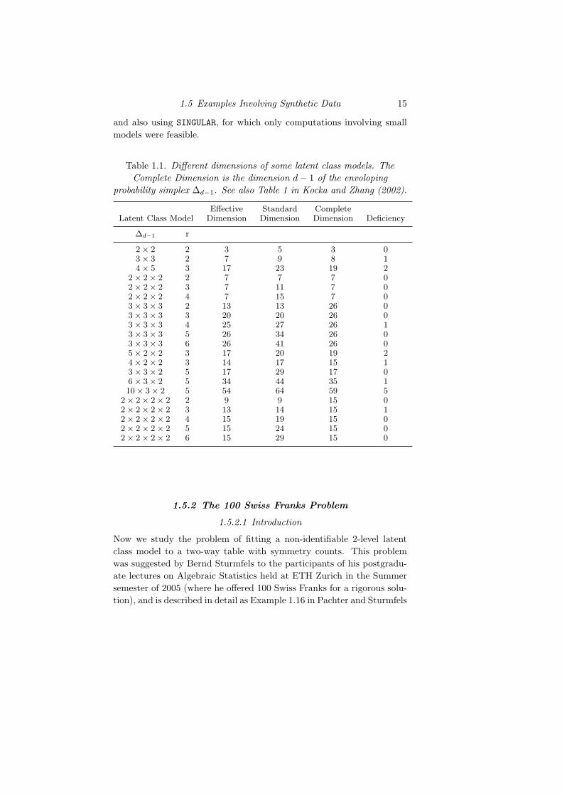
Table 1.1 summarizes some of our numerical evaluations of the dif-ferent notions of dimension for a different LC models. We computedthe effective dimensions by evaluating with MATLAB the numerical rankof the Jacobian matrix, based on the algorithm of Geiger et al. (2001)


and also using SINGULAR, for which only computations involving smallmodels were feasible.

Table 1.1. Different dimensions of some latent class models. TheComplete Dimension is the dimension d− 1 of the envoloping

probability simplex ∆d−1. See also Table 1 in Kocka and Zhang (2002).

Effective Standard CompleteLatent Class Model Dimension Dimension Dimension Deficiency

∆d−1 r

2× 2 2 3 5 3 03× 3 2 7 9 8 14× 5 3 17 23 19 2

2 × 2 × 2 2 7 7 7 02 × 2 × 2 3 7 11 7 02 × 2 × 2 4 7 15 7 03 × 3 × 3 2 13 13 26 03 × 3 × 3 3 20 20 26 03 × 3 × 3 4 25 27 26 13 × 3 × 3 5 26 34 26 03 × 3 × 3 6 26 41 26 05 × 2 × 2 3 17 20 19 24 × 2 × 2 3 14 17 15 13 × 3 × 2 5 17 29 17 06 × 3 × 2 5 34 44 35 110 × 3 × 2 5 54 64 59 5

2× 2× 2× 2 2 9 9 15 02× 2× 2× 2 3 13 14 15 12× 2× 2× 2 4 15 19 15 02× 2× 2× 2 5 15 24 15 02× 2× 2× 2 6 15 29 15 0

1.5.2 The 100 Swiss Franks Problem

1.5.2.1 Introduction

Now we study the problem of fitting a non-identifiable 2-level latentclass model to a two-way table with symmetry counts. This problemwas suggested by Bernd Sturmfels to the participants of his postgradu-ate lectures on Algebraic Statistics held at ETH Zurich in the Summersemester of 2005 (where he offered 100 Swiss Franks for a rigorous solu-tion), and is described in detail as Example 1.16 in Pachter and Sturmfels

16 Contents

(2005). The observed table is

n =

4 2 2 22 4 2 22 2 4 22 2 2 4

(1.9)

and the 100 Swiss Franks problem requires proving that the three tablesin Table 1.2 a) are local maxima for the the basic LC model with onebinary latent variable. For this model, the standard dimension of Θ =∆3×∆3×∆1 is 2(3+3)+1 = 13 and, by (1.5), the deficiency is 2. Thus,the model is not identifiable and the pre-image of each point p ∈ H bythe map (1.6) is a 2-dimensional surface in Θ. To keep the notationlight, we write αih for p(h)

1 (i) and βjh for p(h)2 (j), where i, j = 1, . . . , 4

and α(h) and β(h) for the conditional marginal distribution of X1 andX2 given H = h, respectively. The accounting equations for the pointsin H become

pij =∑

h∈{1,2}

λhαihβjh, i, j ∈ [4] (1.10)

and the log-likelihood function, ignoring an irrelevant additive constant,is

`(θ) =∑i,j

nij log

∑h∈{1,2}

λhαihβjh

, θ ∈ ∆3 ×∆3 ×∆1.

It is worth emphasizing, as we did above and as the previous displayclearly shows, that the observed counts are minimal sufficient statistics.

Alternatively, we can re-parametrize the log-likelihood function usingdirectly the points in H rather than the points in the parameter spaceΘ. Recall from our discussion in section 1.4 that, for this model, the4× 4 array p is in H if and only if each 3× 3 minor vanishes. Then, wecan write the log-likelihood function as

`(p) =∑i,j

nij log pij , p ∈ ∆15, det(p∗ij) = 0 all i, j ∈ [4], (1.11)

where p∗ij is the 3 × 3 sub-matrix of p obtained by erasing the ith rowand the jth column.

Although the first order optimality conditions for the Lagrangian cor-responding to the parametrization (1.11) are algebraically simpler andcan be given the form of a system of polynomial equations, in prac-tice, the classical parametrization (1.10) is used in both the EM and


the Newton-Raphson implementations in order to compute the maxi-mum likelihood estimate of p. See Goodman (1979), Haberman (1988),and Redner and Walker (1984) for more details about these numericalprocedures.

1.5.2.2 Global and Local Maxima

Using both the EM and Newton-Raphson algorithm with several dif-ferent starting points, we found 7 local maxima of the log-likelihoodfunction, reported in Table 1.2. The maximal value was found exper-imentally to be −20.8074 + const., where const. denotes the additiveconstant stemming from the multinomial coefficient. The maximum isachieved by the three tables of fitted values Table 1.2 a). The remain-ing four tables are local maxima of −20.8616 + const., close in value tothe actual global maximum. Using SINGULAR (see (Greuel et al., 2005)),we checked that the tables found satisfy the first order optimality con-ditions (1.11). After verifying numerically the second order optimalityconditions, we conclude that those points are indeed local maxima. Asnoted in Pachter and Sturmfels (2005), the log-likelihood function alsohas a few saddle points.

A striking feature of the global maxima in Table 1.2 is their invari-ance under the action of the symmetric group on four elements actingsimultaneously on the row and columns. Different symmetries arise forthe local maxima. We will give an explicit representation of these sym-metries under the classical parametrization (1.10) in the next section.

Despite the simplicity and low-dimensionality of the LC model forthis table and the strong symmetric features of the data, we have yetto provide a purely mathematical proof that the three top arrays inTable 1.2 correspond to a global maximum of the likelihood function.We view the difficulty and complexity of the 100 Swiss Franks problemas a consequence of the inherent difficulty of even small LC modelsand perhaps an indication that the current theory has still many open,unanswered problems. In Section 1.7, we present partial results towardsthe completion of the proof.

1.5.2.3 Unidentifiable Space

It follows from equation (1.5) that the non-identifiable subspaces are atwo-dimensional subsets of Θ. We give an explicit algebraic descriptionof this space, which we will then use to obtain interpretable plots of theprofile likelihood.

Firstly, we focus on the three global maxima in Table 1.2 a). By

18 Contents

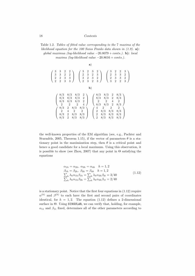
Table 1.2. Tables of fitted value corresponding to the 7 maxima of thelikelihood equation for the 100 Swiss Franks data shown in (1.9). a):

global maximua (log-likelihood value −20.8079 + conts.). b): localmaxima (log-likelihood value −20.8616 + conts.).

a)0B@ 3 3 2 23 3 2 22 2 3 32 2 3 3

1CA0B@ 3 2 3 2

2 3 2 33 2 3 22 3 2 3

1CA0B@ 3 2 2 3

2 3 3 22 3 3 23 2 2 3

1CAb)0B@ 8/3 8/3 8/3 2

8/3 8/3 8/3 28/3 8/3 8/3 22 2 2 4

1CA0B@ 8/3 8/3 2 8/3

8/3 8/3 2 8/32 2 4 2

8/3 8/3 2 8/3

1CA0B@ 8/3 2 8/3 8/3

2 4 2 28/3 2 8/3 8/38/3 2 8/3 8/3

1CA0B@ 4 2 2 2

2 8/3 8/3 8/32 8/3 8/3 8/32 8/3 8/3 8/3

1CA

the well-known properties of the EM algorithm (see, e.g., Pachter andSturmfels, 2005, Theorem 1.15), if the vector of parameters θ is a sta-tionary point in the maximization step, then θ is a critical point andhence a good candidate for a local maximum. Using this observation, itis possible to show (see Zhou, 2007) that any point in Θ satisfying theequations

α1h = α2h, α3h = α4h h = 1, 2β1h = β2h, β3h = β4h h = 1, 2∑h λhα1hβ1h =

∑h λhα3hβ3t = 3/40∑

h λhα1hβ3h =∑h λhα3hβ1t = 2/40

(1.12)

is a stationary point. Notice that the first four equations in (1.12) requireα(h) and β(h) to each have the first and second pairs of coordinatesidentical, for h = 1, 2. The equation (1.12) defines a 2-dimensionalsurface in Θ. Using SINGULAR, we can verify that, holding, for example,α11 and β11 fixed, determines all of the other parameters according to


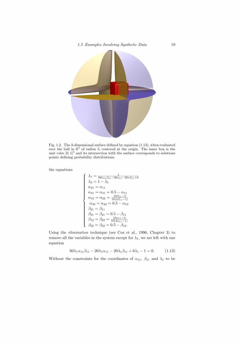
Fig. 1.2. The 2-dimensional surface defined by equation (1.13), when evaluatedover the ball in R3 of radius 3, centered at the origin. The inner box is theunit cube [0, 1]3 and its intersection with the surface corresponds to solutionspoints defining probability distributions.

the equations

λ1 = 180α11β11−20α11−20∗β11+6

λ2 = 1− λ1

α21 = α11

α31 = α41 = 0.5− α11

α12 = α22 = 10β11−310(4β11−1)

α32 = α42 = 0.5− α12

β21 = β11

β31 = β41 = 0.5− β11

β12 = β22 = 10α11−310(4α11−1)

β32 = β42 = 0.5− β12.

Using the elimination technique (see Cox et al., 1996, Chapter 3) toremove all the variables in the system except for λ1, we are left with oneequation

80λ1α11β11 − 20λ1α11 − 20λ1β11 + 6λ1 − 1 = 0. (1.13)

Without the constraints for the coordinates of α11, β11 and λ1 to be

20 Contents

probabilities, (1.13) defines a two-dimensional surface in R3, depicted inFigure 1.2. Notice that the axes do not intersect this surface, so that zerois not a possible value for α11, β11 and λ1. Because the non-identifiablespace in Θ is 2-dimensional, equation (1.13) actually defines a bijectionbetween α11, β11 and λ1 and the rest of the parameters. Then, theintersection of the surface (1.13) with the unit cube [0, 1]3, depicted as ared box in Figure 1.2, is the projection of the non-identifiable subspaceinto the 3-dimensional unit cube where α11, β11 and λ1 live. Figure 1.3displays two different views of this projection.

The preceding arguments hold unchanged if we replace the symme-try conditions in the first two lines of equation (1.12) with either ofthese other two conditions, requiring different pairs of coordinates to beidentical, namely

α1h = α3h, α2h = α4h, β1h = β3h, β2h = β4h (1.14)

and

α1h = α4h, α2h = α3h, β1h = β4h, β2h = β3h, (1.15)

where h = 1, 2.The non-identifiable surfaces inside Θ corresponding each to one of

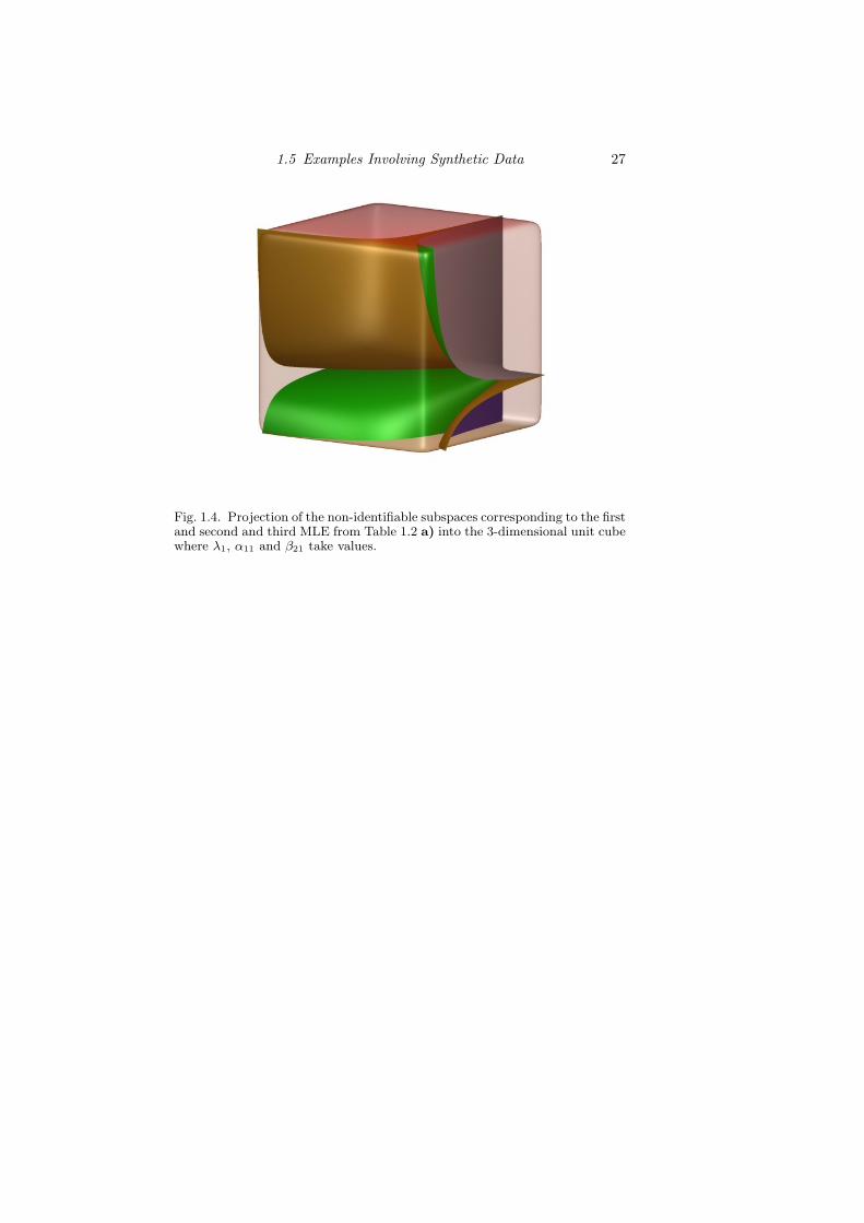
the three pairs of coordinates held fixed in equations (1.12), (1.14) and(1.15), produce the three distinct tables of maximum likelihood esti-mates reported in Table 1.2 a). Figure 1.3 shows the projection of thenon-identifiable subspaces for the three MLEs in Table 1.2 a) into thethree dimensional unit cube for λ1, α11 and β11. Although each of thesethree subspaces are disjoint subsets of Θ, their lower dimensional projec-tions comes out as unique. By projecting onto the different coordinatesλ1, α11 and β21 instead, we obtain two disjoint surfaces for the first, andsecond and third MLE, shown in Figure 1.4.

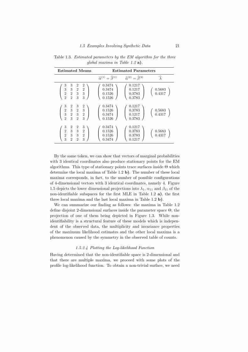
Table 1.3 presents some estimated parameters using the EM algo-rithm. Though these estimates are hardly meaningful, because of thenon-identifiability issue, they show the symmetry properties we pointedout above and implicit in equations (1.12), (1.14) and (1.15), and theyexplain the invariance under simultaneous permutation of the fitted ta-bles. In fact, the number of global maxima is the number of differentconfigurations of the 4 dimensional vectors of estimated marginal prob-abilities with two identical coordinates, namely 3. This phenomenon,entirely due to the strong symmetry in the observed table (1.9), is com-pletely separate from the non-identrifiability issues, but just as problem-atic.


Table 1.3. Estimated parameters by the EM algorithm for the threeglobal maxima in Table 1.2 a).

Estimated Means Estimated Parameters

bα(1) = bβ(1) bα(2) = bβ(2) bλ0B@ 3 3 2 23 3 2 22 2 3 32 2 3 3

1CA0B@ 0.3474

0.34740.15260.1526

1CA0B@ 0.1217

0.12170.37830.3783

1CA „0.56830.4317

«0B@ 3 2 3 2

2 3 2 33 2 3 22 3 2 3

1CA0B@ 0.3474

0.15260.34740.1526

1CA0B@ 0.1217

0.37830.12170.3783

1CA „0.56830.4317

«0B@ 3 2 2 3

2 3 3 22 3 3 23 2 2 3

1CA0B@ 0.3474

0.15260.15260.3474

1CA0B@ 0.1217

0.37830.37830.1217

1CA „0.56830.4317

«

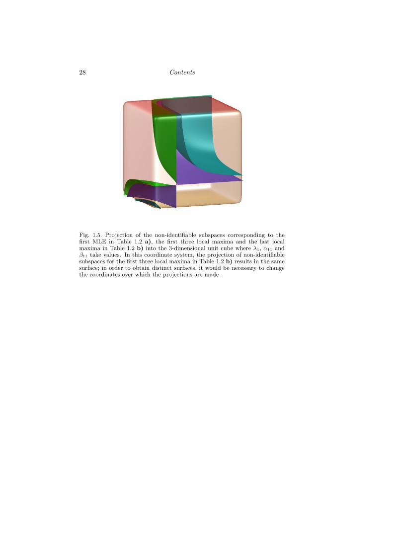
By the same token, we can show that vectors of marginal probabilitieswith 3 identical coordinates also produce stationary points for the EMalgorithms. This type of stationary points trace surfaces inside Θ whichdetermine the local maxima of Table 1.2 b). The number of these localmaxima corresponds, in fact, to the number of possible configurationsof 4-dimensional vectors with 3 identical coordinates, namely 4. Figure1.5 depicts the lower dimensional projections into λ1, α11 and β11 of thenon-identifiable subspaces for the first MLE in Table 1.2 a), the firstthree local maxima and the last local maxima in Table 1.2 b).

We can summarize our finding as follows: the maxima in Table 1.2define disjoint 2-dimensional surfaces inside the parameter space Θ, theprojection of one of them being depicted in Figure 1.3. While non-identifiability is a structural feature of these models which is indepen-dent of the observed data, the multiplicity and invariance propertiesof the maximum likelihood estimates and the other local maxima is aphenomenon caused by the symmetry in the observed table of counts.

1.5.2.4 Plotting the Log-likelihood Function

Having determined that the non-identifiable space is 2-dimensional andthat there are multiple maxima, we proceed with some plots of theprofile log-likelihood function. To obtain a non-trivial surface, we need

22 Contents

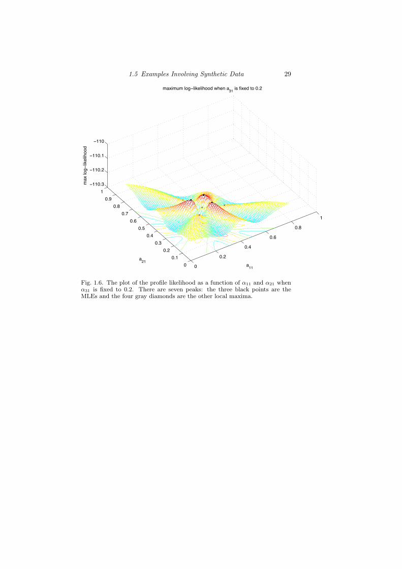
to consider three parameters. Figures 1.9 and 1.7 display the surfaceand contour plot respectively of the profile log-likelihhod function forα11 and α21 when α31 is one of the fixed parameters. Both Figures showclearly the different maxima, each lying on the top of “ridges” of thelog-likelihood surface which are placed symmetrically with respect toeach others. The position and shapes of these ridges reflect, once again,the symmetric properties of the estimated probabilities and parameters.

1.5.2.5 Further Remarks and Open Problem

We conclude this section with some observations and pointers to openproblems.

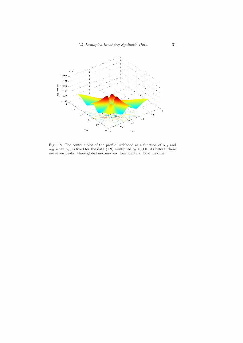
One of the interesting aspects we came across while fitting the table(1.9) was the proximity of the values of the local and global maximaof the log-likelihood function. Furthermore, although these values arevery close, the fitted tables corresponding to global and local maximaare remarkably different. Even though the data (1.9) are not sparse, wewonder about the effect of cell sizes. Figure 1.8 show the same profilelog-likelihood for the table (1.9) multiplied by 10,000. While the numberof global and local maxima, the contour plot and the basic symmetricshape of the profile log-likelihood surface remain unchanged after thisrescaling, the peaks around the global maxima have become much morepronounced and so has the difference between of the values of the globaland local maxima.

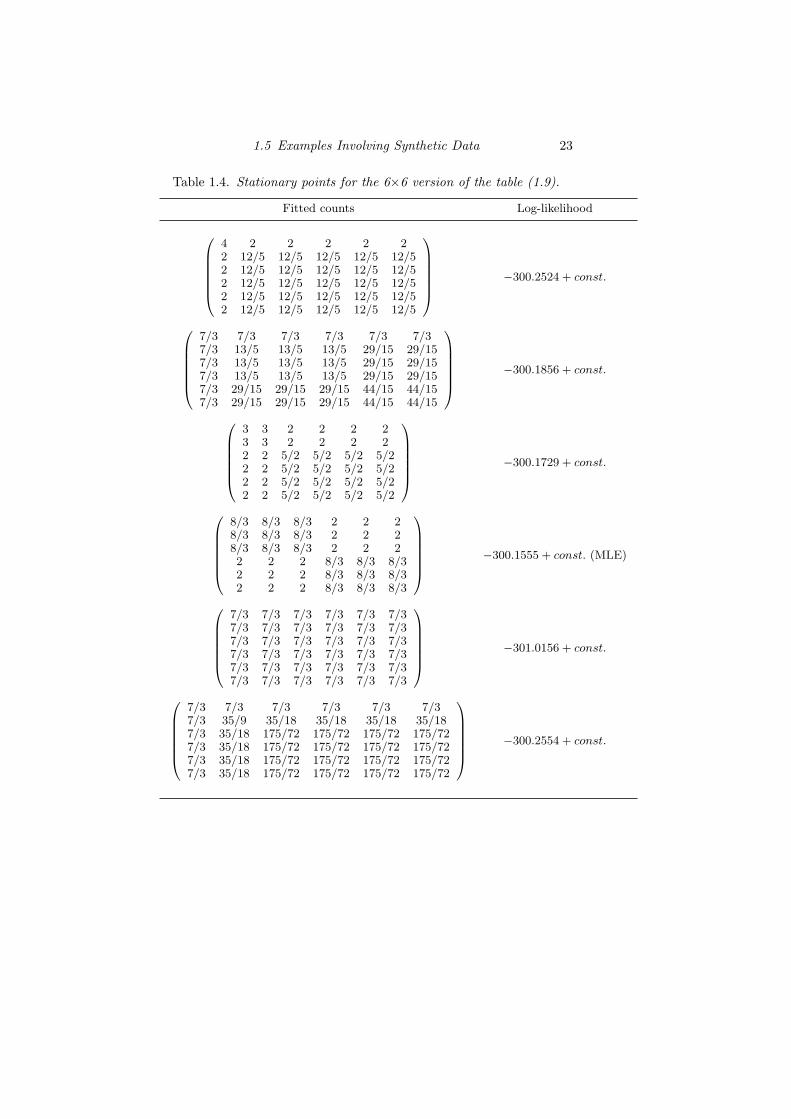
We have looked at a number of variations of table (1.9), focussing inparticular on the symmetric data. We report only some of our resultsand refer to Zhou (2007) for a more extensive study. Table 1.4 shows thevalues and number of local and global maxima for a the 6× 6 version of(1.9). As for the 4× 4 case, we notice strong invariance features of thevarious maxima of the likelihood function and a very small differencebetween the value of the global and local maxima.

Fitting the same model to the table1 2 2 22 1 2 22 2 1 22 2 2 1

we found 6 global maxima of the likelihood function (their value was−77.2927 + const.), which give as many maximum likelihood estimates,all obtainable via simultaneous permutation of rows and columns of the


Table 1.4. Stationary points for the 6×6 version of the table (1.9).

Fitted counts Log-likelihood

0BBBBB@4 2 2 2 2 22 12/5 12/5 12/5 12/5 12/52 12/5 12/5 12/5 12/5 12/52 12/5 12/5 12/5 12/5 12/52 12/5 12/5 12/5 12/5 12/52 12/5 12/5 12/5 12/5 12/5

1CCCCCA −300.2524 + const.

0BBBBB@7/3 7/3 7/3 7/3 7/3 7/37/3 13/5 13/5 13/5 29/15 29/157/3 13/5 13/5 13/5 29/15 29/157/3 13/5 13/5 13/5 29/15 29/157/3 29/15 29/15 29/15 44/15 44/157/3 29/15 29/15 29/15 44/15 44/15


0BBBBB@3 3 2 2 2 23 3 2 2 2 22 2 5/2 5/2 5/2 5/22 2 5/2 5/2 5/2 5/22 2 5/2 5/2 5/2 5/22 2 5/2 5/2 5/2 5/2


0BBBBB@8/3 8/3 8/3 2 2 28/3 8/3 8/3 2 2 28/3 8/3 8/3 2 2 22 2 2 8/3 8/3 8/32 2 2 8/3 8/3 8/32 2 2 8/3 8/3 8/3

1CCCCCA −300.1555 + const. (MLE)

0BBBBB@7/3 7/3 7/3 7/3 7/3 7/37/3 7/3 7/3 7/3 7/3 7/37/3 7/3 7/3 7/3 7/3 7/37/3 7/3 7/3 7/3 7/3 7/37/3 7/3 7/3 7/3 7/3 7/37/3 7/3 7/3 7/3 7/3 7/3


0BBBBB@7/3 7/3 7/3 7/3 7/3 7/37/3 35/9 35/18 35/18 35/18 35/187/3 35/18 175/72 175/72 175/72 175/727/3 35/18 175/72 175/72 175/72 175/727/3 35/18 175/72 175/72 175/72 175/727/3 35/18 175/72 175/72 175/72 175/72


24 Contents

table 7/4 7/4 7/4 7/47/4 7/4 7/4 7/47/4 7/4 7/6 7/37/4 7/4 7/3 7/6

.

Based on the various cases we have investigated, we have the followingconjecture, which we verified computationally up to dimension k = 50:

Conjecture: The MLEs For the n × n table with values x along thediagonal and values y ≤ x for off the diagonal elements, the maximumlikelihood estimates for the latent class model with 2 latent classes are

the 2×2 block diagonal matrix of the form(

A B

B′ C

)and the permu-

tated versions of it, where A, B, and C are

A =(y + x−y

p

)· 1p×p,

B = y · 1p×q,C =

(y + x−y

q

)· 1q×q,

and p =⌊n2

⌋, q = n− p.

We also noticed other interesting phenomena, which suggest the needfor further geometric analysis. For example, consider fitting the (non-identifiable) latent class model with 2 levels to the table of counts (sug-gested by Bernd Sturmfels) 5 1 1

1 6 21 2 6

.

Based on our computations, the maximum likelihood estimates appearto be unique, namely the table of fitted values 5 1 1

1 4 41 4 4

. (1.16)

Looking at the non-identifiable subspace for this model, we foundthat the MLEs (1.16) can arise from combinations of parameters someof which can be 0, such as

α(1) = β(1) =

0.71430.14290.1429

, α(2) = β(2) =

00.50.5

, λ =(

0.39200.6080

).


This finding seems to indicate the possibility of singularities besides theobvious ones given by marginal probabilities for H containing 0 coor-dinates (which have the geometric interpretation as lower order secantvarieties) and by points p along the boundary of the simplex ∆d−1.

26 Contents

Fig. 1.3. Intersection of the surface defined by equation (1.13) with the unitcube [0, 1]3, from two different views.


Fig. 1.4. Projection of the non-identifiable subspaces corresponding to the firstand second and third MLE from Table 1.2 a) into the 3-dimensional unit cubewhere λ1, α11 and β21 take values.

28 Contents

Fig. 1.5. Projection of the non-identifiable subspaces corresponding to thefirst MLE in Table 1.2 a), the first three local maxima and the last localmaxima in Table 1.2 b) into the 3-dimensional unit cube where λ1, α11 andβ11 take values. In this coordinate system, the projection of non-identifiablesubspaces for the first three local maxima in Table 1.2 b) results in the samesurface; in order to obtain distinct surfaces, it would be necessary to changethe coordinates over which the projections are made.


0

0.2

0.4

0.6

0.8

1

00.1

0.20.3

0.40.5

0.60.7

0.80.9

1!110.3

!110.2

!110.1

!110

a11

maximum log!likelihood when a31 is fixed to 0.2

a21

max

log!

likel

ihoo

d

Fig. 1.6. The plot of the profile likelihood as a function of α11 and α21 whenα31 is fixed to 0.2. There are seven peaks: the three black points are theMLEs and the four gray diamonds are the other local maxima.

30 Contents

0 0.1 0.2 0.3 0.4 0.5 0.6 0.7 0.8 0.90

0.1

0.2

0.3

0.4

0.5

0.6

0.7

0.8

0.9

a11

a 21

maximum log!likelihood when a31 is fixed to 0.2

Fig. 1.7. The contour plot of the profile likelihood as a function of α11 andα21 when α31 is fixed. There are seven peaks: the three black points are theMLEs and the four gray points are the other local maxima.


Fig. 1.8. The contour plot of the profile likelihood as a function of α11 andα21 when α31 is fixed for the data (1.9) multiplied by 10000. As before, thereare seven peaks: three global maxima and four identical local maxima.

32 Contents

1.6 Two Applications

1.6.1 Example: Michigan Influenza

Monto et al. (1985) present data for 263 individuals on the outbreakof influenza in Tecumseh, Michigan during the four winters of 1977-1981: (1) Influenza type A (H3N2), December 1977–March 1978; (2)Influenza type A (H1N1), January 1979–March 1979; (3) Influenza typeB, January 1980–April 1980 and (4) Influenza type A (H3N2), December1980–March 1981. The data have been analyzed by others includingHaber (1986) and we reproduce them here as Table 1.5. This tableis characterized by a large count for the cell corresponding to lack ofinfection from any type of influenza.

Table 1.5. Infection profiles and frequency of infection for fourinfluenza outbreaks for a sample of 263 individuals in Tecumseh,

Michigan during the winters of 1977-1981. A value of 0 in the first fourcolumns codes the lack of infection. Source: Monto et al. (1985). The

last column is the values fitted by the naive Bayes model with r = 2.

Type of Influenza Observed Counts Fitted Values

(1) (2) (3) (4)

0 0 0 0 140 139.51350 0 0 1 31 31.32130 0 1 0 16 16.63160 0 1 1 3 2.71680 1 0 0 17 17.15820 1 0 1 2 2.11220 1 1 0 5 5.11720 1 1 1 1 0.42921 0 0 0 20 20.81601 0 0 1 2 1.69751 0 1 0 9 7.73541 0 1 1 0 0.56791 1 0 0 12 11.54721 1 0 1 1 0.83411 1 1 0 4 4.48091 1 1 1 0 0.3209

The LC model with one binary latent variable (which is identifiableby Theorem 3.5 in Settimi and Smith, 2005) fits the data extremely well,as shown in Table 1.5. We also conducted a log-linear model analysis ofthis dataset and concluded that there is no indication of second or higherorder interaction among the four types of influenza. The best log-linear

1.6 Two Applications 33

model selected via both Pearson’s chi-squared and the likelihood ratiostatistic was the model of conditional independence of influenza of type(2), (3) and (4) given influenza of type (1) and was outperformed by theLC model.

Despite the reduced dimensionality of this problem and the large sam-ple size, we report on the instability of the Fisher scoring algorithmimplemented in the R package gllm, e.g., see Espeland (1986). As thealgorithm cycles through, the evaluations of the expected Fisher infor-mation matrix become increasing ill-conditioned and eventually produceinstabilities in the estimated coefficients and, in particular, in the stan-dard errors. These problems disappear in the modified Newton-Raphsonimplementation, originally suggested by Haberman (1988), based on aninexact line search method known in the convex optimization literatureas the Wolfe condition.

1.6.2 Data From the National Long Term Care Survey

Erosheva (2002) and Erosheva et al. (2007) analyze an extract from theNational Long Term Care Survey in the form of a 216 contingency tablethat contains data on 6 activities of daily living (ADL) and 10 instru-mental activities of daily living (IADL) for community-dwelling elderlyfrom 1982, 1984, 1989, and 1994 survey waves. The 6 ADL items includebasic activities of hygiene and personal care (eating, getting in/out ofbed, getting around inside, dressing, bathing, and getting to the bath-room or using toilet). The 10 IADL items include basic activities nec-essary to reside in the community (doing heavy housework, doing lighthousework, doing laundry, cooking, grocery shopping, getting about out-side, travelling, managing money, taking medicine, and telephoning). Ofthe 65,536 cells in the table, 62,384 (95.19%) contain zero counts, 1,729(2.64%)contain counts of 1, 499 (0.76%) contain counts of 2. The largestcell count, corresponding to the (1, 1, . . . , 1) cell, is 3,853.

Erosheva (2002) and Erosheva et al. (2007) use an individual-levellatent mixture model that bears a striking resemblance to the LC model.Here we report on analyses with the latter.

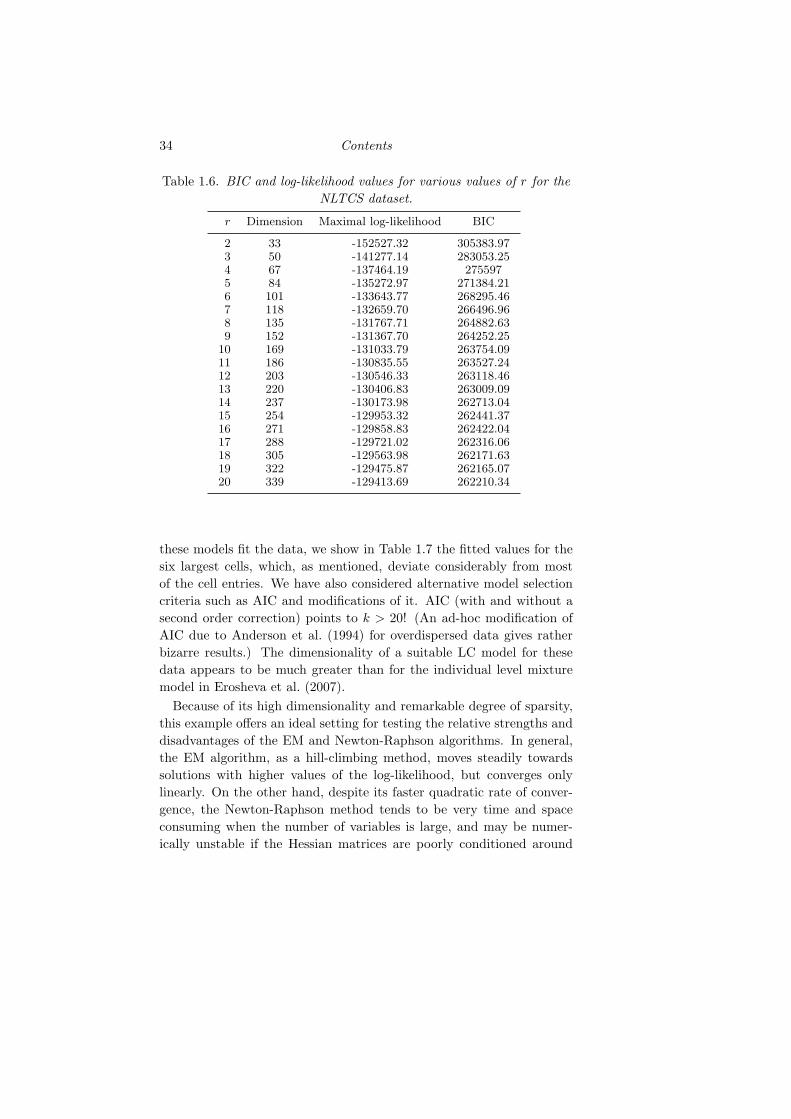
We use both the EM and Newton-Raphson algorithms to fit a numberof LC models with up to 20 classes, which can be shown to be all iden-tifiable in virtue of Proposition 2.3 in Catalisano et al. (2002). Table1.6 reports the maximal values of the log-likelihood function and thevalues of the BIC, which seem to indicate that larger LC models withmany levels are to be preferred. To provide a better sense of how well

34 Contents

Table 1.6. BIC and log-likelihood values for various values of r for theNLTCS dataset.

r Dimension Maximal log-likelihood BIC

2 33 -152527.32 305383.973 50 -141277.14 283053.254 67 -137464.19 2755975 84 -135272.97 271384.216 101 -133643.77 268295.467 118 -132659.70 266496.968 135 -131767.71 264882.639 152 -131367.70 264252.25

10 169 -131033.79 263754.0911 186 -130835.55 263527.2412 203 -130546.33 263118.4613 220 -130406.83 263009.0914 237 -130173.98 262713.0415 254 -129953.32 262441.3716 271 -129858.83 262422.0417 288 -129721.02 262316.0618 305 -129563.98 262171.6319 322 -129475.87 262165.0720 339 -129413.69 262210.34

these models fit the data, we show in Table 1.7 the fitted values for thesix largest cells, which, as mentioned, deviate considerably from mostof the cell entries. We have also considered alternative model selectioncriteria such as AIC and modifications of it. AIC (with and without asecond order correction) points to k > 20! (An ad-hoc modification ofAIC due to Anderson et al. (1994) for overdispersed data gives ratherbizarre results.) The dimensionality of a suitable LC model for thesedata appears to be much greater than for the individual level mixturemodel in Erosheva et al. (2007).

Because of its high dimensionality and remarkable degree of sparsity,this example offers an ideal setting for testing the relative strengths anddisadvantages of the EM and Newton-Raphson algorithms. In general,the EM algorithm, as a hill-climbing method, moves steadily towardssolutions with higher values of the log-likelihood, but converges onlylinearly. On the other hand, despite its faster quadratic rate of conver-gence, the Newton-Raphson method tends to be very time and spaceconsuming when the number of variables is large, and may be numer-ically unstable if the Hessian matrices are poorly conditioned around

1.6 Two Applications 35

Table 1.7. Fitted values for the largest six cells for the NLTCS datasetfor various values of r.

r Fitted values

2 826.78 872.07 6.7 506.61 534.36 237.413 2760.93 1395.32 152.85 691.59 358.95 363.184 2839.46 1426.07 145.13 688.54 350.58 383.195 3303.09 1436.95 341.67 422.24 240.66 337.636 3585.98 1294.25 327.67 425.37 221.55 324.717 3659.80 1258.53 498.76 404.57 224.22 299.528 3663.02 1226.81 497.59 411.82 227.92 291.999 3671.29 1221.61 526.63 395.08 236.95 294.54

10 3665.49 1233.16 544.95 390.92 237.69 297.7211 3659.20 1242.27 542.72 393.12 244.37 299.2612 3764.62 1161.53 615.99 384.81 235.32 260.0413 3801.73 1116.40 564.11 374.97 261.83 240.6414 3796.38 1163.62 590.33 387.73 219.89 220.3415 3831.09 1135.39 660.46 361.30 261.92 210.3116 3813.80 1145.54 589.27 370.48 245.92 219.0617 3816.45 1145.45 626.85 372.89 236.16 213.2518 3799.62 1164.10 641.02 387.98 219.65 221.7719 3822.68 1138.24 655.40 365.49 246.28 213.4420 3836.01 1111.51 646.39 360.52 285.27 220.47

Observed 3853 1107 660 351 303 216

critical points, which again occurs more frequently in large problems(but also in small ones, such as the Michigan Influenza examples above).

For the class of basic LC models considered in this paper, the timecomplexity for one single step of the EM algorithm is O (d · r ·

∑i di),

while the space complexity is O (d · r). In contrast, for the Newton-Raphson algorithm, both the time and space complexity areO

(d · r2 ·

∑i di).

Consequently, for the NLTCS dataset, when r is bigger than 4, Newton-Raphson is sensibly slower than EM, and when r goes up to 7, Newton-Raphson needs more than 1G of memory. Another significant drawbackof the Newton-Raphson method we experienced while fitting both theMichigan influenza and the NLTCS dataset is its potential numerical in-stability, due to the large condition numbers of the Hessian matrices. Asremarked at the end of the previous section, following Haberman (1988),a numerically convenient solution is to modify the Hessian matrices sothat they remain negative definite and then approximate locally the log-likelihood by a quadratic function. However, since the log-likelihood isneither concave nor quadratic, these modifications do not necessarily

36 Contents

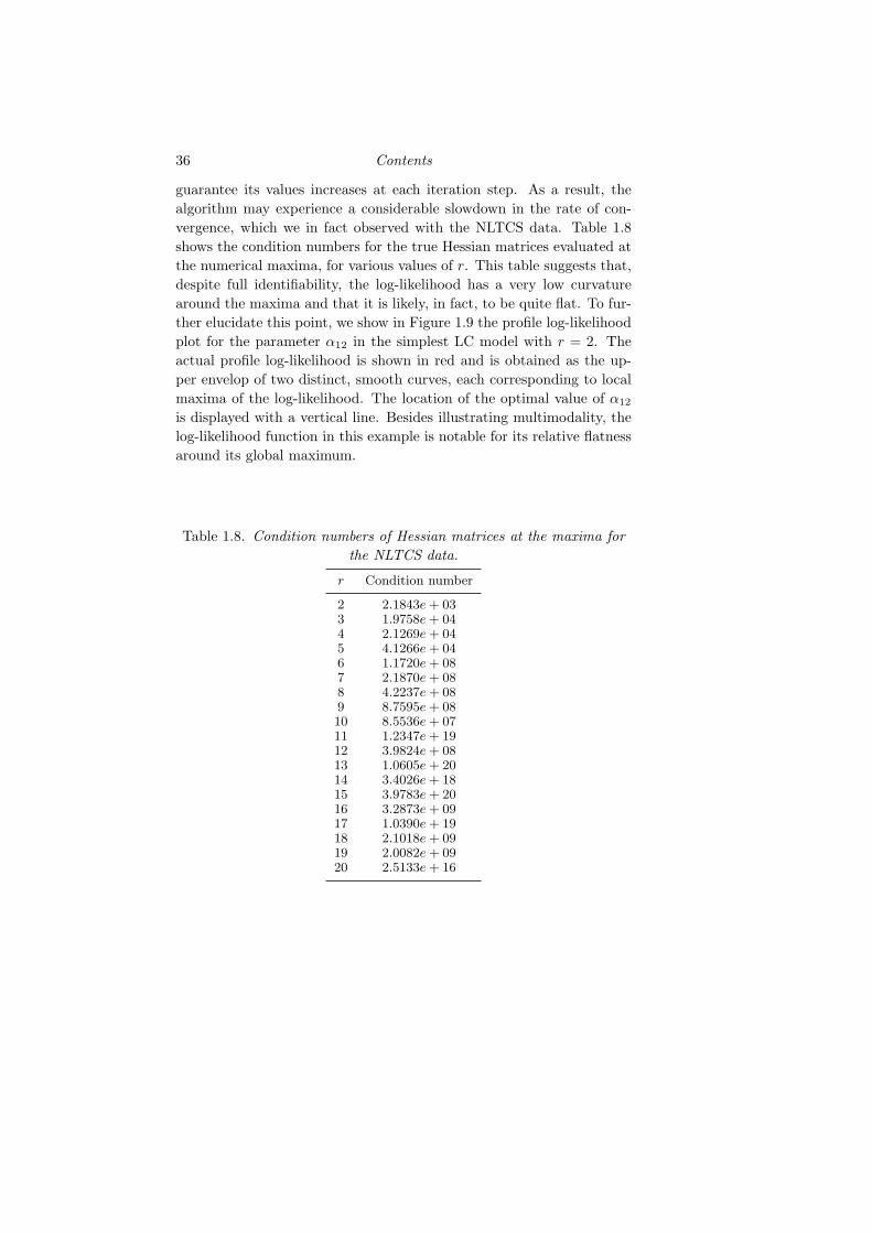
guarantee its values increases at each iteration step. As a result, thealgorithm may experience a considerable slowdown in the rate of con-vergence, which we in fact observed with the NLTCS data. Table 1.8shows the condition numbers for the true Hessian matrices evaluated atthe numerical maxima, for various values of r. This table suggests that,despite full identifiability, the log-likelihood has a very low curvaturearound the maxima and that it is likely, in fact, to be quite flat. To fur-ther elucidate this point, we show in Figure 1.9 the profile log-likelihoodplot for the parameter α12 in the simplest LC model with r = 2. Theactual profile log-likelihood is shown in red and is obtained as the up-per envelop of two distinct, smooth curves, each corresponding to localmaxima of the log-likelihood. The location of the optimal value of α12

is displayed with a vertical line. Besides illustrating multimodality, thelog-likelihood function in this example is notable for its relative flatnessaround its global maximum.

Table 1.8. Condition numbers of Hessian matrices at the maxima forthe NLTCS data.

r Condition number

2 2.1843e+ 033 1.9758e+ 044 2.1269e+ 045 4.1266e+ 046 1.1720e+ 087 2.1870e+ 088 4.2237e+ 089 8.7595e+ 0810 8.5536e+ 0711 1.2347e+ 1912 3.9824e+ 0813 1.0605e+ 2014 3.4026e+ 1815 3.9783e+ 2016 3.2873e+ 0917 1.0390e+ 1918 2.1018e+ 0919 2.0082e+ 0920 2.5133e+ 16

1.7 On Symmetric Tables and the MLE 37

Fig. 1.9. The plot of the profile likelihood for the NLCST dataset, as a functionof α12. The vertical line indicates the location of the maximizer.

1.7 On Symmetric Tables and the MLE

In this section, inspired by the 100 Swiss Franks problem (1.9), we in-vestigate in detail some of the effects that invariance to row and columnpermutations of the observed table have on the MLE. In particular, westudy the seemingly simple problem of computing the MLE for the ba-sic LC model when the observed table is square, symmetric and hasdimension bigger than 3.

We show how symmetry in the data allows one to symmetrize, viaaveraging, local maxima of the likelihood function and to obtain criticalpoints that are more symmetric. In various examples we looked at, thesehave larger likelihood than the tables from which they are obtained. Wealso prove that if the aforementioned averaging process always causeslikelihood to go up, then among the 4 × 4 matrices of rank 2, the ones

38 Contents

maximizing the log-likelihhod function for the 100 Swiss Franks problem(1.9) are given in Table 1.2 a).

We will further simplify the notation and write L for the likelihoodfunction, which can be expressed as

L(M) =

∏i,jM

ni,j

i,j

(∑i,jMi,j)

Pi,j ni,j

, (1.17)

where ni,j is the count for the (i, j) cell and M is a square matrix withpositive entries at which L is evaluated. The denominator is introducedas a matter of convenience to projectivize, i.e. ensuring that multiplyingthe entire matrix by a scalar will not change L.

1.7.1 Introduction and Motivation

A main theme in this section is to understand in what ways symmetryin data forces symmetry in the global maxima of the likelihood function.One question is whether our ideas can be extended at all to nonsymmet-ric data by suitable scaling. We prove that nonsymmetric local maximawill imply the existence of more symmetric points which are criticalpoints at least within a key subspace and are related in a very explicitway to the nonsymmetric ones. Thus, if the EM algorithm leads to alocal maximum which lacks certain symmetries, then one may deducethat certain other, more symmetric points are also critical points (atleast within certain subspaces), and so check these to see if they givelarger likelihood. There is numerical evidence that they do, and also aclose look at our proofs shows that for “many” data points this sym-metrization process is guaranteed to increase the value of the likelihood,by virtue of a certain single-variable polynomial encoding of the likeli-hood function often being real-rooted.

Here is an example of our symmetrization process. Given the data

4 2 2 2 2 22 4 2 2 2 22 2 4 2 2 22 2 2 4 2 22 2 2 2 4 22 2 2 2 2 4

,


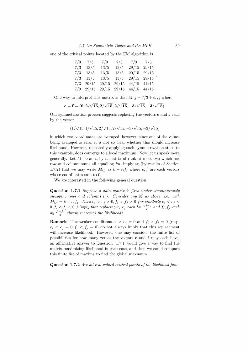
one of the critical points located by the EM algorithm is

7/3 7/3 7/3 7/3 7/3 7/37/3 13/5 13/5 13/5 29/15 29/157/3 13/5 13/5 13/5 29/15 29/157/3 13/5 13/5 13/5 29/15 29/157/3 29/15 29/15 29/15 44/15 44/157/3 29/15 29/15 29/15 44/15 44/15

.

One way to interpret this matrix is that Mi,j = 7/3 + eifj where

e = f = (0,2/√

15,2/√

15,2/√

15,−3/√

15,−3/√

15).

Our symmetrization process suggests replacing the vectors e and f eachby the vector

(1/√

15, 1/√

15, 2/√

15, 2/√

15,−3/√

15,−3/√

15)

in which two coordinates are averaged; however, since one of the valuesbeing averaged is zero, it is not so clear whether this should increaselikelihood. However, repeatedly applying such symmetrization steps tothis example, does converge to a local maximum. Now let us speak moregenerally. Let M be an n by n matrix of rank at most two which hasrow and column sums all equalling kn, implying (by results of Section1.7.2) that we may write Mi,j as k + eifj where e, f are each vectorswhose coordinates sum to 0.

We are interested in the following general question:

Question 1.7.1 Suppose a data matrix is fixed under simultaneouslyswapping rows and columns i, j. Consider any M as above, i.e. withMi,j = k + eifj. Does ei > ej > 0, fi > fj > 0 (or similarly ei < ej <

0, fi < fj < 0 ) imply that replacing ei, ej each by ei+ej

2 and fi, fj eachby fi+fj

2 always increases the likelihood?

Remarks The weaker conditions ei > ej = 0 and fi > fj = 0 (resp.ei < ej = 0, fi < fj = 0) do not always imply that this replacementwill increase likelihood. However, one may consider the finite list ofpossibilities for how many zeroes the vectors e and f may each have;an affirmative answer to Question 1.7.1 would give a way to find thematrix maximizing likelihood in each case, and then we could comparethis finite list of maxima to find the global maximum.

Question 1.7.2 Are all real-valued critical points of the likelihood func-

40 Contents

tion obtained by setting some number of coordinates in the e and f vec-tors to zero and then averaging by the above process so that the eventualvectors e and f have all positive coordinates equal to each other and allnegative coordinates equal to each other? This seems to be true in manyexamples.

One may check that the example discussed in Chapter 1 of Pachter andSturmfels (2005) gives another instance where this averaging approachleads quickly to what appears to be a global maximum. Namely, giventhe data matrix

4 2 2 22 4 2 22 2 4 22 2 2 4

and a particular starting point, the EM algorithm converges to the saddlepoint

148

4 2 3 32 4 3 33 3 3 33 3 3 3

,

whose entries may be written asMi,j = 1/48(3+aibj) for a = (−1,1,0,0)and b = (−1,1,0,0). Averaging −1 with 0 and 1 with the other 0 simul-taneously in a and b immediately yields the global maximum directlyby symmetrizing the saddle point, i.e. rather than finding it by runningthe EM algorithm repeatedly from various starting points.

An affirmative answer to Question 1.7.1 would imply several things.It would yield a (positive) solution to the 100 Swiss Franks problem, asdiscussed in Section 1.7.3. More generally, it would explain in a ratherprecise way how certain symmetries in data seem to impose symmetryon the global maxima of the maximum likelihood function. Moreover itwould suggest good ways to look for global maxima, as well as constrain-ing them enough that in some cases they can be characterized, as wedemonstrate for the 100 Swiss Franks problem. To make this concrete,one thing it would tell us for an n by n data matrix which is fixed bythe Sn action simultaneously permuting rows and columns in the sameway, is that any probability matrix maximizing likelihood for such a datamatrix will have at most two distinct types of rows.

We do not know the answer to this question, but we do prove that thistype of averaging will at least give a critical point within the subspace


in which ei, ej , fi, fj may vary freely but all other parameters are heldfixed. Data also provide evidence that the answer to the question mayvery well be yes. At the very least, this type of averaging appears to bea good heuristic for seeking local maxima, or at least finding a way tocontinue to increase maximum likelihood beyond what it is at a criticalpoint one reaches. Moreover, while real data are unlikely to have thesesymmetries, perhaps it could come close, and this could still be a goodheuristic to use in conjunction with the EM algorithm.

1.7.2 Preservation of Marginals and Some Consequences

Proposition 1.7.1 Given a two-way table in which all row and columnsums (i.e. marginals) are equal, then for M to maximize the likelihoodfunction among matrices of a fixed rank, the row and column sums ofM must be equal.

We prove the case mentioned in the abstract, which should generalizeby adjusting exponents and ratios in the proof. It may very well alsogeneralize to distinct marginals and tables with more rows and columns.

Proof Let R1, R2, R3, R4 be the row sums of M . Suppose R1 ≥ R2 ≥R3 > R4; other cases will be similar. Choose δ so that R3 = (1 +δ)R4. We will show that multiplying row 4 by any 1 + ε with 0 <

ε < min(1/4, δ/2) will strictly increase L, giving a contradiction to M

maximizing L. The result for column sums follows by symmetry.Let us write L(M ′) for the new matrix M ′ in terms of the variables

xi,j for the original matrix M , so as to show that L(M ′) > L(M). Thefirst inequality below is proven in Lemma 1.7.1.

L(M ′) =(1 + ε)10(

∏4i=1 xi,i)

4(∏i6=j xi,j)

2

R1 +R2 +R3 + (1 + ε)R4)40

>(1 + ε)10(

∏4i=1 xi,i)

4(∏i 6=j xi,j)

2

[(1 + 1/4(ε− ε2))(R1 +R2 +R3 +R4)]40

=(1 + ε)10(

∏4i=1 xi,i)

4(∏i 6=j xi,j)

2

[(1 + 1/4(ε− ε2))4]10[R1 +R2 +R3 +R4]40

=(1 + ε)10(

∏4i=1 xi,i)

4(∏i 6=j xi,j)

2

[1 + 4(1/4)(ε− ε2) + 6(1/4)2(ε− ε2)2 + · · ·+ (1/4)4(ε− ε2)4]10[∑4i=1Ri]40

42 Contents

≥ (1 + ε)10

(1 + ε)10· L(M)

Lemma 1.7.1 If ε < min(1/4, δ/2) and R1 ≥ R2 ≥ R3 = (1 + δ)R4,then R1 +R2 +R3 + (1 + ε)R4 < (1 + 1/4(ε− ε2))(R1 +R2 +R3 +R4).

Proof It is equivalent to show εR4 < (1/4)(ε)(1− ε)∑4i=1Ri. However,

(1/4)(ε)(1− ε)(4∑i=1

Ri) ≥ (3/4)(ε)(1− ε)(1 + δ)R4 + (1/4)(ε)(1− ε)R4

> (3/4)(ε)(1− ε)(1 + 2ε)R4 + (1/4)(ε)(1− ε)R4

= (3/4)(ε)(1 + ε− 2ε2)R4 + (1/4)(ε− ε2)R4

= εR4 + [(3/4)(ε2)− (6/4)(ε3)]R4 − (1/4)(ε2)R4

= εR4 + [(1/2)(ε2)− (3/2)(ε3)]R4

≥ εR4 + [(1/2)(ε2)− (3/2)(ε2)(1/4)]R4

> εR4.

Corollary 1.7.1 There exist vectors (e1, e2, e3, e4) and (f1, f2, f3, f4)such that

∑4i=1 ei =

∑4i=1 fi = 0 and Mi,j = K + eifj. Moreover, K

equals the average entry size.

In particular, this tells us that L may be maximized by treating it as afunction of just six variables, namely e1, e2, e3, f1, f2, f3, since e4, f4 arealso determined by these; changing K before solving this maximizationproblem simply has the impact of multiplying the entire matrix M thatmaximizes likelihood by a scalar.

Let E be the deviation matrix associated to M , where Ei,j = eifj .

Question 1.7.3 Another natural question to ask, in light of this corol-lary, is whether the matrix of rank at most r maximizing L is expressibleas the sum of a rank one matrix and a matrix of rank at most r− 1 thatmaximizes L among matrices of rank at most r − 1.

Remarks When we consider matrices with fixed row and column sums,


then we may ignore the denominator in the likelihood function and sim-ply maximize the numerator.

Corollary 1.7.2 If M which maximizes L has ei = ej, then it also hasfi = fj. Consequently, if it has ei 6= ej, then it also has fi 6= fj.

Proof One consequence of having equal row and column sums is that itallows the likelihood function to be split into a product of four functions,one for each row, or else one for each column; this is because the sum ofall table entries equals the sum of those in any row or column multipliedby four, allowing the denominator to be written just using variables fromany one row or column. Thus, once the vector e is chosen, we find thebest possible f for this given e by solving four separate maximizationproblems, one for each fi, i.e. one for each column. Setting ei = ejcauses the likelihood function for column i to coincide with the likelihoodfunction for column j, so both are maximized at the same value, implyingfi = fj .

Next we prove a slightly stronger general fact for matrices in whichrows and columns i, j may simultaneously be swapped without changingthe data matrix:

Proposition 1.7.2 If a matrix M maximizing likelihood has ei > ej > 0,then it also has fi > fj > 0.

Proof Without loss of generality, say i = 1, j = 3. We will show that ife1 > e3 and f1 < f3, then swapping columns one and three will increaselikelihood, yielding a contradiction. Let

L1(e1) = (1/4 + e1f1)4(1/4 + e1f2)2(1/4 + e1f3)2(1/4 + e1f4)2

and

L3(e3) = (1/4 + e2f1)2(1/4 + e2f2)2(1/4 + e3f3)4(1/4 + e3f4)2,

namely the contributions of rows 1 and 3 to the likelihood function. Let

K1(e1) = (1/4 + e1f3)4(1/4 + e1f2)2(1/4 + e1f1)2(1/4 + e1f4)2

and

K3(e3) = (1/4 + e3f3)2(1/4 + e3f2)2(1/4 + e3f1)4(1/4 + e3f4)2,

so that after swapping the first and third columns, the new contribution

44 Contents

to the likelihood function from rows one and three is K1(e1)K3(e3).Since the column swap does not impact that contributions from rows2 and 4, the point is to show K1(e1)K3(e3) > L1(e1)L3(e3). Ignoringcommon factors, this reduces to showing

(1/4 + e1f3)2(1/4 + e3f1)2 > (1/4 + e1f1)2(1/4 + e3f3)2,

in other words

(1/16+1/4(e1f3+e3f1)+e1e3f1f3)2 > (1/16+1/4(e1f1+e3f3)+e1e3f1f3)2,

namely e1f3 + e3f1 > e1f1 + e3f3. But since e3 < e1, f1 < f3, we have0 < (e1 − e3)(f3 − f1) = (e1f3 + e3f1) − (e1f1 + e3f3), just as needed.

Question 1.7.4 Does having a data matrix which is symmetric withrespect to transpose imply that matrices maximizing likelihood will alsobe symmetric with respect to transpose?

Perhaps this could also be verified again by averaging, similarly towhat we suggest for involutions swapping a pair of rows and columnssimultaneously.

1.7.3 The 100 Swiss Franks Problem

We use the results derived to far to show how to reduce the 100 SwissFranks problem to Question 1.7.1. Thus, an affirmative answer to Ques-tion 1.7.1 would provide a mathematical proof formally that the threetables in 1.2 a) are global maxima of the log-likelihood function for thebasic LC model with r = 2 and data given in (1.9).

Theorem 1.7.1 If the answer to Question 1.7.1 is yes, then the 100Swiss Franks problem is solved.

Proof Proposition 1.7.1 showed that for M to maximize L, M must haverow and column sums which are all equal to the quantity which we callR1, R2, R3, R4, C1, C2, C3, or C4 at our convenience. The denominatorof L may therefore be expressed as (4C1)10(4C2)10(4C3)10(4C4)10 or as(4R1)10(4R2)10(4R3)10(4R4)10, enabling us to rewrite L as a product offour smaller functions using distinct sets of variables.

Note that letting S4 simultaneously permute rows and columns willnot change L, so let us assume the first two rows of M are linearly


independent. Moreover, we may choose the first two rows in such a waythat the next two rows are each nonnegative combinations of the firsttwo. Since row and column sums are all equal, the third row, denoted v3,is expressible as xv1 + (1− x)v2 for v1, v2 the first and second rows andx ∈ [0, 1]. One may check that M does not have any row or column withvalues all equal to each other, because if it had one, then it would havethe other, reducing to a three by three problem which one may solve,and one may check that the answer does not have as high of likelihoodas

3 3 2 23 3 2 22 2 3 32 2 3 3

.

Proposition 1.7.3 will show that if the answer to Question 1.7.1 is yes,then for M to maximize L, we must have x = 0 or x = 1, implying row3 equals either row 1 or row 2, and likewise row 4 equals one of the firsttwo rows. Proposition 1.7.4 shows M does not have three rows all equalto each other, and therefore must have two pairs of equal rows. Thus,the first column takes the form (a, a, b, b)T , so it is simply a matter ofoptimizing a and b, then noting that the optimal choice will likewiseoptimize the other columns (by virtue of the way we broke L into aproduct of four expressions which are essentially the same, one for eachcolumn). Thus, M takes the form

a a b b

a a b b

b b a a

b b a a

since this matrix does indeed have rank two. Proposition 1.7.5 showsthat to maximize L one needs 2a = 3b, finishing the proof.

Proposition 1.7.3 If the answer to Question 1.7.1 is yes, then row 3equals either row 1 or row 2 in any matrix M which maximizes likelihood.Similarly, each row i with i > 2 equals either row 1 or row 2.

Proof M3,3 = xM1,3 + (1 − x)M2,3 for some x ∈ [0, 1], so M3,3 ≤max(M1,3,M2,3). If M1,3 = M2,3, then all entries of this column areequal, and one may use calculus to eliminate this possibility as fol-lows: either M has rank one, and then we may replace column three

46 Contents

by (c, c, 2c, c)T for suitable constant c to increase likelihood, since thisonly increases rank to at most two, or else the column space of M isspanned by (1, 1, 1, 1)T and some (a1, a2, a3, a4) with

∑ai = 0; specifi-

cally, column three equals (1/4, 1/4, 1/4, 1/4) +x(a1, a2, a3, a4) for somex, allowing its contribution to the likelihood function to be expressedas a function of x whose derivative at x = 0 is nonzero, provided thata3 6= 0, implying that adding or subtracting some small multiple of(a1, a2, a3, a4)T to the column will make the likelihood increase. Ifa3 = 0, then row three is also constant, i.e. e3 = f3 = 0. But then, anaffirmative answer to the second part of Question 1.7.1 will imply thatthis matrix does not maximize likelihood.

Suppose, on the other hand, M1,3 > M2,3. Our goal then is to showx = 1. By Proposition 1.7.1 applied to columns rather than rows, weknow that (1, 1, 1, 1) is in the span of the rows, so each row may bewritten as 1/4(1, 1, 1, 1) + cv for some fixed vector v whose coordinatessum to 0. Say row 1 equals 1/4(1, 1, 1, 1) + kv for k = 1. Writing rowthree as 1/4(1, 1, 1, 1) + lv, what remains is to rule out the possibilityl < k. However, Proposition 1.7.2 shows that l < k and a1 < a3

together imply that swapping columns one and three will yield a newmatrix of the same rank with larger likelihood.

Now we turn to the case of l < k and a1 ≥ a3. If a1 = a3 then swap-ping rows one and three will increase likelihood. Assume a1 > a3. ByCorollary 1.7.1, we have (e1, e2, e3, e4) with e1 > e3 and (f1, f2, f3, f4)with f1 > f3. Therefore, if the answer to Question 1.7.1 is yes, thenreplacing e1, e3 each by e1+e3

2 and f1, f3 each by f1+f32 yields a matrix

with larger likelihood, completing the proof.

Proposition 1.7.4 In any matrix M maximizing L among rank 2 ma-trices, no three rows of M are equal to each other.

Proof Without loss of generality, if M had three equal rows, then M

would take the forma c e g

b d f h

b d f h

b d f h

but then the fact that M maximizes L ensures d = f = h and c = e = g

since L is a product of four expressions, one for each column, so that thesecond, third and fourth columns will all maximize their contribution to

1.8 Conclusions 47

L in the same way. Since all row and column sums are equal, simplealgebra may be used to show that all entries must be equal. However,we have already shown that such matrices do not maximize L.

Proposition 1.7.5 To maximize M requires a, b related by 2a = 3b.

Proof We must maximize a6b4

(8a+8b)10 . We may assume a + b = 1 sincemultiplying the entire matrix by a constant does not change L, so wemaximize (1/8)10a6b4 with b = 1 − a; in other words, we maximizef(a) = a6(1 − a)4. But solving f ′(a) = 0 = 6a5(1 − a)4 + a6(4)(1 −a)3(−1) = a5(1−a)3[6(1−a)− 4a] yields 6(1−a)− 4a = 0, so a = 6/10and b = 4/10 as desired.

1.8 Conclusions

In this paper we have reconsidered the classical latent class model forcontingency table data and studied its geometric and statistical prop-erties. We have exploited theoretical and computational tools from al-gebraic geometry to display the complexities of the latent class model.We have focused on the problem of maximum likelihood estimation andhave studied the singularities arising from symmetries in the contingencytable data and the multiple maxima that appear to result from these.We have given an informal characterization of this problem, but a strictmathematical proof of the existence of identical multiple maxima haseluded us; we describe elements of a proof in a separate section.

We have also applied LC models to synthetic data and to data arisingfrom two real-life applications. In one, the model is quite simple andmaximum likelihood estimation poses little problems, whereas in theother high-dimensional example various issues, computational as well asmodel-based, arise. From the computational standpoint, both the EMand the Newton-Raphson algorithm are especially vulnerable to prob-lems of multimodality and provide little in the way of clues regardingthe dimensionality difficulties associated with the underlying structure ofLC models. Furthermore, the seemingly singular behavior of the Fisherinformation matrix at the MLE that we observe even for well-behaved,identifiable models is an additional element of complexity.

Based on our work, we would advise practitioners to exercise cautionin applying LC models, especially to sparse data. They have a tremen-dous heuristic appeal and in some examples provide a clear and convinc-

48 Contents

ing description of the data. But in many situations, the kind of complexbehavior explored in this paper may lead to erroneous inferences.

1.9 Acknowledgments

This research was supported in part by the National Institutes of Healthunder Grant No. R01 AG023141-01, by NSF Grant DMS-0631589, andby a grant from the Pennsylvania Department of Health through theCommonwealth Universal Research Enhancement Program, all to theDepartment of Statistics to Carnegie Mellon University, and by NSFGrant DMS-0439734 to the Institute for Mathematics and Its Appli-cation at the University of Minnesota. We thank Bernd Sturmfels forintroducing us to the 100 Swiss Franks problem, which motivated muchof this work, and for his valuable comments and feedback.

References

Allman, E.S. and Rhodes, J.A. (2006). Phylogenetic invariants for stationarybase composition, Journal of Symbolic Computation, 41, 138–150.

Allman, E. and Rhodes, J.A. (2007). Phylogenetic ideals and varieties for thegeneral Markov model, Advances in Applied Mathematics, to appear.

Anderson, D.R., Burham, K.P., and White, G.C. (1994). AIC model selectionin overdispersed capture-recature data. Ecology, 75, 1780–1793.

Anderson, T.W. (1954). On estimation of parameters in latent structure anal-ysis, Psychometrika, 19, 1–10.

Bandeen-Roche, K., Miglioretti, D.L., Zeger, S., and Rathouz, P.J. (1997).Latent variable regressionfor multiple discrete outcomes, Journal of theAmerican Statistical Association, 92, 1375–1386.

Benedetti, R. (1990). Real algebraic and semi-algebraic sets, Hermann.Catalisano, M.V., Geremita, A.V. and Gimigliano, A. (2002). Ranks of tensors,

secant varieties of Segre varieties and fat points, Linear Algebra and ItsApplications, 355, 263–285.

Catalisano, M.V., Geremita, A.V. and Gimigliano, A. (2003). Erratum to:“Ranks of tensors, secant varieties of Segre varieties and fat points,” Lin-ear Algebra and Its Applications, 367, 347–348.

Clogg, C. and Goodman, L. (1984). Latent Structure Analysis of a Set ofMultidimensional Contingency Tables, Journal of the American Statisti-cal Association, 79, 762–771.

Cohen, J.E. and Rothblum, U.G. (1993). Nonnegative rank, decompositionsand factorisations of nonnegative matrices. Linear Algebra and Its Appli-cations, 190, 149–168.

Cox, D.A., Little, J. and O’Shea, D. (1996). Ideals, Varieties, and Algorithms:An Introduction to Computational Algebraic Geometry and CommutativeAlgebra, Springer-Verlag.

Cowell, R.G., Dawid, P.A., Lauritzen, S.L. and Spiegelhalter, D.J. (1999).Probabilistic Networks and Expert Systems, Springer-Verlag.

Erosheva, E.A. (2002). Grade of Membership and Latent Structure Modelswith Application to Disability Survey Data. PhD thesis, Department ofStatistics, Carnegie Mellon University.

Erosheva, E.A. (2005). Comparing latent structures of the grade of member-ship, Rasch and latent class models, Psychometrika, 70, 619–626.

Erosheva, E.A., Fienberg, S.E., and Joutard, C. (2007). Describing disabil-ity through individual-level mixture models for multivariate binary data,

49

50 References

Annals of Applied Statistics, 1, in press.Espeland, M. A. (1986). A general class of models for discrete multivariate

data, Communications in Statistics: Simulation and Computation, 15,405–424.

Garcia, L.D. (2004). Algebraic Statistics in Model Selection, Proceedings of the20th Annual Conference on Uncertainty in Artificial Intelligence (UAI-04), 177–18, AUAI Press.

Garcia, L., Stillman, M. and Sturmfels, B. (2005). Algebraic Geometry ofBayesian Networks, Journal of Symbolic Computation, 39, 331–355.

Geiger, D., Heckerman, D., King, H. and Meek, C. (2001). Stratified Exponen-tial Families: Graphical Models and Model Selection, Annals of Statistics,29(2), 505–529.

Gibson, W.A. (1955). An extension of Anderson’s solution for the latent struc-ture equations, Psychometrika, 20, 69–73.

Goodman, L. (1979). On the estimation of parameters in latent structureanalysis, Psychometrika, 44(1), 123–128.

Goodman, L. (1974). Exploratory latent structure analysis using both identi-fiable and unidentifiable models, Biometrika, 61, 215–231.

Greuel, G.-M. , Pfister, G. and H. Schonemann. (2005). Singular 3.0. A Com-puter Algebra System for Polynomial Computations. Centre for Com-puter Algebra, University of Kaiserslautern.http://www.singular.uni-kl.de.

Haber, M. (1986). Testing for pairwise independence, Biometrics, 42, 429–435.Haberman, S.J. (1974). Log-linear models for frequency tables derived by in-

direct obsertations: maximum likelihood equations, Annals of Statistics,2, 911–924.

Haberman, S.J. (1988). A stabilized Newton-Raphson algorithm for log-linearmodels for frequency tables derived by indirect observation, SociologicalMethodology, 18, 193–211.

Harris, J. (1992). lgebraic Geometry: A First Course, Springer-Verlag.Henry, N.W.. and Lazarfeld, P.F. (1968). Latent Structure Analysis, Houghton

Mufflin Company.Kocka, T. and Zhang, N. L. (2002). Dimension correction for hierarchical

latent class models, PProceeding of the Eighteenth Conference on Uncer-tainty in Artificial Intelligence (UAI-02), 267–274, Morgan Kaufmann.

Kruskal, J.B. (1975). More factors than subjects, tests and treatments: Anindeterminacy theorem for canonical decomposition and individual differ-ences scaling, Psychometrica, 41, 281–293.

Landsberg, J.M. and Manivel, L. (2004). On the ideals of secant varieties ofSegre varieties, Foundations of Computational Mathematics, 4, 397–422.

Lauritzen, S.L. (1996). Graphical Models, Oxford University Press.Madansky, A. (1960). Determinantial methods in latent class analysis, Psy-

chometrica, 25, 183–198.Mond, D.M.Q., Smith, J.Q. and Van Straten, D. (2003) Stochastic factorisa-

tions, sandwiched simplices and the topology of the space of explanations,Proceeding of the Royal Society of London, Series A, 459, 2821–2845.

Monto, A.S., Koopman, J.S., and Longini, I.M. (1985). Tecumseh study ofillness. XIII. Influenza infection and disease. American Journal of Epi-demiology, 121, 811–822.

Pachter, L. and Sturmfels, B., eds. (2005). Algebraic Statistics for Computa-tional Biology, Cambridge University Press.

References 51

Redner, R.A. and Walker, H.F. (1984). Mixture densities, maximum likelihoodand the EM algorithm, SIAM Review, 26, 195–239.

Rusakov, D. and Geigerm, D. (2005). Asymptotic model selection for naiveBayesian networks, Journal of Machine Learning Research, 6, 1–35.

Settimi, R. and Smith, J.Q. (2005). Geometry, moments and conditional inde-pendence trees with hidden variables, Annals of Statistics, 28, 1179-1205.

Settimi, R. and Smith, J.Q. (1998). On the geometry of Bayesian graphicalmodels with hidden variables, Proceedings of the Fourteenth Conferenceon Uncertainty in Artificial Intel ligence, 479–472, Morgan KaufmannPublishers.

Smith, J.Q. and Croft, J. (2003). Bayesian networks for discrete multivariatedata: an algebraic approach to inference, Journal of Multivariate Analy-sis, 84, 387–402.

Strassen, V. (1983). Rank and optimal computation of generic tensors, LinearAlgebra and Its Applications, 52/53, 654–685.

Humphreys, K. and Titterington, D.M. (2003). Variational approximationsfor categorical causal modeling with latent variables. Psychometrika, 68,391–412.

Uebersax, J. (2006a). LCA Frequently Asked Questions (FAQ).http://ourworld.compuserve.com/homepages/jsuebersax/faq.htm

Uebersax, J. (2006b). Latent Class Analysis, A web-site with bibliography,software, links and FAQ for latent class analysis.http://ourworld.compuserve.com/homepages/jsuebersax/index.htm

Watanabe, S. (2001). Algebraic analysis for nonidentifiable learning machines,Neural Computation, 13, 899933.

Zhou, Y. (2007). Maximum Likelihood Estimation in Latent Class Models.Manuscript.

Maximum Likelihood Estimation in Latent Class Models …arinaldo/papers/Fienberg_Hersh_Rinaldo_Zhou_20… · Maximum Likelihood Estimation in Latent Class Models For Contingency Table

Documents