Maximum Data Gathering in Networked Sensor Systems

Maximum Data Gathering in Networked Sensor Systems�

Bo Hong and Viktor K. Prasanna

University of Southern California, Los Angeles CA 90089-2562

�bohong, prasanna � @usc.edu

Abstract

We focus on data gathering problems in energy-constrained networked sensor systems. We study store-

and-gather problems where data are locally stored at the sensors before the data gathering starts, and

continuous sensing and gathering problems that model time critical applications. We show that these

problems reduce to maximization of network flow under vertex capacity constraint. This flow problem

in turn reduces to a standard network flow problem. We develop a distributed and adaptive algorithm to

optimize data gathering. This algorithm leads to a simple protocol that coordinates the sensor nodes in

the system. Our approach provides a unified framework to study a variety of data gathering problems in

networked sensor systems. The performance of the proposed method is illustrated through simulations.

�Supported by the National Science Foundation under award No. IIS-0330445 and in part by DARPA under contract

F33615-02-2-4005.

1

1 Introduction

State-of-the-art sensors (e.g. Smart Dust [20]) are powered by batteries. Replenishing energy by

replacing the batteries is infeasible since the sensors are typically deployed in harsh terrains. Also, the

cost of replacing batteries can be prohibitively high. These sensors, which are usually unattended, need

to operate over a long period of time after deployment. Energy efficiency is thus critical. Techniques

ranging from low power hardware design [2, 15] and energy aware routing [8, 19] to application level

optimizations [18, 21] have been proposed to improve energy efficiency of networked sensor systems.

An important application of networked sensor systems is to monitor the environment. Examples of

such applications include vehicle tracking and classification in the battle field, patient health monitoring,

pollution detection, etc. In these applications, a fundamental operation is to sense the environment and

transmit the sensed data to the base station for further processing. In this paper, we study energy efficient

data gathering in networked sensor systems from an algorithmic perspective.

Compared with sensing and computation, communication is the most expensive operation (in terms

of energy consumption) in the context of data gathering [1]. Generally, data transfers are performed

via multi-hop communications where each hop is a short-range communication. This is due to the well

known fact that long-distance wireless communication is expensive in terms of both implementation

complexity and energy dissipation, especially when using the low-lying antennae and near-ground chan-

nels typically found in networked sensor systems. Short-range communication also enables efficient

spatial frequency re-use. A challenging problem with multi-hop communications is the efficient transfer

of data through the system when the sensors have energy constraints.

Some variations of the problem have been studied recently. In [11], data gathering is assumed to be

performed in rounds and each sensor can communicate (in a single hop) with the base station and all

2

other sensors. The total number of rounds is then maximized under a given energy constraint on the sen-

sors. In [14], a non-linear programing formulation is proposed to explore the trade-offs between energy

consumed and the transmission rate. It models the radio transmission energy according to Shannon’s

theorem. In [16], the data gathering problem is formulated as a linear programing problem and a ��

approximation algorithm is proposed. This algorithm further leads to a distributed heuristic.

Our study departs from the above with respect to the problem definition as well as the solution tech-

nique. For short-range communications, the difference in the energy consumption between sending and

receiving a data packet is almost negligible. We adopt the reasonable approximation that sending a data

packet consumes the same amount of energy as receiving a data packet [1]. The study in [14] and [16]

differentiate the energy dissipated for sending and receiving data. Although the resulting problem for-

mulations are indeed more accurate than ours, the improvement in accuracy is marginal for short-range

communications.

In [11], each sensor generates exactly one data packet per round (a round corresponds to the occur-

rence of an event in the environment) to be transmitted to the base station. The system is assumed to

be fully connected. The study in [11] also considers a very simple model of data aggregation where

any sensor can aggregate all the received data packets into a single output data packet. In our system

model, each sensor communicates with a limited number of neighbors due to the short range of the com-

munications, resulting in a general graph topology for the system. We study store-and-gather problems

where data are locally stored on the sensors before the data gathering starts, and continuous sensing and

gathering problems that models time critical applications. A unified flow optimization formulation is

developed for the two classes of problems.

Our focus in this paper is to maximize the throughput or volume of data received by the base station.

3

Such an optimization objective is abstracted from a wide range of applications in which the base station

needs to gather as much information as possible. Some applications proposed for the networked sensor

systems may have different optimization objectives. For example, the balanced data transfer problem [6]

is formulated as a linear programming problem where a ‘minimum achieved sense rate’ is set for every

individual node. In [5], data gathering is considered in the context of energy balance. A distributed

protocol is designed to ensure that the average energy dissipation per node is the same throughout the

execution of the protocol. However, these issues are not the focus of this paper.

By modeling the energy consumption associated with each send and receive operation, we formulate

the data gathering problem as a constrained network flow optimization problem where each each node �

is associated with a capacity constraint �� , so that the total amount of flow going through � (incoming

plus outgoing flow) does not exceed �� . We show that such a formulation models a variety of data

gathering problems (with energy constraint on the sensor nodes).

The constrained flow problem reduces to the standard network flow problem, which is a classical flow

optimization problem. Many efficient algorithms have been developed ([3]) for the standard network

flow problem. However, in terms of decentralization and adaptation, these well known algorithms are

not suitable for data gathering in networked sensor systems. In this paper, we develop a decentralized

and adaptive algorithm for the maximum network flow problem. This algorithm is a modified version

of the Push-Relabel algorithm [7]. In contrast to the Push-Relabel algorithm, it is adaptive to changes in

the system. It finds the maximum flow in��

time, where�

is the number of adaptation

operations, ��

is the number of nodes, and ��

is the number of links.

The above algorithm can be used to solve both store-and-gather problems and continuous sensing and

gathering problems. For the continuous sensing and gathering problems, we develop a simple distributed

4

protocol based on the algorithm. The performance of this protocol is studied through simulations. Be-

cause the store-and-gather problems are by nature off-line problems, we do not develop a distributed

protocol for this class of problems.

The rest of the paper is organized as follows. The data gathering problems are discussed in Section 2.

We show that these problems reduce to network flow problem with constraint on the vertices. In Sec-

tion 3, we develop a mathematical formulation of the constrained network flow problem and show that

it reduces to a standard network flow problem. In Section 4, we derive a relaxed form for the network

flow problem. A distributed and adaptive algorithm is then developed for this relaxed problem. A sim-

ple protocol based on this algorithm is presented in Section 4.3. Experimental results are presented in

Section 5. Section 6 concludes this paper.

2 Data Gathering with Energy Constraint

2.1 System Model

Suppose a network of sensors is deployed over a region. The location of the sensors are fixed and

known a priori. The system is represented by a graph � � �� , where�

is the set of sensor nodes.

� � �� if � � �

,��

and � is within the communication range of�. The set of successors

of � is denoted as � �� . Similarly, the set of predecessors of � is denoted as

� �� . The event is sensed by a subset of sensors��

. � is the base station to

which the sensed data are transmitted. Sensors�� in the network does not sense the event but

can relay the data sensed by��

.

Among the three categories (sensing, communication, and data processing) of power consumption,

a sensor node typically spends most of its energy in data communication. This includes both data

5

transmission and reception. Our energy model for the sensors is based on the first order radio model

described in [9]. The energy consumed by sensor � to transmit a � � bit data packet to sensor�

is

� �� , where �� is the energy required for transceiver circuitry to process

one bit of data, �� is the energy required per bit of data for transmitter amplifier, and� �� is the distance

between � and�. Transmitter amplifier is not needed by � to receive data and the energy consumed by �

to receive a � � bit data packet is � � �� . Typically, �� "!�#%$�& and ��'�(� )�+* � �,�-!�#%$�&.!�/� .

This effectively translates to �� 10 �� , especially when short transmission ranges ( 2 � / ) are

considered. For the discussion in the rest of this paper, we adopt the approximation that� �� 3� � for

� � �� . We further assume that no data aggregation is performed during the transmission of the data.

Communication link� � � � � has transmission bandwidth 4 �� . We do not require the communication

links to be identical. Two communication links may have different transmission latencies and/or band-

width. Symmetry is not required either. It may be the case that 4 ��65�4 �� . If� � �� 7!� � , then we define

4 �� )� .

An energy budget 8 � is imposed on each sensor node � . We assume that there is no energy constraint

on base station � . To simplify our discussions, we ignore the energy consumption of the sensors when

sensing the environment. However, the rate at which sensor � � � � can collect data from the environment

is limited by the maximum sensing capability 9 � . We consider both store-and-gather problems and

continuous sensing and gathering problems. For the store-and-gather problems, 8 � represents the total

number of data packets that � can send and receive. For the continuous sensing and gathering problems,

8 � represents the total number of data packets that � can send and receive in one unit of time.

6

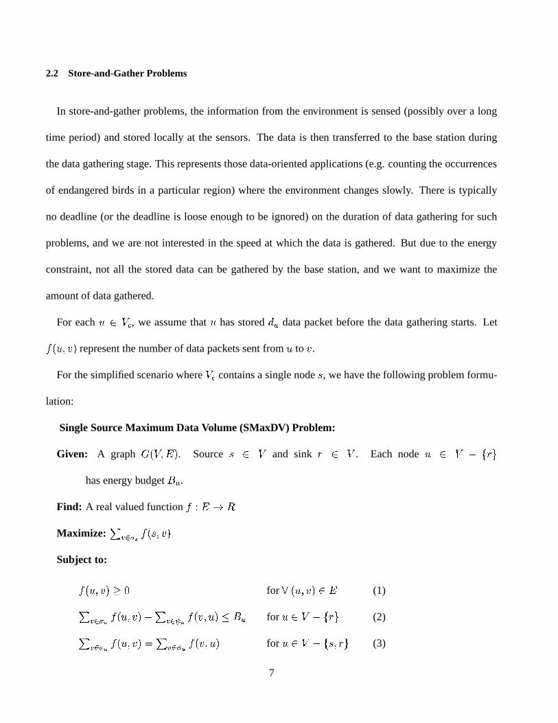
2.2 Store-and-Gather Problems

In store-and-gather problems, the information from the environment is sensed (possibly over a long

time period) and stored locally at the sensors. The data is then transferred to the base station during

the data gathering stage. This represents those data-oriented applications (e.g. counting the occurrences

of endangered birds in a particular region) where the environment changes slowly. There is typically

no deadline (or the deadline is loose enough to be ignored) on the duration of data gathering for such

problems, and we are not interested in the speed at which the data is gathered. But due to the energy

constraint, not all the stored data can be gathered by the base station, and we want to maximize the

amount of data gathered.

For each � � � �, we assume that � has stored

� � data packet before the data gathering starts. Let

� � � �� represent the number of data packets sent from � to�.

For the simplified scenario where��

contains a single node � , we have the following problem formu-

lation:

Single Source Maximum Data Volume (SMaxDV) Problem:

Given: A graph � � � � � � . Source � � �and sink � � �

. Each node � � � � ��

has energy budget 8 � .

Find: A real valued function��

Maximize: � ��

Subject to:

� � � �� for � � � � � � � � (1)

� �� 8 � for � � � � �� (2)

� �� for � � � � �� (3)

7

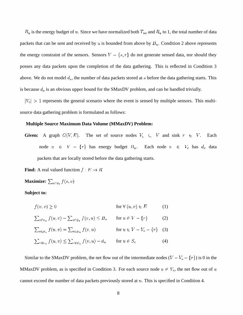
8 � is the energy budget of � . Since we have normalized both� �� and � � to 1, the total number of data

packets that can be sent and received by � is bounded from above by 8 � . Condition 2 above represents

the energy constraint of the sensors. Sensors� � �� do not generate sensed data, nor should they

posses any data packets upon the completion of the data gathering. This is reflected in Condition 3

above. We do not model��

, the number of data packets stored at � before the data gathering starts. This

is because��

is an obvious upper bound for the SMaxDV problem, and can be handled trivially.

�� represents the general scenario where the event is sensed by multiple sensors. This multi-

source data gathering problem is formulated as follows:

Multiple Source Maximum Data Volume (MMaxDV) Problem:

Given: A graph � � � � � � . The set of source nodes��

and sink � � �. Each

node � � � � �� has energy budget 8 � . Each node� � ��

has� � data

packets that are locally stored before the data gathering starts.



Subject to:

� � � �� for � � � � � � � � (1)

� �� 8 � for � � � � �� (2)

� �� for � � � � �� (3)

� �� for � �� (4)

Similar to the SMaxDV problem, the net flow out of the intermediate nodes (� � � �� ) is 0 in the

MMaxDV problem, as is specified in Condition 3. For each source node � � � �, the net flow out of �

cannot exceed the number of data packets previously stored at � . This is specified in Condition 4.

8

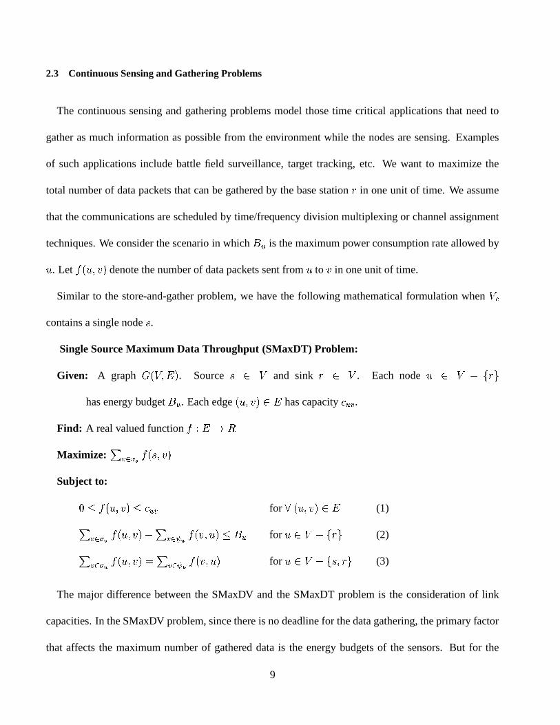
2.3 Continuous Sensing and Gathering Problems

The continuous sensing and gathering problems model those time critical applications that need to

gather as much information as possible from the environment while the nodes are sensing. Examples

of such applications include battle field surveillance, target tracking, etc. We want to maximize the

total number of data packets that can be gathered by the base station � in one unit of time. We assume

that the communications are scheduled by time/frequency division multiplexing or channel assignment

techniques. We consider the scenario in which 8 � is the maximum power consumption rate allowed by

� . Let� � � �� denote the number of data packets sent from � to

�in one unit of time.

Similar to the store-and-gather problem, we have the following mathematical formulation when� �

contains a single node � .Single Source Maximum Data Throughput (SMaxDT) Problem:

Given: A graph � � � � � � . Source � � �and sink � � �

. Each node � � � � ��

has energy budget 8 � . Each edge� � �� has capacity 4 � � .



Subject to:

� � � � � �� 4 �� for � � � �� (1)

� �� 8 � for � � � � �� (2)

� �� for � � � � �� (3)

The major difference between the SMaxDV and the SMaxDT problem is the consideration of link

capacities. In the SMaxDV problem, since there is no deadline for the data gathering, the primary factor

that affects the maximum number of gathered data is the energy budgets of the sensors. But for the

9

SMaxDT problem, the number of data packets that can be transferred over a link in one unit of time is

not only affected by the energy budget, but also bounded from above by the capacity of that link, as is

specified in Condition 1 above. For the SMaxDT problem, we do not model the impact of 9 � because 9 �

is an obvious upper bound of the throughput and can be handled trivially.

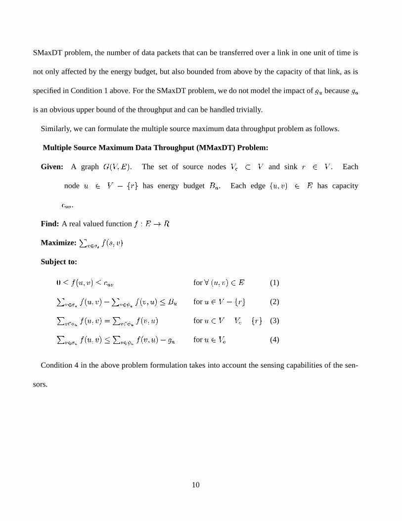
Similarly, we can formulate the multiple source maximum data throughput problem as follows.

Multiple Source Maximum Data Throughput (MMaxDT) Problem:

Given: A graph � � � � � � . The set of source nodes��

and sink � � �. Each

node � � � � �� has energy budget 8 � . Each edge� � ��

has capacity

4 �� .



Subject to:

� � � � � �� 4 �� for � � � �� (1)

� �� 8 � for � � � � �� (2)

� �� for � � � � � � � �� (3)

� �� 9 � for � � � � (4)

Condition 4 in the above problem formulation takes into account the sensing capabilities of the sen-

sors.

10

3 Flow Maximization with Constraint on Vertices

3.1 Problem Reductions

In this section, we present the formulation of the constrained flow maximization problem where the

vertices have limited capacities (CFM problem). The CFM problem is an abstraction of the four prob-

lems discussed in Section 2.

In the CFM problem, we are given a directed graph � � � � � � with vertex set�

and edge set�

. Vertex

� has capacity constraint � � � � . Edge� � �� starts from vertex � , ends at vertex

�, and has capacity

constraint 4 � � � � . If� � �� !� �

, we define 4 �� 3� . We distinguish two vertices in � , source � , and

sink � . A flow in � is a real valued function� � � � � that satisfies the following constraints:

1. � � � � � �� 4 � � for � � � � � � � � . This is the capacity constraint on edge� � �� .

2. � �� for � � � � � �� . This represents the flow conservation. The

net amount of flow that goes through any of the vertices, except � and&, is zero.

3. � �� for � � � � . This is the capacity constraint of vertex � . The

total amount of flow going through � cannot exceed � � . This condition differentiates the CFM

problem from the standard network flow problem.

The value of a flow�

, denoted as �

, is defined as � � �� , which is the net flow that

leaves � . In the CFM problem, we are given a graph with vertex and edge constraint, a source � , and a

sink � , and we wish to find a flow with the maximum value.

It is straight forward to show that the SMaxDV and the SMaxDT problems reduce to the CFM prob-

lem. By adding a hypothetical super source node, the MMaxDV and the MMaxDT problems can also

be reduced to SMaxDV and SMaxDT, respectively.

11

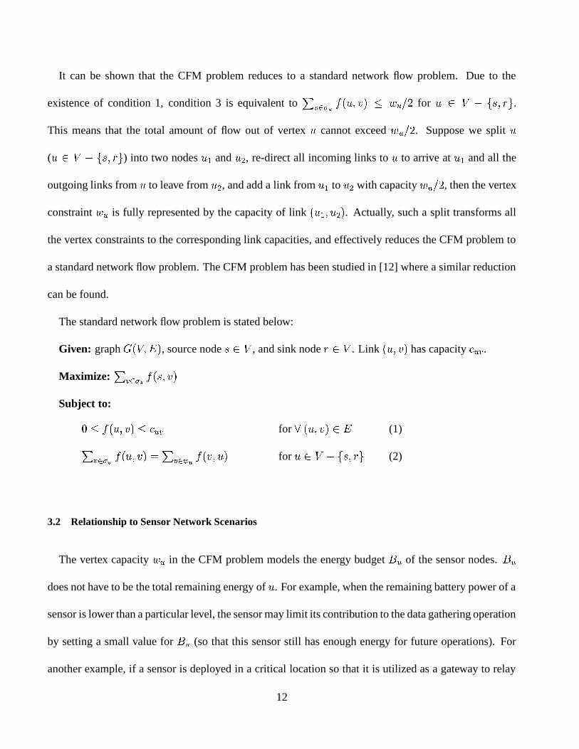
It can be shown that the CFM problem reduces to a standard network flow problem. Due to the

existence of condition 1, condition 3 is equivalent to � �� !�� for � � � � �� .This means that the total amount of flow out of vertex � cannot exceed � � !�� . Suppose we split �

( � � � � �� ) into two nodes �� and � , re-direct all incoming links to � to arrive at �� and all the

outgoing links from � to leave from � , and add a link from �� to � with capacity � � !�� , then the vertex

constraint � � is fully represented by the capacity of link� �� . Actually, such a split transforms all

the vertex constraints to the corresponding link capacities, and effectively reduces the CFM problem to

a standard network flow problem. The CFM problem has been studied in [12] where a similar reduction

can be found.

The standard network flow problem is stated below:

Given: graph � � � � � � , source node � � � , and sink node � � � . Link� � �� has capacity 4 �� .


Subject to:

� � � � � �� 4 �� for � � � �� (1)

� �� for � � � � �� (2)

3.2 Relationship to Sensor Network Scenarios

The vertex capacity � � in the CFM problem models the energy budget 8 � of the sensor nodes. 8 �

does not have to be the total remaining energy of � . For example, when the remaining battery power of a

sensor is lower than a particular level, the sensor may limit its contribution to the data gathering operation

by setting a small value for 8 � (so that this sensor still has enough energy for future operations). For

another example, if a sensor is deployed in a critical location so that it is utilized as a gateway to relay

12

data packets to a group of sensors, then it may limit its energy budget for a particular data gathering

operation, thereby conserving energy for future operations. These considerations can be captured by

vertex capacity � � in the CFM problem.

The edge capacity in the CFM problem models the communication rate (meaningful for continuous

sensing and gathering problems) between adjacent sensor nodes. The edge capacity captures the avail-

able communication bandwidth between two nodes, which may be less than the the maximum available

rate. For example, a node may reduce its radio transmission power to save energy, resulting in a less

than maximum communication rate. This capacity can also vary over time based on environmental

conditions. Our decentralized protocol results in an on-line algorithm for this scenario.

Because energy efficiency is a key consideration, various techniques have been proposed to explore

the trade-offs between processing/communication speed and energy consumption. This results in the

continuous variation of the performance of the nodes. For example, the processing capabilities may

change as a result of dynamic voltage scaling [13]. The data communication rate may change as a result

of modulation scaling [17]. As proposed by various studies on energy efficiency, it is necessary for

sensors to maintain a power management scheme, which continuously monitors and adjusts the energy

consumption and hence changes the computation and communication performance of the sensors. In

data gathering problems, these energy related adjustments translate to changes of parameters (node/link

capacities) in the problem formulations. Determining the exact reasons and mechanisms behind such

changes is beyond the scope of this paper. Instead, we focus on the development of data gathering

algorithms that can adapt to such changes.

13

Figure 1. An example of the relaxed network flow problem where 4 � � � � and 4 �� .

4 Distributed and Adaptive Algorithm To Maximize Flow

In this section, we first show that the maximum flow remains the same even if we relax the flow

conservation constraint. Then we develop a distributed and adaptive algorithm for the relaxed problem.

4.1 Relaxed Flow Maximization Problem

Consider the simple example in Figure 1 where � is the source, � is the sink, and � are the intermediate

nodes. Obviously, the flow is maximized when� � � � � � � � � � � � � � . Suppose � , � , and � form an

actual system and � has sent 10 data packets to � . Then � can send no more than 10 data packets to �even if � is allowed to transfer more to � . This means the actual system still works as if

� � � � � � � �even if we set

� � � � � �� .This leads to the following relaxed network flow problem:

Given: graph � � � � � � , source node � � � , and sink node � � � . Link� � �� has capacity 4 �� .


Subject to:

� � � � � �� 4 �� for � � � �� (1)

� �� for � � � � �� (2)

Condition 2 differentiates the relaxed and the standard network flow problem. In the relaxed problem,

the total flow out of a node can be equal to or larger than the total flow into the node. A feasible function

�(which satisfies the two constraints above) to the relaxed flow problem is called a relaxed flow in graph

14

� . �

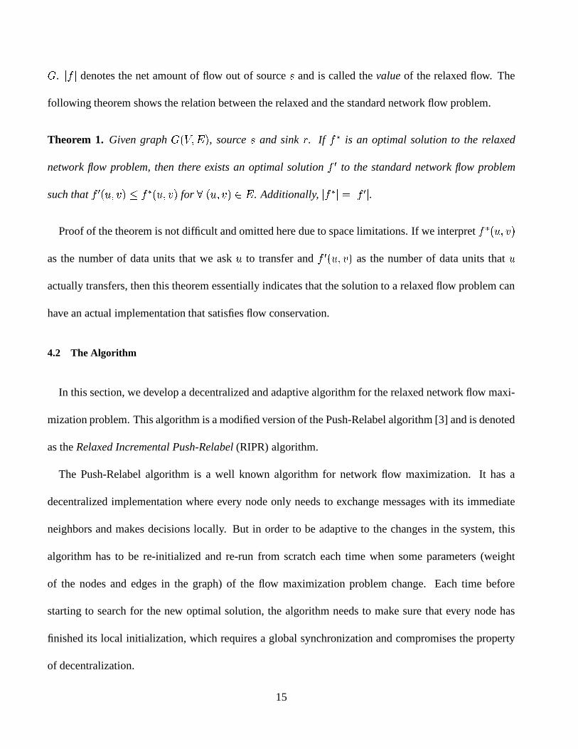
denotes the net amount of flow out of source � and is called the value of the relaxed flow. The

following theorem shows the relation between the relaxed and the standard network flow problem.

Theorem 1. Given graph � � � � � � , source � and sink � . If��

is an optimal solution to the relaxed

network flow problem, then there exists an optimal solution��

to the standard network flow problem

such that�� for � � � � � � � � . Additionally,

�� .

Proof of the theorem is not difficult and omitted here due to space limitations. If we interpret��

as the number of data units that we ask � to transfer and�� as the number of data units that �

actually transfers, then this theorem essentially indicates that the solution to a relaxed flow problem can

have an actual implementation that satisfies flow conservation.

4.2 The Algorithm

In this section, we develop a decentralized and adaptive algorithm for the relaxed network flow maxi-

mization problem. This algorithm is a modified version of the Push-Relabel algorithm [3] and is denoted

as the Relaxed Incremental Push-Relabel (RIPR) algorithm.

The Push-Relabel algorithm is a well known algorithm for network flow maximization. It has a

decentralized implementation where every node only needs to exchange messages with its immediate

neighbors and makes decisions locally. But in order to be adaptive to the changes in the system, this

algorithm has to be re-initialized and re-run from scratch each time when some parameters (weight

of the nodes and edges in the graph) of the flow maximization problem change. Each time before

starting to search for the new optimal solution, the algorithm needs to make sure that every node has

finished its local initialization, which requires a global synchronization and compromises the property

of decentralization.

15

In contrast to the Push-Relabel algorithm, our algorithm introduces the adaptation operation, which

is performed upon the current values of� � � � � � and

� � � � for � � �� . In other words, our algorithm

performs incremental optimization as the parameters of the system change. Our algorithm does not need

global synchronizations. Another difference is that our algorithm applies to the relaxed network flow

problem, rather than the standard one.

For the discussion below, let us first briefly re-state some notations for the network flow maximization

problem. For notational convenience, if edge� � �� 7!� � , we define 4 � � )� ; if the actual data transfer is

from � to�, we define

� �� . With these two definitions, if neither� � �� nor

�� belongs

to�

, then 4 �� 4�� , which implies that� � � �� . Of course,

� � � � � � � � � � � � �

implies that� � � � � � � , which essentially says that a node cannot send flow to itself. In this way,

we can define� � � �� over

� � �, rather than being restricted to

�.� � � � � � � � �� also allows

us to compute the total amount of flow into � as � �� , which equals � �� since

� �� if� � � � �6!� �

and� �� 6!� �

. With the definition of� � � �� thus extended, it is

easy to show that the relaxed network flow problem is equivalent to the following formulation:

Given: graph � � �� , source node � � �, and sink node � � �

. Link� � �� has capacity 4 �� .

4 �� )� if� � �� !� � .


Subject to:

� � � �� for � �� (1)

� � � �� 4 � � for � �� (2)

� �� for � � � � �� (3)

Given a direct graph � � � � � � , function�

is called a flow if it satisfies the three conditions in the

16

above problem; function�

is called a pre-flow if it satisfies conditions 1 and 2. Given � � � � � � and�

,

the residual capacity 4�� is given by 4 �� , and the residual network of � induced by�

is

�� , where�� 4�� . For each node � � �

, �� is defined as

�� , which is the total amount of flow into � .

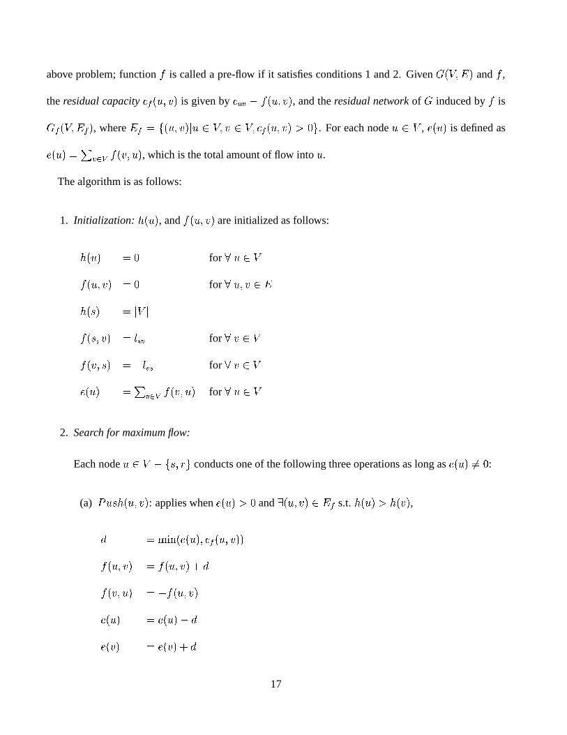
The algorithm is as follows:

1. Initialization:� � � � , and

� � � �� are initialized as follows:

� � � � )� for � � � �� )� for � � ��

� � � �� for � � � �� for � � � �

� � � � � �� for � � � �

2. Search for maximum flow:

Each node � � � � �� conducts one of the following three operations as long as � � � � 5�� :

(a) � � � � � � �� : applies when �� and �

� � �� s.t.� � � � � � � � �

,

� �� 4��

� � � � ��

� ��

17

(b) � � � � # � � � � � : applies when �� and

� � � � � � �� for � � � �� ,

� � � � � ��

3. Adaptation to changes in the system: For the flow maximization problem, the only possible change

that can occur in the system is the increase or decrease of the capacity of some edges. Suppose

the value of � �� changes to �� , the following four scenarios are considered when performing the

Adaptation� � �� operation:

(a) if �� and

� � � �� , do nothing.

(b) if �� and

� � � �� , then

� � � � � � � � � ��

� � � �� for � �� for � ��

� �� for � ��

(c) if �� and

� � � �� , do nothing.

(d) if �� and

� � � �� , then

� � � � � � � � � ��

� � � �� for � �� for � ��

� �� for � ��

18

��

� ��

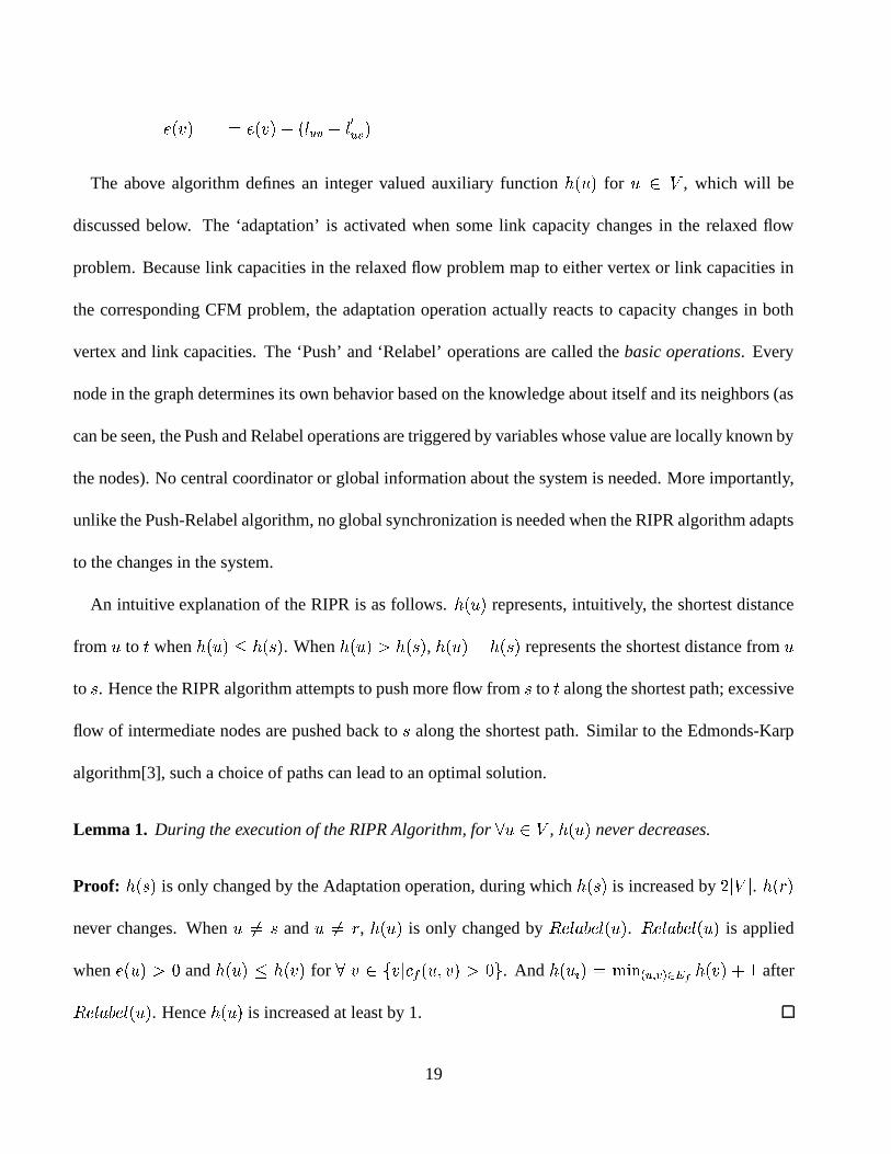
The above algorithm defines an integer valued auxiliary function� � � � for � � �

, which will be

discussed below. The ‘adaptation’ is activated when some link capacity changes in the relaxed flow

problem. Because link capacities in the relaxed flow problem map to either vertex or link capacities in

the corresponding CFM problem, the adaptation operation actually reacts to capacity changes in both

vertex and link capacities. The ‘Push’ and ‘Relabel’ operations are called the basic operations. Every

node in the graph determines its own behavior based on the knowledge about itself and its neighbors (as

can be seen, the Push and Relabel operations are triggered by variables whose value are locally known by

the nodes). No central coordinator or global information about the system is needed. More importantly,

unlike the Push-Relabel algorithm, no global synchronization is needed when the RIPR algorithm adapts

to the changes in the system.

An intuitive explanation of the RIPR is as follows.� � � � represents, intuitively, the shortest distance

from � to&

when� � � � � � � � � . When

� � � � � � � � � , � � � � � � � � � represents the shortest distance from �

to � . Hence the RIPR algorithm attempts to push more flow from � to&

along the shortest path; excessive

flow of intermediate nodes are pushed back to � along the shortest path. Similar to the Edmonds-Karp

algorithm[3], such a choice of paths can lead to an optimal solution.

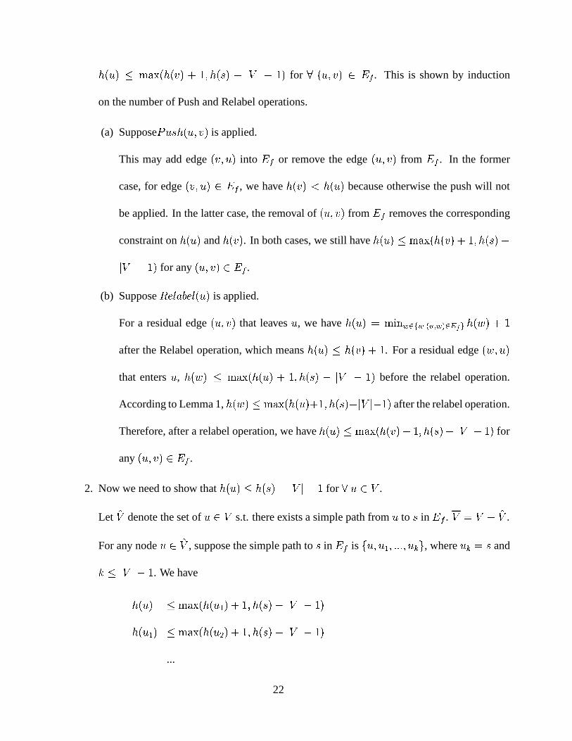
Lemma 1. During the execution of the RIPR Algorithm, for � � � � ,� � � � never decreases.

Proof:� � � � is only changed by the Adaptation operation, during which

� � � � is increased by��

.� � � �

never changes. When � 5 � and � 5 � , � � � � is only changed by � � � � # � � � � � . � � � � # � � � � � is applied

when �� and

� � � � � � � � �for � � � � � 4�� . And

� � �� after

� � � � # � � � � � . Hence� � � � is increased at least by 1.

19

Lemma 2. During the execution of the RIPR Algorithm, for � � � �s.t.

�� , there exists a simple path in

�� from � to a node

�s.t. �

�� .

Proof: Suppose �� . Let

��denotes the set of nodes that can be reached by � through a simple

path in�� . Note that � � ��

. For sake of contradiction, suppose �� for � ��

. Let� � � ��

.

We claim that if ��

and ��

, then� � � � � � � � . Otherwise if

� � � � � � � � , then 4 � � � � � � 4�� 4�� , which means � can be reached from � in

�� , hence there exists a

path from � to � in�� . But this contradicts the choice that �

� �.

It is fairly easy to show that � �� . Hence � �� . But this

contradicts the assumption that �� for � ��

and �� .

Lemma 3. During the execution of the RIPR, for � � � �, if � � � � � � , then either � � � � # � � � � � , or

� � � � � � �� (where� � �

) can be applied.

Proof: When �� , if �

�s.t. 4 � � � �� and

� � � � � � � � �, then � � � � � � �� can be applied;

otherwise,� � � � � � � � �

for � �� 4 � � � �� , which means � � � � # � � � � � can be applied.

Lemma 4. During the execution of the RIPR algorithm,

� � � � � ��

� ��

��

for � � � �� ,� � � � � � � � � � ��

� for � � � �

Proof: We prove by induction on the number of adaptation operations.

� Base case:

Before any changes occur in the system, the adaptation operation will not be applied. At this

stage, the Incremental Push-Relabel algorithm performs the exact operations as the Push-Relabel

algorithm, hence we have

20

� � � � � ��

� ��

��

for � � � � � � � � � ,� � � � � � � � � � ��

� for � � � �

before any adaptation operation is applied.

� Induction step:

Suppose after the adaptation has been applied� �

� times and we still have

� � � � � ��

� ��

��

for � � � � � � � � � ,� � � � � � � � � � ��

� for � � � �

and then the� ��

adaptation,� � �� & � &'$�� , is applied.

1. We first show that� � � � � ��

� � �� for � � � �� after

� � �� & � &'$� � � � � �� .Considering

� � �� & � &'$�� , if either scenario (a) or (c) occurs, no residual edge is added

or removed, no node � � � has its� � � � changed, either. If scenario (d) occurs, the change

in the system removes� � � �� from

� � and hence the corresponding constraint on� � � � �

and� ��

. If scenario (b) occurs,� � � �� is added to the

� � . By induction assumption,

� � � � � � � � � � � �� before the adaptation operation. Because

� � � � � does not change

and� � � � increases by

� �� after the operation,

� � � � � � � � � � � �� after the adaption

operation. In summary, after the adaptation operation,� � � � � �

� � ��

for � � � �� .� � �� & � &'$� � � � � � � � � changes the values of some � � � � , allowing new Push and Relabel opera-

tions to be applied. Yet these operations preserve the property that

21

� � � ��

� ��

��

for � � � � � � � �� . This is shown by induction

on the number of Push and Relabel operations.

(a) Suppose � � � � � � � � � is applied.

This may add edge�� into

�� or remove the edge

� � �� from�� . In the former

case, for edge��

� , we have� �� because otherwise the push will not

be applied. In the latter case, the removal of� � �� from

�� removes the corresponding

constraint on� � � � and

� �� . In both cases, we still have

� � � � � ��

� ��

��

for any� � �� .

(b) Suppose � � � � # � � � � � is applied.

For a residual edge� � �� that leaves � , we have

� � � � �� after the Relabel operation, which means

� � � � � � �� . For a residual edge

� � � � �

that enters � ,� � � � � ��

� � � � � � � � � � � ��

before the relabel operation.

According to Lemma 1,� � � � � ��

� � � � � � � � � � � � � �� after the relabel operation.

Therefore, after a relabel operation, we have� � � � � ��

� � ��

��

for

any� � �� .

2. Now we need to show that� � � � � � � � � � ��

� for � � � � .

Let��

denote the set of � � � s.t. there exists a simple path from � to � in� � . � � � ��

.

For any node � � ��, suppose the simple path to � in

� � is � � � � � � * * * � � � , where � � and

� � �� . We have

� � � � � ��

��

� � � � � � ��

��

...

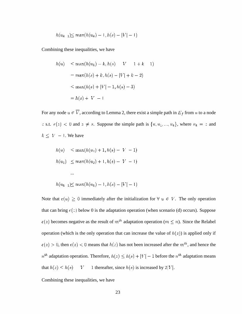
22

� � � � � � � ��

��

Combining these inequalities, we have

� � � � ��

� � � � � � � � � � � � � ��

��

� � � � �

��

� � � � � � ��

� � � � � ��

For any node � � � , according to Lemma 2, there exist a simple path in� � from � to a node

� s.t. �� and � 5 � . Suppose the simple path is � � � �� * * * � � � , where � � and

� � �� . We have

� � � � � ��

��

� � � � � � ��

��

...

� � � � � � � ��

��

Note that � � � � � immediately after the initialization for � � � �. The only operation

that can bring �� below 0 is the adaptation operation (when scenario (d) occurs). Suppose

� � � � becomes negative as the result of/ ��

adaptation operation (/ � �

). Since the Relabel

operation (which is the only operation that can increase the value of� � � � ) is applied only if

� � � � � � , then � � � � � means that� � � � has not been increased after the

/ ��, and hence the

� ��adaptation operation. Therefore,

� � � � � � � � � � �� before the

� ��adaptation means

that� � � � � � � � � � ��

� thereafter, since� � � � is increased by

� �� .

Combining these inequalities, we have

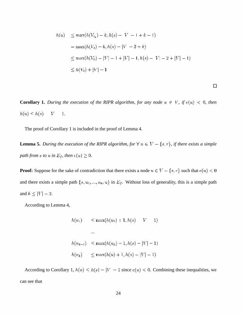
23

� � � � ��

� � � ��

� � � � � �

��

� � � � � � � � ��

��

� � � ��

��

� ��

��

� � � ��

�

Corollary 1. During the execution of the RIPR algorithm, for any node � � �, if �

� � � � , then

� � � � � � � � � � �� .

The proof of Corollary 1 is included in the proof of Lemma 4.

Lemma 5. During the execution of the RIPR algorithm, for �� , if there exists a simple

path from � to � in� � , then � � � � � .

Proof: Suppose for the sake of contradiction that there exists a node � � � � �� such that ��

and there exists a simple path �� * * * � � � � � in� � . Without loss of generality, this is a simple path

and � � �� .

According to Lemma 4,

� � ��

��

...

� � � � � � � ��

��

� � � � � ��

��

According to Corollary 1,� � � � � � � � ��

� since � � � � � . Combining these inequalities, we

can see that

24

� � ��

� � � � � � � � � � � � � ��

��

� � � � � � ��

� � �

� � � � � � ��

��

� � � �

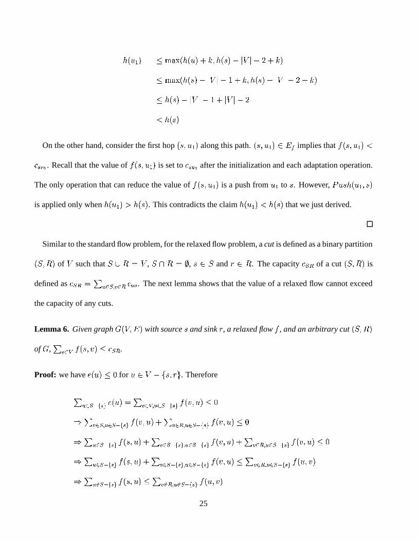
On the other hand, consider the first hop� � � �� along this path.

� � � �� implies that� � � � ��

4 � �� . Recall that the value of� � � � �� is set to 4 � �� after the initialization and each adaptation operation.

The only operation that can reduce the value of� � � � � � � is a push from �� to � . However, � � � � � ��

is applied only when� � �� . This contradicts the claim

� � �� that we just derived.

Similar to the standard flow problem, for the relaxed flow problem, a cut is defined as a binary partition

� � � � � of�

such that��

,��

, � � � and � � � . The capacity 4�� of a cut� � � � � is

defined as 4�� 4 �� . The next lemma shows that the value of a relaxed flow cannot exceed

the capacity of any cuts.

Lemma 6. Given graph � � � � � � with source � and sink � , a relaxed flow�

, and an arbitrary cut� � � � �

of � , � �� 4�� .

Proof: we have � � � � � � for � � � � �� . Therefore

� � ��

25

� � � ��

Since� � � �� 4 �� for � � �� , additionally, because

� � � � � � )� , we have

� �� 4 � � )4 ��

The next lemma shows that the RIPR algorithm finds the maximum relaxed flow if it terminates. After

proving this lemma, we will show that the RIPR algorithm indeed terminates.

Lemma 7. If the RIPR algorithm terminates, it finds the maximum relaxed flow.

Proof:

According to Lemma 3, if the algorithm terminates, then �� for �� . Hence

�is

a flow if the algorithm terminates.

Given such an�

, we construct a cut of � as follows:

� � � � ��

� � � �

According to Lemma 5, �� for � � � � �� . Note that �

� � � � � for �� upon

termination of the algorithm. Hence � � � � � (i.e. � �� ) for � � � � � �� . Then it is

easy to show that � � �� .Therefore,

� ��

26

� � ��

� � ��

We claim that� � � �� 34 �� for �� , because otherwise

� � � �� 4 �� implies that edge

� � �� , hence�

can be reached by � in�� . But this contradicts the definition of � .

Therefore,

� �� 4 � � �� )4 ��

According to Lemma 6, such a relaxed flow�

is a maximum relaxed flow.

Now we show that the algorithm indeed terminates.

Lemma 8. If the adaptation is applied�

(� � ) times, then the number of Relabel operations that can

be performed is less than� � ��

.

Proof: If the adaptation is applied�

times, then� � � � � � �

� ��

. According to Lemma 4,� � � � �

� � � � � ��

��

� for �� . Each time � � � � # � � � � � is applied,

� � � � is increased at

least by 1. Since� � � � )� initially, � � � � # � � � � � is applied at most

� � ��

� times. There are ��

nodes in the system, hence then the total number of Relabel operations that can be performed is at most

� � � ��

��

, which is less than� � ��

.

If a � � � � � � �� operation removes� � �� from

� � (i.e. 4�� after the operation), it is a

saturated push, otherwise it is a non-saturated push.


(�� ) times, then the number of saturated push operations

that can be performed is less than��

� �� .

Proof: Consider edge� � ��

. Suppose a saturated push � � � � � � �� is first applied. For a second

saturated push to be applied over� � �� , � � � � �� must be applied before the second saturated push.

27

Because� � � � � � ��

for the first push (otherwise the first push will not be applied), then� ��

must

be increased at least by 2, otherwise� �� then � � � � � �� will not be applied. Similarly,

� � � �

must be increased at least by 2 for the second saturated push to occur over edge� � �� . So on so force.

Because� � � � � � � � � � ��

��

� ,� � � � and

� � � �cannot increase to infinity. It is easy

to show that saturated push can occur at most� � � �

��

�� ! �

times for edge� � �� . There are

��

edges in the graph. The total number of saturated push operations is less than� � � �

��

��.!��

,

which is less than��

� �� .


(� � ) times, then the number of non-saturated push opera-

tions that can be performed is less than� � ��

� � ��

.

Proof: Define a potential function �� . � �� initially. Obviously, � � .

According to Lemma 4,� � � � � � � � � � ��

��

� , hence a relabel operation increases �

by at most� � ��

� . According to Lemma 8, there can be at most� � ��

Relabel operations.

The increase in � induced by all relabel operations is at most� � � �

��

��

��

. A saturated

push � � � � � � �� increases � by at most� � ��

� since ��

may become positive after the push,

and� � �

��

� is the highest value that� � � �

can be. According to Lemma 9, the increase in �

induced by all saturated push is at most� � � �

��

��

� ��

.

For a non-saturated push � � � � � � �� , � � � � � � before the push and � � � � � after the push, hence

� � � � is excluded from � after the push. If � �� after the push, � is decreased at least by 1 because

� � � � � � � � � � � . If � �� after the push, then � is decreased by� � � � � .

Therefore, the total increase in � is at most� � � �

��

��

��

��

��

��

� � ��

� ��

� � ��

, while each non-saturated push decreases �

at least by 1. Therefore, the total number of non-saturated push operations that can be performed is at

28

most� � ��

� � ��

.

Theorem 2. The RIPR algorithm finds the maximum flow for the relaxed flow problem with

� � � � �� basic operations, where

�is the number of adaptation operations performed,

��

is the number of nodes in the graph, and ��

is the number of edges in the graph.

Proof: Immediate from Lemma 7, 8, 9, and 10.

4.3 A Simple Protocol for Data Gathering

In this section, we present a simple on-line protocol for SMaxDT problem based on the RIPR algo-

rithm in Section 4.

In this protocol, each node maintains a data buffer. Initially, all the data buffers are empty. The source

node � senses the environment and fills its buffer continuously. At any time instance, let � � denote the

amount of buffer used by node � . Each node � � � operates as follows:

1. Contact the adjacent node(s) and execute the RIPR algorithm.

2. While � � � � , send message ‘request to send’ to all successors�

of � s.t.� � � � � � � � . If ‘clear

to send’ is received from�, then set �� and send a data packet to

�at rate

� � � �� .(recall that

� � � �� is the flow rate at which data should be sent from � to�

according to the RIPR

algorithm.)

3. Upon receiving ‘request to send’, � acknowledges ‘clear to send’ if � � �� . Here�

is a pre-set

threshold that limits the maximum number of data packets a buffer can hold.

For node � , it stops sensing if � � �� . The nodes execute the RIPR algorithm and find the rate� � � ��

for sending the data. Meanwhile, the nodes transfer the data according to the values of� � � �� , without

29

waiting for the RIPR algorithm to terminate. Two types of data are transferred in the system: the control

messages that are used by the RIPR algorithm, and the sensed data themselves. The control messages are

exchanged among the nodes to query and update the values of� � � �� and

� � when executing the RIPR

algorithm. The control messages and the sensed data are transmitted over the same links and higher

priority is given to the control messages in case of a conflict.

For the MMaxDT problem, the situation is a bit more complicated. Since the MMaxDT problem is

reduced to the SMaxDT problem by adding a hypothetical super source node � � , the RIPR algorithm

needs to maintain the flow out of � � as well as the value of function� � � � � . Additionally, the values of

� � � � � � � (��

) and� � � � � are needed by all nodes � � �� during the execution of the algorithm. Because

� � is not an actual sensor, sensors in��

therefore need to maintain a consistent image of � � . This requires

some regional coordination among sensors in��

and may require some extra cost to actually implement

such a consistent image.

The SMaxDV and MMaxDV problems are by nature off-line problems and we do not develop online

protocols for the two problems.

5 Experimental Results

Simulations were conducted to illustrate the effectiveness of the RIPR algorithm and the data gather-

ing protocol. For the sake of illustration, we present simulation results for the SMaxDT problem.

The systems were generated by randomly scattering the sensor nodes in a unit square. The base station

was located at the lower-left corner of the square. The source node was randomly chosen from the sensor

nodes. 8 � ’s are uniformly distributed between 0 and 8 �,� � . 8 �,� � was set to 100. We assume a signal

decaying factor of � � . The flow capacity between sensor nodes � and�

is determined by Shannon’s

30

theorem as � �� where � is the bandwidth of the link, � � � is the distance between

� and�, � � � is the transmission power on link

� � �� , and � is the noise in the communication channel.

In all the simulations, � was set to �� , � �� was set to � � � � / � , and � was set to � � �� / � .�

was

set to 2. Each data packet was assumed to contain 32 bytes. Each control message was assumed to be

transferred in 1/ � .

The RIPR algorithm described in Section 4 adapts to every single change that occurs in the system.

The adaptation is initiated by source node � , which increases� � � � by

� �� and pushes flow to every

node in � � . However, the adaptation can be performed in batch mode, i.e. source node � initiates the

adaptation after multiple changes have occurred in the system. Since the proof of Theorem 2 does not

utilize any information about the number of changes occurred, the correctness and complexity of the

RIPR algorithm still holds even if the adaptation is performed in batch mode. We have observed that the

RIPR algorithm always finds the optimal solution, regardless of the number of changes occurred before

the adaptation is performed.

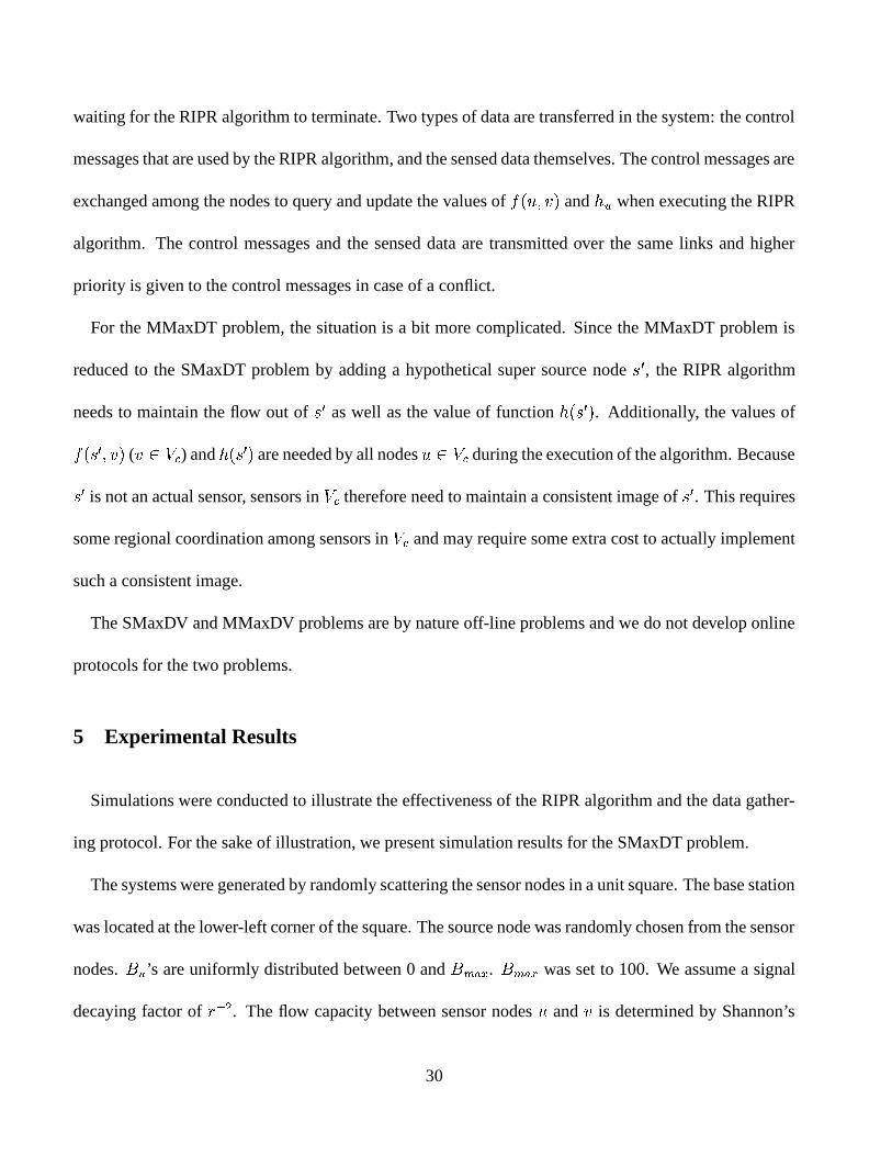
The result in Figure 2 illustrates the cost of adaptation (in terms of the total number of basic op-

erations) vs the number of changes occurred before the adaptation. In each experiment, a randomly

generated system with 40 nodes was deployed in a unit square. After the system stabilized and found

the optimal solution, the bandwidth of a certain number of links was changed. Then adaptation was

performed and the system stabilized again (and found a new optimal solution) after executing a certain

number of basic operations. For each experiment, we record the number of basic operations executed

by the system to find the new optimal solution. Each data point in Figure 2 is averaged over 50 experi-

ments. We can see that the required number of basic operations increases as the number of changes (per

adaptation) increases.

31

0 50 100 1500

100

200

300

400

500

600

700

Number of changes in the systemN

umbe

r of

bas

ic o

pera

tions

Figure 2. Adaptation performed in batch mode

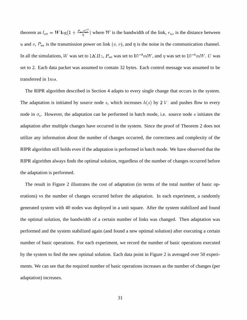
So far the performance of the RIPR algorithm is evaluated in terms of the total number of basic

operations. We do not expect the individual nodes to execute the same number of operations since the

RIPR algorithm is not designed for load balancing. But interestingly, the following simulation results

show that the RIPR algorithm is pretty well-balanced in terms of the number of basic operations executed

by different nodes. For each experiment, a randomly generated system is initialized and the number

of basic operations executed by the system to stabilize was recorded. The basic operations were re-

classified into two categories: local updates and control message exchanges. Each push� � � � � operation

consists of one local update at � , one message transfer (send) at � , and one message transfer (receive) at

�. Each relabel

� � � operation consists of one local update at � , one message transfer (broadcast� � � � to

� � ) at � , and one message transfer (receive� � � � ) at each

� � � � . Figure 3 shows the number of local

updates and control message executed/transferred by the nodes. We report the maximum and the mean

number of local updates, and the maximum and mean number of control message exchanges. Each data

point is averaged over 100 experiments. Figure 3 shows that the maximum number of local updates

is only about 2 times the mean number of local updates. The maximum number of control message

exchanges is also about 2 times the mean number of control message exchanges. This result shows that

32

50 100 150 2000

2000

4000

6000

8000

10000

12000

14000

16000

Number of nodesN

umbe

r of

bas

ic o

pera

tions

Max ctrl Mean ctrl Max update Mean update

Figure 3. The maximum and mean cost per node for executing the RIPR algorithm

the RIPR algorithm is quite well-balanced in terms of per node cost.

The second set of simulation results illustrate the convergence and adaptivity of the proposed protocol.

In each experiment, a certain number (between 40 and 100) of nodes were randomly deployed in the unit

square. Communication radius ranging from 0.2 to 0.5 units were tested. For each experiment, the data

gathering process lasted 30 seconds.

The steady state throughput is calculated as the average throughput during the last 10 seconds of data

gathering. Table 1 shows the steady state throughput of the protocol. The results have been normalized

to the optimal throughput. The optimal throughput was calculated offline. Each data point in Table 1 is

averaged over 50 systems. The results show that the steady state throughput of the proposed protocol

approaches the optimal throughput, regardless of the number of nodes and the communication radius.

In the protocol, data is transferred when the RIPR algorithm is being executed. Hence the start-up

time of the system needs to be evaluated from two aspects: the execution time of the RIPR algorithm

(i.e. how fast the RIPR algorithm terminates), and the time for the data transfer to reach steady state

throughput.

For each experiment in the second set of simulations, we monitored the activities of each individual

33

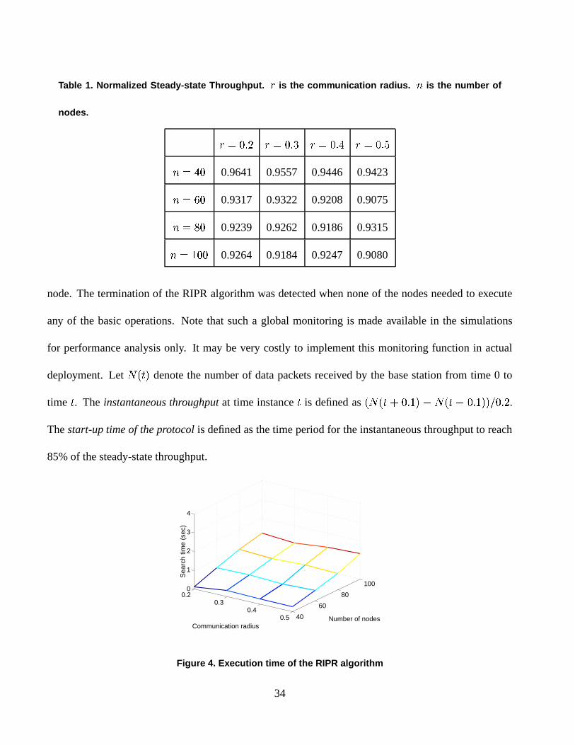
Table 1. Normalized Steady-state Throughput. � is the communication radius.�

is the number of

nodes.

� �+* � � �� * � � )�+* � � )� * �� 0.9641 0.9557 0.9446 0.9423

� �� 0.9317 0.9322 0.9208 0.9075

� �� 0.9239 0.9262 0.9186 0.9315

� � � � 0.9264 0.9184 0.9247 0.9080

node. The termination of the RIPR algorithm was detected when none of the nodes needed to execute

any of the basic operations. Note that such a global monitoring is made available in the simulations

for performance analysis only. It may be very costly to implement this monitoring function in actual

deployment. Let �� & �

denote the number of data packets received by the base station from time 0 to

time&. The instantaneous throughput at time instance

&is defined as

�� &��+* � � � � � & � �+* � � �.! �+* � .

The start-up time of the protocol is defined as the time period for the instantaneous throughput to reach

85% of the steady-state throughput.

0.20.3

0.40.5 40

60

80

1000

1

2

3

4

Number of nodesCommunication radius

Sea

rch

time

(sec

)

Figure 4. Execution time of the RIPR algorithm

34

0.20.3

0.40.5 40

60

80

100

0

1

2

3

4

Number of nodesCommunication radius

Sta

rt−

up ti

me

(sec

)

Figure 5. Start-up time of the proposed protocol

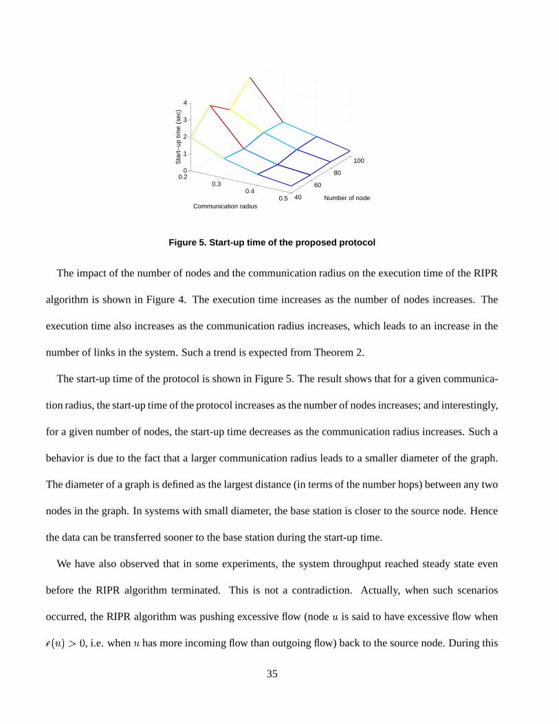
The impact of the number of nodes and the communication radius on the execution time of the RIPR

algorithm is shown in Figure 4. The execution time increases as the number of nodes increases. The

execution time also increases as the communication radius increases, which leads to an increase in the

number of links in the system. Such a trend is expected from Theorem 2.

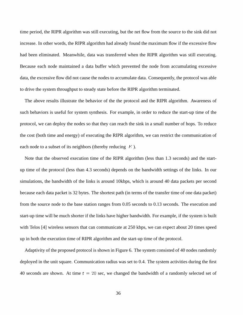
The start-up time of the protocol is shown in Figure 5. The result shows that for a given communica-

tion radius, the start-up time of the protocol increases as the number of nodes increases; and interestingly,

for a given number of nodes, the start-up time decreases as the communication radius increases. Such a

behavior is due to the fact that a larger communication radius leads to a smaller diameter of the graph.

The diameter of a graph is defined as the largest distance (in terms of the number hops) between any two

nodes in the graph. In systems with small diameter, the base station is closer to the source node. Hence

the data can be transferred sooner to the base station during the start-up time.

We have also observed that in some experiments, the system throughput reached steady state even

before the RIPR algorithm terminated. This is not a contradiction. Actually, when such scenarios

occurred, the RIPR algorithm was pushing excessive flow (node � is said to have excessive flow when

� � � � � � , i.e. when � has more incoming flow than outgoing flow) back to the source node. During this

35

time period, the RIPR algorithm was still executing, but the net flow from the source to the sink did not

increase. In other words, the RIPR algorithm had already found the maximum flow if the excessive flow

had been eliminated. Meanwhile, data was transferred when the RIPR algorithm was still executing.

Because each node maintained a data buffer which prevented the node from accumulating excessive

data, the excessive flow did not cause the nodes to accumulate data. Consequently, the protocol was able

to drive the system throughput to steady state before the RIPR algorithm terminated.

The above results illustrate the behavior of the the protocol and the RIPR algorithm. Awareness of

such behaviors is useful for system synthesis. For example, in order to reduce the start-up time of the

protocol, we can deploy the nodes so that they can reach the sink in a small number of hops. To reduce

the cost (both time and energy) of executing the RIPR algorithm, we can restrict the communication of

each node to a subset of its neighbors (thereby reducing ��

).

Note that the observed execution time of the RIPR algorithm (less than 1.3 seconds) and the start-

up time of the protocol (less than 4.3 seconds) depends on the bandwidth settings of the links. In our

simulations, the bandwidth of the links is around 10kbps, which is around 40 data packets per second

because each data packet is 32 bytes. The shortest path (in terms of the transfer time of one data packet)

from the source node to the base station ranges from 0.05 seconds to 0.13 seconds. The execution and

start-up time will be much shorter if the links have higher bandwidth. For example, if the system is built

with Telos [4] wireless sensors that can communicate at 250 kbps, we can expect about 20 times speed

up in both the execution time of RIPR algorithm and the start-up time of the protocol.

Adaptivity of the proposed protocol is shown in Figure 6. The system consisted of 40 nodes randomly

deployed in the unit square. Communication radius was set to 0.4. The system activities during the first

40 seconds are shown. At time& � � sec, we changed the bandwidth of a randomly selected set of

36

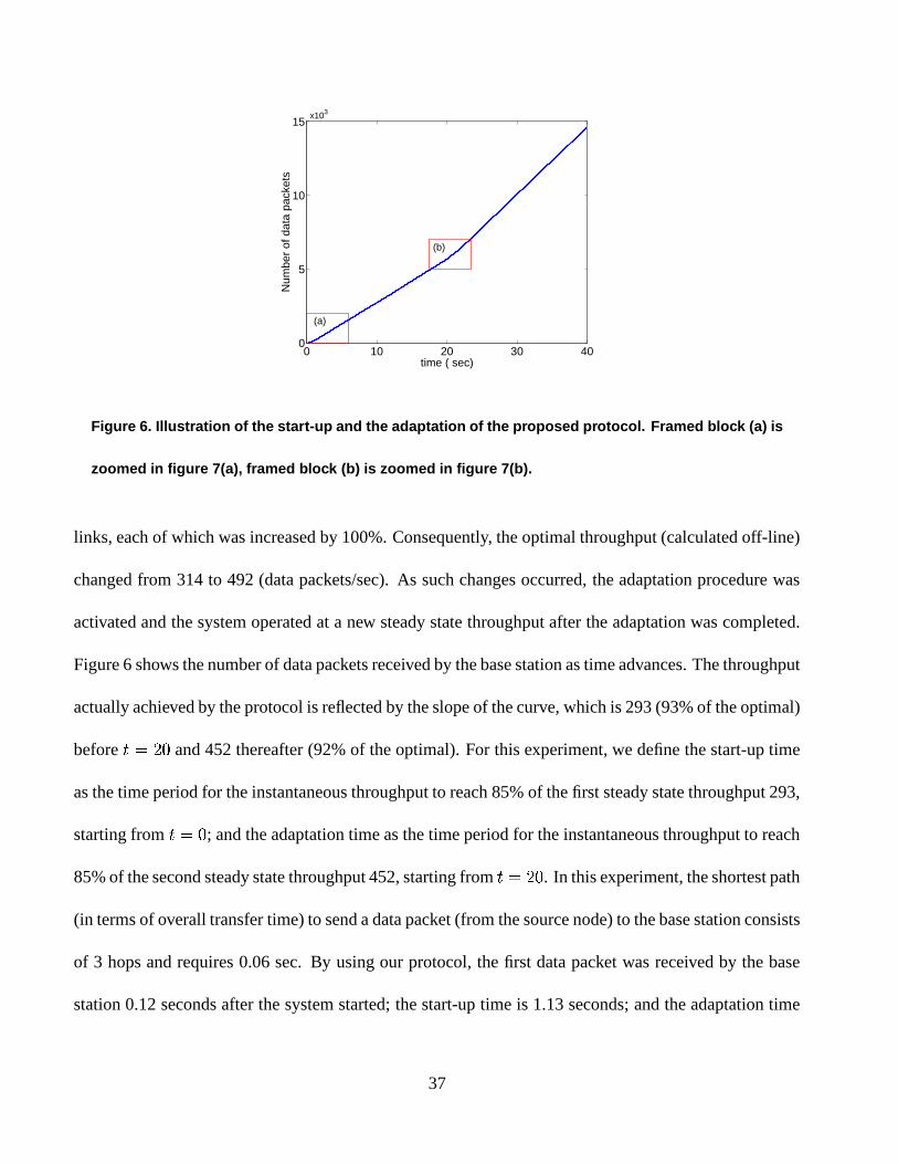
0 10 20 30 400

5

10

15 x103

time ( sec)

Num

ber

of d

ata

pack

ets

(b)

(a)

Figure 6. Illustration of the start-up and the adaptation of the proposed protocol. Framed block (a) is

zoomed in figure 7(a), framed block (b) is zoomed in figure 7(b).

links, each of which was increased by 100%. Consequently, the optimal throughput (calculated off-line)

changed from 314 to 492 (data packets/sec). As such changes occurred, the adaptation procedure was

activated and the system operated at a new steady state throughput after the adaptation was completed.

Figure 6 shows the number of data packets received by the base station as time advances. The throughput

actually achieved by the protocol is reflected by the slope of the curve, which is 293 (93% of the optimal)

before& � � and 452 thereafter (92% of the optimal). For this experiment, we define the start-up time

as the time period for the instantaneous throughput to reach 85% of the first steady state throughput 293,

starting from& �� ; and the adaptation time as the time period for the instantaneous throughput to reach

85% of the second steady state throughput 452, starting from& � � . In this experiment, the shortest path

(in terms of overall transfer time) to send a data packet (from the source node) to the base station consists

of 3 hops and requires 0.06 sec. By using our protocol, the first data packet was received by the base

station 0.12 seconds after the system started; the start-up time is 1.13 seconds; and the adaptation time

37

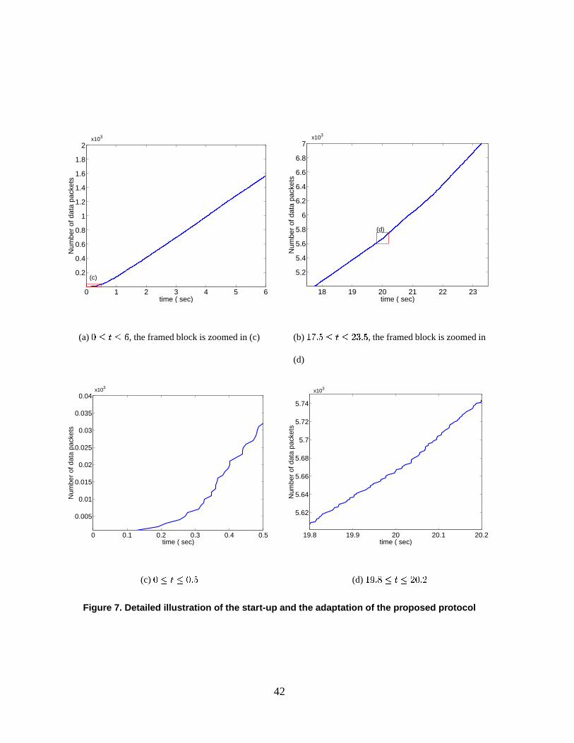
is 1.4 seconds. The system activities during the start-up and adaptation period are shown in more detail

in Figure 7. An important observation from Figure 7 is that the system started (at& � ) and continued

(at& � � ) to gather data while the RIPR algorithm was still executing. The system did not wait until

the optimal solution was found. Actually, because the protocol was executed in a distributed fashion,

none of the nodes would know the completion of the RIPR algorithm unless a global synchronization

was performed.

6 Conclusion

In this paper, we studied a set of data gathering problems in energy-constrained networked sensor

systems. We reduced such problems to a network flow maximization problem with vertex capacity

constraint, which can be further reduced to the standard network flow problem. After deriving a relaxed

formulation for the standard network problem, we developed a distributed and adaptive algorithm to

maximize the flow. This algorithm can be approximated as a simple data gathering protocol.

One of the future directions is to design distributed algorithms that do not generate excessive flow at

the nodes (i.e. � � � � does not become positive) during the execution. Our formulation of constrained

flow optimizations can be applied to problems beyond the four problems discussed in this paper. For

example, the system model considered in [11] gathers data in rounds. In each round, every sensor

generates one data packet and the data packets from all the sensors need to be collected by the sink. The

goal is to maximize the total number of rounds the system can operate under energy constraints on the

nodes. This problem can be described by our constrained flow formulation and an optimal solution can

be developed [10].

38

References

[1] I. F. Akyildiz, W. Su, Y. Sankarasubramaniam, and E. Cyirci. Wireless Sensor Networks: A Survey.

Computer Networks, 38(4):393–422, 2002.

[2] G. Asada, T. Dong, F. Lin, G. Pottie, W. Kaiser, and H. Marcy. Wireless Integrated Network Sen-

sors: Low Power Systems on a Chip. In Proceedings of European Solid State Circuits Conference,

1998.

[3] T. H. Cormen, C. E. Leiserson, and R. L. Rivest. Introduction to Algorithms. MIT Press, 1992.

[4] Moteiv Corporation. Telos Wireless Sensor Module. http://www.moteiv.com.

[5] C. Efthymiou, S. Nikoletseas, and J. Rolim. Energy Balanced Data Propagation in Wireless Sensor

Networks. 4th International Workshop on Algorithms for Wireless, Mobile, Ad Hoc and Sensor

Networks (WMAN ’04), hold in conjunction with IPDPS 2004, April 2004.

[6] E. Falck, P. Floreen, P. Kaski, J. Kohonen, and P. Orponen. Balanced Data Gathering in Energy-

Constrained Sensor Networks. In Sotiris Nikoletseas and Jose D. P. Rolim, editors, Algorithmic

Aspects of Wireless Sensor Networks (First International Workshop, ALGOSENSORS 2004), July

2004.

[7] A. V. Goldberg and R. E. Tarjan. A New Approach to the Maximum Flow Problem. Journal of

Association for Computing Machinery, 35:921–940, 1988.

[8] W. B. Heinzelman. An Application-Specific Protocol Architecture for Wireless Microsensor Net-

works. IEEE Transactions on Wireless Communications, 1(3), 2002.

39

[9] W. R. Heinzelman, A. Chandrakasan, and H. Balakrishnan. Energy Efficient Communication Pro-

tocol for Wireless Micro-sensor Networks. In Proceedings of IEEE Hawaii International Confer-

ence on System Sciences, 2000.

[10] B. Hong and V. K. Prasanna. Optimizing System Life time for Data Gathering in Networked Sensor

Systems. AlgorithmS for Wireless and Ad-hoc Networks (A-SWAN 2004) (Held in conjunction with

MobiQuitous 2004), August 2004.

[11] K. Kalpakis, K. Dasgupta, and P. Namjoshi. Maximum Lifetime Data Gathering and Aggregation

in Wireless Sensor Networks. IEEE Networks ’02 Conference, 2002.

[12] E. L. Lawler. Combinatorial Optimization : Networks and Matroids. Holt, Rinehart and Winston,

1976.

[13] R. Min, T. Furrer, and A. Chandrakasan. Dynamic Voltage Scaling Techniques for Distributed

Microsensor Networks. Workshop on VLSI (WVLSI ’00), April 2000.

[14] F. Ordonez and B. Krishnamachari. Optimal Information Extraction in Energy-Limited Wireless

Sensor Networks. to appear in IEEE Journal on Selected Areas in Communications, special issue

on Fundamental Performance Limits of Wireless Sensor Networks, 2004.

[15] J. Rabaey, J. Ammer, T. Karalar, S. Li, B. Otis, M. Sheets, and T. Tuan. PicoRadios for Wire-

less Sensor Networks: The Next Challenge in Ultra-Low-Power Design. In Proceedings of the

International Solid-State Circuits Conference, 2002.

[16] N. Sadagopan and B. Krishnamachari. Maximizing Data Extraction in Energy-Limited Sensor

Networks. IEEE Infocom 2004, 2004.

40

[17] C. Schurgers, O. Aberthorne, and M. Srivastava. Modulation Scaling for Energy Aware Com-

munication Systems. In International Symposium on Low Power Electronics and Design, August

2001.

[18] M. Singh and V. K. Prasanna. Optimal Energy Balanced Algorithm for Selection in Single Hop

Sensor Network. IEEE International Workshop on Sensor Network Protocols and Applications

(SNPA) ICC, 2003.

[19] S. Singh and C. Raghavendra. PAMAS: Power Aware Multi-Access protocol with Signalling for

Ad Hoc Networks. ACM ComputerCommunications Review, 1998.

[20] B. Warneke, M. Last, B. Liebowitz, and K. S. J. Pister. Smart Dust: Communicating with a Cubic-

Millimeter Computer. Computer, 34(1):44–51, 2001.

[21] Y. Yu and V. K. Prasanna. Energy-Balanced Task Allocation for Collaborative Processing in Net-

worked Embedded System. ACM Conference on Language, Compilers, and Tools for Embedded

Systems (LCTES), 2003.

41

0 1 2 3 4 5 6

0.2

0.4

0.6

0.8

1

1.2

1.4

1.6

1.8

2 x103

time ( sec)

Num

ber

of d

ata

pack

ets

(c)

(a) �� , the framed block is zoomed in (c)

18 19 20 21 22 23

5.2

5.4

5.6

5.8

6

6.2

6.4

6.6

6.8

7 x103

time ( sec)N

umbe

r of

dat

a pa

cket

s

(d)

(b) �� , the framed block is zoomed in

(d)

0 0.1 0.2 0.3 0.4 0.5

0.005

0.01

0.015

0.02

0.025

0.03

0.035

0.04 x103

time ( sec)

Num

ber

of d

ata

pack

ets

(c) ��

19.8 19.9 20 20.1 20.2

5.62

5.64

5.66

5.68

5.7

5.72

5.74

x103

time ( sec)

Num

ber

of d

ata

pack

ets

(d) ��

Figure 7. Detailed illustration of the start-up and the adaptation of the proposed protocol

42

Maximum Data Gathering in Networked Sensor Systems

Documents