Max-Plank Institut für Informatik systematic error parallelogram rule polygonal rules exact prediction Geometry Prediction for High Degree Polygons Martin.

Max-Plank Institut für Informatik

systematic error

parallelogram rule

polygonal rules

exact prediction

Geometry Prediction

forHigh Degree

Polygons

Martin Isenburg Stefan Gumhold

Ioannis Ivrissimtzis Hans-Peter Seidel

INFORMATIKINFORMATIK

Compression

• real stuff– sleeping bags

– compressed air

• polygon meshes– faster downloads / less storage

– collaborative CAD

– distribution of simulation results

– archival of spare parts / history

Movies

“Rustboy” animated short by Brian Taylor

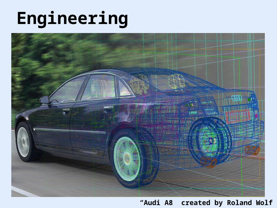
Engineering

“Audi A8” created by Roland Wolf

Architectural Visualization

“Atrium” created by Karol Myszkowski and Frederic Drago

Product Catalogues

“Bedroom set-model Assisi” created by Stolid

Historical Study

scanning of “Michelangelo’s David” courtesy of Marc Levoy

Computer Games

screen shot of “The village of Gnisis”, The Elder Scrolls III

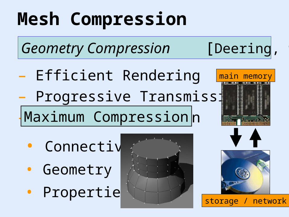
– Efficient Rendering

– Progressive Transmission

– Maximum Compression

• Connectivity

• Geometry

• Properties

Mesh Compression

Geometry Compression [Deering, 95]

storage / network

main memory

Maximum Compression

Most Popular Coder

Triangle Mesh Compression[Touma & Gotsman, 98]

. . . . . .64 4 4 M 5 4S6 6 6

• connectivity with vertex degrees

( )-3-21

( )74-3

( )20-2

. . . . . .( )1-1-1

( )-200

( )-47-2

( )1-21

( )24-1

• geometry with corrective vectors

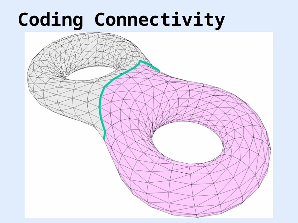
Coding Connectivity

Predicting Geometry

Not Triangles … Polygons!

Face Fixer [Isenburg & Snoeyink, 00]

Coding Polygon Connectivity

Compressing Polygon Mesh Connectivity with Degree Duality … [Isenburg, 02]

same compression in primal and dual !!

Predicting Polygon Geometry

Compressing Polygon Mesh Geometry with Parallelogram … [Isenburg & Alliez, 02]

but … does not work well in the dual !!

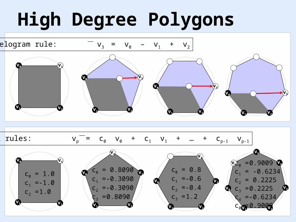
High Degree Polygons

v2v1

v0

v4

v2v1

v0 v3

c0 = 0.8090c1 = -0.3090c2 = -0.3090c3 = 0.8090

c0 = 0.8c1 = -0.6c2 = -0.4c3 = 1.2

v3

v4

c0 = 0.9009c1 = -0.6234c2 = 0.2225c3 = 0.2225c4 = -0.6234c0 = 0.9009v2v1

v0v3

v4

v5

v6

v2v1

v3v0

c0 = 1.0c1 = -1.0c2 = 1.0

polygonal rules: vp = c0 v0 + c1 v1 + … + cp-1 vp-1

v2v1

v2v1

v0v3

v3v0

v2v1

v0v3

v2v1

v0 v3

parallelogram rule: v3 = v0 – v1 + v2

Overview

• Motivation

• Geometry Compression

• Frequency of Polygons

• Polygonal Prediction Rules

• Results

• DiscussionINFORMATIKINFORMATIK

Geometry Compression

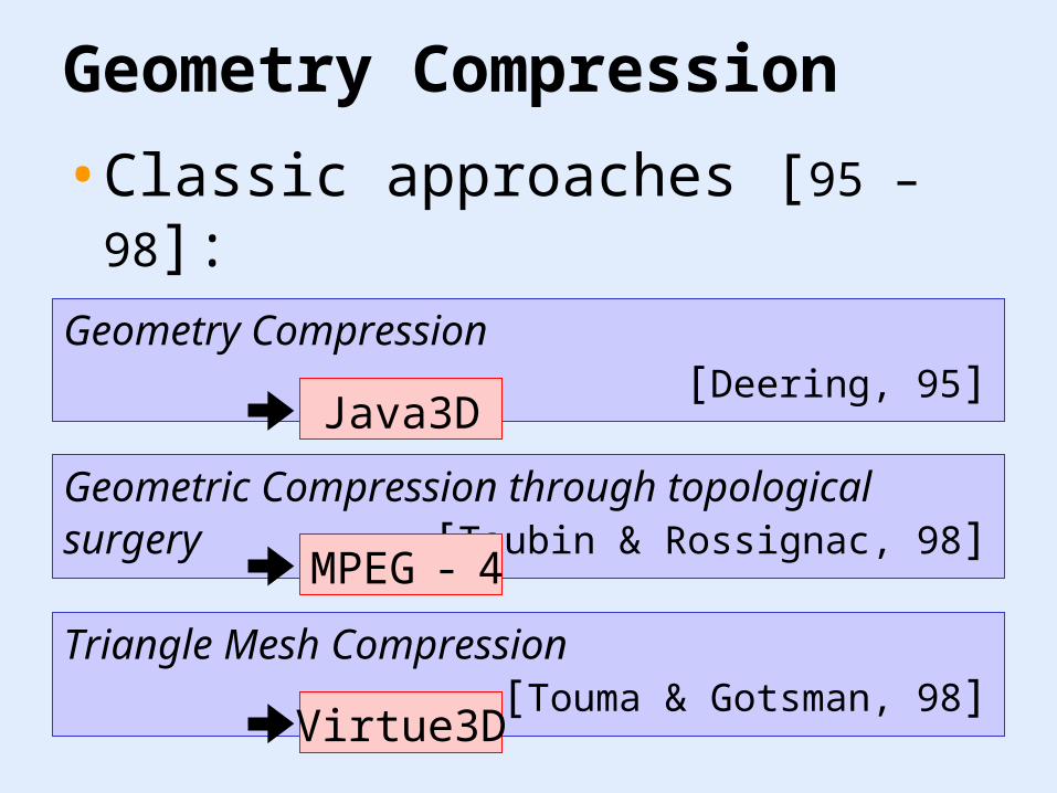
• Classic approaches [95 – 98]:– linear prediction

Geometry Compression[Deering, 95]

Geometric Compression through topological surgery [Taubin & Rossignac, 98]

Triangle Mesh Compression[Touma & Gotsman, 98]

Java3D

MPEG - 4

Virtue3D

Geometry Compression

• Classic approaches [95 – 98]:– linear prediction

• Recent approaches [00 – 03]:– spectral

– re-meshing

– space-dividing

– vector-quantization

– angle-based

– delta coordinates

Geometry Compression

• Classic approaches [95 – 98]:– linear prediction

• Recent approaches [00 – 03]:– spectral

– re-meshing

– space-dividing

– vector-quantization

– angle-based

– delta coordinates

Spectral Compressionof Mesh Geometry

[Karni & Gotsman, 00]

expensive numericalcomputations

Geometry Compression

• Classic approaches [95 – 98]:– linear prediction

• Recent approaches [00 – 03]:– spectral

– re-meshing

– space-dividing

– vector-quantization

– angle-based

– delta coordinates

Progressive GeometryCompression

[Khodakovsky et al., 00]

modifies mesh priorto compression

Geometry Compression

• Classic approaches [95 – 98]:– linear prediction

• Recent approaches [00 – 03]:– spectral

– re-meshing

– space-dividing

– vector-quantization

– angle-based

– delta coordinates

Geometric Compressionfor interactive transmission

[Devillers & Gandoin, 00]

poly-soups; complexgeometric algorithms

Geometry Compression

• Classic approaches [95 – 98]:– linear prediction

• Recent approaches [00 – 03]:– spectral

– re-meshing

– space-dividing

– vector-quantization

– angle-based

– delta coordinates

Vertex data compressionfor triangle meshes

[Lee & Ko, 00]

local coord-system +vector-quantization

Geometry Compression

• Classic approaches [95 – 98]:– linear prediction

• Recent approaches [00 – 03]:– spectral

– re-meshing

– space-dividing

– vector-quantization

– angle-based

– delta coordinates

Angle-Analyzer: A triangle-quad mesh codec

[Lee, Alliez & Desbrun, 02]

dihedral + internal =heavy trigonometry

Geometry Compression

• Classic approaches [95 – 98]:– linear prediction

• Recent approaches [00 – 03]:– spectral

– re-meshing

– space-dividing

– vector-quantization

– angle-based

– delta coordinates

High-Pass Quantization forMesh Encoding

[Sorkine et al., 03]

basis transformationwith Laplacian matrix

Linear Prediction Schemes

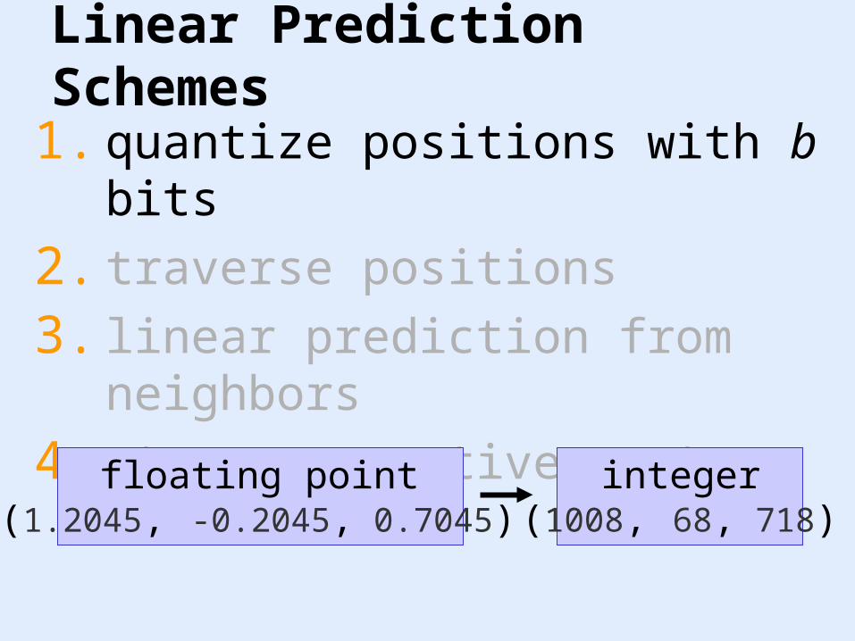
1. quantize positions with b bits

2. traverse positions

3. linear prediction from neighbors

4. store corrective vector

(1.2045, -0.2045, 0.7045) (1008, 68, 718)floating point integer

Linear Prediction Schemes

1. quantize positions with b bits

2. traverse positions

3. linear prediction from neighbors

4. store corrective vector

use traversal order implied bythe connectivity coder

Linear Prediction Schemes

1. quantize positions with b bits

2. traverse positions

3. linear prediction from neighbors

4. store corrective vector

(1004, 71, 723)apply prediction rule prediction

Linear Prediction Schemes

1. quantize positions with b bits

2. traverse positions

3. linear prediction from neighbors

4. store corrective vector0

10

20

30

40

50

60

70

position distribution

0

500

1000

1500

2000

2500

3000

3500

corrector distribution

(1004, 71, 723)(1008, 68, 718)position

(4, -3, -5)correctorprediction

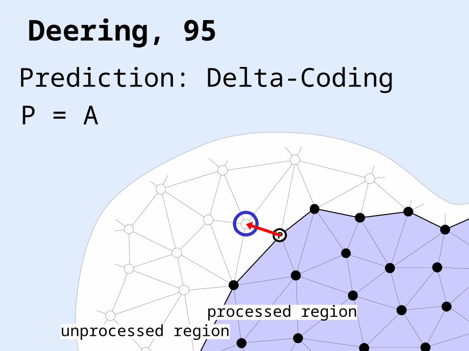
Deering, 95

Prediction: Delta-Coding

A

processed regionunprocessed region

P

P = A

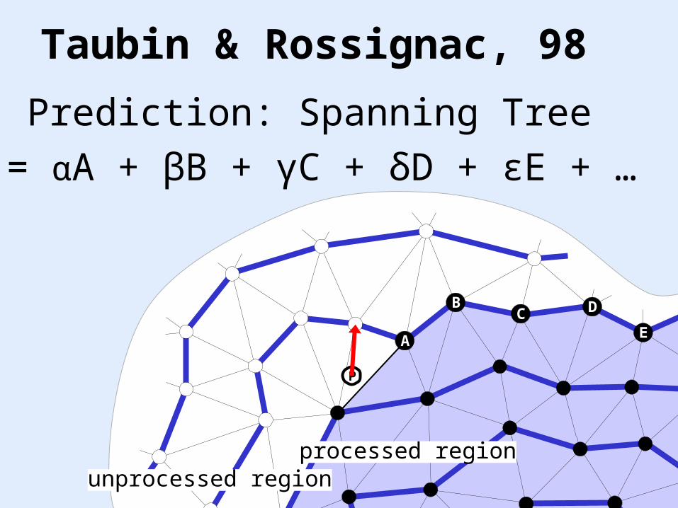
Taubin & Rossignac, 98

Prediction: Spanning Tree

A

BC D

E

processed regionunprocessed region

P

P = αA + βB + γC + δD + εE + …

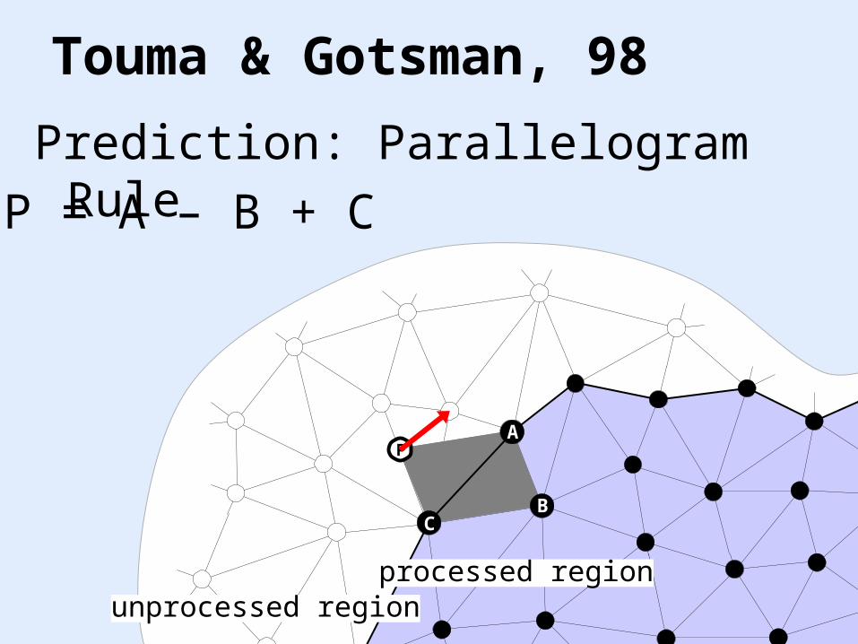
Touma & Gotsman, 98

Prediction: Parallelogram Rule

processed regionunprocessed region

P

P = A – B + C

A

BC

“within”- predictions often find existing parallelograms (i.e. quadrilateral faces)

“within” versus “across”

“within”- predictions avoid creases

within-predictionacross-prediction

Overview

• Motivation

• Geometry Compression

• Frequency of Polygons

• Polygonal Prediction Rules

• Results

• DiscussionINFORMATIKINFORMATIK

Discrete Fourier Transform (1)

)1)(1()1(21

)1(242

12

1

1

1

1111

1F

nnnn

n

n

n

nn CC

ni /2e where .

The Discrete Fourier Transform (DFT) of a complex vector is a basis transform that is described by the matrix:

nC

Discrete Fourier Transform (2)

Here is the Fourier Transform of .

1

2

1

0

1

2

1

0

)1)(1()1(21

)1(242

12

1

1

1

1111

1

nnnnnn

n

n

p

p

p

p

z

z

z

z

n

1

2

1

0

nz

z

z

z

1

2

1

0

np

p

p

p

Discrete Fourier Transform (3)

Rewriting the equation makes the change of basis more obvious.

This basis is called the Fourier Basis.

1

2

1

0

)1)(1(

)1(2

1

1

)1(2

4

2

2

1

210

111

1

1

1

1

nnn

n

n

n

nn p

p

p

p

zzzz

basis vectors

n

1

Geometric Interpretation

4

3

2

1

0

15

12

8

4

4

12

9

6

3

3

8

6

4

2

2

4

3

210

1111

1

1

1

1

1

p

p

p

p

p

zzzzz

v2

v1

v0

v3

v4

6

4

2

2

1

z

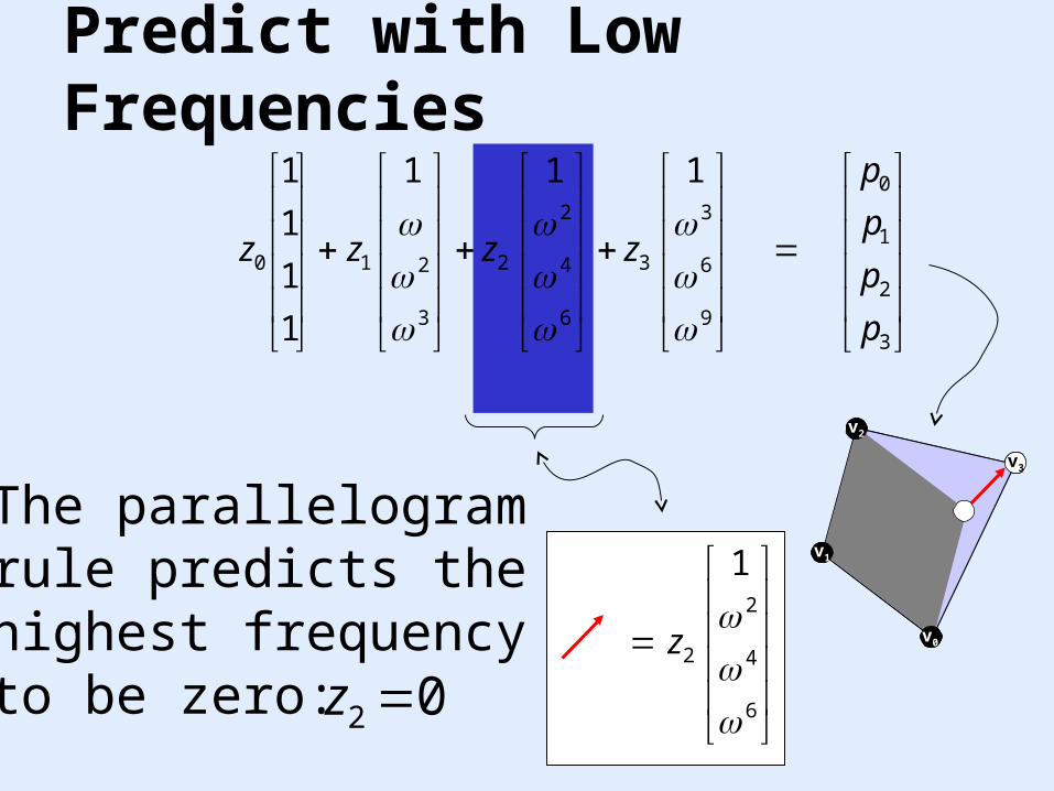
The parallelogramrule predicts thehighest frequencyto be zero: 02 z

Predict with Low Frequencies

3

2

1

0

9

6

3

3

6

4

2

2

3

210

111

1

1

1

1

p

p

p

p

zzzz

v2

v1

v0

v3v3

v2

v1

v0

v3v3

Overview

• Motivation

• Geometry Compression

• Frequency of Polygons

• Polygonal Prediction Rules

• Results

• DiscussionINFORMATIKINFORMATIK

Eliminate High Frequencies (1)

v3

v2

v1

v4

v0

v3v5

5

4

3

2

1

0

25

20

15

10

5

5

20

15

12

8

4

4

15

12

9

6

3

3

10

8

6

4

2

2

5

4

3

2

10

11111

1

1

1

1

1

1

p

p

p

p

p

p

zzzzzz

v3

v2

v1

v4

v0

v3v5

Eliminate High Frequencies (2)

v2

v3

v1

v0

v4

v1

v0

v4

v2

v3

4

3

2

1

0

15

12

8

4

4

12

9

6

3

3

8

6

4

2

2

4

3

210

1111

1

1

1

1

1

p

p

p

p

p

zzzzz

Eliminate High Frequencies (3)

4

3

2

1

0

15

12

8

4

4

12

9

6

3

3

8

6

4

2

2

4

3

210

1111

1

1

1

1

1

p

p

p

p

p

zzzzz

v1

v0

v4

v3

v2

v1

v0

v4

v3

v2

Computing the Coefficients

given k of n points are known:1. write polygon in Fourier basis2. put n-k highest frequencies to zero3. invert known sub-matrix4. calculate prediction coefficients

1

2

1

0

1

2

1

0

)1)(1()1(21

)1(242

12

1

1

1

1111

1

nnnnnn

n

n

p

p

p

p

z

z

z

z

n

knownpoints

missingpoints

Example: n = 5, k = 3

v0

v1

v4

v2

v3

4

3

2

1

0

4

3

2

1

0

151284

12963

8642

432

1

1

1

1

11111

5

1

p

p

p

p

p

z

z

z

z

z

4

1

0

4

1

0

154

4

1

1

111

5

1

p

p

p

z

z

z

4

1

0

444140

141110

040100

4

1

0

p

p

p

iii

iii

iii

z

z

z 4041010000 pipipiz

4141110101 pipipiz

4441410404 pipipiz

missingpoints

v0

v1

v4

v2

v3

knownpoints

Example: n = 5, k = 3

48

12

025

1zzzp

)()(5

1444141040

8414111010

2404101000 pipipipipipipipipi

444

814

204

141

811

201

040

810

200

5

)(

5

)(

5p

iiip

iiip

iii

0c 1c 4c

v0

v1

v4

v2

v3

missingpoints

4

3

2

1

0

4

3

2

1

0

151284

12963

8642

432

1

1

1

1

11111

5

1

p

p

p

p

p

z

z

z

z

z

knownpoints

Polygonal Predictors

v2v1

v0v3

v2v1

v0 v3

c0 = 1.0c1 = -1.6180c2 = 1.6180

c0 = 1.0c1 = -2.0c2 = 2.0

v2v1

v0 v3

c0 = 1.0c1 = -2.2470c2 = 2.2470

v2v1

v0v3

c0 = 1.0c1 = -2.4142c2 = 2.4142

• three vertices are known

v2v1

v0

v4

v3

c0 = 0.8090c1 = -0.3090c2 = -0.3090c3 = 0.8090

v3

v2

v0 v3

c0 = 1.0c1 = -1.0c2 = 1.0c3 = -1.0c4 = 1.0

v4v5

c0 = 0.9009c1 = -0.6234c2 = 0.2225c3 = 0.2225c4 = -0.6234c5 = 0.9009v2v1

v0 v3

v4

v5

v6

v2v1

v0 v3

v4

c0 = 1.0 c1 = -1.0 c2 = 1.0 c3 = -1.0 c4 = 1.0 c5 = -1.0 c6 = 1.0

v7

v5v6

v1

• one vertex is missing

Overview

• Motivation

• Geometry Compression

• Frequency of Polygons

• Polygonal Prediction Rules

• Results

• DiscussionINFORMATIKINFORMATIK

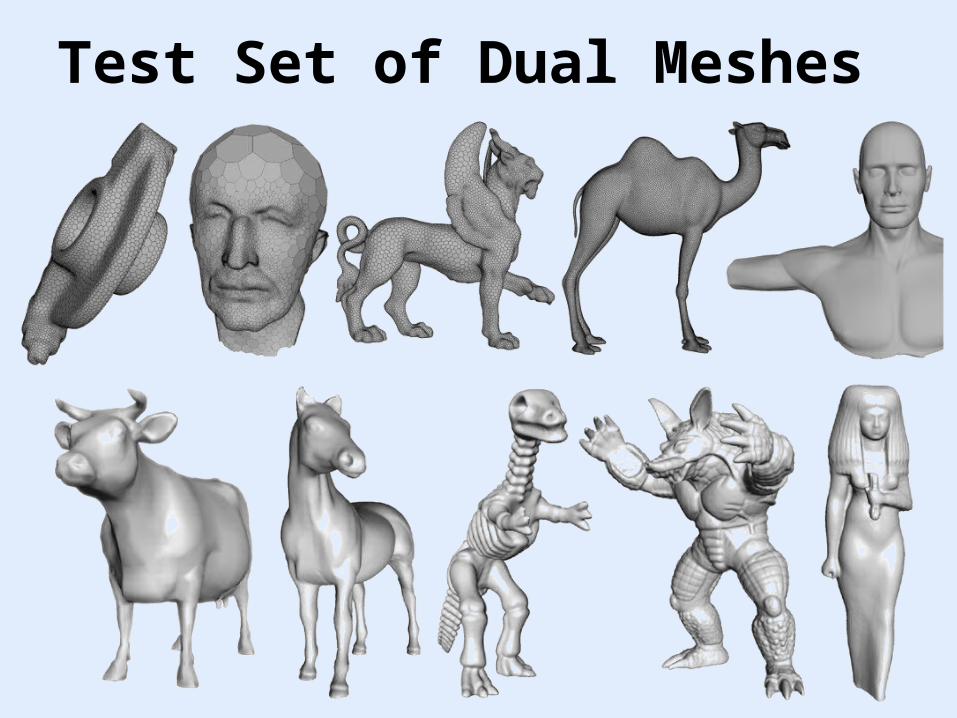
Test Set of Dual Meshes

Parallelogram vs. Polygonal

Prediction Rule Histogram

hexagon hexagon hexagon

heptagon heptagon heptagon

pentagon pentagon pentagon

octagon octagon octagon

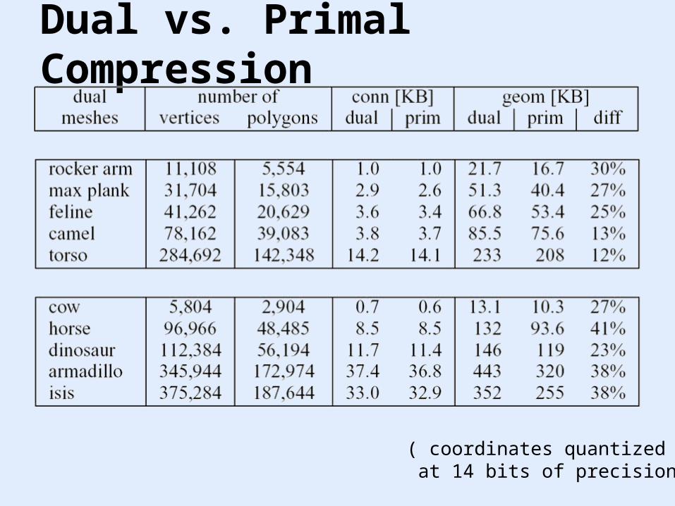
Dual vs. Primal Compression

( coordinates quantized at 14 bits of precision )

Average Prediction Error

Overview

• Motivation

• Geometry Compression

• Frequency of Polygons

• Polygonal Prediction Rules

• Results

• DiscussionINFORMATIKINFORMATIK

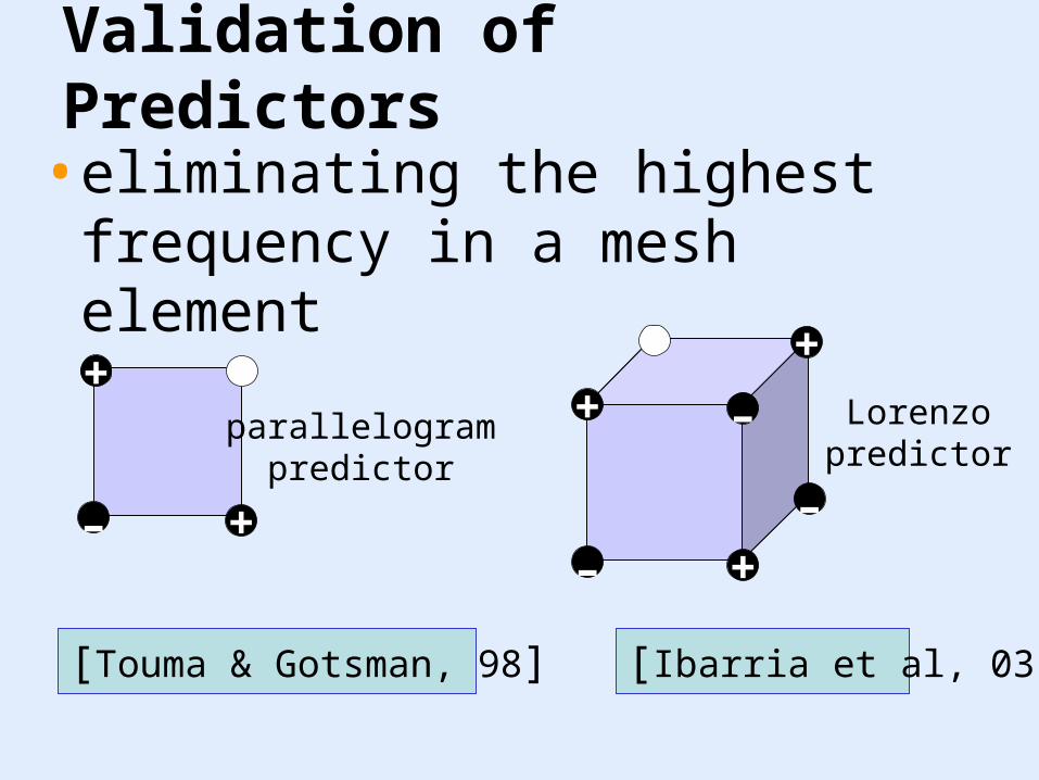
Validation of Predictors

• eliminating the highest frequency in a mesh element

– +

+parallelogram

predictor

[Touma & Gotsman, 98]

+

– +–

+ –

+Lorenzopredictor

[Ibarria et al, 03]

Exact barycentric prediction

• after dualization polygons of even order have a highest frequency of zero

Thank You

INFORMATIKINFORMATIK