TECHNICAL ADVANCE Matrix approach to land carbon cycle modeling: A case study with the Community Land Model Yuanyuan Huang 1,2 * | Xingjie Lu 1,3 * | Zheng Shi 1 | David Lawrence 4 | Charles D. Koven 5 | Jianyang Xia 6,7 | Zhenggang Du 7 | Erik Kluzek 4 | Yiqi Luo 1,3,8 1 Department of Microbiology and Plant Biology, University of Oklahoma, Norman, OK, USA 2 Now at Laboratoire des Sciences du Climat et de l’Environnement, Gif-sur-Yvette, France 3 Center for Ecosystem Science and Society, Northern Arizona University, Flagstaff, AZ, USA 4 Climate and Global Dynamics Division, National Center for Atmospheric Research, Boulder, CO, USA 5 Earth Sciences Division, Lawrence Berkeley National Laboratory, Berkeley, CA, USA 6 Tiantong National Forest Ecosystem Observation and Research Station, School of Ecological and Environmental Sciences, East China Normal University, Shanghai, China 7 Research Center for Global Change and Ecological Forecasting, East China Normal University, Shanghai, China 8 Department of Earth System Science, Tsinghua University, Beijing, China Correspondence Yuanyuan Huang, Laboratoire des Sciences du Climat et de l’Environnement, Gif-sur- Yvette, France. Email: [email protected] Xingjie Lu, Center for Ecosystem Science and Society, Northern Arizona University, Flagstaff, AZ, USA. Email: [email protected] Funding information US Department of Energy, Grant/Award Number: DE-SC0008270, DE-SC00114085; US National Science Foundation (NSF), Grant/Award Number: EF 1137293, OIA- 1301789 Abstract The terrestrial carbon (C) cycle has been commonly represented by a series of C balance equations to track C influxes into and effluxes out of individual pools in earth system models (ESMs). This representation matches our understanding of C cycle processes well but makes it difficult to track model behaviors. It is also com- putationally expensive, limiting the ability to conduct comprehensive parametric sen- sitivity analyses. To overcome these challenges, we have developed a matrix approach, which reorganizes the C balance equations in the original ESM into one matrix equation without changing any modeled C cycle processes and mechanisms. We applied the matrix approach to the Community Land Model (CLM4.5) with verti- cally-resolved biogeochemistry. The matrix equation exactly reproduces litter and soil organic carbon (SOC) dynamics of the standard CLM4.5 across different spatial- temporal scales. The matrix approach enables effective diagnosis of system proper- ties such as C residence time and attribution of global change impacts to relevant processes. We illustrated, for example, the impacts of CO 2 fertilization on litter and SOC dynamics can be easily decomposed into the relative contributions from C input, allocation of external C into different C pools, nitrogen regulation, altered soil environmental conditions, and vertical mixing along the soil profile. In addition, the matrix tool can accelerate model spin-up, permit thorough parametric sensitivity tests, enable pool-based data assimilation, and facilitate tracking and benchmarking of model behaviors. Overall, the matrix approach can make a broad range of future modeling activities more efficient and effective. KEYWORDS carbon storage, CO 2 fertilization, data assimilation, residence time, soil organic matter 1 | INTRODUCTION Terrestrial ecosystems absorb approximately 30% of the anthro- pogenic carbon dioxide (CO 2 ) emissions, which partially *Authors co-lead the research. Received: 13 August 2017 | Revised: 9 October 2017 | Accepted: 10 October 2017 DOI: 10.1111/gcb.13948 1394 | © 2017 John Wiley & Sons Ltd wileyonlinelibrary.com/journal/gcb Glob Change Biol. 2018;24:1394–1404.

Welcome message from author
This document is posted to help you gain knowledge. Please leave a comment to let me know what you think about it! Share it to your friends and learn new things together.
Transcript

T E C HN I C A L AD VAN C E
Matrix approach to land carbon cycle modeling: A case studywith the Community Land Model
Yuanyuan Huang1,2* | Xingjie Lu1,3* | Zheng Shi1 | David Lawrence4 |
Charles D. Koven5 | Jianyang Xia6,7 | Zhenggang Du7 | Erik Kluzek4 | Yiqi Luo1,3,8
1Department of Microbiology and Plant
Biology, University of Oklahoma, Norman,
OK, USA
2Now at Laboratoire des Sciences du Climat
et de l’Environnement, Gif-sur-Yvette,
France
3Center for Ecosystem Science and Society,
Northern Arizona University, Flagstaff, AZ,
USA
4Climate and Global Dynamics Division,
National Center for Atmospheric Research,
Boulder, CO, USA
5Earth Sciences Division, Lawrence
Berkeley National Laboratory, Berkeley, CA,
USA
6Tiantong National Forest Ecosystem
Observation and Research Station, School
of Ecological and Environmental Sciences,
East China Normal University, Shanghai,
China
7Research Center for Global Change and
Ecological Forecasting, East China Normal
University, Shanghai, China
8Department of Earth System Science,
Tsinghua University, Beijing, China
Correspondence
Yuanyuan Huang, Laboratoire des Sciences
du Climat et de l’Environnement, Gif-sur-
Yvette, France.
Email: [email protected]
Xingjie Lu, Center for Ecosystem Science
and Society, Northern Arizona University,
Flagstaff, AZ, USA.
Email: [email protected]
Funding information
US Department of Energy, Grant/Award
Number: DE-SC0008270, DE-SC00114085;
US National Science Foundation (NSF),
Grant/Award Number: EF 1137293, OIA-
1301789
Abstract
The terrestrial carbon (C) cycle has been commonly represented by a series of C
balance equations to track C influxes into and effluxes out of individual pools in
earth system models (ESMs). This representation matches our understanding of C
cycle processes well but makes it difficult to track model behaviors. It is also com-
putationally expensive, limiting the ability to conduct comprehensive parametric sen-
sitivity analyses. To overcome these challenges, we have developed a matrix
approach, which reorganizes the C balance equations in the original ESM into one
matrix equation without changing any modeled C cycle processes and mechanisms.
We applied the matrix approach to the Community Land Model (CLM4.5) with verti-
cally-resolved biogeochemistry. The matrix equation exactly reproduces litter and
soil organic carbon (SOC) dynamics of the standard CLM4.5 across different spatial-
temporal scales. The matrix approach enables effective diagnosis of system proper-
ties such as C residence time and attribution of global change impacts to relevant
processes. We illustrated, for example, the impacts of CO2 fertilization on litter and
SOC dynamics can be easily decomposed into the relative contributions from C
input, allocation of external C into different C pools, nitrogen regulation, altered soil
environmental conditions, and vertical mixing along the soil profile. In addition, the
matrix tool can accelerate model spin-up, permit thorough parametric sensitivity
tests, enable pool-based data assimilation, and facilitate tracking and benchmarking
of model behaviors. Overall, the matrix approach can make a broad range of future
modeling activities more efficient and effective.
K E YWORD S
carbon storage, CO2 fertilization, data assimilation, residence time, soil organic matter
1 | INTRODUCTION
Terrestrial ecosystems absorb approximately 30% of the anthro-
pogenic carbon dioxide (CO2) emissions, which partially*Authors co-lead the research.
Received: 13 August 2017 | Revised: 9 October 2017 | Accepted: 10 October 2017
DOI: 10.1111/gcb.13948
1394 | © 2017 John Wiley & Sons Ltd wileyonlinelibrary.com/journal/gcb Glob Change Biol. 2018;24:1394–1404.

counterbalances anthropogenic CO2 emission and, thus, plays an
important role in mitigating future climate warming (Canadell et al.,
2007). The scientific community relies strongly on global land carbon
(C) models to synthesize mechanisms that regulate land-atmosphere
CO2 exchanges, quantify responses of land CO2 fluxes to external
forcing, and predict future land C-uptake strength (Ciais et al., 2013).
For example, predictions of future CO2 dynamics in the 5th Intergov-
ernmental Panel on Climate Change (IPCC) report are primarily derived
from global models (with the land C model as a key component) partic-
ipated in the Coupled Model Intercomparison Project Phase 5
(CMIP5). Despite their importance in climate change assessment and
research, global land C models possess some inherent shortcomings,
such as low traceability due to their complexity, large computational
resources required for spin-up, and computational costs being too high
to conduct thorough sensitivity analysis (Friedlingstein et al., 2014; Lu,
Wang, Ziehn, & Dai, 2013; Luo et al., 2009; Washington, Buja, & Craig,
2009). It is imperative to develop innovative approaches to make glo-
bal models a more effective tool for C cycle research.
Global land C models typically represent hundreds of biophysical,
biogeochemical, and ecological processes interacting with each other
across different spatial-temporal timescales to mimic real world C
dynamics. C dynamics can be conceptually described by a series of C
balance equations, capturing C input through photosynthesis, transfers
among compartments, losses through respiration and land use or dis-
turbances. However, sophisticated behaviors arise when model struc-
tures (e.g., the number of C pools and explicitly represented processes)
differ, model parameters vary, and/or initial and boundary conditions
(e.g., temperature) evolve with system dynamics. Without a systematic
framework, it is difficult to disentangle contributions from a specific
component to the final model outputs, as each element can potentially
interact with other elements of the system. The soil organic matter
(SOM) decomposition rate, for example, is regulated by temporal and/
or spatial varying vegetation characteristics (e.g., litter quality and
rooting depth), soil thermal dynamics (e.g., soil temperature and
freeze-thaw cycle), hydrological conditions (e.g., soil moisture), edaphic
factors (e.g., soil texture), redox status, and nutrient levels (Luo et al.,
2016). SOM decomposition, on the other hand, can potentially feed
back to all of these processes through different mechanisms. In addi-
tion to being complex, global land C models are computationally
expensive. Land C models, mostly due to slow soil C processes, take
long time to stabilize. With a typical 1° 9 1° spatial resolution, it nor-
mally takes thousands of processor hours to spin-up a model to the
steady state (Washington et al., 2009), which is normally not afford-
able to most of the scientific community, and which becomes particu-
larly expensive when varying parameters, such that every parameter
perturbation must be equilibrated separately.
The complex nature of these global models and associated high
computational costs limit our understanding of model results. For
example, simulated land C fluxes in CMIP5 range from a source of
165 PgC to a sink of 758 PgC accumulated over 1,850–2,100
(Friedlingstein et al., 2014). Reasons for such a large discrepancy
among models are difficult to track and the credibility from modeling
are discounted. As they develop, land C models tend to incorporate
more and more processes, making them more complex. For instance,
microbial activities (Wieder et al., 2015), soil C vertical profiles (Koven
et al., 2013), plant species interactions (Fisher et al., 2015; Weng
et al., 2015), nutrient regulations (Gerber, Hedin, Oppenheimer,
Pacala, & Shevliakova, 2010; Thomas, Brookshire, & Gerber, 2015),
crop dynamics (Lu, Jin, & Kueppers, 2015) and disturbances (Landry,
Price, Ramankutty, Parrott, & Matthews, 2016; Shevliakova et al.,
2009; Yue et al., 2014) are all considered to be important components
that have been included in land models in recent years. As a result,
computational requirements surge further and become a bottleneck
for progress. It is almost impossible to get a full picture of the sensitiv-
ity of different C cycling processes to relevant parameters across the
globe. To conduct sensitivity tests, compromises have to be made, for
example, by choosing a small set instead of all relevant parameters,
prescribing initial conditions instead of through spin-up, or focusing on
a small local range instead of the global sensitivity.
There is a need for innovative tools to systematically tackle the
efficiency and traceability challenges faced by land C models. Several
model intercomparison projects (MIPs), such as CMIP5, TRENDY
(http://dgvm.ceh.ac.uk/node/9) and MsTMIP (Huntzinger et al.,
2013), were designed to diagnose, interpret and address disagree-
ments in model performance and to track uncertainties in future C
projections. These MIPs are helpful in identifying mismatches and
uncertainties among models, but remain largely descriptive rather than
insightful in tracing the origins of model differences. Xia, Luo, Wang,
and Hararuk (2013) developed a new framework to decompose the
complex model outputs into traceable components and track modeled
ecosystem C storage capacity through ecosystem C input (e.g., net pri-
mary productivity, NPP), and residence time. Unfortunately, this
framework is only applicable to steady state conditions. Koven, Lawr-
ence, and Riley (2015) used a similar approach to decompose the
dynamics of several CMIP5 model responses to CO2, climate, and both
CO2 and climate together using a 2-pool (live and dead) approximation
and concluded that model dynamics of both pools to all sets of forc-
ings are largely driven by productivity rather than turnover, which
likely represents a consistent bias shared by models. Luo et al. (2017)
explored transient dynamics of modeled terrestrial C in a 3-dimen-
sional (D) parameter space, i.e., C input, residence time, and the stor-
age potential which reflects the difference between C storage capacity
and actual C storage. The 3-D parameter space provides a novel theo-
retical framework to evaluate and trace transient C dynamics. It can
also potentially be used to understand and fundamentally improve the
low traceability issue of land models. The transient dynamics analysis
proposed by Luo et al. (2017) is based on matrix representation of C
cycle, which has not yet been realized in global models.
To address the above limitations, we develop a matrix approach
to global land C modeling. Specifically, we reorganize the 70 carbon
balance equations in the Community Land Model Version 4.5
(CLM4.5) into one matrix equation to describe C transfer among
organic pools in 10 soil layers. We first verify that the matrix equa-
tion fully reproduces simulation results of the original CLM4.5. Then,
we demonstrate scientific and technical advantages of this matrix
approach in two aspects: the calculation of diagnostic parameters,
HUANG ET AL. | 1395
and the attribution of the global C cycle response to CO2 increases
to various component processes. We also discuss additional novel
applications of the matrix approach for model spin-up, traceability
analysis, data assimilation, and benchmark analysis.
2 | MATERIALS AND METHODS
2.1 | CLM4.5 overview
Community Land Model Version 4.5 couples processes that regulate
terrestrial energy, water, C and other biogeochemical cycles (Koven
et al., 2013; Oleson et al., 2013). Specifically for biogeochemistry,
CLM4.5 tracks vertically-resolved C and nitrogen (N) state variables in
different vegetation, litter and SOM pools. We focus mainly on
CLM4.5bgc which adopts the Century style soil C pool structure
(Koven et al., 2013).
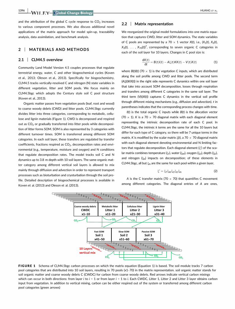
Organic matter passes from vegetation pools (leaf, root and wood)
to coarse woody debris (CWD) and litter pools. CLM4.5bgc currently
divides litter into three categories, corresponding to metabolic, cellu-
lose and lignin materials (Figure 1). CWD is decomposed and respired
out as CO2 or gradually transferred into litter pools while decomposi-
tion of litter forms SOM. SOM is also represented by 3 categories with
different turnover times. SOM is transferred among different SOM
categories. In each soil layer, these transfers are regulated by transfer
coefficients, fractions respired as CO2, decomposition rates and envi-
ronmental (e.g., temperature, moisture and oxygen) and N conditions
that regulate decomposition rates. The model tracks soil C and N
dynamics up to 3.8 m depth with 10 soil layers. The same organic mat-
ter category among different vertical soil layers is allowed to mix
mainly through diffusion and advection in order to represent transport
processes such as bioturbation and cryoturbation through the soil pro-
file. Detailed description of biogeochemical processes is available in
Koven et al. (2013) and Oleson et al. (2013).
2.2 | Matrix representation
We reorganized the original model formulations into one matrix equa-
tion that captures CWD, litter and SOM dynamics. The state variables
of C pools are represented by a 70 9 1 vector X(t), i.e., (X1(t), X2(t),
X3(t), . . . , X70(t))T, corresponding to seven organic C categories in
each of the soil layer for 10 layers. Changes in C pool size is:
dXðtÞdt
¼ BðtÞIðtÞ � AnðtÞKXðtÞ � VðtÞXðtÞ (1)
where B(t)I(t) (70 9 1) is the vegetation C inputs, which are distributed
along the soil profile among CWD and litter pools. The second term
(Aξ(t)KX(t)) in the right side represents C dynamics within one soil layer
that take into account SOM decomposition, losses through respiration
and transfers among different C categories in the same soil layer. The
third term (V(t)X(t)) captures C dynamics in the vertical soil profile
through different mixing mechanisms (e.g., diffusion and advection). t in
parentheses indicates that the corresponding process changes with time.
I(t) is the total organic C inputs while B(t) is the allocation vector
(70 9 1). K is a 70 9 70 diagonal matrix with each diagonal element
representing the intrinsic decomposition rate of each C pool. In
CLM4.5bgc, the intrinsic k terms are the same for all the 10 layers but
differ for each type of C category, so there will be 7 unique terms in the
matrix. K is modified by the scalar matrix ξ(t), a 70 9 70 diagonal matrix
with each diagonal element denoting environmental and N limiting fac-
tors that regulate decomposition. Each diagonal element (ξ0) of the sca-
lar matrix combines temperature (ξT), water (ξW), oxygen (ξO), depth (ξD),
and nitrogen (ξN) impacts on decomposition; of these elements in
CLM4.5bgc, all but ξN are the same for each pool within a given layer,
n0 ¼ nTnWnOnDnN (2)
A is the C transfer matrix (70 9 70) that quantifies C movement
among different categories. The diagonal entries of A are ones,
Coarse woody debrisCWDCx1–10
Fast SOMSoil 1
x41–50
Metabolic litterLitter 1x11–20
Lignin litterLitter 3x31–40
Cellulose litter Litter 2x21–30
Slow SOMSoil 2
x51–60
Passive SOMSoil 3
x61–70
CO2CO2 CO2 CO2
CO2CO2 CO2
10 Layersvertical mix
F IGURE 1 Schema of CLM4.5bgc carbon processes on which the matrix equation (Equation 1) is based. The soil module tracks 7 carbonpool categories that are distributed into 10 soil layers, resulting in 70 pools (x1–70) in the matrix representation. soil organic matter stands forsoil organic matter and coarse woody debris C (CWDC) for carbon from coarse woody debris. Red arrows indicate vertical carbon mixingswhich can occur in both directions: from layer i to i + 1 or from layer i + 1 to i. Each CWDC, Litter 1, Litter 2 and Litter 3 layer obtains carboninput from vegetation. In addition to vertical mixing, carbon can be either respired out of the system or transferred among different carbonpool categories (green arrows)
1396 | HUANG ET AL.
corresponding to the entire decomposition fluxes produced from
each C pool. The non-diagonal entries (aij) represent the fraction
of C moving from the jth to the ith pool. For example, a42 indi-
cates the fraction of C from the 2nd pool that is transferred to
the 4th pool during decomposition. In this way, the ith row of
the A matrix summarizes the fraction that exits and enters the ith
pool. In CLM4.5bgc, transfer coefficients are set to be the same
in each soil layer. The structure of A is illustrated through the
block matrix,
A ¼
A11 0 0 0 0 0 00 A22 0 0 0 0 0
A31 0 A33 0 0 0 0A41 0 0 A44 0 0 00 A52 A53 0 A55 A56 A570 0 0 A64 A65 A66 00 0 0 0 A75 A76 A77
0BBBBBBBB@
1CCCCCCCCA
(3)
Each block entry represents a 10 9 10 matrix corresponding to
10 soil layers. The diagonal block entries (A11, A22, A33, A44, A55,
A66, A77) denote seven 10 9 10 identical matrices, while the non-
diagonal block entries (non-zeros) are 10 9 10 diagonal matrices
with different transfer coefficients for different matrices. Numbers
correspond to seven C categories, i.e., CWD, litter1, litter2, litter3,
soil1, soil2 and soil3. For example, A31 indicates the fraction of C
transferred from CWD to litter2. Since the transfer coefficient (f31)
is the same for different soil layers,
A31¼diagð�f31;�f31;�f31;�f31;�f31;�f31;�f31;�f31;�f31;�f31Þ (4)
V(t) denotes the vertical C mixing coefficient matrix,
VðtÞ ¼
V11 0 0 0 0 0 00 V22ðtÞ 0 0 0 0 00 0 V33ðtÞ 0 0 0 00 0 0 V44ðtÞ 0 0 00 0 0 0 V55ðtÞ 0 00 0 0 0 0 V66ðtÞ 00 0 0 0 0 0 V77ðtÞ
0BBBBBBBB@
1CCCCCCCCA
(5)
Each of the diagonal block is a tridiagonal matrix (except V11)
that describes mixings of the corresponding C pool category among
different soil layers. CLM4.5bgc assumes no vertical mixings of
CWD. Therefore, V11 is a zero matrix. As the vertical mixing rates
are not differentiated among different C pool categories, V22, V33,
V44, V55, V66, and V77 are identical with the following structure,
V22 ¼ diagðz1; z2; . . .; z10Þ�1
g1 �g1 0 0 � � � 0 0 0
�h2 h2 þ g2 �g2 0 � � � 0 0 0
0 �h3 h3 þ g3 �g3 � � � 0 0 0
0 0 �h4 h4 þ g4 � � � 0 0 0
..
. ... ..
. ... . .
. ... ..
. ...
0 0 0 0 � � � h8 þ g8 �g8 0
0 0 0 0 � � � �h9 h9 þ g9 �g90 0 0 0 � � � 0 �h10 h10
0BBBBBBBBBBBBBB@
1CCCCCCCCCCCCCCA
(6)
where the subscript numbers denote soil layers; g and h are vertical
mixing rates (in unit of depth/time, e.g., m/year) of C between the
current soil layer and the upper layer and between the current and
the lower layer respectively. z indicates the depth of each soil layer.
In CLM4.5bgc, gi = hi+1, i = 1, . . ., 9.
2.3 | Test and applications of matrix representationof CLM4.5bgc
We incorporated this matrix representation into CLM4.5bgc and ran
in parallel with the original model (hereafter, the default) with the
same initial conditions and forcing. To verify the matrix representa-
tion, we conducted two tests: (i) a 1,000-year simulation at a single
site (Brazil, 7°S, 55°W) starting from near-zero carbon stocks; and
(ii), a transient 10-year global simulation starting from spun-up 1,850
initial conditions.
According to the mathematical foundation for transient C
dynamics derived in Luo et al. (2017), the behavior of most land C
cycle models can be diagnosed by three parameters: C input, resi-
dence time, and storage potential. To calculate these parameters,
Equation 1 can be rewritten as,
XðtÞ ¼ ðAnðtÞK þ VðtÞÞ�1BðtÞIðtÞ � ðAnðtÞK þ VðtÞÞ�1 dXðtÞdt
(7)
where ðAnðtÞK þ VðtÞÞ�1BðtÞIðtÞ is the C storage capacity, which
quantifies the maximum amount of C a system can store at the
given instantaneous environmental condition at time t. C storage
capacity consists of two components: C input IðtÞ and residence time
ðAnðtÞK þ VðtÞÞ�1BðtÞ under given C input and environmental condi-
tions. And ðAnðtÞK þ VðtÞÞ�1 dXðtÞdt is the C storage potential, i.e., the
difference between the storage capacity and the actual C storage.
To obtain ecosystem-level C residence time, we extended these
70 C pools to include three vegetation pools: leaf, stem and root.
We lumped the leaf transfer pool and storage pool from the original
model into one leaf pool. Similarly, live and dead stem transfer pools
and storage pools were treated as one stem pool, and live and dead
coarse root transfer pools and storage pools, fine root transfer pool
and storage pool make the root pool in the matrix representation.
We ran the matrix module embedded in a global version of
CLM4.5bgc and calculated the matrix diagnostics at an annual
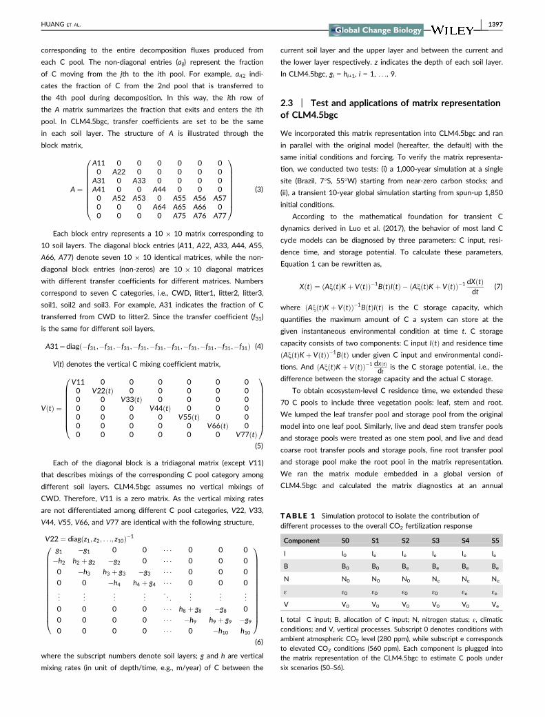
TABLE 1 Simulation protocol to isolate the contribution ofdifferent processes to the overall CO2 fertilization response
Component S0 S1 S2 S3 S4 S5
I I0 Ie Ie Ie Ie Ie
B B0 B0 Be Be Be Be
N N0 N0 N0 Ne Ne Ne
ɛ ɛ0 ɛ0 ɛ0 ɛ0 ɛe ɛe
V V0 V0 V0 V0 V0 Ve
I, total C input; B, allocation of C input; N, nitrogen status; ɛ, climatic
conditions; and V, vertical processes. Subscript 0 denotes conditions with
ambient atmospheric CO2 level (280 ppm), while subscript e corresponds
to elevated CO2 conditions (560 ppm). Each component is plugged into
the matrix representation of the CLM4.5bgc to estimate C pools under
six scenarios (S0–S6).
HUANG ET AL. | 1397

timestep with temporal averaged matrix elements. To verify matrix
diagnostics, we compared C storage capacity after 360-year matrix
simulation with the steady state ecosystem C storage (DC < 0.001%
of total ecosystem C) obtained from CLM4.5bgc default accelerated
spin-up. We also examined a permafrost site in Alaska (63°530N,
149°130W) to illustrate the difference between calculation of resi-
dence time from the matrix approach and the standard method by
dividing carbon stocks by fluxes.
With the matrix approach, it is easy to disentangle different
processes that regulate C dynamics. To illustrate such functional-
ity, we examined the responses of dead C (CWD, litter and SOM)
to CO2 fertilization. We identified that changes in total C input,
allocation to different C pools, N status, environmental conditions
and vertical mixing are potential processes contributing to the
overall CO2 fertilization effects. We first ran the default
CLM4.5bgc with 280 ppm atmospheric CO2 concentration for
1:1 line
(a) (b)
(c) (d)
(e) (f)
F IGURE 2 Comparisons of dead C pools simulated from the matrix equation (Equation 1) vs. default CLM4.5bgc simulation at a Brazil site(7oS, 55oW). The matrix module was run in parallel with the default CLM4.5bgc from scratch for 1,000 years. Left panels display coarse woodydebris C (CWDC, a), total litter C (c) and total soil C (e) from the matrix simulation, and the right panels (b, d, f) plot corresponding simulationresults from the default (x axes) vs. from the matrix module (y axes). The 1:1 lines indicate simulated C pools from the matrix module 100%match these from the default CLM4.5bgc model
1398 | HUANG ET AL.
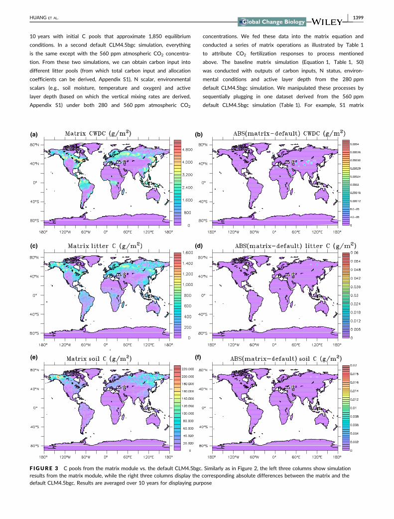
10 years with initial C pools that approximate 1,850 equilibrium
conditions. In a second default CLM4.5bgc simulation, everything
is the same except with the 560 ppm atmospheric CO2 concentra-
tion. From these two simulations, we can obtain carbon input into
different litter pools (from which total carbon input and allocation
coefficients can be derived, Appendix S1), N scalar, environmental
scalars (e.g., soil moisture, temperature and oxygen) and active
layer depth (based on which the vertical mixing rates are derived,
Appendix S1) under both 280 and 560 ppm atmospheric CO2
concentrations. We fed these data into the matrix equation and
conducted a series of matrix operations as illustrated by Table 1
to attribute CO2 fertilization responses to process mentioned
above. The baseline matrix simulation (Equation 1, Table 1, S0)
was conducted with outputs of carbon inputs, N status, environ-
mental conditions and active layer depth from the 280 ppm
default CLM4.5bgc simulation. We manipulated these processes by
sequentially plugging in one dataset derived from the 560 ppm
default CLM4.5bgc simulation (Table 1). For example, S1 matrix
(a) (b)
(c) (d)
(e) (f)
F IGURE 3 C pools from the matrix module vs. the default CLM4.5bgc. Similarly as in Figure 2, the left three columns show simulationresults from the matrix module, while the right three columns display the corresponding absolute differences between the matrix and thedefault CLM4.5bgc. Results are averaged over 10 years for displaying purpose
HUANG ET AL. | 1399

simulation was conducted with total C input from CLM4.5bgc
560 ppm and all other conditions from CLM4.5bgc 280 ppm; S2
matrix simulation was conducted with total C input and the allo-
cation from CLM4.5bgc 560 ppm while the remaining conditions
based on CLM4.5bgc 280 ppm, and so on. Therefore, the contri-
bution of total C input is derived from the difference between S1
and S0, and the contribution of the allocation is the difference
between S2 and S1 and so on.
3 | RESULTS AND DISCUSSION
3.1 | Verification of matrix representation
The matrix model perfectly reproduces the default patterns in both
long timescale single site (Figure 2) and shorter timescale global
(Figure 3) simulations. At the Brazil site, C stocks accumulate with
time since the run was initialized with small C stocks (Figure 2).
The matrix simulation follows exactly the same pattern as the
default, illustrated by the fact that points fall exactly on the 1:1
line (Figure 2). At the global scale, differences between the matrix
approach and the default CLM4.5bgc simulated C pools are essen-
tially zero (Figure 3). Simulated soil C can reach the level of
100,000 gC/m2 in the northern high latitudes, while the largest dif-
ference between the matrix and the default is only around
0.02 gC/m2.
3.2 | Application 1: 3D parameter space fordiagnosis of the original model
Tropical regions have more C input (Figure 4a) while northern high
latitudes are characterized by long C residence time (Figure 4b), both
of which characteristics can lead to high C storage capacity (Fig-
ure 4c). After 360-years matrix simulation, the difference between
diagnosed C storage capacity and the steady state C stock from a
full default CLM4.5bgc spin-up is small, with a difference around
0.5% in global C stock estimation. The small difference is valid for
most of the global grid cells despite regional variations (Figure 4d).
Starting from the near-zero initial condition, ecosystem C input,
residence time, storage capacity and the actual C storage increase
with time (Figure 5). The actual C storage chases C storage capacity
until both reach the system steady state. When the actual C storage
grows slower than C storage capacity, C storage potential increases
with time and vice versa. And C storage potential stays at 0 when
the system stabilizes. The rate of change in C storage is proportional
to C storage potential based on the mathematical properties derived
from Luo et al. (2017), and C storage potential offers an additional
diagnostic on transient C dynamics.
In addition to the 3rd dimension (C storage potential) that brings
novel angle in diagnosing global land C dynamics, the matrix also
expands our understanding on C residence time. The common prac-
tice of dividing total C stocks by fluxes offers an easy mathematical
(a) (b)
(c) (d)
F IGURE 4 (a) Ecosystem C input (i.e., net primary production, NPP), (b) ecosystem C residence time (transit time), and (c) ecosystem Cstorage capacity diagnosed from the matrix equation. (d) Difference between C storage capacity after 360 years of matrix simulation and thesteady state total carbon (DC < 0.001% of total global ecosystem C) from default CLM4.5 spin-up. Model configuration is slightly differentfrom simulations for Figure 3 with the decomp_depth_efolding (regulates the distribution of C input along the vertical profile) equals 10.0instead of 0.5 in addition to the initial condition. This set-up requires less time for the default CLM4.5 to reach the steady state criterion andreduces the chances that some grid cells (especially in the northern high latitudes) are not stabilized despite the global total carbon stock staysrelative stable
1400 | HUANG ET AL.
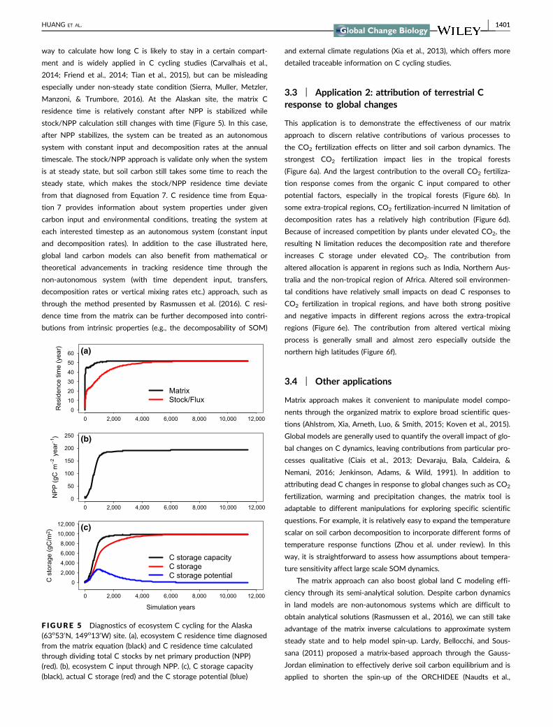
way to calculate how long C is likely to stay in a certain compart-
ment and is widely applied in C cycling studies (Carvalhais et al.,
2014; Friend et al., 2014; Tian et al., 2015), but can be misleading
especially under non-steady state condition (Sierra, Muller, Metzler,
Manzoni, & Trumbore, 2016). At the Alaskan site, the matrix C
residence time is relatively constant after NPP is stabilized while
stock/NPP calculation still changes with time (Figure 5). In this case,
after NPP stabilizes, the system can be treated as an autonomous
system with constant input and decomposition rates at the annual
timescale. The stock/NPP approach is validate only when the system
is at steady state, but soil carbon still takes some time to reach the
steady state, which makes the stock/NPP residence time deviate
from that diagnosed from Equation 7. C residence time from Equa-
tion 7 provides information about system properties under given
carbon input and environmental conditions, treating the system at
each interested timestep as an autonomous system (constant input
and decomposition rates). In addition to the case illustrated here,
global land carbon models can also benefit from mathematical or
theoretical advancements in tracking residence time through the
non-autonomous system (with time dependent input, transfers,
decomposition rates or vertical mixing rates etc.) approach, such as
through the method presented by Rasmussen et al. (2016). C resi-
dence time from the matrix can be further decomposed into contri-
butions from intrinsic properties (e.g., the decomposability of SOM)
and external climate regulations (Xia et al., 2013), which offers more
detailed traceable information on C cycling studies.
3.3 | Application 2: attribution of terrestrial Cresponse to global changes
This application is to demonstrate the effectiveness of our matrix
approach to discern relative contributions of various processes to
the CO2 fertilization effects on litter and soil carbon dynamics. The
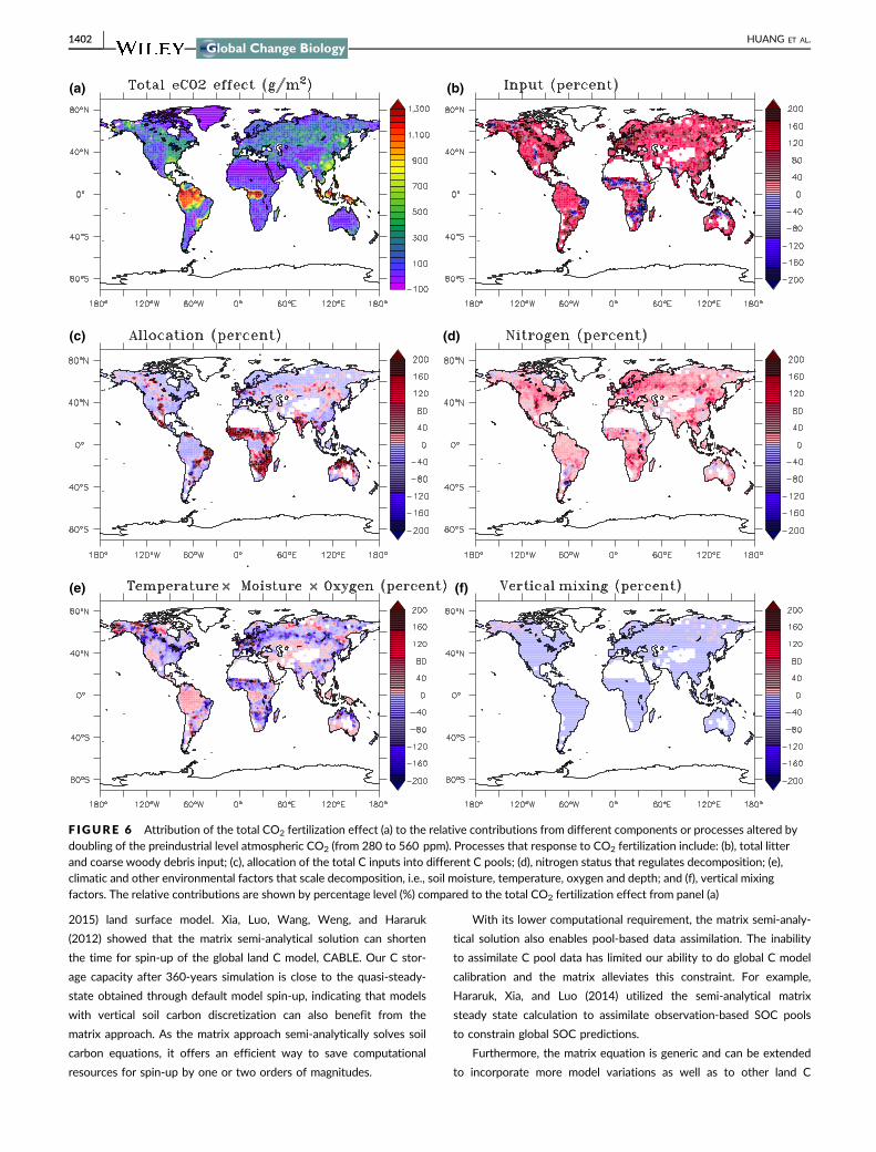
strongest CO2 fertilization impact lies in the tropical forests
(Figure 6a). And the largest contribution to the overall CO2 fertiliza-
tion response comes from the organic C input compared to other
potential factors, especially in the tropical forests (Figure 6b). In
some extra-tropical regions, CO2 fertilization-incurred N limitation of
decomposition rates has a relatively high contribution (Figure 6d).
Because of increased competition by plants under elevated CO2, the
resulting N limitation reduces the decomposition rate and therefore
increases C storage under elevated CO2. The contribution from
altered allocation is apparent in regions such as India, Northern Aus-
tralia and the non-tropical region of Africa. Altered soil environmen-
tal conditions have relatively small impacts on dead C responses to
CO2 fertilization in tropical regions, and have both strong positive
and negative impacts in different regions across the extra-tropical
regions (Figure 6e). The contribution from altered vertical mixing
process is generally small and almost zero especially outside the
northern high latitudes (Figure 6f).
3.4 | Other applications
Matrix approach makes it convenient to manipulate model compo-
nents through the organized matrix to explore broad scientific ques-
tions (Ahlstrom, Xia, Arneth, Luo, & Smith, 2015; Koven et al., 2015).
Global models are generally used to quantify the overall impact of glo-
bal changes on C dynamics, leaving contributions from particular pro-
cesses qualitative (Ciais et al., 2013; Devaraju, Bala, Caldeira, &
Nemani, 2016; Jenkinson, Adams, & Wild, 1991). In addition to
attributing dead C changes in response to global changes such as CO2
fertilization, warming and precipitation changes, the matrix tool is
adaptable to different manipulations for exploring specific scientific
questions. For example, it is relatively easy to expand the temperature
scalar on soil carbon decomposition to incorporate different forms of
temperature response functions (Zhou et al. under review). In this
way, it is straightforward to assess how assumptions about tempera-
ture sensitivity affect large scale SOM dynamics.
The matrix approach can also boost global land C modeling effi-
ciency through its semi-analytical solution. Despite carbon dynamics
in land models are non-autonomous systems which are difficult to
obtain analytical solutions (Rasmussen et al., 2016), we can still take
advantage of the matrix inverse calculations to approximate system
steady state and to help model spin-up. Lardy, Bellocchi, and Sous-
sana (2011) proposed a matrix-based approach through the Gauss-
Jordan elimination to effectively derive soil carbon equilibrium and is
applied to shorten the spin-up of the ORCHIDEE (Naudts et al.,
0102030405060
0 2,000 4,000 6,000 8,000 10,000 12,000
Res
iden
ce ti
me
(yea
r) (a)
MatrixStock/Flux
0
50
100
150
200
250
0 2,000 4,000 6,000 8,000 10,000 12,000
NPP
(gC
m−2
year
−1) (b)
0
2,000
4,000
6,000
8,000
10,000
12,000
0 2,000 4,000 6,000 8,000 10,000 12,000
C s
tora
ge (g
C/m
2 )
Simulation years
(c)
C storage capacityC storageC storage potential
F IGURE 5 Diagnostics of ecosystem C cycling for the Alaska(63o530N, 149o130W) site. (a), ecosystem C residence time diagnosedfrom the matrix equation (black) and C residence time calculatedthrough dividing total C stocks by net primary production (NPP)(red). (b), ecosystem C input through NPP. (c), C storage capacity(black), actual C storage (red) and the C storage potential (blue)
HUANG ET AL. | 1401
2015) land surface model. Xia, Luo, Wang, Weng, and Hararuk
(2012) showed that the matrix semi-analytical solution can shorten
the time for spin-up of the global land C model, CABLE. Our C stor-
age capacity after 360-years simulation is close to the quasi-steady-
state obtained through default model spin-up, indicating that models
with vertical soil carbon discretization can also benefit from the
matrix approach. As the matrix approach semi-analytically solves soil
carbon equations, it offers an efficient way to save computational
resources for spin-up by one or two orders of magnitudes.
With its lower computational requirement, the matrix semi-analy-
tical solution also enables pool-based data assimilation. The inability
to assimilate C pool data has limited our ability to do global C model
calibration and the matrix alleviates this constraint. For example,
Hararuk, Xia, and Luo (2014) utilized the semi-analytical matrix
steady state calculation to assimilate observation-based SOC pools
to constrain global SOC predictions.
Furthermore, the matrix equation is generic and can be extended
to incorporate more model variations as well as to other land C
× ×
,
,
(a) (b)
(e) (f)
(c) (d)
F IGURE 6 Attribution of the total CO2 fertilization effect (a) to the relative contributions from different components or processes altered bydoubling of the preindustrial level atmospheric CO2 (from 280 to 560 ppm). Processes that response to CO2 fertilization include: (b), total litterand coarse woody debris input; (c), allocation of the total C inputs into different C pools; (d), nitrogen status that regulates decomposition; (e),climatic and other environmental factors that scale decomposition, i.e., soil moisture, temperature, oxygen and depth; and (f), vertical mixingfactors. The relative contributions are shown by percentage level (%) compared to the total CO2 fertilization effect from panel (a)
1402 | HUANG ET AL.
models with different structures (Luo & Weng, 2011; Luo et al.,
2001, 2017; Sierra & Muller, 2015). The matrix equation offers a
general mathematic framework, which replicates the majority of cur-
rent SOM models and allows structural flexibility that facilitates
development of particular models at various levels of detail (Sierra &
Muller, 2015). We showed here that the matrix approach can repli-
cate the original land C model results even with vertically discretized
soil layers. The matrix is similarly flexible in accommodating more
variations, such as microbial dynamics and ecological demography
modeling, simply by adding additional elements in each matrix.
Divergences in modeled C pool structure are reflected in how many
dimensions the matrix has and interactions among matrix elements.
With its simplicity in coding, diagnostic capability, generic struc-
ture and computational efficiency, the matrix approach can improve
the efficiency of model intercomparison, benchmarking and uncer-
tainty assessment with an ensemble of matrix equations representing
the range of global land C model structures. In addition to CLM4.5
presented here, other global land models, such as CABLE (Xia et al.,
2012, 2013), LPJ-GUESS (Ahlstrom et al., 2015), CLM-CASA’(Har-
aruk et al., 2014) and CLM4.0 (Rafique et al., 2017; Wieder, Boehn-
ert, & Bonan, 2014), have showed that the matrix approach helped
model-data integration, model evaluation and improvement. And
matrix equations are also derived for the newly developed ORCHI-
DEE-MICT model (Guimberteau et al., 2017) which targets especially
on the high latitude regions. Collectively, the matrix reorganizations
of original models with a suite of novel matrix-based theory and
tools (Luo et al., 2017; Metzler & Sierra, 2017; Rasmussen et al.,
2016; Sierra et al., 2016; Xia et al., 2012, 2013) create a trackable
avenue for global model-data integration, benchmark and uncertainty
analyses. In addition, the matrix simulation can be conducted in
one’s personal computer (see Appendix S1 for an example MATLAB
program that can be run at the global scale), which creates a great
opportunity to explore carbon dynamics of earth system models (at
least offline) especially for educators and students.
ACKNOWLEDGEMENTS
This work was financially supported by US Department of Energy
grants DE-SC0008270, DE-SC00114085, and US National Science
Foundation (NSF) grants EF 1137293 and OIA-1301789.
ORCID
Yuanyuan Huang http://orcid.org/0000-0003-4202-8071
REFERENCES
Ahlstrom, A., Xia, J. Y., Arneth, A., Luo, Y. Q., & Smith, B. (2015). Impor-
tance of vegetation dynamics for future terrestrial carbon cycling.
Environmental Research Letters, 10, 054019. https://doi.org/10.1088/
1748-9326/10/5/054019
Canadell, J. G., Le Qu�er�e, C., Raupach, M. R., Field, C. B., Buitenhuis, E.
T., Ciais, P., . . . Marland, G. (2007). Contributions to accelerating
atmospheric CO2 growth from economic activity, carbon intensity,
and efficiency of natural sinks. Proceedings of the National Academy of
Sciences, 104, 18866–18870. https://doi.org/10.1073/pnas.
0702737104
Carvalhais, N., Forkel, M., Khomik, M., Bellarby, J., Jung, M., Migliavacca,
M., . . . Reichstein, M. (2014). Global covariation of carbon turnover
times with climate in terrestrial ecosystems. Nature, 514, 213–217.
https://doi.org/10.1038/nature13731
Ciais, P., Sabine, C., Bala, G., Bopp, L., Brovkin, V., Canadell, J., . . . Thornton,
P. (2013). Carbon and other biogeochemical cycles. In T. F. Stocker, D.
Qin, G.-K. Plattner, M. Tignor, S. K. Allen, J. Boschung, A. Nauels, Y.
Xia, V. Bex & P. M. Midgley (Eds.), Climate change 2013: The physical
science basis. Contribution of working group I to the fifth assessment
report of the intergovernmental panel on climate change (pp. 465–570).
Cambridge, UK and New York, NY: Cambridge University Press.
Devaraju, N., Bala, G., Caldeira, K., & Nemani, R. (2016). A model based
investigation of the relative importance of CO2-fertilization, climate
warming, nitrogen deposition and land use change on the global ter-
restrial carbon uptake in the historical period. Climate Dynamics, 47,
173–190. https://doi.org/10.1007/s00382-015-2830-8
Fisher, R. A., Muszala, S., Verteinstein, M., Lawrence, P., Xu, C., McDow-
ell, N. G., . . . Bonan, G. (2015). Taking off the training wheels: The
properties of a dynamic vegetation model without climate envelopes,
CLM4.5(ED). Geoscientific Model Development, 8, 3593–3619.
https://doi.org/10.5194/gmd-8-3593-2015
Friedlingstein, P., Meinshausen, M., Arora, V. K., Jones, C. D., Anav, A.,
Liddicoat, S. K., & Knutti, R. (2014). Uncertainties in CMIP5 climate
projections due to carbon cycle feedbacks. Journal of Climate, 27,
511–526. https://doi.org/10.1175/JCLI-D-12-00579.1
Friend, A. D., Lucht, W., Rademacher, T. T., Keribin, R., Betts, R., Cadule,
P., . . . Woodward, F. I. (2014). Carbon residence time dominates
uncertainty in terrestrial vegetation responses to future climate and
atmospheric CO2. Proceedings of the National Academy of Sciences of
the United States of America, 111, 3280–3285. https://doi.org/10.
1073/pnas.1222477110
Gerber, S., Hedin, L. O., Oppenheimer, M., Pacala, S. W., & Shevliakova,
E. (2010). Nitrogen cycling and feedbacks in a global dynamic land
model. Global Biogeochemical Cycles, 24, GB1001.
Guimberteau, M., Zhu, D., Maignan, F., Huang, Y., Yue, C., Dantec-
N�ed�elec, S., . . . Ciais, P. (2017). ORCHIDEE-MICT (revision 4126), a
land surface model for the high-latitudes: Model description and vali-
dation. Geoscientific Model Development Discussions, 10, 1–65.
https://doi.org/10.5194/gmd-2017-122
Hararuk, O., Xia, J. Y., & Luo, Y. Q. (2014). Evaluation and improvement
of a global land model against soil carbon data using a Bayesian Mar-
kov chain Monte Carlo method. Journal of Geophysical Research-Bio-
geosciences, 119, 403–417. https://doi.org/10.1002/2013JG002535
Huntzinger, D. N., Schwalm, C., Michalak, A. M., Schaefer, K., King, A. W.,
& Wei, Y., . . . Zhu, Q. (2013). The North American carbon program mul-
ti-scale synthesis and terrestrial model intercomparison project – Part
1: Overview and experimental design. Geoscientific Model Development,
6, 2121–2133. https://doi.org/10.5194/gmd-6-2121-2013
Jenkinson, D. S., Adams, D. E., & Wild, A. (1991). Model estimates of
CO2 emissions from soil in response to global warming. Nature, 351,
304–306. https://doi.org/10.1038/351304a0
Koven, C. D., Lawrence, D. M., & Riley, W. J. (2015). Permafrost carbon-
climate feedback is sensitive to deep soil carbon decomposability but
not deep soil nitrogen dynamics. Proceedings of the National Academy
of Sciences of the United States of America, 112, 3752–3757.
https://doi.org/10.1073/pnas.1415123112
Koven, C. D., Riley, W. J., Subin, Z. M., Tang, J. Y., Torn, M. S., Collins,
W. D., . . . Swenson, S. C. (2013). The effect of vertically resolved soil
biogeochemistry and alternate soil C and N models on C dynamics of
CLM4. Biogeosciences, 10, 7109–7131. https://doi.org/10.5194/bg-
10-7109-2013
HUANG ET AL. | 1403

Landry, J. S., Price, D. T., Ramankutty, N., Parrott, L., & Matthews, H. D.
(2016). Implementation of a marauding insect module (MIM, version
1.0) in the integrated biosphere simulator (IBIS, version 2.6b4)
dynamic vegetation-land surface model. Geoscientific Model Develop-
ment, 9, 1243–1261. https://doi.org/10.5194/gmd-9-1243-2016
Lardy, R., Bellocchi, G., & Soussana, J. F. (2011). A new method to deter-
mine soil organic carbon equilibrium. Environmental Modelling & Soft-
ware, 26, 1759–1763. https://doi.org/10.1016/j.envsoft.2011.05.016
Lu, Y. Q., Jin, J. M., & Kueppers, L. M. (2015). Crop growth and irrigation
interact to influence surface fluxes in a regional climate-cropland
model (WRF3.3-CLM4crop). Climate Dynamics, 45, 3347–3363.
https://doi.org/10.1007/s00382-015-2543-z
Lu, X. J., Wang, Y. P., Ziehn, T., & Dai, Y. J. (2013). An efficient method
for global parameter sensitivity analysis and its applications to the
Australian community land surface model (CABLE). Agricultural and
Forest Meteorology, 182, 292–303. https://doi.org/10.1016/j.agrf
ormet.2013.04.003
Luo, Y. Q., Ahlstrom, A., Allison, S. D., Batjes, N. H., Brovkin, V., Carval-
hais, N., . . . Zhou, T. (2016). Toward more realistic projections of soil
carbon dynamics by Earth system models. Global Biogeochemical
Cycles, 30, 40–56. https://doi.org/10.1002/2015GB005239
Luo, Y., Shi, Z., Lu, X., Xia, J., Liang, J., & Jiang, J., . . . Wang, Y.-P. (2017).
Transient dynamics of terrestrial carbon storage: Mathematical foun-
dation and its applications. Biogeosciences, 14(1), 145–161. https://d
oi.org/10.5194/bg-14-145-2017
Luo, Y. Q., & Weng, E. S. (2011). Dynamic disequilibrium of the terrestrial
carbon cycle under global change. Trends in Ecology & Evolution, 26,
96–104. https://doi.org/10.1016/j.tree.2010.11.003
Luo, Y. Q., Weng, E. S., Wu, X. W., Gao, C., Zhou, X. H., & Zhang, L.
(2009). Parameter identifiability, constraint, and equifinality in data
assimilation with ecosystem models. Ecological Applications, 19, 571–
574. https://doi.org/10.1890/08-0561.1
Luo, Y. Q., Wu, L. H., Andrews, J. A., White, L., Matamala, R., Schafer, K. V.
R., & Schlesinger, W. H. (2001). Elevated CO2 differentiates ecosystem
carbon processes: Deconvolution analysis of Duke Forest FACE data.
Ecological Monographs, 71, 357–376. https://doi.org/10.2307/
3100064
Metzler, H., & Sierra, C. A. (2017). Linear autonomous compartmental
models as continuous-time Markov chains: Transit-time and age dis-
tributions. Mathematical Geosciences. https://doi.org/10.1007/
s11004-017-9690-1
Naudts, K., Ryder, J., McGrath, M. J., Otto, J., Chen, Y., Valade, A., . . .
Luyssaert, S. (2015) A vertically discretised canopy description for
ORCHIDEE (SVN r2290) and the modifications to the energy, water
and carbon fluxes. Geoscientific Model Development, 8, 2035–2065.
https://doi.org/10.5194/gmd-8-2035-2015
Oleson, K., Lawrence, D., Bonan, G., Drewniak, B., Huang, M., Koven, C.,
. . . Thornton, P. (2013). Technical description of version 4.5 of the
Community Land Model (CLM). In: NCAR technical note NCAR/TN-
503+STR (pp. 1–420). Boulder, CO: National Center for Atmospheric
Research.
Rafique, R., Xia, J. Y., Hararuk, O., Leng, G. Y., Asrar, G., & Luo, Y. Q.
(2017). Comparing the performance of three land models in global C
cycle simulations: A detailed structural analysis. Land Degradation &
Development, 28, 524–533. https://doi.org/10.1002/ldr.2506
Rasmussen, M., Hastings, A., Smith, M. J., Agusto, F. B., Chen-Charpen-
tier, B. M., Hoffman, F. M., . . . Luo, Y. (2016). Transit times and mean
ages for nonautonomous and autonomous compartmental systems.
Journal of Mathematical Biology, 73, 1379–1398. https://doi.org/10.
1007/s00285-016-0990-8
Shevliakova, E., Pacala, S. W., Malyshev, S., Hurtt, G. C., Milly, P. C. D.,
Caspersen, J. P., . . . Crevoisier, C. (2009). Carbon cycling under
300 years of land use change: Importance of the secondary vegeta-
tion sink. Global Biogeochemical Cycles, 23, GB2022. https://doi.org/
10.1029/2007gb003176
Sierra, C. A., & Muller, M. (2015). A general mathematical framework for
representing soil organic matter dynamics. Ecological Monographs, 85,
505–524. https://doi.org/10.1890/15-0361.1
Sierra, C. A., Muller, M., Metzler, H., Manzoni, S., & Trumbore, S. E.
(2016). The muddle of ages, turnover, transit, and residence times in
the carbon cycle. Global Change Biology, 23, 1763–1773. https://doi.
org/10.1111/gcb.13556
Thomas, R. Q., Brookshire, E. N. J., & Gerber, S. (2015). Nitrogen limita-
tion on land: How can it occur in Earth system models? Global
Change Biology, 21, 1777–1793. https://doi.org/10.1111/gcb.12813
Tian, H. Q., Lu, C. Q., Yang, J., Banger, K., Huntzinger, D. N., Schwalm, C.
R., . . . Zeng, N. (2015). Global patterns and controls of soil organic
carbon dynamics as simulated by multiple terrestrial biosphere mod-
els: Current status and future directions. Global Biogeochemical Cycles,
29, 775–792. https://doi.org/10.1002/2014GB005021
Washington, W. M., Buja, L., & Craig, A. (2009). The computational future
for climate and Earth system models: On the path to petaflop and
beyond. Philosophical Transactions of the Royal Society a-Mathematical
Physical and Engineering Sciences, 367, 833–846. https://doi.org/10.
1098/rsta.2008.0219
Weng, E. S., Malyshev, S., Lichstein, J. W., Farrior, C. E., Dybzinski, R.,
Zhang, T., . . . Pacala, S. W. (2015). Scaling from individual trees to
forests in an Earth system modeling framework using a mathemati-
cally tractable model of height-structured competition. Biogeosciences,
12, 2655–2694. https://doi.org/10.5194/bg-12-2655-2015
Wieder, W. R., Allison, S. D., Davidson, E. A., Georgiou, K., Hararuk, O.,
He, Y., . . . Xu, X. (2015). Explicitly representing soil microbial pro-
cesses in Earth system models. Global Biogeochemical Cycles, 29,
1782–1800. https://doi.org/10.1002/2015GB005188
Wieder, W. R., Boehnert, J., & Bonan, G. B. (2014). Evaluating soil bio-
geochemistry parameterizations in Earth system models with obser-
vations. Global Biogeochemical Cycles, 28, 211–222. https://doi.org/
10.1002/2013GB004665
Xia, J. Y., Luo, Y. Q., Wang, Y. P., & Hararuk, O. (2013). Traceable compo-
nents of terrestrial carbon storage capacity in biogeochemical models.
Global Change Biology, 19, 2104–2116. https://doi.org/10.1111/gcb.
12172
Xia, J. Y., Luo, Y. Q., Wang, Y. P., Weng, E. S., & Hararuk, O. (2012). A
semi-analytical solution to accelerate spin-up of a coupled carbon
and nitrogen land model to steady state. Geoscientific Model Develop-
ment, 5, 1259–1271. https://doi.org/10.5194/gmd-5-1259-2012
Yue, C., Ciais, P., Cadule, P., Thonicke, K., Archibald, S., Poulter, B., . . .
Viovy, N. (2014). Modelling the role of fires in the terrestrial carbon
balance by incorporating SPITFIRE into the global vegetation model
ORCHIDEE – Part 1: Simulating historical global burned area and fire
regimes. Geoscientific Model Development, 7, 2747–2767. https://doi.
org/10.5194/gmd-7-2747-2014
SUPPORTING INFORMATION
Additional Supporting Information may be found online in the sup-
porting information tab for this article.
How to cite this article: Huang Y, Lu X, Shi Z, et al. Matrix
approach to land carbon cycle modeling: A case study with
the Community Land Model. Glob Change Biol.
2018;24:1394–1404. https://doi.org/10.1111/gcb.13948
1404 | HUANG ET AL.
Related Documents


