Matlab Tuts

MATLAB TUTORIAL #

J. Thomas King Department of Mathematical Sciences

University of Cincinnati

# Prepared for Matlab Workshop held on November 14, 1998

MAT (rix) LAB (oratory) is a powerful software package that is, on the one hand a high level programming language, and on the other hand a computation and visualization engine. The programwas originally written to provide easy access to matrix software developed by the LINPACK and EISPACK projects (through Argonne National Labs). Over the years it has evolved into astandard instructional tool for numerical computations at universities around the world and in industry is the tool of choice for R & D.

MATLAB features a family of specialized toolboxes that are application specific collections of script files (M-files) that extend the MATLAB environment to solve particular classes of problemssuch as: symbolic, signal processing, fuzzy logic, wavelets, partial differential equations, etc. There are currently 26 such toolboxes. This document is an example of the notebook feature of MATLAB. This feature allows one to access MATLAB's computation and visualization capabilities within a word processing environment(Microsoft Word). Using the notebook one can create a document that contains text, MATLAB commands , and the output from the MATLAB commands. Unfortunately, for versions 5.xof Matlab, the notebook feature is not implemented in a network environment where the program is installed only on an application server. If MATLAB is locally installed, then the notebook featureis supported.

Matlab vs. Mathematica

Comparing Matlab and Mathematica is like comparing apples and oranges. Matlab was originally designed for numerical computations involving large matrix computations that arise in scientificcomputing. Prior to the advent of Matlab one had to write or use a commercial Fortran subroutine to solve a linear system by Gaussian elimination. In Matlab this and other standard computationsare builtin commands as we shall see. One of the best features of Matlab is the ability to create programs, called M-files, to meet your individual needs. At the Math Works website

http://www.mathworks.com/ftp/ftpindexv5.shtml there is a repository of user contributed M-files grouped by subject. On the other hand Mathematica, like Maple, was designed with symbolic calculations foremost in mind. While it is certainly truethat numerical computations can be done with Mathematica, this is typically not the driving force in choosing to use this program.

Getting Started

If you glance at the top of the Matlab window you will see a menu bar with four choices: File , Edit , Window , and Help. Selecting File on the menu results in a pull down submenu with fairlystandard options: new, open, print, set path, preferences, and others that we need not discuss at this point.

The New option enables you to create a new M-file or a new Figure window. The Set Path option permits you to edit the path where Matlab searches for M-files. In general you should not remove anything from the Matlabpath, however there is good reason to add to theMatlabpath. Suppose for example that you create an M-file that you plan to use for various projects in the future. Suppose further that you save this and other such M-files in a directory

C:\Matlab\mystuffor on a floppy disk

a:\myfiles

Then it is advantageous to modify the path to include this directory so Matlab can find the M-file. The Preferences option gives a you the ability to specify (i) the numeric format that Matlab uses to display output, (ii) the font that is used for the Command Window and (iii) the clipboard formatfor copying the figure window. Let's look at the differences between a few of the standard numeric formats. Note that long or short e is floating point format

format long e; pi,100*pi,pi/100 ans = 3.141592653589793e+000 ans = 3.141592653589794e+002 ans = 3.141592653589794e-002

format short e; pi,100*pi,pi/100

ans = 3.1416e+000 ans = 3.1416e+002

HiQPdf Evaluation 03/12/2013

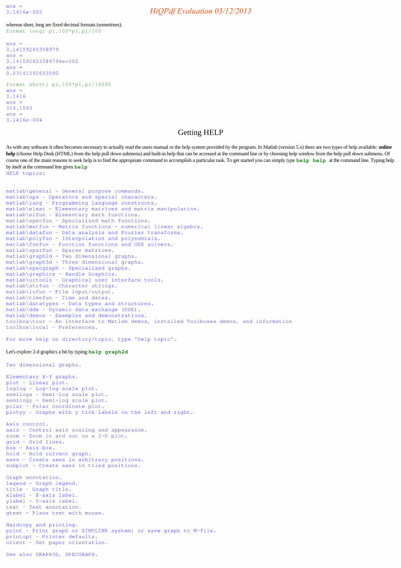
ans = 3.1416e-002

whereas short, long are fixed decimal formats (sometimes). format long; pi,100*pi,pi/100

ans = 3.14159265358979 ans = 3.141592653589794e+002 ans = 0.03141592653590

format short; pi,100*pi,pi/10000 ans = 3.1416 ans = 314.1593 ans = 3.1416e-004

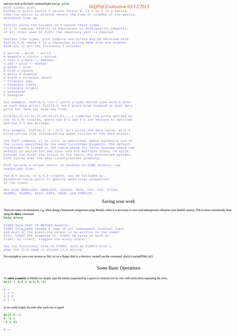
Getting HELP

As with any software it often becomes necessary to actually read the users manual or the help system provided by the program. In Matlab (version 5.x) there are two types of help available: onlinehelp (choose Help Desk (HTML) from the help pull down submenu) and built-in help that can be accessed at the command line or by choosing help window from the help pull down submenu. Ofcourse one of the main reasons to seek help is to find the appropriate command to accomplish a particular task. To get started you can simply type help help at the command line. Typing helpby itself at the command line gives help HELP topics:

matlab\general - General purpose commands. matlab\ops - Operators and special characters. matlab\lang - Programming language constructs. matlab\elmat - Elementary matrices and matrix manipulation. matlab\elfun - Elementary math functions. matlab\specfun - Specialized math functions. matlab\matfun - Matrix functions - numerical linear algebra. matlab\datafun - Data analysis and Fourier transforms. matlab\polyfun - Interpolation and polynomials. matlab\funfun - Function functions and ODE solvers. matlab\sparfun - Sparse matrices. matlab\graph2d - Two dimensional graphs. matlab\graph3d - Three dimensional graphs. matlab\specgraph - Specialized graphs. matlab\graphics - Handle Graphics. matlab\uitools - Graphical user interface tools. matlab\strfun - Character strings. matlab\iofun - File input/output. matlab\timefun - Time and dates. matlab\datatypes - Data types and structures. matlab\dde - Dynamic data exchange (DDE). matlab\demos - Examples and demonstrations. toolbox\tour - An interface to Matlab demos, installed Toolboxes demos, and information toolbox\local - Preferences.

For more help on directory/topic, type "help topic".

Let's explore 2-d graphics a bit by typing help graph2d

Two dimensional graphs.

Elementary X-Y graphs. plot - Linear plot. loglog - Log-log scale plot. semilogx - Semi-log scale plot. semilogy - Semi-log scale plot. polar - Polar coordinate plot. plotyy - Graphs with y tick labels on the left and right.

Axis control. axis - Control axis scaling and appearance. zoom - Zoom in and out on a 2-D plot. grid - Grid lines. box - Axis box. hold - Hold current graph. axes - Create axes in arbitrary positions. subplot - Create axes in tiled positions.

Graph annotation. legend - Graph legend. title - Graph title. xlabel - X-axis label. ylabel - Y-axis label. text - Text annotation. gtext - Place text with mouse.

Hardcopy and printing. print - Print graph or SIMULINK system; or save graph to M-file. printopt - Printer defaults. orient - Set paper orientation.

See also GRAPH3D, SPECGRAPH.

HiQPdf Evaluation 03/12/2013

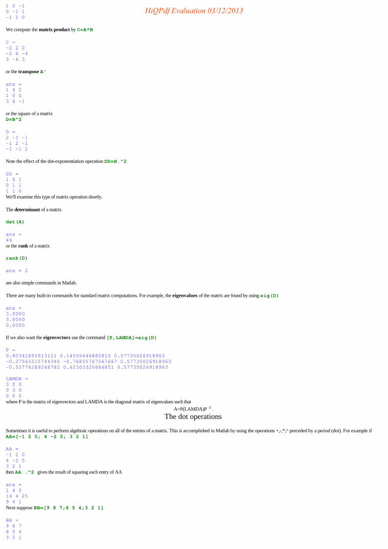
and now look at the basic command plot help plot PLOT Linear plot. PLOT(X,Y) plots vector Y versus vector X. If X or Y is a matrix, then the vector is plotted versus the rows or columns of the matrix, whichever line up.

PLOT(Y) plots the columns of Y versus their index. If Y is complex, PLOT(Y) is equivalent to PLOT(real(Y),imag(Y)). In all other uses of PLOT, the imaginary part is ignored.

Various line types, plot symbols and colors may be obtained with PLOT(X,Y,S) where S is a character string made from one element from any or all the following 3 colunms:

y yellow . point - solid m magenta o circle : dotted c cyan x x-mark -. dashdot r red + plus -- dashed g green * star b blue s square w white d diamond k black v triangle (down) ^ triangle (up) < triangle (left) > triangle (right) p pentagram h hexagram

For example, PLOT(X,Y,'c+:') plots a cyan dotted line with a plus at each data point; PLOT(X,Y,'bd') plots blue diamond at each data point but does not draw any line.

PLOT(X1,Y1,S1,X2,Y2,S2,X3,Y3,S3,...) combines the plots defined by the (X,Y,S) triples, where the X's and Y's are vectors or matrices and the S's are strings.

For example, PLOT(X,Y,'y-',X,Y,'go') plots the data twice, with a solid yellow line interpolating green circles at the data points.

The PLOT command, if no color is specified, makes automatic use of the colors specified by the axes ColorOrder property. The default ColorOrder is listed in the table above for color systems where the default is yellow for one line, and for multiple lines, to cycle through the first six colors in the table. For monochrome systems, PLOT cycles over the axes LineStyleOrder property.

PLOT returns a column vector of handles to LINE objects, one handle per line.

The X,Y pairs, or X,Y,S triples, can be followed by parameter/value pairs to specify additional properties of the lines.

See also SEMILOGX, SEMILOGY, LOGLOG, GRID, CLF, CLC, TITLE, XLABEL, YLABEL, AXIS, AXES, HOLD, and SUBPLOT.

Saving your work

There are many circumstances, e.g. when doing a homework assignment using Matlab, when it is necessary to save and subsequently edit/print your Matlab session. This is most conveniently doneusing the diary command. help diary

DIARY Save text of MATLAB session. DIARY file_name causes a copy of all subsequent terminal input and most of the resulting output to be written on the named file. DIARY OFF suspends it. DIARY ON turns it back on. DIARY, by itself, toggles the diary state.

Use the functional form of DIARY, such as DIARY('file'), when the file name is stored in a string.

For example to save your session as file1.txt on a floppy disk in a directory mystuff use the command: diary('a:\mystuff\file1.txt')

Some Basic Operations

To enter a matrix in Matlab we simply type the entries (separated by a space or comma) row by row with semicolons separating the rows. A=[1 1 3;4 0 6;2,5,-1]

A = 1 1 3 4 0 6 2 5 -1

or we could simply hit enter after each row is typed

B=[1 0 -1 0 -1 1 -1 1 0]

B =

HiQPdf Evaluation 03/12/2013

1 0 -1 0 -1 1 -1 1 0

We compute the matrix product by C=A*B

C = -2 2 0 -2 6 -4 3 -6 3

or the transpose A'

ans = 1 4 2 1 0 5 3 6 -1

or the square of a matrix D=B^2

D = 2 -1 -1 -1 2 -1 -1 -1 2

Note the effect of the dot-exponentiation operation DD=B.^2

DD = 1 0 1 0 1 1 1 1 0 We'll examine this type of matrix operation shortly.

The determinant of a matrix

det(A)

ans = 46 or the rank of a matrix

rank(D)

ans = 2

are also simple commands in Matlab.

There are many built-in commands for standard matrix computations. For example, the eigenvalues of the matrix are found by using eig(D)

ans = 3.0000 3.0000 0.0000

If we also want the eigenvectors use the command [P,LAMDA]=eig(D)

P = 0.80341805013121 0.14555446880815 0.57735026918963 -0.27565515744340 -0.76855767567667 0.57735026918963 -0.52776289268782 0.62300320686851 0.57735026918963

LAMDA = 3 0 0 0 3 0 0 0 0 where P is the matrix of eigenvectors and LAMDA is the diagonal matrix of eigenvalues such that

A=P(LAMDA)P -1 .

The dot operations

Sometimes it is useful to perform algebraic operations on all of the entries of a matrix. This is accomplished in Matlab by using the operations +,-,*,^ preceded by a period (dot). For example ifAA=[-1 2 0; 4 -2 5; 3 2 1]

AA = -1 2 0 4 -2 5 3 2 1 then AA .^2 gives the result of squaring each entry of AA

ans = 1 4 0 16 4 25 9 4 1 Next suppose BB=[9 8 7;6 5 4;3 2 1]

BB = 9 8 7 6 5 4 3 2 1

HiQPdf Evaluation 03/12/2013

and consider the "product" AA.*BB

ans = -9 16 0 24 -10 20 9 4 1 wherein corresponding entries are multiplied.

As another illustration, suppose we want to create an array of values of the function (sin x)/x. Then the following commands create an array of equally spaced points from 0.1 to 1 in x, the values ofsine at each x value in array y, and the ratios using the dot-division operation. x=linspace(.1,1,9),y=sin(x), z=y./x

x = Columns 1 through 7 0.1000 0.2125 0.3250 0.4375 0.5500 0.6625 0.7750 Columns 8 through 9 0.8875 1.0000 y = Columns 1 through 7 0.0998 0.2109 0.3193 0.4237 0.5227 0.6151 0.6997 Columns 8 through 9 0.7755 0.8415 z = Columns 1 through 7 0.9983 0.9925 0.9825 0.9684 0.9503 0.9284 0.9029 Columns 8 through 9 0.8738 0.8415

Creating or identifying matrices

Sometimes it is necessary to identify or define a particular entry of a matrix , or a row, or a column. For example if A

A = -1 2 0 4 -2 5 3 2 1 then

A(3,2)

ans = 2

A(3,: )

ans = 3 2 1

A(:, 2)

ans = 2 -2 2

give the 3,2-entry, 3 rd row, and 2 nd column of the matrix . If we want to delete a row or column of a matrix X=A; use

X(:,3)=[] to delete the third column

X = -1 2 4 -2 3 2

In this context the colon can be viewed as a wildcard. In general, the colon is used in Matlab to identify or define a block of entries in an array. For example to define an array consisting of the first 6integers we use the definition ( u = first:last means create a row vector starting with first, counting by one, and ending on or before last) ints=1:6

ints = 1 2 3 4 5 6

whereas if we want the first 6 odd integers we could increment by 2 using the command

oddints=1:2:11 % gen'l syntax u=first:increment:last

oddints = 1 3 5 7 9 11

Note that oddintegers=1:2:12

oddintegers = 1 3 5 7 9 11

gives the same result.

A standard task in some applications is to create a list of n equally space points between two specified points a and b (with a<b). This is most easily accomplished using the linspace command

HiQPdf Evaluation 03/12/2013

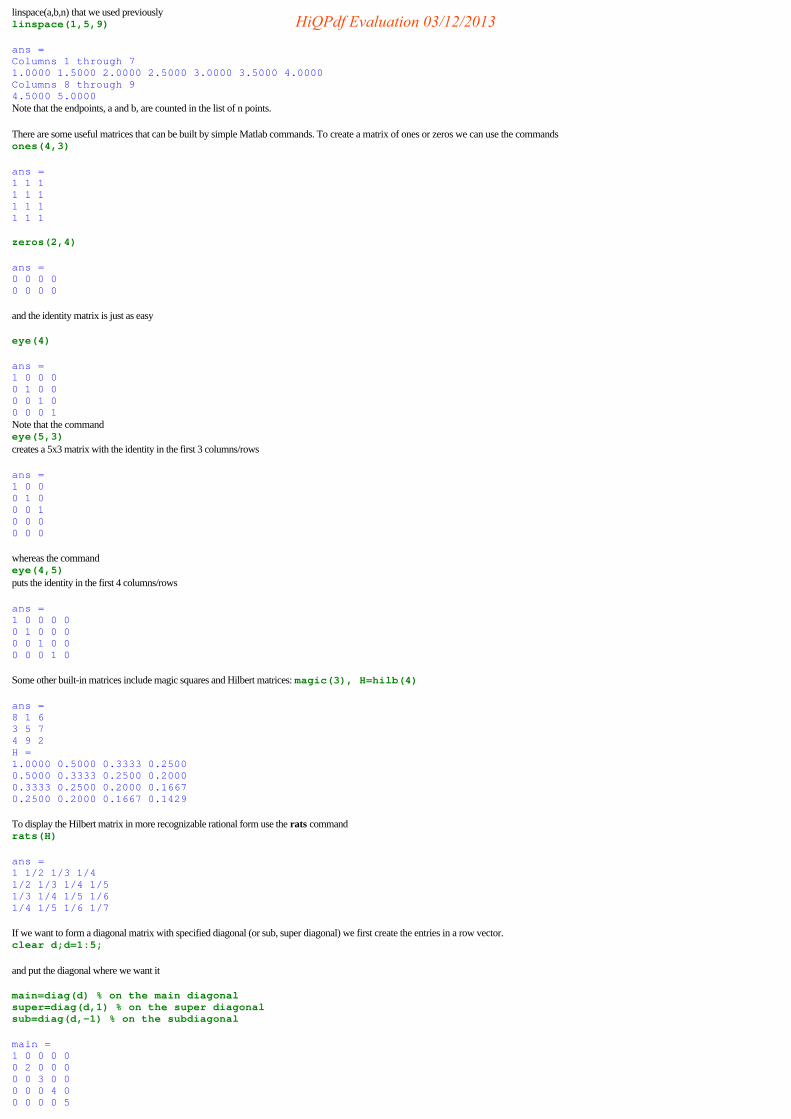
linspace(a,b,n) that we used previously linspace(1,5,9)

ans = Columns 1 through 7 1.0000 1.5000 2.0000 2.5000 3.0000 3.5000 4.0000 Columns 8 through 9 4.5000 5.0000 Note that the endpoints, a and b, are counted in the list of n points.

There are some useful matrices that can be built by simple Matlab commands. To create a matrix of ones or zeros we can use the commands ones(4,3)

ans = 1 1 1 1 1 1 1 1 1 1 1 1

zeros(2,4)

ans = 0 0 0 0 0 0 0 0

and the identity matrix is just as easy

eye(4)

ans = 1 0 0 0 0 1 0 0 0 0 1 0 0 0 0 1 Note that the command eye(5,3) creates a 5x3 matrix with the identity in the first 3 columns/rows

ans = 1 0 0 0 1 0 0 0 1 0 0 0 0 0 0

whereas the command eye(4,5) puts the identity in the first 4 columns/rows

ans = 1 0 0 0 0 0 1 0 0 0 0 0 1 0 0 0 0 0 1 0

Some other built-in matrices include magic squares and Hilbert matrices: magic(3), H=hilb(4)

ans = 8 1 6 3 5 7 4 9 2 H = 1.0000 0.5000 0.3333 0.2500 0.5000 0.3333 0.2500 0.2000 0.3333 0.2500 0.2000 0.1667 0.2500 0.2000 0.1667 0.1429

To display the Hilbert matrix in more recognizable rational form use the rats command rats(H)

ans = 1 1/2 1/3 1/4 1/2 1/3 1/4 1/5 1/3 1/4 1/5 1/6 1/4 1/5 1/6 1/7

If we want to form a diagonal matrix with specified diagonal (or sub, super diagonal) we first create the entries in a row vector. clear d;d=1:5;

and put the diagonal where we want it

main=diag(d) % on the main diagonal super=diag(d,1) % on the super diagonal sub=diag(d,-1) % on the subdiagonal

main = 1 0 0 0 0 0 2 0 0 0 0 0 3 0 0 0 0 0 4 0 0 0 0 0 5

HiQPdf Evaluation 03/12/2013

super = 0 1 0 0 0 0 0 0 2 0 0 0 0 0 0 3 0 0 0 0 0 0 4 0 0 0 0 0 0 5 0 0 0 0 0 0 sub = 0 0 0 0 0 0 1 0 0 0 0 0 0 2 0 0 0 0 0 0 3 0 0 0 0 0 0 4 0 0 0 0 0 0 5 0

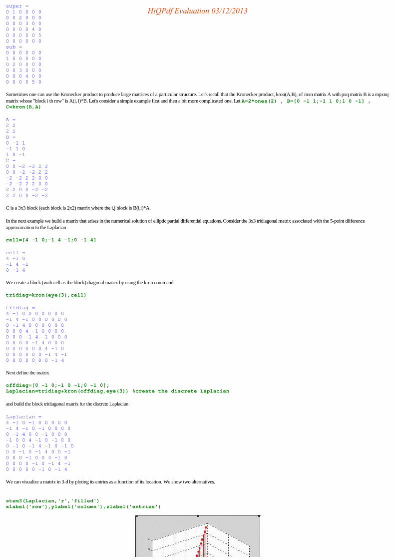
Sometimes one can use the Kronecker product to produce large matrices of a particular structure. Let's recall that the Kronecker product, kron(A,B), of mxn matrix A with pxq matrix B is a mpxnqmatrix whose "block i th row" is A(i, i)*B. Let's consider a simple example first and then a bit more complicated one. Let A=2*ones(2) , B=[0 -1 1;-1 1 0;1 0 -1] ,C=kron(B,A)

A = 2 2 2 2 B = 0 -1 1 -1 1 0 1 0 -1 C = 0 0 -2 -2 2 2 0 0 -2 -2 2 2 -2 -2 2 2 0 0 -2 -2 2 2 0 0 2 2 0 0 -2 -2 2 2 0 0 -2 -2

C is a 3x3 block (each block is 2x2) matrix where the i,j block is B(i,i)*A.

In the next example we build a matrix that arises in the numerical solution of elliptic partial differential equations. Consider the 3x3 tridiagonal matrix associated with the 5-point differenceapproximation to the Laplacian

cell=[4 -1 0;-1 4 -1;0 -1 4]

cell = 4 -1 0 -1 4 -1 0 -1 4

We create a block (with cell as the block) diagonal matrix by using the kron command

tridiag=kron(eye(3),cell)

tridiag = 4 -1 0 0 0 0 0 0 0 -1 4 -1 0 0 0 0 0 0 0 -1 4 0 0 0 0 0 0 0 0 0 4 -1 0 0 0 0 0 0 0 -1 4 -1 0 0 0 0 0 0 0 -1 4 0 0 0 0 0 0 0 0 0 4 -1 0 0 0 0 0 0 0 -1 4 -1 0 0 0 0 0 0 0 -1 4

Next define the matrix

offdiag=[0 -1 0;-1 0 -1;0 -1 0]; Laplacian=tridiag+kron(offdiag,eye(3)) %create the discrete Laplacian

and build the block tridiagonal matrix for the discrete Laplacian

Laplacian = 4 -1 0 -1 0 0 0 0 0 -1 4 -1 0 -1 0 0 0 0 0 -1 4 0 0 -1 0 0 0 -1 0 0 4 -1 0 -1 0 0 0 -1 0 -1 4 -1 0 -1 0 0 0 -1 0 -1 4 0 0 -1 0 0 0 -1 0 0 4 -1 0 0 0 0 0 -1 0 -1 4 -1 0 0 0 0 0 -1 0 -1 4

We can visualize a matrix in 3-d by ploting its entries as a function of its location. We show two alternatives.

stem3(Laplacian,'r','filled') xlabel('row'),ylabel('column'),zlabel('entries')

HiQPdf Evaluation 03/12/2013

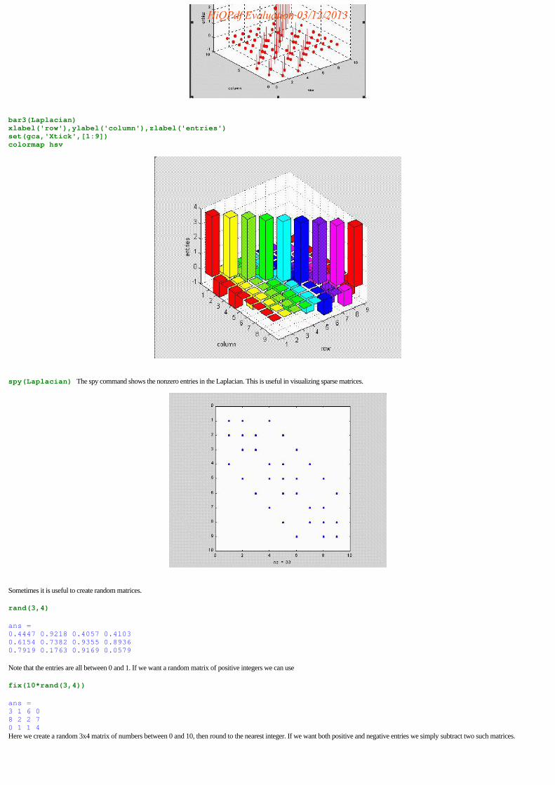
bar3(Laplacian) xlabel('row'),ylabel('column'),zlabel('entries') set(gca,'Xtick',[1:9]) colormap hsv

spy(Laplacian) The spy command shows the nonzero entries in the Laplacian. This is useful in visualizing sparse matrices.

Sometimes it is useful to create random matrices.

rand(3,4)

ans = 0.4447 0.9218 0.4057 0.4103 0.6154 0.7382 0.9355 0.8936 0.7919 0.1763 0.9169 0.0579

Note that the entries are all between 0 and 1. If we want a random matrix of positive integers we can use

fix(10*rand(3,4))

ans = 3 1 6 0 8 2 2 7 0 1 1 4 Here we create a random 3x4 matrix of numbers between 0 and 10, then round to the nearest integer. If we want both positive and negative entries we simply subtract two such matrices.

HiQPdf Evaluation 03/12/2013

2D Graphics

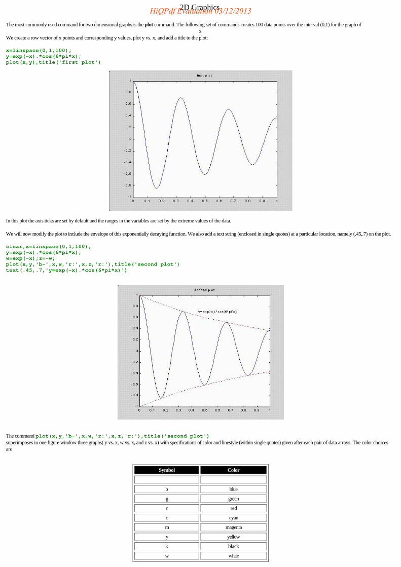
The most commonly used command for two dimensional graphs is the plot command. The following set of commands creates 100 data points over the interval (0,1) for the graph of x

We create a row vector of x points and corresponding y values, plot y vs. x, and add a title to the plot:

x=linspace(0,1,100); y=exp(-x).*cos(6*pi*x); plot(x,y),title('first plot')

In this plot the axis ticks are set by default and the ranges in the variables are set by the extreme values of the data.

We will now modify the plot to include the envelope of this exponentially decaying function. We also add a text string (enclosed in single quotes) at a particular location, namely (.45,.7) on the plot.

clear;x=linspace(0,1,100); y=exp(-x).*cos(6*pi*x); w=exp(-x);z=-w; plot(x,y,'b-',x,w,'r:',x,z,'r:'),title('second plot') text(.45,.7,'y=exp(-x).*cos(6*pi*x)')

The command plot(x,y,'b-',x,w,'r:',x,z,'r:'),title('second plot') superimposes in one figure window three graphs( y vs. x, w vs. x, and z vs. x) with specifications of color and linestyle (within single quotes) given after each pair of data arrays. The color choicesare

Symbol Color

b blue

g green

r red

c cyan

m magenta

y yellow

k black

w white

HiQPdf Evaluation 03/12/2013

and the linestyle choices are

Symbol Linestyle

- solid line

: dotted line

-. dash-dot line

-- dashed line

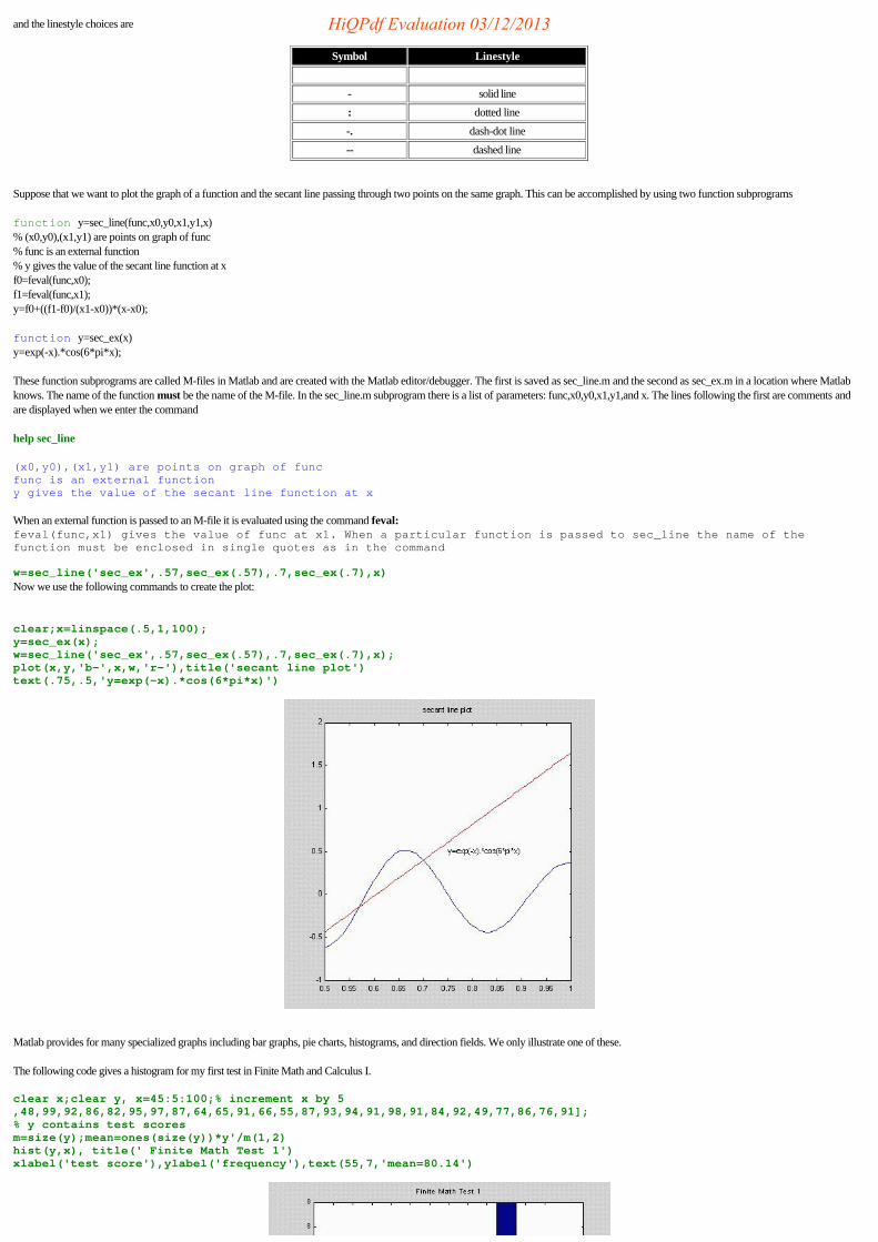
Suppose that we want to plot the graph of a function and the secant line passing through two points on the same graph. This can be accomplished by using two function subprograms

function y=sec_line(func,x0,y0,x1,y1,x) % (x0,y0),(x1,y1) are points on graph of func % func is an external function % y gives the value of the secant line function at x f0=feval(func,x0); f1=feval(func,x1); y=f0+((f1-f0)/(x1-x0))*(x-x0);

function y=sec_ex(x) y=exp(-x).*cos(6*pi*x);

These function subprograms are called M-files in Matlab and are created with the Matlab editor/debugger. The first is saved as sec_line.m and the second as sec_ex.m in a location where Matlabknows. The name of the function must be the name of the M-file. In the sec_line.m subprogram there is a list of parameters: func,x0,y0,x1,y1,and x. The lines following the first are comments andare displayed when we enter the command

help sec_line

(x0,y0),(x1,y1) are points on graph of func func is an external function y gives the value of the secant line function at x

When an external function is passed to an M-file it is evaluated using the command feval: feval(func,x1) gives the value of func at x1. When a particular function is passed to sec_line the name of thefunction must be enclosed in single quotes as in the command

w=sec_line('sec_ex',.57,sec_ex(.57),.7,sec_ex(.7),x) Now we use the following commands to create the plot:

clear;x=linspace(.5,1,100); y=sec_ex(x); w=sec_line('sec_ex',.57,sec_ex(.57),.7,sec_ex(.7),x); plot(x,y,'b-',x,w,'r-'),title('secant line plot') text(.75,.5,'y=exp(-x).*cos(6*pi*x)')

Matlab provides for many specialized graphs including bar graphs, pie charts, histograms, and direction fields. We only illustrate one of these.

The following code gives a histogram for my first test in Finite Math and Calculus I.

clear x;clear y, x=45:5:100;% increment x by 5 ,48,99,92,86,82,95,97,87,64,65,91,66,55,87,93,94,91,98,91,84,92,49,77,86,76,91]; % y contains test scores m=size(y);mean=ones(size(y))*y'/m(1,2) hist(y,x), title(' Finite Math Test 1') xlabel('test score'),ylabel('frequency'),text(55,7,'mean=80.14')

HiQPdf Evaluation 03/12/2013

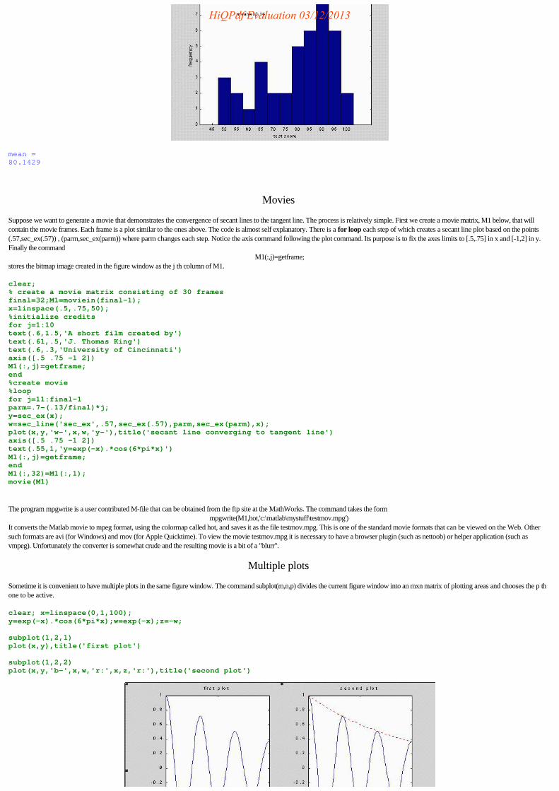
mean = 80.1429

Movies

Suppose we want to generate a movie that demonstrates the convergence of secant lines to the tangent line. The process is relatively simple. First we create a movie matrix, M1 below, that willcontain the movie frames. Each frame is a plot similar to the ones above. The code is almost self explanatory. There is a for loop each step of which creates a secant line plot based on the points(.57,sec_ex(.57)) , (parm,sec_ex(parm)) where parm changes each step. Notice the axis command following the plot command. Its purpose is to fix the axes limits to [.5,.75] in x and [-1,2] in y.Finally the command

M1(:,j)=getframe;stores the bitmap image created in the figure window as the j th column of M1.

clear; % create a movie matrix consisting of 30 frames final=32;M1=moviein(final-1); x=linspace(.5,.75,50); %initialize credits for j=1:10 text(.6,1.5,'A short film created by') text(.61,.5,'J. Thomas King') text(.6,.3,'University of Cincinnati') axis([.5 .75 -1 2]) M1(:,j)=getframe; end %create movie %loop for j=11:final-1 parm=.7-(.13/final)*j; y=sec_ex(x); w=sec_line('sec_ex',.57,sec_ex(.57),parm,sec_ex(parm),x); plot(x,y,'w-',x,w,'y-'),title('secant line converging to tangent line') axis([.5 .75 -1 2]) text(.55,1,'y=exp(-x).*cos(6*pi*x)') M1(:,j)=getframe; end M1(:,32)=M1(:,1); movie(M1)

The program mpgwrite is a user contributed M-file that can be obtained from the ftp site at the MathWorks. The command takes the form mpgwrite(M1,hot,'c:\matlab\mystuff\testmov.mpg')

It converts the Matlab movie to mpeg format, using the colormap called hot, and saves it as the file testmov.mpg. This is one of the standard movie formats that can be viewed on the Web. Othersuch formats are avi (for Windows) and mov (for Apple Quicktime). To view the movie testmov.mpg it is necessary to have a browser plugin (such as nettoob) or helper application (such asvmpeg). Unfortunately the converter is somewhat crude and the resulting movie is a bit of a "blurr".

Multiple plots

Sometime it is convenient to have multiple plots in the same figure window. The command subplot(m,n,p) divides the current figure window into an mxn matrix of plotting areas and chooses the p thone to be active.

clear; x=linspace(0,1,100); y=exp(-x).*cos(6*pi*x);w=exp(-x);z=-w;

subplot(1,2,1) plot(x,y),title('first plot')

subplot(1,2,2) plot(x,y,'b-',x,w,'r:',x,z,'r:'),title('second plot')

HiQPdf Evaluation 03/12/2013

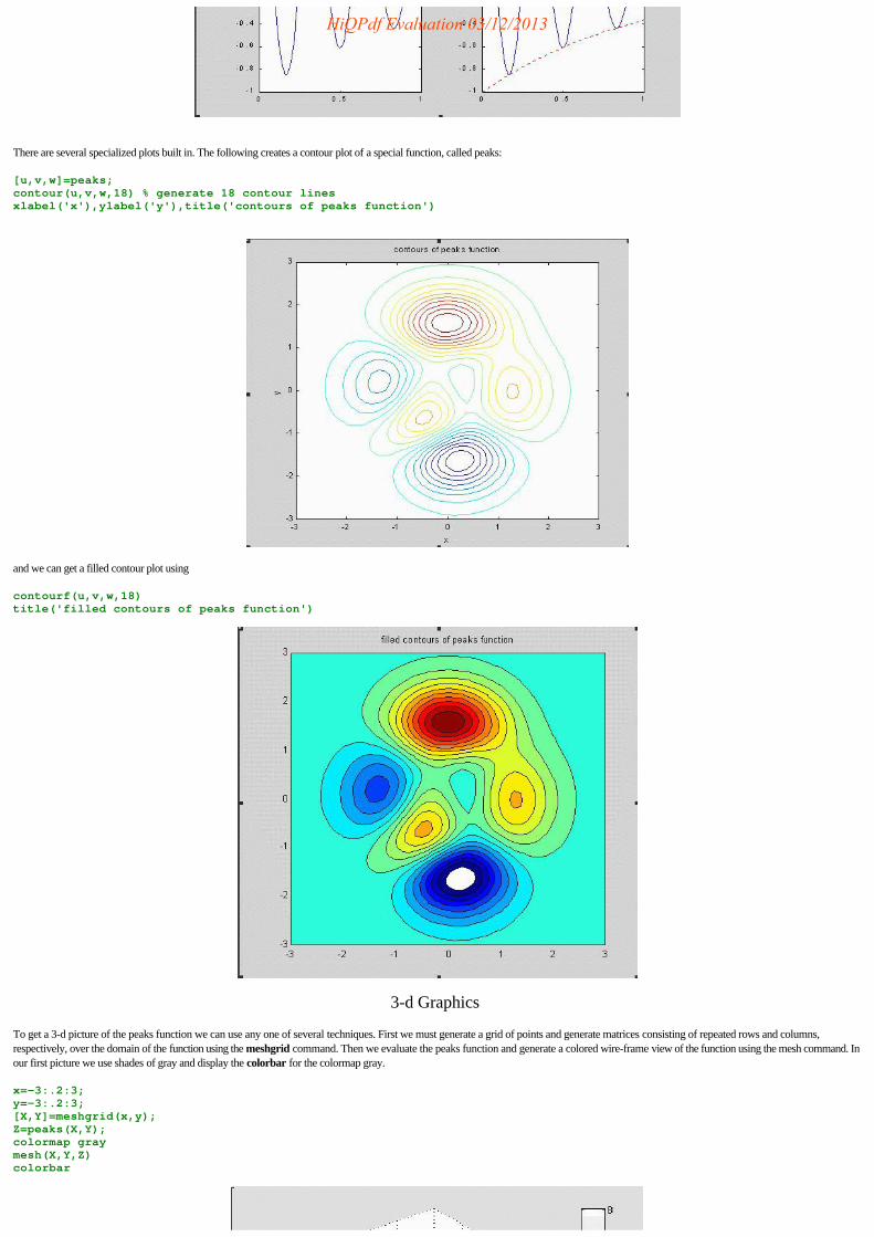
There are several specialized plots built in. The following creates a contour plot of a special function, called peaks:

[u,v,w]=peaks; contour(u,v,w,18) % generate 18 contour lines xlabel('x'),ylabel('y'),title('contours of peaks function')

and we can get a filled contour plot using

contourf(u,v,w,18) title('filled contours of peaks function')

3-d Graphics

To get a 3-d picture of the peaks function we can use any one of several techniques. First we must generate a grid of points and generate matrices consisting of repeated rows and columns,respectively, over the domain of the function using the meshgrid command. Then we evaluate the peaks function and generate a colored wire-frame view of the function using the mesh command. Inour first picture we use shades of gray and display the colorbar for the colormap gray.

x=-3:.2:3; y=-3:.2:3; [X,Y]=meshgrid(x,y); Z=peaks(X,Y); colormap gray mesh(X,Y,Z) colorbar

HiQPdf Evaluation 03/12/2013

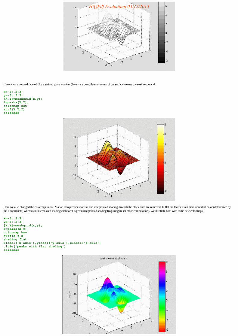
If we want a colored faceted like a stained glass window (facets are quadrilaterals) view of the surface we use the surf command.

x=-3:.2:3; y=-3:.2:3; [X,Y]=meshgrid(x,y); Z=peaks(X,Y); colormap hot surf(X,Y,Z) colorbar

Here we also changed the colormap to hot. Matlab also provides for flat and interpolated shading. In each the black lines are removed. In flat the facets retain their individual color (determined bythe z coordinate) whereas in interpolated shading each facet is given interpolated shading (requiring much more computation). We illustrate both with some new colormaps.

x=-3:.2:3; y=-3:.2:3; [X,Y]=meshgrid(x,y); Z=peaks(X,Y); colormap hsv surf(X,Y,Z) shading flat xlabel('x-axis'),ylabel('y-axis'),zlabel('z-axis') title('peaks with flat shading') colorbar

HiQPdf Evaluation 03/12/2013

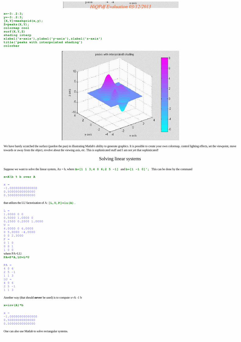
x=-3:.2:3; y=-3:.2:3; [X,Y]=meshgrid(x,y); Z=peaks(X,Y); colormap cool surf(X,Y,Z) shading interp xlabel('x-axis'),ylabel('y-axis'),zlabel('z-axis') title('peaks with interpolated shading') colorbar

We have barely scratched the surface (pardon the pun) in illustrating Matlab's ability to generate graphics. It is possible to create your own colormap, control lighting effects, set the viewpoint, movetowards or away from the object, revolve about the viewing axis, etc. This is sophisticated stuff and I am not yet that sophisticated!

Solving linear systems

Suppose we want to solve the linear system, Ax = b, where A=[1 1 3;4 0 6;2 5 -1] and b=[1 -1 0]'; This can be done by the command

x=A\b % b over A

x = -1.00000000000000 0.50000000000000 0.50000000000000

that utilizes the LU factorization of A: [L,U,P]=lu(A).

L = 1.0000 0 0 0.5000 1.0000 0 0.2500 0.2000 1.0000 U = 4.0000 0 6.0000 0 5.0000 -4.0000 0 0 2.3000 P = 0 1 0 0 0 1 1 0 0 where PA=LU: PA=P*A,LU=L*U

PA = 4 0 6 2 5 -1 1 1 3 LU = 4 0 6 2 5 -1 1 1 3

Another way (that should never be used) is to compute x=A -1 b

x=inv(A)*b

x = -1.00000000000000 0.50000000000000 0.50000000000000

One can also use Matlab to solve rectangular systems.

HiQPdf Evaluation 03/12/2013

Working with the rref of a matrix

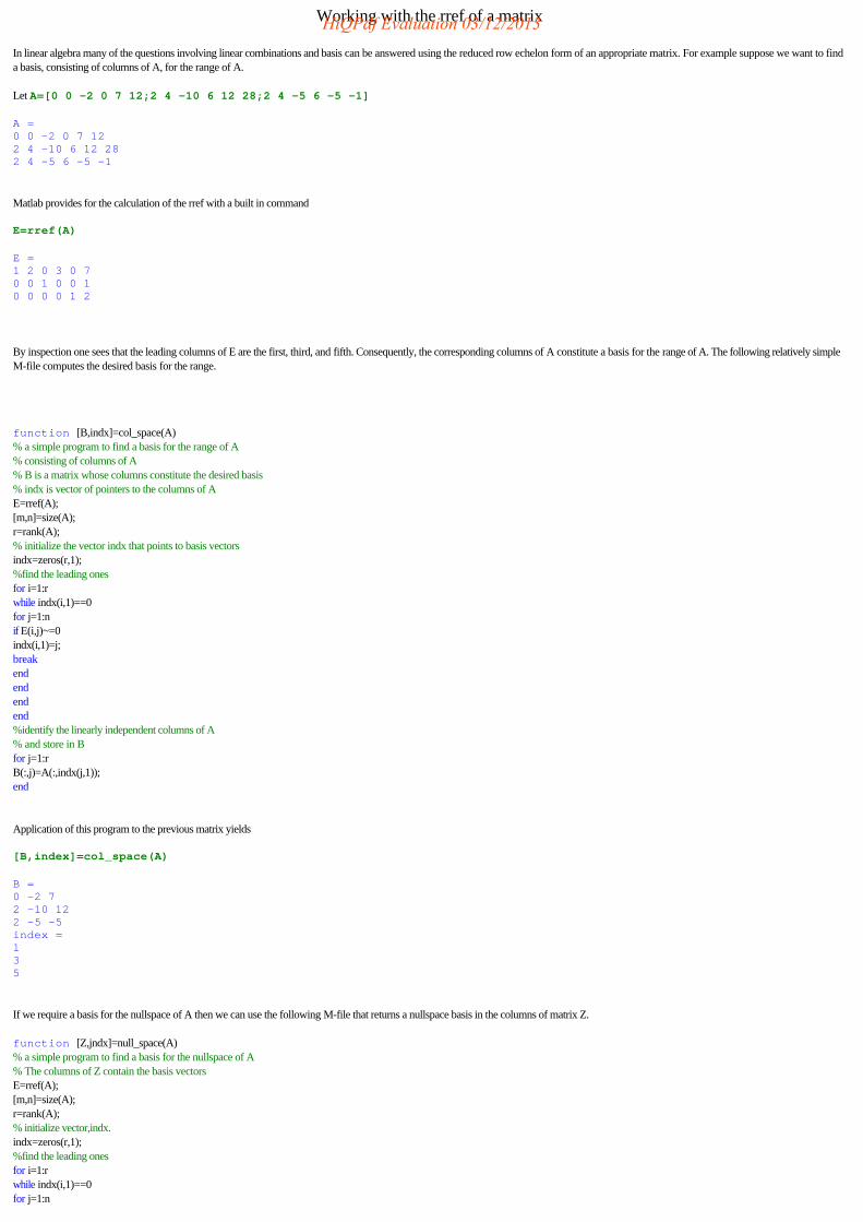
In linear algebra many of the questions involving linear combinations and basis can be answered using the reduced row echelon form of an appropriate matrix. For example suppose we want to finda basis, consisting of columns of A, for the range of A.

Let A=[0 0 -2 0 7 12;2 4 -10 6 12 28;2 4 -5 6 -5 -1]

A = 0 0 -2 0 7 12 2 4 -10 6 12 28 2 4 -5 6 -5 -1

Matlab provides for the calculation of the rref with a built in command

E=rref(A)

E = 1 2 0 3 0 7 0 0 1 0 0 1 0 0 0 0 1 2

By inspection one sees that the leading columns of E are the first, third, and fifth. Consequently, the corresponding columns of A constitute a basis for the range of A. The following relatively simpleM-file computes the desired basis for the range.

function [B,indx]=col_space(A) % a simple program to find a basis for the range of A % consisting of columns of A % B is a matrix whose columns constitute the desired basis % indx is vector of pointers to the columns of A E=rref(A); [m,n]=size(A); r=rank(A); % initialize the vector indx that points to basis vectors indx=zeros(r,1); %find the leading ones for i=1:r while indx(i,1)==0 for j=1:n if E(i,j)~=0 indx(i,1)=j; break end end end end %identify the linearly independent columns of A % and store in B for j=1:r B(:,j)=A(:,indx(j,1)); end

Application of this program to the previous matrix yields

[B,index]=col_space(A)

B = 0 -2 7 2 -10 12 2 -5 -5 index = 1 3 5

If we require a basis for the nullspace of A then we can use the following M-file that returns a nullspace basis in the columns of matrix Z.

function [Z,jndx]=null_space(A) % a simple program to find a basis for the nullspace of A % The columns of Z contain the basis vectors E=rref(A); [m,n]=size(A); r=rank(A); % initialize vector,indx. indx=zeros(r,1); %find the leading ones for i=1:r while indx(i,1)==0 for j=1:n

HiQPdf Evaluation 03/12/2013

if E(i,j)~=0 indx(i,1)=j; break end end end end %initialize jndx=zeros(n-r,1); count=1; %determine the arbitrary variables for j=1:n flag=1; for i=1:r if indx(i,1)==j flag=0; break else end end if flag~=0 jndx(count,1)=j;count=count+1; end end %find the basis vectors and store in Z Z=zeros(n,n-r); for j=1:n-r jj=jndx(j,1);Z(jj,j)=1; for i=1:r Z(indx(i,1),j)= -E(i,jj); end end

When applied to the previous matrix there results:

W=null_space(A)

W = -2 -3 -7 1 0 0 0 0 -1 0 1 0 0 0 -2 0 0 1

It is obvious that these three vectors are linearly independent and since

A*W

ans = 0 0 0 0 0 0 0 0 0

we see that each vector is in the nullspace of A.

Example: Solving the simple pendulum equation

Consider a pendulum of length L having a "bob" of mass m:

where we assume the rod is rigid and has negligible mass compared to the bob. We also suppose there is no friction or air resistence. Using Newton's 2 nd law one finds the following differentialequation for the angular displacement, S (t):

HiQPdf Evaluation 03/12/2013

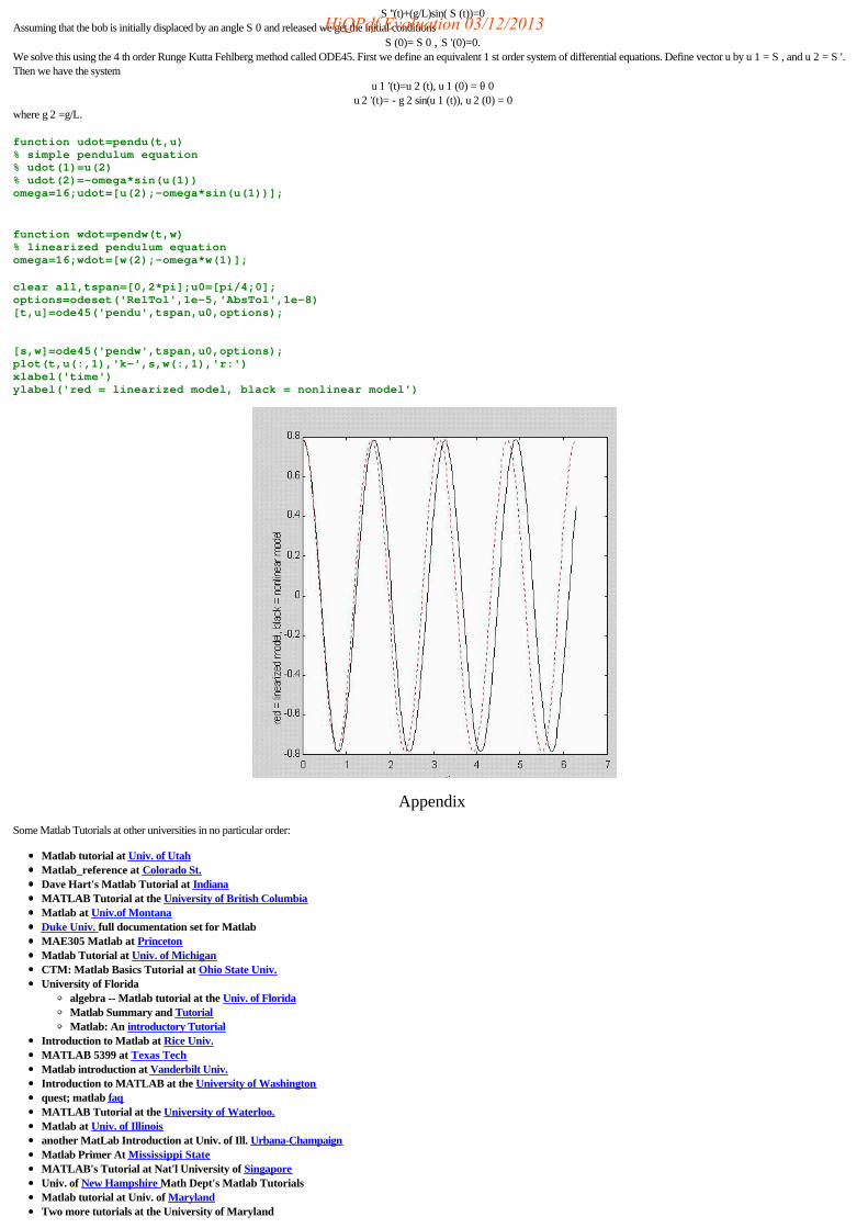
S ''(t)+(g/L)sin( S (t))=0 Assuming that the bob is initially displaced by an angle S 0 and released we get the initial conditions

S (0)= S 0 , S '(0)=0. We solve this using the 4 th order Runge Kutta Fehlberg method called ODE45. First we define an equivalent 1 st order system of differential equations. Define vector u by u 1 = S , and u 2 = S '.Then we have the system

u 1 '(t)=u 2 (t), u 1 (0) = q 0 u 2 '(t)= - g 2 sin(u 1 (t)), u 2 (0) = 0

where g 2 =g/L.

function udot=pendu(t,u) % simple pendulum equation % udot(1)=u(2) % udot(2)=-omega*sin(u(1)) omega=16;udot=[u(2);-omega*sin(u(1))];

function wdot=pendw(t,w) % linearized pendulum equation omega=16;wdot=[w(2);-omega*w(1)];

clear all,tspan=[0,2*pi];u0=[pi/4;0]; options=odeset('RelTol',1e-5,'AbsTol',1e-8) [t,u]=ode45('pendu',tspan,u0,options);

[s,w]=ode45('pendw',tspan,u0,options); plot(t,u(:,1),'k-',s,w(:,1),'r:') xlabel('time') ylabel('red = linearized model, black = nonlinear model')

Appendix

Some Matlab Tutorials at other universities in no particular order:

Matlab tutorial at Univ. of UtahMatlab_reference at Colorado St.Dave Hart's Matlab Tutorial at IndianaMATLAB Tutorial at the University of British ColumbiaMatlab at Univ.of MontanaDuke Univ. full documentation set for MatlabMAE305 Matlab at PrincetonMatlab Tutorial at Univ. of MichiganCTM: Matlab Basics Tutorial at Ohio State Univ.University of Florida

algebra -- Matlab tutorial at the Univ. of FloridaMatlab Summary and TutorialMatlab: An introductory Tutorial

Introduction to Matlab at Rice Univ.MATLAB 5399 at Texas TechMatlab introduction at Vanderbilt Univ.Introduction to MATLAB at the University of Washingtonquest; matlab faqMATLAB Tutorial at the University of Waterloo.Matlab at Univ. of Illinoisanother MatLab Introduction at Univ. of Ill. Urbana-ChampaignMatlab Primer At Mississippi StateMATLAB's Tutorial at Nat'l University of SingaporeUniv. of New Hampshire Math Dept's Matlab TutorialsMatlab tutorial at Univ. of MarylandTwo more tutorials at the University of Maryland

HiQPdf Evaluation 03/12/2013

1. Matlab tutorial - 12. Matlab tutorial - 2

Matlab Primer,3 rd ed. by Kermit Sigmon at U. Fla, Postscript fileTutorial at St. Olaf

Other Matlab related links

The makers of MATLABThe MathWorks, Inc - Matlab FAQINDEX of user-contributed files on ftp.mathworks.comWelcome to MATLAB In EducationThe MATLAB NewsgroupMATLAB Project

HiQPdf Evaluation 03/12/2013