Matlab Fundamentals

Appendix AMatlab Fundamentals

This appendix provides an overview of Matlab1 mathematical software, widely usedin scientific computation applications to simulate physical systems, run computa-tional algorithms, as well as perform comprehensive data analysis and visualisation.Optional toolboxes extend Matlab functionality to specialised applications includ-ing neural networks, signal processing, bioinformatics, system identification, imageprocessing and systems biology.

A.1 Matlab Overview

Matlab provides an interpreter environment for executing an extensive library ofin-built mathematical commands, as well as user-defined code scripts and functions.This section provides an overview of the Matlab interface and basic functionality.

A.1.1 User Interface

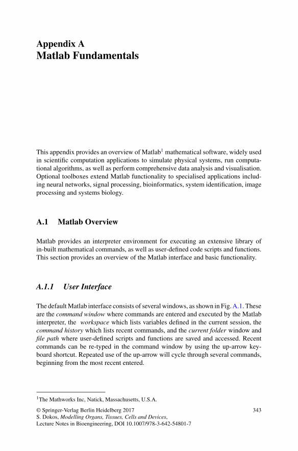
The defaultMatlab interface consists of several windows, as shown in Fig.A.1. Theseare the command window where commands are entered and executed by the Matlabinterpreter, the workspace which lists variables defined in the current session, thecommand history which lists recent commands, and the current folder window andfile path where user-defined scripts and functions are saved and accessed. Recentcommands can be re-typed in the command window by using the up-arrow key-board shortcut. Repeated use of the up-arrow will cycle through several commands,beginning from the most recent entered.

1The Mathworks Inc, Natick, Massachusetts, U.S.A.

© Springer-Verlag Berlin Heidelberg 2017S. Dokos, Modelling Organs, Tissues, Cells and Devices,Lecture Notes in Bioengineering, DOI 10.1007/978-3-642-54801-7

343

344 Appendix A: Matlab Fundamentals

Fig. A.1 Default Matlab interface. The command window represents the main work area wherecommands are entered for execution by the Matlab interpreter. The workspace window displayscurrent variables, the command history shows recent commands entered, and the current folderwindow specified by the file path lists local files

A.1.2 Working with Variables and Arrays

Variables do not need to be declared first: simply assign their value directly. Forexample, the following commands entered in the command window:

r = 2;

c = 2*pi*r;

will create the variables r and c in the current workspace and assign their valuesto 2 and 2 × π × 2 = 4π respectively (note that pi is the in-built Matlab constantfor π ≈ 3.1416). Note that each command ends with a semicolon. Although notstrictly necessary, the semicolon prevents command results from being echoed in thecommand window.

To define an array, values can be entered element by element, as in the following:

x = [2,3,1,0,0];

y = [1;2;3;4;5];

A = [1,0;0,1];

which define x to be a five-element row array, y a five-element column array, and Aas the 2 × 2 identity matrix. The subsequent command

Appendix A: Matlab Fundamentals 345

d = x*y;

would perform array multiplication of a row and column vector, yielding the scalard = 11. Reversing the order of the arrays in the command E = y*x would assign a5 × 5 matrix to E.

Individual elements of the above arrays can be accessed using commands suchas x(1) (returning a value of 2) and A(1,2) (returning a value of 0). To appendelements to existing arrays, use commands like

z = [x,3];

w = [y;8];

which add extra elements of value 3 and 8 to the end of the above-defined arraysx andy respectively. Note that a comma appends to rows, whilst a semi-colon appends tocolumns. Similar principles applywhen concatenating two-arrays. Thus, for example

z = [x,x];

w = [y;y];

would double the length of both x and y defined above.Arrays can also be defined using

x = 0:0.001:1;

which creates a row array of 1001 uniformly-spaced elements, 0 as the first and 1as the last, in increments of 0.001. An alternative is to use Matlab’s linspacefunction:

x = linspace(0,1,1001);

which yields the same result. Note that this function takes three arguments, the firstand last values of the array, and the total number of elements.

To square each element of x, use the .ˆ exponent operator which acts on eachelement of x individually:

y = x.ˆ2;

Analogous element by element array operators also defined for multiplication (.*)and division (./). Thus, for example, the following sequence of commands:

A = [1,2;3,4];

B = [5,6;7,8];


C = A*B;

D = A.*B;

E = A/B;

F = A./B;

would yield

C =[19 2243 50

], D =

[5 1221 32

], E =

[3 −22 −1

], F =

[0.2 0.3333

0.4286 0.5

].

Note that the division operator (/) for calculating E denotes matrix division, suchthat A/B = A*inv(B) where inv(B) is the inverse of matrix B.

In addition to real number data types,Matlab allows other variable types includingstrings and complex numbers. For example, the commands

a = ‘This is some text’;

b = complex(1,2);

define a and b to be string and complex data types respectively.A short list of basic Matlab operators and functions is given in TableA.1. More

comprehensive documentation onMatlab operators, functions and advanced featurescan be found in the in-built documentation, which can be accessed from the commandwindow using

doc matlab

Help on any command can be obtained in the command window by typing helpfollowed by the command, e.g.

help linspace

Typing doc followed by the command will display html-formatted documentationinstead:

doc linspace

A.1.3 Matlab Programming

Matlab provides an extensive set of high-level programming features for implement-ing complex automated numerical computations and algorithms.


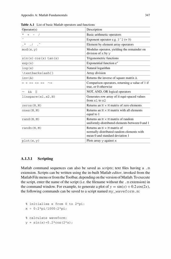
Table A.1 List of basic Matlab operators and functions

Operator(s) Description

* + - / Basic arithmetic operators

ˆ Exponent operator e.g. 3ˆ2 (= 9)

.* ./ .ˆ Element by element array operators

mod(x,y) Modulus operator, yielding the remainder ondivision of x by y

sin(x) cos(x) tan(x) Trigonometric functions

exp(x) Exponential function ex

log(x) Natural logarithm

\textbackslash{} Array division

inv(A) Returns the inverse of square matrix A

> < >= <= == ∼= Comparison operators, returning a value of 1 iftrue, or 0 otherwise

∼ && || NOT, AND, OR logical operators

linspace(x1,x2,N) Generates row array of N equi-spaced valuesfrom x1 to x2

zeros(N,M) Returns an N × M matrix of zero elements

ones(N,M) Returns an N × M matrix with all elementsequal to 1

rand(N,M) Returns an N × M matrix of randomuniformly-distributed elements between 0 and 1

randn(N,M) Returns an N × M matrix ofnormally-distributed random elements withmean 0 and standard deviation 1

plot(x,y) Plots array y against x

A.1.3.1 Scripting

Matlab command sequences can also be saved as scripts; text files having a .mextension. Scripts can be written using the in-built Matlab editor, invoked from theMatlab Filemenu or from theToolbar, depending on the version ofMatlab. To executethe script, enter the name of the script (i.e. the filename without the .m extension) inthe command window. For example, to generate a plot of y = sin(x) + 0.2 cos(2x),the following commands can be saved to a script named my_waveform.m:

% initialise x from 0 to 2*pi:

x = 0:2*pi/1000:2*pi;

% calculate waveform:

y = sin(x)+0.2*cos(2*x);


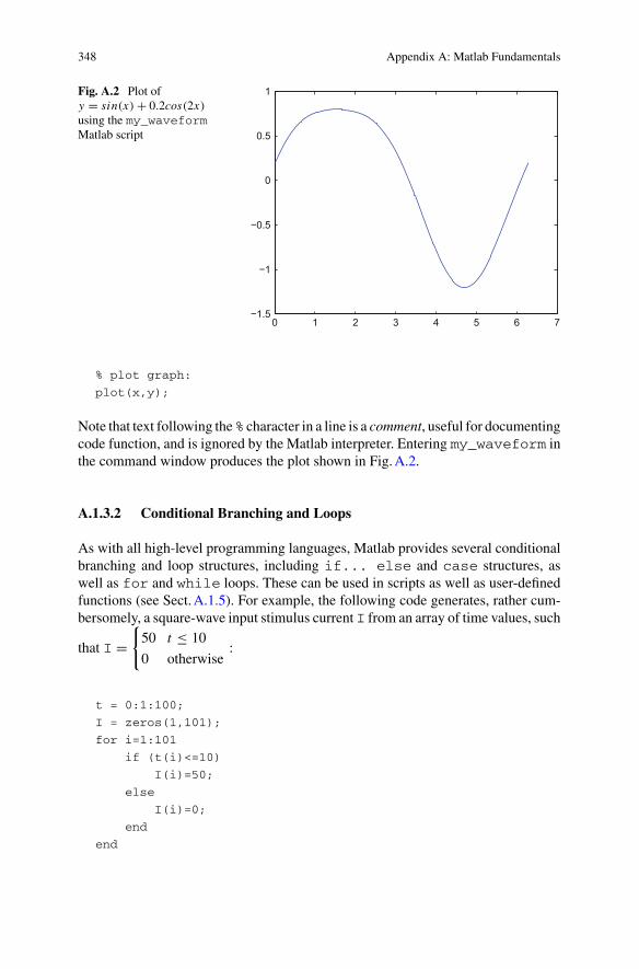
Fig. A.2 Plot ofy = sin(x) + 0.2cos(2x)using the my_waveformMatlab script

0 1 2 3 4 5 6 7−1.5

−1

−0.5

0

0.5

1

% plot graph:

plot(x,y);

Note that text following the% character in a line is a comment, useful for documentingcode function, and is ignored by the Matlab interpreter. Entering my_waveform inthe command window produces the plot shown in Fig.A.2.

A.1.3.2 Conditional Branching and Loops

As with all high-level programming languages, Matlab provides several conditionalbranching and loop structures, including if... else and case structures, aswell as for and while loops. These can be used in scripts as well as user-definedfunctions (see Sect.A.1.5). For example, the following code generates, rather cum-bersomely, a square-wave input stimulus current I from an array of time values, such

that I ={50 t ≤ 10

0 otherwise:

t = 0:1:100;

I = zeros(1,101);

for i=1:101

if (t(i)<=10)

I(i)=50;

else

I(i)=0;

end

end


Note that the same result could be generated using the far more compact code:

t = 0:1:100;

I = 50*(t<=10);

A.1.3.3 Code Debugging

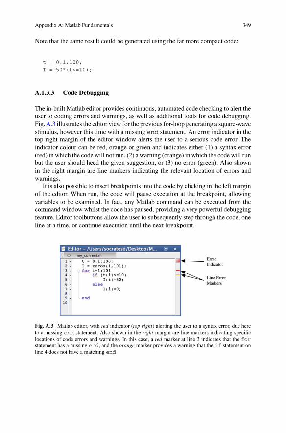
The in-built Matlab editor provides continuous, automated code checking to alert theuser to coding errors and warnings, as well as additional tools for code debugging.Fig.A.3 illustrates the editor view for the previous for-loop generating a square-wavestimulus, however this time with a missing end statement. An error indicator in thetop right margin of the editor window alerts the user to a serious code error. Theindicator colour can be red, orange or green and indicates either (1) a syntax error(red) in which the code will not run, (2) a warning (orange) in which the code will runbut the user should heed the given suggestion, or (3) no error (green). Also shownin the right margin are line markers indicating the relevant location of errors andwarnings.

It is also possible to insert breakpoints into the code by clicking in the left marginof the editor. When run, the code will pause execution at the breakpoint, allowingvariables to be examined. In fact, any Matlab command can be executed from thecommand window whilst the code has paused, providing a very powerful debuggingfeature. Editor toolbuttons allow the user to subsequently step through the code, oneline at a time, or continue execution until the next breakpoint.

Fig. A.3 Matlab editor, with red indicator (top right) alerting the user to a syntax error, due hereto a missing end statement. Also shown in the right margin are line markers indicating specificlocations of code errors and warnings. In this case, a red marker at line 3 indicates that the forstatement has a missing end, and the orange marker provides a warning that the if statement online 4 does not have a matching end


A.1.4 Solving Linear Systems of Equations

The following linear system of equations:

2x + 3y − 4z = 7

x + 5y − z = 2

x + y = 1

can be represented by the equivalent array equation

Ax = b

A =⎡⎣2 3 −41 5 −11 1 0

⎤⎦ , x =

⎡⎣xyz

⎤⎦ , b =

⎡⎣721

⎤⎦

which has the solutionx = A−1b.

In Matlab, the above system can be solved for using the backslash (\) operator:

A = [2, 3, -4; 1, 5, -1; 1, 1, 0];

b = [7; 2; 1];

x = A\b;

which yields, correct to four decimal places,

x =⎡⎣ 1.0667

−0.0667−1.2667

⎤⎦ .

Use of the backslash operator is equivalent to the Matlab command

x = inv(A)*b;

which inverts matrix A and multiplies by b. However, Matlab’s backslash operatoris more efficient and accurate than direct matrix inversion, particularly for largesystems.Using this operator,Matlab can easily solve systems consisting of thousandsof matrix elements, as in the following example:

A = rand(1000);

b = ones(1000,1);

x = A\b;


which only takes a fraction of a second to solve for on a current standard desktop orlaptop computer! In the above code, A consists of a 1000×1000matrix of uniformly-distributed random elements between 0 and 1, and b is a 1000-element column arrayconsisting of 1’s.

A.1.5 User-Defined Functions

In addition to hundreds of in-built mathematical functions, Matlab allows the user todefine custom functions which can take multiple arguments, and produce multipleoutputs. User-defined functions are saved in .m files whose first line contains thefunction reserved word. For example, to create a function to solve the system ofequations Ax = b, the following code can be used:

function x = solve_my_system(A, b)

x = A\b;

end

which must be saved in a .m file having the same name as the function: in this case,solve_my_system.m. Note that this function takes two arguments, A and b, andreturns a single output x. The following command can then be invoked from thecommand window, or within other code:

C = [2, 3; 1, 4];

d = [3; 8];

z = solve_my_system(C, d);

To define a function with multiple outputs, use code such as:

function [x y] = solve_my_systems(A, b, c)

x = A\b;

y = A\c;

end

which would be invoked from the command window using

C = [2, 3; 1, 4];

d = [3; 8];

e = [1; 2];

[u v] = solve_my_systems(C, d, e);


A.1.6 Solving Systems of ODEs in Matlab

Matlab provides powerful functions for numerically solving systems of ordinarydifferential equations (ODEs). As an example, consider the following ODE system:

dx

dt= −2x − 3y − 4z

dy

dt= −x + 5z

dz

dt= −x − 2y − 3z

with initial values x(0) = y(0) = z(0) = 1. This can be written in matrix form as

dxdt

= Ax, A =⎡⎣−2 −3 −4

−1 0 5−1 −2 −3

⎤⎦ , x =

⎡⎣xyz

⎤⎦ , with x(0) =

⎡⎣111

⎤⎦ .

To solve such a system in Matlab, we write a function to output the time-derivativeevaluations as a function of both t and x:

function dxdt = derivs(t,x)

A = [-2, -3, -4; -1, 0, 5; -1, -2, -3];

dxdt = A*x;

end

The system can then be numerically-solved using Matlab’s built-in ODE solverode15s by coding the following in a separate script:

x_start = [1; 1; 1];

t_range = [0 5];

[t, y] = ode15s(’derivs’, t_range, x_start);

plot(t,y), legend(’x’,’y’,’z’);

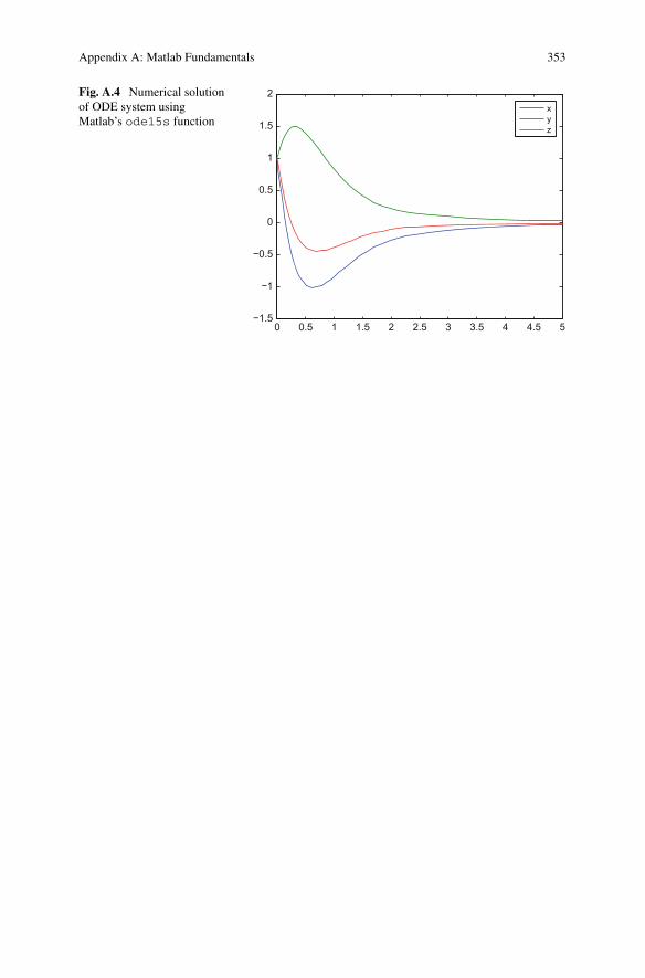
Executing this code produces the plot shown in Fig.A.4. Note that the user-definedderivs function above included botht andx as arguments, even though onlyxwasstrictly required in this example (the time-derivatives of this systemare functions onlyof x). However, ode15s requires the user-specified derivative-evaluation functionto include both t and x as arguments.


Fig. A.4 Numerical solutionof ODE system usingMatlab’s ode15s function

0 0.5 1 1.5 2 2.5 3 3.5 4 4.5 5−1.5

−1

−0.5

0

0.5

1

1.5

2xyz

Appendix BOverview of COMSOL Multiphysics

COMSOL Multiphysics2 is a versatile finite-element software package providing aconvenient means for implementing a wide range of multiphysics models. Theseinclude standard physics modalities such as electromagnetism, structural and fluidmechanics, diffusion and heat transfer, as well as user-defined systems. Its multi-physics coupling capabilities render COMSOL an increasingly popular choice forbioengineering modelling. Optional add-on modules provide user-interfaces andfunctionality for additional physics implementations including electromagnetics,microelectromechanical systems (MEMS), heat transfer, nonlinear structural materi-als, fluid mechanics, microfluidics, as well as interfaces to other software such as theLiveLink for Matlab interface, which allows COMSOL models to be implementedfrom within Matlab.

B.1 COMSOL Basics

COMSOL has undergone several changes to its user-interface since early versionspre-2005. This section provides an overview of COMSOL v5.2, the most recentrelease at the time of writing.

B.1.1 User Interface

The default COMSOL user-interface consists of several windows, as shown inFig.B.1. These include the Model Builder Window, which provides a tree repre-sentation of the current model, the Settings Window which reports associated modelsettingswhen clicking a node in themodel tree, theGraphicsWindow, which displaysthe model geometry, mesh and results, and the Information Windows which provide

2COMSOL Inc., Burlington, MA.


355

356 Appendix B: Overview of COMSOL Multiphysics

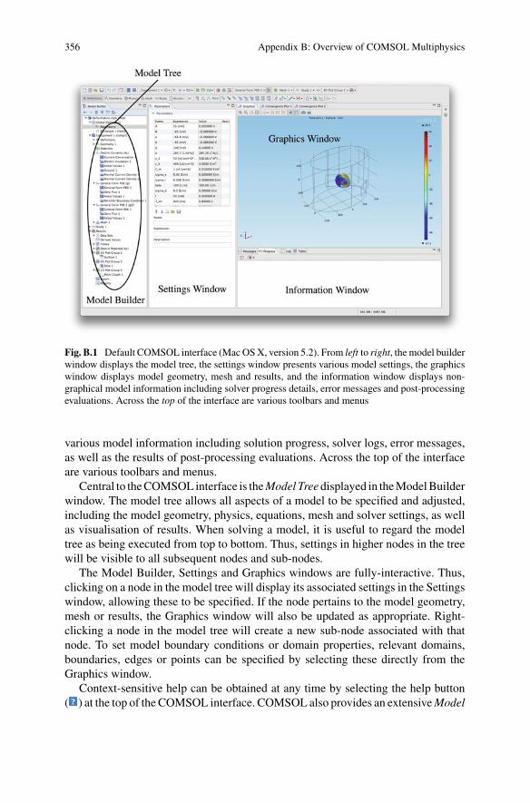
Fig. B.1 Default COMSOL interface (MacOSX, version 5.2). From left to right, themodel builderwindow displays the model tree, the settings window presents various model settings, the graphicswindow displays model geometry, mesh and results, and the information window displays non-graphical model information including solver progress details, error messages and post-processingevaluations. Across the top of the interface are various toolbars and menus

various model information including solution progress, solver logs, error messages,as well as the results of post-processing evaluations. Across the top of the interfaceare various toolbars and menus.

Central to theCOMSOL interface is theModel Treedisplayed in theModelBuilderwindow. The model tree allows all aspects of a model to be specified and adjusted,including the model geometry, physics, equations, mesh and solver settings, as wellas visualisation of results. When solving a model, it is useful to regard the modeltree as being executed from top to bottom. Thus, settings in higher nodes in the treewill be visible to all subsequent nodes and sub-nodes.

The Model Builder, Settings and Graphics windows are fully-interactive. Thus,clicking on a node in the model tree will display its associated settings in the Settingswindow, allowing these to be specified. If the node pertains to the model geometry,mesh or results, the Graphics window will also be updated as appropriate. Right-clicking a node in the model tree will create a new sub-node associated with thatnode. To set model boundary conditions or domain properties, relevant domains,boundaries, edges or points can be specified by selecting these directly from theGraphics window.

Context-sensitive help can be obtained at any time by selecting the help button( ) at the top of the COMSOL interface. COMSOL also provides an extensiveModel

Appendix B: Overview of COMSOL Multiphysics 357

Library containing a range of models with step by step instructions for implementa-tion.

B.1.2 Specifying Models

COMSOL provides a series of tools and interfaces for implementing models fromscratch, including the Model Wizard, geometry tools, physics and user-equationinterfaces, mesh and solver settings, parameters, variables and model couplings, aswell as post-processing analysis and visualisation.

B.1.2.1 The Model Wizard

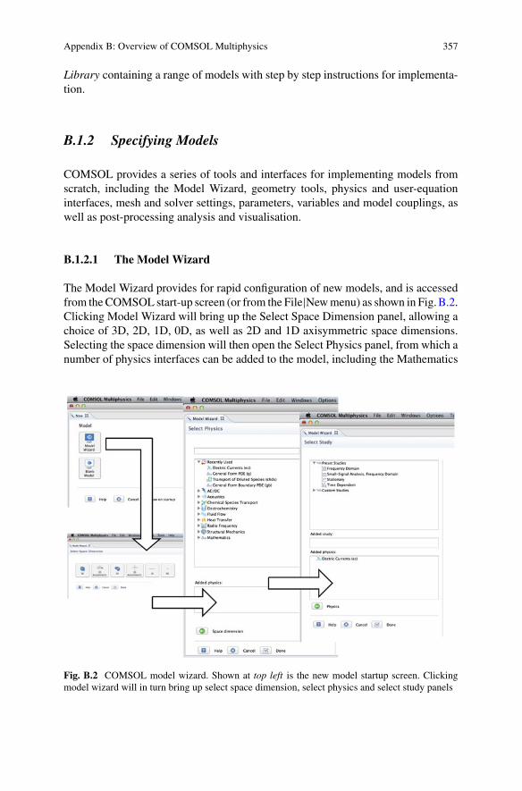
The Model Wizard provides for rapid configuration of new models, and is accessedfrom theCOMSOL start-up screen (or from the File|Newmenu) as shown in Fig.B.2.Clicking Model Wizard will bring up the Select Space Dimension panel, allowing achoice of 3D, 2D, 1D, 0D, as well as 2D and 1D axisymmetric space dimensions.Selecting the space dimension will then open the Select Physics panel, from which anumber of physics interfaces can be added to the model, including the Mathematics

Fig. B.2 COMSOL model wizard. Shown at top left is the new model startup screen. Clickingmodel wizard will in turn bring up select space dimension, select physics and select study panels


interface for specifying user-defined equations. The list of physics interfaces dis-played will depend on which optional COMSOLmodules have been installed. Inter-faces can be added to the model by clicking the “Add” button. Additional physicsinterfaces can also be added later from the model tree.

Once the required physics interfaces have been added, clicking the Study forwardarrow button ( ) will open the Select Study panel for specifying a default study(i.e. solver) for the model. Depending on the physics interface(s) selected, the choiceof solver can include Stationary, Time Dependent or Frequency Domain. Additionalstudies can also be added later to the same model. Clicking “Done” will exit theModel Wizard and display the main COMSOL interface with model tree configuredaccording to the specified Model Wizard settings.

B.1.2.2 Creating a Geometry

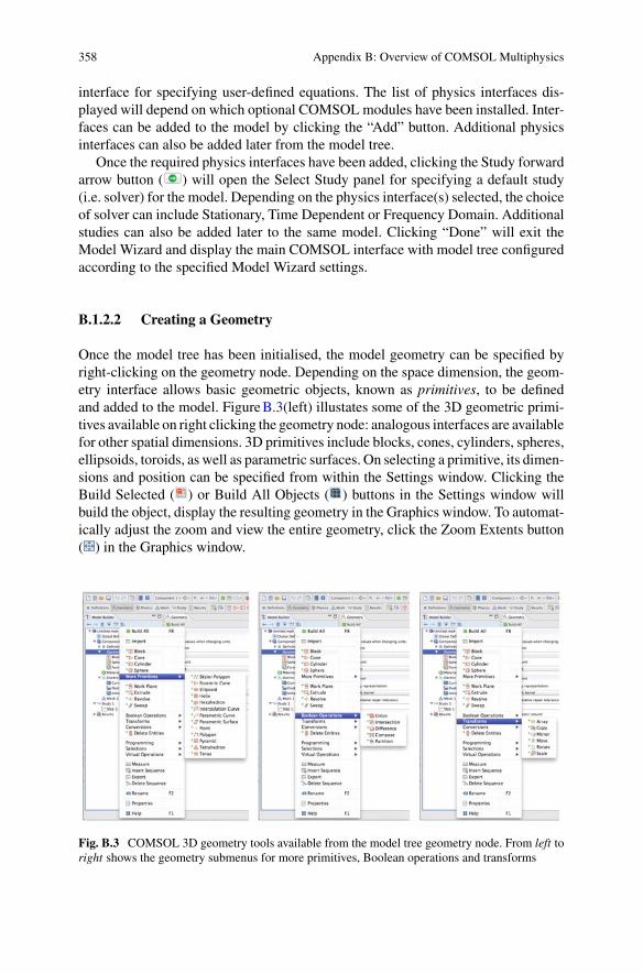
Once the model tree has been initialised, the model geometry can be specified byright-clicking on the geometry node. Depending on the space dimension, the geom-etry interface allows basic geometric objects, known as primitives, to be definedand added to the model. FigureB.3(left) illustates some of the 3D geometric primi-tives available on right clicking the geometry node: analogous interfaces are availablefor other spatial dimensions. 3D primitives include blocks, cones, cylinders, spheres,ellipsoids, toroids, as well as parametric surfaces. On selecting a primitive, its dimen-sions and position can be specified from within the Settings window. Clicking theBuild Selected ( ) or Build All Objects ( ) buttons in the Settings window willbuild the object, display the resulting geometry in the Graphics window. To automat-ically adjust the zoom and view the entire geometry, click the Zoom Extents button( ) in the Graphics window.

Fig. B.3 COMSOL 3D geometry tools available from the model tree geometry node. From left toright shows the geometry submenus for more primitives, Boolean operations and transforms


By right-clicking the geometry node, it is also possible to perform Boolean opera-tions on geometric primitives, including subtracting objects from each other, formingunions and intersections, as well as custom combinations of these (Fig.B.3, middle).It is also possible to transform objects by moving, scaling, rotating, mirroring orcopying (Fig.B.3, right). Geometric objects for Boolean operations and transforma-tions can be selected using the Graphics window.

In 3D, it is also possible to define aWork Plane, a 2D plane embedded in the 3Dgeometry, again by right-clicking the geometry node. 2D primitives can be specifiedby right-clicking the associated plane geometry sub-node. These 2D objects can thenbe revolved or extruded into the 3D geometry.

Using a combination of COMSOL’s in-built geometry tools, it is possible to con-struct fairly complex objects and shapes. For specifying more complex geometries,it is also possible to import CAD, STL and VRML files.

All geometric primitives, operations and transforms appear as geometry sub-nodesin the model tree. It is possible to click on an existing node in any order and modifyits settings. Clicking the “Build All Objects” button in the Settings window will thenupdate the geometry.

B.1.2.3 User-Defined Parameters, Functions and Variables

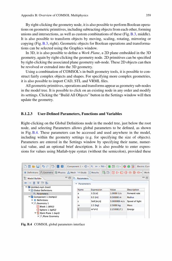
Right-clicking on the Global Definitions node in the model tree, just below the rootnode, and selecting Parameters allows global parameters to be defined, as shownin Fig.B.4. These parameters can be accessed and used anywhere in the model,including within the geometry settings (e.g. for specifying the size of objects).Parameters are entered in the Settings window by specifying their name, numer-ical value, and an optional brief description. It is also possible to enter expres-sions for values using Matlab-type syntax (without the semicolon), provided these

Fig. B.4 COMSOL global parameters interface


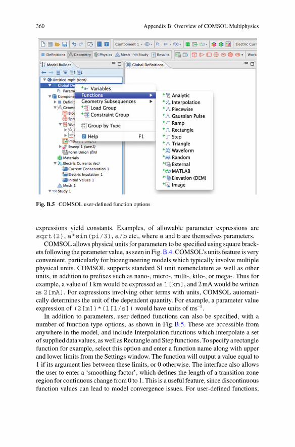
Fig. B.5 COMSOL user-defined function options

expressions yield constants. Examples, of allowable parameter expressions aresqrt(2), a*sin(pi/3), a/b etc., where a and b are themselves parameters.

COMSOL allows physical units for parameters to be specified using square brack-ets following the parameter value, as seen in Fig.B.4. COMSOL’s units feature is veryconvenient, particularly for bioengineering models which typically involve multiplephysical units. COMSOL supports standard SI unit nomenclature as well as otherunits, in addition to prefixes such as nano-, micro-, milli-, kilo-, or mega-. Thus forexample, a value of 1km would be expressed as 1[km], and 2mA would be writtenas 2[mA]. For expressions involving other terms with units, COMSOL automati-cally determines the unit of the dependent quantity. For example, a parameter valueexpression of (2[m])*(1[1/s]) would have units of ms–1.

In addition to parameters, user-defined functions can also be specified, with anumber of function type options, as shown in Fig.B.5. These are accessible fromanywhere in the model, and include Interpolation functions which interpolate a setof supplied data values, aswell asRectangle andStep functions. To specify a rectanglefunction for example, select this option and enter a function name along with upperand lower limits from the Settings window. The function will output a value equal to1 if its argument lies between these limits, or 0 otherwise. The interface also allowsthe user to enter a ‘smoothing factor’, which defines the length of a transition zoneregion for continuous change from 0 to 1. This is a useful feature, since discontinuousfunction values can lead to model convergence issues. For user-defined functions,


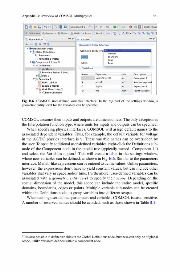
Fig. B.6 COMSOL user-defined variables interface. In the top part of the settings window, ageometric entity level for the variables can be specified

COMSOL assumes their inputs and outputs are dimensionless. The only exception isthe Interpolation function type, where units for inputs and outputs can be specified.

When specifying physics interfaces, COMSOL will assign default names to theassociated dependent variables. Thus, for example, the default variable for voltagein the AC/DC physics interface is V. These variable names can be overridden bythe user. To specify additional user-defined variables, right-click the Definitions sub-node of the Component node in the model tree (typically named “Component 1”)and select the Variables option.3 This will create a table in the settings window,where new variables can be defined, as shown in Fig.B.6. Similar to the parametersinterface,Matlab-like expressions can be entered to define values. Unlike parameters,however, the expressions don’t have to yield constant values, but can include othervariables that vary in space and/or time. Furthermore, user-defined variables can beassociated with a geometric entity level to specify their scope. Depending on thespatial dimension of the model, this scope can include the entire model, specificdomains, boundaries, edges or points. Multiple variable sub-nodes can be createdwithin the Definitions node, to group variables into different scopes.

When naming user-defined parameters and variables, COMSOL is case-sensitive.A number of reserved names should be avoided, such as those shown in TableB.1.

3It is also possible to define variables in the Global Definitions node, but these can only be of globalscope, unlike variables defined within a component node.


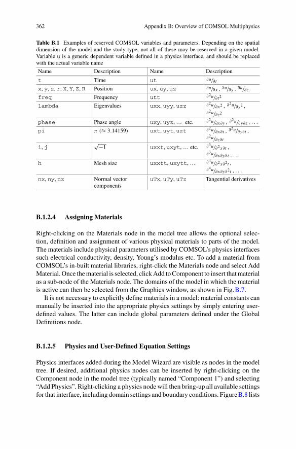
Table B.1 Examples of reserved COMSOL variables and parameters. Depending on the spatialdimension of the model and the study type, not all of these may be reserved in a given model.Variable u is a generic dependent variable defined in a physics interface, and should be replacedwith the actual variable name

Name Description Name Description

t Time ut ∂u/∂t

x, y, z, r, X, Y, Z, R Position ux, uy, uz ∂u/∂x , ∂u/∂y , ∂u/∂z

freq Frequency utt ∂2u/∂t2

lambda Eigenvalues uxx, uyy, uzz ∂2u/∂x2 , ∂2u/∂y2 ,∂2u/∂z2

phase Phase angle uxy, uyz, … etc. ∂2u/∂x∂y , ∂2u/∂y∂z , . . .

pi π (≈ 3.14159) uxt, uyt, uzt ∂2u/∂x∂t , ∂2u/∂y∂t ,∂2u/∂z∂t

i, j√−1 uxxt, uxyt, … etc. ∂3u/∂2x∂t ,

∂3u/∂x∂y∂t , . . .

h Mesh size uxxtt, uxytt, … ∂4u/∂2x∂2t ,∂4u/∂x∂y∂2t , . . .

nx, ny, nz Normal vectorcomponents

uTx, uTy, uTz Tangential derivatives

B.1.2.4 Assigning Materials

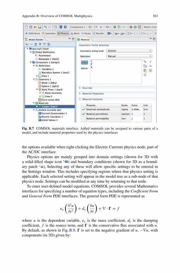
Right-clicking on the Materials node in the model tree allows the optional selec-tion, definition and assignment of various physical materials to parts of the model.The materials include physical parameters utilised by COMSOL’s physics interfacessuch electrical conductivity, density, Young’s modulus etc. To add a material fromCOMSOL’s in-built material libraries, right-click the Materials node and select AddMaterial. Once thematerial is selected, clickAdd toComponent to insert thatmaterialas a sub-node of the Materials node. The domains of the model in which the materialis active can then be selected from the Graphics window, as shown in Fig.B.7.

It is not necessary to explicitly define materials in a model: material constants canmanually be inserted into the appropriate physics settings by simply entering user-defined values. The latter can include global parameters defined under the GlobalDefinitions node.

B.1.2.5 Physics and User-Defined Equation Settings

Physics interfaces added during the Model Wizard are visible as nodes in the modeltree. If desired, additional physics nodes can be inserted by right-clicking on theComponent node in the model tree (typically named “Component 1”) and selecting“Add Physics”. Right-clicking a physics node will then bring-up all available settingsfor that interface, including domain settings and boundary conditions. FigureB.8 lists


Fig. B.7 COMSOL materials interface. Added materials can be assigned to various parts of amodel, and include material properties used by the physics interfaces

the options available when right-clicking the Electric Currents physics node, part ofthe AC/DC interface.

Physics options are mainly grouped into domain settings (shown for 3D witha solid-filled shape icon ) and boundary conditions (shown for 3D as a bound-ary patch ). Selecting any of these will allow specific settings to be entered inthe Settings window. This includes specifying regions where that physics setting isapplicable. Each selected setting will appear in the model tree as a sub-node of thatphysics node. Settings can be modified at any time by returning to that node.

To enter user-defined model equations, COMSOL provides several Mathematicsinterfaces for specifying a number of equation types, including the Coefficient Formand General Form PDE interfaces. The general form PDE is represented as

ea

(∂2u

∂t2

)+ da

(∂u

∂t

)+ ∇ · � = f

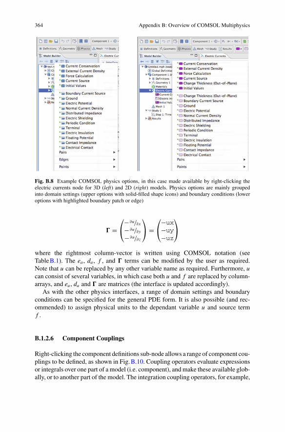
where u is the dependent variable, ea is the mass coefficient, da is the dampingcoefficient, f is the source term, and � is the conservative flux associated with u.By default, as shown in Fig.B.9, � is set to the negative gradient of u, −∇u, withcomponents (in 3D) given by:


Fig. B.8 Example COMSOL physics options, in this case made available by right-clicking theelectric currents node for 3D (left) and 2D (right) models. Physics options are mainly groupedinto domain settings (upper options with solid-filled shape icons) and boundary conditions (loweroptions with highlighted boundary patch or edge)

� =⎛⎝−∂u/∂x

−∂u/∂y−∂u/∂z

⎞⎠ =

⎛⎝−ux

−uy−uz

⎞⎠

where the rightmost column-vector is written using COMSOL notation (seeTableB.1). The ea , da , f , and � terms can be modified by the user as required.Note that u can be replaced by any other variable name as required. Furthermore, ucan consist of several variables, in which case both u and f are replaced by column-arrays, and ea , da and � are matrices (the interface is updated accordingly).

As with the other physics interfaces, a range of domain settings and boundaryconditions can be specified for the general PDE form. It is also possible (and rec-ommended) to assign physical units to the dependant variable u and source termf .

B.1.2.6 Component Couplings

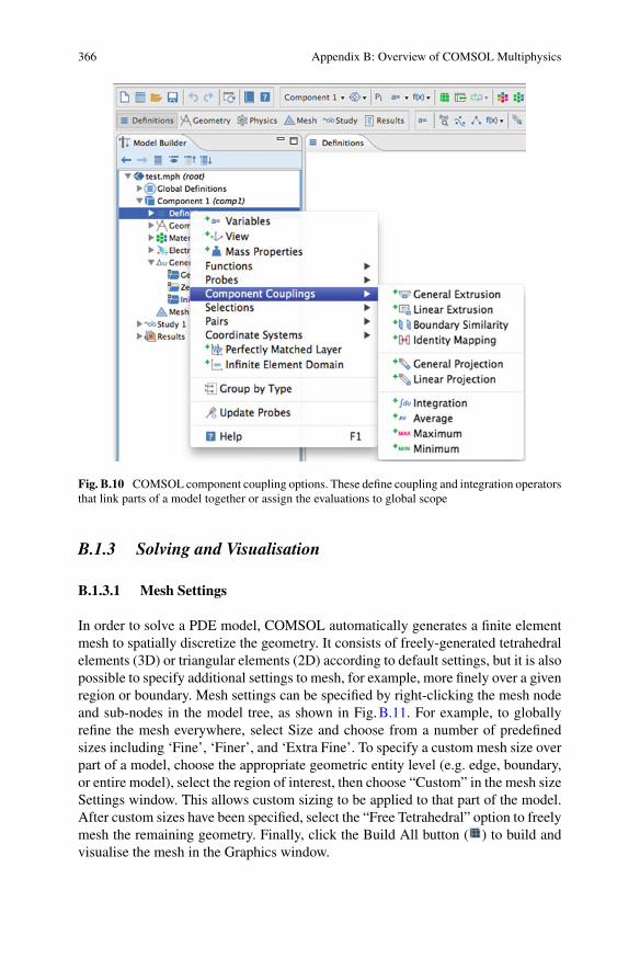
Right-clicking the component definitions sub-node allows a range of component cou-plings to be defined, as shown in Fig.B.10. Coupling operators evaluate expressionsor integrals over one part of a model (i.e. component), andmake these available glob-ally, or to another part of the model. The integration coupling operators, for example,


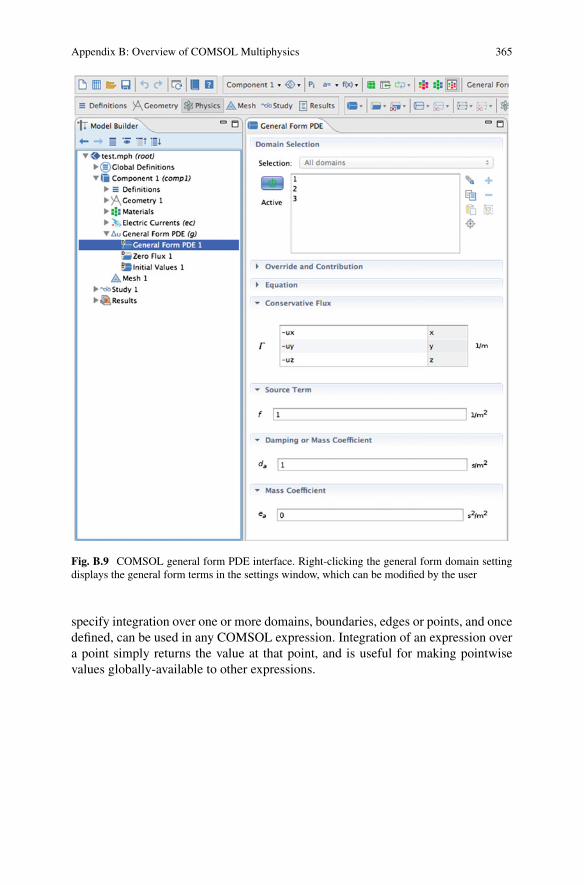
Fig. B.9 COMSOL general form PDE interface. Right-clicking the general form domain settingdisplays the general form terms in the settings window, which can be modified by the user

specify integration over one or more domains, boundaries, edges or points, and oncedefined, can be used in any COMSOL expression. Integration of an expression overa point simply returns the value at that point, and is useful for making pointwisevalues globally-available to other expressions.


Fig. B.10 COMSOL component coupling options. These define coupling and integration operatorsthat link parts of a model together or assign the evaluations to global scope

B.1.3 Solving and Visualisation

B.1.3.1 Mesh Settings

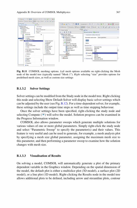
In order to solve a PDE model, COMSOL automatically generates a finite elementmesh to spatially discretize the geometry. It consists of freely-generated tetrahedralelements (3D) or triangular elements (2D) according to default settings, but it is alsopossible to specify additional settings to mesh, for example, more finely over a givenregion or boundary. Mesh settings can be specified by right-clicking the mesh nodeand sub-nodes in the model tree, as shown in Fig.B.11. For example, to globallyrefine the mesh everywhere, select Size and choose from a number of predefinedsizes including ‘Fine’, ‘Finer’, and ‘Extra Fine’. To specify a custom mesh size overpart of a model, choose the appropriate geometric entity level (e.g. edge, boundary,or entire model), select the region of interest, then choose “Custom” in the mesh sizeSettings window. This allows custom sizing to be applied to that part of the model.After custom sizes have been specified, select the “Free Tetrahedral” option to freelymesh the remaining geometry. Finally, click the Build All button ( ) to build andvisualise the mesh in the Graphics window.


Fig. B.11 COMSOL meshing options. Left mesh options available on right-clicking the Meshnode of the model tree (typically named “Mesh 1”). Right selecting “size” provides options forpredefined mesh sizes, as well as custom size settings

B.1.3.2 Solver Settings

Solver settings can be modified from the Study node in the model tree. Right clickingthis node and selecting Show Default Solver will display basic solver settings whichcan be adjusted by the user (see Fig.B.12). For a time-dependent solver, for example,these settings include the output time steps as well as time stepping behaviour.

Once the solver settings have been specified, right-clicking the study node andselecting Compute ( ) will solve the model. Solution progress can be examined inthe Progress Information window.

COMSOL also allows parameter sweeps which generate multiple solutions forvarious values of one or more global parameters. Simply right-click the study nodeand select “Parametric Sweep” to specify the parameter(s) and their values. Thisfeature is very useful and can be used to generate, for example, a mesh analysis plotby specifying a mesh size global parameter, assigning the maximum mesh size tothis parameter, and then performing a parameter sweep to examine how the solutionchanges with mesh size.

B.1.3.3 Visualisation of Results

On solving a model, COMSOL will automatically generate a plot of the primarydependent variable in the Graphics window. Depending on the spatial dimension ofthe model, the default plot is either a multislice plot (3D model), a surface plot (2Dmodel), or a line plot (1D model). Right-clicking the Results node in the model treeallows additional plots to be defined, including arrow and streamline plots, contour


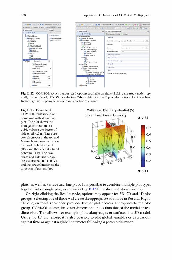
Fig. B.12 COMSOL solver options. Left options available on right-clicking the study node (typ-ically named “study 1”). Right selecting “show default solver” provides options for the solver.Including time stepping behaviour and absolute tolerance

Fig. B.13 Example ofCOMSOL multislice plotcombined with streamlineplot. The plot shows thevoltage distribution in acubic volume conductor ofsidelength 0.5m. There aretwo electrodes at the top andbottom boundaries, with oneelectrode held at ground(0V) and the other at a fixedpotential (1V). The twoslices and colourbar showthe electric potential (in V),and the streamlines show thedirection of current flow

plots, as well as surface and line plots. It is possible to combine multiple plot typestogether into a single plot, as shown in Fig.B.13 for a slice and streamline plot.

On right-clicking the Results node, options may appear for 3D, 2D and 1D plotgroups. Selecting one of these will create the appropriate sub-node in Results. Right-clicking on these sub-nodes provides further plot choices appropriate to the plotgroup. COMSOL allows for lower-dimensional plots than that of the model space-dimension. This allows, for example, plots along edges or surfaces in a 3D model.Using the 1D plot group, it is also possible to plot global variables or expressionsagainst time or against a global parameter following a parametric sweep.


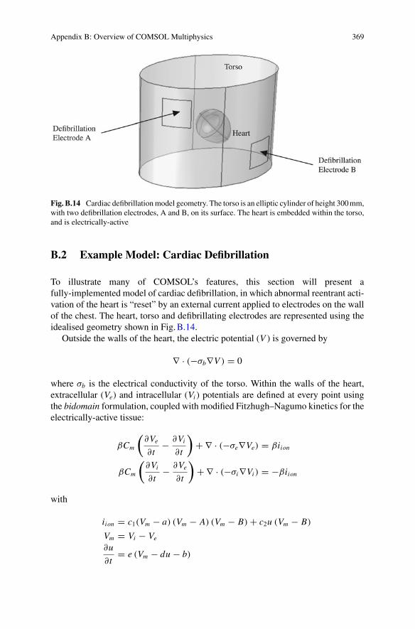
Fig. B.14 Cardiac defibrillationmodel geometry. The torso is an elliptic cylinder of height 300mm,with two defibrillation electrodes, A and B, on its surface. The heart is embedded within the torso,and is electrically-active

B.2 Example Model: Cardiac Defibrillation

To illustrate many of COMSOL’s features, this section will present afully-implemented model of cardiac defibrillation, in which abnormal reentrant acti-vation of the heart is “reset” by an external current applied to electrodes on the wallof the chest. The heart, torso and defibrillating electrodes are represented using theidealised geometry shown in Fig.B.14.

Outside the walls of the heart, the electric potential (V ) is governed by

∇ · (−σb∇V ) = 0

where σb is the electrical conductivity of the torso. Within the walls of the heart,extracellular (Ve) and intracellular (Vi ) potentials are defined at every point usingthe bidomain formulation, coupled with modified Fitzhugh–Nagumo kinetics for theelectrically-active tissue:

βCm

(∂Ve

∂t− ∂Vi

∂t

)+ ∇ · (−σe∇Ve) = βiion

βCm

(∂Vi

∂t− ∂Ve

∂t

)+ ∇ · (−σi∇Vi ) = −βiion

with

iion = c1(Vm − a) (Vm − A) (Vm − B) + c2u (Vm − B)

Vm = Vi − Ve

∂u

∂t= e (Vm − du − b)


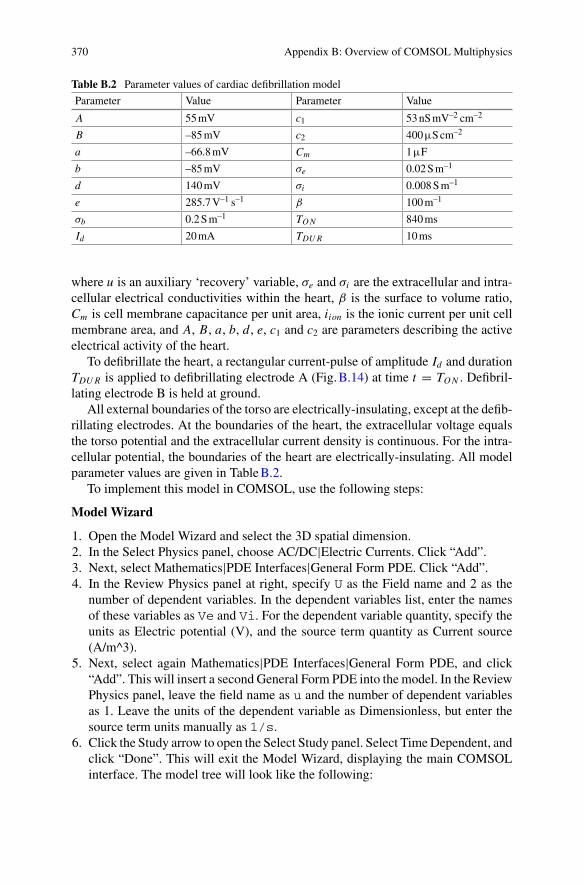
Table B.2 Parameter values of cardiac defibrillation model

Parameter Value Parameter Value

A 55mV c1 53nSmV–2 cm–2

B –85mV c2 400μScm–2

a –66.8mV Cm 1μF

b –85mV σe 0.02Sm–1

d 140mV σi 0.008Sm–1

e 285.7V–1 s–1 β 100m–1

σb 0.2Sm–1 TON 840ms

Id 20mA TDUR 10ms

where u is an auxiliary ‘recovery’ variable, σe and σi are the extracellular and intra-cellular electrical conductivities within the heart, β is the surface to volume ratio,Cm is cell membrane capacitance per unit area, iion is the ionic current per unit cellmembrane area, and A, B, a, b, d, e, c1 and c2 are parameters describing the activeelectrical activity of the heart.

To defibrillate the heart, a rectangular current-pulse of amplitude Id and durationTDUR is applied to defibrillating electrode A (Fig.B.14) at time t = TON . Defibril-lating electrode B is held at ground.

All external boundaries of the torso are electrically-insulating, except at the defib-rillating electrodes. At the boundaries of the heart, the extracellular voltage equalsthe torso potential and the extracellular current density is continuous. For the intra-cellular potential, the boundaries of the heart are electrically-insulating. All modelparameter values are given in TableB.2.

To implement this model in COMSOL, use the following steps:

Model Wizard

1. Open the Model Wizard and select the 3D spatial dimension.2. In the Select Physics panel, choose AC/DC|Electric Currents. Click “Add”.3. Next, select Mathematics|PDE Interfaces|General Form PDE. Click “Add”.4. In the Review Physics panel at right, specify U as the Field name and 2 as the

number of dependent variables. In the dependent variables list, enter the namesof these variables as Ve and Vi. For the dependent variable quantity, specify theunits as Electric potential (V), and the source term quantity as Current source(A/m^3).

5. Next, select again Mathematics|PDE Interfaces|General Form PDE, and click“Add”. This will insert a second General Form PDE into the model. In the ReviewPhysics panel, leave the field name as u and the number of dependent variablesas 1. Leave the units of the dependent variable as Dimensionless, but enter thesource term units manually as 1/s.

6. Click the Study arrow to open the Select Study panel. Select TimeDependent, andclick “Done”. This will exit the Model Wizard, displaying the main COMSOLinterface. The model tree will look like the following:


Geometry

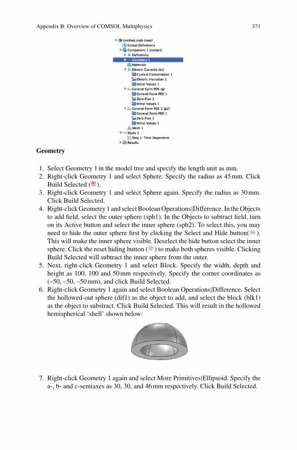
1. Select Geometry 1 in the model tree and specify the length unit as mm.2. Right-click Geometry 1 and select Sphere. Specify the radius as 45mm. Click

Build Selected ( ).3. Right-click Geometry 1 and select Sphere again. Specify the radius as 30mm.

Click Build Selected.4. Right-clickGeometry 1 and selectBooleanOperations|Difference. In theObjects

to add field, select the outer sphere (sph1). In the Objects to subtract field, turnon its Active button and select the inner sphere (sph2). To select this, you mayneed to hide the outer sphere first by clicking the Select and Hide button( ).This will make the inner sphere visible. Deselect the hide button select the innersphere. Click the reset hiding button ( ) to make both spheres visible. ClickingBuild Selected will subtract the inner sphere from the outer.

5. Next, right-click Geometry 1 and select Block. Specify the width, depth andheight as 100, 100 and 50mm respectively. Specify the corner coordinates as(–50, –50, –50mm), and click Build Selected.

6. Right-click Geometry 1 again and select Boolean Operations|Difference. Selectthe hollowed-out sphere (dif1) as the object to add, and select the block (blk1)as the object to substract. Click Build Selected. This will result in the hollowedhemispherical ‘shell’ shown below:

7. Right-click Geometry 1 again and select More Primitives|Ellipsoid. Specify thea-, b- and c-semiaxes as 30, 30, and 46mm respectively. Click Build Selected.


8. Right-click Geometry 1, selecting again More Primitives|Ellipsoid. This time,specify the a-, b- and c-semiaxes as 45, 45, and 69mm respectively. Click BuildSelected.

9. Right-click Geometry 1 and select Block. Specify the width, depth and height toall be 100mm. Specify the corner of the block to be at (–50, –50, 0mm). ClickBuild Selected.

10. Right-click Geometry 1 again and select Boolean Operations|Difference. Selectthe outer ellipsoid (elp1) as the object to add, and select the block (blk2) as theobject to substract. Click Build Selected.

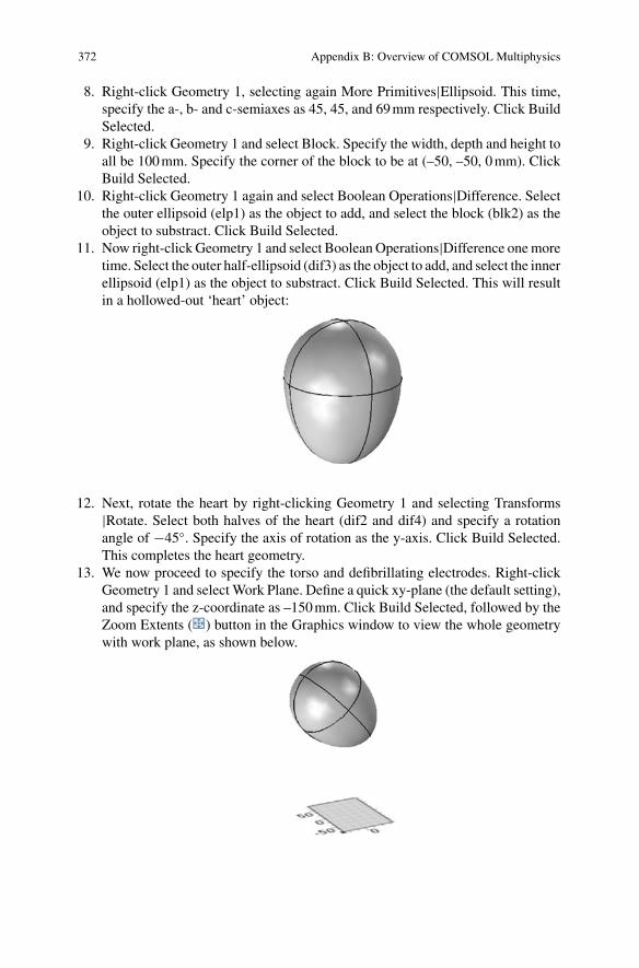
11. Now right-click Geometry 1 and select BooleanOperations|Difference onemoretime. Select the outer half-ellipsoid (dif3) as the object to add, and select the innerellipsoid (elp1) as the object to substract. Click Build Selected. This will resultin a hollowed-out ‘heart’ object:

12. Next, rotate the heart by right-clicking Geometry 1 and selecting Transforms|Rotate. Select both halves of the heart (dif2 and dif4) and specify a rotationangle of −45◦. Specify the axis of rotation as the y-axis. Click Build Selected.This completes the heart geometry.

13. We now proceed to specify the torso and defibrillating electrodes. Right-clickGeometry 1 and select Work Plane. Define a quick xy-plane (the default setting),and specify the z-coordinate as –150mm. Click Build Selected, followed by theZoom Extents ( ) button in the Graphics window to view the whole geometrywith work plane, as shown below.


14. Now, right-click on the Plane Geometry subnode of Work Plane 1 and selectEllipse. Specify the a- and b-semiaxes as 200 and 125mm respectively. Specifythe (xw, yw) position of the centre to be (0, 30mm) and click Build Selected.Click the Zoom Extents ( ) button to see the whole ellipse.

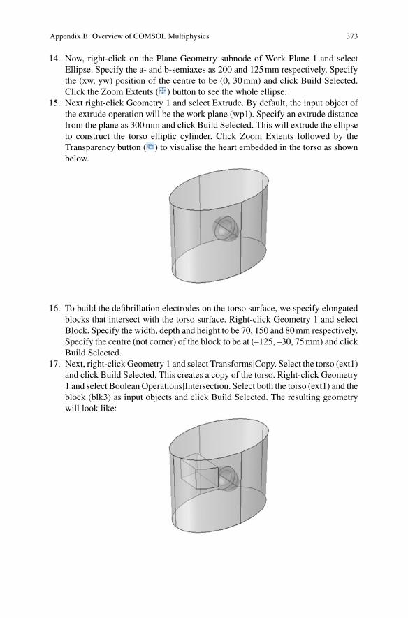
15. Next right-click Geometry 1 and select Extrude. By default, the input object ofthe extrude operation will be the work plane (wp1). Specify an extrude distancefrom the plane as 300mm and click Build Selected. This will extrude the ellipseto construct the torso elliptic cylinder. Click Zoom Extents followed by theTransparency button ( ) to visualise the heart embedded in the torso as shownbelow.

16. To build the defibrillation electrodes on the torso surface, we specify elongatedblocks that intersect with the torso surface. Right-click Geometry 1 and selectBlock. Specify the width, depth and height to be 70, 150 and 80mm respectively.Specify the centre (not corner) of the block to be at (–125, –30, 75mm) and clickBuild Selected.

17. Next, right-click Geometry 1 and select Transforms|Copy. Select the torso (ext1)and click Build Selected. This creates a copy of the torso. Right-click Geometry1 and select Boolean Operations|Intersection. Select both the torso (ext1) and theblock (blk3) as input objects and click Build Selected. The resulting geometrywill look like:


18. Now we repeat this procedure for the other electrode. Right-click Geometry 1and select Block. Specify the width, depth and height to be 70, 150 and 80mmrespectively. Specify the centre of the block to now be at (125, –30, –75mm)and click Build Selected.

19. As before, right-click Geometry 1 and select Transforms|Copy. Select the torso(copy1) and click Build Selected. Right-click Geometry 1 and select BooleanOperations|Intersection. Select both the torso (copy1) and the block (blk4) asinput objects and click Build Selected.

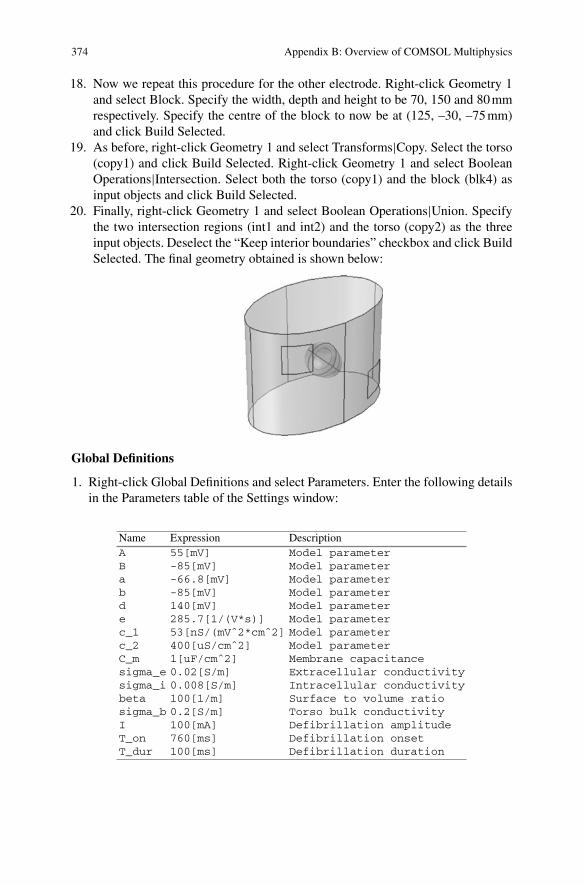
20. Finally, right-click Geometry 1 and select Boolean Operations|Union. Specifythe two intersection regions (int1 and int2) and the torso (copy2) as the threeinput objects. Deselect the “Keep interior boundaries” checkbox and click BuildSelected. The final geometry obtained is shown below:

Global Definitions

1. Right-click Global Definitions and select Parameters. Enter the following detailsin the Parameters table of the Settings window:

Name Expression DescriptionA 55[mV] Model parameterB -85[mV] Model parametera -66.8[mV] Model parameterb -85[mV] Model parameterd 140[mV] Model parametere 285.7[1/(V*s)] Model parameterc_1 53[nS/(mVˆ2*cmˆ2] Model parameterc_2 400[uS/cmˆ2] Model parameterC_m 1[uF/cmˆ2] Membrane capacitancesigma_e 0.02[S/m] Extracellular conductivitysigma_i 0.008[S/m] Intracellular conductivitybeta 100[1/m] Surface to volume ratiosigma_b 0.2[S/m] Torso bulk conductivityI 100[mA] Defibrillation amplitudeT_on 760[ms] Defibrillation onsetT_dur 100[ms] Defibrillation duration


2. Right-click Global Definitions and select Functions|Rectangle. Specify the lowerlimit asT_on and the upper limit asT_on+T_dur. In the Smoothing tab, specifythe size of the transition zone asT_dur/10. Leave the functionname to its default(rect1).

Component Definitions

1. Right-click the Definitions sub-node of Component 1 and select ComponentCouplings|Integration. Specify the geometric entity level as ‘Boundary’ and selectboundary 5. This creates an integration operator for integrating expressions overthis boundary. Leave the default operator name as intop1.

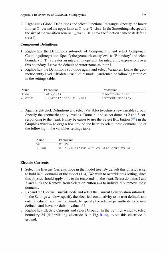
2. Right-click the Definitions sub-node again and select Variables. Leave the geo-metric entity level to its default as ‘Entiremodel’, and enter the following variablesin the settings table:

Name Expression DescriptionArea intop1(1) Electrode areaJ_stim (I/Area)*rect1(t[1/s]) Current density

3. Again, right-clickDefinitions and select Variables to define a newvariables group.Specify the geometric entity level as ‘Domain’ and select domains 2 and 3 cor-responding to the heart. It may be easier to use the Select Box button ( ) in theGraphics window to drag a box around the heart to select these domains. Enterthe following in the variables settings table:

Name ExpressionVm Vi-Vei_ion c_1*(Vm-a)*(Vm-A)*(Vm-B)+c_2*u*(Vm-B)

Electric Currents

1. Select the Electric Currents node in the model tree. By default this physics is setto hold in all domains of the model (1–4). We wish to override this setting, sincethis physics should apply only to the torso and not the heart. Select domains 2 and3 and click the Remove from Selection button ( ) to individually remove thesedomains.

2. Expand the Electric Currents node and select the Current Conservation sub-node.In the Settings window, specify the electrical conductivity to be user defined, andenter a value of sigma_b. Similarly, specify the relative permittivity to be userdefined, and leave the default value of 1.

3. Right-click Electric Currents and select Ground. In the Settings window, selectboundary 25 (defibrillating electrode B in Fig.B.14), to set this electrode toground.


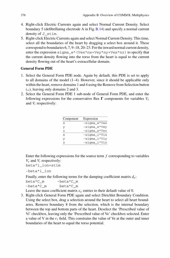
4. Right-click Electric Currents again and select Normal Current Density. Selectboundary 5 (defibrillating electrode A in Fig.B.14) and specify a normal currentdensity of J_stim.

5. Right-click Electric Currents again and select Normal Current Density. This time,select all the boundaries of the heart by dragging a select box around it. Thesecorrespond to boundaries 6, 7, 9–18, 20–23. For the inward normal current density,enter the expression sigma_e*(Vex*nx+Vey*ny+Vex*nz) to specify thatthe current density flowing into the torso from the heart is equal to the currentdensity flowing out of the heart’s extracellular domain.

General Form PDE

1. Select the General Form PDE node. Again by default, this PDE is set to applyto all domains of the model (1–4). However, since it should be applicable onlywithin the heart, remove domains 1 and 4 using the Remove fromSelection button( ), leaving only domains 2 and 3.

2. Select the General Form PDE 1 sub-node of General Form PDE, and enter thefollowing expressions for the conservative flux � components for variables Ve

and Vi respectively:

Component Expressionx -sigma_e*Vexy -sigma_e*Veyz -sigma_e*Vezx -sigma_i*Vixy -sigma_i*Viyz -sigma_i*Viz

Enter the following expressions for the source term f corresponding to variablesVe and Vi respectively:beta*i_ion+stim

-beta*i_ion

Finally, enter the following terms for the damping coefficient matrix da :beta*C_m -beta*C_m-beta*C_m beta*C_mLeave the mass coefficient matrix ea entries to their default value of 0.

3. Right-click General Form PDE again and select Dirichlet Boundary Condition.Using the select box, drag a selection around the heart to select all heart bound-aries. Remove boundary 8 from the selection, which is the internal boundarybetween the top and bottom parts of the heart. Deselect the ‘Prescribed value ofVi’ checkbox, leaving only the ‘Prescribed value of Ve’ checkbox selected. Entera value of V in the r1 field. This constrains the value of Ve at the outer and innerboundaries of the heart to equal the torso potential.


4. Finally, select the Initial Values 1 sub-node of the General Form PDE node.Leave the initial value of Ve to its default value of 0. For Vi however, enterthe initial value expression -0.085 + 0.12*(y<0)*(z>0.02). This setsVi to an initial value of −0.085 + 0.12 = 0.035V for the sector of the heartcorresponding to y < 0 and z > 0.02m, representing an electrically-excitedstate. In all other heart regions, Vi is initially set to –0.085V, corresponding tothe resting, non-excited state.

General Form PDE 2

1. Select the General Form PDE 2 node. Select domains 1 and 4 and individuallyremove these using the Remove from Selection button ( ), leaving only domains2 and 3.

2. Select the General Form PDE 1 sub-node of General Form PDE 2, and enter avalue of 0 for each of the three components of conservative flux �, since thereare no spatial derivatives in the equation for u. For the source term f , enter theexpression e*(Vm-d*u-b) and for the damping and mass coefficients da andea , leave their value as 1 and 0 respectively.

3. Finally, select the Initial Values 1 sub-node of the General Form PDE 2 node, andenter the initial value expression 5*(x>0.03). This sets variable u to an initialvalue of 5 when x > 0.03m, corresponding to heart state that is temporarilyinexcitable (i.e. refractory), and 0 elsewhere.

Mesh

1. Right-click Mesh 1 and select Size. In the Settings window, specify ‘Domain’ asthe geometric entity level, and select domains 2 and 3 corresponding to the heart.Under the Predefined Element Size option, select ‘Finer’ from the dropdown list.

2. Right-clickMesh 1 again and select Free Tetrahedral. Leave the default geometricentity level as ‘Remaining’. This will mesh the remaining parts of the model witha free tetrahedral mesh.

3. Click Build All ( ) in the Settings window to build and display the mesh.

Study

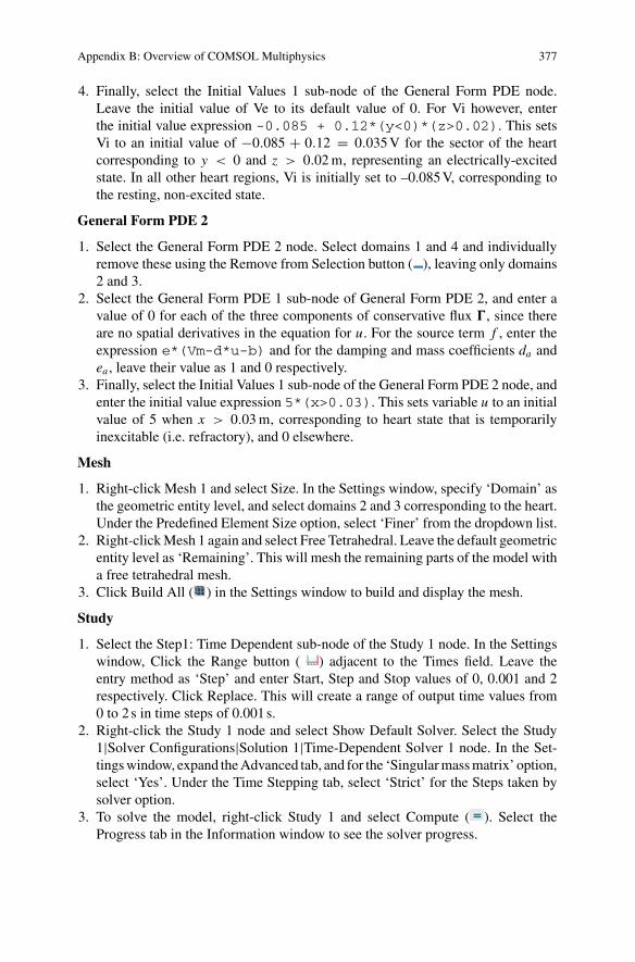
1. Select the Step1: Time Dependent sub-node of the Study 1 node. In the Settingswindow, Click the Range button ( ) adjacent to the Times field. Leave theentry method as ‘Step’ and enter Start, Step and Stop values of 0, 0.001 and 2respectively. Click Replace. This will create a range of output time values from0 to 2s in time steps of 0.001s.

2. Right-click the Study 1 node and select Show Default Solver. Select the Study1|Solver Configurations|Solution 1|Time-Dependent Solver 1 node. In the Set-tingswindow, expand theAdvanced tab, and for the ‘Singularmassmatrix’ option,select ‘Yes’. Under the Time Stepping tab, select ‘Strict’ for the Steps taken bysolver option.

3. To solve the model, right-click Study 1 and select Compute ( ). Select theProgress tab in the Information window to see the solver progress.


Results

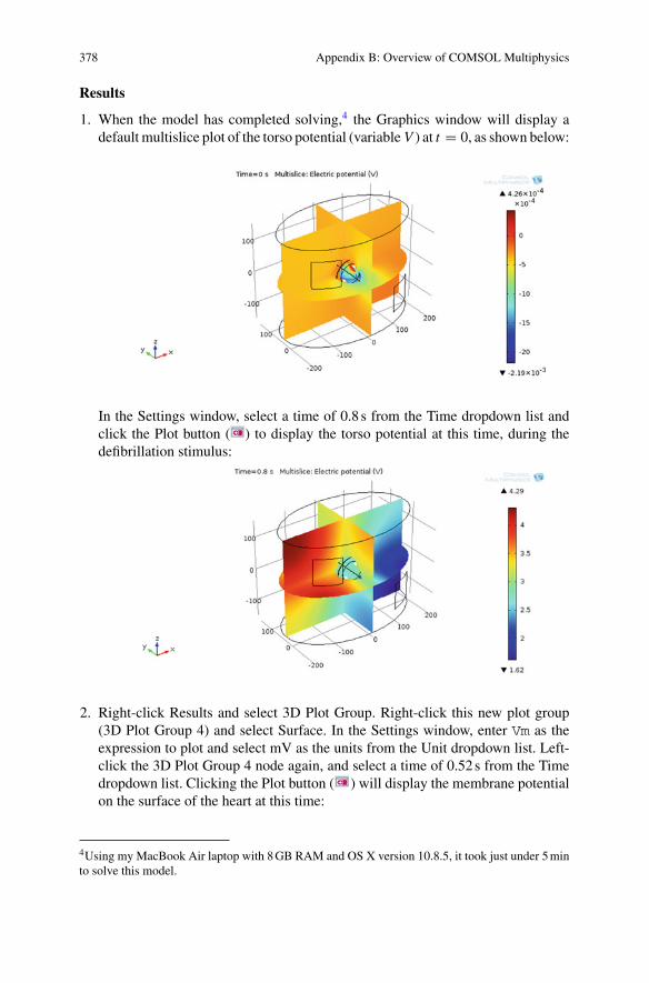
1. When the model has completed solving,4 the Graphics window will display adefault multislice plot of the torso potential (variable V ) at t = 0, as shown below:

In the Settings window, select a time of 0.8 s from the Time dropdown list andclick the Plot button ( ) to display the torso potential at this time, during thedefibrillation stimulus:

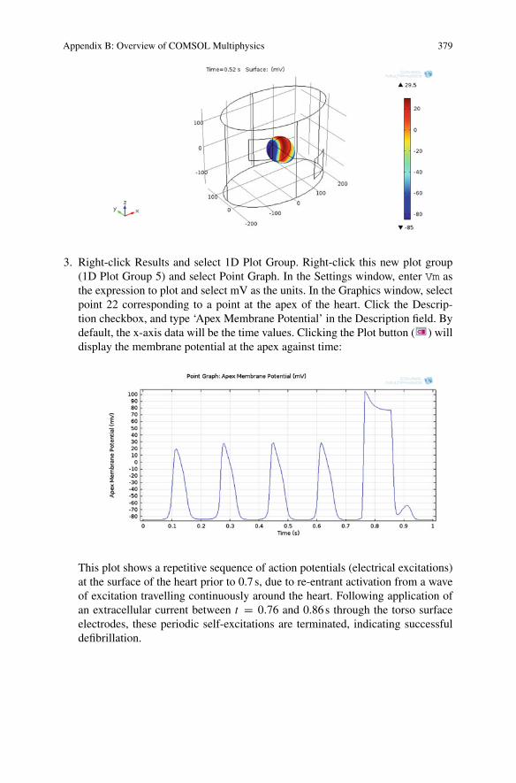
2. Right-click Results and select 3D Plot Group. Right-click this new plot group(3D Plot Group 4) and select Surface. In the Settings window, enter Vm as theexpression to plot and select mV as the units from the Unit dropdown list. Left-click the 3D Plot Group 4 node again, and select a time of 0.52 s from the Timedropdown list. Clicking the Plot button ( ) will display the membrane potentialon the surface of the heart at this time:

4Using my MacBook Air laptop with 8GB RAM and OS X version 10.8.5, it took just under 5minto solve this model.


3. Right-click Results and select 1D Plot Group. Right-click this new plot group(1D Plot Group 5) and select Point Graph. In the Settings window, enter Vm asthe expression to plot and select mV as the units. In the Graphics window, selectpoint 22 corresponding to a point at the apex of the heart. Click the Descrip-tion checkbox, and type ‘Apex Membrane Potential’ in the Description field. Bydefault, the x-axis data will be the time values. Clicking the Plot button ( ) willdisplay the membrane potential at the apex against time:

This plot shows a repetitive sequence of action potentials (electrical excitations)at the surface of the heart prior to 0.7 s, due to re-entrant activation from a waveof excitation travelling continuously around the heart. Following application ofan extracellular current between t = 0.76 and 0.86 s through the torso surfaceelectrodes, these periodic self-excitations are terminated, indicating successfuldefibrillation.

Solutions

Problems of Chap.1

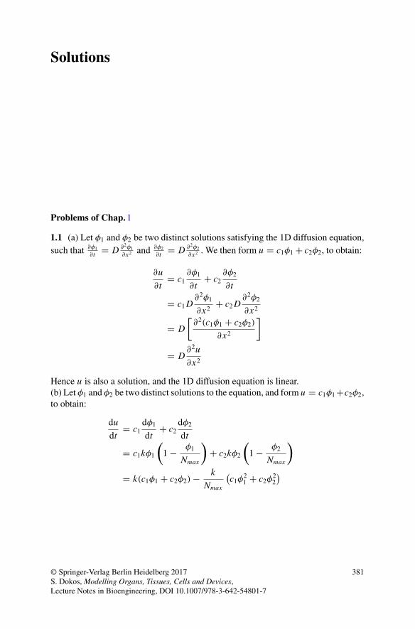
1.1 (a) Let φ1 and φ2 be two distinct solutions satisfying the 1D diffusion equation,such that ∂φ1

∂t = D ∂2φ1

∂x2 and ∂φ2

∂t = D ∂2φ2

∂x2 . We then form u = c1φ1 + c2φ2, to obtain:

∂u

∂t= c1

∂φ1

∂t+ c2

∂φ2

∂t

= c1D∂2φ1

∂x2+ c2D

∂2φ2

∂x2

= D

[∂2(c1φ1 + c2φ2)

∂x2

]

= D∂2u

∂x2

Hence u is also a solution, and the 1D diffusion equation is linear.(b) Let φ1 and φ2 be two distinct solutions to the equation, and form u = c1φ1+c2φ2,to obtain:

du

dt= c1

dφ1

dt+ c2

dφ2

dt

= c1kφ1

(1 − φ1

Nmax

)+ c2kφ2

(1 − φ2

Nmax

)

= k(c1φ1 + c2φ2) − k

Nmax

(c1φ

21 + c2φ

22

)


381

http://dx.doi.org/10.1007/978-3-642-54801-7_1

382 Solutions

= ku − k

Nmax

(u2 − u2 + c1φ

21 + c2φ

22

)

= ku − ku2

Nmax+ k

Nmax

(u2 + c1φ

21 + c2φ

22

)

= ku

(1 − u

Nmax

)+ k

Nmax

(u2 + c1φ

21 + c2φ

22

)

�= ku

(1 − u

Nmax

)

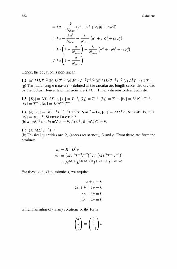
Hence, the equation is non-linear.

1.2 (a) MLT−2 (b) L2T−1 (c) M−1L−2T 4 I 2 (d) ML2T−3 I−2 (e) L3T−1 (f) T−1

(g) The radian angle measure is defined as the circular arc length subtended dividedby the radius. Hence its dimensions are L/L = 1, i.e. a dimensionless quantity.

1.3 [B0] = NL−3T−1, [k1] = T−1, [k2] = T−1, [k3] = T−1, [k4] = L3N−1T−1,[k5] = T−1, [k6] = L3N−1T−1.

1.4 (a) [c0] = ML−1T−2, SI units: Nm–2 = Pa, [c1] = ML8T , SI units: kgm8 s,[c2] = ML−1, SI units: Pa s2 rad–2

(b) a: mV–1 s–1, b: mV, c: mV, A: s–1, B: mV, C : mV.

1.5 (a) ML3T−3 I−2

(b) Physical quantities are Ra (access resistance), D and ρ. From these, we form theproducts

πi = RaaDbρc

[πi ] = (ML2T−3 I−2)a Lb

(ML3T−3 I−2)c

= M (a+c)L(2a+b+3c)T (−3a−3c) I (−2a−2c)

For these to be dimensionless, we require

a + c = 0

2a + b + 3c = 0

−3a − 3c = 0

−2a − 2c = 0

which has infinitely many solutions of the form

⎛⎝abc

⎞⎠ =

⎛⎝ 1

1−1

⎞⎠α

Solutions 383

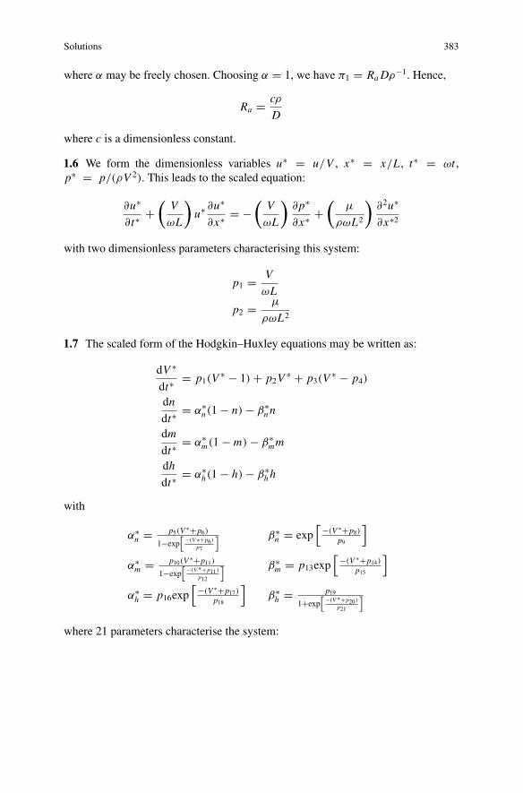
where α may be freely chosen. Choosing α = 1, we have π1 = RaDρ−1. Hence,

Ra = cρ

D

where c is a dimensionless constant.

1.6 We form the dimensionless variables u∗ = u/V , x∗ = x/L , t∗ = ωt ,p∗ = p/(ρV 2). This leads to the scaled equation:

∂u∗

∂t∗+(

V

ωL

)u∗ ∂u∗

∂x∗ = −(

V

ωL

)∂p∗

∂x∗ +(

μ

ρωL2

)∂2u∗

∂x∗2

with two dimensionless parameters characterising this system:

p1 = V

ωL

p2 = μ

ρωL2

1.7 The scaled form of the Hodgkin–Huxley equations may be written as:

dV ∗

dt∗= p1(V

∗ − 1) + p2V∗ + p3(V

∗ − p4)

dn

dt∗= α∗

n(1 − n) − β∗n n

dm

dt∗= α∗

m(1 − m) − β∗mm

dh

dt∗= α∗

h(1 − h) − β∗h h

with

α∗n = p5(V ∗+p6)

1−exp[ −(V∗+p6)

p7

] β∗n = exp

[−(V ∗+p8)p9

]

α∗m = p10(V ∗+p11)

1−exp[ −(V∗+p11)

p12

] β∗m = p13exp

[−(V ∗+p14)p15

]

α∗h = p16exp

[−(V ∗+p17)p18

]β∗h = p19

1+exp[ −(V∗+p20)

p21

]

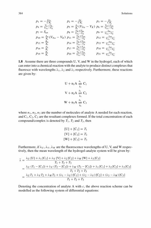
where 21 parameters characterise the system:

384 Solutions

p1 = − gNa

CBnp2 = − gK

CBnp3 = − gL

CBn

p4 = VL−VKVNa−VK

p5 = AnBn

(VNa − VK ) p6 = VK+VanVNa−VK

p7 = San p8 = VK+VbnVNa−VK

p9 = sbnVNa−VK

p10 = AmBn

(VNa − VK ) p11 = VK+VamVNa−VK

p12 = samVNa−VK

p13 = BmBn

p14 = VK+VbmVNa−VK

p15 = sbmVNa−VK

p16 = AhBn

p17 = VK+VahVNa−VK

p18 = sahVNa−VK

p19 = BhBn

p20 = VK+VbhVNa−VK

p21 = sbhVNa−VK

1.8 Assume there are three compounds U, V, and W in the hydrogel, each of whichcan enter into a chemical reaction with the analyte to produce distinct complexes thatfluoresce with wavelengths λ1, λ2 and λ3 respectively. Furthermore, these reactionsare given by:

U + n1Ak1−⇀↽−k2

C1

V + n2Ak3−⇀↽−k4

C2

W + n3Ak5−⇀↽−k6

C3

where n1, n2, n3 are the number of molecules of analyte A needed for each reaction,and C1, C2, C3 are the resultant complexes formed. If the total concentration of eachcompound/complex is denoted by T1, T2 and T3, then

[U] + [C1] = T1[V] + [C2] = T2[W] + [C3] = T3

Furthermore, if λU , λV , λW are the fluorescence wavelengths of U, V, and W respec-tively, then the mean wavelength of the hydrogel-analyte system will be given by:

λ = λU [U] + λ1 [C1] + λV [V] + λ2 [C2] + λW [W] + λ3 [C3]

T1 + T2 + T3

= λU (T1 − [C1]) + λV (T2 − [C2]) + λW (T3 − [C3]) + λ1 [C1] + λ2 [C2] + λ3 [C3]

T1 + T2 + T3

= λUT1 + λV T2 + λWT3 + (λ1 − λU ) [C1] + (λ2 − λV ) [C2] + (λ3 − λW ) [C3]

T1 + T2 + T3

Denoting the concentration of analyte A with c, the above reaction scheme can bemodelled as the following system of differential equations:

Solutions 385

d [C1]

dt= k1 [U] cn1 − k2 [C1] = k1 (T1 − [C1]) c

n1 − k2 [C1]

d [C2]

dt= k3 [V] cn2 − k4 [C2] = k3 (T2 − [C2]) c

n1 − k4 [C2]

d [C3]

dt= k5 [W] cn3 − k6 [C3] = k5 (T3 − [C3]) c

n1 − k6 [C3]

The steady-state concentrations of C1, C2, C3 can be found by equating the abovederivatives to zero, to obtain:

[C1] = T1cn1[cn1 + k2

k1

] , [C2] = T2cn2[cn2 + k4

k3

] , [C3] = T3cn3[cn3 + k6

k5

]

with the steady-state fluorescent wavelength given by:

λ = λ0 + F1(λ1 − λU )cn1[cn1 + k2

k1

] + F2(λ2 − λV )cn2[cn2 + k4

k3

] + F3(λ3 − λW )cn3[cn3 + k6

k5

]

where

λ0 = λUT1 + λV T2 + λWT3T1 + T2 + T3

, F1 = T1T1 + T2 + T3

, F2 = T2T1 + T2 + T3

,

F3 = T3T1 + T2 + T3

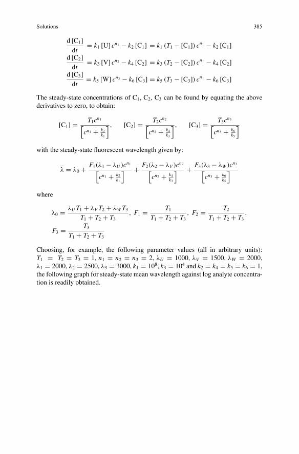
Choosing, for example, the following parameter values (all in arbitrary units):T1 = T2 = T3 = 1, n1 = n2 = n3 = 2, λU = 1000, λV = 1500, λW = 2000,λ1 = 2000, λ2 = 2500, λ3 = 3000, k1 = 108, k3 = 104 and k2 = k4 = k5 = k6 = 1,the following graph for steady-state mean wavelength against log analyte concentra-tion is readily obtained.

386 Solutions

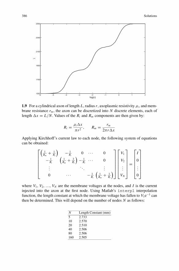
1.9 For a cylindrical axon of length L , radius r , axoplasmic resistivity ρi , and mem-brane resistance rm , the axon can be discretized into N discrete elements, each oflength x = L/N . Values of the Ri and Rm components are then given by:

Ri = ρi x

πr2, Rm = rm

2πr x

Applying Kirchhoff’s current law to each node, the following system of equationscan be obtained:

⎡⎢⎢⎢⎢⎢⎢⎣

(1Rm

+ 1Ri

)− 1

Ri0 · · · 0

− 1Ri

(1Rm

+ 2Ri

)− 1

Ri· · · 0

.... . .

...

0 · · · − 1Ri

(1Rm

+ 1Ri

)

⎤⎥⎥⎥⎥⎥⎥⎦

⎡⎢⎢⎢⎢⎢⎢⎣

V1

V2

...

VN

⎤⎥⎥⎥⎥⎥⎥⎦

=

⎡⎢⎢⎢⎢⎢⎢⎣

I

0...

0

⎤⎥⎥⎥⎥⎥⎥⎦

where V1, V2, …, VN are the membrane voltages at the nodes, and I is the currentinjected into the axon at the first node. Using Matlab’s interp1 interpolationfunction, the length constant at which the membrane voltage has fallen to V1e−1 canthen be determined. This will depend on the number of nodes N as follows:

N Length Constant (mm)5 2.73310 2.57020 2.51040 2.50680 2.506160 2.505

Solutions 387

N = 20 is sufficient to yield a length constant accuracy of 1%.

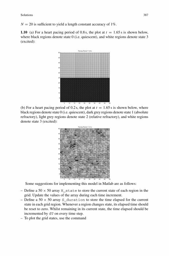
1.10 (a) For a heart pacing period of 0.8 s, the plot at t = 1.65 s is shown below,where black regions denote state 0 (i.e. quiescent), and white regions denote state 3(excited):

5 10 15 20 25 30 35 40 45 50

5

10

15

20

25

30

35

40

45

50Pacing Period = 0.8 s

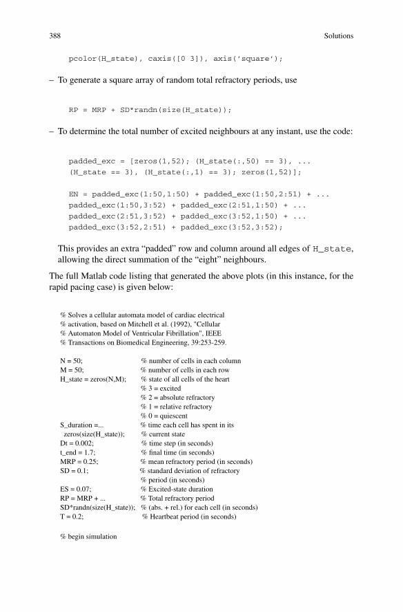
(b) For a heart pacing period of 0.2 s, the plot at t = 1.65 s is shown below, whereblack regions denote state 0 (i.e. quiescent), dark grey regions denote state 1 (absoluterefractory), light grey regions denote state 2 (relative refractory), and white regionsdenote state 3 (excited):

5 10 15 20 25 30 35 40 45 50

5

10

15

20

25

30

35

40

45

50Pacing Period = 0.2 s

Some suggestions for implementing this model in Matlab are as follows:

– Define a 50 × 50 array H_state to store the current state of each region in thegrid. Update the values of the array during each time increment.

– Define a 50 × 50 array S_duration to store the time elapsed for the currentstate in each grid region. Whenever a region changes state, its elapsed time shouldbe reset to zero. Whilst remaining in its current state, the time elapsed should beincremented by dT on every time step.

– To plot the grid states, use the command

388 Solutions

pcolor(H_state), caxis([0 3]), axis(’square’);

– To generate a square array of random total refractory periods, use

RP = MRP + SD*randn(size(H_state));

– To determine the total number of excited neighbours at any instant, use the code:

padded_exc = [zeros(1,52); (H_state(:,50) == 3), ...

(H_state == 3), (H_state(:,1) == 3); zeros(1,52)];

EN = padded_exc(1:50,1:50) + padded_exc(1:50,2:51) + ...

padded_exc(1:50,3:52) + padded_exc(2:51,1:50) + ...

padded_exc(2:51,3:52) + padded_exc(3:52,1:50) + ...

padded_exc(3:52,2:51) + padded_exc(3:52,3:52);

This provides an extra “padded” row and column around all edges of H_state,allowing the direct summation of the “eight” neighbours.

The full Matlab code listing that generated the above plots (in this instance, for therapid pacing case) is given below:

% Solves a cellular automata model of cardiac electrical% activation, based on Mitchell et al. (1992), "Cellular% Automaton Model of Ventricular Fibrillation", IEEE% Transactions on Biomedical Engineering, 39:253-259.

N = 50; % number of cells in each columnM = 50; % number of cells in each rowH_state = zeros(N,M); % state of all cells of the heart

% 3 = excited% 2 = absolute refractory% 1 = relative refractory% 0 = quiescent

S_duration =... % time each cell has spent in itszeros(size(H_state)); % current state

Dt = 0.002; % time step (in seconds)t_end = 1.7; % final time (in seconds)MRP = 0.25; % mean refractory period (in seconds)SD = 0.1; % standard deviation of refractory

% period (in seconds)ES = 0.07; % Excited-state durationRP = MRP + ... % Total refractory periodSD*randn(size(H_state)); % (abs. + rel.) for each cell (in seconds)T = 0.2; % Heartbeat period (in seconds)

% begin simulation

Solutions 389

for t = 0:Dt:t_end% determine number of excited neighbours for each cellpadded_exc = [zeros(1,M+2); (H_state(:,M) == 3), ...(H_state == 3), (H_state(:,1) == 3); zeros(1,M+2)];

EN = padded_exc(1:N,1:M) + padded_exc(1:N,2:M+1) + ...padded_exc(1:N,3:M+2) + padded_exc(2:N+1,1:M) + ...padded_exc(2:N+1,3:M+2) + padded_exc(3:N+2,1:M) + ...padded_exc(3:N+2,2:M+1) + padded_exc(3:N+2,3:M+2);

% calculate spread of activationfor i = 1:Mfor j = 1:N

if (H_state(i,j) == 0) % if quiescentif (EN(i,j) > 0)

H_state(i,j) = 3;S_duration(i,j) = 0;

elseS_duration(i,j) = S_duration(i,j) + Dt;

end;elseif (H_state(i,j) == 3) % if excitedif (S_duration(i,j) >= ES)



end;elseif (H_state(i,j) == 2) % if absolute refractoryif (S_duration(i,j) >= RP(i,j)-0.05)



end;else % if relative refractoryif ((S_duration(i,j) <= 0.002)&&(EN(i,j) == 8))


elseif ((S_duration(i,j) <= 0.004)&&(EN(i,j) >= 7))H_state(i,j) = 3;S_duration(i,j) = 0;





elseif ((S_duration(i,j) <= 0.05)&&(EN(i,j) >= 2))

390 Solutions


elseif ((S_duration(i,j) > 0.05)&&(EN(i,j) >= 1))H_state(i,j) = 3;S_duration(i,j) = 0;

elseif (S_duration(i,j) > 0.05)H_state(i,j) = 0;S_duration(i,j) = 0;


end;end;

end; % j loopend; % i loop% if necessary, excite the pacemaker cellif (mod(t,T) < Dt)if (H_state(N,round(M/4)) ˜= 2)

H_state(N,round(M/4)) = 3;S_duration(N,round(M/4)) = 0;

end;end;

% plot statespause(0.1);pcolor(H_state), caxis([0 3]), axis(’square’), ...title(’Simulation of Cardiac Electrical Activity ’);

end; % t loop

Problems of Chap.2

2.1 (a) To solve dxdt = αx (1 − x) − βx x , we re-write it as the non-homogeneous

linear equation:dx

dt+ (αx + βx )x = αx

To solve this ODE, we first solve the homogeneous form

dx

dt+ (αx + βx )x = 0

with characteristic equation

m + (αx + βx ) = 0

∴ m = −(αx + βx )

Hence, the homogeneous solution is

xh = Ce−(αx+βx )t

http://dx.doi.org/10.1007/978-3-642-54801-7_2

Solutions 391

where C is a constant.Next, we solve for a particular solution, which we can conveniently take as thesteady-state value of x . This steady-state value can be obtained from the originalnon-homogeneous ODE by simply setting dx

dt = 0,

⇒ (αx + βx )x = αx

Hence, a particular solution is

xp = αx

αx + βx

The general solution is the sum of the homogeneous and particular solutions:

x = Ce−(αx+βx )t + αx

αx + βx

When t = 0, x = x0

∴ x0 = C + αx

αx + βx

⇒ C = x0 − αx

αx + βx

Thus, the solution of the ODE is

x =[x0 − αx

αx + βx

]e−(αx+βx )t + αx

αx + βx

(b) From above, the steady-state solution, x∞, is given by

x∞ = αx

αx + βx

and since αx , βx are functions of the membrane potential, which equals Vclamp duringthe voltage-clamp, this steady state value is more accurately expressed as

x∞ = αx (Vclamp)

αx (Vclamp) + βx (Vclamp)

Hence, a reasonable estimate for x0 would be the corresponding steady-state valueat the holding potential Vhold , prior to the onset of the voltage-clamp step, or

x0 = αx (Vhold)

αx (Vhold) + βx (Vhold)

2.2 (a) The total force applied to the muscle is given by

392 Solutions

F = k1x1 = bdx2dt

+ k2x2

and since the total length x is held fixed at Xm , then x1 = Xm − x2. Substituting thisvalue for x1 into the right-most equality above, we have:

bdx2dt

+ k2x2 = k1 [Xm − x2]

bdx2dt

+ (k1 + k2)x2 = k1Xm

ordx2dt

+(k1 + k2

b

)x2 = k1

bXm

To solve this ODE, the corresponding homogeneous equation is

dx2dt

+(k1 + k2

b

)x2 = 0

with homogeneous solution

x2,h = Ce−(

k1+k2b

)t

where C is a constant. A particular solution can be found for the steady-state valueof x2 by setting dx2

dt = 0 in the non-homogeneous ODE. This yields the particularsolution

x2,p =(

k1k1 + k2

)Xm

Hence, the general solution is the sum of the homogeneous and particular solutions:

x2 = Ce−(

k1+k2b

)t +

(k1

k1 + k2

)Xm

When t = 0, x2 = 0, which implies C = −(

k1k1+k2

)Xm . Hence

x2 =(

k1k1 + k2

)Xm

[1 − e

−(

k1+k2b

)t]

Knowing x2, we can readily obtain x1:

x1 = Xm − x2

=(

k2k1 + k2

)Xm +

(k1

k1 + k2

)Xme

−(

k1+k2b

)t

=(

Xm

k1 + k2

)[k2 + k1e

−(

k1+k2b

)t]

Solutions 393

Since F = k1x1, the applied force is readily determined as

F =(

k1Xm

k1 + k2

)[k2 + k1e

−(

k1+k2b

)t]

(b) The fixed applied force, Fm , satisfies

Fm = k1x1 = bdx2dt

+ k2x2

and working with variable x2, we can rewrite the above as

dx2dt

+ k2bx2 = Fm

b

The homogeneous ODE isdx2dt

+ k2bx2 = 0

with solution

x2,h = Ce−(

k2b

)t

where C is a constant. The particular solution can be found from the steady-statevalue of x2 in the non-homogeneous ODE by setting dx2

dt = 0. We therefore obtainthe particular solution

x2,p = Fm

k2

and the general solution

x2 = Ce−(

k2b

)t + Fm

k2

When t = 0, x2 = 0, which implies C = − Fmk2. Hence

x2 = Fm

k2

[1 − e

−(

k2b

)t]

Furthermore, since Fm = k1x1, we have x1 = Fm/k1. Hence, the total length of themuscle is given by

x = x1 + x2 = Fm

[1

k1+ 1

k2− 1

k2e−(

k2b

)t]

2.3 (a) The total current flowing through the parallel resistive and capacitivebranches is equal to the applied stimulus current. Hence, the ODE for this system isgiven by

394 Solutions

CdV

dt+ V

R= I

ordV

dt+ V

RC= I

C

The homogeneous ODE for this system is

dV

dt+ V

RC= 0

with homogeneous solution Vh = Ce− tRC , where C is a constant. The particular

solution, V2,p, can be obtained by setting dVdt = 0 in the original ODE to obtain:

V2,p = I R

Hence, the general solution, given by the sum of the homogeneous and particularsolutions, is

V = I R + Ce− tRC

When t = 0, V = 0, which implies C = −I R. Hence,

V = I R(1 − e− t

RC

)

Now, when V = Vth , the required stimulus duration T must therefore satisfy

Vth = I R(1 − e− T

RC

)

Hence, the strength-duration characteristic is

I = Vth

R(1 − e− T

RC

)

(b) From the strength-duration characteristic above, the rheobase may be found fromthe stimulus current I as T → ∞, or simply

Irheobase = Vth

R

The chronaxie can be found by solving for stimulus duration T corresponding to anapplied current of 2Irheobase. From the previous strength-duration characteristic, wehave:

Solutions 395

2Vth

R= Vth

R(1 − e− T

RC

)

2 = 1

1 − e− TRC

1 − e− TRC = 1

2

e− TRC = 1

2T

RC= ln 2

∴ Tchronaxie = RC ln 2

≈ 0.69RC

2.4 (a) The pair of ODEs describing the coupled spring masses is

Mx1 = −kx1 + k(x2 − x1)

Mx2 = k(x1 − x2) − kx2

or

Mx1 = −2kx1 + kx2Mx2 = kx1 − 2kx2

(b) Adding the above ODEs together produces

Mx1 + Mx2 = −kx1 − kx2

or simplyMy1 = −ky1

where we have used the substitution y1 = x1 + x2. To solve this ODE, we can writeits characteristic equation as

Mm2 + k = 0

⇒ m = ±i

√k

M

Hence,

y1 = C1ei t√

kM + C2e

−i t√

kM

= C1 cos

(t

√k

M

)+ C1i sin

(t

√k

M

)+ C2 cos

(t

√k

M

)− C2i sin

(t

√k

M

)

396 Solutions

where C1 and C2 are constants. Differentiating this expression, we obtain

y1 = − C1

√k

Msin

(t

√k

M

)+ C1

√k

Mi cos

(t

√k

M

)

− C2

√k

Msin

(t

√k

M

)− C2

√k

Mi cos

(t

√k

M

)

When t = 0, y1 = u1 + u2 and y1 = x1 + x2 = 0. Substituting these into the aboveequations for y1 and y1 yields

u1 + u2 = C1 + C2

0 = C1

√k

Mi − C2

√k

Mi

or

C1 = C2 = 1

2(u1 + u2)

Hence,

y1 = (u1 + u2) cos

(t

√k

M

)

Similarly, we can subtract the two original ODEs in x1 and x2 to obtain:

Mx1 − Mx2 = −3kx1 + 3kx2

orMy2 = −3ky2

where we have used the substitution y2 = x1 − x2. The characteristic equation ofthis ODE is

Mm2 + 3k = 0

⇒ m = ±i

√3k

M

Hence,

y2 = C3ei t√

3kM + C4e

−i t√

3kM

= C3 cos

(t

√3k

M

)+ C3i sin

(t

√3k

M

)+ C4 cos

(t

√3k

M

)− C4i sin

(t

√3k

M

)

where C3 and C4 are constants. Differentiating this expression, we obtain

Solutions 397

y2 = − C3

√3k

Msin

(t

√3k

M

)+ C3

√3k

Mi cos

(t

√3k

M

)

− C4

√3k

Msin

(t

√3k

M

)− C4

√3k

Mi cos

(t

√3k

M

)

When t = 0, y2 = u1 − u2 and y2 = x1 − x2 = 0. Substituting these into the aboveequations for y2 and y2 yields

u1 − u2 = C3 + C4

0 = C3

√3k

Mi − C4

√3k

Mi

or

C3 = C4 = 1

2(u1 − u2)

Hence,

y2 = (u1 − u2) cos

(t

√3k

M

)

To recover x1 and x2 from y1 and y2, we can use the expressions

x1 = 1

2(y1 + y2)

x2 = 1

2(y1 − y2)

to finally obtain

x1 = 1

2(u1 + u2) cos

(t

√k

M

)+ 1

2(u1 − u2) cos

(t

√3k

M

)

x2 = 1

2(u1 + u2) cos

(t

√k

M

)− 1

2(u1 − u2) cos

(t

√3k

M

)

2.5 The ODEs for the glucose-insulin model are

dI

dt= k2 Ip(t) − k3 I

dG

dt= B0 − (k1 + k4 I + k5 + k6 I )

The followingMatlab code (GI_solve.m andGI_prime.m)will numerically-integratethese and display the solution:

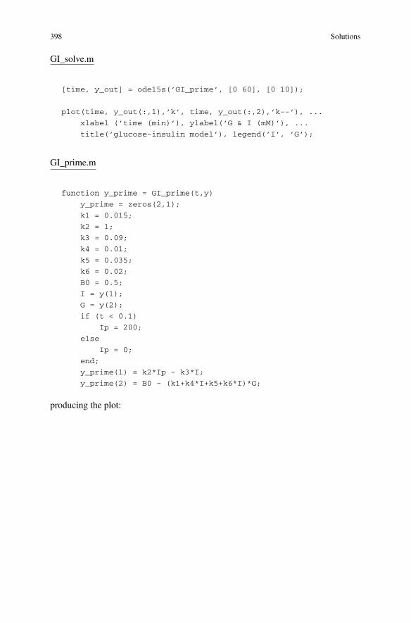
398 Solutions

GI_solve.m

[time, y_out] = ode15s(’GI_prime’, [0 60], [0 10]);

plot(time, y_out(:,1),’k’, time, y_out(:,2),’k--’), ...

xlabel (’time (min)’), ylabel(’G & I (mM)’), ...

title(’glucose-insulin model’), legend(’I’, ’G’);

GI_prime.m

function y_prime = GI_prime(t,y)

y_prime = zeros(2,1);

k1 = 0.015;

k2 = 1;

k3 = 0.09;

k4 = 0.01;

k5 = 0.035;

k6 = 0.02;

B0 = 0.5;

I = y(1);

G = y(2);

if (t < 0.1)

Ip = 200;

else

Ip = 0;

end;

y_prime(1) = k2*Ip - k3*I;

y_prime(2) = B0 - (k1+k4*I+k5+k6*I)*G;

producing the plot:

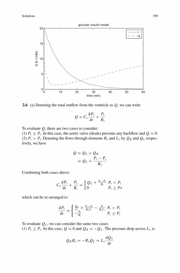
Solutions 399

0 10 20 30 40 50 600

5

10

15

20

time (min)

G &

I (m

M)

glucose−insulin model

IG

2.6 (a) Denoting the total outflow from the ventricle as Q, we can write

Q = CsdPsdt

+ PsRs

To evaluate Q, there are two cases to consider:(1) Pv ≤ Ps . In this case, the aortic valve (diode) prevents any backflow and Q = 0.(2) Pv > Ps . Denoting the flows through elements Ro and Lo by QR and QL respec-tively, we have

Q = QL + QR

= QL + Pv − PsRo

Combining both cases above:

CsdPsdt

+ PsRs

={QL + Pv−Ps

RoPv > Ps

0 Pv ≤ Ps

which can be re-arranged to

dPsdt

={

QL

Cs+ Pv−Ps

RoCs− Ps

RsCsPv > Ps

− PsRs

Pv ≤ Ps

To evaluate QL , we can consider the same two cases:(1) Pv ≤ Ps . In this case, Q = 0 and QR = −QL . The pressure drop across Lo is

QRRo = −RoQL = LodQL

dt

400 Solutions

Hence,dQL

dt= − Ro

LoQL

(2) Pv > Ps . In this case, the pressure drop across Lo is given by:

Pv − Ps = LodQL

dt

∴ dQL

dt= Pv − Ps

Lo

Hence, the pair of ODEs characterising the system is

dPsdt

={

QL

Cs+ Pv−Ps

RoCs− Ps

RsCsPv > Ps

− PsRs

Pv ≤ Ps

dQL

dt=

{Pv−PsLo

Pv > Ps

− RoLoQL Pv ≤ Ps

(b) The followingMatlab code (Windkessel_solve.m andWindkessel_prime.m) willsolve these ODEs over a time interval of 100T (i.e. 100 heartbeats) to obtain a suffi-cient steady-state Ps waveform, then use the final state variable values as subsequentinitial values to solve for a further time interval of T . The initial values for Ps andQL are both zero at the start of the 100T simulation:

Windkessel_solve.m

% define global parameters

global R0 L0 Cs Rs P T tc

R0 = 0.06; % mmHg.s/cmˆ3

L0 = 0.2; % mmHg.sˆ2/cmˆ3

Cs = 1; % cmˆ3/mmHg

Rs = 1.4; % mmHg.s/cmˆ3

P = 120; % mmHg

T = 1; % s

tc = 0.35; % s

% solve first for 100 heartbeats

Ps_init = 0;

QL_init = 0;

[time, y_out] = ode15s(’Windkessel_prime’, ...

[0 100*T], [Ps_init QL_init]);

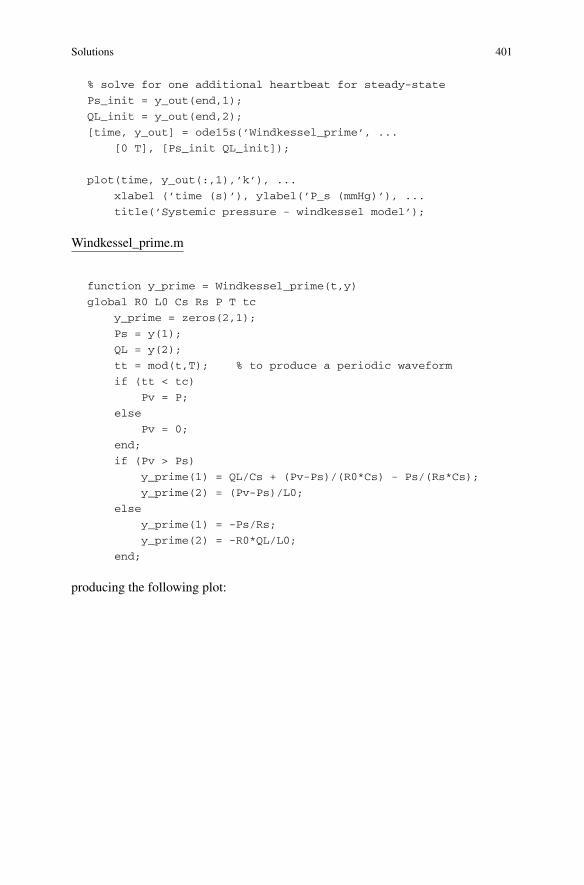
Solutions 401

% solve for one additional heartbeat for steady-state

Ps_init = y_out(end,1);

QL_init = y_out(end,2);

[time, y_out] = ode15s(’Windkessel_prime’, ...

[0 T], [Ps_init QL_init]);

plot(time, y_out(:,1),’k’), ...

xlabel (’time (s)’), ylabel(’P_s (mmHg)’), ...

title(’Systemic pressure - windkessel model’);

Windkessel_prime.m

function y_prime = Windkessel_prime(t,y)

global R0 L0 Cs Rs P T tc


Ps = y(1);

QL = y(2);

tt = mod(t,T); % to produce a periodic waveform

if (tt < tc)

Pv = P;

else

Pv = 0;

end;

if (Pv > Ps)

y_prime(1) = QL/Cs + (Pv-Ps)/(R0*Cs) - Ps/(Rs*Cs);

y_prime(2) = (Pv-Ps)/L0;

else

y_prime(1) = -Ps/Rs;

y_prime(2) = -R0*QL/L0;

end;

producing the following plot:

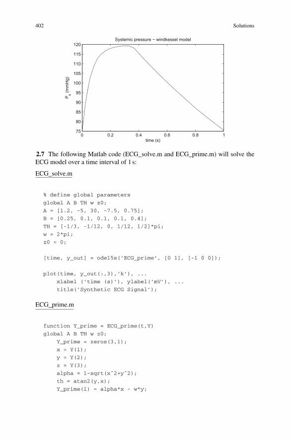
402 Solutions

0 0.2 0.4 0.6 0.8 175

80

85

90

95

100

105

110

115

120

time (s)

Ps (m

mH

g)

Systemic pressure − windkessel model

2.7 The following Matlab code (ECG_solve.m and ECG_prime.m) will solve theECG model over a time interval of 1 s:

ECG_solve.m

% define global parameters

global A B TH w z0;

A = [1.2, -5, 30, -7.5, 0.75];

B = [0.25, 0.1, 0.1, 0.1, 0.4];

TH = [-1/3, -1/12, 0, 1/12, 1/2]*pi;

w = 2*pi;

z0 = 0;

[time, y_out] = ode15s(’ECG_prime’, [0 1], [-1 0 0]);

plot(time, y_out(:,3),’k’), ...

xlabel (’time (s)’), ylabel(’mV’), ...

title(’Synthetic ECG Signal’);

ECG_prime.m

function Y_prime = ECG_prime(t,Y)

global A B TH w z0;

Y_prime = zeros(3,1);

x = Y(1);

y = Y(2);

z = Y(3);

alpha = 1-sqrt(xˆ2+yˆ2);

th = atan2(y,x);

Y_prime(1) = alpha*x - w*y;

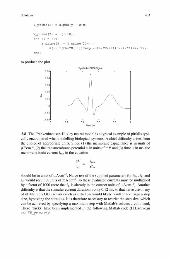
Solutions 403

Y_prime(2) = alpha*y + w*x;

Y_prime(3) = -(z-z0);

for ii = 1:5

Y_prime(3) = Y_prime(3)-...

A(ii)*(th-TH(ii))*exp(-(th-TH(ii))ˆ2/(2*B(ii)ˆ2));

end;

to produce the plot

0 0.2 0.4 0.6 0.8 1−0.02

−0.01

0

0.01

0.02

0.03

0.04

0.05

time (s)

mV

Synthetic ECG Signal

2.8 The Frankenhaeuser–Huxley neural model is a typical example of pitfalls typi-cally encountered when modelling biological systems. A chief difficulty arises fromthe choice of appropriate units. Since (1) the membrane capacitance is in units ofμFcm–2, (2) the transmembrane potential is in units of mV and (3) time is in ms, themembrane ionic current iion in the equation

dV

dt= − iion

Cm

should be in units of μAcm–2. Naive use of the supplied parameters for iNa , iK andiP would result in units of mAcm–2, so these evaluated currents must be multipliedby a factor of 1000 (note that iL is already in the correct units of μAcm–2). Anotherdifficulty is that the stimulus current duration is only 0.12ms, so that naive use of anyof of Matlab’s ODE solvers such as ode15s would likely result in too large a stepsize, bypassing the stimulus. It is therefore necessary to restrict the step size, whichcan be achieved by specifying a maximum step with Matlab’s odeset command.These ‘tricks’ have been implemented in the following Matlab code (FH_solve.mand FH_prime.m):

404 Solutions

FH_solve.m

% solves the Frankenhaeuser--Huxley neural modelglobal Cm P_Na P_K P_P g_L V_L Na_o;global Na_i K_o K_i I_s t_on t_dur;global Er F R T;

Cm = 2; % uC/cmˆ2P_Na = 0.008; % cm/sP_K = 0.0012; % cm/sP_P = 0.00054; % cm/sg_L = 30.3; % mS/cmˆ2V_L = 0.026; % mVNa_o = 114.5; % mMNa_i = 13.74; % mMK_o = 2.5; % mMK_i = 120; % mMI_s = 1; % mA/cmˆ2t_on = 1; % mst_dur = 0.12; % msEr = -70; % mVF = 96.49; % C/mmolR = 8.31; % J/(mol*K)T = 310; % K

Y_init = [0, 0.0005, 0.8249, 0.0268, 0.0049];options = odeset(’MaxStep’, 0.01);% solve first for control case (no TTX)[time_1, Y_out_1] = ode15s(’FH_prime’, [0 5], Y_init, options);% next, solve for presence of TTXP_Na = 0.2*P_Na;[time_2, Y_out_2] = ode15s(’FH_prime’, [0 5], Y_init, options);plot(time_1, Y_out_1(:,1)+Er, ’k’, time_2, Y_out_2(:,1)+Er, ’k--’), ...

xlabel(’ms’), ylabel(’mV’), legend(’Control’, ’TTX’), ...title(’TTX effect on neural action potential’);

FH_prime.m

function y_out = FH_prime(t,y)

% calculates derivatives for solving the

% Frankenhaeuser--Huxley neural model.

global Cm P_Na P_K P_P g_L V_L Na_o;

global Na_i K_o K_i I_s t_on t_dur;

global Er F R T;

y_out = zeros(5,1);

V = y(1);

m = y(2);

h = y(3);

n = y(4);

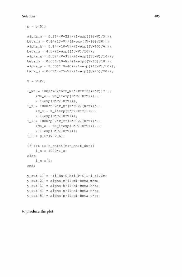
Solutions 405

p = y(5);

alpha_m = 0.36*(V-22)/(1-exp((22-V)/3));

beta_m = 0.4*(13-V)/(1-exp((V-13)/20));

alpha_h = 0.1*(-10-V)/(1-exp((V+10)/6));

beta_h = 4.5/(1+exp((45-V)/10));

alpha_n = 0.02*(V-35)/(1-exp((35-V)/10));

beta_n = 0.05*(10-V)/(1-exp((V-10)/10));

alpha_p = 0.006*(V-40)/(1-exp((40-V)/10));

beta_p = 0.09*(-25-V)/(1-exp((V+25)/20));

E = V+Er;

i_Na = 1000*mˆ2*h*P_Na*(E*Fˆ2/(R*T))*...

(Na_o - Na_i*exp(E*F/(R*T)))...

/(1-exp(E*F/(R*T)));

i_K = 1000*nˆ2*P_K*(E*Fˆ2/(R*T))*...

(K_o - K_i*exp(E*F/(R*T)))...

/(1-exp(E*F/(R*T)));

i_P = 1000*pˆ2*P_P*(E*Fˆ2/(R*T))*...

(Na_o - Na_i*exp(E*F/(R*T)))...

/(1-exp(E*F/(R*T)));

i_L = g_L*(V-V_L);

if ((t >= t_on)&&(t<t_on+t_dur))

i_s = 1000*I_s;

else

i_s = 0;

end;

y_out(1) = -(i_Na+i_K+i_P+i_L-i_s)/Cm;

y_out(2) = alpha_m*(1-m)-beta_m*m;

y_out(3) = alpha_h*(1-h)-beta_h*h;

y_out(4) = alpha_n*(1-n)-beta_n*n;

y_out(5) = alpha_p*(1-p)-beta_p*p;

to produce the plot

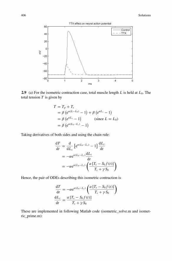
406 Solutions

0 1 2 3 4 5−80

−60

−40

−20

0

20

40

60

ms

mV

TTX effect on neural action potential

ControlTTX

2.9 (a) For the isometric contraction case, total muscle length L is held at L0. Thetotal tension T is given by

T = Tp + Ts= β

(eα(L−L0) − 1

) + β(eαLs − 1

)= β

(eαLs − 1

)(since L = L0)

= β(eα(L0−Lc) − 1

)

Taking derivatives of both sides and using the chain rule:

dT

dt= d

dLc

[eα(L0−Lc) − 1

] dLc

dt

= −αeα(L0−Lc)dLc

dt

= −αeα(L0−Lc)

(a [Ts − S0 f (t)]

Ts + γ S0

)

Hence, the pair of ODEs describing this isometric contraction is

dT

dt= −αeα(L0−Lc)

(a [Ts − S0 f (t)]

Ts + γ S0

)

dLc

dt= a [Ts − S0 f (t)]

Ts + γ S0

These are implemented in following Matlab code (isometric_solve.m and isomet-ric_prime.m):

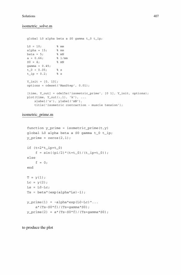
Solutions 407

isometric_solve.m

global L0 alpha beta a S0 gamma t_0 t_ip;

L0 = 10; % mmalpha = 15; % mmbeta = 5; % mNa = 0.66; % 1/mmS0 = 4; % mNgamma = 0.45;t_0 = 0.05; % st_ip = 0.2; % s

Y_init = [0, 10];options = odeset(’MaxStep’, 0.01);

[time, Y_out] = ode15s(’isometric_prime’, [0 1], Y_init, options);plot(time, Y_out(:,1), ’k’), ...

xlabel(’s’), ylabel(’mN’),title(’Isometric contraction - muscle tension’);

isometric_prime.m

function y_prime = isometric_prime(t,y)



if (t<2*t_ip+t_0)

f = sin((pi/2)*(t+t_0)/(t_ip+t_0));

else

f = 0;

end

T = y(1);

Lc = y(2);

Ls = L0-Lc;

Ts = beta*(exp(alpha*Ls)-1);

y_prime(1) = -alpha*exp(L0-Lc)*...

a*(Ts-S0*f)/(Ts+gamma*S0);

y_prime(2) = a*(Ts-S0*f)/(Ts+gamma*S0);

to produce the plot

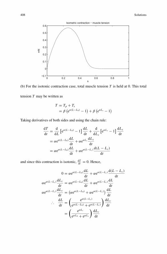
408 Solutions

0 0.2 0.4 0.6 0.8 1−0.1

0

0.1

0.2

0.3

0.4

0.5

0.6

s

mN

Isometric contraction − muscle tension

(b) For the isotonic contraction case, total muscle tension T is held at 0. This total

tension T may be written as

T = Tp + Ts= β

(eα(L−L0) − 1

) + β(eαLs − 1

)

Taking derivatives of both sides and using the chain rule:

dT

dt= d

dL

[eα(L−L0) − 1

] dLdt

+ d

dLs

[eαLs − 1

] dLs

dt

= αeα(L−L0)dL

dt+ αeαLs

dLs

dt

= αeα(L−L0)dL

dt+ αeα(L−Lc)

d(L − Lc)

dt

and since this contraction is isotonic, dTdt = 0. Hence,

0 = αeα(L−L0)dL

dt+ αeα(L−Lc)

d(L − Lc)

dt

αeα(L−Lc)dLc

dt= αeα(L−L0)

dL

dt+ αeα(L−Lc)

dL

dt

αeα(L−Lc)dLc

dt= (

αeα(L−L0) + αeα(L−Lc)) dLdt

∴ dL

dt=

(eα(L−Lc)

eα(L−L0) + eα(L−Lc)

)dLc

dt

=(

eαLc

eαL0 + eαLc

)dLc

dt

Solutions 409

=(

eαLc

eαL0 + eαLc

)a [Ts − S0 f (t)]

Ts + γ S0

Hence, the pair of ODEs describing the isotonic contraction is

dL

dt=

(eαLc

eαL0 + eαLc

)a [Ts − S0 f (t)]

Ts + γ S0dLc

dt= a [Ts − S0 f (t)]

Ts + γ S0

These are implemented in following Matlab code (isotonic_solve.m andisotonic_prime.m):

isotonic_solve.m


L0 = 10; % mmalpha = 15; % mmbeta = 5; % mNa = 0.66; % 1/mmS0 = 4; % mNgamma = 0.45;t_0 = 0.05; % st_ip = 0.2; % s

Y_init = [10, 10];options = odeset(’MaxStep’, 0.01);

[time, Y_out] = ode15s(’isotonic_prime’, [0 1], Y_init, options);plot(time, Y_out(:,1), ’k’), ...

xlabel(’s’), ylabel(’mm’),title(’Isotonic contraction - muscle length’);

isotonic_prime.m

function y_prime = isotonic_prime(t,y)



if (t<2*t_ip+t_0)

f = sin((pi/2)*(t+t_0)/(t_ip+t_0));

else

f = 0;

end

L = y(1);

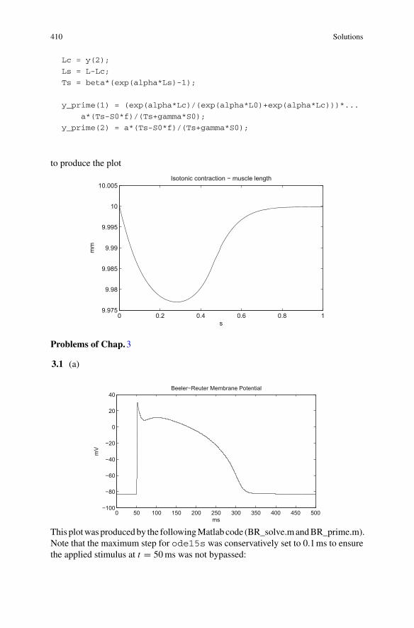
410 Solutions

Lc = y(2);

Ls = L-Lc;

Ts = beta*(exp(alpha*Ls)-1);

y_prime(1) = (exp(alpha*Lc)/(exp(alpha*L0)+exp(alpha*Lc)))*...

a*(Ts-S0*f)/(Ts+gamma*S0);

y_prime(2) = a*(Ts-S0*f)/(Ts+gamma*S0);

to produce the plot

0 0.2 0.4 0.6 0.8 19.975

9.98

9.985

9.99

9.995

10

10.005

s

mm

Isotonic contraction − muscle length

Problems of Chap.3

3.1 (a)

0 50 100 150 200 250 300 350 400 450 500−100

−80

−60

−40

−20

0

20

40

ms

mV

Beeler−Reuter Membrane Potential

This plotwasproducedby the followingMatlab code (BR_solve.mandBR_prime.m).Note that the maximum step for ode15s was conservatively set to 0.1ms to ensurethe applied stimulus at t = 50ms was not bypassed:

http://dx.doi.org/10.1007/978-3-642-54801-7_3

Solutions 411

BR_solve.m

% solves the Beeler-Reuter (1977) modelglobal Cm r_Ca Ca_SR k_up A_K1 A_x1 g_Na;global g_NaC V_Na g_s A_s t_on t_dur;

Cm = 1; % uC/cmˆ2r_Ca = 1e-7; % M*cmˆ2/nCCa_SR = 1e-7; % Mk_up = 0.07; % 1/msA_K1 = 0.35; % uA/cmˆ2A_x1 = 0.8; % uA/cmˆ2V_Na = 50; % mVg_Na = 4; % mS/cmˆ2g_NaC = 0.003; % mS/cmˆ2g_s = 0.09; % mS/cmˆ2A_s = 40; % uA/cmˆ2t_on = 50; % mst_dur = 1; % ms

Y_init = [-83.3, 1.87e-7, 0.1644, 0.01, 0.9814, 0.9673, 0.0033, 0.9884];options = odeset(’MaxStep’, 0.1);[time, Y_out] = ode15s(’BR_prime’, [0 500], Y_init, options);plot(time, Y_out(:,1), ’k’), xlabel(’ms’), ylabel(’mV’), ...

title(’Beeler-Reuter Membrane Potential’);

BR_prime.m

function y_prime = BR_prime(t,y)global Cm r_Ca Ca_SR k_up A_K1 A_x1 g_Na;global g_NaC V_Na g_s A_s t_on t_dur;y_prime = zeros(8,1);

V = y(1);Ca = y(2);x1 = y(3);m = y(4);h = y(5);j = y(6);d = y(7);f = y(8);alpha_x1 = 0.0005*exp(0.083*(V+50))/(exp(0.057*(V+50))+1);beta_x1 = 0.0013*exp(-0.06*(V+20))/(exp(-0.04*(V+20))+1);alpha_m = -(V+47)/(exp(-0.1*(V+47))-1);beta_m = 40*exp(-0.056*(V+72));alpha_h = 0.126*exp(-0.25*(V+77));beta_h = 1.7/(exp(-0.082*(V+22.5))+1);alpha_j = 0.055*exp(-0.25*(V+78))/(exp(-0.2*(V+78))+1);beta_j = 0.3/(exp(-0.1*(V+32))+1);alpha_d = 0.095*exp(-0.01*(V-5))/(exp(-0.072*(V-5))+1);beta_d = 0.07*exp(-0.017*(V+44))/(exp(0.05*(V+44))+1);alpha_f = 0.012*exp(-0.008*(V+28))/(exp(0.15*(V+28))+1);beta_f = 0.0065*exp(-0.02*(V+30))/(exp(-0.2*(V+30))+1);

V_Ca = -82.3-13.0287*log(Ca);

412 Solutions

i_K1 = A_K1*(4*(exp(0.04*(V+85))-1)/(exp(0.08*(V+53))+exp(0.04*(V+53))) + ...0.2*(V+23)/(1-exp(-0.04*(V+23))));

i_x1 = A_x1*x1*(exp(0.04*(V+77))-1)/exp(0.04*(V+35));i_Na = (g_Na*mˆ3*h*j + g_NaC)*(V-V_Na);i_s = g_s*d*f*(V-V_Ca);

if ((t >= t_on)&&(t<t_on+t_dur))i_stim = A_s;

elsei_stim = 0;

end;

y_prime(1) = -(i_K1+i_x1+i_Na+i_s-i_stim)/Cm;y_prime(2) = -r_Ca*i_s+k_up*(Ca_SR-Ca);y_prime(3) = alpha_x1*(1-x1)-beta_x1*x1;y_prime(4) = alpha_m*(1-m)-beta_m*m;y_prime(5) = alpha_h*(1-h)-beta_h*h;y_prime(6) = alpha_j*(1-j)-beta_j*j;y_prime(7) = alpha_d*(1-d)-beta_d*d;y_prime(8) = alpha_f*(1-f)-beta_f*f;

(b) To solve the Beeler–Reuter model using the forward-Euler method, the follow-ing code was implemented (BR_forward_Euler_solve.m and BR_forward_Euler.m).Note that BR_forward_Euler.m makes use of the BR_prime.m function definedabove:

BR_forward_Euler_solve.m

% solves the Beeler-Reuter (1977) model with% the forward-Euler and ode15s algorithmsglobal Cm r_Ca Ca_SR k_up A_K1 A_x1 g_Na;global g_NaC V_Na g_s A_s t_on t_dur;global Y_init;

Cm = 1; % uC/cmˆ2r_Ca = 1e-7; % M*cmˆ2/nCCa_SR = 1e-7; % Mk_up = 0.07; % 1/msA_K1 = 0.35; % uA/cmˆ2A_x1 = 0.8; % uA/cmˆ2V_Na = 50; % mVg_Na = 4; % mS/cmˆ2g_NaC = 0.003; % mS/cmˆ2g_s = 0.09; % mS/cmˆ2A_s = 40; % uA/cmˆ2t_on = 50; % mst_dur = 1; % ms

Y_init = [-83.3, 1.87e-7, 0.1644, 0.01, 0.9814, 0.9673, 0.0033, 0.9884];

% solve model using forward-Euler with step-size 0.01 ms[time_fE, Y_out_fE] = BR_forward_Euler(0.01);

% solve using ode15s

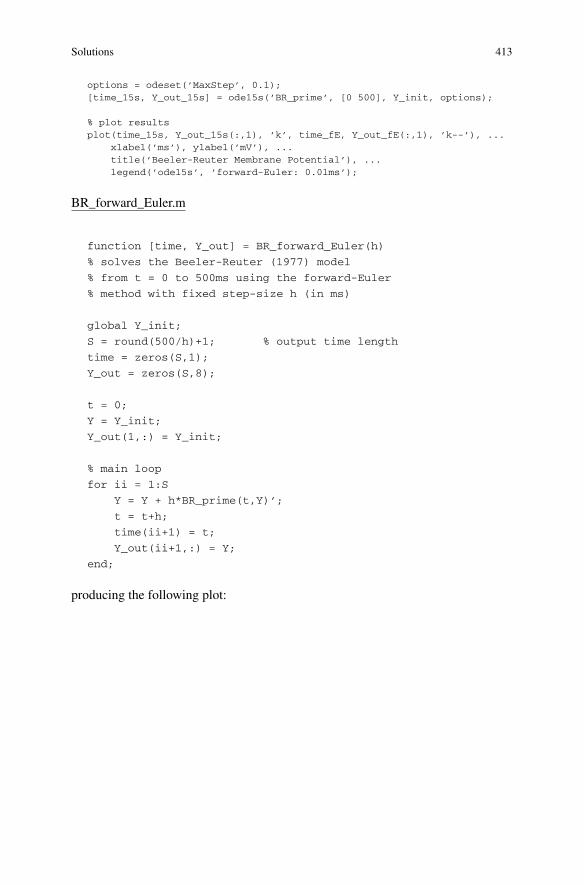
Solutions 413

options = odeset(’MaxStep’, 0.1);[time_15s, Y_out_15s] = ode15s(’BR_prime’, [0 500], Y_init, options);

% plot resultsplot(time_15s, Y_out_15s(:,1), ’k’, time_fE, Y_out_fE(:,1), ’k--’), ...

xlabel(’ms’), ylabel(’mV’), ...title(’Beeler-Reuter Membrane Potential’), ...legend(’ode15s’, ’forward-Euler: 0.01ms’);

BR_forward_Euler.m

function [time, Y_out] = BR_forward_Euler(h)

% solves the Beeler-Reuter (1977) model

% from t = 0 to 500ms using the forward-Euler

% method with fixed step-size h (in ms)

global Y_init;

S = round(500/h)+1; % output time length

time = zeros(S,1);

Y_out = zeros(S,8);

t = 0;

Y = Y_init;

Y_out(1,:) = Y_init;

% main loop

for ii = 1:S

Y = Y + h*BR_prime(t,Y)’;

t = t+h;

time(ii+1) = t;

Y_out(ii+1,:) = Y;

end;

producing the following plot:

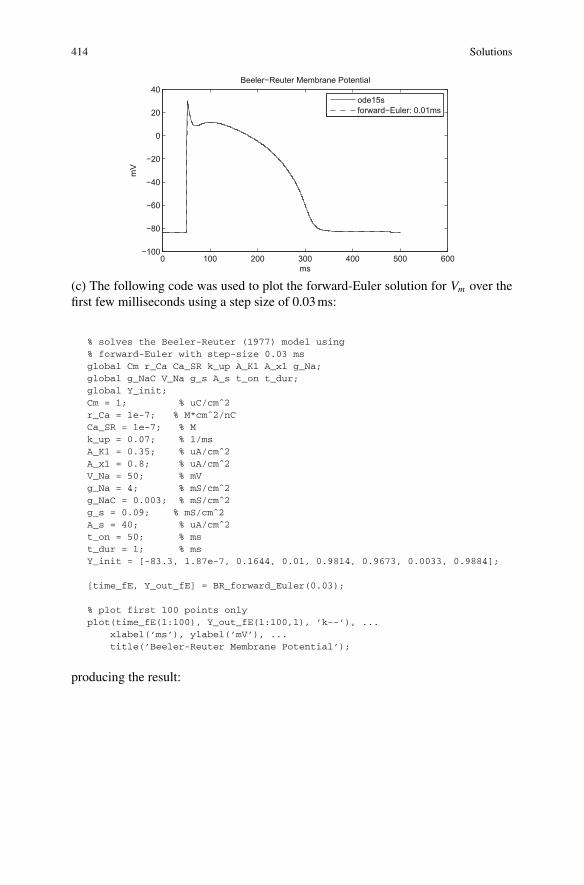
414 Solutions

0 100 200 300 400 500 600−100

−80

−60

−40

−20

0

20

40

ms

mV


ode15sforward−Euler: 0.01ms

(c) The following code was used to plot the forward-Euler solution for Vm over thefirst few milliseconds using a step size of 0.03ms:

% solves the Beeler-Reuter (1977) model using% forward-Euler with step-size 0.03 msglobal Cm r_Ca Ca_SR k_up A_K1 A_x1 g_Na;global g_NaC V_Na g_s A_s t_on t_dur;global Y_init;Cm = 1; % uC/cmˆ2r_Ca = 1e-7; % M*cmˆ2/nCCa_SR = 1e-7; % Mk_up = 0.07; % 1/msA_K1 = 0.35; % uA/cmˆ2A_x1 = 0.8; % uA/cmˆ2V_Na = 50; % mVg_Na = 4; % mS/cmˆ2g_NaC = 0.003; % mS/cmˆ2g_s = 0.09; % mS/cmˆ2A_s = 40; % uA/cmˆ2t_on = 50; % mst_dur = 1; % msY_init = [-83.3, 1.87e-7, 0.1644, 0.01, 0.9814, 0.9673, 0.0033, 0.9884];

[time_fE, Y_out_fE] = BR_forward_Euler(0.03);

% plot first 100 points onlyplot(time_fE(1:100), Y_out_fE(1:100,1), ’k--’), ...

xlabel(’ms’), ylabel(’mV’), ...title(’Beeler-Reuter Membrane Potential’);

producing the result:

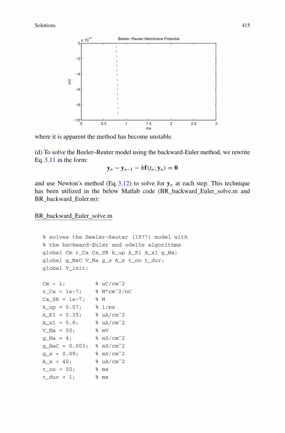
Solutions 415

0 0.5 1 1.5 2 2.5 3−10

−8

−6

−4

−2

0x 1010

ms

mV


where it is apparent the method has become unstable.

(d) To solve the Beeler–Reuter model using the backward-Euler method, we rewriteEq.3.11 in the form:

yn − yn−1 − hf(tn, yn) = 0

and use Newton’s method (Eq.3.12) to solve for yn at each step. This techniquehas been utilized in the below Matlab code (BR_backward_Euler_solve.m andBR_backward_Euler.m):

BR_backward_Euler_solve.m

% solves the Beeler-Reuter (1977) model with

% the backward-Euler and ode15s algorithms

global Cm r_Ca Ca_SR k_up A_K1 A_x1 g_Na;

global g_NaC V_Na g_s A_s t_on t_dur;

global Y_init;

Cm = 1; % uC/cmˆ2

r_Ca = 1e-7; % M*cmˆ2/nC

Ca_SR = 1e-7; % M

k_up = 0.07; % 1/ms

A_K1 = 0.35; % uA/cmˆ2

A_x1 = 0.8; % uA/cmˆ2

V_Na = 50; % mV

g_Na = 4; % mS/cmˆ2

g_NaC = 0.003; % mS/cmˆ2

g_s = 0.09; % mS/cmˆ2

A_s = 40; % uA/cmˆ2

t_on = 50; % ms

t_dur = 1; % ms

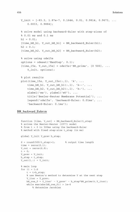
http://dx.doi.org/10.1007/978-3-642-54801-7_3

http://dx.doi.org/10.1007/978-3-642-54801-7_3

416 Solutions

Y_init = [-83.3, 1.87e-7, 0.1644, 0.01, 0.9814, 0.9673, ...

0.0033, 0.9884];

% solve model using backward-Euler with step-sizes of

% 0.01 ms and 0.1 ms

h1 = 0.01;

[time_bE_h1, Y_out_bE_h1] = BR_backward_Euler(h1);

h2 = 0.1;

[time_bE_h2, Y_out_bE_h2] = BR_backward_Euler(h2);


options = odeset(’MaxStep’, 0.1);

[time_15s, Y_out_15s] = ode15s(’BR_prime’, [0 500], ...

Y_init, options);

% plot results

plot(time_15s, Y_out_15s(:,1), ’k’, ...

time_bE_h1, Y_out_bE_h1(:,1), ’k--’, ...

time_bE_h2, Y_out_bE_h2(:,1), ’k:’), ...

xlabel(’ms’), ylabel(’mV’), ...

title(’Beeler-Reuter Membrane Potential’), ...

legend(’ode15s’, ’backward-Euler: 0.01ms’, ...

’backward-Euler: 0.1ms’);

BR_backward_Euler.m

function [time, Y_out] = BR_backward_Euler(t_step)% solves the Beeler-Reuter (1977) model% from t = 0 to 500ms using the backward-Euler% method with fixed step-size t_step (in ms)

global Y_init Y_prev h_step;

S = round(500/t_step)+1; % output time lengthtime = zeros(S,1);Y_out = zeros(S,8);t = 0;Y_prev = Y_init;h_step = t_step;Y_out(1,:) = Y_init;

% main loopfor ii = 1:S

t = t+h_step;% use Newton’s method to determine Y at the next stepY_iter = Y_prev;bE_res_0 = Y_iter’ - Y_prev’ - h_step*BR_prime(t,Y_iter);while max(abs(bE_res_0)) > 1e-6

% determine Jacobian

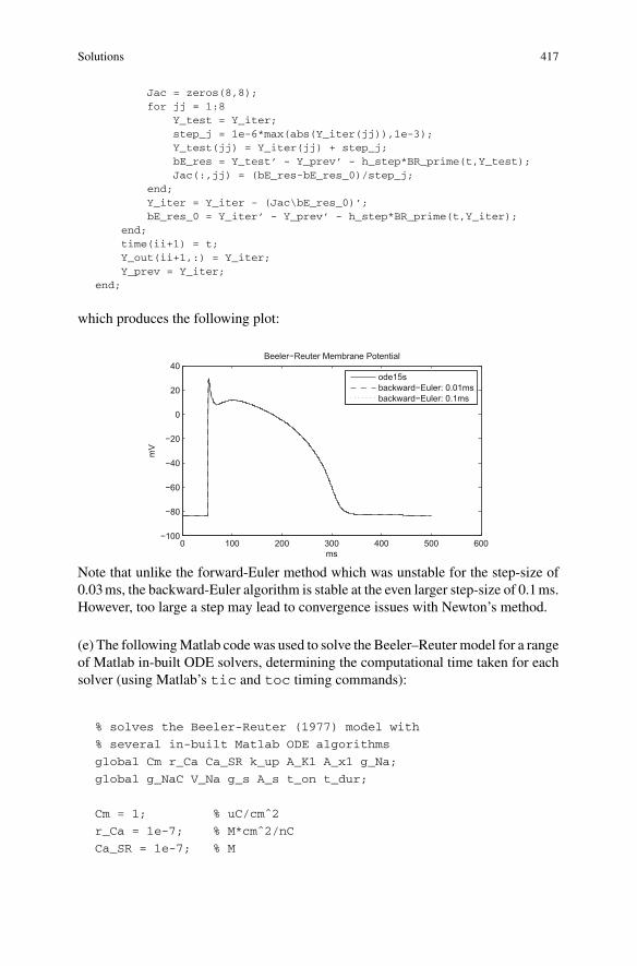
Solutions 417

Jac = zeros(8,8);for jj = 1:8

Y_test = Y_iter;step_j = 1e-6*max(abs(Y_iter(jj)),1e-3);Y_test(jj) = Y_iter(jj) + step_j;bE_res = Y_test’ - Y_prev’ - h_step*BR_prime(t,Y_test);Jac(:,jj) = (bE_res-bE_res_0)/step_j;

end;Y_iter = Y_iter - (Jac\bE_res_0)’;bE_res_0 = Y_iter’ - Y_prev’ - h_step*BR_prime(t,Y_iter);

end;time(ii+1) = t;Y_out(ii+1,:) = Y_iter;Y_prev = Y_iter;

end;

which produces the following plot:

0 100 200 300 400 500 600−100

−80

−60

−40

−20

0

20

40

ms

mV


ode15sbackward−Euler: 0.01msbackward−Euler: 0.1ms

Note that unlike the forward-Euler method which was unstable for the step-size of0.03ms, the backward-Euler algorithm is stable at the even larger step-size of 0.1ms.However, too large a step may lead to convergence issues with Newton’s method.

(e) The followingMatlab code was used to solve the Beeler–Reuter model for a rangeof Matlab in-built ODE solvers, determining the computational time taken for eachsolver (using Matlab’s tic and toc timing commands):

% solves the Beeler-Reuter (1977) model with

% several in-built Matlab ODE algorithms

global Cm r_Ca Ca_SR k_up A_K1 A_x1 g_Na;

global g_NaC V_Na g_s A_s t_on t_dur;

Cm = 1; % uC/cmˆ2

r_Ca = 1e-7; % M*cmˆ2/nC

Ca_SR = 1e-7; % M

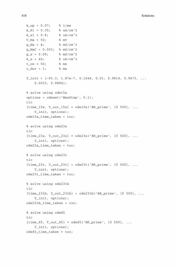
418 Solutions

k_up = 0.07; % 1/ms

A_K1 = 0.35; % uA/cmˆ2

A_x1 = 0.8; % uA/cmˆ2

V_Na = 50; % mV


g_NaC = 0.003; % mS/cmˆ2

g_s = 0.09; % mS/cmˆ2

A_s = 40; % uA/cmˆ2

t_on = 50; % ms

t_dur = 1; % ms

Y_init = [-83.3, 1.87e-7, 0.1644, 0.01, 0.9814, 0.9673, ...

0.0033, 0.9884];


options = odeset(’MaxStep’, 0.1);

tic


Y_init, options);

ode15s_time_taken = toc;


tic


Y_init, options);

ode23s_time_taken = toc;

% solve using ode23t

tic

[time_23t, Y_out_23t] = ode23t(’BR_prime’, [0 500], ...

Y_init, options);

ode23t_time_taken = toc;

% solve using ode23tb

tic

[time_23tb, Y_out_23tb] = ode23tb(’BR_prime’, [0 500], ...

Y_init, options);

ode23tb_time_taken = toc;

% solve using ode45

tic

[time_45, Y_out_45] = ode45(’BR_prime’, [0 500], ...

Y_init, options);

ode45_time_taken = toc;

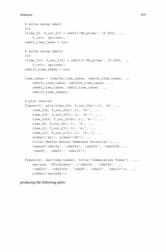
Solutions 419

% solve using ode23

tic


Y_init, options);


% solve using ode113

tic


Y_init, options);


time_taken = [ode15s_time_taken, ode23s_time_taken, ...

ode23t_time_taken, ode23tb_time_taken, ...

ode45_time_taken, ode23_time_taken, ...

ode113_time_taken];

% plot results

figure(1), plot(time_15s, Y_out_15s(:,1), ’b’, ...

time_23s, Y_out_23s(:,1), ’b:’, ...

time_23t, Y_out_23t(:,1), ’b-.’, ...

time_23tb, Y_out_23tb(:,1), ’b--’, ...

time_45, Y_out_45(:,1), ’k’, ...

time_23, Y_out_23(:,1), ’k:’, ...

time_113, Y_out_113(:,1), ’k-.’), ...


title(’Beeler-Reuter Membrane Potential’), ...

legend(’ode15s’, ’ode23s’, ’ode23t’, ’ode23tb’,...

’ode45’, ’ode23’, ’ode113’);

figure(2), bar(time_taken), title(’Computation Times’), ...

set(gca, ’XTickLabel’, {’ode15s’, ’ode23s’, ...

’ode23t’, ’ode23tb’, ’ode45’, ’ode23’, ’ode113’}), ...

ylabel(’seconds’);

producing the following plots:

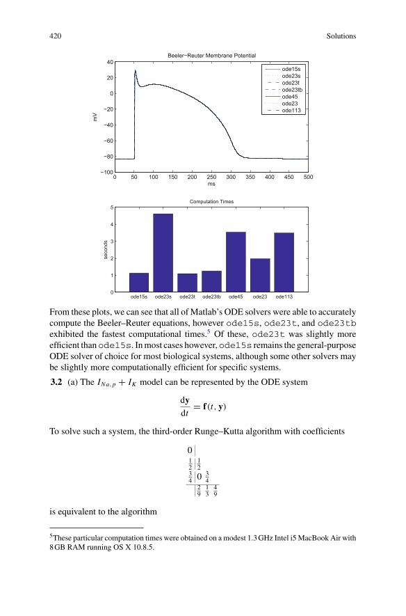
420 Solutions

0 50 100 150 200 250 300 350 400 450 500−100

−80

−60

−40

−20

0

20

40

ms

mV


ode15sode23sode23tode23tbode45ode23ode113

ode15s ode23s ode23t ode23tb ode45 ode23 ode1130

1

2

3

4

5Computation Times

seco

nds

From these plots, we can see that all of Matlab’s ODE solvers were able to accuratelycompute the Beeler–Reuter equations, however ode15s, ode23t, and ode23tbexhibited the fastest computational times.5 Of these, ode23t was slightly moreefficient thanode15s. Inmost cases however,ode15s remains the general-purposeODE solver of choice for most biological systems, although some other solvers maybe slightly more computationally efficient for specific systems.

3.2 (a) The INa,p + IK model can be represented by the ODE system

dydt

= f(t, y)

To solve such a system, the third-order Runge–Kutta algorithm with coefficients

012

12

34 0 3

429

13

49

is equivalent to the algorithm

5These particular computation times were obtained on a modest 1.3GHz Intel i5MacBook Air with8GB RAM running OS X 10.8.5.

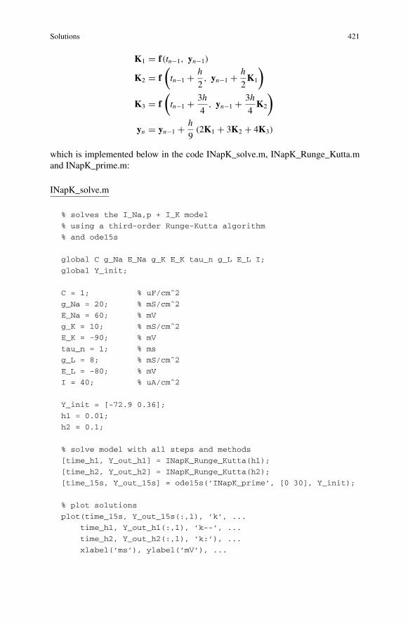
Solutions 421

K1 = f(tn−1, yn−1)

K2 = f(tn−1 + h

2, yn−1 + h

2K1

)

K3 = f(tn−1 + 3h

4, yn−1 + 3h

4K2

)

yn = yn−1 + h

9(2K1 + 3K2 + 4K3)

which is implemented below in the code INapK_solve.m, INapK_Runge_Kutta.mand INapK_prime.m:

INapK_solve.m

% solves the I_Na,p + I_K model

% using a third-order Runge-Kutta algorithm

% and ode15s

global C g_Na E_Na g_K E_K tau_n g_L E_L I;

global Y_init;

C = 1; % uF/cmˆ2


E_Na = 60; % mV

g_K = 10; % mS/cmˆ2

E_K = -90; % mV

tau_n = 1; % ms

g_L = 8; % mS/cmˆ2

E_L = -80; % mV

I = 40; % uA/cmˆ2

Y_init = [-72.9 0.36];

h1 = 0.01;

h2 = 0.1;

% solve model with all steps and methods

[time_h1, Y_out_h1] = INapK_Runge_Kutta(h1);

[time_h2, Y_out_h2] = INapK_Runge_Kutta(h2);

[time_15s, Y_out_15s] = ode15s(’INapK_prime’, [0 30], Y_init);

% plot solutions


time_h1, Y_out_h1(:,1), ’k--’, ...

time_h2, Y_out_h2(:,1), ’k:’), ...


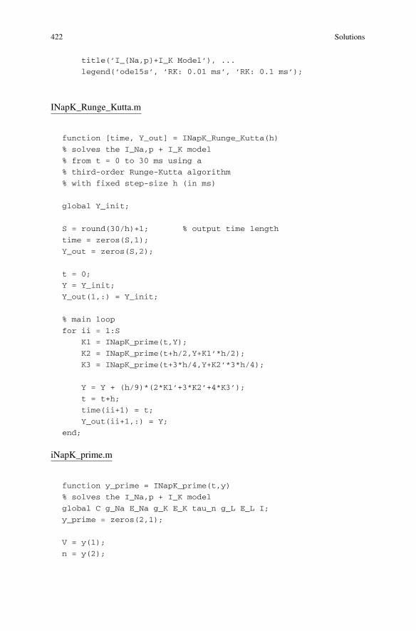
422 Solutions

title(’I_{Na,p}+I_K Model’), ...

legend(’ode15s’, ’RK: 0.01 ms’, ’RK: 0.1 ms’);

INapK_Runge_Kutta.m

function [time, Y_out] = INapK_Runge_Kutta(h)


% from t = 0 to 30 ms using a

% third-order Runge-Kutta algorithm

% with fixed step-size h (in ms)

global Y_init;

S = round(30/h)+1; % output time length

time = zeros(S,1);

Y_out = zeros(S,2);

t = 0;

Y = Y_init;

Y_out(1,:) = Y_init;

% main loop

for ii = 1:S

K1 = INapK_prime(t,Y);

K2 = INapK_prime(t+h/2,Y+K1’*h/2);

K3 = INapK_prime(t+3*h/4,Y+K2’*3*h/4);

Y = Y + (h/9)*(2*K1’+3*K2’+4*K3’);

t = t+h;

time(ii+1) = t;

Y_out(ii+1,:) = Y;

end;

iNapK_prime.m

function y_prime = INapK_prime(t,y)




V = y(1);

n = y(2);

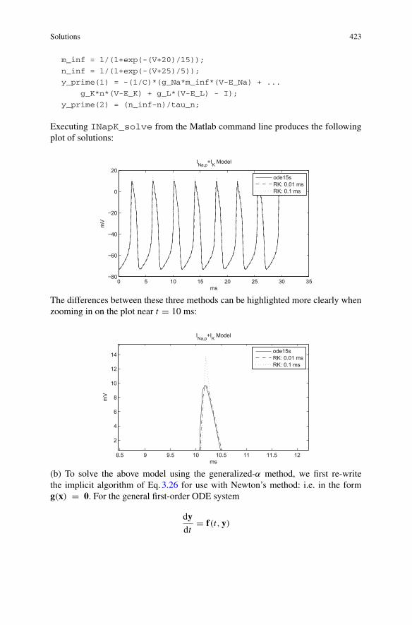
Solutions 423

m_inf = 1/(1+exp(-(V+20)/15));

n_inf = 1/(1+exp(-(V+25)/5));

y_prime(1) = -(1/C)*(g_Na*m_inf*(V-E_Na) + ...

g_K*n*(V-E_K) + g_L*(V-E_L) - I);

y_prime(2) = (n_inf-n)/tau_n;

Executing INapK_solve from the Matlab command line produces the followingplot of solutions:

0 5 10 15 20 25 30 35−80

−60

−40

−20

0

20

ms

mV

INa,p+IK Model

ode15sRK: 0.01 msRK: 0.1 ms

The differences between these three methods can be highlighted more clearly whenzooming in on the plot near t = 10 ms:

8.5 9 9.5 10 10.5 11 11.5 12

2

4

6

8

10

12

14

ms

mV

INa,p+IK Model

ode15sRK: 0.01 msRK: 0.1 ms

(b) To solve the above model using the generalized-α method, we first re-writethe implicit algorithm of Eq.3.26 for use with Newton’s method: i.e. in the formg(x) = 0. For the general first-order ODE system

dydt

= f(t, y)

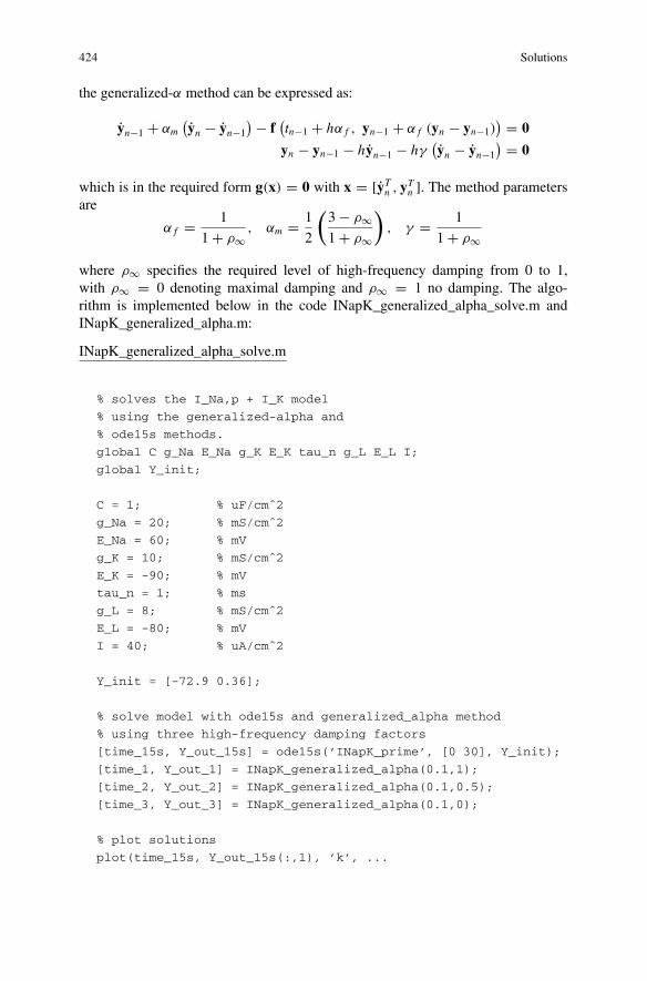
http://dx.doi.org/10.1007/978-3-642-54801-7_3

424 Solutions

the generalized-α method can be expressed as:

yn−1 + αm(yn − yn−1

) − f(tn−1 + hα f , yn−1 + α f (yn − yn−1)

) = 0

yn − yn−1 − hyn−1 − hγ(yn − yn−1

) = 0

which is in the required form g(x) = 0 with x = [yTn , yTn ]. The method parametersare

α f = 1

1 + ρ∞, αm = 1

2

(3 − ρ∞1 + ρ∞

), γ = 1

1 + ρ∞

where ρ∞ specifies the required level of high-frequency damping from 0 to 1,with ρ∞ = 0 denoting maximal damping and ρ∞ = 1 no damping. The algo-rithm is implemented below in the code INapK_generalized_alpha_solve.m andINapK_generalized_alpha.m:

INapK_generalized_alpha_solve.m


% using the generalized-alpha and

% ode15s methods.


global Y_init;

C = 1; % uF/cmˆ2


E_Na = 60; % mV

g_K = 10; % mS/cmˆ2

E_K = -90; % mV

tau_n = 1; % ms

g_L = 8; % mS/cmˆ2

E_L = -80; % mV

I = 40; % uA/cmˆ2

Y_init = [-72.9 0.36];

% solve model with ode15s and generalized_alpha method

% using three high-frequency damping factors

[time_15s, Y_out_15s] = ode15s(’INapK_prime’, [0 30], Y_init);

[time_1, Y_out_1] = INapK_generalized_alpha(0.1,1);

[time_2, Y_out_2] = INapK_generalized_alpha(0.1,0.5);

[time_3, Y_out_3] = INapK_generalized_alpha(0.1,0);

% plot solutions


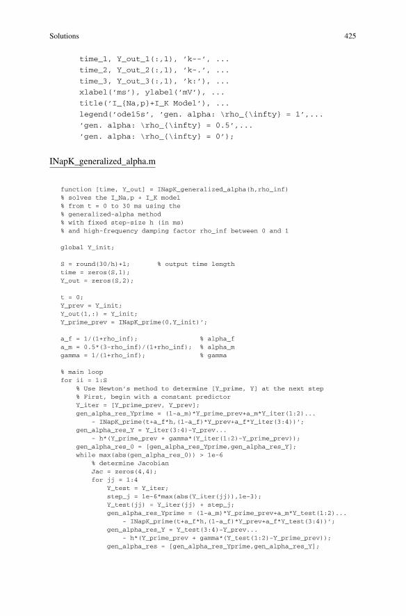
Solutions 425

time_1, Y_out_1(:,1), ’k--’, ...

time_2, Y_out_2(:,1), ’k-.’, ...

time_3, Y_out_3(:,1), ’k:’), ...


title(’I_{Na,p}+I_K Model’), ...

legend(’ode15s’, ’gen. alpha: \rho_{\infty} = 1’,...

’gen. alpha: \rho_{\infty} = 0.5’,...

’gen. alpha: \rho_{\infty} = 0’);

INapK_generalized_alpha.m

function [time, Y_out] = INapK_generalized_alpha(h,rho_inf)% solves the I_Na,p + I_K model% from t = 0 to 30 ms using the% generalized-alpha method% with fixed step-size h (in ms)% and high-frequency damping factor rho_inf between 0 and 1

global Y_init;

S = round(30/h)+1; % output time lengthtime = zeros(S,1);Y_out = zeros(S,2);

t = 0;Y_prev = Y_init;Y_out(1,:) = Y_init;Y_prime_prev = INapK_prime(0,Y_init)’;

a_f = 1/(1+rho_inf); % alpha_fa_m = 0.5*(3-rho_inf)/(1+rho_inf); % alpha_mgamma = 1/(1+rho_inf); % gamma

% main loopfor ii = 1:S

% Use Newton’s method to determine [Y_prime, Y] at the next step% First, begin with a constant predictorY_iter = [Y_prime_prev, Y_prev];gen_alpha_res_Yprime = (1-a_m)*Y_prime_prev+a_m*Y_iter(1:2)...

- INapK_prime(t+a_f*h,(1-a_f)*Y_prev+a_f*Y_iter(3:4))’;gen_alpha_res_Y = Y_iter(3:4)-Y_prev...

- h*(Y_prime_prev + gamma*(Y_iter(1:2)-Y_prime_prev));gen_alpha_res_0 = [gen_alpha_res_Yprime,gen_alpha_res_Y];while max(abs(gen_alpha_res_0)) > 1e-6

% determine JacobianJac = zeros(4,4);for jj = 1:4

Y_test = Y_iter;step_j = 1e-6*max(abs(Y_iter(jj)),1e-3);Y_test(jj) = Y_iter(jj) + step_j;gen_alpha_res_Yprime = (1-a_m)*Y_prime_prev+a_m*Y_test(1:2)...

- INapK_prime(t+a_f*h,(1-a_f)*Y_prev+a_f*Y_test(3:4))’;gen_alpha_res_Y = Y_test(3:4)-Y_prev...

- h*(Y_prime_prev + gamma*(Y_test(1:2)-Y_prime_prev));gen_alpha_res = [gen_alpha_res_Yprime,gen_alpha_res_Y];

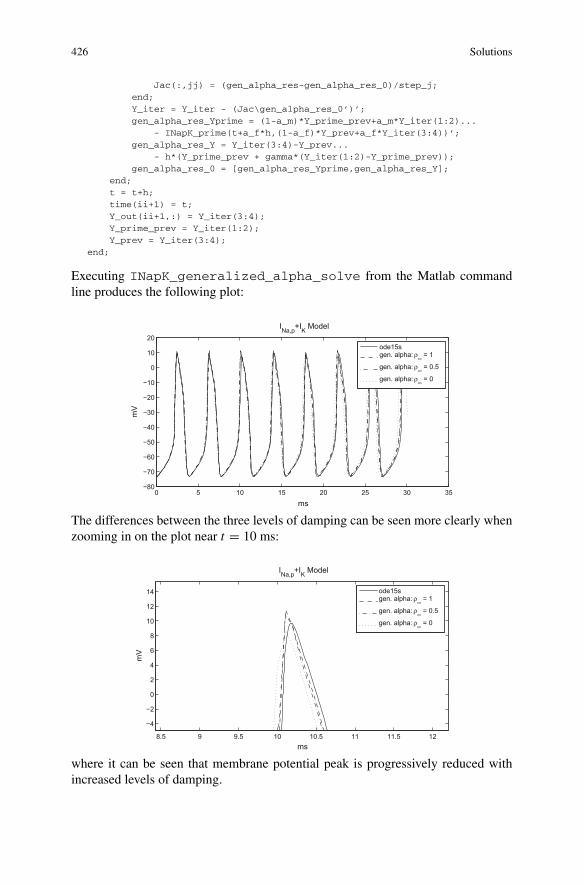
426 Solutions

Jac(:,jj) = (gen_alpha_res-gen_alpha_res_0)/step_j;end;Y_iter = Y_iter - (Jac\gen_alpha_res_0’)’;gen_alpha_res_Yprime = (1-a_m)*Y_prime_prev+a_m*Y_iter(1:2)...

- INapK_prime(t+a_f*h,(1-a_f)*Y_prev+a_f*Y_iter(3:4))’;gen_alpha_res_Y = Y_iter(3:4)-Y_prev...

- h*(Y_prime_prev + gamma*(Y_iter(1:2)-Y_prime_prev));gen_alpha_res_0 = [gen_alpha_res_Yprime,gen_alpha_res_Y];

end;t = t+h;time(ii+1) = t;Y_out(ii+1,:) = Y_iter(3:4);Y_prime_prev = Y_iter(1:2);Y_prev = Y_iter(3:4);

end;

Executing INapK_generalized_alpha_solve from the Matlab commandline produces the following plot:

0 5 10 15 20 25 30 35−80

−70

−60

−50

−40

−30

−20

−10

0

10

20

ms

mV

INa,p+IK Model

ode15sgen. alpha: ρ∞ = 1

gen. alpha: ρ∞ = 0.5

gen. alpha: ρ∞ = 0

The differences between the three levels of damping can be seen more clearly whenzooming in on the plot near t = 10 ms:

8.5 9 9.5 10 10.5 11 11.5 12

−4

−2

0

2

4

6

8

10

12

14

ms

mV

INa,p+IK Model

ode15sgen. alpha: ρ∞ = 1

gen. alpha: ρ∞ = 0.5

gen. alpha: ρ∞ = 0

where it can be seen that membrane potential peak is progressively reduced withincreased levels of damping.

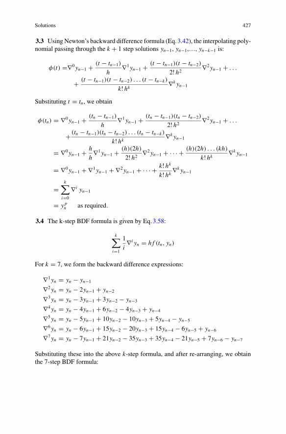
Solutions 427

3.3 Using Newton’s backward difference formula (Eq. 3.42), the interpolating poly-nomial passing through the k + 1 step solutions yn−1, yn−1,…, yn−k−1 is:

φ(t) =∇0yn−1 + (t − tn−1)

h∇1yn−1 + (t − tn−1)(t − tn−2)

2! h2 ∇2yn−1 + . . .

+ (t − tn−1)(t − tn−2) . . . (t − tn−k)

k! hk ∇k yn−1

Substituting t = tn , we obtain

φ(tn) = ∇0yn−1 + (tn − tn−1)

h∇1yn−1 + (tn − tn−1)(tn − tn−2)

2! h2 ∇2yn−1 + . . .

+ (tn − tn−1)(tn − tn−2) . . . (tn − tn−k)

k! hk ∇k yn−1

= ∇0yn−1 + h

h∇1yn−1 + (h)(2h)

2! h2 ∇2yn−1 + · · · + (h)(2h) . . . (kh)

k! hk ∇k yn−1

= ∇0yn−1 + ∇1yn−1 + ∇2yn−1 + · · · + k! hkk! hk ∇k yn−1

=k∑

i=0

∇ i yn−1

= y pn as required.

3.4 The k-step BDF formula is given by Eq.3.58:

k∑i=1

1

i∇ i yn = h f (tn, yn)

For k = 7, we form the backward difference expressions:

∇1yn = yn − yn−1

∇2yn = yn − 2yn−1 + yn−2

∇3yn = yn − 3yn−1 + 3yn−2 − yn−3

∇4yn = yn − 4yn−1 + 6yn−2 − 4yn−3 + yn−4

∇5yn = yn − 5yn−1 + 10yn−2 − 10yn−3 + 5yn−4 − yn−5

∇6yn = yn − 6yn−1 + 15yn−2 − 20yn−3 + 15yn−4 − 6yn−5 + yn−6

∇7yn = yn − 7yn−1 + 21yn−2 − 35yn−3 + 35yn−4 − 21yn−5 + 7yn−6 − yn−7

Substituting these into the above k-step formula, and after re-arranging, we obtainthe 7-step BDF formula:

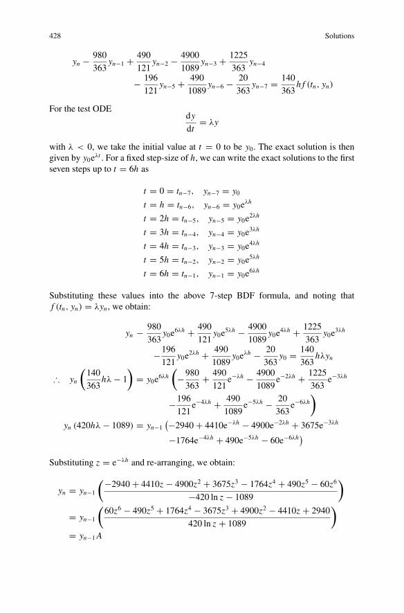
http://dx.doi.org/10.1007/978-3-642-54801-7_3

http://dx.doi.org/10.1007/978-3-642-54801-7_3

428 Solutions

yn − 980

363yn−1 + 490

121yn−2 − 4900

1089yn−3 + 1225

363yn−4

− 196

121yn−5 + 490

1089yn−6 − 20

363yn−7 = 140

363h f (tn, yn)

For the test ODEdy

dt= λy

with λ < 0, we take the initial value at t = 0 to be y0. The exact solution is thengiven by y0eλt . For a fixed step-size of h, we can write the exact solutions to the firstseven steps up to t = 6h as

t = 0 = tn−7, yn−7 = y0t = h = tn−6, yn−6 = y0e

λh

t = 2h = tn−5, yn−5 = y0e2λh

t = 3h = tn−4, yn−4 = y0e3λh

t = 4h = tn−3, yn−3 = y0e4λh

t = 5h = tn−2, yn−2 = y0e5λh

t = 6h = tn−1, yn−1 = y0e6λh

Substituting these values into the above 7-step BDF formula, and noting thatf (tn, yn) = λyn , we obtain:

yn − 980

363y0e

6λh + 490

121y0e

5λh − 4900

1089y0e

4λh + 1225

363y0e

3λh

−196

121y0e

2λh + 490

1089y0e

λh − 20

363y0 = 140

363hλyn

∴ yn

(140

363hλ − 1

)= y0e

6λh

(−980

363+ 490

121e−λh − 4900

1089e−2λh + 1225

363e−3λh

−196

121e−4λh + 490

1089e−5λh − 20

363e−6λh

)

yn (420hλ − 1089) = yn−1(−2940 + 4410e−λh − 4900e−2λh + 3675e−3λh

−1764e−4λh + 490e−5λh − 60e−6λh)

Substituting z = e−λh and re-arranging, we obtain:

yn = yn−1

(−2940 + 4410z − 4900z2 + 3675z3 − 1764z4 + 490z5 − 60z6

−420 ln z − 1089

)

= yn−1

(60z6 − 490z5 + 1764z4 − 3675z3 + 4900z2 − 4410z + 2940

420 ln z + 1089

)

= yn−1A

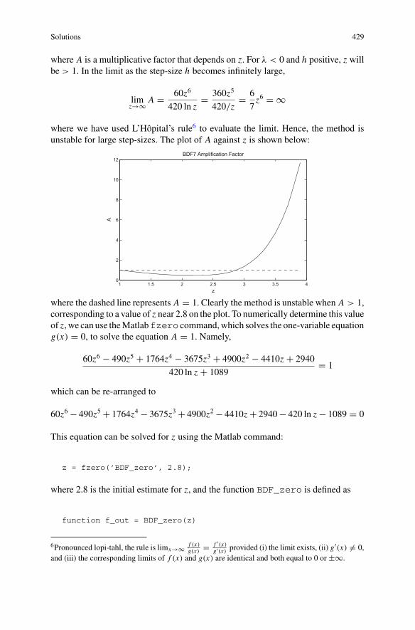
Solutions 429

where A is a multiplicative factor that depends on z. For λ < 0 and h positive, z willbe > 1. In the limit as the step-size h becomes infinitely large,

limz→∞ A = 60z6

420 ln z= 360z5

420/z= 6

7z6 = ∞

where we have used L’Hôpital’s rule6 to evaluate the limit. Hence, the method isunstable for large step-sizes. The plot of A against z is shown below:

1 1.5 2 2.5 3 3.5 40

2

4

6

8

10

12

z

A

BDF7 Amplification Factor

where the dashed line represents A = 1. Clearly the method is unstable when A > 1,corresponding to a value of z near 2.8 on the plot. To numerically determine this valueof z, we can use theMatlabfzero command,which solves the one-variable equationg(x) = 0, to solve the equation A = 1. Namely,

60z6 − 490z5 + 1764z4 − 3675z3 + 4900z2 − 4410z + 2940

420 ln z + 1089= 1

which can be re-arranged to

60z6 − 490z5 + 1764z4 − 3675z3 + 4900z2 − 4410z + 2940− 420 ln z − 1089 = 0

This equation can be solved for z using the Matlab command:

z = fzero(’BDF_zero’, 2.8);

where 2.8 is the initial estimate for z, and the function BDF_zero is defined as

function f_out = BDF_zero(z)

6Pronounced lopi-tahl, the rule is limx→∞ f (x)g(x) = f ′(x)

g′(x) provided (i) the limit exists, (ii) g′(x) �= 0,and (iii) the corresponding limits of f (x) and g(x) are identical and both equal to 0 or ±∞.

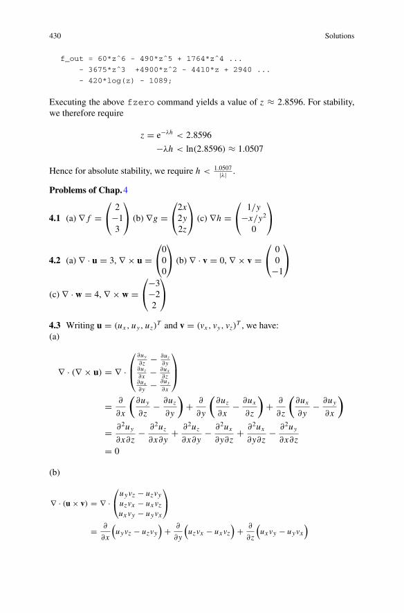
430 Solutions

f_out = 60*zˆ6 - 490*zˆ5 + 1764*zˆ4 ...

- 3675*zˆ3 +4900*zˆ2 - 4410*z + 2940 ...

- 420*log(z) - 1089;

Executing the above fzero command yields a value of z ≈ 2.8596. For stability,we therefore require

z = e−λh < 2.8596

−λh < ln(2.8596) ≈ 1.0507

Hence for absolute stability, we require h < 1.0507|λ| .

Problems of Chap.4

4.1 (a) ∇ f =⎛⎝ 2

−13

⎞⎠ (b) ∇g =

⎛⎝2x2y2z

⎞⎠ (c) ∇h =

⎛⎝ 1/y

−x/y2

0

⎞⎠

4.2 (a) ∇ · u = 3, ∇ × u =⎛⎝000

⎞⎠ (b) ∇ · v = 0, ∇ × v =

⎛⎝ 0

0−1

⎞⎠

(c) ∇ · w = 4, ∇ × w =⎛⎝−3

−22

⎞⎠

4.3 Writing u = (ux , uy, uz)T and v = (vx , vy, vz)T , we have:

(a)

∇ · (∇ × u) = ∇ ·⎛⎜⎝

∂uy

∂z − ∂uz∂y

∂uz∂x − ∂ux

∂z∂ux∂y − ∂uy

∂x

⎞⎟⎠

= ∂

∂x

(∂uy

∂z− ∂uz

∂y

)+ ∂

∂y

(∂uz

∂x− ∂ux

∂z

)+ ∂

∂z

(∂ux

∂y− ∂uy

∂x

)

= ∂2uy

∂x∂z− ∂2uz

∂x∂y+ ∂2uz

∂x∂y− ∂2ux

∂y∂z+ ∂2ux

∂y∂z− ∂2uy

∂x∂z= 0

(b)

∇ · (u × v) = ∇ ·⎛⎝uyvz − uzvyuzvx − uxvzux vy − uyvx

⎞⎠

= ∂

∂x

(uyvz − uzvy

)+ ∂

∂y

(uzvx − uxvz

)+ ∂

∂z

(uxvy − uyvx

)

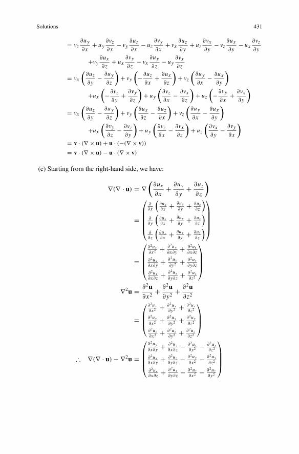
http://dx.doi.org/10.1007/978-3-642-54801-7_4

Solutions 431

= vz∂uy∂x

+ uy∂vz∂x

− vy∂uz∂x

− uz∂vy∂x

+ vx∂uz∂y

+ uz∂vx∂y

− vz∂ux∂y

− ux∂vz∂y

+vy∂ux∂z

+ ux∂vy∂z

− vx∂uy∂z

− uy∂vx∂z

= vx

(∂uz∂y

− ∂uy∂z

)+ vy

(−∂uz

∂x+ ∂ux

∂z

)+ vz

(∂uy∂x

− ∂ux∂y

)

+ux

(−∂vz

∂y+ ∂vy

∂z

)+ uy

(∂vz∂x

− ∂vx∂z

)+ uz

(−∂vy

∂x+ ∂vx

∂y

)

= vx

(∂uz∂y

− ∂uy∂z

)+ vy

(∂ux∂z

− ∂uz∂x

)+ vz

(∂uy∂x

− ∂ux∂y

)

+ux

(∂vy∂z

− ∂vz∂y

)+ uy

(∂vz∂x

− ∂vx∂z

)+ uz

(∂vx∂y

− ∂vy∂x

)

= v · (∇ × u) + u · (−(∇ × v))

= v · (∇ × u) − u · (∇ × v)

(c) Starting from the right-hand side, we have:

∇(∇ · u) = ∇(

∂ux

∂x+ ∂uy

∂y+ ∂uz

∂z

)

=

⎛⎜⎜⎜⎜⎝

∂∂x

(∂ux∂x + ∂uy

∂y + ∂uz∂z

)∂∂y

(∂ux∂x + ∂uy

∂y + ∂uz∂z

)∂∂z

(∂ux∂x + ∂uy

∂y + ∂uz∂z

)

⎞⎟⎟⎟⎟⎠

=

⎛⎜⎜⎜⎝

∂2ux∂x2 + ∂2uy

∂x∂y + ∂2uz∂x∂z

∂2ux∂x∂y + ∂2uy

∂y2 + ∂2uz∂y∂z

∂2ux∂x∂z + ∂2uy

∂y∂z + ∂2uz∂z2

⎞⎟⎟⎟⎠

∇2u = ∂2u∂x2

+ ∂2u∂y2

+ ∂2u∂z2

=

⎛⎜⎜⎝

∂2ux∂x2 + ∂2ux

∂y2 + ∂2ux∂z2

∂2uy

∂x2 + ∂2uy

∂y2 + ∂2uy

∂z2

∂2uz∂x2 + ∂2uz

∂y2 + ∂2uz∂z2

⎞⎟⎟⎠

∴ ∇(∇ · u) − ∇2u =

⎛⎜⎜⎜⎝

∂2uy

∂x∂y + ∂2uz∂x∂z − ∂2ux

∂y2 − ∂2ux∂z2

∂2ux∂x∂y + ∂2uz

∂y∂z − ∂2uy

∂x2 − ∂2uy

∂z2


∂y∂z − ∂2uz∂x2 − ∂2uz

∂y2

⎞⎟⎟⎟⎠

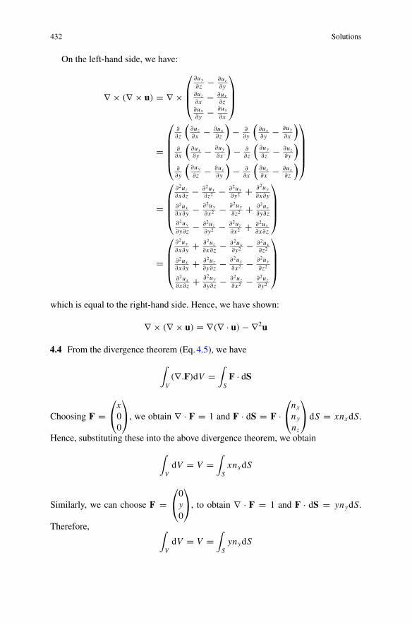
432 Solutions

On the left-hand side, we have:

∇ × (∇ × u) = ∇ ×

⎛⎜⎜⎝

∂uy

∂z − ∂uz∂y

∂uz∂x − ∂ux

∂z∂ux∂y − ∂uy

∂x

⎞⎟⎟⎠

=

⎛⎜⎜⎜⎜⎝

∂∂z

(∂uz∂x − ∂ux

∂z

)− ∂

∂y

(∂ux∂y − ∂uy

∂x

)∂∂x

(∂ux∂y − ∂uy

∂x

)− ∂

∂z

(∂uy

∂z − ∂uz∂y

)∂∂y

(∂uy

∂z − ∂uz∂y

)− ∂

∂x

(∂uz∂x − ∂ux

∂z

)

⎞⎟⎟⎟⎟⎠

=

⎛⎜⎜⎜⎝

∂2uz∂x∂z − ∂2ux

∂z2 − ∂2ux∂y2 + ∂2uy

∂x∂y

∂2ux∂x∂y − ∂2uy

∂x2 − ∂2uy

∂z2 + ∂2uz∂y∂z

∂2uy

∂y∂z − ∂2uz∂y2 − ∂2uz

∂x2 + ∂2ux∂x∂z

⎞⎟⎟⎟⎠

=

⎛⎜⎜⎜⎝

∂2uy

∂x∂y + ∂2uz∂x∂z − ∂2ux

∂y2 − ∂2ux∂z2

∂2ux∂x∂y + ∂2uz

∂y∂z − ∂2uy

∂x2 − ∂2uy

∂z2


∂y∂z − ∂2uz∂x2 − ∂2uz

∂y2

⎞⎟⎟⎟⎠

which is equal to the right-hand side. Hence, we have shown:

∇ × (∇ × u) = ∇(∇ · u) − ∇2u

4.4 From the divergence theorem (Eq.4.5), we have

∫V(∇.F)dV =

∫SF · dS

Choosing F =⎛⎝x00

⎞⎠, we obtain ∇ · F = 1 and F · dS = F ·

⎛⎝nx

ny

nz

⎞⎠ dS = xnxdS.

Hence, substituting these into the above divergence theorem, we obtain

∫VdV = V =

∫SxnxdS

Similarly, we can choose F =⎛⎝0y0

⎞⎠, to obtain ∇ · F = 1 and F · dS = ynydS.

Therefore, ∫VdV = V =

∫SynydS

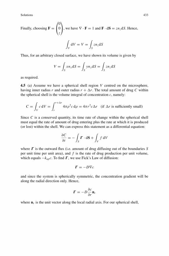
http://dx.doi.org/10.1007/978-3-642-54801-7_4

Solutions 433

Finally, choosing F =⎛⎝00z

⎞⎠, we have ∇ · F = 1 and F · dS = znzdS. Hence,

∫VdV = V =

∫SznzdS

Thus, for an arbitrary closed surface, we have shown its volume is given by

V =∫SxnxdS =

∫SynydS =

∫SznzdS

as required.

4.5 (a) Assume we have a spherical shell region V centred on the microsphere,having inner radius r and outer radius r + r . The total amount of drug C withinthe spherical shell is the volume integral of concentration c, namely:

C =∫Vc dV =

∫ r+ r

r4πρ2c dρ = 4πr2c r (if r is sufficiently small)

Since C is a conserved quantity, its time rate of change within the spherical shellmust equal the rate of amount of drug entering plus the rate at which it is produced(or lost) within the shell. We can express this statement as a differential equation:

∂C

∂t= −

∫SΓ · dS +

∫Vf dV

where Γ is the outward flux (i.e. amount of drug diffusing out of the boundaries Sper unit time per unit area), and f is the rate of drug production per unit volume,which equals −kupc. To find Γ , we use Fick’s Law of diffusion:

Γ = −D∇c

and since the system is spherically symmetric, the concentration gradient will bealong the radial direction only. Hence,

Γ = −D∂c

∂rnr

where nr is the unit vector along the local radial axis. For our spherical shell,

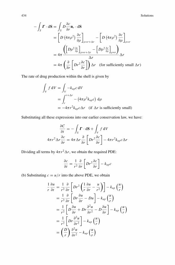
434 Solutions

−∫SΓ · dS =

∫SD

∂c

∂rnr · dS

=[D(4πρ2

) ∂c

∂ρ

]ρ=r+ r

−[D(4πρ2

) ∂c

∂ρ

]ρ=r

= 4π

([Dρ2 ∂c

∂ρ

]ρ=r+ r

−[Dρ2 ∂c

∂ρ

]ρ=r

)

r r

= 4π

(∂

∂r

[Dr2

∂c

∂r

]) r (for sufficiently small r)

The rate of drug production within the shell is given by

∫Vf dV =

∫V

−kupc dV

=∫ r+ r

r− (

4πρ2kupc)dρ

= −4πr2kupc r (if r is sufficiently small)

Substituting all these expressions into our earlier conservation law, we have:

∂C

∂t= −

∫SΓ · dS +

∫Vf dV

4πr2 r∂c

∂r= 4π r

∂

∂r

[Dr2

∂c

∂r

]− 4πr2kupc r

Dividing all terms by 4πr2 r , we obtain the required PDE:

∂c

∂t= 1

r2∂

∂r

[Dr2

∂c

∂r

]− kupc

(b) Substituting c = u/r into the above PDE, we obtain

1

r

∂u

∂t= 1

r2∂

∂r

[Dr2

(1

r

∂u

∂r− u

r2

)]− kup

(ur

)

= 1

r2∂

∂r

[Dr

∂u

∂r− Du

]− kup

(ur

)

= 1

r2

[D

∂u

∂r+ Dr

∂2u

∂r2− D

∂u

∂r

]− kup

(ur

)

= 1

r2

[Dr

∂2u

∂r2

]− kup

(ur

)

=(D

r

)∂2u

∂r2− kup

(ur

)

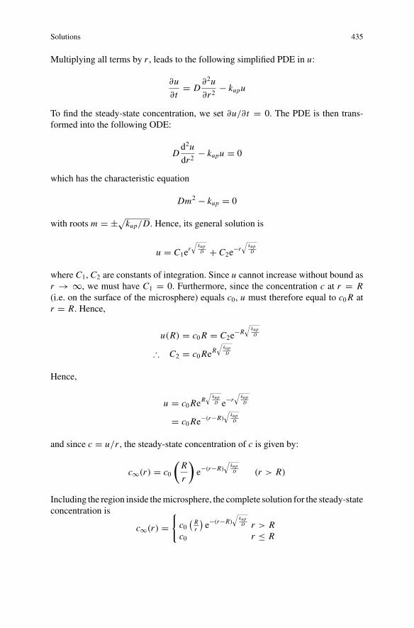
Solutions 435

Multiplying all terms by r , leads to the following simplified PDE in u:

∂u

∂t= D

∂2u

∂r2− kupu

To find the steady-state concentration, we set ∂u/∂t = 0. The PDE is then trans-formed into the following ODE:

Dd2u

dr2− kupu = 0

which has the characteristic equation

Dm2 − kup = 0

with roots m = ±√kup/D. Hence, its general solution is

u = C1er√

kupD + C2e

−r√

kupD

where C1, C2 are constants of integration. Since u cannot increase without bound asr → ∞, we must have C1 = 0. Furthermore, since the concentration c at r = R(i.e. on the surface of the microsphere) equals c0, u must therefore equal to c0R atr = R. Hence,

u(R) = c0R = C2e−R

√kupD

∴ C2 = c0ReR√

kupD

Hence,

u = c0ReR√

kupD e−r

√kupD

= c0Re−(r−R)

√kupD

and since c = u/r , the steady-state concentration of c is given by:

c∞(r) = c0

(R

r

)e−(r−R)

√kupD (r > R)

Including the region inside themicrosphere, the complete solution for the steady-stateconcentration is

c∞(r) ={c0(Rr

)e−(r−R)

√kupD r > R

c0 r ≤ R

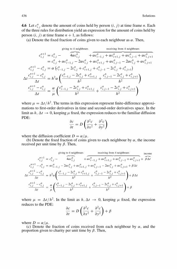
436 Solutions

4.6 Let cni, j denote the amount of coins held by person (i, j) at time frame n. Eachof the three rules for distribution yield an expression for the amount of coins held byperson (i, j) at time frame n + 1, as follows:

(a) Denote the fixed fraction of coins given to each neighbour as α. Then,

cn+1i, j = cni, j −

giving to 4 neighbours︷︸︸︷4αcni, j +

receiving from 4 neighbours︷︸︸︷αcni−1, j + αcni+1, j + αcni, j−1 + αcni, j+1

= cni, j + αcni−1, j − 2αcni, j + αcni+1, j + αcni, j−1 − 2αcni, j + αcni, j+1

cn+1i, j − cni, j = α

(cni−1, j − 2cni, j + cni+1, j + cni, j−1 − 2cni, j + cni, j+1

)

tcn+1i, j − cni, j

t= h2α

(cni−1, j − 2cni, j + cni+1, j

h2+ cni, j−1 − 2cni, j + cni, j+1

h2

)

cn+1i, j − cni, j

t= α

μ


h2+ cni, j−1 − 2cni, j + cni, j+1

h2

)

where μ = t/h2. The terms in this expression represent finite-difference approxi-mations to first-order derivatives in time and second-order derivatives space. In thelimit as h, t → 0, keeping μ fixed, the expression reduces to the familiar diffusionPDE:

∂c

∂t= D

(∂2c

∂x2+ ∂2c

∂y2

)

where the diffusion coefficient D = α/μ.(b) Denote the fixed fraction of coins given to each neighbour by α, the income

received per unit time by β. Then,



receiving from 4 neighbours︷︸︸︷αcni−1, j + αcni+1, j + αcni, j−1 + αcni, j+1 +

income︷︸︸︷β t

cn+1i, j − cni, j = αcni−1, j − 2αcni, j + αcni+1, j + αcni, j−1 − 2αcni, j + αcni, j+1 + β t


t= h2α


h2+

cni, j−1 − 2cni, j + cni, j+1

h2

)+ β t

cn+1i, j − cni, j

t= α

μ


h2+

cni, j−1 − 2cni, j + cni, j+1

h2

)+ β

where μ = t/h2. In the limit as h, t → 0, keeping μ fixed, the expressionreduces to the PDE:

∂c

∂t= D

(∂2c

∂x2+ ∂2c

∂y2

)+ β

where D = α/μ.(c) Denote the fraction of coins received from each neighbour by α, and the

proportion given to charity per unit time by β. Then,

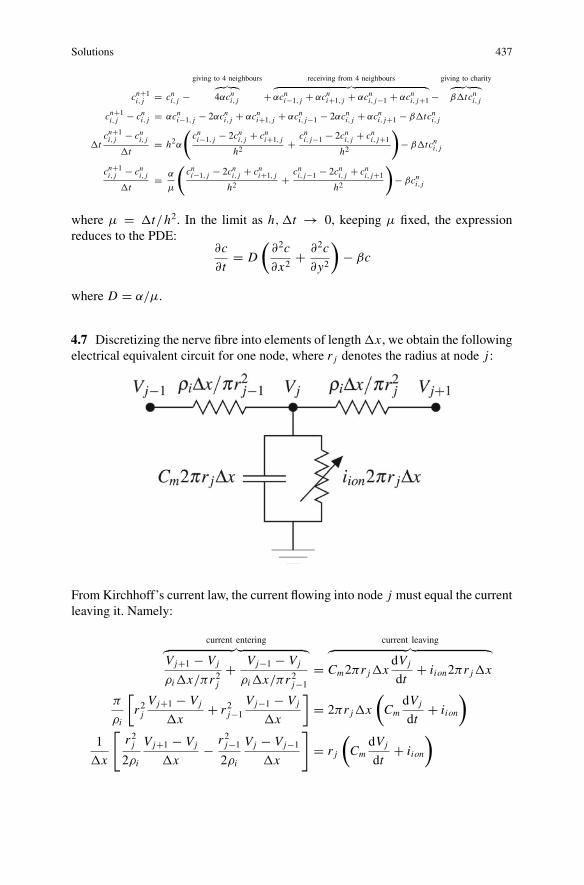
Solutions 437



receiving from 4 neighbours︷︸︸︷αcni−1, j + αcni+1, j + αcni, j−1 + αcni, j+1 −

giving to charity︷︸︸︷β tcni, j

cn+1i, j − cni, j = αcni−1, j − 2αcni, j + αcni+1, j + αcni, j−1 − 2αcni, j + αcni, j+1 − β tcni, j


t= h2α


h2+ cni, j−1 − 2cni, j + cni, j+1

h2

)− β tcni, j

cn+1i, j − cni, j

t= α

μ


h2+ cni, j−1 − 2cni, j + cni, j+1

h2

)− βcni, j

where μ = t/h2. In the limit as h, t → 0, keeping μ fixed, the expressionreduces to the PDE:

∂c

∂t= D

(∂2c

∂x2+ ∂2c

∂y2

)− βc

where D = α/μ.

4.7 Discretizing the nerve fibre into elements of length x , we obtain the followingelectrical equivalent circuit for one node, where r j denotes the radius at node j :

From Kirchhoff’s current law, the current flowing into node j must equal the currentleaving it. Namely:

current entering︷︸︸︷Vj+1 − Vj

ρi x/πr2j+ Vj−1 − Vj

ρi x/πr2j−1

=

current leaving︷︸︸︷Cm2πr j x

dVj

dt+ iion2πr j x

π

ρi

[r2j

Vj+1 − Vj

x+ r2j−1

Vj−1 − Vj

x

]= 2πr j x

(Cm

dVj

dt+ iion

)

1

x

[r2j2ρi

Vj+1 − Vj

x− r2j−1

2ρi

Vj − Vj−1

x

]= r j

(Cm

dVj

dt+ iion

)

438 Solutions

In the limit as x → 0, the above finite difference expressions approximate to thefollowing PDE:

∂

∂x

[r2

2ρi

∂V

∂x

]= r

(Cm

∂V

∂t+ iion

)

or to be compatible with COMSOL’s general PDE form:

rCm∂V

∂t+ ∂

∂x

[− r2

2ρi

∂V

∂x

]= −riion

4.8 To derive the underlying PDE for the muscle displacement, we discretize themuscle strand into N sub-units, each of length x = L/N . We can therefore char-acterise N + 1 nodes, each having displacement ui (i = 0 · · · N ). Denoting thechange in length of the i th sub-unit by li , and its corresponding l1, l2 values by l1i ,l2i respectively. Then the following relationships hold:

li = l1i + l2i = ui − ui−1

Fi = ( k1 x

)l1i for the series element

Fi = ( k2 x

)l2i + (

b x

) dl2idt for the parallel spring/dashpot

where Fi is the passive force generated by the i th sub-unit, which acts on the pointmasses to oppose the changes in length. Fi is the same for both the series spring andthe parallel spring/dashpot combination in the i th sub-unit, since these elements arein series. Re-arranging the last two of the above relationships, we obtain:

l1i =(Fik1

) x

l2i =(Fik2

) x −

(b

k2

)dl2idt

Adding these together yields:

l1i + l2i =(1

k1+ 1

k2

)Fi x −

(b

k2

)dl2idt

li =(1

k1+ 1

k2

)Fi x −

(b

k2

)dl2idt

=(1

k1+ 1

k2

)Fi x −

(b

k2

)[dlidt

− dl1idt

]

and using the series element relationship Fi = (k1/ x)l1i , we obtain dFi/dt =(k1/ x)dl1i/dt and hence dl1i/dt = ( x/k1)dFi/dt . Substituting the latter into theabove expression, we obtain:

Solutions 439

li =(1

k1+ 1

k2

)Fi x −

(b

k2

)[dlidt

− x

k1

dF

dt

]

li +(b

k2

)dlidt

=(1

k1+ 1

k2

)Fi x +

(b

k1k2

)dF

dt x

Multiplying throughout by k1k1/ x and re-arranging terms, yields:

(1

x

)[bk1

dlidt

+ k1k2li

]= b

dFidt

+ (k1 + k2)Fi

Finally, substituting li = ui − ui−1, we obtain:

(1

x

)[bk1

(duidt

− dui−1

dt

)+ k1k2(ui − ui−1)

]= b

dFidt

+ (k1 + k2)Fi (B.1)

A similar relation holds also for the (i + 1)th sub-unit:

(1

x

)[bk1

(dui+1

dt− dui

dt

)+ k1k2(ui+1 − ui )

]= b

dFi+1

dt+ (k1 + k2)Fi+1

(B.2)The total force acting on point mass i is given by

Fi+1 − Fi = (M x)d2uidt2

Therefore, subtracting Eq.B.1 from Eq.B.2, we obtain:

(1

x

)[bk1

(dui+1

dt− dui

dt+ dui−1

dt

)+ k1k2(ui+1 − 2ui + ui−1)

]

= b

(dFi+1

dt− dFi

dt

)+ (k1 + k2)

[Fi+1 − Fi

]

= bM xd

dt

[d2uidt2

]+ (k1 + k2)M x

d2uidt2

Dividing both sides by x :

bk1d

dt

[ui+1 − 2ui + ui−1

2x

]+ k1k2

(ui+1 − 2ui + ui−1

2x

)

= bMd

dt

[d2uidt2

]+ (k1 + k2)M

d2uidt2

In the limit as x → 0, this expression reduces to the PDE:

bk1∂

∂t

[∂2u

∂x2

]+ k1k2

∂2u

∂x2= bM

∂3u

∂t3+ (k1 + k2)M

∂2u

∂t2

440 Solutions

where x is the spatial coordinate along the length of the muscle. Re-arranging terms,the above PDE can also be re-written as:

b∂

∂t

[k1

∂2u

∂x2− M

∂2u

∂t2

]+ k2

(k1

∂2u

∂x2− M

∂2u

∂t2

)= k1M

∂2u

∂t2

4.9 (a) To solve the atrial tissue PDE system using the method of lines, we firstdiscretize the 2D domain into a square grid of size N × N . There will therefore bea total of N 2 individual nodes, with 2N 2 variables to be solved for (i.e. Vm and u ateach node). The following PDE must be discretized:

βCm

(∂Vm

∂t

)= ∇ · (σ∇Vm) − βiion + istim

= σ

(∂2Vm

∂x2+ ∂2Vm

∂y2

)− βiion + istim (since σ is constant)

∴ ∂Vm

∂t= σ

βCm

(∂2Vm

∂x2+ ∂2Vm

∂y2

)− iion

Cm+ istim

βCm

Denoting Vm and u for the (i, j)th node as Vi, j and ui, j respectively, this PDE canbe discretized as:

dVi, jdt

= σ

βCm

[Vi, j+1 − 2Vi, j + Vi, j−1

h2+ Vi+1, j − 2Vi, j + Vi−1, j

h2

]− iion,i, j

Cm+ istim,i, j

βCm

= σ

βCm

[Vi, j+1 + Vi, j−1 + Vi+1, j + Vi−1, j − 4Vi, j

h2

]− iion,i, j

Cm+ istim,i, j

βCm

where iion,i, j and istim,i, j are ii on and is t im evaluated at node (i, j). To setup thissystem in Matlab, its in-built ode solvers require the independent variables to bein a single-column array format. Denoting this array by Y, we can assign the firstN 2 elements to the Vm variables and the final N 2 elements for the u, according thefollowing “map”:

Vi, j = Y(i−1)N+ j

ui, j = YN 2+(i−1)N+ j

with i, j = 1 · · · N . To implement the zero-flux boundary conditions on the externalboundaries, we set the Vm value of points exterior to the boundary to its value at theadjacent boundary point. InMatlab, this can be achieved by padding the 2D Vm-arraywith extra rows and columns whose Vm values are equal to the adjacent boundary.

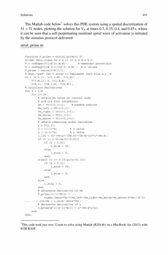
Solutions 441

The Matlab code below7 solves this PDE system using a spatial discretization of51× 51 nodes, plotting the solution for Vm at times 0.3, 0.35, 0.4, and 0.45 s, whereit can be seen that a self-perpetuating reentrant spiral wave of activation is initiatedby the stimulus protocol delivered.

atrial_prime.m:

function Y_prime = atrial_prime(t,Y)global beta sigma Cm a b c1 c2 A B d e N hV = reshape(Y(1:Nˆ2),N,N)’; % membrane potentialsU = reshape(Y(Nˆ2+1:2*Nˆ2),N,N)’; % u valuesY_prime = zeros(2*Nˆ2,1);% Next,"pad" the V array to implement zero-flux b.c.’sVV = [V(1,1), V(1,1:N), V(1,N); ...

V(1:N,1), V, V(1:N,N); ...V(N,1), V(N,1:N), V(N,N)];

% calculate derivativesfor i = 1:N

for j=1:N% obtain Vm value of current node% and its four neighboursVm = VV(i+1,j+1); % padded indicesVm_left = VV(i+1,j);Vm_right = VV(i+1,j+2);Vm_below = VV(i,j+1);Vm_above = VV(i+2,j+1);% obtain remaining nodal variablesu = U(i,j);x = (j-1)*h; % x valuey = (i-1)*h; % y valuei_ion = c1*(Vm-a)*(Vm-A)*(Vm-B)+c2*u*(Vm-B);if (t >= 0.01)&&(t<=0.011)

if (y < 0.01)i_stim = 50;

elsei_stim = 0;

end;elseif (t >= 0.15)&&(t<=0.151)

if (x < 0.01)i_stim = 50;

elsei_stim = 0;

end;else

i_stim = 0;end;% determine derivative of VmY_prime((i-1)*N+j) = ...

sigma/(beta*Cm)*(Vm_left+Vm_right+Vm_below+Vm_above-4*Vm)/(hˆ2)... - i_ion/Cm + i_stim/(beta*Cm);

% determine derivative of uY_prime(Nˆ2+(i-1)*N+j) = e*(Vm-d*u-b);

end;end;

7This code took just over 12min to solve using Matlab (R2014b) on a MacBook Air (2013) with8GB RAM.

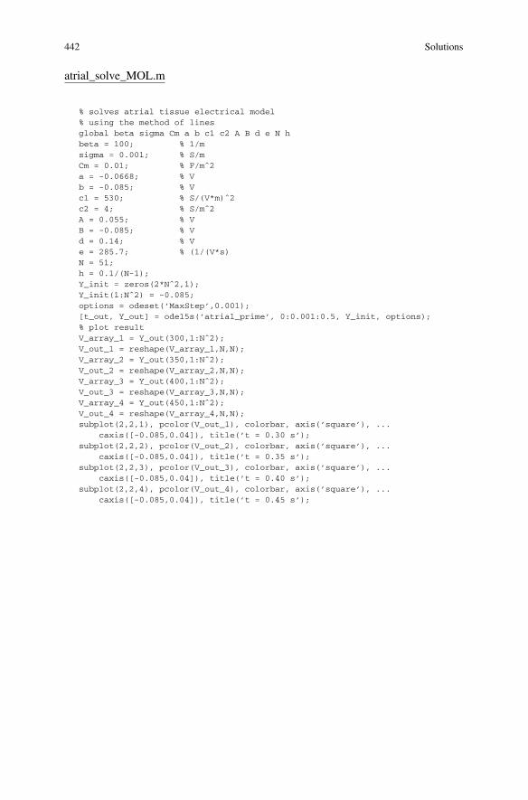
442 Solutions

atrial_solve_MOL.m

% solves atrial tissue electrical model% using the method of linesglobal beta sigma Cm a b c1 c2 A B d e N hbeta = 100; % 1/msigma = 0.001; % S/mCm = 0.01; % F/mˆ2a = -0.0668; % Vb = -0.085; % Vc1 = 530; % S/(V*m)ˆ2c2 = 4; % S/mˆ2A = 0.055; % VB = -0.085; % Vd = 0.14; % Ve = 285.7; % (1/(V*s)N = 51;h = 0.1/(N-1);Y_init = zeros(2*Nˆ2,1);Y_init(1:Nˆ2) = -0.085;options = odeset(’MaxStep’,0.001);[t_out, Y_out] = ode15s(’atrial_prime’, 0:0.001:0.5, Y_init, options);% plot resultV_array_1 = Y_out(300,1:Nˆ2);V_out_1 = reshape(V_array_1,N,N);V_array_2 = Y_out(350,1:Nˆ2);V_out_2 = reshape(V_array_2,N,N);V_array_3 = Y_out(400,1:Nˆ2);V_out_3 = reshape(V_array_3,N,N);V_array_4 = Y_out(450,1:Nˆ2);V_out_4 = reshape(V_array_4,N,N);subplot(2,2,1), pcolor(V_out_1), colorbar, axis(’square’), ...

caxis([-0.085,0.04]), title(’t = 0.30 s’);subplot(2,2,2), pcolor(V_out_2), colorbar, axis(’square’), ...



caxis([-0.085,0.04]), title(’t = 0.45 s’);

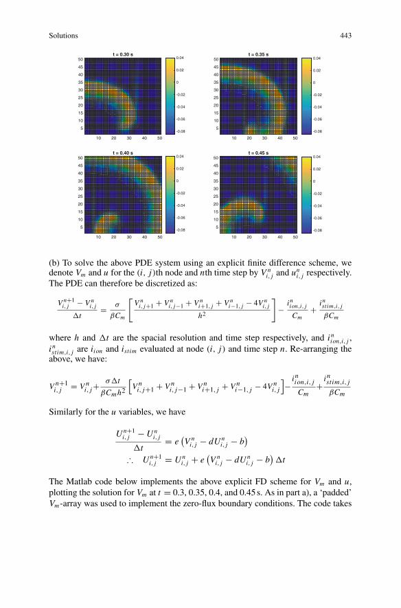
Solutions 443

10 20 30 40 50

5

10

15

20

25

30

35

40

45

50t = 0.30 s

-0.08

-0.06

-0.04

-0.02

0

0.02

0.04

10 20 30 40 50

5

10

15

20

25

30

35

40

45

50t = 0.35 s

-0.08

-0.06

-0.04

-0.02

0

0.02

0.04

10 20 30 40 50

5

10

15

20

25

30

35

40

45

50t = 0.40 s

-0.08

-0.06

-0.04

-0.02

0

0.02

0.04

10 20 30 40 50

5

10

15

20

25

30

35

40

45

50t = 0.45 s

-0.08

-0.06

-0.04

-0.02

0

0.02

0.04

(b) To solve the above PDE system using an explicit finite difference scheme, wedenote Vm and u for the (i, j)th node and nth time step by V n

i, j and uni, j respectively.

The PDE can therefore be discretized as:

V n+1i, j − V n

i, j

t= σ

βCm

[V ni, j+1 + V n

i, j−1 + V ni+1, j + V n

i−1, j − 4V ni, j

h2

]− inion,i, j

Cm+ instim,i, j

βCm

where h and t are the spacial resolution and time step respectively, and i nion,i, j ,i nstim,i, j are iion and istim evaluated at node (i, j) and time step n. Re-arranging theabove, we have:

Vn+1i, j = Vn

i, j+σ t

βCmh2

[Vni, j+1 + Vn

i, j−1 + Vni+1, j + Vn

i−1, j − 4Vni, j

]−inion,i, j

Cm+instim,i, j

βCm

Similarly for the u variables, we have

Un+1i, j −Un

i, j

t= e

(V ni, j − dUn

i, j − b)

∴ Un+1i, j = Un

i, j + e(V ni, j − dUn

i, j − b) t

The Matlab code below implements the above explicit FD scheme for Vm and u,plotting the solution for Vm at t = 0.3, 0.35, 0.4, and 0.45 s. As in part a), a ‘padded’Vm-array was used to implement the zero-flux boundary conditions. The code takes

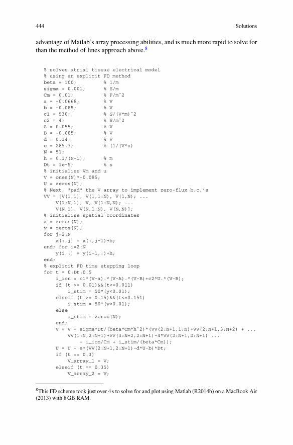
444 Solutions

advantage of Matlab’s array processing abilities, and is much more rapid to solve forthan the method of lines approach above.8

% solves atrial tissue electrical model% using an explicit FD methodbeta = 100; % 1/msigma = 0.001; % S/mCm = 0.01; % F/mˆ2a = -0.0668; % Vb = -0.085; % Vc1 = 530; % S/(V*m)ˆ2c2 = 4; % S/mˆ2A = 0.055; % VB = -0.085; % Vd = 0.14; % Ve = 285.7; % (1/(V*s)N = 51;h = 0.1/(N-1); % mDt = 1e-5; % s% initialise Vm and uV = ones(N)*-0.085;U = zeros(N);% Next, "pad" the V array to implement zero-flux b.c.’sVV = [V(1,1), V(1,1:N), V(1,N); ...

V(1:N,1), V, V(1:N,N); ...V(N,1), V(N,1:N), V(N,N)];

% initialise spatial coordinatesx = zeros(N);y = zeros(N);for j=2:N

x(:,j) = x(:,j-1)+h;end; for i=2:N

y(i,:) = y(i-1,:)+h;end;% explicit FD time stepping loopfor t = 0:Dt:0.5

i_ion = c1*(V-a).*(V-A).*(V-B)+c2*U.*(V-B);if (t >= 0.01)&&(t<=0.011)

i_stim = 50*(y<0.01);elseif (t >= 0.15)&&(t<=0.151)

i_stim = 50*(y<0.01);else

i_stim = zeros(N);end;V = V + sigma*Dt/(beta*Cm*hˆ2)*(VV(2:N+1,1:N)+VV(2:N+1,3:N+2) + ...

VV(1:N,2:N+1)+VV(3:N+2,2:N+1)-4*VV(2:N+1,2:N+1) ...- i_ion/Cm + i_stim/(beta*Cm));

U = U + e*(VV(2:N+1,2:N+1)-d*U-b)*Dt;if (t == 0.3)

V_array_1 = V;elseif (t == 0.35)

V_array_2 = V;

8This FD scheme took just over 4 s to solve for and plot using Matlab (R2014b) on a MacBook Air(2013) with 8GB RAM.

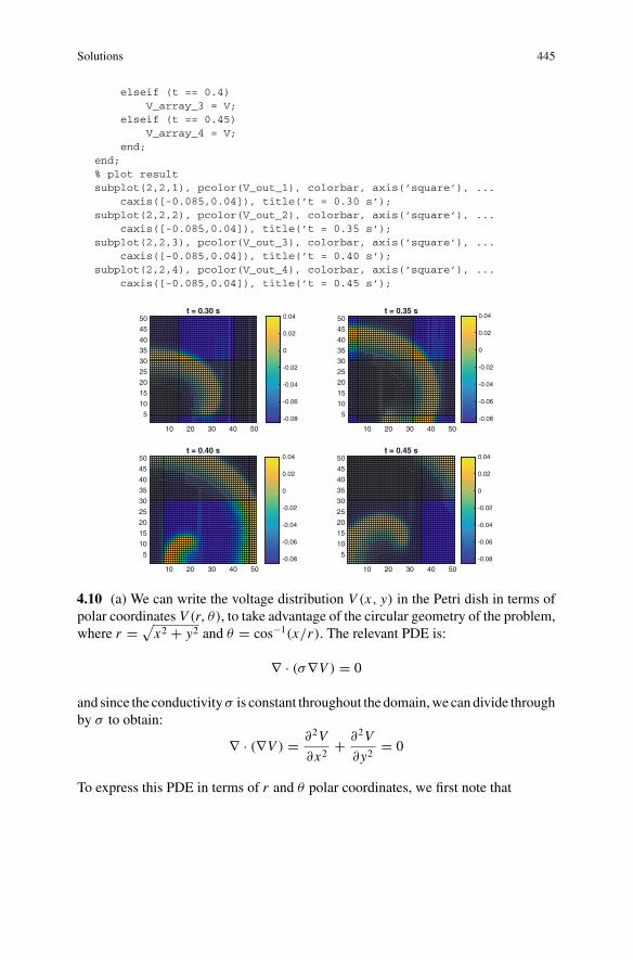
Solutions 445

elseif (t == 0.4)V_array_3 = V;

elseif (t == 0.45)V_array_4 = V;

end;end;% plot resultsubplot(2,2,1), pcolor(V_out_1), colorbar, axis(’square’), ...




caxis([-0.085,0.04]), title(’t = 0.45 s’);

10 20 30 40 50

5

10

15

20

25

30

35

40

45

50t = 0.30 s

-0.08

-0.06

-0.04

-0.02

0

0.02

0.04

10 20 30 40 50

5

10

15

20

25

30

35

40

45

50t = 0.35 s

-0.08

-0.06

-0.04

-0.02

0

0.02

0.04

10 20 30 40 50

5

10

15

20

25

30

35

40

45

50t = 0.40 s

-0.08

-0.06

-0.04

-0.02

0

0.02

0.04

10 20 30 40 50

5

10

15

20

25

30

35

40

45

50t = 0.45 s

-0.08

-0.06

-0.04

-0.02

0

0.02

0.04

4.10 (a) We can write the voltage distribution V (x, y) in the Petri dish in terms ofpolar coordinates V (r, θ), to take advantage of the circular geometry of the problem,where r = √

x2 + y2 and θ = cos−1(x/r). The relevant PDE is:

∇ · (σ∇V ) = 0

and since the conductivityσ is constant throughout the domain,we can divide throughby σ to obtain:

∇ · (∇V ) = ∂2V

∂x2+ ∂2V

∂y2= 0

To express this PDE in terms of r and θ polar coordinates, we first note that

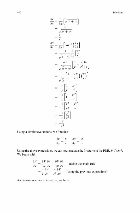
446 Solutions

∂r

∂x= ∂

∂x

[√x2 + y2

]

= x√x2 + y2

= x

r∂θ

∂x= ∂

∂x

[cos−1

( xr

)]

= −1√1 − x2

r2

∂

∂x

[ xr

]

= −1√r2r2 − x2

r2

[1

r− x

r2∂r

∂x

]

= −1√y2

r2

[1

r−( x

r2

) ( xr

)]

= − r

y

[1

r− x2

r3

]

= −1

y

[1 − x2

r2

]

= −1

y

[r2

r2− x2

r2

]

= −1

y

[y2

r2

]

= − y

r2

Using a similar evaluations, we find that

∂r

∂y= y

r

∂θ

∂y= x

r2

Using the above expressions,we can nowevaluate the first termof the PDE, ∂2V/∂x2.We begin with:

∂V

∂x= ∂V

∂r

∂r

∂x+ ∂V

∂θ

∂θ

∂x(using the chain rule)

= x

r

∂V

∂r− y

r2∂V

∂θ(using the previous expressions)

And taking one more derivative, we have:

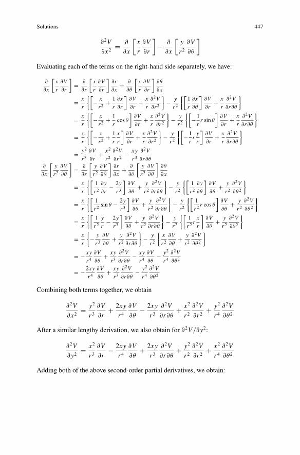
Solutions 447

∂2V

∂x2= ∂

∂x

[x

r

∂V

∂r

]− ∂

∂x

[y

r2∂V

∂θ

]

Evaluating each of the terms on the right-hand side separately, we have:

∂

∂x

[x

r

∂V

∂r

]= ∂

∂r

[x

r

∂V

∂r

]∂r

∂x+ ∂

∂θ

[x

r

∂V

∂r

]∂θ

∂x

= x

r

{[− x

r2+ 1

r

∂x

∂r

]∂V

∂r+ x

r

∂2V

∂r2

}− y

r2

{[1

r

∂x

∂θ

]∂V

∂r+ x

r

∂2V

∂r∂θ

}

= x

r

{[− x

r2+ 1

rcos θ

]∂V

∂r+ x

r

∂2V

∂r2

}− y

r2

{[−1

rr sin θ

]∂V

∂r+ x

r

∂2V

∂r∂θ

}

= x

r

{[− x

r2+ 1

r

x

r

]∂V

∂r+ x

r

∂2V

∂r2

}− y

r2

{[−1

rry

r

]∂V

∂r+ x

r

∂2V

∂r∂θ

}

= y2

r3∂V

∂r+ x2

r2∂2V

∂r2− xy

r3∂2V

∂r∂θ

∂

∂x

[y

r2∂V

∂θ

]= ∂

∂r

[y

r2∂V

∂θ

]∂r

∂x+ ∂

∂θ

[y

r2∂V

∂θ

]∂θ

∂x

= x

r

{[1

r2∂y

∂r− 2y

r3

]∂V

∂θ+ y

r2∂2V

∂r∂θ

}− y

r2

{[1

r2∂y

∂θ

]∂V

∂θ+ y

r2∂2V

∂θ2

}

= x

r

{[1

r2sin θ − 2y

r3

]∂V

∂θ+ y

r2∂2V

∂r∂θ

}− y

r2

{[1

r2r cos θ

]∂V

∂θ+ y

r2∂2V

∂θ2

}

= x

r

{[1

r2y

r− 2y

r3

]∂V

∂θ+ y

r2∂2V

∂r∂θ

}− y

r2

{[1

r2rx

r

]∂V

∂θ+ y

r2∂2V

∂θ2

}

= x

r

{− y

r3∂V

∂θ+ y

r2∂2V

∂r∂θ

}− y

r2

{x

r2∂V

∂θ+ y

r2∂2V

∂θ2

}

= − xy

r4∂V

∂θ+ xy

r3∂2V

∂r∂θ− xy

r4∂V

∂θ− y2

r4∂2V

∂θ2

= −2xy

r4∂V

∂θ+ xy

r3∂2V

∂r∂θ− y2

r4∂2V

∂θ2

Combining both terms together, we obtain

∂2V

∂x2= y2

r3∂V

∂r+ 2xy

r4∂V

∂θ− 2xy

r3∂2V

∂r∂θ+ x2

r2∂2V

∂r2+ y2

r4∂2V

∂θ2

After a similar lengthy derivation, we also obtain for ∂2V/∂y2:

∂2V

∂y2= x2

r3∂V

∂r− 2xy

r4∂V

∂θ+ 2xy

r3∂2V

∂r∂θ+ y2

r2∂2V

∂r2+ x2

r4∂2V

∂θ2

Adding both of the above second-order partial derivatives, we obtain:

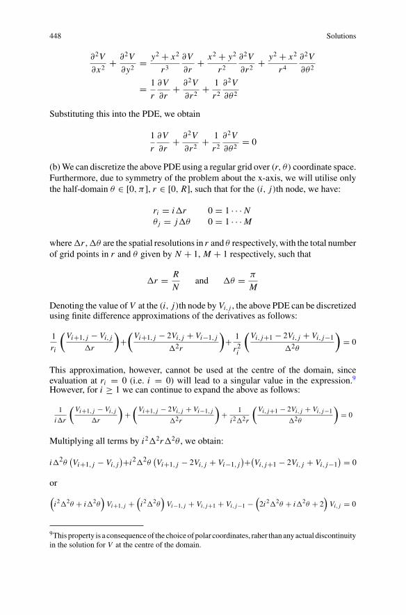
448 Solutions

∂2V

∂x2+ ∂2V

∂y2= y2 + x2

r3∂V

∂r+ x2 + y2

r2∂2V

∂r2+ y2 + x2

r4∂2V

∂θ2

= 1

r

∂V

∂r+ ∂2V

∂r2+ 1

r2∂2V

∂θ2

Substituting this into the PDE, we obtain

1

r

∂V

∂r+ ∂2V

∂r2+ 1

r2∂2V

∂θ2= 0

(b)We can discretize the above PDE using a regular grid over (r, θ) coordinate space.Furthermore, due to symmetry of the problem about the x-axis, we will utilise onlythe half-domain θ ∈ [0, π ], r ∈ [0, R], such that for the (i, j)th node, we have:

ri = i r 0 = 1 · · · Nθ j = j θ 0 = 1 · · · M

where r , θ are the spatial resolutions in r and θ respectively, with the total numberof grid points in r and θ given by N + 1, M + 1 respectively, such that

r = R

Nand θ = π

M

Denoting the value of V at the (i, j)th node by Vi, j , the above PDE can be discretizedusing finite difference approximations of the derivatives as follows:

1

ri

(Vi+1, j − Vi, j

r

)+(Vi+1, j − 2Vi, j + Vi−1, j

2r

)+ 1

r2i

(Vi, j+1 − 2Vi, j + Vi, j−1

2θ

)= 0

This approximation, however, cannot be used at the centre of the domain, sinceevaluation at ri = 0 (i.e. i = 0) will lead to a singular value in the expression.9However, for i ≥ 1 we can continue to expand the above as follows:

1

i r

(Vi+1, j − Vi, j

r

)+(Vi+1, j − 2Vi, j + Vi−1, j

2r

)+ 1

i2 2r

(Vi, j+1 − 2Vi, j + Vi, j−1

2θ

)= 0

Multiplying all terms by i2 2r 2θ , we obtain:

i 2θ(Vi+1, j − Vi, j

)+i2 2θ(Vi+1, j − 2Vi, j + Vi−1, j

)+(Vi, j+1 − 2Vi, j + Vi, j−1

) = 0

or(i2 2θ + i 2θ

)Vi+1, j +

(i2 2θ

)Vi−1, j + Vi, j+1 + Vi, j−1 −

(2i2 2θ + i 2θ + 2

)Vi, j = 0

9This property is a consequenceof the choice of polar coordinates, raher than anyactual discontinuityin the solution for V at the centre of the domain.

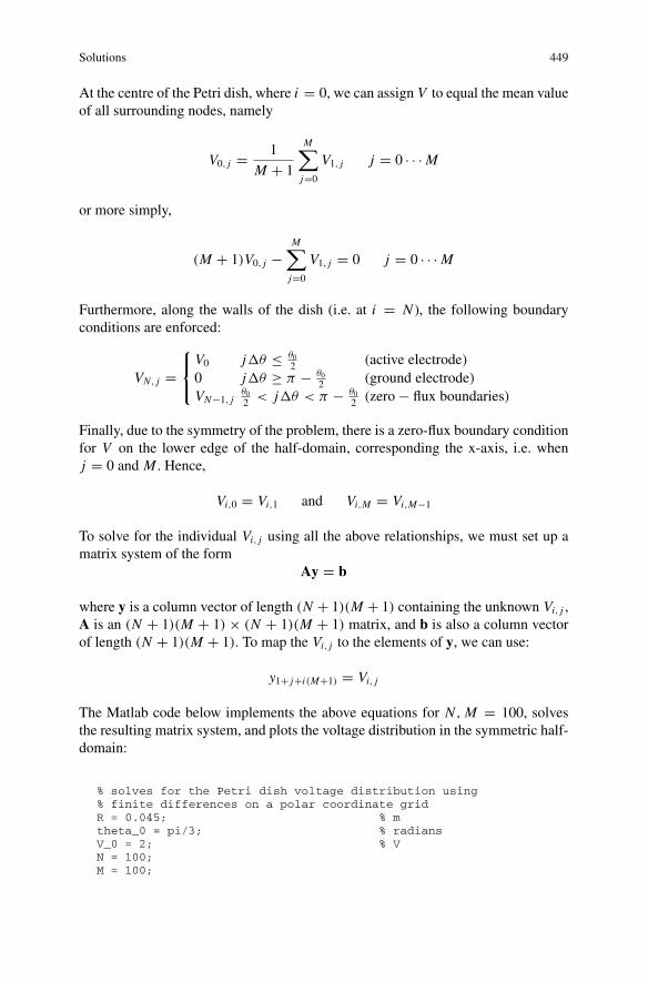
Solutions 449

At the centre of the Petri dish, where i = 0, we can assign V to equal the mean valueof all surrounding nodes, namely

V0, j = 1

M + 1

M∑j=0

V1, j j = 0 · · · M

or more simply,

(M + 1)V0, j −M∑j=0

V1, j = 0 j = 0 · · · M

Furthermore, along the walls of the dish (i.e. at i = N ), the following boundaryconditions are enforced:

VN , j =⎧⎨⎩V0 j θ ≤ θ0

2 (active electrode)0 j θ ≥ π − θ0

2 (ground electrode)VN−1, j

θ02 < j θ < π − θ0

2 (zero − flux boundaries)

Finally, due to the symmetry of the problem, there is a zero-flux boundary conditionfor V on the lower edge of the half-domain, corresponding the x-axis, i.e. whenj = 0 and M . Hence,

Vi,0 = Vi,1 and Vi,M = Vi,M−1

To solve for the individual Vi, j using all the above relationships, we must set up amatrix system of the form

Ay = b

where y is a column vector of length (N + 1)(M + 1) containing the unknown Vi, j ,A is an (N + 1)(M + 1) × (N + 1)(M + 1) matrix, and b is also a column vectorof length (N + 1)(M + 1). To map the Vi, j to the elements of y, we can use:

y1+ j+i(M+1) = Vi, j

The Matlab code below implements the above equations for N , M = 100, solvesthe resulting matrix system, and plots the voltage distribution in the symmetric half-domain:

% solves for the Petri dish voltage distribution using% finite differences on a polar coordinate gridR = 0.045; % mtheta_0 = pi/3; % radiansV_0 = 2; % VN = 100;M = 100;

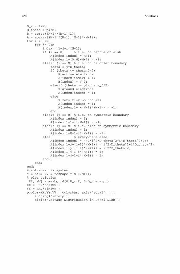
450 Solutions

D_r = R/N;D_theta = pi/M;B = zeros((N+1)*(M+1),1);A = sparse((N+1)*(M+1),(N+1)*(M+1));for i = 0:N

for j= 0:Mindex = 1+j+i*(M+1);if (i == 0) % i.e. at centre of dish

A(index,index) = M+1;A(index,1+(0:M)+M+1) = -1;

elseif (i == N) % i.e. on circular boundarytheta = j*D_theta;if (theta <= theta_0/2)

% active electrodeA(index,index) = 1;B(index) = V_0;

elseif (theta >= pi-theta_0/2)% ground electrodeA(index,index) = 1;

else% zero-flux boundariesA(index,index) = 1;A(index,1+j+(N-1)*(M+1)) = -1;

end;elseif (j == 0) % i.e. on symmetric boundary

A(index,index) = 1;A(index,1+1+i*(M+1)) = -1;

elseif (j == M) % i.e. also on symmetric boundaryA(index,index) = 1;A(index,1+M-1+i*(M+1)) = -1;

else % everywhere elseA(index,index) = -(2*iˆ2*D_thetaˆ2+i*D_thetaˆ2+2);A(index,1+j+(i+1)*(M+1)) = iˆ2*D_thetaˆ2+i*D_thetaˆ2;A(index,1+j+(i-1)*(M+1)) = iˆ2*D_thetaˆ2;A(index,1+j+1+i*(M+1)) = 1;A(index,1+j-1+i*(M+1)) = 1;

end;end;

end;% solve matrix systemY = A\B; VV = reshape(Y,N+1,M+1);% plot solution[RR, WW] = meshgrid(0:D_r:R, 0:D_theta:pi);XX = RR.*cos(WW);YY = RR.*sin(WW);pcolor(XX,YY,VV), colorbar, axis(’equal’),...

shading(’interp’),title(’Voltage Distribution in Petri Dish’);

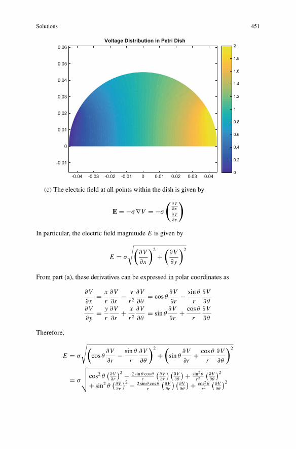
Solutions 451

-0.04 -0.03 -0.02 -0.01 0 0.01 0.02 0.03 0.04

-0.01

0

0.01

0.02

0.03

0.04

0.05

0.06Voltage Distribution in Petri Dish

0

0.2

0.4

0.6

0.8

1

1.2

1.4

1.6

1.8

2

(c) The electric field at all points within the dish is given by

E = −σ∇V = −σ

(∂V∂x∂V∂y

)

In particular, the electric field magnitude E is given by

E = σ

√(∂V

∂x

)2

+(

∂V

∂y

)2

From part (a), these derivatives can be expressed in polar coordinates as

∂V

∂x= x

r

∂V

∂r− y

r2∂V

∂θ= cos θ

∂V

∂r− sin θ

r

∂V

∂θ∂V

∂y= y

r

∂V

∂r+ x

r2∂V

∂θ= sin θ

∂V

∂r+ cos θ

r

∂V

∂θ

Therefore,

E = σ

√(cos θ

∂V

∂r− sin θ

r

∂V

∂θ

)2

+(sin θ

∂V

∂r+ cos θ

r

∂V

∂θ

)2

= σ

√√√√ cos2 θ(

∂V∂r

)2 − 2 sin θ cos θr

(∂V∂r

) (∂V∂θ

) + sin2 θr2

(∂V∂θ

)2+ sin2 θ

(∂V∂r

)2 − 2 sin θ cos θr

(∂V∂r

) (∂V∂θ

) + cos2 θr2

(∂V∂θ

)2

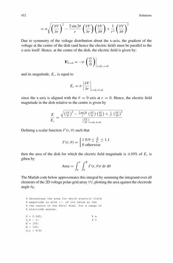
452 Solutions

= σ

√(∂V

∂r

)2

− 2 sin 2θ

r

(∂V

∂r

)(∂V

∂θ

)+ 1

r2

(∂V

∂θ

)2

Due to symmetry of the voltage distribution about the x-axis, the gradient of thevoltage at the centre of the dish (and hence the electric field) must be parallel to thex-axis itself. Hence, at the centre of the dish, the electric field is given by:

E|r=0 = −σ

(∂V∂x0

)∣∣∣∣x=0, y=0

and its magnitude, Ec, is equal to

Ec = σ

∣∣∣∣∂V∂r∣∣∣∣r=0, θ=0

since the x-axis is aligned with the θ = 0 axis at r = 0. Hence, the electric fieldmagnitude in the dish relative to the centre is given by

E

Ec=

√(∂V∂r

)2 − 2 sin 2θr

(∂V∂r

) (∂V∂θ

) + 1r2(

∂V∂θ

)2∣∣ ∂V

∂r

∣∣r=0, θ=0

Defining a scalar function Γ (r, θ) such that

Γ (r, θ) ={1 0.9 ≤ E

Ec≤ 1.1

0 otherwise

then the area of the dish for which the electric field magnitude is ±10% of Ec isgiben by

Area =∫ π

0

∫ R

0Γ (r, θ)r dr dθ

TheMatlab code below approximates this integral by summing the integrand over allelements of the 2D voltage polar-grid array VV, plotting the area against the electrodeangle θ0:

% Determines the area for which electric field% magnitude is with +/- of its value at the% the centre of the Petri dish, for a range of% electrode angles.

R = 0.045; % mV_0 = 2; % VN = 100;M = 100;D_r = R/N;

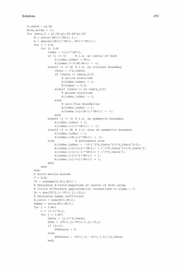
Solutions 453

D_theta = pi/M;Area_array = [];for theta_0 = pi/50:pi/50:49*pi/50

B = zeros((N+1)*(M+1),1);A = sparse((N+1)*(M+1),(N+1)*(M+1));for i = 0:N

for j= 0:Mindex = 1+j+i*(M+1);if (i == 0) % i.e. at centre of dish

A(index,index) = M+1;A(index,1+(0:M)+M+1) = -1;

elseif (i == N) % i.e. on circular boundarytheta = j*D_theta;if (theta <= theta_0/2)

% active electrodeA(index,index) = 1;B(index) = V_0;

elseif (theta >= pi-theta_0/2)% ground electrodeA(index,index) = 1;

else% zero-flux boundariesA(index,index) = 1;A(index,1+j+(N-1)*(M+1)) = -1;

end;elseif (j == 0) % i.e. on symmetric boundary

A(index,index) = 1;A(index,1+1+i*(M+1)) = -1;

elseif (j == M) % i.e. also on symmetric boundaryA(index,index) = 1;A(index,1+M-1+i*(M+1)) = -1;

else % everywhere elseA(index,index) = -(2*iˆ2*D_thetaˆ2+i*D_thetaˆ2+2);A(index,1+j+(i+1)*(M+1)) = iˆ2*D_thetaˆ2+i*D_thetaˆ2;A(index,1+j+(i-1)*(M+1)) = iˆ2*D_thetaˆ2;A(index,1+j+1+i*(M+1)) = 1;A(index,1+j-1+i*(M+1)) = 1;

end;end;

end;% solve matrix systemY = A\B;VV = reshape(Y,N+1,M+1)’;% Determine E-field magnitude at centre of disk using% finite difference approximation (normalised to sigma = 1)Ec = abs(VV(2,1)-VV(1,1))/D_r;% Determine Gamma coefficientE_ratio = ones(N+1,M+1);Gamma = zeros(N+1,M+1);for i = 2:N+1

r = (i-1)*D_r;for j = 1:M+1

theta = (j-1)*D_theta;dVdr = (VV(i,j)-VV(i-1,j))/D_r;if (j==1)

dVdtheta = 0;else

dVdtheta = (VV(i,j)- VV(i,j-1))/D_theta;end;

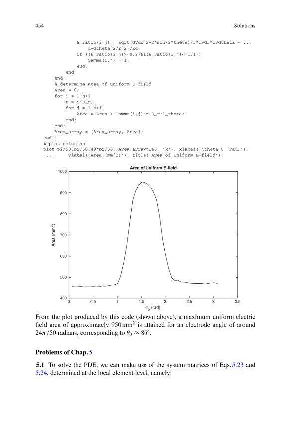
454 Solutions

E_ratio(i,j) = sqrt(dVdrˆ2-2*sin(2*theta)/r*dVdr*dVdtheta + ...dVdthetaˆ2/rˆ2)/Ec;

if ((E_ratio(i,j)>=0.9)&&(E_ratio(i,j)<=1.1))Gamma(i,j) = 1;

end;end;

end;% determine area of uniform E-fieldArea = 0;for i = 1:N+1

r = i*D_r;for j = 1:M+1

Area = Area + Gamma(i,j)*r*D_r*D_theta;end;

end;Area_array = [Area_array, Area];

end;% plot solutionplot(pi/50:pi/50:49*pi/50, Area_array*1e6, ’k’), xlabel(’\theta_0 (rad)’),... ylabel(’Area (mmˆ2)’), title(’Area of Uniform E-field’);

From the plot produced by this code (shown above), a maximum uniform electricfield area of approximately 950mm2 is attained for an electrode angle of around24π/50 radians, corresponding to θ0 ≈ 86◦.

Problems of Chap.5

5.1 To solve the PDE, we can make use of the system matrices of Eqs. 5.23 and5.24, determined at the local element level, namely:

http://dx.doi.org/10.1007/978-3-642-54801-7_5

http://dx.doi.org/10.1007/978-3-642-54801-7_5

http://dx.doi.org/10.1007/978-3-642-54801-7_5

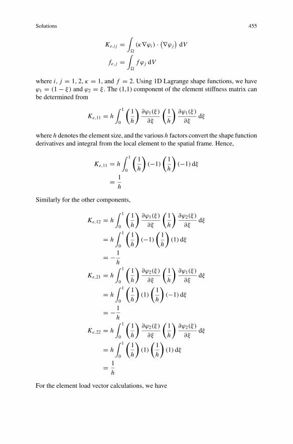
Solutions 455

Ke,i j =∫

�

(κ∇ϕi ) · (∇ϕ j)dV

fe, j =∫

�

f ϕ j dV

where i, j = 1, 2, κ = 1, and f = 2. Using 1D Lagrange shape functions, we haveϕ1 = (1 − ξ) and ϕ2 = ξ . The (1,1) component of the element stiffness matrix canbe determined from

Ke,11 = h∫ 1

0

(1

h

)∂ϕ1(ξ)

∂ξ

(1

h

)∂ϕ1(ξ)

∂ξdξ

where h denotes the element size, and the various h factors convert the shape functionderivatives and integral from the local element to the spatial frame. Hence,

Ke,11 = h∫ 1

0

(1

h

)(−1)

(1

h

)(−1) dξ

= 1

h

Similarly for the other components,

Ke,12 = h∫ 1

0

(1

h

)∂ϕ1(ξ)

∂ξ

(1

h

)∂ϕ2(ξ)

∂ξdξ

= h∫ 1

0

(1

h

)(−1)

(1

h

)(1) dξ

= −1

h

Ke,21 = h∫ 1

0

(1

h

)∂ϕ2(ξ)

∂ξ

(1

h

)∂ϕ1(ξ)

∂ξdξ

= h∫ 1

0

(1

h

)(1)

(1

h

)(−1) dξ

= −1

h

Ke,22 = h∫ 1

0

(1

h

)∂ϕ2(ξ)

∂ξ

(1

h

)∂ϕ2(ξ)

∂ξdξ

= h∫ 1

0

(1

h

)(1)

(1

h

)(1) dξ

= 1

h

For the element load vector calculations, we have

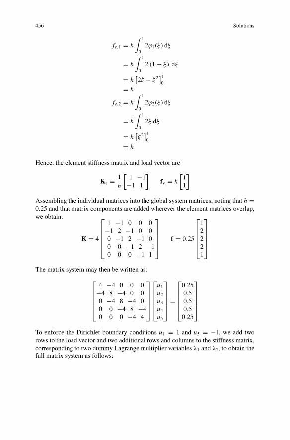
456 Solutions

fe,1 = h∫ 1

02ϕ1(ξ) dξ

= h∫ 1

02 (1 − ξ) dξ

= h[2ξ − ξ 2

]10

= h

fe,2 = h∫ 1

02ϕ2(ξ) dξ

= h∫ 1

02ξ dξ

= h[ξ 2]10

= h

Hence, the element stiffness matrix and load vector are

Ke = 1

h

[1 −1

−1 1

]fe = h

[11

]

Assembling the individual matrices into the global system matrices, noting that h =0.25 and that matrix components are added wherever the element matrices overlap,we obtain:

K = 4

⎡⎢⎢⎢⎢⎣

1 −1 0 0 0−1 2 −1 0 00 −1 2 −1 00 0 −1 2 −10 0 0 −1 1

⎤⎥⎥⎥⎥⎦ f = 0.25

⎡⎢⎢⎢⎢⎣

12221

⎤⎥⎥⎥⎥⎦

The matrix system may then be written as:

⎡⎢⎢⎢⎢⎣

4 −4 0 0 0−4 8 −4 0 00 −4 8 −4 00 0 −4 8 −40 0 0 −4 4

⎤⎥⎥⎥⎥⎦

⎡⎢⎢⎢⎢⎣

u1u2u3u4u5

⎤⎥⎥⎥⎥⎦ =

⎡⎢⎢⎢⎢⎣

0.250.50.50.50.25

⎤⎥⎥⎥⎥⎦

To enforce the Dirichlet boundary conditions u1 = 1 and u5 = −1, we add tworows to the load vector and two additional rows and columns to the stiffness matrix,corresponding to two dummy Lagrange multiplier variables λ1 and λ2, to obtain thefull matrix system as follows:

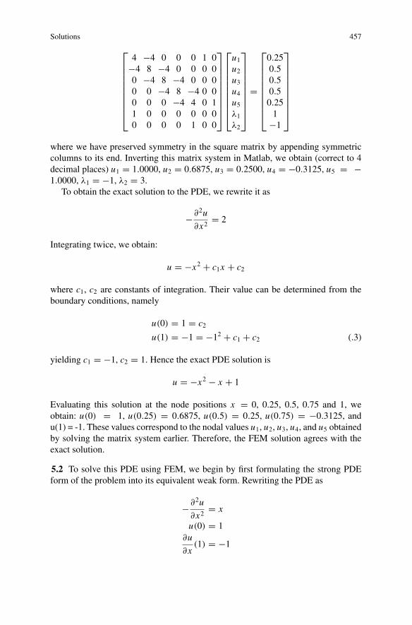
Solutions 457

⎡⎢⎢⎢⎢⎢⎢⎢⎢⎣

4 −4 0 0 0 1 0−4 8 −4 0 0 0 00 −4 8 −4 0 0 00 0 −4 8 −4 0 00 0 0 −4 4 0 11 0 0 0 0 0 00 0 0 0 1 0 0

⎤⎥⎥⎥⎥⎥⎥⎥⎥⎦

⎡⎢⎢⎢⎢⎢⎢⎢⎢⎣

u1u2u3u4u5λ1

λ2

⎤⎥⎥⎥⎥⎥⎥⎥⎥⎦

=

⎡⎢⎢⎢⎢⎢⎢⎢⎢⎣

0.250.50.50.50.251

−1

⎤⎥⎥⎥⎥⎥⎥⎥⎥⎦

where we have preserved symmetry in the square matrix by appending symmetriccolumns to its end. Inverting this matrix system in Matlab, we obtain (correct to 4decimal places) u1 = 1.0000, u2 = 0.6875, u3 = 0.2500, u4 = −0.3125, u5 = −1.0000, λ1 = −1, λ2 = 3.

To obtain the exact solution to the PDE, we rewrite it as

−∂2u

∂x2= 2

Integrating twice, we obtain:

u = −x2 + c1x + c2

where c1, c2 are constants of integration. Their value can be determined from theboundary conditions, namely

u(0) = 1 = c2u(1) = −1 = −12 + c1 + c2 (.3)

yielding c1 = −1, c2 = 1. Hence the exact PDE solution is

u = −x2 − x + 1

Evaluating this solution at the node positions x = 0, 0.25, 0.5, 0.75 and 1, weobtain: u(0) = 1, u(0.25) = 0.6875, u(0.5) = 0.25, u(0.75) = −0.3125, andu(1) = -1. These values correspond to the nodal values u1, u2, u3, u4, and u5 obtainedby solving the matrix system earlier. Therefore, the FEM solution agrees with theexact solution.

5.2 To solve this PDE using FEM, we begin by first formulating the strong PDEform of the problem into its equivalent weak form. Rewriting the PDE as

−∂2u

∂x2= x

u(0) = 1∂u

∂x(1) = −1

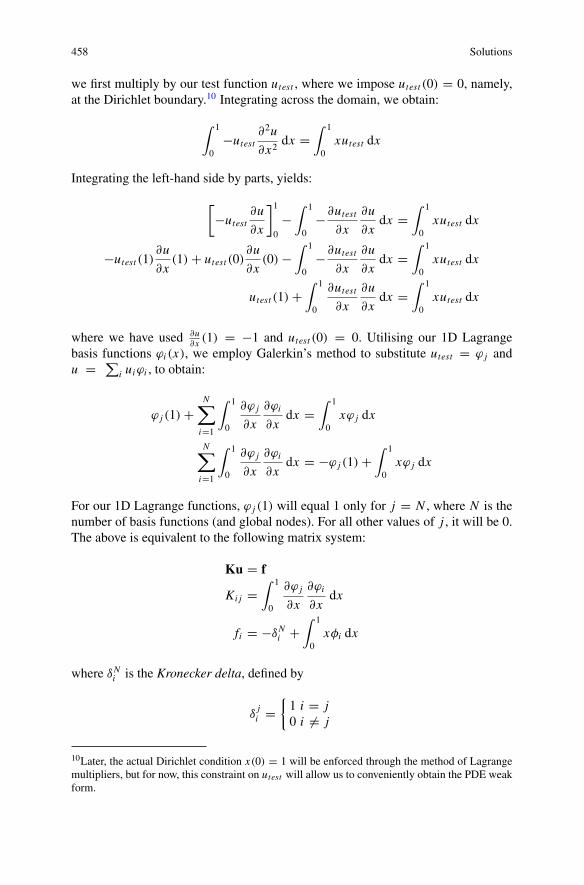
458 Solutions

we first multiply by our test function utest , where we impose utest (0) = 0, namely,at the Dirichlet boundary.10 Integrating across the domain, we obtain:

∫ 1

0−utest

∂2u

∂x2dx =

∫ 1

0xutest dx

Integrating the left-hand side by parts, yields:

[−utest

∂u

∂x

]10

−∫ 1

0−∂utest

∂x

∂u

∂xdx =

∫ 1

0xutest dx

−utest (1)∂u

∂x(1) + utest (0)

∂u

∂x(0) −

∫ 1

0−∂utest

∂x

∂u

∂xdx =

∫ 1

0xutest dx

utest (1) +∫ 1

0

∂utest∂x

∂u

∂xdx =

∫ 1

0xutest dx

where we have used ∂u∂x (1) = −1 and utest (0) = 0. Utilising our 1D Lagrange

basis functions ϕi (x), we employ Galerkin’s method to substitute utest = ϕ j andu = ∑

i uiϕi , to obtain:

ϕ j (1) +N∑i=1

∫ 1

0

∂ϕ j

∂x

∂ϕi

∂xdx =

∫ 1

0xϕ j dx

N∑i=1

∫ 1

0

∂ϕ j

∂x

∂ϕi

∂xdx = −ϕ j (1) +

∫ 1

0xϕ j dx

For our 1D Lagrange functions, ϕ j (1) will equal 1 only for j = N , where N is thenumber of basis functions (and global nodes). For all other values of j , it will be 0.The above is equivalent to the following matrix system:

Ku = f

Ki j =∫ 1

0

∂ϕ j

∂x

∂ϕi

∂xdx

fi = −δNi +∫ 1

0xφi dx

where δNi is the Kronecker delta, defined by

δji =

{1 i = j0 i �= j

10Later, the actual Dirichlet condition x(0) = 1 will be enforced through the method of Lagrangemultipliers, but for now, this constraint on utest will allow us to conveniently obtain the PDE weakform.

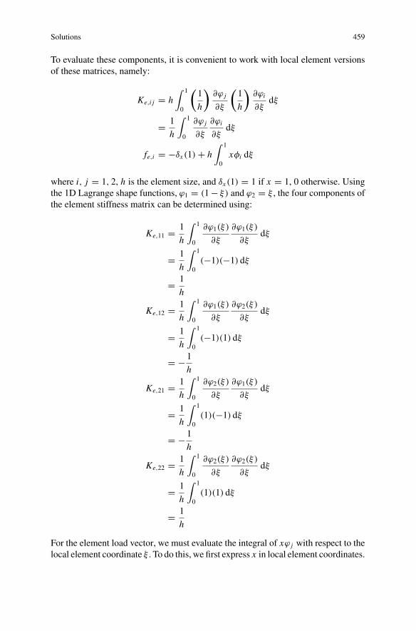
Solutions 459

To evaluate these components, it is convenient to work with local element versionsof these matrices, namely:

Ke,i j = h∫ 1

0

(1

h

)∂ϕ j

∂ξ

(1

h

)∂ϕi

∂ξdξ

= 1

h

∫ 1

0

∂ϕ j

∂ξ

∂ϕi

∂ξdξ

fe,i = −δx (1) + h∫ 1

0xφi dξ

where i, j = 1, 2, h is the element size, and δx (1) = 1 if x = 1, 0 otherwise. Usingthe 1D Lagrange shape functions, ϕ1 = (1− ξ) and ϕ2 = ξ , the four components ofthe element stiffness matrix can be determined using:

Ke,11 = 1

h

∫ 1

0

∂ϕ1(ξ)

∂ξ

∂ϕ1(ξ)

∂ξdξ

= 1

h

∫ 1

0(−1)(−1) dξ

= 1

h

Ke,12 = 1

h

∫ 1

0

∂ϕ1(ξ)

∂ξ

∂ϕ2(ξ)

∂ξdξ

= 1

h

∫ 1

0(−1)(1) dξ

= −1

h

Ke,21 = 1

h

∫ 1

0

∂ϕ2(ξ)

∂ξ

∂ϕ1(ξ)

∂ξdξ

= 1

h

∫ 1

0(1)(−1) dξ

= −1

h

Ke,22 = 1

h

∫ 1

0

∂ϕ2(ξ)

∂ξ

∂ϕ2(ξ)

∂ξdξ

= 1

h

∫ 1

0(1)(1) dξ

= 1

h

For the element load vector, we must evaluate the integral of xϕ j with respect to thelocal element coordinate ξ . To do this, we first express x in local element coordinates.

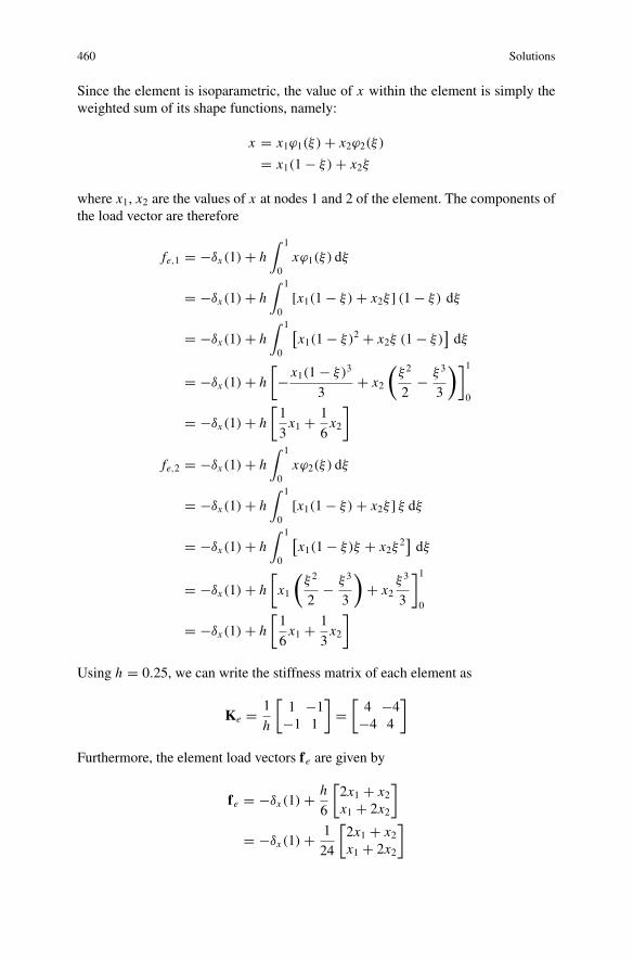
460 Solutions

Since the element is isoparametric, the value of x within the element is simply theweighted sum of its shape functions, namely:

x = x1ϕ1(ξ) + x2ϕ2(ξ)

= x1(1 − ξ) + x2ξ

where x1, x2 are the values of x at nodes 1 and 2 of the element. The components ofthe load vector are therefore

fe,1 = −δx (1) + h∫ 1

0xϕ1(ξ) dξ

= −δx (1) + h∫ 1

0[x1(1 − ξ) + x2ξ ] (1 − ξ) dξ

= −δx (1) + h∫ 1

0

[x1(1 − ξ)2 + x2ξ (1 − ξ)

]dξ

= −δx (1) + h

[− x1(1 − ξ)3

3+ x2

(ξ 2

2− ξ 3

3

)]10

= −δx (1) + h

[1

3x1 + 1

6x2

]

fe,2 = −δx (1) + h∫ 1

0xϕ2(ξ) dξ

= −δx (1) + h∫ 1

0[x1(1 − ξ) + x2ξ ] ξ dξ

= −δx (1) + h∫ 1

0

[x1(1 − ξ)ξ + x2ξ

2]dξ

= −δx (1) + h

[x1

(ξ 2

2− ξ 3

3

)+ x2

ξ 3

3

]10

= −δx (1) + h

[1

6x1 + 1

3x2

]

Using h = 0.25, we can write the stiffness matrix of each element as

Ke = 1

h

[1 −1

−1 1

]=

[4 −4

−4 4

]

Furthermore, the element load vectors fe are given by

fe = −δx (1) + h

6

[2x1 + x2x1 + 2x2

]

= −δx (1) + 1

24

[2x1 + x2x1 + 2x2

]

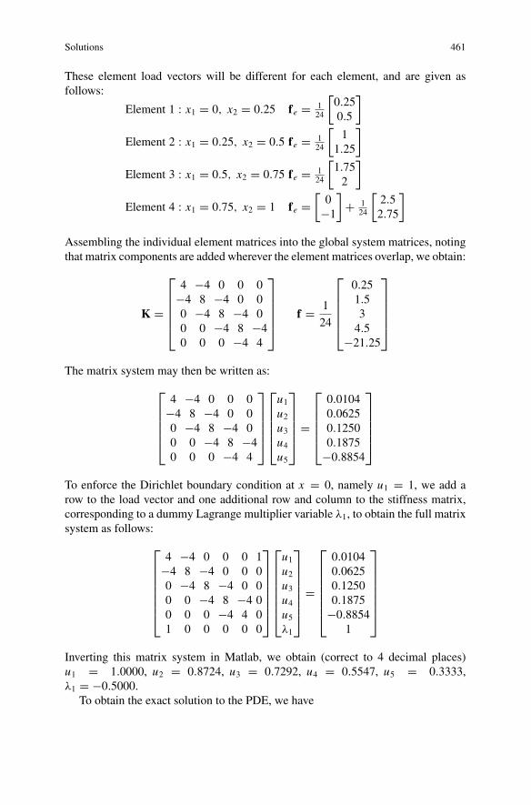
Solutions 461

These element load vectors will be different for each element, and are given asfollows:

Element 1 : x1 = 0, x2 = 0.25 fe = 124

[0.250.5

]

Element 2 : x1 = 0.25, x2 = 0.5 fe = 124

[1

1.25

]

Element 3 : x1 = 0.5, x2 = 0.75 fe = 124

[1.752

]

Element 4 : x1 = 0.75, x2 = 1 fe =[0

−1

]+ 1

24

[2.52.75

]

Assembling the individual element matrices into the global system matrices, notingthat matrix components are added wherever the element matrices overlap, we obtain:

K =

⎡⎢⎢⎢⎢⎣

4 −4 0 0 0−4 8 −4 0 00 −4 8 −4 00 0 −4 8 −40 0 0 −4 4

⎤⎥⎥⎥⎥⎦ f = 1

24

⎡⎢⎢⎢⎢⎣

0.251.534.5

−21.25

⎤⎥⎥⎥⎥⎦

The matrix system may then be written as:

⎡⎢⎢⎢⎢⎣

4 −4 0 0 0−4 8 −4 0 00 −4 8 −4 00 0 −4 8 −40 0 0 −4 4

⎤⎥⎥⎥⎥⎦

⎡⎢⎢⎢⎢⎣

u1u2u3u4u5

⎤⎥⎥⎥⎥⎦ =

⎡⎢⎢⎢⎢⎣

0.01040.06250.12500.1875

−0.8854

⎤⎥⎥⎥⎥⎦

To enforce the Dirichlet boundary condition at x = 0, namely u1 = 1, we add arow to the load vector and one additional row and column to the stiffness matrix,corresponding to a dummy Lagrange multiplier variable λ1, to obtain the full matrixsystem as follows:

⎡⎢⎢⎢⎢⎢⎢⎣

4 −4 0 0 0 1−4 8 −4 0 0 00 −4 8 −4 0 00 0 −4 8 −4 00 0 0 −4 4 01 0 0 0 0 0

⎤⎥⎥⎥⎥⎥⎥⎦

⎡⎢⎢⎢⎢⎢⎢⎣

u1u2u3u4u5λ1

⎤⎥⎥⎥⎥⎥⎥⎦

=

⎡⎢⎢⎢⎢⎢⎢⎣

0.01040.06250.12500.1875

−0.88541

⎤⎥⎥⎥⎥⎥⎥⎦

Inverting this matrix system in Matlab, we obtain (correct to 4 decimal places)u1 = 1.0000, u2 = 0.8724, u3 = 0.7292, u4 = 0.5547, u5 = 0.3333,λ1 = −0.5000.

To obtain the exact solution to the PDE, we have

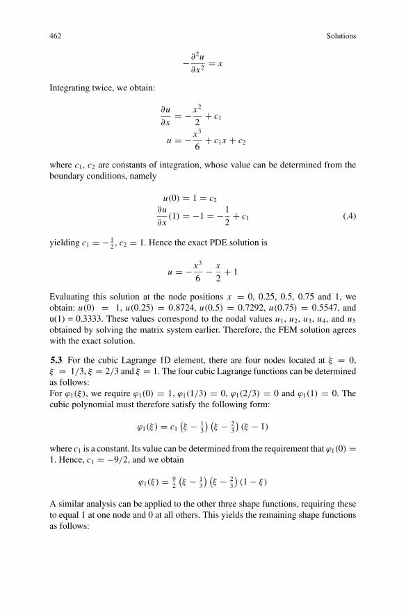
462 Solutions

−∂2u

∂x2= x

Integrating twice, we obtain:

∂u

∂x= − x2

2+ c1

u = − x3

6+ c1x + c2

where c1, c2 are constants of integration, whose value can be determined from theboundary conditions, namely

u(0) = 1 = c2∂u

∂x(1) = −1 = −1

2+ c1 (.4)

yielding c1 = − 12 , c2 = 1. Hence the exact PDE solution is

u = − x3

6− x

2+ 1

Evaluating this solution at the node positions x = 0, 0.25, 0.5, 0.75 and 1, weobtain: u(0) = 1, u(0.25) = 0.8724, u(0.5) = 0.7292, u(0.75) = 0.5547, andu(1) = 0.3333. These values correspond to the nodal values u1, u2, u3, u4, and u5obtained by solving the matrix system earlier. Therefore, the FEM solution agreeswith the exact solution.

5.3 For the cubic Lagrange 1D element, there are four nodes located at ξ = 0,ξ = 1/3, ξ = 2/3 and ξ = 1. The four cubic Lagrange functions can be determinedas follows:For ϕ1(ξ), we require ϕ1(0) = 1, ϕ1(1/3) = 0, ϕ1(2/3) = 0 and ϕ1(1) = 0. Thecubic polynomial must therefore satisfy the following form:

ϕ1(ξ) = c1(ξ − 1

3

) (ξ − 2

3

)(ξ − 1)

where c1 is a constant. Its value can be determined from the requirement that ϕ1(0) =1. Hence, c1 = −9/2, and we obtain

ϕ1(ξ) = 92

(ξ − 1

3

) (ξ − 2

3

)(1 − ξ)

A similar analysis can be applied to the other three shape functions, requiring theseto equal 1 at one node and 0 at all others. This yields the remaining shape functionsas follows:

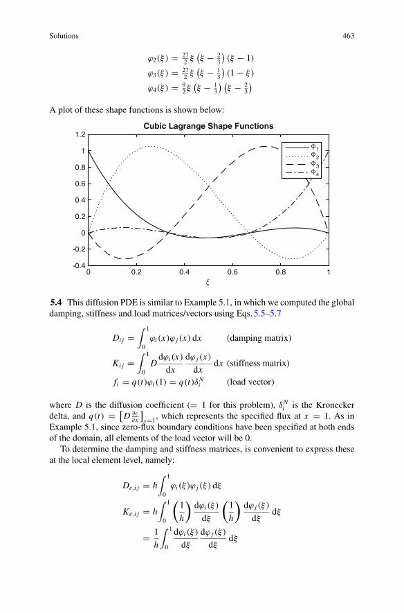
Solutions 463

ϕ2(ξ) = 272 ξ

(ξ − 2

3

)(ξ − 1)

ϕ3(ξ) = 272 ξ

(ξ − 1

3

)(1 − ξ)

ϕ4(ξ) = 92ξ

(ξ − 1

3

) (ξ − 2

3

)

A plot of these shape functions is shown below:

0 0.2 0.4 0.6 0.8 1-0.4

-0.2

0

0.2

0.4

0.6

0.8

1

1.2Cubic Lagrange Shape Functions

1

2

3

4

5.4 This diffusion PDE is similar to Example 5.1, in which we computed the globaldamping, stiffness and load matrices/vectors using Eqs. 5.5–5.7

Di j =∫ 1

0ϕi (x)ϕ j (x) dx (damping matrix)

Ki j =∫ 1

0Ddϕi (x)

dx

dϕ j (x)

dxdx (stiffness matrix)

fi = q(t)ϕi (1) = q(t)δNi (load vector)

where D is the diffusion coefficient (= 1 for this problem), δNi is the Kroneckerdelta, and q(t) = [

D ∂c∂x

]x=1

, which represents the specified flux at x = 1. As inExample 5.1, since zero-flux boundary conditions have been specified at both endsof the domain, all elements of the load vector will be 0.

To determine the damping and stiffness matrices, is convenient to express theseat the local element level, namely:

De,i j = h∫ 1

0ϕi (ξ)ϕ j (ξ) dξ

Ke,i j = h∫ 1

0

(1

h

)dϕi (ξ)

dξ

(1

h

)dϕ j (ξ)

dξdξ

= 1

h

∫ 1

0

dϕi (ξ)

dξ

dϕ j (ξ)

dξdξ

http://dx.doi.org/10.1007/978-3-642-54801-7_5

http://dx.doi.org/10.1007/978-3-642-54801-7_5

http://dx.doi.org/10.1007/978-3-642-54801-7_5

http://dx.doi.org/10.1007/978-3-642-54801-7_5

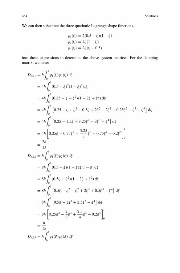
464 Solutions

We can then substitute the three quadratic Lagrange shape functions,

ϕ1(ξ) = 2(0.5 − ξ)(1 − ξ)

ϕ2(ξ) = 4ξ(1 − ξ)

ϕ3(ξ) = 2ξ(ξ − 0.5)

into these expressions to determine the above system matrices. For the dampingmatrix, we have:

De,11 = h∫ 1

0ϕ1(ξ)ϕ1(ξ) dξ

= 4h∫ 1

0(0.5 − ξ)2(1 − ξ)2 dξ

= 4h∫ 1

0(0.25 − ξ + ξ 2)(1 − 2ξ + ξ 2) dξ

= 4h∫ 1

0

[0.25 − ξ + ξ 2 − 0.5ξ + 2ξ 2 − 2ξ 3 + 0.25ξ 2 − ξ 3 + ξ 4] dξ

= 4h∫ 1

0

[0.25 − 1.5ξ + 3.25ξ 2 − 3ξ 3 + ξ 4] dξ

= 4h

[0.25ξ − 0.75ξ 2 + 3.25

3ξ 3 − 0.75ξ 4 + 0.2ξ 5

]10

= 2h

15

De,12 = h∫ 1

0ϕ1(ξ)ϕ2(ξ) dξ

= 8h∫ 1

0(0.5 − ξ)(1 − ξ)ξ(1 − ξ) dξ

= 8h∫ 1

0(0.5ξ − ξ 2)(1 − 2ξ + ξ 2) dξ

= 8h∫ 1

0

[0.5ξ − ξ 2 − ξ 2 + 2ξ 3 + 0.5ξ 3 − ξ 4

]dξ

= 8h∫ 1

0

[0.5ξ − 2ξ 2 + 2.5ξ 3 − ξ 4

]dξ

= 8h

[0.25ξ 2 − 2

3ξ 3 + 2.5

4ξ 4 − 0.2ξ 5

]10

= h

15

De,13 = h∫ 1

0ϕ1(ξ)ϕ3(ξ) dξ

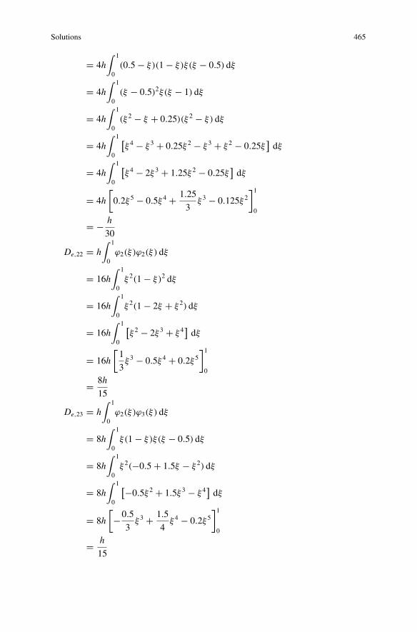
Solutions 465

= 4h∫ 1

0(0.5 − ξ)(1 − ξ)ξ(ξ − 0.5) dξ

= 4h∫ 1

0(ξ − 0.5)2ξ(ξ − 1) dξ

= 4h∫ 1

0(ξ 2 − ξ + 0.25)(ξ 2 − ξ) dξ

= 4h∫ 1

0

[ξ 4 − ξ 3 + 0.25ξ 2 − ξ 3 + ξ 2 − 0.25ξ

]dξ

= 4h∫ 1

0

[ξ 4 − 2ξ 3 + 1.25ξ 2 − 0.25ξ

]dξ

= 4h

[0.2ξ 5 − 0.5ξ 4 + 1.25

3ξ 3 − 0.125ξ 2

]10

= − h

30

De,22 = h∫ 1

0ϕ2(ξ)ϕ2(ξ) dξ

= 16h∫ 1

0ξ 2(1 − ξ)2 dξ

= 16h∫ 1

0ξ 2(1 − 2ξ + ξ 2) dξ

= 16h∫ 1

0

[ξ 2 − 2ξ 3 + ξ 4] dξ

= 16h

[1

3ξ 3 − 0.5ξ 4 + 0.2ξ 5

]10

= 8h

15

De,23 = h∫ 1

0ϕ2(ξ)ϕ3(ξ) dξ

= 8h∫ 1

0ξ(1 − ξ)ξ(ξ − 0.5) dξ

= 8h∫ 1

0ξ 2(−0.5 + 1.5ξ − ξ 2) dξ

= 8h∫ 1

0

[−0.5ξ 2 + 1.5ξ 3 − ξ 4]dξ

= 8h

[−0.5

3ξ 3 + 1.5

4ξ 4 − 0.2ξ 5

]10

= h

15

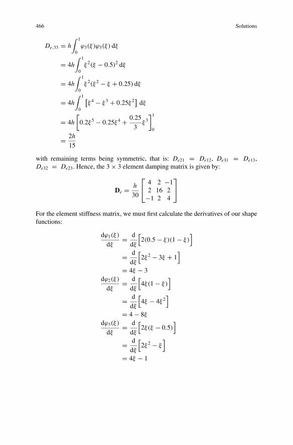
466 Solutions

De,33 = h∫ 1

0ϕ3(ξ)ϕ3(ξ) dξ

= 4h∫ 1

0ξ 2(ξ − 0.5)2 dξ

= 4h∫ 1

0ξ 2(ξ 2 − ξ + 0.25) dξ

= 4h∫ 1

0

[ξ 4 − ξ 3 + 0.25ξ 2

]dξ

= 4h

[0.2ξ 5 − 0.25ξ 4 + 0.25

3ξ 3

]10

= 2h

15

with remaining terms being symmetric, that is: De21 = De12, De31 = De13,De32 = De23. Hence, the 3 × 3 element damping matrix is given by:

De = h

30

⎡⎣ 4 2 −1

2 16 2−1 2 4

⎤⎦

For the element stiffness matrix, we must first calculate the derivatives of our shapefunctions:

dϕ1(ξ)

dξ= d

dξ

[2(0.5 − ξ)(1 − ξ)

]

= d

dξ

[2ξ 2 − 3ξ + 1

]

= 4ξ − 3dϕ2(ξ)

dξ= d

dξ

[4ξ(1 − ξ)

]

= d

dξ

[4ξ − 4ξ 2

]

= 4 − 8ξdϕ3(ξ)

dξ= d

dξ

[2ξ(ξ − 0.5)

]

= d

dξ

[2ξ 2 − ξ

]

= 4ξ − 1

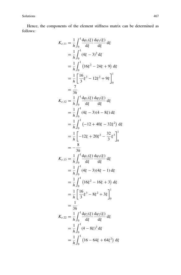
Solutions 467

Hence, the components of the element stiffness matrix can be determined asfollows:

Ke,11 = 1

h

∫ 1

0

dϕ1(ξ)

dξ

dϕ1(ξ)

dξdξ

= 1

h

∫ 1

0(4ξ − 3)2 dξ

= 1

h

∫ 1

0

(16ξ 2 − 24ξ + 9

)dξ

= 1

h

[16

3ξ 3 − 12ξ 2 + 9ξ

]10

= 7

3h

Ke,12 = 1

h

∫ 1

0

dϕ1(ξ)

dξ

dϕ2(ξ)

dξdξ

= 1

h

∫ 1

0(4ξ − 3)(4 − 8ξ) dξ

= 1

h

∫ 1

0

(−12 + 40ξ − 32ξ 2)dξ

= 1

h

[−12ξ + 20ξ 2 − 32

3ξ 3

]10

= − 8

3h

Ke,13 = 1

h

∫ 1

0

dϕ1(ξ)

dξ

dϕ3(ξ)

dξdξ

= 1

h

∫ 1

0(4ξ − 3)(4ξ − 1) dξ

= 1

h

∫ 1

0

(16ξ 2 − 16ξ + 3

)dξ

= 1

h

[16

3ξ 3 − 8ξ 2 + 3ξ

]10

= 1

3h

Ke,22 = 1

h

∫ 1

0

dϕ2(ξ)

dξ

dϕ2(ξ)

dξdξ

= 1

h

∫ 1

0(4 − 8ξ)2 dξ

= 1

h

∫ 1

0

(16 − 64ξ + 64ξ 2) dξ

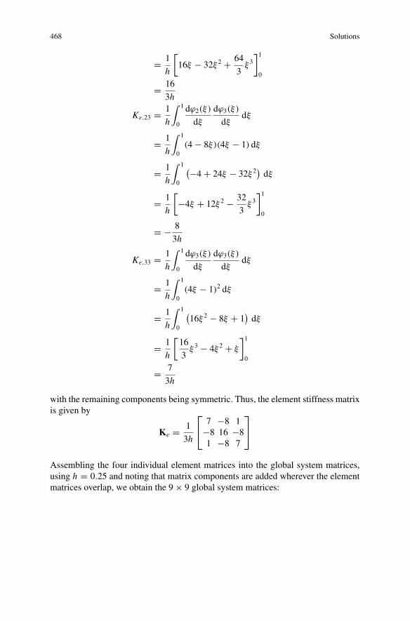
468 Solutions

= 1

h

[16ξ − 32ξ 2 + 64

3ξ 3

]10

= 16

3h

Ke,23 = 1

h

∫ 1

0

dϕ2(ξ)

dξ

dϕ3(ξ)

dξdξ

= 1

h

∫ 1

0(4 − 8ξ)(4ξ − 1) dξ

= 1

h

∫ 1

0

(−4 + 24ξ − 32ξ 2)dξ

= 1

h

[−4ξ + 12ξ 2 − 32

3ξ 3

]10

= − 8

3h

Ke,33 = 1

h

∫ 1

0

dϕ3(ξ)

dξ

dϕ3(ξ)

dξdξ

= 1

h

∫ 1

0(4ξ − 1)2 dξ

= 1

h

∫ 1

0

(16ξ 2 − 8ξ + 1

)dξ

= 1

h

[16

3ξ 3 − 4ξ 2 + ξ

]10

= 7

3h

with the remaining components being symmetric. Thus, the element stiffness matrixis given by

Ke = 1

3h

⎡⎣ 7 −8 1

−8 16 −81 −8 7

⎤⎦

Assembling the four individual element matrices into the global system matrices,using h = 0.25 and noting that matrix components are added wherever the elementmatrices overlap, we obtain the 9 × 9 global system matrices:

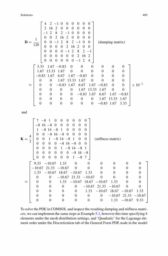
Solutions 469

D = 1

120

⎡⎢⎢⎢⎢⎢⎢⎢⎢⎢⎢⎢⎢⎣

4 2 −1 0 0 0 0 0 02 16 2 0 0 0 0 0 0

−1 2 8 2 −1 0 0 0 00 0 2 16 2 0 0 0 00 0 −1 2 8 2 −1 0 00 0 0 0 2 16 2 0 00 0 0 0 −1 2 8 2 −10 0 0 0 0 0 2 16 20 0 0 0 0 0 −1 2 4

⎤⎥⎥⎥⎥⎥⎥⎥⎥⎥⎥⎥⎥⎦

(damping matrix)

≈

⎡⎢⎢⎢⎢⎢⎢⎢⎢⎢⎢⎢⎢⎣

3.33 1.67 −0.83 0 0 0 0 0 01.67 13.33 1.67 0 0 0 0 0 0

−0.83 1.67 6.67 1.67 −0.83 0 0 0 00 0 1.67 13.33 1.67 0 0 0 00 0 −0.83 1.67 6.67 1.67 −0.83 0 00 0 0 0 1.67 13.33 1.67 0 00 0 0 0 −0.83 1.67 6.67 1.67 −0.830 0 0 0 0 0 1.67 13.33 1.670 0 0 0 0 0 −0.83 1.67 3.33

⎤⎥⎥⎥⎥⎥⎥⎥⎥⎥⎥⎥⎥⎦

× 10−2

and

K = 4

3

⎡⎢⎢⎢⎢⎢⎢⎢⎢⎢⎢⎢⎢⎣

7 −8 1 0 0 0 0 0 0−8 16 −8 0 0 0 0 0 01 −8 14 −8 1 0 0 0 00 0 −8 16 −8 0 0 0 00 0 1 −8 14 −8 1 0 00 0 0 0 −8 16 −8 0 00 0 0 0 1 −8 14 −8 10 0 0 0 0 0 −8 16 −80 0 0 0 0 0 1 −8 7

⎤⎥⎥⎥⎥⎥⎥⎥⎥⎥⎥⎥⎥⎦

(stiffness matrix)

≈

⎡⎢⎢⎢⎢⎢⎢⎢⎢⎢⎢⎢⎢⎣

9.33 −10.67 1.33 0 0 0 0 0 0−10.67 21.33 −10.67 0 0 0 0 0 01.33 −10.67 18.67 −10.67 1.33 0 0 0 00 0 −10.67 21.33 −10.67 0 0 0 00 0 1.33 −10.67 18.67 −10.67 1.33 0 00 0 0 0 −10.67 21.33 −10.67 0 00 0 0 0 1.33 −10.67 18.67 −10.67 1.330 0 0 0 0 0 −10.67 21.33 −10.670 0 0 0 0 0 1.33 −10.67 9.33

⎤⎥⎥⎥⎥⎥⎥⎥⎥⎥⎥⎥⎥⎦

To solve the PDE in COMSOL and inspect the resulting damping and stiffness matri-ces, we can implement the same steps as Example 5.1, however this time specifying 4elements under the mesh distribution settings, and ‘Quadratic’ for the Lagrange ele-ment order under the Discretization tab of the General Form PDE node in the model

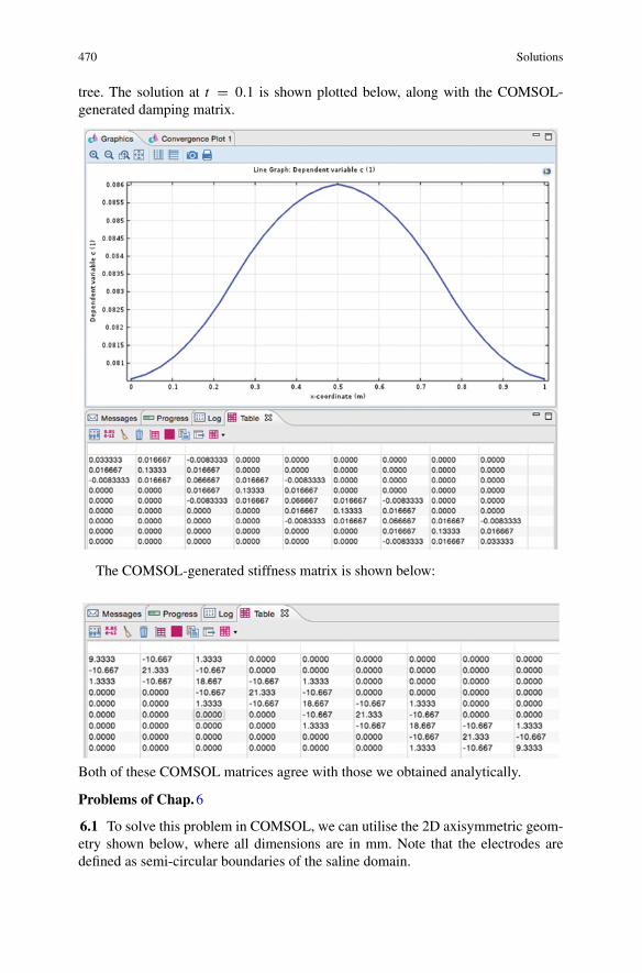
http://dx.doi.org/10.1007/978-3-642-54801-7_5

470 Solutions

tree. The solution at t = 0.1 is shown plotted below, along with the COMSOL-generated damping matrix.

The COMSOL-generated stiffness matrix is shown below:

Both of these COMSOL matrices agree with those we obtained analytically.

Problems of Chap.6

6.1 To solve this problem in COMSOL, we can utilise the 2D axisymmetric geom-etry shown below, where all dimensions are in mm. Note that the electrodes aredefined as semi-circular boundaries of the saline domain.

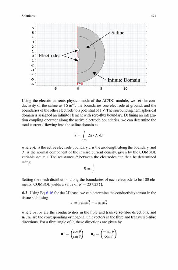
http://dx.doi.org/10.1007/978-3-642-54801-7_6

Solutions 471

Using the electric currents physics mode of the AC/DC module, we set the con-ductivity of the saline as 1Sm–1, the boundaries one electrode at ground, and theboundaries of the other electrode to a potential of 1V. The surrounding hemisphericaldomain is assigned an infinite element with zero-flux boundary. Defining an integra-tion coupling operator along the active electrode boundaries, we can determine thetotal current i flowing into the saline domain as

i =∫Ae

2πr Jn ds

where Ae is the active electrode boundary, s is the arc-length along the boundary, andJn is the normal component of the inward current density, given by the COMSOLvariable ec.nJ. The resistance R between the electrodes can then be determinedusing

R = 1

i

Setting the mesh distribution along the boundaries of each electrode to be 100 ele-ments, COMSOL yields a value of R = 237.23�.

6.2 Using Eq.6.16 for the 2D case, we can determine the conductivity tensor in thetissue slab using

σ = σ1n1nT1 + σ2n2nT

2

where σ1, σ2 are the conductivities in the fibre and transverse-fibre directions, andn1, n2 are the corresponding orthogonal unit vectors in the fibre and transverse-fibredirections. For a fibre angle of θ , these directions are given by

n1 =(cos θ

sin θ

)n2 =

(− sin θ

cos θ

)

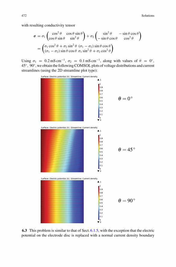
http://dx.doi.org/10.1007/978-3-642-54801-7_6

472 Solutions

with resulting conductivity tensor

σ = σ1

(cos2 θ cos θ sin θ

cos θ sin θ sin2 θ

)+ σ2

(sin2 θ − sin θ cos θ

− sin θ cos θ cos2 θ

)

=(

σ1 cos2 θ + σ2 sin2 θ (σ1 − σ2) sin θ cos θ

(σ1 − σ2) sin θ cos θ σ1 sin2 θ + σ2 cos2 θ

)

Using σ1 = 0.2mS cm−1, σ2 = 0.1mS cm−1, along with values of θ = 0◦,45◦, 90◦, we obtain the followingCOMSOLplots of voltage distributions and currentstreamlines (using the 2D streamline plot type):

6.3 This problem is similar to that of Sect. 6.1.5, with the exception that the electricpotential on the electrode disc is replaced with a normal current density boundary

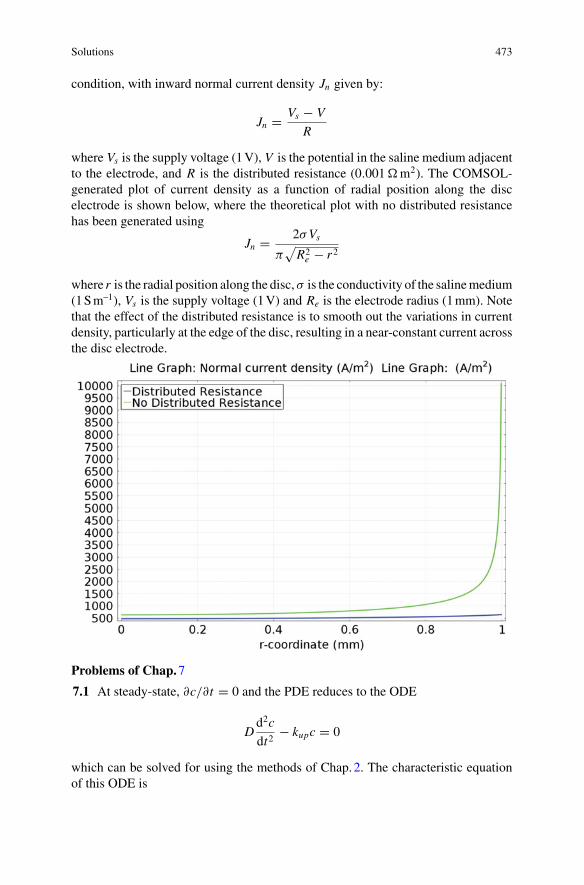
http://dx.doi.org/10.1007/978-3-642-54801-7_6

Solutions 473

condition, with inward normal current density Jn given by:

Jn = Vs − V

R

where Vs is the supply voltage (1V), V is the potential in the saline medium adjacentto the electrode, and R is the distributed resistance (0.001�m2). The COMSOL-generated plot of current density as a function of radial position along the discelectrode is shown below, where the theoretical plot with no distributed resistancehas been generated using

Jn = 2σVs

π√R2e − r2

where r is the radial position along the disc,σ is the conductivity of the salinemedium(1Sm–1), Vs is the supply voltage (1V) and Re is the electrode radius (1mm). Notethat the effect of the distributed resistance is to smooth out the variations in currentdensity, particularly at the edge of the disc, resulting in a near-constant current acrossthe disc electrode.

Problems of Chap.7

7.1 At steady-state, ∂c/∂t = 0 and the PDE reduces to the ODE

Dd2c

dt2− kupc = 0

which can be solved for using the methods of Chap.2. The characteristic equationof this ODE is

http://dx.doi.org/10.1007/978-3-642-54801-7_7

http://dx.doi.org/10.1007/978-3-642-54801-7_2

474 Solutions

Dm2 − kup = 0

∴ m = ±√kupD

Hence the solution is of the form

c(x) = C1ex√

kupD + C2e

−x√

kupD

where C1, C2 are constants which can be determined from the boundary conditions.Specifically, when x = 0, c = C0. Hence

C0 = C1 + C2

Also, when x = dc, c = 0. Hence

0 = C1edc

√kupD + C2e

−dc

√kupD

Substituting C2 = C0 − C1 into the above, we have

C1edc

√kupD + (C0 − C1)e

−dc

√kupD = 0

C1edc

√kupD − C1e

−dc

√kupD = −C0e

−dc

√kupD

C1

[edc

√kupD − e−dc

√kupD

]= −C0e

−dc

√kupD

∴ C1 = C0e−dc

√kupD

e−dc

√kupD − edc

√kupD

and using C2 = C0 − C1, we also obtain

C2 = C0 − C0e−dc

√kupD

e−dc

√kupD − edc

√kupD

= C0

⎡⎣e−dc

√kupD − edc

√kupD

e−dc

√kupD − edc

√kupD

⎤⎦ − C0e

−dc

√kupD

e−dc

√kupD − edc

√kupD

= − C0edc

√kupD

e−dc

√kupD − edc

√kupD

Substituting these values of C1, C2 into the general solution form, we obtain

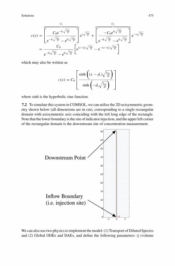
Solutions 475

c(x) =

C1︷︸︸︷⎡⎣ C0e

−dc

√kupD

e−dc

√kupD − edc

√kupD

⎤⎦ ex

√kupD +

C2︷︸︸︷⎡⎣ −C0e

dc

√kupD

e−dc

√kupD − edc

√kupD

⎤⎦ e−x

√kupD

= C0

e−dc

√kupD − edc

√kupD

[e(x−dc)

√kupD − e−(x−dc)

√kupD

]

which may also be written as

c(x) = C0

⎡⎢⎢⎣sinh

((x − dc)

√kupD

)

sinh

(−dc

√kupD

)⎤⎥⎥⎦

where sinh is the hyperbolic sine function.

7.2 To simulate this system in COMSOL,we can utilise the 2D axisymmetric geom-etry shown below (all dimensions are in cm), corresponding to a single rectangulardomain with axisymmetric axis coinciding with the left long edge of the rectangle.Note that the lower boundary is the site of indicator injection, and the upper left cornerof the rectangular domain is the downstream site of concentration measurement.

We can also use two physics to implement themodel: (1) Transport ofDiluted Speciesand (2) Global ODEs and DAEs, and define the following parameters: Q (volume

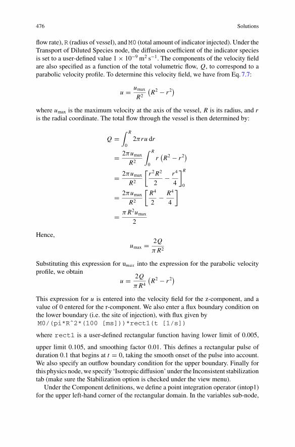
476 Solutions

flow rate), R (radius of vessel), and M0 (total amount of indicator injected). Under theTransport of Diluted Species node, the diffusion coefficient of the indicator speciesis set to a user-defined value 1 × 10−9 m2 s−1. The components of the velocity fieldare also specified as a function of the total volumetric flow, Q, to correspond to aparabolic velocity profile. To determine this velocity field, we have from Eq.7.7:

u = umax

R2

(R2 − r2

)

where umax is the maximum velocity at the axis of the vessel, R is its radius, and ris the radial coordinate. The total flow through the vessel is then determined by:

Q =∫ R

02πru dr

= 2πumax

R2

∫ R

0r(R2 − r2

)

= 2πumax

R2

[r2R2

2− r4

4

]R

0

= 2πumax

R2

[R4

2− R4

4

]

= πR2umax

2

Hence,

umax = 2Q

πR2

Substituting this expression for umax into the expression for the parabolic velocityprofile, we obtain

u = 2Q

πR4

(R2 − r2

)

This expression for u is entered into the velocity field for the z-component, and avalue of 0 entered for the r-component. We also enter a flux boundary condition onthe lower boundary (i.e. the site of injection), with flux given byM0/(pi*Rˆ2*(100 [ms]))*rect1(t [1/s])

where rect1 is a user-defined rectangular function having lower limit of 0.005,

upper limit 0.105, and smoothing factor 0.01. This defines a rectangular pulse ofduration 0.1 that begins at t = 0, taking the smooth onset of the pulse into account.We also specify an outflow boundary condition for the upper boundary. Finally forthis physics node,we specify ‘Isotropic diffusion’ under the Inconsistent stabilizationtab (make sure the Stabilization option is checked under the view menu).

Under the Component definitions, we define a point integration operator (intop1)for the upper left-hand corner of the rectangular domain. In the variables sub-node,

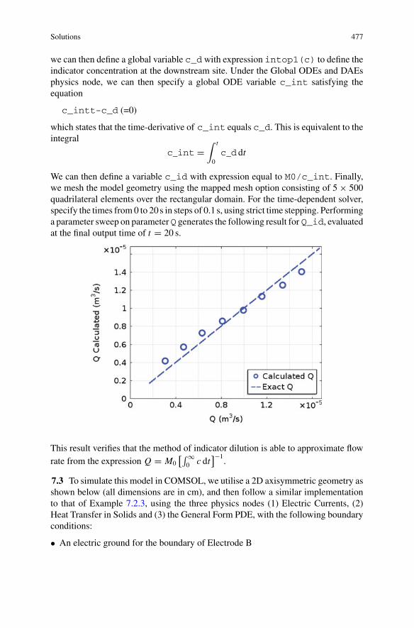
http://dx.doi.org/10.1007/978-3-642-54801-7_7

Solutions 477

we can then define a global variable c_dwith expression intop1(c) to define theindicator concentration at the downstream site. Under the Global ODEs and DAEsphysics node, we can then specify a global ODE variable c_int satisfying theequation

c_intt-c_d (=0)

which states that the time-derivative of c_int equals c_d. This is equivalent to theintegral

c_int =∫ t

0c_d dt

We can then define a variable c_id with expression equal to M0/c_int. Finally,we mesh the model geometry using the mapped mesh option consisting of 5 × 500quadrilateral elements over the rectangular domain. For the time-dependent solver,specify the times from 0 to 20s in steps of 0.1 s, using strict time stepping. Performinga parameter sweep on parameterQ generates the following result for Q_id, evaluatedat the final output time of t = 20 s.

This result verifies that the method of indicator dilution is able to approximate flowrate from the expression Q = M0

[∫∞0 c dt

]−1.

7.3 To simulate this model in COMSOL, we utilise a 2D axisymmetric geometry asshown below (all dimensions are in cm), and then follow a similar implementationto that of Example 7.2.3, using the three physics nodes (1) Electric Currents, (2)Heat Transfer in Solids and (3) the General Form PDE, with the following boundaryconditions:

• An electric ground for the boundary of Electrode B

http://dx.doi.org/10.1007/978-3-642-54801-7_7

478 Solutions

• An electric potential condition for Electrode boundary A (22 and 30V, imple-mented as a parametric sweep on a defined applied voltage parameter).

• Electric insulation on all other boundaries (except the axisymmetric axis, whichemploys a similar axisymmetric condition).

• A temperature boundary condition (37 ◦C for the outer boundaries of the tumour.• Thermal insulation on all other boundaries.

For the mesh, we set the general element size as ‘Extra fine’, and for the time-dependent solver, we use output times from 0 to 480s in steps of 1 s. Definingvariables and integration operators as in Example 7.2.3, we obtain the followingresult for the lesion volume for both 22 and 30V probe voltages.

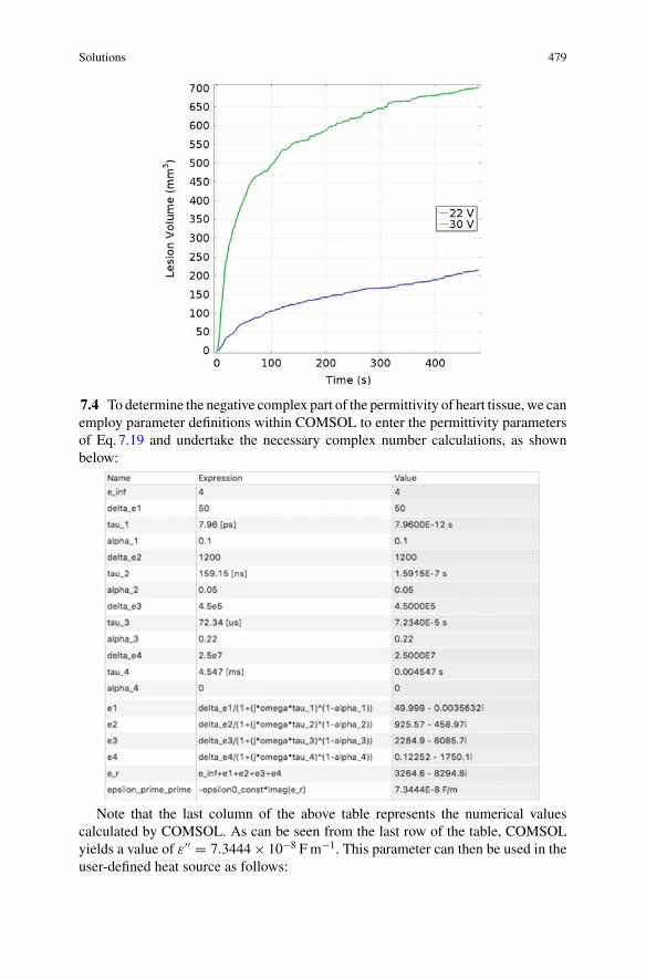
http://dx.doi.org/10.1007/978-3-642-54801-7_7

Solutions 479

7.4 To determine the negative complex part of the permittivity of heart tissue, we canemploy parameter definitions within COMSOL to enter the permittivity parametersof Eq.7.19 and undertake the necessary complex number calculations, as shownbelow:

Note that the last column of the above table represents the numerical valuescalculated by COMSOL. As can be seen from the last row of the table, COMSOLyields a value of ε′′ = 7.3444× 10−8 F m−1. This parameter can then be used in theuser-defined heat source as follows:

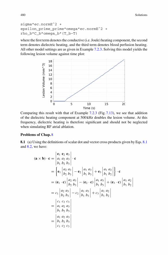
http://dx.doi.org/10.1007/978-3-642-54801-7_7

480 Solutions

sigma*ec.normEˆ2 +epsilon_prime_prime*omega*ec.normEˆ2 +rho_b*C_b*omega_b*(T_b-T)

where the first term denotes the conductive (i.e. Joule) heating component, the secondterm denotes dielectric heating, and the third term denotes blood perfusion heating.All other model settings are as given in Example 7.2.3. Solving this model yields thefollowing lesion volume against time plot:

Comparing this result with that of Example 7.2.3 (Fig. 7.13), we see that additionof the dielectric heating component at 500kHz doubles the lesion volume. At thisfrequency, dielectric heating is therefore significant and should not be neglectedwhen simulating RF atrial ablation.

Problems of Chap.8

8.1 (a) Using the definitions of scalar dot and vector cross products given by Eqs. 8.1and 8.2, we have:

(a × b) · c =∣∣∣∣∣∣e1 e2 e3a1 a2 a3b1 b2 b3

∣∣∣∣∣∣ · c

={e1

∣∣∣∣a2 a3b2 b3

∣∣∣∣ − e2

∣∣∣∣a1 a3b1 b3

∣∣∣∣ + e3

∣∣∣∣a1 a2b1 b2

∣∣∣∣}

· c

= (e1 · c)∣∣∣∣a2 a3b2 b3

∣∣∣∣ − (e2 · c)∣∣∣∣a1 a3b1 b3

∣∣∣∣ + (e3 · c)∣∣∣∣a1 a2b1 b2

∣∣∣∣= c1

∣∣∣∣a2 a3b2 b3

∣∣∣∣ − c2

∣∣∣∣a1 a3b1 b3

∣∣∣∣ + c3

∣∣∣∣a1 a2b1 b2

∣∣∣∣

=∣∣∣∣∣∣c1 c2 c3a1 a2 a3b1 b2 b3

∣∣∣∣∣∣

=∣∣∣∣∣∣a1 a2 a3b1 b2 b3c1 c2 c3

∣∣∣∣∣∣

http://dx.doi.org/10.1007/978-3-642-54801-7_7

http://dx.doi.org/10.1007/978-3-642-54801-7_7

http://dx.doi.org/10.1007/978-3-642-54801-7_7

http://dx.doi.org/10.1007/978-3-642-54801-7_8

http://dx.doi.org/10.1007/978-3-642-54801-7_8

http://dx.doi.org/10.1007/978-3-642-54801-7_8

Solutions 481

Expanding this determinant, we obtain:

∣∣∣∣∣∣a1 a2 a3b1 b2 b3c1 c2 c3

∣∣∣∣∣∣ = a1

∣∣∣∣ b2 b3c2 c3

∣∣∣∣ − a2

∣∣∣∣ b1 b3c1 c3

∣∣∣∣ + a3

∣∣∣∣ b1 b2c1 c2

∣∣∣∣= a1 (b2c3 − b3c2) − a2 (b1c3 − b3c1) + a3 (b1c2 − b2c1)

= a1b2c3 − a1b3c2 − a2b1c3 + a2b3c1 + a3b1c2 − a3b2c1= εi jkai b j ck

Hence,

(a × b) · c =∣∣∣∣∣∣a1 a2 a3b1 b2 b3c1 c2 c3

∣∣∣∣∣∣ = εi jkai b j ck

(b) We recall thatσHi j = 1

3σααδi j εHi j = 13εααδi j

and writing these hydrostatic tensors in terms of their components, we have:

σH =⎛⎝

13 (σ11 + σ22 + σ33) 0 0

0 13 (σ11 + σ22 + σ33) 0

0 0 13 (σ11 + σ22 + σ33)

⎞⎠

εH =⎛⎝

13 (ε11 + ε22 + ε33) 0 0

0 13 (ε11 + ε22 + ε33) 0

0 0 13 (ε11 + ε22 + ε33)

⎞⎠

For the deviatoric tensors, we have

σD = σ − σH εD = ε − εH

and therefore

σD =⎛⎝

13 (2σ11 − σ22 − σ33) σ12 σ13

σ2113 (−σ11 + 2σ22 − σ33) σ23

σ31 σ3213 (−σ11 − σ22 + 2σ33)

⎞⎠

εD =⎛⎝

13 (2ε11 − ε22 − ε33) ε12 ε13

ε2113 (−ε11 + 2ε22 − ε33) ε23

ε31 ε3213 (−ε11 − ε22 + 2ε33)

⎞⎠

In particular, we note that

trace(σD

) = 13 {2σ11 − σ22 − σ33 − σ11 + 2σ22 − σ33 − σ11 − σ22 + 2σ33} = 0

trace(εD) = 1

3 {2ε11 − ε22 − ε33 − ε11 + 2ε22 − ε33 − ε11 − ε22 + 2ε33} = 0

482 Solutions

Writing

σH =⎛⎝σH 0 0

0 σH 00 0 σH

⎞⎠ , εH =

⎛⎝εH 0 0

0 εH 00 0 εH

⎞⎠

withσH = 1

3 (σ11 + σ22 + σ33) , εH = 13 (ε11 + ε22 + ε33)

we have:σHi j ε

Di j = σH

11εD11 + σH

22εD22 + σH

33εD33 = σH trace

(εD

) = 0

andσDi j ε

Hi j = σD

11εH11 + σD

22εH22 + σD

33εH33 = εH trace

(σD

) = 0

Hence we have verified that σHi j ε

Di j = σD

i j εHi j = 0.

8.2 (a) For the simple shear deformation given, we have

u1 = λx2, u2 = 0

Therefore,

ε11 = ∂u1∂x1

= 0

ε12 = ε21 = 12

(∂u1∂x2

+ ∂u2∂x1

)= 1

2 (λ + 0) = λ

2

ε22 = ∂u2∂x2

= 0

and

E11 = 12

(∂u1∂x1

+ ∂u1∂x1

+ ∂u1∂x1

∂u1∂x1

)= 0

E12 = E21 = 12

(∂u1∂x2

+ ∂u2∂x1

+ ∂u1∂x2

∂u2∂x1

)= 1

2 (λ + 0 + λ · 0) = λ

2

E22 = 12

(∂u2∂x2

+ ∂u2∂x2

+ ∂u2∂x2

∂u2∂x2

)= 0

In matrix form, these strain tensors are

ε =(0 λ

2λ2 0

), E =

(0 λ

2λ2 0

)

Solutions 483

(b) For the uniform inflation deformation, we have

u1 = (R − 1)x1, u2 = (R − 1)x2

Therefore,

ε11 = ∂u1∂x1

= R − 1

ε12 = ε21 = 12

(∂u1∂x2

+ ∂u2∂x1

)= 0

ε22 = ∂u2∂x2

= R − 1

and

E11 = 12

(∂u1∂x1

+ ∂u1∂x1

+ ∂u1∂x1

∂u1∂x1

)= 1

2

(2R − 2 + (R − 1)2

)= 1

2 ((R − 1)(R + 1))

= 12

(R2 − 1

)

E12 = E21 = 12

(∂u1∂x2

+ ∂u2∂x1

+ ∂u1∂x2

∂u2∂x1

)= 0

E22 = 12

(∂u2∂x2

+ ∂u2∂x2

+ ∂u2∂x2

∂u2∂x2

)= 1

2

(2R − 2 + (R − 1)2

)= 1

2 ((R − 1)(R + 1))

= 12

(R2 − 1

)

In matrix form, these strain tensors are

ε =(R − 1 00 R − 1

), E =

( 12

(R2 − 1

)0

0 12

(R2 − 1

))

(c) In the case of rotation, a point originally at (x1, x2) is rotated to the new point(x1, x2) according to the rotation transformation:

(x1x2

)=

(cos θ − sin θ

sin θ cos θ

)(x1x2

)

Hence the displacements are given by

u1 = x1 cos θ − x2 sin θ − x1 = x2 (cos θ − 1) − x2 sin θ

u2 = x2 cos θ + x1 sin θ − x2 = x1 (cos θ − 1) + x1 sin θ

Therefore,

484 Solutions

ε11 = ∂u1∂x1

= cos θ − 1

ε12 = ε21 = 12

(∂u1∂x2

+ ∂u2∂x1

)= 1

2 (− sin θ + sin θ) = 0

ε22 = ∂u2∂x2

= cos θ − 1

and

E11 = 12

(∂u1∂x1

+ ∂u1∂x1

+ ∂u1∂x1

∂u1∂x1

)= 1

2

(2(cos θ − 1) + (cos θ − 1)2

)

= 12 ((cos θ − 1)(cos θ + 1)) = 1

2

(cos2 θ − 1

) = − 12 sin

2 θ

E12 = E21 = 12

(∂u1∂x2

+ ∂u2∂x1

+ ∂u1∂x2

∂u2∂x1

)= 1

2 (− sin θ + sin θ + − sin θ · sin θ)

= − 12 sin

2 θ

E22 = 12

(∂u2∂x2

+ ∂u2∂x2

+ ∂u2∂x2

∂u2∂x2

)== 1

2

(2(cos θ − 1) + (cos θ − 1)2

)

= 12 ((cos θ − 1)(cos θ + 1)) = 1

2

(cos2 θ − 1

) = − 12 sin

2 θ

In matrix form, these strain tensors are therefore given by

ε =(cos θ − 1 0

0 cos θ − 1

), E = 1

2

(− sin2 θ − sin2 θ

− sin2 θ − sin2 θ

)

8.3 (a) For an incompressible deformation, the volume of the spherical shell mustbe preserved. That is:

43π

(b3 − a3

) = 43π

(B3 − A3

)

Therefore,

b3 = a3 + B3 − A3

b = 3√a3 + B3 − A3

(b) For a particle in the myocardial wall initially located at a radial position of R,we can use a similar analysis as part a) to show that the volume of the shell betweenradial distances of A and R must be preserved. Hence, if this particle moves to a newradial position of r , then we must have

r = 3√a3 + R3 − A3

which corresponds to a radial displacementu(R) = r−R, withu1,u2,u3 componentsof

Solutions 485

u1 =( x1R

)u(R) = x1

R

(3√a3 + R3 − A3 − R

)= x1

(3

√1 + a3 − A3

R3− 1

)

u2 =( x2R

)u(R) = x2

R

(3√a3 + R3 − A3 − R

)= x2

(3

√1 + a3 − A3

R3− 1

)

u3 =( x3R

)u(R) = x3

R

(3√a3 + R3 − A3 − R

)= x3

(3

√1 + a3 − A3

R3− 1

)

where R =√x21 + x22 + x23 . For convenience, we let γ = 3

√1 + a3−A3

R3 − 1 and writethese displacement components as

u1 = γ x1, u2 = γ x2, u3 = γ x3

To determine the components of Cauchy strain, we need to determine the partialderivatives of these displacements with respect to x1, x2 and x3. These in turn requirethe following derivatives:

dγ

dR= 1

3

(1 + a3 − A3

R3

)− 23[

−3(a3 − A3

)R4

]

= −[a3 − A3

R4

](1 + a3 − A3

R3

)− 23

= −[(γ + 1)3 − 1

R

](γ + 1)−2

= − 1

R

[γ + 1 − 1

(γ + 1)2

]

∂R

∂x1= 1

2

(x21 + x22 + x23

)− 12 2x1 = x1

R∂R

∂x2= 1

2

(x21 + x22 + x23

)− 12 2x2 = x2

R∂R

∂x3= 1

2

(x21 + x22 + x23

)− 12 2x3 = x3

R

Hence, the derivatives of displacement u1 with respect to each of x1, x2, and x3 are:

∂u1∂x1

= γ + x1∂γ

∂x1= γ + x1

dγ

dR

∂R

∂x1= γ − x21

R2

[γ + 1 − 1

(γ + 1)2

]

∂u1∂x2

= x1∂γ

∂x2= x1

dγ

dR

∂R

∂x2= − x1x2

R2

[γ + 1 − 1

(γ + 1)2

]

486 Solutions

∂u1∂x3

= x1∂γ

∂x3= x1

dγ

dR

∂R

∂x3= − x1x3

R2

[γ + 1 − 1

(γ + 1)2

]

Again for convenience, we let β = γ + 1 − 1(γ+1)2 . The above derivatives then

become:∂u1∂x1

= γ − βx21R2

,∂u1∂x2

= −βx1x2R2

,∂u1∂x3

= −βx1x3R2

Similarly, we obtain the remaining derivatives of the other displacement terms as

∂u2∂x1

= −βx1x2R2

,∂u2∂x2

= γ − βx22R2

,∂u2∂x3

= −βx2x3R2

∂u3∂x1

= −βx1x3R2

,∂u2∂x3

= −βx2x3R2

,∂u3∂x3

= γ − βx23R2

The Cauchy strain is given by εi j = 12

(∂ui∂x j

+ ∂u j

∂xi

). Inserting the above derivatives,

we obtain its following matrix form:

ε =⎛⎜⎝

γ − βx21R2 − βx1x2

R2 − βx1x3R2

− βx1x2R2 γ − βx22

R2 − βx2x3R2

− βx1x3R2 − βx2x3

R2 γ − βx23R2

⎞⎟⎠

where, as indicated earlier, γ = 3

√1 + a3−A3

R3 − 1 and β = γ + 1 − 1(γ+1)2 .

8.4 (a) Since the skin thickness of the sample is small compared to its other dimen-sions, a 2D implementation in COMSOL is preferable, using the plane stress con-dition (i.e. there are no components of stress perpendicular to the plane). Since themodel is symmetric, we can implement only half of the geometry, employing a sym-metric boundary condition on the lower face. The following are key points regardingthis COMSOL implementation

• In the Solid Mechanics settings, specify a thickness of 1mm and the plane stress2D approximation mode.

• Specify a hyperelastic material employing the Mooney-Rivlin, two parametersmaterial model. Enter all user-defined material values as given.

• Specify a prescribed displacement boundary condition on the right boundary withonly a prescribed x-displacement of d, where d is a user-defined global modelparameter. Specify a symmetry boundary condition for the lower boundary a fixedconstraint boundary condition for the left boundary.

• Define an integration boundary operator, intop1, acting over the right boundary.Define a model variable F representing the applied force, given by the expres-sion 2*intop1(solid.Tax)*(1 [mm]). In this expression, Tax denotes aCOMSOL in-built variable for the x-component of traction, (1 [mm]) denotes

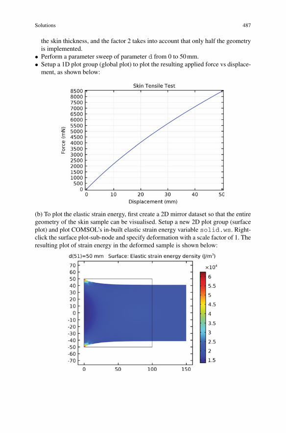
Solutions 487

the skin thickness, and the factor 2 takes into account that only half the geometryis implemented.

• Perform a parameter sweep of parameter d from 0 to 50mm.• Setup a 1D plot group (global plot) to plot the resulting applied force vs displace-ment, as shown below:

(b) To plot the elastic strain energy, first create a 2D mirror dataset so that the entiregeometry of the skin sample can be visualised. Setup a new 2D plot group (surfaceplot) and plot COMSOL’s in-built elastic strain energy variable solid.ws. Right-click the surface plot-sub-node and specify deformation with a scale factor of 1. Theresulting plot of strain energy in the deformed sample is shown below:

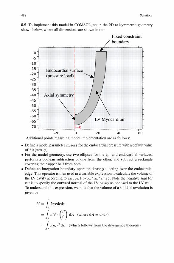
488 Solutions

8.5 To implement this model in COMSOL, setup the 2D axisymmetric geometryshown below, where all dimensions are shown in mm:

Additional points regarding model implementation are as follows:

• Define amodel parameter press for the endocardial pressure with a default valueof 50[mmHg].

• For the model geometry, use two ellipses for the epi and endocardial surfaces,perform a boolean subtraction of one from the other, and subtract a rectanglecovering their upper half from both.

• Define an integration boundary operator, intop1, acting over the endocardialedge. This operator is then used in a variable expression to calculate the volume ofthe LV cavity according to intop1(-pi*nr*rˆ2). Note the negative sign fornr is to specify the outward normal of the LV cavity as opposed to the LV wall.To understand this expression, we note that the volume of a solid of revolution isgiven by

V =∫A2πrdrdz

=∫Aπ∇ ·

(r2

0

)dA (where dA = drdz)

=∫Lπnrr

2 dL (which follows from the divergence theorem)

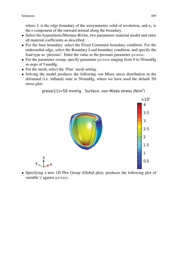
Solutions 489

where L is the edge boundary of the axisymmetric solid of revolution, and nr isthe r-component of the outward normal along the boundary.

• Select the hyperelastic/Mooney-Rivlin, two parameters material model and enterall material coefficients as described.

• For the base boundary, select the Fixed Constraint boundary condition. For theendocardial edge, select the Boundary Load boundary condition, and specify theload type as ‘pressure’. Enter the value as the pressure parameter press.

• For the parameter sweep, specify parameter press ranging from 0 to 50mmHgin steps of 5mmHg.

• For the mesh, select the ‘Fine’ mesh setting.• Solving the model produces the following von Mises stress distribution in thedeformed (i.e. inflated) state at 50mmHg, where we have used the default 3Dstress plot:

• Specifying a new 1D Plot Group (Global plot), produces the following plot ofvariable V against press:

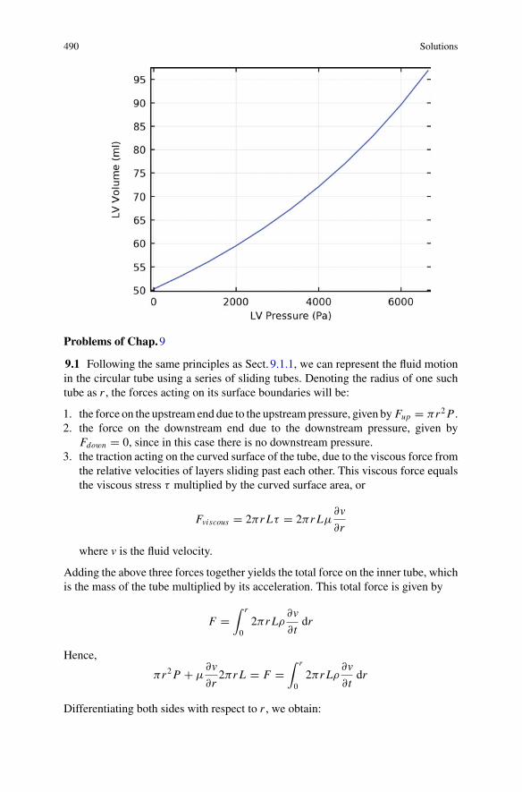
490 Solutions

Problems of Chap.9

9.1 Following the same principles as Sect. 9.1.1, we can represent the fluid motionin the circular tube using a series of sliding tubes. Denoting the radius of one suchtube as r , the forces acting on its surface boundaries will be:

1. the force on the upstream end due to the upstreampressure, given by Fup = πr2P .2. the force on the downstream end due to the downstream pressure, given by

Fdown = 0, since in this case there is no downstream pressure.3. the traction acting on the curved surface of the tube, due to the viscous force from

the relative velocities of layers sliding past each other. This viscous force equalsthe viscous stress τ multiplied by the curved surface area, or

Fviscous = 2πr Lτ = 2πr Lμ∂v

∂r

where v is the fluid velocity.

Adding the above three forces together yields the total force on the inner tube, whichis the mass of the tube multiplied by its acceleration. This total force is given by

F =∫ r

02πr Lρ

∂v

∂tdr

Hence,

πr2P + μ∂v

∂r2πr L = F =

∫ r

02πr Lρ

∂v

∂tdr

Differentiating both sides with respect to r , we obtain:

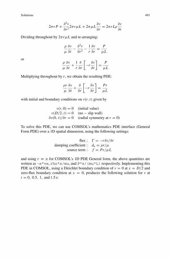
http://dx.doi.org/10.1007/978-3-642-54801-7_9

http://dx.doi.org/10.1007/978-3-642-54801-7_9

Solutions 491

2πr P + ∂2v

∂r22πrμL + 2πμL

∂v

∂r= 2πr Lρ

∂v

∂t

Dividing throughout by 2πrμL and re-arranging:

ρ

μ

∂v

∂t− ∂2v

∂r2− 1

r

∂v

∂r= P

μL

orρ

μ

∂v

∂t+ 1

r

∂

∂r

[−r

∂v

∂r

]= P

μL

Multiplying throughout by r , we obtain the resulting PDE:

ρr

μ

∂v

∂t+ ∂

∂r

[−r

∂v

∂r

]= Pr

μL

with initial and boundary conditions on v(r, t) given by

v(r, 0) = 0 (initial value)v(D/2, t) = 0 (no − slip wall)

∂v(0, t)/∂r = 0 (radial symmetry at r = 0)

To solve this PDE, we can use COMSOL’s mathematics PDE interface (GeneralForm PDE) over a 1D spatial dimension, using the following settings:

flux : � = −r∂v/∂rdamping coefficient : da = ρr/μ

source term : f = Pr/μL

and using r ≡ x for COMSOL’s 1D PDE General form, the above quantities arewritten as -x*vx, rho*x/mu, and P*x/(mu*L) respectively. Implementing thisPDE in COMSOL, using a Dirichlet boundary condition of v = 0 at x = D/2 andzero-flux boundary condition at x = 0, produces the following solution for v att = 0, 0.5, 1, and 1.5 s:

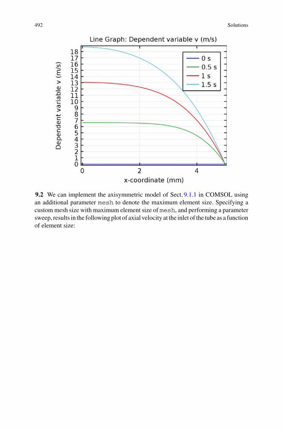
492 Solutions

9.2 We can implement the axisymmetric model of Sect. 9.1.1 in COMSOL usingan additional parameter mesh to denote the maximum element size. Specifying acustommesh size with maximum element size of mesh, and performing a parametersweep, results in the followingplot of axial velocity at the inlet of the tube as a functionof element size:

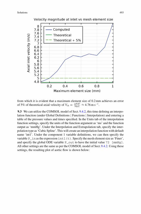
http://dx.doi.org/10.1007/978-3-642-54801-7_9

Solutions 493

from which it is evident that a maximum element size of 0.2mm achieves an errorof 5% of theoretical axial velocity of Vth = ΔPD2

16μL ≈ 4.76m s−1.

9.3 We can utilize the COMSOLmodel of Sect. 9.4.2, this time defining an interpo-lation function (under Global Definitions | Functions | Interpolation) and entering atable of the pressure values and times specified. In the Units tab of the interpolationfunction settings, specify the units of the function argument as ‘ms’ and the functionoutput as ‘mmHg’. Under the Interpolation and Extrapolation tab, specify the inter-polation type as ‘Cubic Spline’. Thiswill create an interpolation functionwith defaultname ‘int1’. Under the component 1 variable definitions, we can then specify thevariableP_in as the expressionint1(t). Specify themesh element size as ‘Finer’,and specify the global ODE variable P_out to have the initial value 72 [mmHg].All other settings are the same as per the COMSOLmodel of Sect. 9.4.2. Using thesesettings, the resulting plot of aortic flow is shown below:

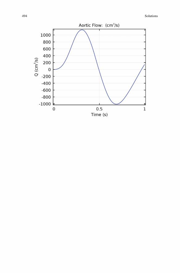
http://dx.doi.org/10.1007/978-3-642-54801-7_9

http://dx.doi.org/10.1007/978-3-642-54801-7_9

494 Solutions

Index

AAction Potential, 36, 42, 49, 151, 155, 217,

234, 379, 406Algebraic Equation (AE), 29–30Arrhenius Equation, 251Arrhenius, Svante, 251Axial Streaming, 330

model of, 330–339Axisymmetric Models, 128, 211–215, 239–

241, 244–247, 251–258, 302, 308–310, 314–321, 325–329, 340, 357,470, 475–477, 488–490, 492–493

BBackward Difference

backward difference operator, 83Newton’s backward difference formula,83

Backward Differentiation Formula (BDF),93–96, 98, 103, 427–430

coefficients, 95order selection, 95

Bacterial Growth, models of, 6, 23, 29–30Basis Functions, 159, 164–179, 183–190,

196, see also Shape Functions1D linear (witch’s hat), 164, 165, 167,170, 171, 174, 176

Beeler–Reuter Model, 100–102, 410–420Bidomain Equations, 216–217

COMSOL example (cardiac reentry),217–225

Bioheat Equation, 250–251, see also HeatTransfer

Blood Flow, 324–339hydraulic circuits, 37–42, 324–329, 340–341, 493

in a cylindrical vessel, 19–21, 306–310,340–341, 490–493

models of, 242–247, 314–321, 325–339non-Newtonian properties of, 329–330

Body Force, 274, 312, 323Boundary Conditions, 4–6, 120–123, 133,

160, 161, 191, 203, 217, 258, 324,340, 449, 457, 462, 474, 477, 491

COMSOL, 356, 362–364Dirichlet, 120–123, 159, 163, 171, 456essential, 123, 163initial value, 32, 159, 163, 171, 196mixed (Robin), 122natural, 163, 171Neumann, 121, 122, 160, 163, 170ODEs, 32zero-flux, 123, 124, 142, 145, 147, 148,150, 155, 171, 196, 218, 440, 443, 463

Bulk Modulus, 293–295, 301, 302artificial (deformed geometry), 335

CCable Models, 25–26, 148–152, 154, 226–

233, 386Cardiac

cellular automata model, 26, 386–390defibrillation model, 369–379elastance model, 37–42ionic model, 100–102, 410–420mechanical constitutive law, 293muscle contraction model, 51–53, 406–410

passive inflation model, 301–302, 488–490

passive shear model, 294–299


495

496 Index

passive stretch model, 154–155, 438–440

spiral wave reentry model, 155–156,217–225, 440–444

Cauchy, Augustin-Louis, 273Compliance, 37, 38, 49, 324, 325, 327Computer-Aided Design (CAD), 359COMSOL, 355–379

AC/DC interface, 203chemical reaction engineering module,238

coefficient form PDE, 363component couplings, 364component definitions, 208, 212, 221,231, 254, 286, 295, 309, 316, 326, 333,374

Computational Fluid Dynamics (CFD)module, 324

deformed geometry, 331, 335–336discretization, 174electric currents, 209, 213, 232, 255, 375example models

1D diffusion, 171–175aortic blood flow, 325–329axial streaming of blood cell, 330–

339axonal stimulation, 226–233cardiac defibrillation, 369–379cardiac spiral wave reentry, 217–225cell culture electric field stimulator,

207–210diffusion and uptake into a spherical

cell, 238–241drug delivery in a coronary stent

revisited, 314–321drug delivery in coronary stent, 242–

247electrode disc access resistance, 210–

215fluid flow in cylindrical tube, 308–

310logistic growth ODE, 79–81myocardial shear, 294–299respirator strap tension device, 284–

290RF atrial ablation, 251–258

functions, 360general form edge PDE, 232general form PDE, 173, 222, 223, 256,363, 364, 375, 376

geometric entity level, 361

geometry, 173, 208, 212, 220, 230, 239,244, 254, 285, 308, 316, 326, 332, 358–359, 371

global definitions, 80, 173, 208, 211, 219,230, 244, 253, 285, 295, 308, 316, 325,331, 359–360, 374

global ODEs and DAEs, 80, 318, 327,334

heat transfer in solids, 255heat transfer module, 253laminar flow, 309, 318, 327, 336materials, 287, 362mesh, 173, 213, 233, 240, 256, 297, 309,337–338, 366, 377

model tree, 356model wizard, 80, 173, 207, 211, 219,229, 239, 244, 253, 284, 295, 308, 315,325, 331, 357–358, 370

moving mesh interface, 330nonlinear structural materials module,295

parametric sweep, 81, 209, 259, 287,290, 297, 367, 368, 477, 487, 489, 492

PDE/ODEs on boundaries, edges andpoints, 225–226

results, 81, 174, 209, 213, 223, 233, 241,246, 257, 288, 298, 309, 320, 328, 367–368, 377

solid mechanics, 287, 297study, 80, 174, 209, 213, 223, 233, 240,245, 256, 287, 289, 297, 309, 318, 320,327, 338, 367, 377

system matrices, 174tangential derivatives, 226transport of diluted species, 239, 244,319

user interface, 355Conductivity, Electrical, 119, 204–206

anisotropic conductivity tensor, 205Conservation Law Formulation, 117–119Constitutive Law, 281, see also Solid

MechanicsConstitutive Relation, electrical, 202Constraint Matrix, 171Continuous Models, macroscopic form, 9–

12Contour, 106Convection, 241–242, 248–249Convergence, 6, 65, see also Newton’s

MethodConway, John, 12Coronary Stent, models of drug delivery,

242–317

Index 497

Curl, 112–430curl-free field, 203

DDamping

algorithmic, 73force, 31high frequency, 73, 74, 77–79, 81, 82,424–426

Damping Matrix, 97, 166–168, 170, 175,463, 464, 466, 469, 470

Dashpot, 46, 154, 155, 291, 438Defibrillation, model of, 369–379Deformed Geometry, 331, 335–336Del Operator, 106, 119, 322, see also Nabla

OperatorDeterministic Models, 7–9Differential-Algebraic Equation (DAE), 30,

98, 99, 171Diffusion, 237–241

coefficient, 7, 23, 118equation, 7, 23, 119–120, 140, 159, 160,381analytical solution, 120–127, 153,

433–435numerical solution, 140–147, 171–

175, 196, 463–470Fick’s laws, 118, 237–238models of, 238–247

Dimensional Analysis, 16–21, 24, 382–383Buckingham π-theorem, 19–21fundamental dimensions, 16

Direct Current (DC), 251Discrete Models, 9–12, 25, 386Distributed Systems Models, 105, 148–150,

154–156, 436–444Divergence, 108–112, 153, 430Divergence Theorem, 113–117Drug Delivery

from coronary stent, 242–247, 314–321from microsphere, 153, 433–435

Dynamic Models, 7, see also Time-Dependent

EEigenvalues, 62–63, 75–79, 269, 271, 362Eigenvectors, 62, 63, 205Electrical Stimulation of Tissues, 201–235,

369–379cardiac spiral wave reentry, 155–156,217–225, 440–445

cell culture electric field stimulator, 156,207–210, 445–454

continuum models of excitable tissues,215–217

electrode disc stimulation, 128–139,210–215, 235, 472–473

nerve axon extracellular stimulation,226–233

Electrocardiogram (ECG), 49, 217, 402–403Electrode Disc (Isopotential)

analytical solution, 128–139COMSOL implementation, 210–215,235, 472–473

Electromagnetic Fields, 201–202, see alsoMaxwell’s Equations

Electrostatics, 203Eulerian Framework, 311, 314Euler, Leonhard, 34Euler Method

backward, 63–65, 99, 102, 415–417forward, 60–63, 102, 412–415modified, 65–66, see also TrapezoidalMethod

Euler’s Formula, 34

FFåhræus-Lindqvist Effect, 330Fåhræus, Robert (Robin) Sanno, 330Fick, Adolf, 237Fick’s Laws, 118, 121, 237–238, see also

DiffusionFinite Difference Method, 139–147

cardiac reentrant arrhythmia example,155–156, 443–445

derivative approximations, 140diffusion example, 142–147electric currents example, 156, 445–454error analysis, 141, 144explicit scheme, 141–144implicit scheme, 144–147polar coordinates, 156, 445–454stability, 141–142, 144

Finite Element Method, 159–1971D basis functions, 159, 164–171, 177–179, 196–197, 454–470

2D/3D basis functions, 185–190assembly of system matrices, 191, 456,461, 468

degrees of freedom, 179diffusion example, 159–175

COMSOL implementation, 171–175elements, 159, 164, 165, 171, 183–190

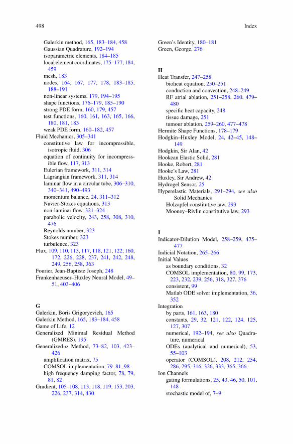
498 Index

Galerkin method, 165, 183–184, 458Gaussian Quadrature, 192–194isoparametric elements, 184–185local element coordinates, 175–177, 184,459

mesh, 183nodes, 164, 167, 177, 178, 183–185,188–191

non-linear systems, 179, 194–195shape functions, 176–179, 185–190strong PDE form, 160, 179, 457test functions, 160, 161, 163, 165, 166,180, 181, 183

weak PDE form, 160–182, 457Fluid Mechanics, 305–341

constitutive law for incompressible,isotropic fluid, 306

equation of continuity for incompress-ible flow, 117, 313

Eulerian framework, 311, 314Lagrangian framework, 311, 314laminar flow in a circular tube, 306–310,340–341, 490–493

momentum balance, 24, 311–312Navier-Stokes equations, 313non-laminar flow, 321–324parabolic velocity, 243, 258, 308, 310,476

Reynolds number, 323Stokes number, 323turbulence, 323

Flux, 109, 110, 113, 117, 118, 121, 122, 160,172, 226, 228, 237, 241, 242, 248,249, 256, 258, 363

Fourier, Jean-Baptiste Joseph, 248Frankenhaeuser–Huxley Neural Model, 49–

51, 403–406

GGalerkin, Boris Grigoryevich, 165Galerkin Method, 165, 183–184, 458Game of Life, 12Generalized Minimal Residual Method

(GMRES), 195Generalized-α Method, 73–82, 103, 423–

426amplification matrix, 75COMSOL implementation, 79–81, 98high frequency damping factor, 78, 79,81, 82

Gradient, 105–108, 113, 118, 119, 153, 203,226, 237, 314, 430

Green’s Identity, 180–181Green, George, 276

HHeat Transfer, 247–258

bioheat equation, 250–251conduction and convection, 248–249RF atrial ablation, 251–258, 260, 479–480

specific heat capacity, 248tissue damage, 251tumour ablation, 259–260, 477–478

Hermite Shape Functions, 178–179Hodgkin–Huxley Model, 24, 42–45, 148–

149Hodgkin, Sir Alan, 42Hookean Elastic Solid, 281Hooke, Robert, 281Hooke’s Law, 281Huxley, Sir Andrew, 42Hydrogel Sensor, 25Hyperelastic Materials, 291–294, see also

Solid MechanicsHolzapfel constitutive law, 293Mooney–Rivlin constitutive law, 293

IIndicator-Dilution Model, 258–259, 475–

477Indicial Notation, 265–266Initial Values

as boundary conditions, 32COMSOL implementation, 80, 99, 173,223, 232, 239, 256, 318, 327, 376

consistent, 99Matlab ODE solver implementation, 36,352

Integrationby parts, 161, 163, 180constants, 29, 32, 121, 122, 124, 125,127, 307

numerical, 192–194, see also Quadra-ture, numerical

ODEs (analytical and numerical), 53,55–103

operator (COMSOL), 208, 212, 254,286, 295, 316, 326, 333, 365, 366

Ion Channelsgating formulations, 25, 43, 46, 50, 101,148

stochastic model of, 7–9

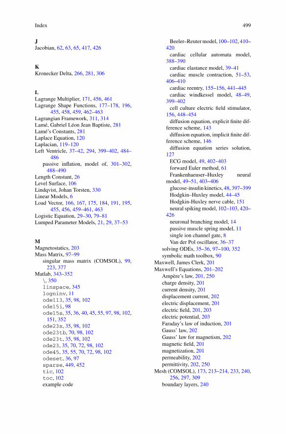
Index 499

JJacobian, 62, 63, 65, 417, 426

KKronecker Delta, 266, 281, 306

LLagrange Multiplier, 171, 456, 461Lagrange Shape Functions, 177–178, 196,

455, 458, 459, 462–463Lagrangian Framework, 311, 314Lamé, Gabriel Léon Jean Baptiste, 281Lamé’s Constants, 281Laplace Equation, 120Laplacian, 119–120Left Ventricle, 37–42, 294, 399–402, 484–

486passive inflation, model of, 301–302,488–490

Length Constant, 26Level Surface, 106Lindqvist, Johan Torsten, 330Linear Models, 6Load Vector, 166, 167, 175, 184, 191, 195,

455, 456, 459–461, 463Logistic Equation, 29–30, 79–81Lumped Parameter Models, 21, 29, 37–53

MMagnetostatics, 203Mass Matrix, 97–99

singular mass matrix (COMSOL), 99,223, 377

Matlab, 343–352\, 350linspace, 345logninv, 11ode113, 35, 98, 102ode15i, 98ode15s, 35, 36, 40, 45, 55, 97, 98, 102,151, 352

ode23s, 35, 98, 102ode23tb, 70, 98, 102ode23t, 35, 98, 102ode23, 35, 70, 72, 98, 102ode45, 35, 55, 70, 72, 98, 102odeset, 36, 97sparse, 449, 452tic, 102toc, 102example code

Beeler–Reutermodel, 100–102, 410–420cardiac cellular automata model,

388–390cardiac elastance model, 39–41cardiac muscle contraction, 51–53,

406–410cardiac reentry, 155–156, 441–445cardiac windkessel model, 48–49,

399–402cell culture electric field stimulator,

156, 448–454diffusion equation, explicit finite dif-

ference scheme, 143diffusion equation, implicit finite dif-

ference scheme, 146diffusion equation series solution,

127ECG model, 49, 402–403forward Euler method, 61Frankenhaeuser–Huxley neural

model, 49–51, 403–406glucose-insulin kinetics, 48, 397–399Hodgkin–Huxley model, 44–45Hodgkin-Huxley nerve cable, 151neural spiking model, 102–103, 420–

426neuronal branching model, 14passive muscle spring model, 11single ion channel gate, 8Van der Pol oscillator, 36–37

solving ODEs, 35–36, 97–100, 352symbolic math toolbox, 90

Maxwell, James Clerk, 201Maxwell’s Equations, 201–202

Ampère’s law, 201, 250charge density, 201current density, 201displacement current, 202electric displacement, 201electric field, 201, 203electric potential, 203Faraday’s law of induction, 201Gauss’ law, 202Gauss’ law for magnetism, 202magnetic field, 201magnetization, 201permeability, 202permittivity, 202, 250

Mesh (COMSOL), 173, 213–214, 233, 240,256, 297, 309

boundary layers, 240

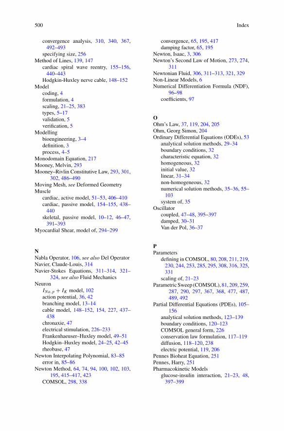
500 Index

convergence analysis, 310, 340, 367,492–493

specifying size, 256Method of Lines, 139, 147

cardiac spiral wave reentry, 155–156,440–443

Hodgkin-Huxley nerve cable, 148–152Model

coding, 4formulation, 4scaling, 21–25, 383types, 5–17validation, 5verification, 5

Modellingbioengineering, 3–4definition, 3process, 4–5

Monodomain Equation, 217Mooney, Melvin, 293Mooney–Rivlin Constitutive Law, 293, 301,

302, 486–490Moving Mesh, see Deformed GeometryMuscle

cardiac, active model, 51–53, 406–410cardiac, passive model, 154–155, 438–440

skeletal, passive model, 10–12, 46–47,391–393

Myocardial Shear, model of, 294–299

NNabla Operator, 106, see also Del OperatorNavier, Claude-Louis, 314Navier-Stokes Equations, 311–314, 321–

324, see also Fluid MechanicsNeuron

INa,p + IK model, 102action potential, 36, 42branching model, 13–14cable model, 148–152, 154, 227, 437–438

chronaxie, 47electrical stimulation, 226–233Frankenhaeuser–Huxley model, 49–51Hodgkin–Huxley model, 24–25, 42–45rheobase, 47

Newton Interpolating Polynomial, 83–85error in, 85–86

Newton Method, 64, 74, 94, 100, 102, 103,195, 415–417, 423

COMSOL, 298, 338

convergence, 65, 195, 417damping factor, 65, 195

Newton, Isaac, 3, 306Newton’s Second Law of Motion, 273, 274,

311Newtonian Fluid, 306, 311–313, 321, 329Non-Linear Models, 6Numerical Differentiation Formula (NDF),

96–98coefficients, 97

OOhm’s Law, 37, 119, 204, 205Ohm, Georg Simon, 204Ordinary Differential Equations (ODEs), 53

analytical solution methods, 29–34boundary conditions, 32characteristic equation, 32homogeneous, 32initial value, 32linear, 31–34non-homogeneous, 32numerical solution methods, 35–36, 55–103

system of, 35Oscillator

coupled, 47–48, 395–397damped, 30–31Van der Pol, 36–37

PParameters

defining in COMSOL, 80, 208, 211, 219,230, 244, 253, 285, 295, 308, 316, 325,331

scaling of, 21–23Parametric Sweep (COMSOL), 81, 209, 259,

287, 290, 297, 367, 368, 477, 487,489, 492

Partial Differential Equations (PDEs), 105–156

analytical solution methods, 123–139boundary conditions, 120–123COMSOL general form, 226conservation law formulation, 117–119diffusion, 118–120, 238electric potential, 119, 206

Pennes Bioheat Equation, 251Pennes, Harry, 251Pharmacokinetic Models

glucose-insulin interaction, 21–23, 48,397–399

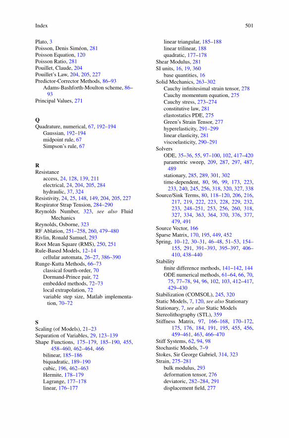
Index 501

Plato, 3Poisson, Denis Siméon, 281Poisson Equation, 120Poisson Ratio, 281Pouillet, Claude, 204Pouillet’s Law, 204, 205, 227Predictor-Corrector Methods, 86–93

Adams-Bashforth-Moulton scheme, 86–93

Principal Values, 271

QQuadrature, numerical, 67, 192–194

Gaussian, 192–194midpoint rule, 67Simpson’s rule, 67

RResistance

access, 24, 128, 139, 211electrical, 24, 204, 205, 284hydraulic, 37, 324

Resistivity, 24, 25, 148, 149, 204, 205, 227Respirator Strap Tension, 284–290Reynolds Number, 323, see also Fluid

MechanicsReynolds, Osborne, 323RF Ablation, 251–258, 260, 479–480Rivlin, Ronald Samuel, 293Root Mean Square (RMS), 250, 251Rule-Based Models, 12–14

cellular automata, 26–27, 386–390Runge-Kutta Methods, 66–73

classical fourth-order, 70Dormand-Prince pair, 72embedded methods, 72–73local extrapolation, 72variable step size, Matlab implementa-tion, 70–72

SScaling (of Models), 21–23Separation of Variables, 29, 123–139Shape Functions, 175–179, 185–190, 455,

458–460, 462–464, 466bilinear, 185–186biquadratic, 189–190cubic, 196, 462–463Hermite, 178–179Lagrange, 177–178linear, 176–177

linear triangular, 185–188linear trilinear, 188quadratic, 177–178

Shear Modulus, 281SI units, 16, 19, 360

base quantities, 16Solid Mechanics, 263–302

Cauchy infinitesimal strain tensor, 278Cauchy momentum equation, 275Cauchy stress, 273–274constitutive law, 281elastostatics PDE, 275Green’s Strain Tensor, 277hyperelasticity, 291–299linear elasticity, 281viscoelasticity, 290–291

SolversODE, 35–36, 55, 97–100, 102, 417–420parametric sweep, 209, 287, 297, 487,489

stationary, 285, 289, 301, 302time-dependent, 80, 96, 99, 173, 223,233, 240, 245, 256, 318, 320, 327, 338

Source/Sink Terms, 80, 118–120, 206, 216,217, 219, 222, 223, 228, 229, 232,233, 248–251, 253, 256, 260, 318,327, 334, 363, 364, 370, 376, 377,479, 491

Source Vector, 166Sparse Matrix, 170, 195, 449, 452Spring, 10–12, 30–31, 46–48, 51–53, 154–

155, 291, 391–393, 395–397, 406–410, 438–440

Stabilityfinite difference methods, 141–142, 144ODE numerical methods, 61–64, 66, 70,75, 77–78, 94, 96, 102, 103, 412–417,429–430

Stabilization (COMSOL), 245, 320Static Models, 7, 120, see also StationaryStationary, 7, see also Static ModelsStereolithography (STL), 359Stiffness Matrix, 97, 166–168, 170–172,

175, 176, 184, 191, 195, 455, 456,459–461, 463, 466–470

Stiff Systems, 62, 94, 98Stochastic Models, 7–9Stokes, Sir George Gabriel, 314, 323Strain, 275–281

bulk modulus, 293deformation tensor, 276deviatoric, 282–284, 291displacement field, 277

502 Index

hydrostatic, 282–284invariants, 292isochoric right Cauchy–Green deforma-tion tensor, 293

left Cauchy–Green deformation tensor,276

principal stretch ratios, 292–293pure extension, 280right Cauchy–Green deformation tensor,276

shear, 280–281, 294–299strain energy, 283, 291–294volumetric strain, 278

Strain Gauge, modelling of, 284–290Strain Rate, 305–306, 312

shear rate, 329Stress, 271–275

Cauchy stress, 273deviatoric, 282–284, 291hydrostatic, 282–284shear, 18state of stress, 273symmetric tensor, 273traction (or stress vector), 271–272viscous, 306, 307von Mises, 283, 284, 288, 289von Mises Stress, 298

Symmetric Matrix, 170, 171Systems Biology, 3, 343

TTaylor’s Theorem, 55–59

multivariate form, 58–59univariate form, 55

Tensors, 263–265conductivity tensor, 205, 218dyadic components, 264invariants, 268–271principal axes, 271principal values, 271strain tensor, 277, 278stress tensor, 272symmetric, 205transformation law, 266–268

Tetrodotoxin (TTX), 51Time-Dependent, 7, see alsoDynamicMod-

elsTorque, 333–335Trapezoidal Method, 65–66

UUnits

dimensional analysis, 16–19, 23–24,382–383

use in COMSOL, 80, 81, 219, 224, 229,233, 253, 257, 287, 288, 290, 299, 318,327, 328, 334, 360–361, 364, 370, 378,379

VValidation of Models, 4, 5Variables, 7, 10, 21, 29, 30

COMSOL units of, 219, 229, 333, 334,370

global (Matlab), 40state, 35, 36, 38, 39, 41

Vectorcross product, 112, 114dot product, 106field, 106, 108

Verification of Models, 4, 5Virtual Reality Modelling Language

(VRML), 359Viscoelasticity, 290–291, see also Solid

MechanicsViscosity, 18–21, 24, 306, 313, 329–330Volume Conductor, 204–207Von Mises, Richard Edler, 283

WWindkessel Models, 48, 399–402

YYoung’s Modulus, 281Young, Thomas, 281

Matlab Fundamentals

Documents