Matlab Basics

Matlab Basics

Juha KuorttiOctober 21, 2017

1

First steps

Meet the IDEGetting HelpBasic scalar variables.

2

1. What, where, how

• Matrix laboratory [Cleve Moler, Mathworks inc.]• Language and tool for numerical computation• Large number of mathematical and other functions.• Functional programming language, user can extend Matlab by

defining (programming) own functions.• Application specific toolboxes• http://se.mathworks.com/help/matlab/index.html• http://www.mathworks.se/academia/• http://se.mathworks.com/help/matlab/examples/basic-

matrix-operations.html?prodcode=ML• google: learn matlab, matlab <keyword>

3

help,doc,lookfor

• help, doc• >> doc starts help system, same as ?• >> help name >> doc name

help is faster, doc is more comprehensive.• Some search words for help/doc:

elfun – elementary functionsgeneral, ops, elmat, ... More on next slide

• lookfor>> lookfor sum, lookfor solve

>> lookfor optimize, lookfor equation

Beware: Some searches may give too many hits.• google Matlab,<keywords, phrases>

4

Some help-keywords »help

general - General purpose commandsops - Operators and spec. charslang - Programming language constructselmat - Elementary matriceselfun - Elementary functionsspecfun - Special functuonsmatfun - Matrix functionsdatafun - Data analysis and Fourier transformgraph2d - 2d graphicsgraph3d - 3d graphicsgraphics - Handle graphicsimagesci - Image and scientific datademos - Examples and demo’s

Comprehensive set of keywords 5

First steps and concepts

• Workspace, commandwindow

• Matrices and otherdatatypes are stored inmemory, contents areshown in workspace..

• » who, whos

• Commands (functions) areapplied to variables in theworkspace.

• Matlab interprets andreturns the result(s) inthe workspace. (Ordisplays an errormessage)

1. Start Matlab2. Create a working

directory: EitherFile-menu or command>> mkdir mydir a)

3. >> cd mydir

4. Create variable:>> x=5

5. Do: >> y=exp(x)

6. Try >> who, whos

aSome Unix/Linux-commands can be givenin the Matlab command window

6

First steps and concepts

• Workspace, commandwindow

• Matrices and otherdatatypes are stored inmemory, contents areshown in workspace..

• » who, whos

• Commands (functions) areapplied to variables in theworkspace.

• Matlab interprets andreturns the result(s) inthe workspace. (Ordisplays an errormessage)

1. Start Matlab2. Create a working

directory: EitherFile-menu or command>> mkdir mydir a)

3. >> cd mydir

4. Create variable:>> x=5

5. Do: >> y=exp(x)

6. Try >> who, whos

aSome Unix/Linux-commands can be givenin the Matlab command window

6

Working in the command window

• “Undoc” command window (or make it large enough)• Here’s a possible first session, try yourself!

>> 3/4

ans =

0.7500

>> 4*ans

ans =

3

>> r=3/4; % Supress output

>> r % Show result

r =

0.7500

>> Area=pi*r^2

Area =

1.76717

Arithmetic operations, examples

• Multiplication and division from left to right, equalprecedence.

• Ordinary precedence rules. Use parentheses for clearity !

>> 6/3*2 >> 6/3/2

ans = 4 ans = 1

>> 6/(3*2) >> 6/(3/2)

ans = 1 ans = 4

8

Exercise

Make the following variables:

• a = 10• b = 2.51023

• c = 2 + 3i (i being the imaginary unit)• d =e 2

3πi

9

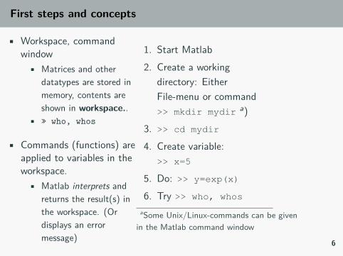
Arithmetic, precedence

Scalar arithmetic operations

Symbol Name Math Matlab+,- add/subtract a ± b a+b,a-b* multiply ab a*b/ Righ divide a

b a/b 1

\ Left divide ba a\b 2

^ power ab a^b

1Recommendation:Use this for scalar division2Recommendation:Use this for “matrix division”

10

Command window, history, create script

Command window:

• Use the up-arrow key to scroll back through the commands.• Use the down-arrow key to scroll forward• Edit a line using the left- and right-arrow keys.• Press the Enter key to execute the command

Create script from command history:

• Choose commands from the history with CTR + mouse left .Mouse right lets you choose “create script”. (More on scriptssoon.)

• Execute commands from the editor: CTR-Enter .

11

Little scalar task, work together

• The volume of a circular cylinder of height h and radius r isgiven by V = πr2h. A particular cylindrical tank is 15 m highand has a radius of 8 m. We want to construct anothercylindrical tank with a volume 20 percent greater but havingthe same height. How large must its radius be?

12

Solution, command history, make script

Here’s the Matlab-session:

>>r = 8;

>>h = 15;

>>V = pi*r^2*h;

>>V = 1.2*V; % 20% increase in V

>>r = sqrt(V/(pi*h))

r =

8.7636

Use ↑ for command history. With CTR+Mouse left paintcommands you want to save, press mouse right and choose “makescript”.

13

Scripts, publish

You can perform operations in MATLAB in two ways:

• In the interactive mode, in which all commands are entereddirectly in the Command window.

• By running a MATLAB program stored in a script file. Thistype of file contains MATLAB commands, so running it isequivalent to typing all the commands—one at a time—at theCommand window prompt. You can run the file by typing itsname at the Command window prompt.

• The script file commands can also be executed directly fromMatlab’s editor window either by parts or all of them.

• publish produces a well structured document of running thescript.

14

Examples of expressions

>> 6*sqrt(2)+pi^2

ans=18.3549

>> one=sin(pi/3)^2 + cos(pi/3)^2

one = 1

>> 1==sin(pi/3)^2 + cos(pi/3)^2 % Equal?

ans = 1 % Logical: true

>> exp(i*pi) % Not e^x !!

>> 1.0/0.0 -> Inf

>> -4/Inf -> 0

>> 0/0 -> NaN % "Not-a-number".

>> format long % Show max number of digits.

>> [1+eps,1+3*eps] % eps: Limit of rel. accuracy.

>> format short % Back to default display.

>> clc % Clean display.

>> clear % Remove all variables from ws.

15

Workspace

• Variables are stored in the memory and accessed in theworkspace

• Commands for managing the workspace are called here“system commands”, perhaps a little “unofficially”. Forinstance who, whos show variables in the workspace, latterwith sizes.

• clear erases all variables from the workspace (memory), clearvar1 var2 erases these variables.

• The syntax of “system commands” differs from computationaland other functions. System commands don’t useparenteheses or commas.

16

Some “system commands”

Some commands for managing the workspace

Matlab command Descriptionclc Clear command window (visually).clear Clear all variables (from memory).clear var1 var2 Clear these variables.who List variables in memorywhos List variables with sizes in memoryformat Display format of numbersclf Clear current graphics window.close all Close all graphics windows.shg Show Graphics.

17

Comparison, relations, scalar case

• Remember: name = expression means assignment of thevalue of expression to variable name.

• lhs == rhs Returns 1 if equal,0 if not.• <, <=, >, >=, ∼= are other arithmetic comparisons.• The value of a comparison is true (1) or false (0).• Precedence of arithmetics is higher than that of comparisons

>> 1==0 % --> ans = 0

>> E = 1.733>tan(pi/3) % --> E = 1

What are the results ? : >> E=4>5-2 , (4>5)-2

18

Expression, variable, special variable ans

• An expression consists of numbers, variables, functions,operators such as+,-,*,/,^,(), sin, cos, exp, abs, ...

• help/doc ops,elfun [See previous slide for more searchwords.]• >> var=expression

assigns the value of expression to variable var.• If the expression is written without an assignment, the result

is assigned to the special variable ans.Note: ans holds just the previous result, the next suchcomputation overwrites it.

19

Variable names and types

Variable names:

• Start with a letter, then letters, numbers, underscore( _)• Other special characters not allowed, especially minus (-) is

not possible, as it means subtraction.• CASE SENSITIVE! ( var1 is different from Var1)

NOTE: Matlab help texts: old style (from 1980’s) of capitalizedNAME meaning name, Let’s abandon this usage.

>> number=-2.345

>> % Note: period (.), not comma (,)

>> complex_number=3+4*i

>> n=1;n=n+1;

>> string=['This is trial nr. ' num2str(n)]

>> length(string)

ans = 19 20

Variable names and types

• No need to initialize or define a variable, if efficiency is not anissue (return to this later).

• Default type is 64 bits floating point number ("double"),about 16 decimal digits.

>> 2.345• Characters are of type ’char’ (16 bits)

>> ’this is a character string’• Change numeric data into character

>> num2str(2.3)>> str2num(ans) % and back

• Other tyes: logical, single,int-typeshelp datatypeshttps://se.mathworks.com/help/matlab/numeric-types.html

21

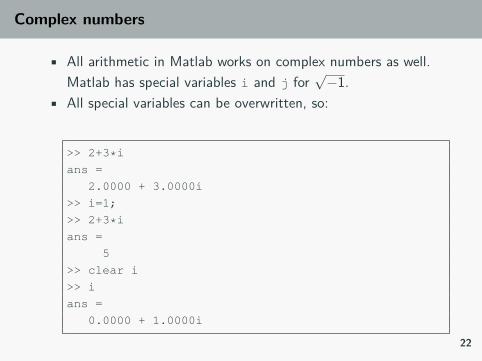
Complex numbers

• All arithmetic in Matlab works on complex numbers as well.Matlab has special variables i and j for

√−1.

• All special variables can be overwritten, so:

>> 2+3*i

ans =

2.0000 + 3.0000i

>> i=1;

>> 2+3*i

ans =

5

>> clear i

>> i

ans =

0.0000 + 1.0000i

22

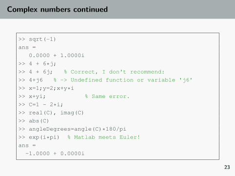
Complex numbers continued

>> sqrt(-1)

ans =

0.0000 + 1.0000i

>> 4 + 6*j;

>> 4 + 6j; % Correct, I don't recommend:

>> 4+j6 % -> Undefined function or variable 'j6'

>> x=1;y=2;x+y*i

>> x+yi; % Same error.

>> C=1 - 2*i;

>> real(C), imag(C)

>> abs(C)

>> angleDegrees=angle(C)*180/pi

>> exp(i*pi) % Matlab meets Euler!

ans =

-1.0000 + 0.0000i

23

Dimensional increase

VectorsMatricesArrays.

24

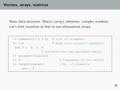
Vectors, arrays, matrices

Basic data structure: Matrix (array), elements: complex numbers.Let’s limit ourselves at first to two-dimensional arrays.

>> rowvect=[1 2 3 4] % List of elements

>> 1:4 % Same with colon(:)-operator

ans = 1 2 3 4

% ans:previous non-assigned result

>> colvect=[1;2;3;4]

>> v' % Transpose of row-vector

>> length(rowvect) % Nr. of elements

ans = 4

25

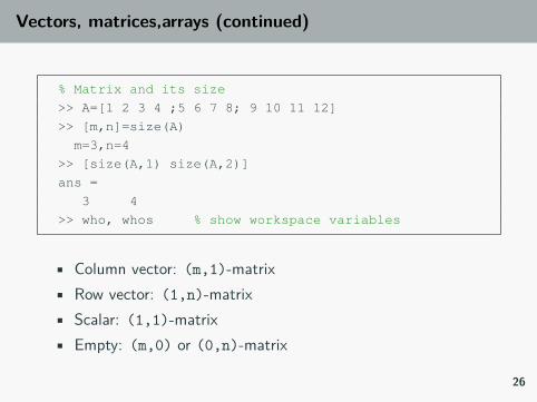
Vectors, matrices,arrays (continued)

% Matrix and its size

>> A=[1 2 3 4 ;5 6 7 8; 9 10 11 12]

>> [m,n]=size(A)

m=3,n=4

>> [size(A,1) size(A,2)]

ans =

3 4

>> who, whos % show workspace variables

• Column vector: (m,1)-matrix• Row vector: (1,n)-matrix• Scalar: (1,1)-matrix• Empty: (m,0) or (0,n)-matrix

26

Calculus with vectors

• The numbers 0, 0.1, 0.2, . . . , 10 can be assigned to thevariable u by typing u = 0:0.1:10;

• length(u) reveals us that there are 101 elements in u.• To compute w = 5 sin u for u = 0, 0.1, 0.2, . . . , 10, the session

is;

>>u = 0:0.1:10; % By 'misuse' of Matlab:

>>w = 5*sin(u); >>for k=1:length(u)

w(k)=5*sin(u(k));

end;toc

• This was our first acquaintance with “vectorization”.

27

Vector excercise

Make the following variables:

• aVec =[3.14 15 9 26]

]

• bVec =

2.71828182

• cVec= [5, 4.8, . . . ,−4.8,−5] (all the numbers from 5 to -5

with increments of -0.2)• dVec = [100 100.01 . . . 100.99 101] logarithmically spaced

numbers between 1 and 10.• eVec = ’Hello there’ (eVec is a string, which is a vector of

characters)

28

“Scalar functions” support vectorization

The previous example leads us to the following general idea:Functions which applied to a scalar produce a scalar result arecalled scalar functions (perhaps a bit misleadingly). When suchfunctions are applied to a vector, they operate on every element ofthe vector. Mathematical functions help elfun, specfun

among others are of this type.

>> t = [-1 0 1];

>> y = exp(t)

y =

0.3679 1.0000 2.7183

>> [exp(-1) exp(0) exp(1)]

ans =

0.3679 1.0000 2.7183

29

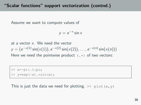
“Scalar functions” support vectorization (contnd.)

Assume we want to compute values of

y = e−x sin x

at a vector x . We need the vectory = (e−x(1) sin(x(1)), e−x(2) sin(x(2)), . . . , e−x(n) sin(x(n)))Here we need the pointwise product (.*) of two vectors:

>> x=-pi:.1:pi;

>> y=exp(-x).*sin(x);

This is just the data we need for plotting. >> plot(x,y)

30

Functions for building vectorscolon(:),linspace,logspace

• v=a:b, w=a:h:b; default: h=1• v=linspace(a,b,N); default: N=100• v=logspace(a,b,N); 10a, . . . , 10b, N points

>> 0:10; 0:.1:1;

>> 10:-2:0

ans =

10 8 6 4 2 0

>> logspace(0,1,4)

ans =

1.0000 2.1544 4.6416 10.0000

>> 10.^linspace(0,1,4)

ans =

1.0000 2.1544 4.6416 10.0000

Note: Remember semicolon (;) for large N or small h. 31

Matrices: building, parts, decomposing

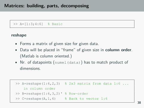
>> A=[1:3;4:6] % Basic

reshape

• Forms a matrix of given size for given data.• Data will be placed in “frame” of given size in column order.

(Matlab is column oriented.)• Nr. of datapoints (numel(data)) has to match product of

dimensions.

>> A=reshape(1:6,2,3) % 2x3 matrix from data 1:6 ...

in column order

>> B=reshape(1:6,3,2)' % Row-order

>> C=reshape(A,1,6) % Back to vector 1:632

Array, matrix,vector,scalar

• Basic data structurte: Matrix (array), elements: complexnumbers. Let’s limit ourselves at first to two-dimensionalarrays.

• Column vector: (m,1)-matrix• Row vector: (1,n)-matrix• Scalar: (1,1)-matrix• Empty: (m,0) or (0,n)-matrix

• Matrix and its (size)

>> A=[1 2 3 4 ;5 6 7 8; 9 10 11 12]

>> [m,n]=size(A)

>> v=-[1 2 3 4 ]

>> length(v)

>> 1:10 % [1,2,3,...,10]

>> size(ans) % ans:previous non-assigned result

>> who, whos % workspace variables33

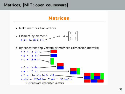
Matrices, [MIT: open courseware]

34

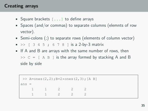
Creating arrays

• Square brackets [...] to define arrays• Spaces (and/or commas) to separate columns (elemnts of row

vector).• Semi-colons (;) to separate rows (elements of column vector)• >> [ 3 4 5 ; 6 7 8 ] is a 2-by-3 matrix• If A and B are arrays with the same number of rows, then

>> C = [ A B ] is the array formed by stacking A and Bside by side

>> A=ones(2,2);B=2*ones(2,3);[A B]

ans =

1 1 2 2 2

1 1 2 2 2

35

Creating arrays, continued

• If A and B are arrays with the same number of columns, then>> [ A ; B ] is the array formed by stacking A on top of B.

• So, [[ 3 ; 6 ] [ 4 5 ; 7 8 ] ] is equal to[ 3 4 5;6 7 8 ]

36

Some functions for building matrices

eye,vander,hilb,zeros,ones,diag,rand,reshape,magic

Complete list: help elmat

>> A = zeros(2,5)

>> B = ones(3) % or ones(3,3)

>> R = rand(3,2)

>> N = randn(3,2)

>> D = diag(-2:2)

Compare rand and randn Try repeatedly>> R = rand(3,2) Use (↑) in command window

Repeat : >>rand('twister',0); R = rand(3,2)

37

Matrices: building, parts, decomposing

>> A=[1:3;4:6] % Basic

reshape

• Forms a matrix of given size for given data.• Data will be placed in “frame” of given size in column order.

(Matlab is column oriented.)• Nr. of datapoints (numel(data)) has to match product of

dimensions.

>> A=reshape(1:6,2,3) % 2x3 matrix from data 1:6 ...

in column order

>> B=reshape(1:6,3,2)' % Row-order

>> C=reshape(A,1,6) % Back to vector 1:638

Matrices, building blocks

>> A=reshape(1:6,2,3); B=ones(2,2),C=diag(1:3)

>> [A B] % Side by side.

ans =

1 3 5 1 1

2 4 6 1 1

>> [A;C] % On top of each other.

ans =

1 3 5

2 4 6

1 0 0

0 2 0

0 0 3

39

Matrix- and array algebra

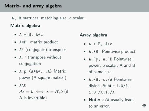
A, B matrices, matching size, c scalar.Matrix algebra

• A + B, A+c

• A*B matrix product• A’ (conjugate) transpose• A.’ transpose without

conjugation• A^p (A*A*...A) Matrix

power (A square matrix.)• A\b

Ax = b ⇐⇒ x = A\b (ifA is invertible)

Array algebra

• A + B, A+c

• A.*B Pointwise product• A.^p, A.^B Pointwise

power, p scalar, A and Bof same size.

• A./B, c./A Pointwisedivide. Subtle 1.0/A,1.0./A,1./A

• Note: c/A usually leadsto an error. 40

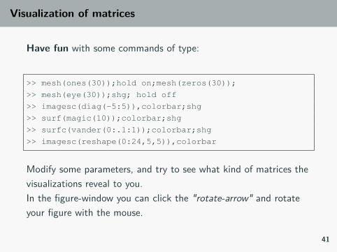
Visualization of matrices

Have fun with some commands of type:

>> mesh(ones(30));hold on;mesh(zeros(30));

>> mesh(eye(30));shg; hold off

>> imagesc(diag(-5:5)),colorbar;shg

>> surf(magic(10));colorbar;shg

>> surfc(vander(0:.1:1));colorbar;shg

>> imagesc(reshape(0:24,5,5)),colorbar

Modify some parameters, and try to see what kind of matrices thevisualizations reveal to you.In the figure-window you can click the "rotate-arrow" and rotateyour figure with the mouse.

41

Accessing single element of a vector

If A is a vector, then• A(1) is its first element• A(2) is its second element• . . .

• A(end) is its last element

For matrices either columnwise linear indexing,or

• A(1,1) is the element on the first row ofthe first column

• A(2,1) is the element on the second rowof the first column

• A(3,4) is the element on the third row andfourth column

• A(4,end) is the last element of the fourthrow

42

Example

>> A = [ 3 4.2 -7 10.1 0.4 -3.5 ];

>> A(3)

>> Index = 5;

>> A(Index)

>> A(4) = log(8);

>> A

>> A(end)

43

Accessing multiple elements of an array

Index need not be a single number – you can index with a vector.

>> A = [ 3 4.2 -7 10.1 0.4 -3.5 ];

>> A([1 4 6]) % 1-by-3, 1st, 4th, 6th entry

>> Index = [3 2 3 5];

>> A(Index) % 1-by-4

Index should contain integers. Shape of the index will define theshape of the output array.

44

Exercise

Using MATLAB indexing, compute the perimeter sum of thematrix “magic(8)”.

Perimeter sum adds together the elements that are in the first andlast rows and columns of the matrix. Try to make your codeindependent of the matrix dimensions using end.

45

46

Linear Systems

47

Linear systems of equations

Given the system of equations:6x + 12y + 4z = 707x − 2y + 3z = 52x + 8y − 9z = 64

Solve it!

>> A=[6 12 4;7 -2 3;2 8 -9]

>> b=[70;5;64];

>> x=A\b; x'

ans =

3 5 -2

48

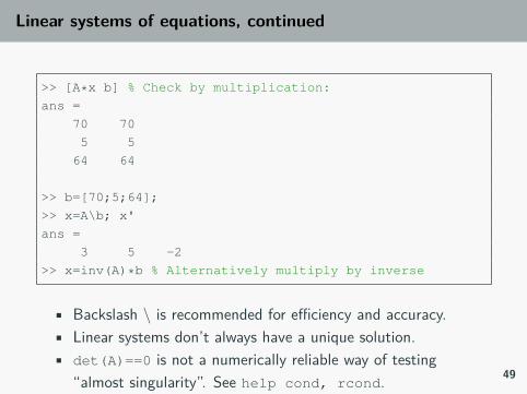
Linear systems of equations, continued

>> [A*x b] % Check by multiplication:

ans =

70 70

5 5

64 64

>> b=[70;5;64];

>> x=A\b; x'

ans =

3 5 -2

>> x=inv(A)*b % Alternatively multiply by inverse

• Backslash \ is recommended for efficiency and accuracy.• Linear systems don’t always have a unique solution.• det(A)==0 is not a numerically reliable way of testing

“almost singularity”. See help cond, rcond. 49

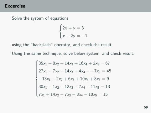
Excercise

Solve the system of equations2x + y = 3x − 2y = −1

using the “backslash” operator, and check the result.

Using the same technique, solve below system, and check result.

35x1 + 0x2 + 14x3 + 16x4 + 2x5 = 6727x1 + 7x2 + 14x3 + 4x4 +−7x5 = 45−13x1 − 2x2 + 6x3 + 10x4 + 8x5 = 930x1 − 1x2 − 12x3 + 7x4 − 11x5 = 137x1 + 14x2 + 7x3 − 3x4 − 10x5 = 15

50

Functions

51

User-defined functions

• Function handles, anonymous functions• One-liners, defined in the command window or in a script

>> f=@(x)x.^2 to be read: f is the function which“at x” returns the value x2. (In math: f = x → x2)Several inputs allowed:>> g=@(x,y,z)sqrt(x.^2+y.^2+z.^2).

• Functions in m-filesIf more lines are needed, local variables, control structures(for, while, if - else, etc.), then write an m-file

• Inline-function is older, more restrictive version of functionhandle. We will not use them actively, the only reason toknow about them, is old Matlab-codes. (help inline)

52

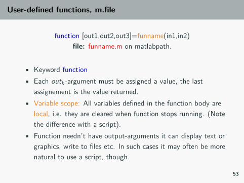
User-defined functions, m.file

function [out1,out2,out3]=funname(in1,in2)file: funname.m on matlabpath.

• Keyword function• Each outk -argument must be assigned a value, the last

assignement is the value returned.• Variable scope: All variables defined in the function body are

local, i.e. they are cleared when function stops running. (Notethe difference with a script).

• Function needn’t have output-arguments it can display text orgraphics, write to files etc. In such cases it may often be morenatural to use a script, though.

53

Examples of writing functions

To start editing a function, open theeditor on the top left “New”-button.Instead of script, this time clickFunction. Or on the command line:>> edit myfunction

As our first example, let’s write a function that computes the meanof the components of the input vector.Let’s first give some thought of the expression.

x=1:10;

avg=sum(x)/length(x)

54

Examples of writing functions

To start editing a function, open theeditor on the top left “New”-button.Instead of script, this time clickFunction. Or on the command line:>> edit myfunction

As our first example, let’s write a function that computes the meanof the components of the input vector.Let’s first give some thought of the expression.

x=1:10;

avg=sum(x)/length(x)

54

Example 1, mean of a vector

function y=mymean(x)

% Compute the mean (average) ox x-values.

% Input: vector x

% Result : mean of x

% Exampe call: r=mymean(1:10)

%

y=sum(x)/length(x);

>> help mymean

Compute the mean (average) ox x-values.

...

>> r=mymean(1:10)

r =

5.5000

55

Example 2.: function stats

Standard deviation is given by:

σ =

√√√√ 1N

n∑k=1

(xk − µ)2.

Write the code for the following function file:

function [avg,sd,range] = stats(x)

% Returns the average (mean), standard deviation

% and range of input vector x

N=length(x);

...

...

56

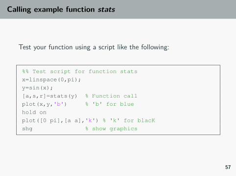
Calling example function stats

Test your function using a script like the following:

%% Test script for function stats

x=linspace(0,pi);

y=sin(x);

[a,s,r]=stats(y) % Function call

plot(x,y,'b') % 'b' for blue

hold on

plot([0 pi],[a a],'k') % 'k' for blacK

shg % show graphics

57

Solution: Listing of function stats

function [avg,sd,range] = stats(x)

% Returns the average (mean), standard deviation

% and range of input vector x

N=length(x);

avg=sum(x)/N;

sd = sqrt(sum(x - avg).^2)/N);

range=[min(x),max(x)];

58

Basics of Graphics

59

Basic 2d-graphics, plot

• "Matlab has excellent support for data visualization andgraphics with over 70 types of plots currently available. Wewon’t be able to go into all of them here, nor will we need to,as they all operate in very similar ways. In fact, byunderstanding how Matlab plotting works in general, we’ll beable to see most plot types as simple variations of each other.Fundamentally, they all use the same basic constructs."

• Links:- https://se.mathworks.com/help/matlab/ref/plot.html- http://ubcmatlabguide.github.io/html/plotting.html

60

Basic 2d-graphics

• If x is a 1-by-N (or N-by-1) vector, and y is a 1-by-N (orN-by-1) vector, then>> plot(x,y)

creates a figure window, and plots the data points with joiningline segments in the axes. The points are:(x(1),y(1)), (x(2),y(2)),..., (x(N),y(N))

• The axes are automatically chosen so that all data just fitsinto the figure window. This can be changed by theaxis, xlim, ylim-commands.

61

Basic 2d-graphics, plot

Function plot can be used for simple "join-the-dots" xy-plots.

>> x=[1.5 2.2 3.1 4.6 5.7 6.3 9.4];

>> y=[2.3 3.9 4.3 7.2 4.5 6.1 1.1];

>> plot(x,y);grid on

62

Basic 2d-graphics, general form

Continue keeping the previous plot:

>> hold on % Keep the previous lines.

>> plot(x,y,'or') % Mark datapoints with ...

'o'-marker, r='red'

>> shg % show graphics

• General form:plot(x1,y1,'string1',x2,y2,'string2', ...)

The 'string'-parts may be missing.• plot(x,y,’r*--’)

Use red *-markers, join with red dashed line segments.

63

help plot -> table of markers

Various line types, plot symbols and colors: plot(X,Y,S)S is a character string made from one element from any or all ofthe following 3 columns:

b blue . point - solid

g green o circle : dotted

r red x x-mark -. dashdot

c cyan + plus -- dashed

m magenta * star (none)no line

y yellow s square

k black d diamond

w white v triangle (down)

^ triangle (up)

< triangle (left)

> triangle (right)

p,h pentagram, hexagram64

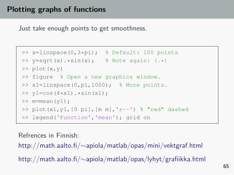
Plotting graphs of functions

Just take enough points to get smoothness.

>> x=linspace(0,3*pi); % Default: 100 points

>> y=sqrt(x).*sin(x); % Note again: (.*)

>> plot(x,y)

>> figure % Open a new graphics window.

>> x1=linspace(0,pi,1000); % More points.

>> y1=cos(4*x1).*sin(x1);

>> m=mean(y1);

>> plot(x1,y1,[0 pi],[m m],'r--') % "red" dashed

>> legend('Function','mean'); grid on

Refrences in Finnish:http://math.aalto.fi/∼apiola/matlab/opas/mini/vektgraf.html

http://math.aalto.fi/∼apiola/matlab/opas/lyhyt/grafiikka.html65

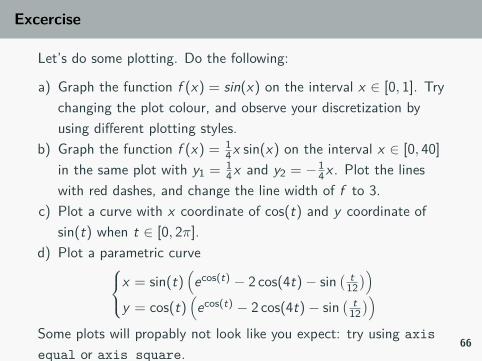
Excercise

Let’s do some plotting. Do the following:

a) Graph the function f (x) = sin(x) on the interval x ∈ [0, 1]. Trychanging the plot colour, and observe your discretization byusing different plotting styles.

b) Graph the function f (x) = 14x sin(x) on the interval x ∈ [0, 40]

in the same plot with y1 = 14x and y2 = −1

4x . Plot the lineswith red dashes, and change the line width of f to 3.

c) Plot a curve with x coordinate of cos(t) and y coordinate ofsin(t) when t ∈ [0, 2π].

d) Plot a parametric curvex = sin(t)(ecos(t) − 2 cos(4t)− sin

( t12))

y = cos(t)(ecos(t) − 2 cos(4t)− sin

( t12))

Some plots will propably not look like you expect: try using axisequal or axis square.

66

Polynomials

67

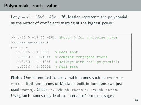
Polynomials, roots, value

Let p = x4 − 15x2 + 45x − 36. Matlab represents the polynomialas the vector of coefficients starting at the highest power:

>> c=[1 0 -15 45 -36]; %Note: 0 for a missing power

>> pzeros=roots(c)

pzeros =

-5.0355 + 0.0000 % Real root

1.8680 + 1.4184i % complex conjugate roots

1.8680 - 1.4184i % (always with real polynomial)

1.2996 + 0.0000i % Real root

Note: One is tempted to use variable names such as roots orzeros. Both are names of Matlab’s built-in functions (we justused roots). Check: >> which roots >> which zeros.Using such names may lead to “nonsense” error messages.

68

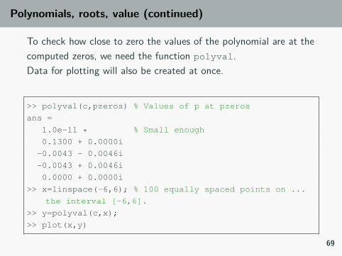
Polynomials, roots, value (continued)

To check how close to zero the values of the polynomial are at thecomputed zeros, we need the function polyval.Data for plotting will also be created at once.

>> polyval(c,pzeros) % Values of p at pzeros

ans =

1.0e-11 * % Small enough

0.1300 + 0.0000i

-0.0043 - 0.0046i

-0.0043 + 0.0046i

0.0000 + 0.0000i

>> x=linspace(-6,6); % 100 equally spaced points on ...

the interval [-6,6].

>> y=polyval(c,x);

>> plot(x,y)

69

Exercise

• Plot the values of the polynomial p(x) = x4 − 3x3 + 8x + 2on the interval x = [−3, 3].

• Find the roots of p(x).• Find the roots of z12 − 1 (Yes, there is more than one), and

plot them on the complex plane.• Construct a polynomial of degree 6, with roots rk = k. (i.e.,

first root is 1, second 2 and so on). How high can you increasethe degree, before the root-finding becomes inaccurate?

70