
Welcome message from author
This document is posted to help you gain knowledge. Please leave a comment to let me know what you think about it! Share it to your friends and learn new things together.
Transcript

MATLAB®
An Introduction with Applications


MATLAB®
An Introduction with Applications
Sixth Edition
Amos GilatDepartment of Mechanical and Aerospace EngineeringThe Ohio State University

PUBLISHEREDITORIAL DIRECTORDEVELOPMENTAL EDITOREXECUTIVE MARKETING MANAGERPRODUCTION EDITOREDITORIAL ASSISTANTCOVER DESIGNCOVER IMAGE
Laurie RosatoneDon FowleyChris NelsonDan SayreAshley PattersonCourtney JordanHarry NolanAmos Gilat
This book was set in Times New Roman MT Std. by Amos Gilat and printed and bound byLightning Source, Inc.
Founded in 1807, John Wiley & Sons, Inc. has been a valued source of knowledge and under-standing for more than 200 years, helping people around the world meet their needs and fulfilltheir aspirations. Our company is built on a foundation of principles that include responsibilityto the communities we serve and where we live and work. In 2008, we launched a CorporateCitizenship Initiative, a global effort to address the environmental, social, economic, and ethi-cal challenges we face in our business. Among the issues we are addressing are carbon impact,paper specifications and procurement, ethical conduct within our business and among our ven-dors, and community and charitable support. For more information, please visit our website:www.wiley.com/go/citizenship.
Copyright © 2017, 2014, 2011 John Wiley & Sons, Inc. All rights reserved. No part of this pub-lication may be reproduced, stored in a retrieval system or transmitted in any form or by anymeans, electronic, mechanical, photocopying, recording, scanning or otherwise, except as per-mitted under Sections 107 or 108 of the 1976 United States Copyright Act, without either theprior written permission of the Publisher, or authorization through payment of the appropriateper-copy fee to the Copyright Clearance Center, Inc. 222 Rosewood Drive, Danvers, MA 01923(website www.copyright.com). Requests to the Publisher for permission should be addressed tothe Permissions Department, John Wiley & Sons, Inc., 111 River Street, Hoboken, NJ 07030-5774, (201)748-6011, fax (201)748-6008, or online at: www.wiley.com/go/permissions.
Evaluation copies are provided to qualified academics and professionals for review purposesonly, for use in their courses during the next academic year. These copies are licensed and maynot be sold or transferred to a third party. Upon completion of the review period, please returnthe evaluation copy to Wiley. Return instructions and a free of charge return mailing label areavailable at www.wiley.com/go/returnlabel. If you have chosen to adopt this textbook for use inyour course, please accept this book as your complimentary desk copy. Outside of the UnitedStates, please contact your local sales representative.
ISBN: 978-1-119-25683-0 (PBK)
Printed in the United States of America
10 9 8 7 6 5 4 3 2 1
ISBN 978-1-119-29931-8 (EVAL)
Library of Congress Cataloging-in-Publication Data Names: Gilat, Amos, author. Title: MATLAB : an introduction with applications / Amos Gilat, Department of Mechanical and Aerospace Engineering, The Ohio State University. Description: Sixth edition. | Hoboken, NJ : John Wiley & Sons, Inc., [2017] | Includes index. Identifiers: LCCN 2016029050 (print) | LCCN 2016030206 (ebook) | ISBN 9781119256830 (paper) | ISBN 9781119299547 (pdf) | ISBN 9781119299257 (epub) Subjects: LCSH: MATLAB. Classification: LCC QA297 .G48 2017 (print) | LCC QA297 (ebook) | DDC 518.0285/53--dc23 LC record available at https://lccn.loc.gov/2016029050
:
The inside back cover will contain printing identification and country of origin if omitted from this page. In addition, if the ISBN on the back cover differs from the ISBN on this page, the one on the back cover is correct

v
PrefaceMATLAB® is a very popular language for technical computing used by
students, engineers, and scientists in universities, research institutes, and indus-tries all over the world. The software is popular because it is powerful and easyto use. For university freshmen it can be thought of as the next tool to use afterthe graphic calculator in high school.
This book was written following several years of teaching the software tofreshmen in an introductory engineering course. The objective was to write abook that teaches the software in a friendly, non-intimidating fashion. There-fore, the book is written in simple and direct language. In many places bullets,rather than lengthy text, are used to list facts and details that are related to aspecific topic. The book includes numerous sample problems in mathematics,science, and engineering that are similar to problems encountered by new usersof MATLAB.
This sixth edition of the book is updated to MATLAB Release 2016a. Inaddition, the end of chapter problems have been revised. In Chapters 1 through8 close to 70% of the problems are new or different than in previous editions.
I would like to thank several of my colleagues at The Ohio State University.Professor Richard Freuler for his comments, and Dr. Mike Parke for reviewingsections of the book and suggested modifications. I also appreciate the involve-ment and support of Professors Robert Gustafson, John Demel and Dr. JohnMerrill from the Engineering Education Innovation Center at The Ohio StateUniversity. Special thanks go to Professor Mike Lichtensteiger (OSU), and mydaughter Tal Gilat (Marquette University), who carefully reviewed the first edi-tion of the book and provided valuable comments and criticisms. ProfessorBrian Harper (OSU) has made a significant contribution to the new end ofchapter problems in the present edition.
I would like to express my appreciation to all those who have reviewed ear-lier editions of the text at its various stages of development, including BettyBarr, University of Houston; Andrei G. Chakhovskoi, University of California,Davis; Roger King, University of Toledo; Richard Kwor, University of Colo-rado at Colorado Springs; Larry Lagerstrom, University of California, Davis;Yueh-Jaw Lin, University of Akron; H. David Sheets, Canisius College; GebThomas, University of Iowa; Brian Vick, Virginia Polytechnic Institute andState University; Jay Weitzen, University of Massachusetts, Lowell; and JanePatterson Fife, The Ohio State University. In addition, I would like to acknowl-edge Chris Nelson who supported the production of the sixth edition.

vi Preface
I hope that the book will be useful and will help the users of MATLAB toenjoy the software.
Amos GilatColumbus, OhioMay, [email protected]
To my parents Schoschana and Haim Gelbwacks
vii
Preface v
Introduction 1
Starting with MATLAB 51.1 STARTING MATLAB, MATLAB WINDOWS 51.2 WORKING IN THE COMMAND WINDOW 91.3 ARITHMETIC OPERATIONS WITH SCALARS 11
1.3.1 Order of Precedence 111.3.2 Using MATLAB as a Calculator 12
1.4 DISPLAY FORMATS 121.5 ELEMENTARY MATH BUILT-IN FUNCTIONS 141.6 DEFINING SCALAR VARIABLES 16
1.6.1 The Assignment Operator 161.6.2 Rules About Variable Names 181.6.3 Predefined Variables and Keywords 19
1.7 USEFUL COMMANDS FOR MANAGING VARIABLES 191.8 SCRIPT FILES 20
1.8.1 Notes About Script Files 201.8.2 Creating and Saving a Script File 211.8.3 Running (Executing) a Script File 221.8.4 Current Folder 22
1.9 EXAMPLES OF MATLAB APPLICATIONS 241.10 PROBLEMS 27
Creating Arrays 352.1 CREATING A ONE-DIMENSIONAL ARRAY (VECTOR) 352.2 CREATING A TWO-DIMENSIONAL ARRAY (MATRIX) 39
2.2.1 The zeros, ones and, eye Commands 402.3 NOTES ABOUT VARIABLES IN MATLAB 412.4 THE TRANSPOSE OPERATOR 412.5 ARRAY ADDRESSING 42
2.5.1 Vector 422.5.2 Matrix 43
2.6 USING A COLON : IN ADDRESSING ARRAYS 442.7 ADDING ELEMENTS TO EXISTING VARIABLES 462.8 DELETING ELEMENTS 482.9 BUILT-IN FUNCTIONS FOR HANDLING ARRAYS 492.10 STRINGS AND STRINGS AS VARIABLES 532.11 PROBLEMS 55
Mathematical Operations with Arrays 633.1 ADDITION AND SUBTRACTION 643.2 ARRAY MULTIPLICATION 653.3 ARRAY DIVISION 68
viii
3.4 ELEMENT-BY-ELEMENT OPERATIONS 723.5 USING ARRAYS IN MATLAB BUILT-IN MATH FUNCTIONS 753.6 BUILT-IN FUNCTIONS FOR ANALYZING ARRAYS 753.7 GENERATION OF RANDOM NUMBERS 773.8 EXAMPLES OF MATLAB APPLICATIONS 803.9 PROBLEMS 86
Using Script Files and Managing Data 954.1 THE MATLAB WORKSPACE AND THE WORKSPACE WINDOW 964.2 INPUT TO A SCRIPT FILE 974.3 OUTPUT COMMANDS 100
4.3.1 The disp Command 1014.3.2 The fprintf Command 103
4.4 THE save AND load COMMANDS 1114.4.1 The save Command 1114.4.2 The load Command 112
4.5 IMPORTING AND EXPORTING DATA 1144.5.1 Commands for Importing and Exporting Data 1144.5.2 Using the Import Wizard 116
4.6 EXAMPLES OF MATLAB APPLICATIONS 1184.7 PROBLEMS 123
Two-Dimensional Plots 1335.1 THE plot COMMAND 134
5.1.1 Plot of Given Data 1385.1.2 Plot of a Function 139
5.2 THE fplot COMMAND 1405.3 PLOTTING MULTIPLE GRAPHS IN THE SAME PLOT 141
5.3.1 Using the plot Command 1415.3.2 Using the hold on and hold off Commands 1425.3.3 Using the line Command 143
5.4 FORMATTING A PLOT 1445.4.1 Formatting a Plot Using Commands 1445.4.2 Formatting a Plot Using the Plot Editor 148
5.5 PLOTS WITH LOGARITHMIC AXES 1495.6 PLOTS WITH ERROR BARS 1505.7 PLOTS WITH SPECIAL GRAPHICS 1525.8 HISTOGRAMS 1535.9 POLAR PLOTS 1565.10 PUTTING MULTIPLE PLOTS ON THE SAME PAGE 1575.11 MULTIPLE FIGURE WINDOWS 1575.12 PLOTTING USING THE PLOTS TOOLSTRIP 1595.13 EXAMPLES OF MATLAB APPLICATIONS 1605.14 PROBLEMS 165

ix
Programming in MATLAB 1756.1 RELATIONAL AND LOGICAL OPERATORS 1766.2 CONDITIONAL STATEMENTS 184
6.2.1 The if-end Structure 1846.2.2 The if-else-end Structure 1866.2.3 The if-elseif-else-end Structure 187
6.3 THE switch-case STATEMENT 1896.4 LOOPS 192
6.4.1 for-end Loops 1926.4.2 while-end Loops 197
6.5 NESTED LOOPS AND NESTED CONDITIONAL STATEMENTS 2006.6 THE break AND continue COMMANDS 2026.7 EXAMPLES OF MATLAB APPLICATIONS 2036.8 PROBLEMS 211
User-Defined Functions and Function Files 2217.1 CREATING A FUNCTION FILE 2227.2 STRUCTURE OF A FUNCTION FILE 223
7.2.1 Function Definition Line 2247.2.2 Input and Output Arguments 2247.2.3 The H1 Line and Help Text Lines 2267.2.4 Function Body 226
7.3 LOCAL AND GLOBAL VARIABLES 2267.4 SAVING A FUNCTION FILE 2277.5 USING A USER-DEFINED FUNCTION 2287.6 EXAMPLES OF SIMPLE USER-DEFINED FUNCTIONS 2297.7 COMPARISON BETWEEN SCRIPT FILES AND FUNCTION FILES 2317.8 ANONYMOUS FUNCTIONS 2317.9 FUNCTION FUNCTIONS 234
7.9.1 Using Function Handles for Passing a Function into a Function Function 235
7.9.2 Using a Function Name for Passing a Function into a Function Function 238
7.10 SUBFUNCTIONS 2407.11 NESTED FUNCTIONS 2427.12 EXAMPLES OF MATLAB APPLICATIONS 2457.13 PROBLEMS 248
Polynomials, Curve Fitting, and Interpolation 2618.1 POLYNOMIALS 261
8.1.1 Value of a Polynomial 2628.1.2 Roots of a Polynomial 2638.1.3 Addition, Multiplication, and Division of Polynomials 2648.1.4 Derivatives of Polynomials 266
8.2 CURVE FITTING 2678.2.1 Curve Fitting with Polynomials; The polyfit Function 2678.2.2 Curve Fitting with Functions Other than Polynomials 271
x
8.3 INTERPOLATION 2748.4 THE BASIC FITTING INTERFACE 2788.5 EXAMPLES OF MATLAB APPLICATIONS 2818.6 PROBLEMS 286
Applications in Numerical Analysis 2959.1 SOLVING AN EQUATION WITH ONE VARIABLE 2959.2 FINDING A MINIMUM OR A MAXIMUM OF A FUNCTION 2989.3 NUMERICAL INTEGRATION 3009.4 ORDINARY DIFFERENTIAL EQUATIONS 3039.5 EXAMPLES OF MATLAB APPLICATIONS 3079.6 PROBLEMS 313
Three-Dimensional Plots 32310.1 LINE PLOTS 32310.2 MESH AND SURFACE PLOTS 32410.3 PLOTS WITH SPECIAL GRAPHICS 33110.4 THE view COMMAND 33310.5 EXAMPLES OF MATLAB APPLICATIONS 33610.6 PROBLEMS 341
Symbolic Math 34711.1 SYMBOLIC OBJECTS AND SYMBOLIC EXPRESSIONS 348
11.1.1 Creating Symbolic Objects 34811.1.2 Creating Symbolic Expressions 35011.1.3 The findsym Command and the Default Symbolic
Variable 35311.2 CHANGING THE FORM OF AN EXISTING SYMBOLIC EXPRESSION 354
11.2.1 The collect, expand, and factor Commands 35411.2.2 The simplify Command 35611.2.3 The pretty Command 356
11.3 SOLVING ALGEBRAIC EQUATIONS 35711.4 DIFFERENTIATION 36211.5 INTEGRATION 36311.6 SOLVING AN ORDINARY DIFFERENTIAL EQUATION 36511.7 PLOTTING SYMBOLIC EXPRESSIONS 36811.8 NUMERICAL CALCULATIONS WITH SYMBOLIC EXPRESSIONS 37111.9 EXAMPLES OF MATLAB APPLICATIONS 37511.10 PROBLEMS 382
Summary of Characters, Commands, and Functions 391Answers to Selected Problems www.wiley.com/college/gilat
Index 399

1
Introduction
MATLAB is a powerful language for technical computing. The name MAT-LAB stands for MATrix LABoratory, because its basic data element is a matrix(array). MATLAB can be used for math computations, modeling and simula-tions, data analysis and processing, visualization and graphics, and algorithmdevelopment.
MATLAB is widely used in universities and colleges in introductory andadvanced courses in mathematics, science, and especially engineering. Inindustry the software is used in research, development, and design. Thestandard MATLAB program has tools (functions) that can be used to solvecommon problems. In addition, MATLAB has optional toolboxes that arecollections of specialized programs designed to solve specific types of problems.Examples include toolboxes for signal processing, symbolic calculations, andcontrol systems.
Until recently, most of the users of MATLAB have been people withprevious knowledge of programming languages such as FORTRAN and C whoswitched to MATLAB as the software became popular. Consequently, themajority of the literature that has been written about MATLAB assumes thatthe reader has knowledge of computer programming. Books about MATLABoften address advanced topics or applications that are specialized to a particularfield. Today, however, MATLAB is being introduced to college students as thefirst (and often the only) computer program they will learn. For these studentsthere is a need for a book that teaches MATLAB assuming no prior experiencein computer programming.
The Purpose of This Book
MATLAB: An Introduction with Applications is intended for students who areusing MATLAB for the first time and have little or no experience in computerprogramming. It can be used as a textbook in freshmen engineering courses orin workshops where MATLAB is being taught. The book can also serve as areference in more advanced science and engineering courses where MATLAB isused as a tool for solving problems. It also can be used for self-study ofMATLAB by students and practicing engineers. In addition, the book can be asupplement or a secondary book in courses where MATLAB is used but theinstructor does not have the time to cover it extensively.
Topics CoveredMATLAB is a huge program, and therefore it is impossible to cover all of it in

2 Introduction
one book. This book focuses primarily on the foundations of MATLAB. Theassumption is that once these foundations are well understood, the student willbe able to learn advanced topics easily by using the information in the Helpmenu.
The order in which the topics are presented in this book was chosencarefully, based on several years of experience in teaching MATLAB in anintroductory engineering course. The topics are presented in an order thatallows the student to follow the book chapter after chapter. Every topic ispresented completely in one place and then used in the following chapters.
The first chapter describes the basic structure and features of MATLABand how to use the program for simple arithmetic operations with scalars aswith a calculator. Script files are introduced at the end of the chapter. Theyallow the student to write, save, and execute simple MATLAB programs. Thenext two chapters are devoted to the topic of arrays. MATLAB’s basic dataelement is an array that does not require dimensioning. This concept, whichmakes MATLAB a very powerful program, can be a little difficult to grasp forstudents who have only limited knowledge of and experience with linear algebraand vector analysis. The concept of arrays is introduced gradually and thenexplained in extensive detail. Chapter 2 describes how to create arrays, andChapter 3 covers mathematical operations with arrays.
Following the basics, more advanced topics that are related to script filesand input and output of data are presented in Chapter 4. This is followed bycoverage of two-dimensional plotting in Chapter 5. Programming withMATLAB is introduced in Chapter 6. This includes flow control withconditional statements and loops. User-defined functions, anonymousfunctions, and function functions are covered next in Chapter 7. The coverageof function files (user-defined functions) is intentionally separated from thesubject of script files. This has proven to be easier to understand by studentswho are not familiar with similar concepts from other computer programs.
The next three chapters cover more advanced topics. Chapter 8 describeshow MATLAB can be used for carrying out calculations with polynomials, andhow to use MATLAB for curve fitting and interpolation. Chapter 9 coversapplications of MATLAB in numerical analysis. It includes solving nonlinearequations, finding minimum or a maximum of a function, numericalintegration, and solution of first-order ordinary differential equations. Chapter10 describes how to produce three-dimensional plots, an extension of thechapter on two-dimensional plots. Chapter 11 covers in great detail how to useMATLAB in symbolic operations.
The Framework of a Typical Chapter
In every chapter the topics are introduced gradually in an order that makes theconcepts easy to understand. The use of MATLAB is demonstrated extensivelywithin the text and by examples. Some of the longer examples in Chapters 1–3are titled as tutorials. Every use of MATLAB is printed with a different font andwith a gray background. Additional explanations appear in boxed text with a

Introduction 3
white background. The idea is that the reader will execute these demonstrationsand tutorials in order to gain experience in using MATLAB. In addition, everychapter includes formal sample problems that are examples of applications ofMATLAB for solving problems in math, science, and engineering. Each exam-ple includes a problem statement and a detailed solution. Some sample prob-lems are presented in the middle of the chapter. All of the chapters (exceptChapter 2) have a section at the end with several sample problems of applica-tions. It should be pointed out that problems with MATLAB can be solved inmany different ways. The solutions of the sample problems are written such thatthey are easy to follow. This means that in many cases the problem can be solvedby writing a shorter, or sometimes “trickier,” program. The students are encour-aged to try to write their own solutions and compare the end results. At the endof each chapter there is a set of homework problems. They include general prob-lems from math and science and problems from different disciplines of engineer-ing.
Symbolic Calculations
MATLAB is essentially a software for numerical calculations. Symbolic mathoperations, however, can be executed if the Symbolic Math toolbox is installed.The Symbolic Math toolbox is included in the student version of the softwareand can be added to the standard program.
Software and Hardware
The MATLAB program, like most other software, is continually beingdeveloped and new versions are released frequently. This book covers MATLABVersion 9.0.0.341360, Release 2016a. It should be emphasized, however, that thebook covers the basics of MATLAB, which do not change much from version toversion. The book covers the use of MATLAB on computers that use theWindows operating system. Everything is essentially the same when MATLABis used on other machines. The user is referred to the documentation ofMATLAB for details on using MATLAB on other operating systems. It isassumed that the software is installed on the computer, and the user has basicknowledge of operating the computer.
The Order of Topics in the Book
It is probably impossible to write a textbook where all the subjects are presentedin an order that is suitable for everyone. The order of topics in this book is suchthat the fundamentals of MATLAB are covered first (arrays and array opera-tions), and, as mentioned before, every topic is covered completely in one loca-tion, which makes the book easy to use as a reference. The order of the topics inthis sixth edition is the same as in the previous edition. Programming is intro-duced before user-defined functions. This allows using programming in user-defined functions. Also, applications of MATLAB in numerical analysis followChapter 8 which covers polynomials, curve fitting, and interpolation.


5
Chapter 1 Starting with MATLAB
This chapter begins by describing the characteristics and purpose of the differ-ent windows in MATLAB. Next, the Command Window is introduced in detail.The chapter shows how to use MATLAB for arithmetic operations with scalarsin much to the way that a calculator is used. This includes the use of elementarymath functions with scalars. The chapter then shows how to define scalar vari-ables (the assignment operator) and how to use these variables in arithmetic cal-culations. The last section in the chapter introduces script files. It shows how towrite, save, and execute simple MATLAB programs.
1.1 STARTING MATLAB, MATLAB WINDOWS
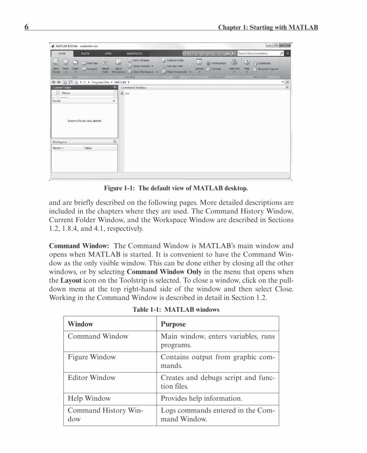
It is assumed that the software is installed on the computer, and that the usercan start the program. Once the program starts, the MATLAB desktop windowopens with the default layout, Figure 1-1. The layout has a Toolstrip at the top,the Current Folder Toolbar below it, and four windows underneath. At the topof the Toolstrip there are three tabs: HOME, PLOTS, and APPS. Clicking onthe tabs changes the icons in the Toolstrip. Commonly, MATLAB is used withthe HOME tab selected. The associated icons are used for executing variouscommands, as explained later in this chapter. The PLOTS tab can be used tocreate plots, as explained in Chapter 5 (Section 5.12), and the APPS tab can beused for opening additional applications and Toolboxes of MATLAB.
The default layoutThe default layout (Figure 1-1) consists of the following four windows that aredisplayed under the Toolstrip: the Command Window (the larger window), theCurrent Folder Window (on the top left), the Details Window and the Work-space Window (on the bottom lest). A list of several MATLAB windows andtheir purposes is given in Table 1-1.
Four of the windows—the Command Window, the Figure Window, the Edi-tor Window, and the Help Window—are used extensively throughout the book
6 Chapter 1: Starting with MATLAB
and are briefly described on the following pages. More detailed descriptions areincluded in the chapters where they are used. The Command History Window,Current Folder Window, and the Workspace Window are described in Sections1.2, 1.8.4, and 4.1, respectively.
Command Window: The Command Window is MATLAB’s main window andopens when MATLAB is started. It is convenient to have the Command Win-dow as the only visible window. This can be done either by closing all the otherwindows, or by selecting Command Window Only in the menu that opens whenthe Layout icon on the Toolstrip is selected. To close a window, click on the pull-down menu at the top right-hand side of the window and then select Close.Working in the Command Window is described in detail in Section 1.2.
Figure 1-1: The default view of MATLAB desktop.
Table 1-1: MATLAB windows
Window Purpose
Command Window Main window, enters variables, runsprograms.
Figure Window Contains output from graphic com-mands.
Editor Window Creates and debugs script and func-tion files.
Help Window Provides help information.
Command History Win-dow
Logs commands entered in the Com-mand Window.

1.1 Starting MATLAB, MATLAB Windows 7
Figure Window: The Figure Window opens automatically when graphics com-mands are executed, and contains graphs created by these commands. An exam-ple of a Figure Window is shown in Figure 1-2. A more detailed description ofthis window is given in Chapter 5.
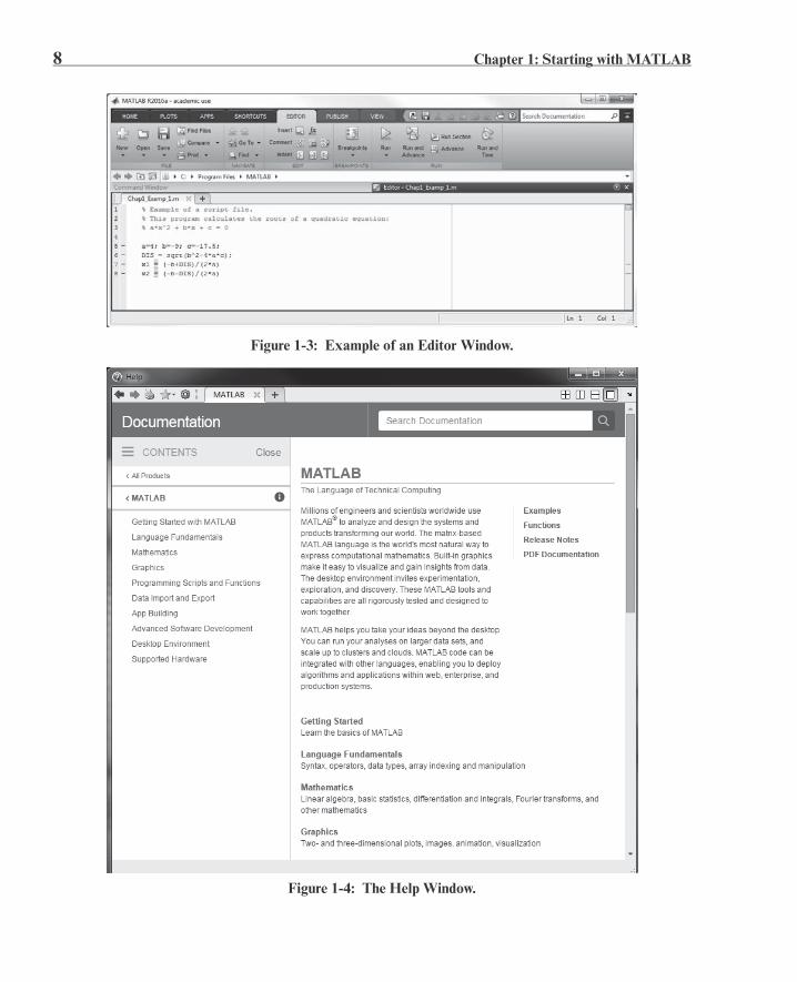
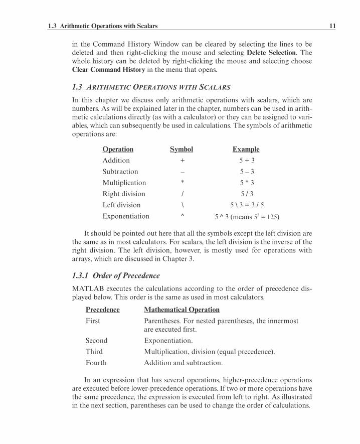
Editor Window: The Editor Window is used for writing and editing programs.This window is opened by clicking on the New Script icon in the Toolstrip, or byclicking on the New icon and then selecting Script from the menu that opens. Anexample of an Editor Window is shown in Figure 1-3. More details on the Edi-tor Window are given in Section 1.8.2, where it is used for writing script files,and in Chapter 7, where it is used to write function files.Help Window: The Help Window contains help information. This window canbe opened from the Help icon in the Toolstrip of the Command Window or thetoolbar of any MATLAB window. The Help Window is interactive and can beused to obtain information on any feature of MATLAB. Figure 1-4 shows anopen Help Window.
When MATLAB is started for the first time, the screen looks like thatshown in Figure 1-1. For most beginners it is probably more convenient to close
Workspace Window Provides information about the vari-ables that are stored.
Current Folder Window Shows the files in the current folder.
Figure 1-2: Example of a Figure Window.
Table 1-1: MATLAB windows
Window Purpose
8 Chapter 1: Starting with MATLAB
Figure 1-3: Example of an Editor Window.
Figure 1-4: The Help Window.

1.2 Working in the Command Window 9
all the windows except the Command Window. The closed windows can bereopened by selecting them from the layout icon in the Toolstrip. The windowsshown in Figure 1-1 can be displayed by clicking on the layout icon and selectingDefault in the menu that opens. The various windows in Figure 1-1 are dockedto the desktop. A window can be undocked (become a separate, independentwindow) by dragging it out. An independent window can be redocked by click-ing on the pull-down menu at the top right-hand side of the window and thenselecting Dock.
1.2 WORKING IN THE COMMAND WINDOW
The Command Window is MATLAB’s main window and can be used for execut-ing commands, opening other windows, running programs written by the user,and managing the software. An example of the Command Window, with severalsimple commands that will be explained later in this chapter, is shown in Figure1-5.
Notes for working in the Command Window:
• To type a command, the cursor must be placed next to the command prompt (>> ).
• Once a command is typed and the Enter key is pressed, the command is exe-cuted. However, only the last command is executed. Everything executed previ-ously (that might be still displayed) is unchanged.
• Several commands can be typed in the same line. This is done by typing acomma between the commands. When the Enter key is pressed, the commandsare executed in order from left to right.
• It is not possible to go back to a previous line that is displayed in the Command
Figure 1-5: The Command Window.
To type a command the cursor is placednext to the command prompt ( >> ).

10 Chapter 1: Starting with MATLAB
Window, make a correction, and then re-execute the command.
• A previously typed command can be recalled to the command prompt with theup-arrow key ( ). When the command is displayed at the command prompt, itcan be modified if needed and then executed. The down-arrow key ( ) can beused to move down the list of previously typed commands.
• If a command is too long to fit in one line, it can be continued to the next line bytyping three periods … (called an ellipsis) and pressing the Enter key. The con-tinuation of the command is then typed in the new line. The command can con-tinue line after line up to a total of 4,096 characters.
The semicolon ( ; ):When a command is typed in the Command Window and the Enter key ispressed, the command is executed. Any output that the command generates isdisplayed in the Command Window. If a semicolon ( ; ) is typed at the end of acommand, the output of the command is not displayed. Typing a semicolon isuseful when the result is obvious or known, or when the output is very large.
If several commands are typed in the same line, the output from any of thecommands will not be displayed if a semicolon instead of a comma is typedbetween the commands.Typing %:When the symbol % (percent) is typed at the beginning of a line, the line is desig-nated as a comment. This means that when the Enter key is pressed the line isnot executed. The % character followed by text (comment) can also be typedafter a command (in the same line). This has no effect on the execution of thecommand.
Usually there is no need for comments in the Command Window. Com-ments, however, are frequently used in a program to add descriptions or toexplain the program (see Chapters 4 and 6).The clc command:The clc command (type clc and press Enter) clears the Command Window.After typing in the Command Window for a while, the display may become verylong. Once the clc command is executed, a clear window is displayed. Thecommand does not change anything that was done before. For example, if somevariables were defined previously (see Section 1.6), they still exist and can beused. The up-arrow key can also be used to recall commands that were typedbefore.The Command History Window:The Command History Window lists the commands that have been entered inthe Command Window. This includes commands from previous sessions. Acommand in the Command History Window can be used again in the Com-mand Window. By double-clicking on the command, the command is reenteredin the Command Window and executed. It is also possible to drag the commandto the Command Window, make changes if needed, and then execute it. The list
1.3 Arithmetic Operations with Scalars 11
in the Command History Window can be cleared by selecting the lines to bedeleted and then right-clicking the mouse and selecting Delete Selection. Thewhole history can be deleted by right-clicking the mouse and selecting chooseClear Command History in the menu that opens.
1.3 ARITHMETIC OPERATIONS WITH SCALARS
In this chapter we discuss only arithmetic operations with scalars, which arenumbers. As will be explained later in the chapter, numbers can be used in arith-metic calculations directly (as with a calculator) or they can be assigned to vari-ables, which can subsequently be used in calculations. The symbols of arithmeticoperations are:
It should be pointed out here that all the symbols except the left division arethe same as in most calculators. For scalars, the left division is the inverse of theright division. The left division, however, is mostly used for operations witharrays, which are discussed in Chapter 3.
1.3.1 Order of Precedence
MATLAB executes the calculations according to the order of precedence dis-played below. This order is the same as used in most calculators.
In an expression that has several operations, higher-precedence operationsare executed before lower-precedence operations. If two or more operations havethe same precedence, the expression is executed from left to right. As illustratedin the next section, parentheses can be used to change the order of calculations.
Operation Symbol Example
Addition + 5 + 3
Subtraction – 5 – 3
Multiplication * 5 * 3
Right division / 5 / 3
Left division \ 5 \ 3 = 3 / 5
Exponentiation ^ 5 ^ 3 (means 53 = 125)
Precedence Mathematical Operation
First Parentheses. For nested parentheses, the innermostare executed first.
Second Exponentiation.
Third Multiplication, division (equal precedence).
Fourth Addition and subtraction.
12 Chapter 1: Starting with MATLAB
1.3.2 Using MATLAB as a Calculator
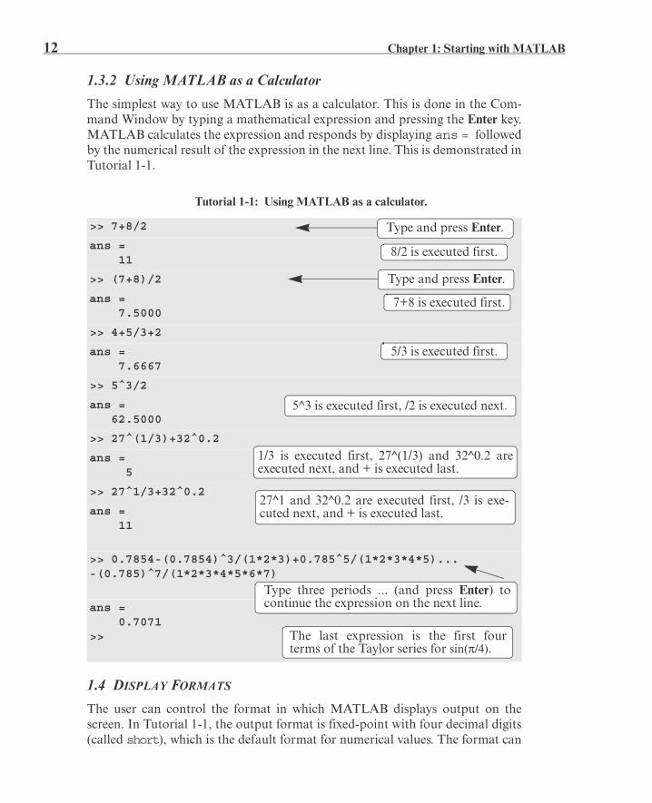
The simplest way to use MATLAB is as a calculator. This is done in the Com-mand Window by typing a mathematical expression and pressing the Enter key.MATLAB calculates the expression and responds by displaying ans = followedby the numerical result of the expression in the next line. This is demonstrated inTutorial 1-1.
1.4 DISPLAY FORMATS
The user can control the format in which MATLAB displays output on thescreen. In Tutorial 1-1, the output format is fixed-point with four decimal digits(called short), which is the default format for numerical values. The format can
Tutorial 1-1: Using MATLAB as a calculator.
>> 7+8/2
ans = 11
>> (7+8)/2
ans = 7.5000
>> 4+5/3+2
ans = 7.6667
>> 5^3/2
ans = 62.5000
>> 27^(1/3)+32^0.2
ans = 5
>> 27^1/3+32^0.2
ans = 11
>> 0.7854-(0.7854)^3/(1*2*3)+0.785^5/(1*2*3*4*5)...-(0.785)^7/(1*2*3*4*5*6*7)
ans = 0.7071>>
Type and press Enter.
8/2 is executed first.
Type and press Enter.
7+8 is executed first.
5/3 is executed first.
5^3 is executed first, /2 is executed next.
1/3 is executed first, 27^(1/3) and 32^0.2 areexecuted next, and + is executed last.
27^1 and 32^0.2 are executed first, /3 is exe-cuted next, and + is executed last.
Type three periods ... (and press Enter) tocontinue the expression on the next line.
The last expression is the first fourterms of the Taylor series for sin( /4).

1.4 Display Formats 13
be changed with the format command. Once the format command is entered,all the output that follows is displayed in the specified format. Several of theavailable formats are listed and described in Table 1-2.
MATLAB has several other formats for displaying numbers. Details ofthese formats can be obtained by typing help format in the Command Win-dow. The format in which numbers are displayed does not affect how MATLABcomputes and saves numbers.
Table 1-2: Display formats
Command Description Example
format short Fixed-point with 4 decimal digits for:
Otherwise display format short e.
>> 290/7ans = 41.4286
format long Fixed-point with 15 deci-mal digits for:
Otherwise display format long e.
>> 290/7ans = 41.428571428571431
format short e Scientific notation with 4 decimal digits.
>> 290/7ans = 4.1429e+001
format long e Scientific notation with 15 decimal digits.
>> 290/7ans = 4.142857142857143e+001
format short g Best of 5-digit fixed or floating point.
>> 290/7ans = 41.429
format long g Best of 15-digit fixed or floating point.
>> 290/7ans = 41.4285714285714
format bank Two decimal digits. >> 290/7ans = 41.43
format compact Eliminates blank lines to allow more lines with informa-tion displayed on the screen.
format loose Adds blank lines (opposite of compact).
0.001 number 1000
0.001 number 100

14 Chapter 1: Starting with MATLAB
1.5 ELEMENTARY MATH BUILT-IN FUNCTIONS
In addition to basic arithmetic operations, expressions in MATLAB can includefunctions. MATLAB has a very large library of built-in functions. A functionhas a name and an argument in parentheses. For example, the function that cal-culates the square root of a number is sqrt(x). Its name is sqrt, and theargument is x. When the function is used, the argument can be a number, a vari-able that has been assigned a numerical value (explained in Section 1.6), or acomputable expression that can be made up of numbers and/or variables. Func-tions can also be included in arguments, as well as in expressions. Tutorial 1-2shows examples of using the function sqrt(x) when MATLAB is used as acalculator with scalars.
Some commonly used elementary MATLAB mathematical built-in func-tions are given in Tables 1-3 through 1-5. A complete list of functions organizedby category can be found in the Help Window.
Tutorial 1-2: Using the sqrt built-in function.
>> sqrt(64)
ans = 8
>> sqrt(50+14*3)
ans = 9.5917
>> sqrt(54+9*sqrt(100))
ans = 12
>> (15+600/4)/sqrt(121)
ans = 15>>
Table 1-3: Elementary math functions
Function Description Example
sqrt(x) Square root. >> sqrt(81)ans = 9
nthroot(x,n) Real nth root of a real number x. (If x is negative n must be an odd integer.)
>> nthroot(80,5)ans = 2.4022
exp(x) Exponential . >> exp(5)ans = 148.4132
Argument is a number.
Argument is an expression.
Argument includes a function.
Function is included in an expression.
ex
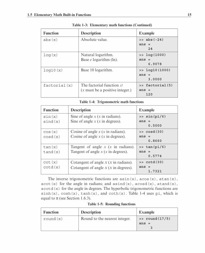
1.5 Elementary Math Built-in Functions 15
The inverse trigonometric functions are asin(x), acos(x), atan(x),acot(x) for the angle in radians; and asind(x), acosd(x), atand(x),acotd(x) for the angle in degrees. The hyperbolic trigonometric functions aresinh(x), cosh(x), tanh(x), and coth(x). Table 1-4 uses pi, which isequal to (see Section 1.6.3).
abs(x) Absolute value. >> abs(-24)ans = 24
log(x) Natural logarithm.Base e logarithm (ln).
>> log(1000)ans = 6.9078
log10(x) Base 10 logarithm. >> log10(1000)ans = 3.0000
factorial(x) The factorial function x! (x must be a positive integer.)
>> factorial(5)ans = 120
Table 1-4: Trigonometric math functions
Function Description Example
sin(x)sind(x)
Sine of angle x (x in radians).Sine of angle x (x in degrees).
>> sin(pi/6)ans = 0.5000
cos(x)cosd(x)
Cosine of angle x (x in radians).Cosine of angle x (x in degrees).
>> cosd(30)ans = 0.8660
tan(x)tand(x)
Tangent of angle x (x in radians).Tangent of angle x (x in degrees).
>> tan(pi/6)ans = 0.5774
cot(x)cotd(x)
Cotangent of angle x (x in radians).Cotangent of angle x (x in degrees).
>> cotd(30)ans = 1.7321
Table 1-5: Rounding functions
Function Description Example
round(x) Round to the nearest integer. >> round(17/5)ans = 3
Table 1-3: Elementary math functions (Continued)
Function Description Example

16 Chapter 1: Starting with MATLAB
1.6 DEFINING SCALAR VARIABLES
A variable is a name made of a letter or a combination of several letters (anddigits) that is assigned a numerical value. Once a variable is assigned a numericalvalue, it can be used in mathematical expressions, in functions, and in any MAT-LAB statements and commands. A variable is actually a name of a memorylocation. When a new variable is defined, MATLAB allocates an appropriatememory space where the variable’s assignment is stored. When the variable isused the stored data is used. If the variable is assigned a new value the content ofthe memory location is replaced. (In Chapter 1 we consider only variables thatare assigned numerical values that are scalars. Assigning and addressing vari-ables that are arrays is discussed in Chapter 2.)
1.6.1 The Assignment Operator
In MATLAB the = sign is called the assignment operator. The assignmentoperator assigns a value to a variable.
• The left-hand side of the assignment operator can include only one variablename. The right-hand side can be a number, or a computable expression that caninclude numbers and/or variables that were previously assigned numerical val-ues. When the Enter key is pressed the numerical value of the right-hand side isassigned to the variable, and MATLAB displays the variable and its assignedvalue in the next two lines.
fix(x) Round toward zero. >> fix(13/5)ans = 2
ceil(x) Round toward infinity. >> ceil(11/5)ans = 3
floor(x) Round toward minus infinity. >> floor(-9/4)ans = -3
rem(x,y) Returns the remainder after xis divided by y.
>> rem(13,5)ans = 3
sign(x) Signum function. Returns 1 if, –1 if , and 0 if
.
>> sign(5)ans = 1
Table 1-5: Rounding functions (Continued)
Function Description Example
x 0> x 0<x 0=
Variable_name = A numerical value, or a computable expression
1.6 Defining Scalar Variables 17
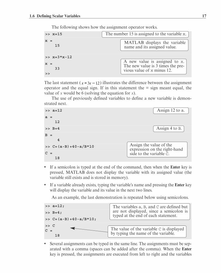
The following shows how the assignment operator works.
The last statement ( ) illustrates the difference between the assignmentoperator and the equal sign. If in this statement the = sign meant equal, thevalue of x would be 6 (solving the equation for x).
The use of previously defined variables to define a new variable is demon-strated next.
• If a semicolon is typed at the end of the command, then when the Enter key ispressed, MATLAB does not display the variable with its assigned value (thevariable still exists and is stored in memory).
• If a variable already exists, typing the variable’s name and pressing the Enter keywill display the variable and its value in the next two lines.
As an example, the last demonstration is repeated below using semicolons.
• Several assignments can be typed in the same line. The assignments must be sep-arated with a comma (spaces can be added after the comma). When the Enterkey is pressed, the assignments are executed from left to right and the variables
>> x=15
x = 15
>> x=3*x-12
x = 33>>
>> a=12
a = 12
>> B=4
B = 4
>> C=(a-B)+40-a/B*10
C = 18
>> a=12;
>> B=4;
>> C=(a-B)+40-a/B*10;
>> CC = 18
The number 15 is assigned to the variable x.
MATLAB displays the variablename and its assigned value.
A new value is assigned to x.The new value is 3 times the pre-vious value of x minus 12.
Assign 12 to a.
Assign 4 to B.
Assign the value of the expression on the right-hand side to the variable C.
The variables a, B, and C are defined butare not displayed, since a semicolon istyped at the end of each statement.
The value of the variable C is displayedby typing the name of the variable.
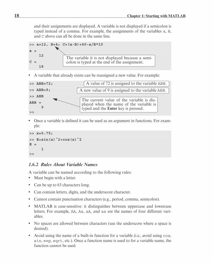
18 Chapter 1: Starting with MATLAB
and their assignments are displayed. A variable is not displayed if a semicolon istyped instead of a comma. For example, the assignments of the variables a, B,and C above can all be done in the same line.
• A variable that already exists can be reassigned a new value. For example:
• Once a variable is defined it can be used as an argument in functions. For exam-ple:
1.6.2 Rules About Variable Names
A variable can be named according to the following rules:• Must begin with a letter.
• Can be up to 63 characters long.
• Can contain letters, digits, and the underscore character.
• Cannot contain punctuation characters (e.g., period, comma, semicolon).
• MATLAB is case-sensitive: it distinguishes between uppercase and lowercaseletters. For example, AA, Aa, aA, and aa are the names of four different vari-ables.
• No spaces are allowed between characters (use the underscore where a space isdesired).
• Avoid using the name of a built-in function for a variable (i.e., avoid using cos,sin, exp, sqrt, etc.). Once a function name is used to for a variable name, thefunction cannot be used.
>> a=12, B=4; C=(a-B)+40-a/B*10
a = 12
C = 18
>> ABB=72;
>> ABB=9;
>> ABB
ABB = 9>>
>> x=0.75;
>> E=sin(x)^2+cos(x)^2E = 1>>
The variable B is not displayed because a semi-colon is typed at the end of the assignment.
A value of 72 is assigned to the variable ABB.
A new value of 9 is assigned to the variable ABB.
The current value of the variable is dis-played when the name of the variable istyped and the Enter key is pressed.

1.7 Useful Commands for Managing Variables 19
1.6.3 Predefined Variables and Keywords
There are 20 words, called keywords, that are reserved by MATLAB for variouspurposes and cannot be used as variable names. These words are:
break case catch classdef continue else elseif end forfunction global if otherwise parfor persistent returnspmd switch try while
When typed, these words appear in blue. An error message is displayed if theuser tries to use a keyword as a variable name. (The keywords can be displayedby typing the command iskeyword.)
A number of frequently used variables are already defined when MATLABis started. Some of the predefined variables are:
ans A variable that has the value of the last expression that was not assignedto a specific variable (see Tutorial 1-1). If the user does not assign thevalue of an expression to a variable, MATLAB automatically stores theresult in ans.
pi The number .eps The smallest difference between two numbers. Equal to 2^(–52), which is
approximately 2.2204e–016.inf Used for infinity.
i Defined as , which is: 0 + 1.0000i.j Same as i.NaN Stands for Not-a-Number. Used when MATLAB cannot determine a
valid numeric value. Example: 0/0.
The predefined variables can be redefined to have any other value. The vari-ables pi, eps, and inf, are usually not redefined since they are frequently usedin many applications. Other predefined variables, such as i and j, are sometimeredefined (commonly in association with loops) when complex numbers are notinvolved in the application.
1.7 USEFUL COMMANDS FOR MANAGING VARIABLES
The following are commands that can be used to eliminate variables or to obtaininformation about variables that have been created. When these commands aretyped in the Command Window and the Enter key is pressed, either they pro-vide information, or they perform a task as specified below.
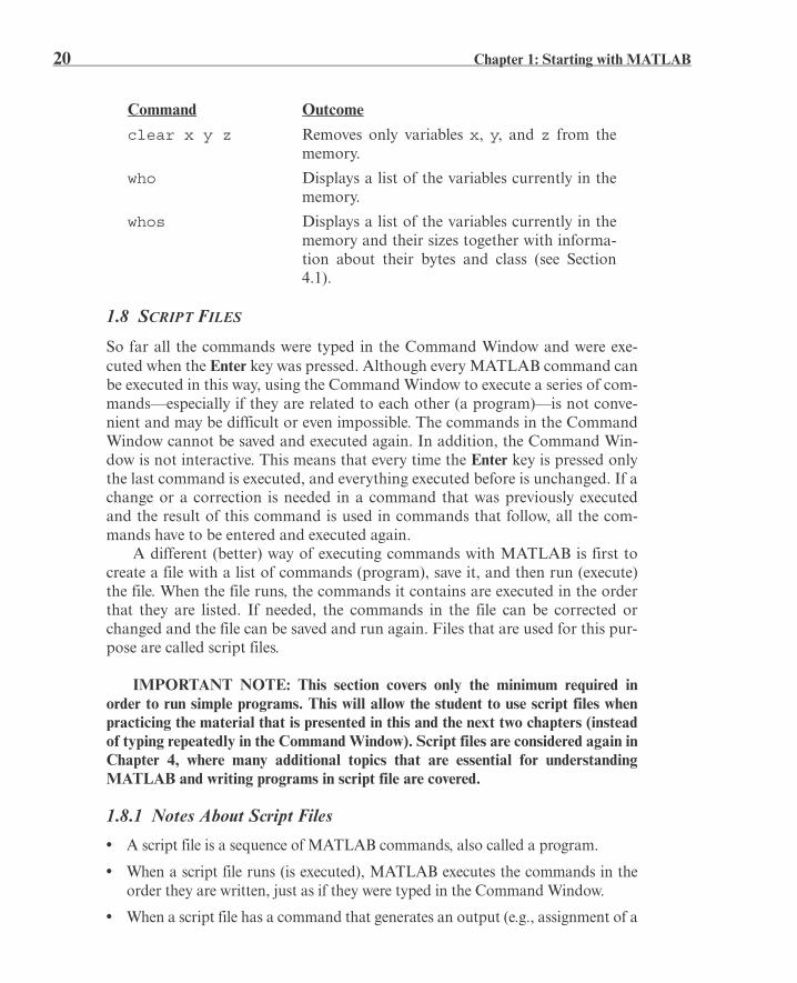
Command Outcome
clear Removes all variables from the memory.
20 Chapter 1: Starting with MATLAB
1.8 SCRIPT FILES
So far all the commands were typed in the Command Window and were exe-cuted when the Enter key was pressed. Although every MATLAB command canbe executed in this way, using the Command Window to execute a series of com-mands—especially if they are related to each other (a program)—is not conve-nient and may be difficult or even impossible. The commands in the CommandWindow cannot be saved and executed again. In addition, the Command Win-dow is not interactive. This means that every time the Enter key is pressed onlythe last command is executed, and everything executed before is unchanged. If achange or a correction is needed in a command that was previously executedand the result of this command is used in commands that follow, all the com-mands have to be entered and executed again.
A different (better) way of executing commands with MATLAB is first tocreate a file with a list of commands (program), save it, and then run (execute)the file. When the file runs, the commands it contains are executed in the orderthat they are listed. If needed, the commands in the file can be corrected orchanged and the file can be saved and run again. Files that are used for this pur-pose are called script files.
IMPORTANT NOTE: This section covers only the minimum required inorder to run simple programs. This will allow the student to use script files whenpracticing the material that is presented in this and the next two chapters (insteadof typing repeatedly in the Command Window). Script files are considered again inChapter 4, where many additional topics that are essential for understandingMATLAB and writing programs in script file are covered.
1.8.1 Notes About Script Files
• A script file is a sequence of MATLAB commands, also called a program.
• When a script file runs (is executed), MATLAB executes the commands in theorder they are written, just as if they were typed in the Command Window.
• When a script file has a command that generates an output (e.g., assignment of a
clear x y z Removes only variables x, y, and z from thememory.
who Displays a list of the variables currently in thememory.
whos Displays a list of the variables currently in thememory and their sizes together with informa-tion about their bytes and class (see Section4.1).
Command Outcome
1.8 Script Files 21
value to a variable without a semicolon at the end), the output is displayed in theCommand Window.
• Using a script file is convenient because it can be edited (corrected or otherwisechanged) and executed many times.
• Script files can be typed and edited in any text editor and then pasted into theMATLAB editor.
• Script files are also called M-files because the extension .m is used when they aresaved.
1.8.2 Creating and Saving a Script File
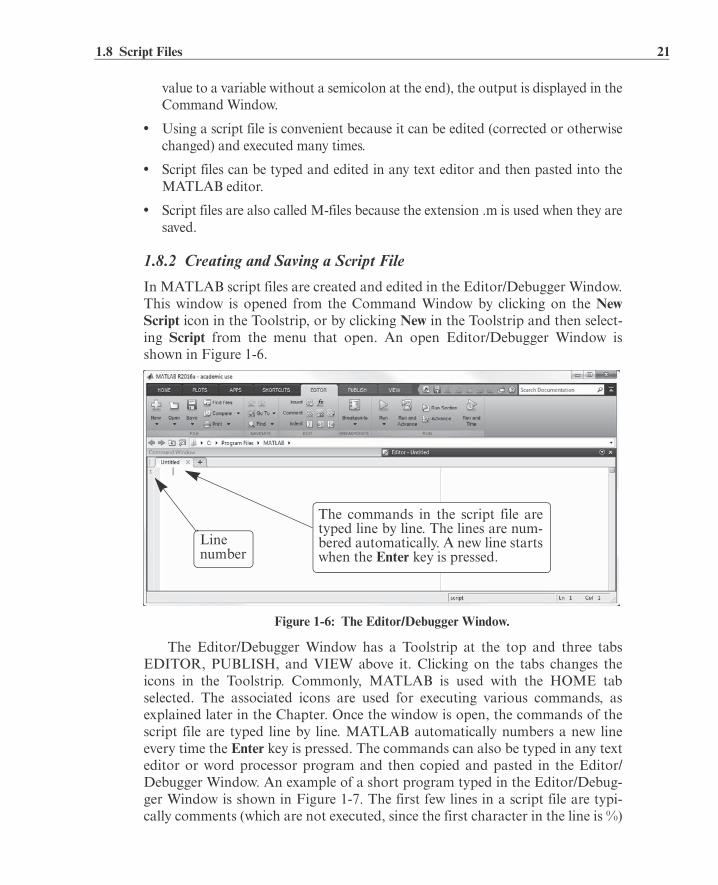
In MATLAB script files are created and edited in the Editor/Debugger Window.This window is opened from the Command Window by clicking on the NewScript icon in the Toolstrip, or by clicking New in the Toolstrip and then select-ing Script from the menu that open. An open Editor/Debugger Window isshown in Figure 1-6.
The Editor/Debugger Window has a Toolstrip at the top and three tabsEDITOR, PUBLISH, and VIEW above it. Clicking on the tabs changes theicons in the Toolstrip. Commonly, MATLAB is used with the HOME tabselected. The associated icons are used for executing various commands, asexplained later in the Chapter. Once the window is open, the commands of thescript file are typed line by line. MATLAB automatically numbers a new lineevery time the Enter key is pressed. The commands can also be typed in any texteditor or word processor program and then copied and pasted in the Editor/Debugger Window. An example of a short program typed in the Editor/Debug-ger Window is shown in Figure 1-7. The first few lines in a script file are typi-cally comments (which are not executed, since the first character in the line is %)
Figure 1-6: The Editor/Debugger Window.
The commands in the script file aretyped line by line. The lines are num-bered automatically. A new line startswhen the Enter key is pressed.
Linenumber

22 Chapter 1: Starting with MATLAB
that describe the program written in the script file.
Before a script file can be executed it has to be saved. This is done by click-ing Save in the Toolstrip and selecting Save As... from the menu that opens.When saved, MATLAB adds the extension .m to the name. The rules for nam-ing a script file follow the rules of naming a variable (must begin with a letter,can include digits and underscore, no spaces, and up to 63 characters long). Thenames of user-defined variables, predefined variables, and MATLAB commandsor functions should not be used as names of script files.
1.8.3 Running (Executing) a Script File
A script file can be executed either directly from the Editor Window by clickingon the Run icon (see Figure 1-7) or by typing the file name in the CommandWindow and then pressing the Enter key. For a file to be executed, MATLABneeds to know where the file is saved. The file will be executed if the folder wherethe file is saved is the current folder of MATLAB or if the folder is listed in thesearch path, as explained next.
1.8.4 Current Folder
The current folder is shown in the “Current Folder” field in the desktop toolbarof the Command Window, as shown in Figure 1-8. If an attempt is made to exe-cute a script file by clicking on the Run icon (in the Editor Window) when thecurrent folder is not the folder where the script file is saved, then the promptshown in Figure 1-9 opens. The user can then change the current folder to thefolder where the script file is saved, or add it to the search path. Once two ormore different current folders are used in a session, it is possible to switch fromone to another in the Current Folder field in the Command Window. The cur-
Figure 1-7: A program typed in the Editor/Debugger Window.
Comments.
Define threevariables.
Calculating the two roots.
The Run icon.

1.8 Script Files 23
rent folder can also be changed in the Current Folder Window, shown in Figure1-10, which can be opened from the Desktop menu. The Current Folder can bechanged by choosing the drive and folder where the file is saved.
Figure 1-8: The Current folder field in the Command Window.
Figure 1-9: Changing the current directory.
Figure 1-10: The Current Folder Window.
The current folder is shown here.
Current foldershown here.
Click here tochange thefolder.
Click here tobrowse for afolder.
Click here togo up onelevel in thefile system.

24 Chapter 1: Starting with MATLAB
An alternative simple way to change the current folder is to use the cd com-mand in the Command Window. To change the current folder to a differentdrive, type cd, space, and then the name of the directory followed by a colon :and press the Enter key. For example, to change the current folder to drive E(e.g., the flash drive) type cd E:. If the script file is saved in a folder within adrive, the path to that folder has to be specified. This is done by typing the pathas a string in the cd command. For example, cd('E:\Chapter 1') sets thepath to the folder Chapter 1 in drive F. The following example shows how thecurrent folder is changed to be drive E. Then the script file from Figure 1-7,which was saved in drive E as ProgramExample.m, is executed by typing thename of the file and pressing the Enter key.
1.9 EXAMPLES OF MATLAB APPLICATIONS
Sample Problem 1-1: Trigonometric identity
A trigonometric identity is given by:
Verify that the identity is correct by calculating each side of the equation, substi-
tuting .
Solution
The problem is solved by typing the following commands in the Command Win-dow.
>> cd('E:\Chapter 1')
>> Chap1_Examp1
x1 = 3.5000x2 = -1.2500
>> x=pi/5;
>> LHS=cos(x/2)^2
LHS = 0.9045
>> RHS=(tan(x)+sin(x))/(2*tan(x))
RHS = 0.9045
The current directory is changed to drive E.
The script file is executed by typing thename of the file and pressing the Enter key.
The output generated by the script file (the roots x1and x2) is displayed in the Command Window.
x2---cos2 xtan xsin+
2 xtan-------------------------------=
x5---=
Define x.
Calculate the left-hand side.
Calculate the right-hand side.

1.9 Examples of MATLAB Applications 25
Sample Problem 1-2: Geometry and trigonometry
Four circles are placed as shown in the figure.At each point where two circles are in contact,they are tangent to each other. Determine thedistance between the centers C2 and C4.The radii of the circles are:
mm, mm, mm, andmm.
Solution
The lines that connect the centers of the circlescreate four triangles. In two of the triangles, C1C2C3and C1C3C4, the lengths of all the sides are known.This information is used to calculate the angles 1 and
2 in these triangles by using the law of cosines. Forexample, 1 is calculated from:
Next, the length of the side C2C4 is calculated byconsidering the triangle C1C2C4. This is done, again, by using the law ofcosines (the lengths C1C2 and C1C4 are known and the angle 3 is the sum of theangles 1 and 2).
The problem is solved by writing the following program in a script file:
When the script file is executed, the following (the value of the variable C2C4) isdisplayed in the Command Window:
% Solution of Sample Problem 1-2
R1=16; R2=6.5; R3=12; R4=9.5;
C1C2=R1+R2; C1C3=R1+R3; C1C4=R1+R4;
C2C3=R2+R3; C3C4=R3+R4;
Gama1=acos((C1C2^2+C1C3^2-C2C3^2)/(2*C1C2*C1C3));
Gama2=acos((C1C3^2+C1C4^2-C3C4^2)/(2*C1C3*C1C4));
Gama3=Gama1+Gama2;
C2C4=sqrt(C1C2^2+C1C4^2-2*C1C2*C1C4*cos(Gama3))
C2C4 = 33.5051
C1
C2
C3
C4
Define the R’s.
Calculate the lengths of the sides.
Calculate 1, 2, and 3.
Calculate the length of side C2C4.

26 Chapter 1: Starting with MATLAB
Sample Problem 1-3: Heat transfer
An object with an initial temperature of that is placed at time t = 0 inside achamber that has a constant temperature of will experience a temperaturechange according to the equation
where T is the temperature of the object at time t, and k is a constant. A sodacan at a temperature of 120° F (after being left in the car) is placed inside arefrigerator where the temperature is 38° F. Determine, to the nearest degree, thetemperature of the can after three hours. Assume k = 0.45. First define all of thevariables and then calculate the temperature using one MATLAB command.
Solution
The problem is solved by typing the following commands in the Command Win-dow.
Sample Problem 1-4: Compounded interest
The balance B of a savings account after t years when a principal P is invested atan annual interest rate r and the interest is compounded n times a year is givenby:
(1)
If the interest is compounded yearly, the balance is given by:
(2)Suppose $5,000 is invested for 17 years in one account for which the interest iscompounded yearly. In addition, $5,000 is invested in a second account in whichthe interest is compounded monthly. In both accounts the interest rate is 8.5%.Use MATLAB to determine how long (in years and months) it would take forthe balance in the second account to be the same as the balance of the firstaccount after 17 years.
Solution
Follow these steps:(a) Calculate B for $5,000 invested in a yearly compounded interest accountafter 17 years using Equation (2).(b) Calculate t for the B calculated in part (a), from the monthly compounded
>> Ts=38; T0=120; k=0.45; t=3;
>> T=round(Ts+(T0-Ts)*exp(-k*t))
T = 59
Round to the nearest integer.

1.10 Problems 27
interest formula, Equation (1).(c) Determine the number of years and months that correspond to t.
The problem is solved by writing the following program in a script file:
When the script file is executed, the following (the values of the variables B, t,years, and months) is displayed in the Command Window:
1.10 PROBLEMS
The following problems can be solved by writing commands in the CommandWindow or by writing a program in a script file and then executing the file.
1. Calculate:
(a) (b)
2. Calculate:
(a) (b)
% Solution of Sample Problem 1-4
P=5000; r=0.085; ta=17; n=12;
B=P*(1+r)^ta
t=log(B/P)/(n*log(1+r/n))
years=fix(t)
months=ceil((t-years)*12)
>> format short gB = 20011
t = 16.374
years = 16
months = 5
Step (a): Calculate B from Eq. (2).
Step (b): Solve Eq. (1) for t, and calculate t.
Step (c): Determine the number of years.
Determine the number of months.
The values of the variables B, t,years, and months are displayed(since a semicolon was not typed atthe end of any of the commands thatcalculate the values).

28 Chapter 1: Starting with MATLAB
3. Calculate:
(a) (b)
4. Calculate:
(a) (b)
5. Calculate:
(a) (b)
6. Define the variable z as z = 4.5; then evaluate:
(a) (b)
7. Define the variable t as t = 3.2; then evaluate:
(a) (b)
8. Define the variables x and y as x = 6.5 and y = 3.8; then evaluate:
(a) (b)
9. Define the variables a, b, c, and d as:
, , , and ; then evaluate:
(a) (b)
10. Two trigonometric identities are given by:
(a) (b)
For each part, verify that the identity is correct by calculating the values ofthe left and right sides of the equation, substituting .
11. Two trigonometric identities are given by:
(a) (b)
For each part, verify that the identity is correct by calculating the values ofthe left and right sides of the equation, substituting .

1.10 Problems 29
12. Define two variables: alpha = /8, and beta = /6. Using these variables, showthat the following trigonometric identity is correct by calculating the valuesof the left and right sides of the equation.
13. Given: . Use MATLAB to calculate the
following definite integral: .
14. A rectangular box has the dimensions shown.(a) Determine the angle BAC to the nearest
degree.(b) Determine the area of the triangle ABC to
the nearest tenth of a centimeter.
Law of cosines: Heron’s formula for triangular area:
, where .
15. The arc length of a segment of a parabola ABC isgiven by:
Determine LABC if a=8 in. and h=13 in.
16. The three shown circles, with radius 15 in.,10.5 in., and 4.5 in., are tangent to each other.
(a) Calculate the angle (in degrees) byusing the law of cosines.
(Law of cosines: ) (b) Calculate the angles and (in degrees)
using the law of sines.(c) Check that the sum of the angles is 180º.
17. A frustum of cone is filled with ice cream such thatthe portion above the cone is a hemisphere. Definethe variables di=1.25 in., d0=2.25 in., h=2 in., anddetermine the volume of the ice cream.
43 cm
16 cm
23 cm
A
BC
h
a x
y
A
B
Ca
di
do
h

30 Chapter 1: Starting with MATLAB
18. In the triangle shown in., in., andin. Define a, b, and c as variables, and then:
(a) Calculate the angles , , and by substituting thevariables in the law of cosines.
(Law of cosines: )(b) Verify the law of tangents by substituting the
results into the right and left sides of:
law of tangents:
19. For the triangle shown, , , and its perimeter is mm.Define , , and p, as variables, and then:(a) Calculate the triangle sides (Use the law of
sines). (b) Calculate the radius r of the circle inscribed in
the triangle using the formula:
where .
20. The distance d from a point P to theline that passes through the two points A
and B can be calculated by where r is the distance between the
points A and B, given by
and S is thearea of the triangle defined by the three points cal-
culated by where
. Determine the distance ofpoint P from the line that passes through point Aand point B . First define the variables xP, yP, zP, xA, yA, zA, xB,yB, and zB, and then use the variable to calculate s1, s2, s3, and r. Finally cal-culate S and d.
x
y
z
A
B
P

1.10 Problems 31
21. The perimeter of an ellipse can be approximatedby:
Calculate the perimeter of an ellipse with
in. and in.
22. A total of 4217 eggs have to be packed in boxes that can hold 36 eggs each.By typing one line (command) in the Command Window, calculate howmany eggs will remain unpacked if every box that is used has to be full.(Hint: Use MATLAB built-in function fix.)
23. A total of 777 people have to be transported using buses that have 46 seatsand vans that have 12 seats. Calculate how many buses are needed if all thebuses have to be full, and how many seats will remain empty in the vans ifenough vans are used to transport all the people that did not fit into thebuses. (Hint: Use MATLAB built-in functions fix and ceil.)
24. Change the display to format long g. Assign the number 7E8/13 to avariable, and then use the variable in a mathematical expression to calculatethe following by typing one command: (a) Round the number to the nearest tenth.(b) Round the number to the nearest million.
25. The voltage difference Vab between points a
and b in the Wheatstone bridge circuit is givenby:
where and . Calculatethe Vab if V, , ,
, and .
26. The current in a series RCL circuit is givenby:
where . Calculate I for the circuit shown if the supply voltage is 80V, Hz, , H, and F.
b
ax
y
+V
R1 R2
R3R4
a b
V
R L C

32 Chapter 1: Starting with MATLAB
27. The monthly payment M of a mortgage P for n years with a fixed annualinterest rate r can be calculated by the formula:
Determine the monthly payment of a 30-year $450,000 mortgage with inter-est rate of 4.2% ( ). Define the variables P, r, and n and then usethem in the formula to calculate M.
28. The number of permutations of taking r objects out of n objects with-out repetition is given by:
(a) Determine how many six-letter passwords can be formed from the 26letters in the English alphabet if a letter can only be used once.
(b) How many passwords can be formed if the digits 0, 1, 2, ..., 9 can beused in addition to the letters.
29. The number of combinations of taking r objects out of n objects is givenby:
In the Powerball lottery game the player chooses five numbers from 1through 59, and then the Powerball number from 1 through 35.Determine how many combinations are possible by calculating . (Use the built-in function factorial.)
30. The equivalent resistance of two resistorsR1 and R2 connected in parallel is given by
. The equivalent resistance of
two resistors R1 and R2 connected in series
is given by . Determine theequivalent resistance of the four resistors in the circuit shown in the figure.
31. The output voltage Vout in the circuit shown is given
by (Millman’s theorem):
Calculate Vout given V, V, V,
,, ,, ,.
R1
Vout
R2 R3
V1 V2 V3

1.10 Problems 33
32. Radioactive decay of carbon-14 is used for estimating the age of organic
material. The decay is modeled with the exponential function ,where t is time, is the amount of material at , is the amountof material at time t, and k is a constant. Carbon-14 has a half-life ofapproximately 5,730 years. A sample taken from the ancient footprints ofAcahualinca in Nicaragua shows that 77.45% of the initial ( ) carbon-14 is present. Determine the estimated age of the footprint. Solve the prob-lem by writing a program in a script file. The program first determines theconstant k, then calculates t for , and finally rounds theanswer to the nearest year.
33. The greatest common divisor is the largest positive integer that divides thenumbers without a remainder. For example, the greatest common divisor of8 and 12 is 4. Use the MATLAB Help Window to find a MATLAB built-infunction that determines the greatest common divisor of two numbers. Thenuse the function to show that the greatest common divisor of: (a) 91 and 147 is 7. (b) 555 and 962 is 37.
34. The amount of energy E (in joules) that is released by an earthquake is givenby:
where M is the magnitude of the earthquake on the Richter scale. (a) Determine the energy that was released from the Anchorage earthquake
(1964, Alaska, USA), magnitude 9.2.(b) The energy released in Lisbon earthquake (Portugal) in 1755 was one-
half the energy released in the Anchorage earthquake. Determine themagnitude of the earthquake in Lisbon on the Richter scale.
35. According to the Doppler effect of light, the perceived wavelength of alight source with a wavelength of is given by:
where c is the speed of light (about m/s) and v is the speed theobserver moves toward the light source. Calculate the speed the observerhas to move in order to see a red light as green. Green wavelength is 530 nmand red wavelength is 630 nm.
36. Newton’s law of cooling gives the temperature T(t) of an object at time t interms of T0, its temperature at , and Ts, the temperature of the sur-roundings.
p

34 Chapter 1: Starting with MATLAB
A police officer arrives at a crime scene in a hotel room at 9:18 PM, wherehe finds a dead body. He immediately measures the body’s temperature andfinds it to be 79.5ºF. Exactly one hour later he measures the temperatureagain and finds it to be 78.0ºF. Determine the time of death, assuming thatvictim body temperature was normal (98.6ºF) prior to death and that theroom temperature was constant at 69ºF.
37. The velocity v and the falling distance d as a function of time of a skydiverthat experience the air resistance can be approximated by:
and
where kg/m is a constant, m is the skydiver mass, m/s2 is theacceleration due to gravity, and t is the time in seconds since the skydiverstarts falling. Determine the velocity and the falling distance at s for a95-kg skydiver
38. Use the Help Window to find a display format that displays the output as aratio of integers. For example, the number 3.125 will be displayed as 25/8.Change the display to this format and execute the following operations:
(a) (b)
39. Gosper’s approximation for factorials is given by:
Use the formula for calculating 19!. Compare the result with the true valueobtained with MATLAB’s built-in function factorial by calculating theerror (Error=(TrueVal-ApproxVal)/TrueVal).
40. According to Newton’s law of universal gravitation, the attraction force
between two bodies is given by:
where m1 and m2 are the masses of the bodies, r is the distance between the
bodies, and N-m2/kg2 is the universal gravitational constant.Determine how many times the attraction force between the sun and theEarth is larger than the attraction force between the Earth and the moon.The distance between the sun and Earth is m, the distance
between the moon and Earth is m, kg,
kg, and kg.

35
Chapter 2 Creating Arrays
The array is a fundamental form that MATLAB uses to store and manipulatedata. An array is a list of numbers arranged in rows and/or columns. The sim-plest array (one-dimensional) is a row or a column of numbers. A more complexarray (two-dimensional) is a collection of numbers arranged in rows and col-umns. One use of arrays is to store information and data, as in a table. In scienceand engineering, one-dimensional arrays frequently represent vectors, and two-dimensional arrays often represent matrices. This chapter shows how to createand address arrays, and Chapter 3 shows how to use arrays in mathematicaloperations. In addition to arrays made of numbers, arrays in MATLAB can alsobe a list of characters, which are called strings. Strings are discussed in Section2.10.
2.1 CREATING A ONE-DIMENSIONAL ARRAY (VECTOR)
A one-dimensional array is a list of numbers arranged in a row or a column.One example is the representation of the position of a point in space in a three-dimensional Cartesian coordinate system. As shown in Figure 2-1, the positionof point A is defined by a list of the three numbers 2, 4, and 5, which are thecoordinates of the point.
The position of point A can beexpressed in terms of a position vector:
rA = 2i + 4j +5kwhere i, j, and k are unit vectors in thedirection of the x, y, and z axes, respec-tively. The numbers 2, 4, and 5 can beused to define a row or a column vector.
Any list of numbers can be set up asa vector. For example, Table 2-1 con-tains population growth data that canbe used to create two lists of numbers—one of the years and the other of thepopulation values. Each list can be entered as elements in a vector with the num-bers placed in a row or in a column.
Figure 2-1: Position of a point.
x
y
zA (2, 4, 5)
24
5

36 Chapter 2: Creating Arrays
In MATLAB, a vector is created by assigning the elements of the vector to avariable. This can be done in several ways depending on the source of the infor-mation that is used for the elements of the vector. When a vector contains spe-cific numbers that are known (like the coordinates of point A), the value of eachelement is entered directly. Each element can also be a mathematical expressionthat can include predefined variables, numbers, and functions. Often, the ele-ments of a row vector are a series of numbers with constant spacing. In suchcases the vector can be created with MATLAB commands. A vector can also becreated as the result of mathematical operations as explained in Chapter 3.
Creating a vector from a known list of numbers:
The vector is created by typing the elements (numbers) inside square brackets [ ].
Row vector: To create a row vector type the elements with a space or a commabetween the elements inside the square brackets.
Column vector: To create a column vector type the left square bracket [ and thenenter the elements with a semicolon between them, or press the Enter key aftereach element. Type the right square bracket ] after the last element.
Tutorial 2-1 shows how the data from Table 2-1 and the coordinates of pointA are used to create row and column vectors.
Table 2-1: Population data
Year 1984 1986 1988 1990 1992 1994 1996
Population(millions)
127 130 136 145 158 178 211
Tutorial 2-1: Creating vectors from given data.
>> yr=[1984 1986 1988 1990 1992 1994 1996]
yr = 1984 1986 1988 1990 1992 19941996
>> pop=[127; 130; 136; 145; 158; 178; 211]
pop =
127
130
136
145
158
variable_name = [ type vector elements ]
The list of years is assigned to a row vector named yr.
The population data is assignedto a column vector named pop.
2.1 Creating a One-Dimensional Array (Vector) 37
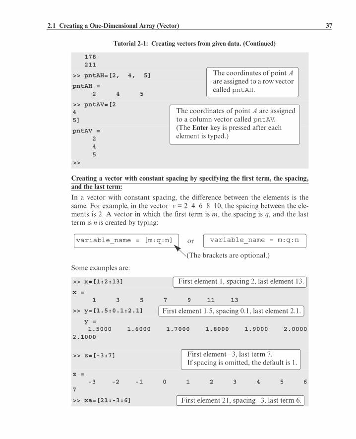
Creating a vector with constant spacing by specifying the first term, the spacing,and the last term:
In a vector with constant spacing, the difference between the elements is thesame. For example, in the vector v = 2 4 6 8 10, the spacing between the ele-ments is 2. A vector in which the first term is m, the spacing is q, and the lastterm is n is created by typing:
Some examples are:
178 211
>> pntAH=[2, 4, 5]
pntAH = 2 4 5
>> pntAV=[245]
pntAV = 2 4 5>>
>> x=[1:2:13]
x = 1 3 5 7 9 11 13
>> y=[1.5:0.1:2.1]
y = 1.5000 1.6000 1.7000 1.8000 1.9000 2.00002.1000
>> z=[-3:7]
z = -3 -2 -1 0 1 2 3 4 5 67
>> xa=[21:-3:6]
Tutorial 2-1: Creating vectors from given data. (Continued)
The coordinates of point A are assigned to a row vector called pntAH.
The coordinates of point A are assignedto a column vector called pntAV.(The Enter key is pressed after eachelement is typed.)
variable_name = [m:q:n] variable_name = m:q:nor
(The brackets are optional.)
First element 1, spacing 2, last element 13.
First element 1.5, spacing 0.1, last element 2.1.
First element –3, last term 7.If spacing is omitted, the default is 1.
First element 21, spacing –3, last term 6.

38 Chapter 2: Creating Arrays
• If the numbers m, q, and n are such that the value of n cannot be obtained byadding q’s to m, then (for positive n) the last element in the vector will be the lastnumber that does not exceed n.
• If only two numbers (the first and the last terms) are typed (the spacing is omit-ted), then the default for the spacing is 1.
Creating a vector with linear (equal) spacing by specifying the first and last terms,and the number of terms:
A vector with n elements that are linearly (equally) spaced in which the first ele-ment is xi and the last element is xf can be created by typing the linspacecommand (MATLAB determines the correct spacing):
When the number of elements is omitted, the default is 100. Some examples are:
xa = 21 18 15 12 9 6>>
>> va=linspace(0,8,6)
va = 0 1.6000 3.2000 4.8000 6.4000 8.0000
>> vb=linspace(30,10,11)
vb = 30 28 26 24 22 20 18 16 14 12 10
>> u=linspace(49.5,0.5)
u = Columns 1 through 10 49.5000 49.0051 48.5101 48.0152 47.5202 47.025346.5303 46.0354 45.5404 45.0455............Columns 91 through 100 4.9545 4.4596 3.9646 3.4697 2.9747 2.47981.9848 1.4899 0.9949 0.5000>>
variable_name = linspace(xi,xf,n)
First element
Last element
Number ofelements
6 elements, first element 0, last element 8.
11 elements, first element 30, last element 10.
When the number of elements isomitted, the default is 100.
First element 49.5, last element 0.5.
100 elements are displayed.

2.2 Creating a Two-Dimensional Array (Matrix) 39
2.2 CREATING A TWO-DIMENSIONAL ARRAY (MATRIX)
A two-dimensional array, also called a matrix, has numbers in rows and col-umns. Matrices can be used to store information like the arrangement in a table.Matrices play an important role in linear algebra and are used in science andengineering to describe many physical quantities.
In a square matrix the number of rows and the number of columns is equal.For example, the matrix
7 4 93 8 1 matrix6 5 3
is square, with three rows and three columns. In general, the number of rowsand columns can be different. For example, the matrix:
31 26 14 18 5 30 3 51 20 11 43 65 matrix28 6 15 61 34 2214 58 6 36 93 7
has four rows and six columns. A matrix has m rows and n columns, andm by n is called the size of the matrix.
A matrix is created by assigning the elements of the matrix to a variable.This is done by typing the elements, row by row, inside square brackets [ ]. Firsttype the left bracket [ then type the first row, separating the elements withspaces or commas. To type the next row type a semicolon or press Enter. Typethe right bracket ] at the end of the last row.
The elements that are entered can be numbers or mathematical expressions thatmay include numbers, predefined variables, and functions. All the rows musthave the same number of elements. If an element is zero, it has to be entered assuch. MATLAB displays an error message if an attempt is made to define anincomplete matrix. Examples of matrices defined in different ways are shown inTutorial 2-2.
Tutorial 2-2: Creating matrices.
>> a=[5 35 43; 4 76 81; 21 32 40]
a = 5 35 43 4 76 81 21 32 40
>> b = [7 2 76 33 81 98 6 25 65 54 68 9 0]
variable_name=[1st row elements; 2nd row elements; 3rd row elements; ... ; last row elements]
A semicolon is typed beforea new line is entered.
The Enter key is pressedbefore a new line is entered.

40 Chapter 2: Creating Arrays
Rows of a matrix can also be entered as vectors using the notation for creat-ing vectors with constant spacing, or the linspace command. For example:
In this example the first two rows were entered as vectors using the notation ofconstant spacing, the third row was entered using the linspace command,and in the last row the elements were entered individually.
2.2.1 The zeros, ones and, eye Commands
The zeros(m,n), ones(m,n), and eye(n) commands can be used to creatematrices that have elements with special values. The zeros(m,n) and theones(m,n) commands create a matrix with m rows and n columns in which allelements are the numbers 0 and 1, respectively. The eye(n) command creates asquare matrix with n rows and n columns in which the diagonal elements areequal to 1 and the rest of the elements are 0. This matrix is called the identitymatrix. Examples are:
b = 7 2 76 33 8 1 98 6 25 6 5 54 68 9 0
>> cd=6; e=3; h=4;
>> Mat=[e, cd*h, cos(pi/3); h^2, sqrt(h*h/cd), 14]
Mat = 3.0000 24.0000 0.5000 16.0000 1.6330 14.0000>>
>> A=[1:2:11; 0:5:25; linspace(10,60,6); 67 2 43 68 4 13]
A = 1 3 5 7 9 11 0 5 10 15 20 25 10 20 30 40 50 60 67 2 43 68 4 13>>
>> zr=zeros(3,4)
zr = 0 0 0 0 0 0 0 0 0 0 0 0
>> ne=ones(4,3)
Tutorial 2-2: Creating matrices. (Continued)
Three variables are defined.
Elements are defined by mathematical expressions.

2.3 Notes About Variables in MATLAB 41
Matrices can also be created as a result of mathematical operations withvectors and matrices. This topic is covered in Chapter 3.
2.3 NOTES ABOUT VARIABLES IN MATLAB
• All variables in MATLAB are arrays. A scalar is an array with one element, avector is an array with one row or one column of elements, and a matrix is anarray with elements in rows and columns.
• The variable (scalar, vector, or matrix) is defined by the input when the variableis assigned. There is no need to define the size of the array (single element for ascalar, a row or a column of elements for a vector, or a two-dimensional array ofelements for a matrix) before the elements are assigned.
• Once a variable exists—as a scalar, vector, or matrix—it can be changed to anyother size, or type, of variable. For example, a scalar can be changed to a vectoror a matrix; a vector can be changed to a scalar, a vector of different length, or amatrix; and a matrix can be changed to have a different size, or be reduced to avector or a scalar. These changes are made by adding or deleting elements. Thissubject is covered in Sections 2.7 and 2.8.
2.4 THE TRANSPOSE OPERATOR
The transpose operator, when applied to a vector, switches a row (column) vec-tor to a column (row) vector. When applied to a matrix, it switches the rows(columns) to columns (rows). The transpose operator is applied by typing a sin-gle quote ’ following the variable to be transposed. Examples are:
ne = 1 1 1 1 1 1 1 1 1 1 1 1
>> idn=eye(5)
idn = 1 0 0 0 0 0 1 0 0 0 0 0 1 0 0 0 0 0 1 0 0 0 0 0 1>>
>> aa=[3 8 1]
aa = 3 8 1
>> bb=aa'
Define a row vector aa.
Define a column vector bb as the transpose of vector aa.

42 Chapter 2: Creating Arrays
2.5 ARRAY ADDRESSING
Elements in an array (either vector or matrix) can be addressed individually orin subgroups. This is useful when there is a need to redefine only some of the ele-ments, when specific elements are to be used in calculations, or when a subgroupof the elements is used to define a new variable.
2.5.1 Vector
The address of an element in a vector is its position in the row (or column). Fora vector named ve, ve(k) refers to the element in position k. The first positionis 1. For example, if the vector ve has nine elements:
ve = 35 46 78 23 5 14 81 3 55
then
ve(4) = 23, ve(7) = 81, and ve(1) = 35.
A single vector element, v(k), can be used just as a variable. For example, itis possible to change the value of only one element of a vector by assigning anew value to a specific address. This is done by typing: v(k) = value. A single ele-ment can also be used as a variable in a mathematical expression. Examples are:
bb = 3 8 1
>> C=[2 55 14 8; 21 5 32 11; 41 64 9 1]
C = 2 55 14 8 21 5 32 11 41 64 9 1
>> D=C'
D = 2 21 41 55 5 64 14 32 9 8 11 1>>
>> VCT=[35 46 78 23 5 14 81 3 55]
VCT = 35 46 78 23 5 14 81 3 55
>> VCT(4)
Define a matrix C with 3 rows and 4 columns.
Define a matrix D as the transpose of matrix C. (D has 4 rows and 3 columns.)
Define a vector.
Display the fourth element.

2.5 Array Addressing 43
2.5.2 Matrix
The address of an element in a matrix is its position, defined by the row numberand the column number where it is located. For a matrix assigned to a variablema, ma(k,p) refers to the element in row k and column p.
For example, if the matrix is:
then ma(1,1) = 3 and ma(2,3) = 10.
As with vectors, it is possible to change the value of just one element of amatrix by assigning a new value to that element. Also, single elements can beused like variables in mathematical expressions and functions. Some examplesare:
ans = 23
>> VCT(6)=273
VCT = 35 46 78 23 5 273 81 3 55
>> VCT(2)+VCT(8)ans = 49
>> VCT(5)^VCT(8)+sqrt(VCT(7))
ans = 134>>
>> MAT=[3 11 6 5; 4 7 10 2; 13 9 0 8]
MAT = 3 11 6 5 4 7 10 2 13 9 0 8
>> MAT(3,1)=20
MAT = 3 11 6 5 4 7 10 2 20 9 0 8
>> MAT(2,4)-MAT(1,2)
ans = -9
Assign a new value to the sixth element.
The whole vector is displayed.
Use the vector elements in mathematical expressions.
Create a matrix.
Assign a new value to the (3,1) element.
Use elements in a mathematical expression.
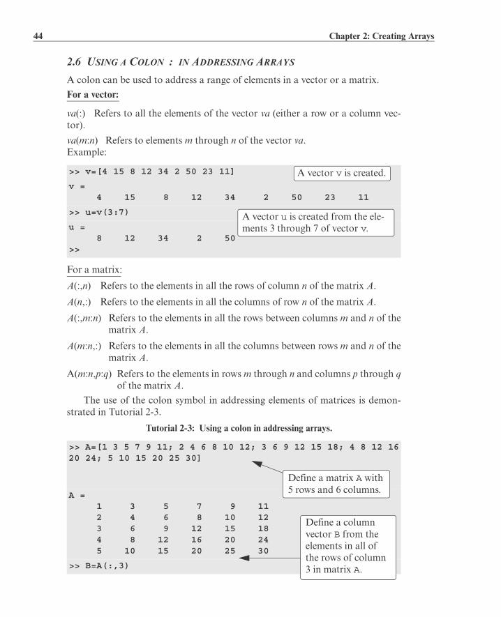
44 Chapter 2: Creating Arrays
2.6 USING A COLON : IN ADDRESSING ARRAYS
A colon can be used to address a range of elements in a vector or a matrix.
For a vector:
va(:) Refers to all the elements of the vector va (either a row or a column vec-tor).
va(m:n) Refers to elements m through n of the vector va.Example:
For a matrix:
A(:,n) Refers to the elements in all the rows of column n of the matrix A.
A(n,:) Refers to the elements in all the columns of row n of the matrix A.
A(:,m:n) Refers to the elements in all the rows between columns m and n of thematrix A.
A(m:n,:) Refers to the elements in all the columns between rows m and n of thematrix A.
A(m:n,p:q) Refers to the elements in rows m through n and columns p through qof the matrix A.
The use of the colon symbol in addressing elements of matrices is demon-strated in Tutorial 2-3.
>> v=[4 15 8 12 34 2 50 23 11]
v = 4 15 8 12 34 2 50 23 11
>> u=v(3:7)
u = 8 12 34 2 50>>
Tutorial 2-3: Using a colon in addressing arrays.
>> A=[1 3 5 7 9 11; 2 4 6 8 10 12; 3 6 9 12 15 18; 4 8 12 1620 24; 5 10 15 20 25 30]
A = 1 3 5 7 9 11 2 4 6 8 10 12 3 6 9 12 15 18 4 8 12 16 20 24 5 10 15 20 25 30
>> B=A(:,3)
A vector v is created.
A vector u is created from the ele-ments 3 through 7 of vector v.
Define a matrix A with5 rows and 6 columns.
Define a column vector B from the elements in all of the rows of column 3 in matrix A.

2.6 Using a Colon : in Addressing Arrays 45
In Tutorial 2-3 new vectors and matrices are created from existing ones byusing a range of elements, or a range of rows and columns (using :). It is possi-ble, however, to select only specific elements, or specific rows and columns ofexisting variables to create new variables. This is done by typing the selected ele-ments or rows or columns inside brackets, as shown below:
B = 5 6 9 12 15
>> C=A(2,:)
C = 2 4 6 8 10 12
>> E=A(2:4,:)
E = 2 4 6 8 10 12 3 6 9 12 15 18 4 8 12 16 20 24
>> F=A(1:3,2:4)
F = 3 5 7 4 6 8 6 9 12>>
>> v=4:3:34
v = 4 7 10 13 16 19 22 25 28 31 34
>> u=v([3, 5, 7:10])
u = 10 16 22 25 28 31
>> A=[10:-1:4; ones(1,7); 2:2:14; zeros(1,7)]
A = 10 9 8 7 6 5 4 1 1 1 1 1 1 1 2 4 6 8 10 12 14 0 0 0 0 0 0 0
>> B = A([1,3],[1,3,5:7])
Tutorial 2-3: Using a colon in addressing arrays. (Continued)
Define a row vector C from the elements in all of the columns of row 2 in matrix A.
Define a matrix E from the ele-ments in rows 2 through 4 and all the columns in matrix A.
Create a matrix F from the ele-ments in rows 1 through 3 and col-umns 2 through 4 in matrix A.
Create a vector v with 11 elements.
Create a vector u from the 3rd, the 5th, and the 7th through 10th elements of v.
Create a matrix A.
Create a matrix B from the 1st and 3rd rows, and 1st, 3rd, and the 5th through 7th columns of A.
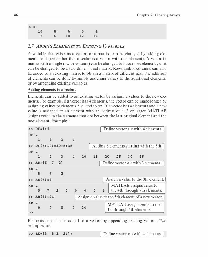
46 Chapter 2: Creating Arrays
2.7 ADDING ELEMENTS TO EXISTING VARIABLES
A variable that exists as a vector, or a matrix, can be changed by adding ele-ments to it (remember that a scalar is a vector with one element). A vector (amatrix with a single row or column) can be changed to have more elements, or itcan be changed to be a two-dimensional matrix. Rows and/or columns can alsobe added to an existing matrix to obtain a matrix of different size. The additionof elements can be done by simply assigning values to the additional elements,or by appending existing variables.
Adding elements to a vector:
Elements can be added to an existing vector by assigning values to the new ele-ments. For example, if a vector has 4 elements, the vector can be made longer byassigning values to elements 5, 6, and so on. If a vector has n elements and a newvalue is assigned to an element with an address of n+2 or larger, MATLABassigns zeros to the elements that are between the last original element and thenew element. Examples:
Elements can also be added to a vector by appending existing vectors. Twoexamples are:
B = 10 8 6 5 4 2 6 10 12 14
>> DF=1:4
DF = 1 2 3 4
>> DF(5:10)=10:5:35
DF = 1 2 3 4 10 15 20 25 30 35
>> AD=[5 7 2]
AD = 5 7 2
>> AD(8)=4
AD = 5 7 2 0 0 0 0 4
>> AR(5)=24
AR = 0 0 0 0 24>>
>> RE=[3 8 1 24];
Define vector DF with 4 elements.
Adding 6 elements starting with the 5th.
Define vector AD with 3 elements.
Assign a value to the 8th element.
MATLAB assigns zeros to the 4th through 7th elements.
Assign a value to the 5th element of a new vector.
MATLAB assigns zeros to the 1st through 4th elements.
Define vector RE with 4 elements.

2.7 Adding Elements to Existing Variables 47
Adding elements to a matrix:Rows and/or columns can be added to an existing matrix by assigning values tothe new rows or columns. This can be done by assigning new values, or byappending existing variables. This must be done carefully since the size of theadded rows or columns must fit the existing matrix. Examples are:
>> GT=4:3:16;
>> KNH=[RE GT]
KNH = 3 8 1 24 4 7 10 13 16
>> KNV=[RE'; GT']
KNV = 3 8 1 24 4 7 10 13 16
>> E=[1 2 3 4; 5 6 7 8]
E = 1 2 3 4 5 6 7 8
>> E(3,:)=[10:4:22]
E = 1 2 3 4 5 6 7 8 10 14 18 22
>> K=eye(3)
K = 1 0 0 0 1 0 0 0 1
>> G=[E K]
G = 1 2 3 4 1 0 0 5 6 7 8 0 1 0 10 14 18 22 0 0 1
Define vector GT with 5 elements.
Define a new vector KNH by appending RE and GT.
Create a new column vector KNVby appending RE’ and GT’.
Define a matrix E.
Add the vector 10 14 18 22 as the third row of E.
Define a matrix K.
Append matrix K to matrix E. The num-bers of rows in E and K must be the same.

48 Chapter 2: Creating Arrays
If a matrix has a size of and a new value is assigned to an elementwith an address beyond the size of the matrix, MATLAB increases the size ofthe matrix to include the new element. Zeros are assigned to the other elementsthat are added. Examples:
2.8 DELETING ELEMENTS
An element, or a range of elements, of an existing variable can be deleted by re-assigning nothing to these elements. This is done by using square brackets withnothing typed in between them. By deleting elements, a vector can be madeshorter and a matrix can be made smaller. Examples are:
>> AW=[3 6 9; 8 5 11]
AW = 3 6 9 8 5 11
>> AW(4,5)=17
AW = 3 6 9 0 0 8 5 11 0 0 0 0 0 0 0 0 0 0 0 17
>> BG(3,4)=15
BG = 0 0 0 0 0 0 0 0 0 0 0 15>>
>> kt=[2 8 40 65 3 55 23 15 75 80]
kt = 2 8 40 65 3 55 23 15 75 80
>> kt(6)=[]
kt = 2 8 40 65 3 23 15 75 80
>> kt(3:6)=[]
kt = 2 8 15 75 80
>> mtr=[5 78 4 24 9; 4 0 36 60 12; 56 13 5 89 3]
Define a matrix.
Assign a value to the (4,5) element.
MATLAB changes the matrix size to , and assigns zeros to the new elements.
Assign a value to the (3,4) element of a new matrix.
MATLAB creates a matrixand assigns zeros to all the ele-ments except BG(3,4).
Define a vector with 10 elements.
Eliminate the 6th element.
The vector now has 9 elements.
Eliminate elements 3 through 6.
The vector now has 5 elements.
Define a matrix.
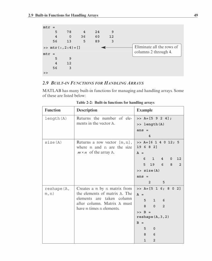
2.9 Built-in Functions for Handling Arrays 49
2.9 BUILT-IN FUNCTIONS FOR HANDLING ARRAYS
MATLAB has many built-in functions for managing and handling arrays. Someof these are listed below:
mtr = 5 78 4 24 9 4 0 36 60 12 56 13 5 89 3
>> mtr(:,2:4)=[]
mtr = 5 9 4 12 56 3>>
Table 2-2: Built-in functions for handling arrays
Function Description Example
length(A) Returns the number of ele-ments in the vector A.
>> A=[5 9 2 4];
>> length(A)
ans =
4
size(A) Returns a row vector [m,n],where m and n are the size
of the array A.
>> A=[6 1 4 0 12; 5 19 6 8 2]
A =
6 1 4 0 12
5 19 6 8 2
>> size(A)
ans =
2 5
reshape(A,m,n)
Creates a m by n matrix fromthe elements of matrix A. Theelements are taken columnafter column. Matrix A musthave m times n elements.
>> A=[5 1 6; 8 0 2]
A =
5 1 6
8 0 2
>> B = reshape(A,3,2)
B =
5 0
8 6
1 2
Eliminate all the rows of columns 2 through 4.

50 Chapter 2: Creating Arrays
Additional built-in functions for manipulation of arrays are described in theHelp Window. In this window, select “MATLAB,” then in the Contents “Func-tions,” and then “By Category.”
Sample Problem 2-1: Create a matrix
Using the ones and zeros commands, create a matrix in which the first tworows are 0s and the next two rows are 1s.
Solution
diag(v) When v is a vector, creates asquare matrix with the ele-ments of v in the diagonal.
>> v=[7 4 2];
>> A=diag(v)
A =
7 0 0
0 4 0
0 0 2
diag(A) When A is a matrix, creates avector from the diagonal ele-ments of A.
>> A=[1 2 3; 4 5 6; 7 8 9]
A =
1 2 3
4 5 6
7 8 9
>> vec=diag(A)
vec =
1
5
9
>> A(1:2,:)=zeros(2,5)
A = 0 0 0 0 0 0 0 0 0 0
>> A(3:4,:)=ones(2,5)
A = 0 0 0 0 0 0 0 0 0 0 1 1 1 1 1 1 1 1 1 1
Table 2-2: Built-in functions for handling arrays (Continued)
Function Description Example
First, create a matrix with 0s.
Add rows 3 and 4 with 1s.

2.9 Built-in Functions for Handling Arrays 51
A different solution to the problem is:
Sample Problem 2-2: Create a matrix
Create a matrix in which the middle two rows and the middle two columnsare 1s and the rest of the entries are 0s.
Solution
>> A=[zeros(2,5);ones(2,5)]
A = 0 0 0 0 0 0 0 0 0 0 1 1 1 1 1 1 1 1 1 1
>> AR=zeros(6,6)
AR = 0 0 0 0 0 0 0 0 0 0 0 0 0 0 0 0 0 0 0 0 0 0 0 0 0 0 0 0 0 0 0 0 0 0 0 0
>> AR(3:4,:)=ones(2,6)
AR = 0 0 0 0 0 0 0 0 0 0 0 0 1 1 1 1 1 1 1 1 1 1 1 1 0 0 0 0 0 0 0 0 0 0 0 0
>> AR(:,3:4)=ones(6,2)
AR = 0 0 1 1 0 0 0 0 1 1 0 0 1 1 1 1 1 1 1 1 1 1 1 1 0 0 1 1 0 0 0 0 1 1 0 0
Create a matrix from two matrices.
First, create a matrix with 0s.
Reassign the number 1 to the 3rd and 4th rows.
Reassign the num-ber 1 to the 3rd and 4th columns.
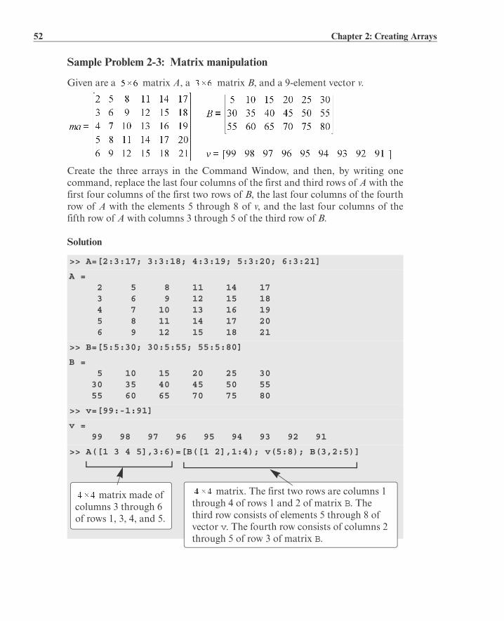
52 Chapter 2: Creating Arrays
Sample Problem 2-3: Matrix manipulation
Given are a matrix A, a matrix B, and a 9-element vector v.
Create the three arrays in the Command Window, and then, by writing onecommand, replace the last four columns of the first and third rows of A with thefirst four columns of the first two rows of B, the last four columns of the fourthrow of A with the elements 5 through 8 of v, and the last four columns of thefifth row of A with columns 3 through 5 of the third row of B.
Solution
>> A=[2:3:17; 3:3:18; 4:3:19; 5:3:20; 6:3:21]
A = 2 5 8 11 14 17 3 6 9 12 15 18 4 7 10 13 16 19 5 8 11 14 17 20 6 9 12 15 18 21
>> B=[5:5:30; 30:5:55; 55:5:80]
B = 5 10 15 20 25 30 30 35 40 45 50 55 55 60 65 70 75 80
>> v=[99:-1:91]
v = 99 98 97 96 95 94 93 92 91
>> A([1 3 4 5],3:6)=[B([1 2],1:4); v(5:8); B(3,2:5)]
matrix. The first two rows are columns 1 through 4 of rows 1 and 2 of matrix B. The third row consists of elements 5 through 8 of vector v. The fourth row consists of columns 2 through 5 of row 3 of matrix B.
matrix made of columns 3 through 6 of rows 1, 3, 4, and 5.

2.10 Strings and Strings as Variables 53
2.10 STRINGS AND STRINGS AS VARIABLES
• A string is an array of characters. It is created by typing the characters withinsingle quotes.
• Strings can include letters, digits, other symbols, and spaces.
• Examples of strings: 'ad ef ', '3%fr2', '{edcba:21!', 'MATLAB'.
• A string that contains a single quote is created by typing two single quoteswithin the string.
• When a string is being typed in, the color of the text on the screen changes tomaroon when the first single quote is typed. When the single quote at the end ofthe string is typed, the color of the string changes to purple.
Strings have several different uses in MATLAB. They are used in outputcommands to display text messages (Chapter 4), in formatting commands ofplots (Chapter 5), and as input arguments of some functions (Chapter 7). Moredetails are given in these chapters when strings are used for these purposes.• When strings are being used in formatting plots (labels to axes, title, and text
notes), characters within the string can be formatted to have a specified font,size, position (uppercase, lowercase), color, etc. See Chapter 5 for details.
Strings can also be assigned to variables by simply typing the string on theright side of the assignment operator, as shown in the examples below:
When a variable is defined as a string, the characters of the string are storedin an array just as numbers are. Each character, including a space, is an elementin the array. This means that a one-line string is a row vector in which the num-ber of elements is equal to the number of characters. The elements of the vectorsare addressed by position. For example, in the vector B that was defined above
A = 2 5 5 10 15 20 3 6 9 12 15 18 4 7 30 35 40 45 5 8 95 94 93 92 6 9 60 65 70 75
>> a='FRty 8'
a =FRty 8
>> B='My name is John Smith'
B =My name is John Smith>>
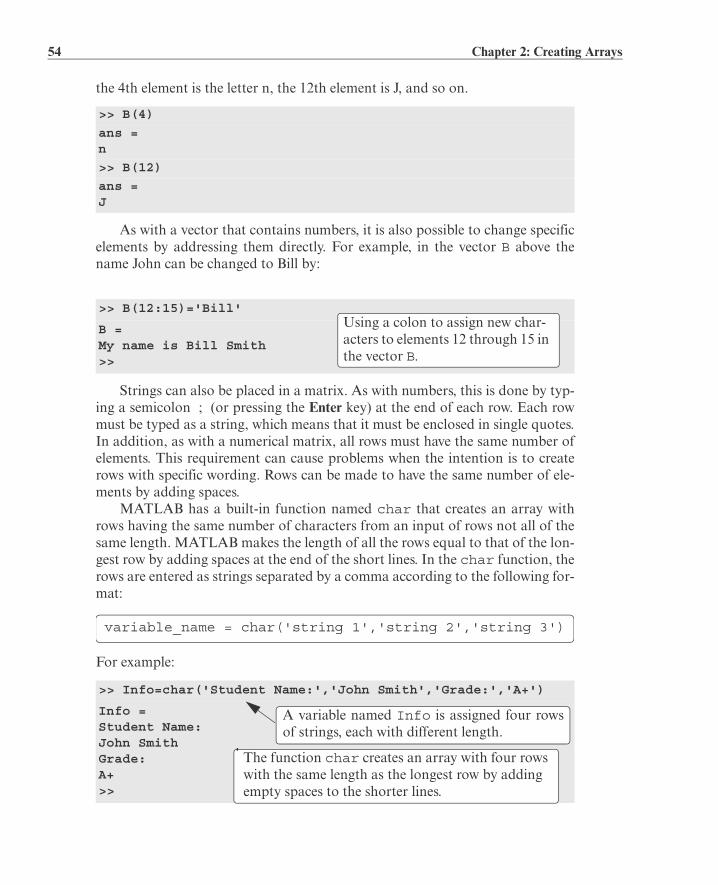
54 Chapter 2: Creating Arrays
the 4th element is the letter n, the 12th element is J, and so on.
As with a vector that contains numbers, it is also possible to change specificelements by addressing them directly. For example, in the vector B above thename John can be changed to Bill by:
Strings can also be placed in a matrix. As with numbers, this is done by typ-ing a semicolon ; (or pressing the Enter key) at the end of each row. Each rowmust be typed as a string, which means that it must be enclosed in single quotes.In addition, as with a numerical matrix, all rows must have the same number ofelements. This requirement can cause problems when the intention is to createrows with specific wording. Rows can be made to have the same number of ele-ments by adding spaces.
MATLAB has a built-in function named char that creates an array withrows having the same number of characters from an input of rows not all of thesame length. MATLAB makes the length of all the rows equal to that of the lon-gest row by adding spaces at the end of the short lines. In the char function, therows are entered as strings separated by a comma according to the following for-mat:
For example:
>> B(4)
ans =n
>> B(12)
ans =J
>> B(12:15)='Bill'
B =My name is Bill Smith>>
>> Info=char('Student Name:','John Smith','Grade:','A+')
Info =Student Name:John Smith Grade: A+>>
Using a colon to assign new char-acters to elements 12 through 15 in the vector B.
variable_name = char('string 1','string 2','string 3')
A variable named Info is assigned four rowsof strings, each with different length.
The function char creates an array with four rows with the same length as the longest row by adding empty spaces to the shorter lines.
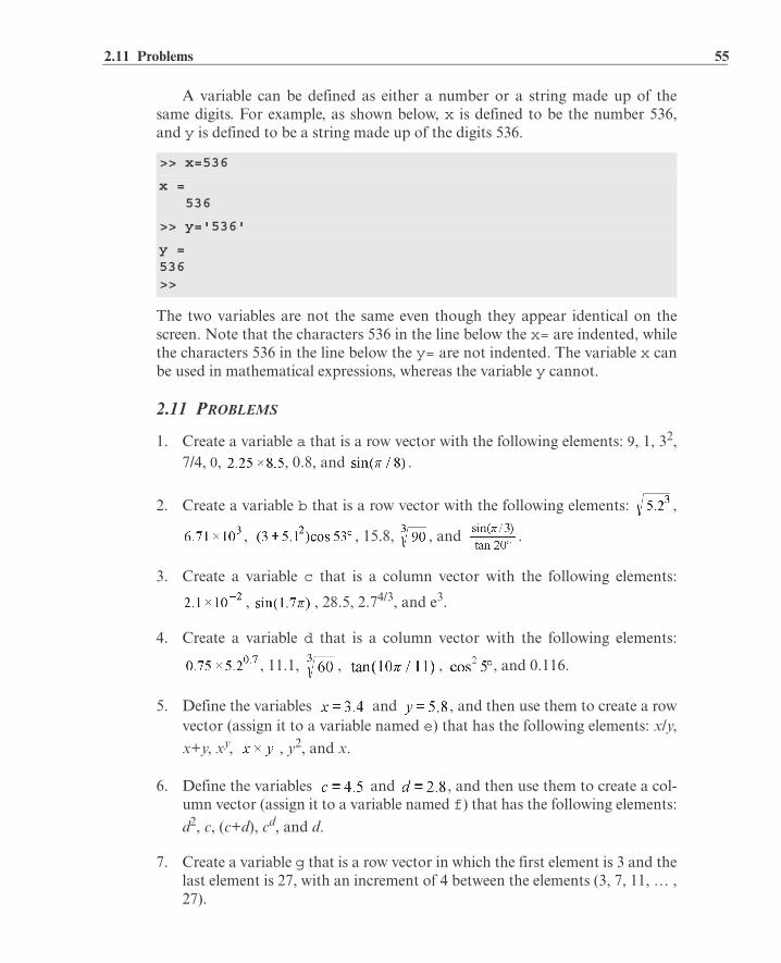
2.11 Problems 55
A variable can be defined as either a number or a string made up of thesame digits. For example, as shown below, x is defined to be the number 536,and y is defined to be a string made up of the digits 536.
The two variables are not the same even though they appear identical on thescreen. Note that the characters 536 in the line below the x= are indented, whilethe characters 536 in the line below the y= are not indented. The variable x canbe used in mathematical expressions, whereas the variable y cannot.
2.11 PROBLEMS
1. Create a variable a that is a row vector with the following elements: 9, 1, 32,7/4, 0, , 0.8, and .
2. Create a variable b that is a row vector with the following elements: ,
, , 15.8, , and .
3. Create a variable c that is a column vector with the following elements:
, , 28.5, 2.74/3, and e3.
4. Create a variable d that is a column vector with the following elements:
, 11.1, , , , and 0.116.
5. Define the variables and , and then use them to create a rowvector (assign it to a variable named e) that has the following elements: x/y,
x+y, xy, , y2, and x.
6. Define the variables and , and then use them to create a col-umn vector (assign it to a variable named f) that has the following elements:
d2, c, (c+d), cd, and d.
7. Create a variable g that is a row vector in which the first element is 3 and thelast element is 27, with an increment of 4 between the elements (3, 7, 11, … ,27).
>> x=536
x = 536
>> y='536'
y =536>>
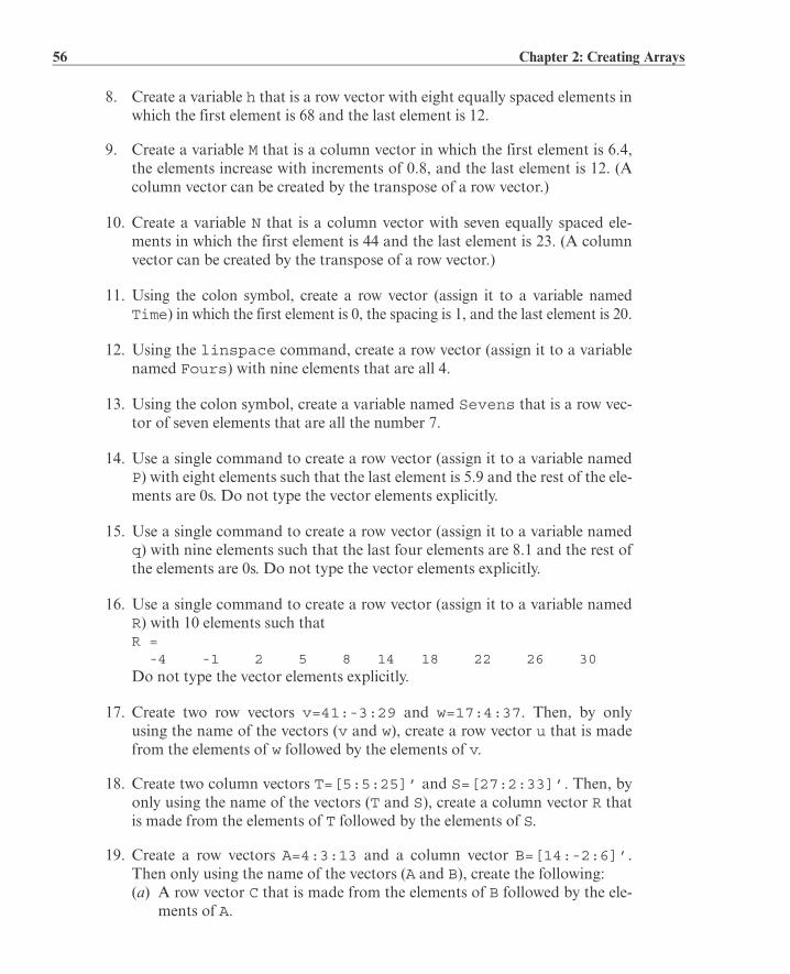
56 Chapter 2: Creating Arrays
8. Create a variable h that is a row vector with eight equally spaced elements inwhich the first element is 68 and the last element is 12.
9. Create a variable M that is a column vector in which the first element is 6.4,the elements increase with increments of 0.8, and the last element is 12. (Acolumn vector can be created by the transpose of a row vector.)
10. Create a variable N that is a column vector with seven equally spaced ele-ments in which the first element is 44 and the last element is 23. (A columnvector can be created by the transpose of a row vector.)
11. Using the colon symbol, create a row vector (assign it to a variable namedTime) in which the first element is 0, the spacing is 1, and the last element is 20.
12. Using the linspace command, create a row vector (assign it to a variablenamed Fours) with nine elements that are all 4.
13. Using the colon symbol, create a variable named Sevens that is a row vec-tor of seven elements that are all the number 7.
14. Use a single command to create a row vector (assign it to a variable namedP) with eight elements such that the last element is 5.9 and the rest of the ele-ments are 0s. Do not type the vector elements explicitly.
15. Use a single command to create a row vector (assign it to a variable namedq) with nine elements such that the last four elements are 8.1 and the rest ofthe elements are 0s. Do not type the vector elements explicitly.
16. Use a single command to create a row vector (assign it to a variable namedR) with 10 elements such thatR =
-4 -1 2 5 8 14 18 22 26 30 Do not type the vector elements explicitly.
17. Create two row vectors v=41:-3:29 and w=17:4:37. Then, by onlyusing the name of the vectors (v and w), create a row vector u that is madefrom the elements of w followed by the elements of v.
18. Create two column vectors T=[5:5:25]’ and S=[27:2:33]’. Then, byonly using the name of the vectors (T and S), create a column vector R thatis made from the elements of T followed by the elements of S.
19. Create a row vectors A=4:3:13 and a column vector B=[14:-2:6]’.Then only using the name of the vectors (A and B), create the following:(a) A row vector C that is made from the elements of B followed by the ele-
ments of A.
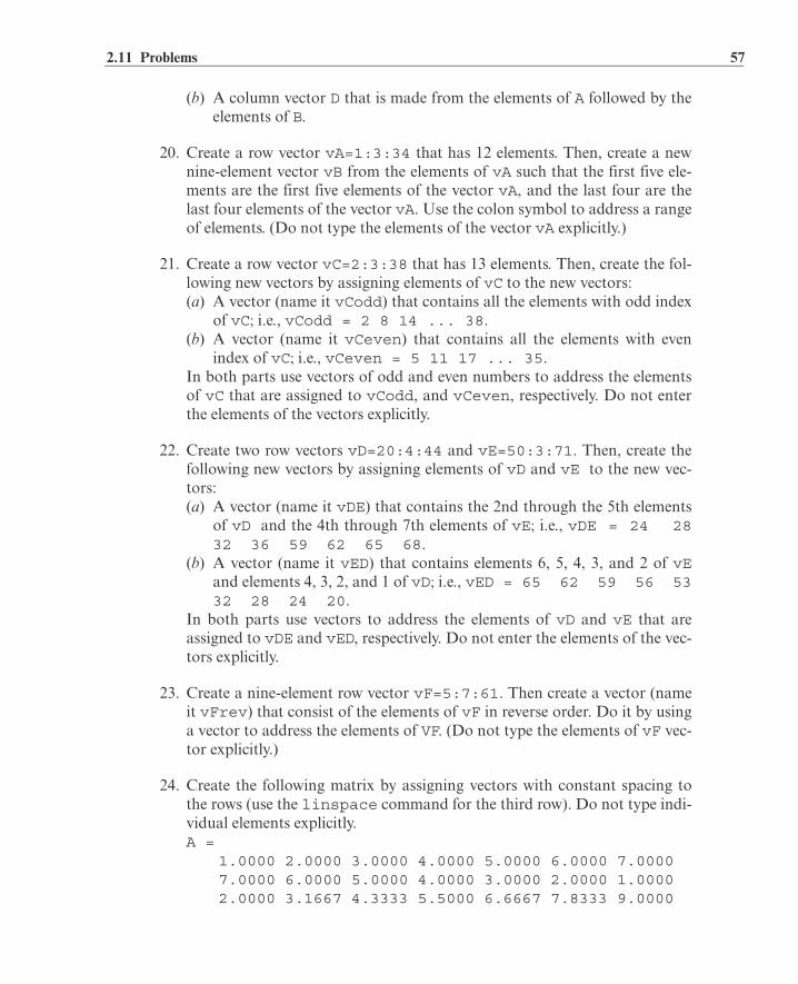
2.11 Problems 57
(b) A column vector D that is made from the elements of A followed by theelements of B.
20. Create a row vector vA=1:3:34 that has 12 elements. Then, create a newnine-element vector vB from the elements of vA such that the first five ele-ments are the first five elements of the vector vA, and the last four are thelast four elements of the vector vA. Use the colon symbol to address a rangeof elements. (Do not type the elements of the vector vA explicitly.)
21. Create a row vector vC=2:3:38 that has 13 elements. Then, create the fol-
lowing new vectors by assigning elements of vC to the new vectors:(a) A vector (name it vCodd) that contains all the elements with odd index
of vC; i.e., vCodd = 2 8 14 ... 38.(b) A vector (name it vCeven) that contains all the elements with even
index of vC; i.e., vCeven = 5 11 17 ... 35.In both parts use vectors of odd and even numbers to address the elementsof vC that are assigned to vCodd, and vCeven, respectively. Do not enterthe elements of the vectors explicitly.
22. Create two row vectors vD=20:4:44 and vE=50:3:71. Then, create thefollowing new vectors by assigning elements of vD and vE to the new vec-tors:(a) A vector (name it vDE) that contains the 2nd through the 5th elements
of vD and the 4th through 7th elements of vE; i.e., vDE = 24 2832 36 59 62 65 68.
(b) A vector (name it vED) that contains elements 6, 5, 4, 3, and 2 of vEand elements 4, 3, 2, and 1 of vD; i.e., vED = 65 62 59 56 5332 28 24 20.
In both parts use vectors to address the elements of vD and vE that areassigned to vDE and vED, respectively. Do not enter the elements of the vec-tors explicitly.
23. Create a nine-element row vector vF=5:7:61. Then create a vector (nameit vFrev) that consist of the elements of vF in reverse order. Do it by usinga vector to address the elements of VF. (Do not type the elements of vF vec-tor explicitly.)
24. Create the following matrix by assigning vectors with constant spacing tothe rows (use the linspace command for the third row). Do not type indi-vidual elements explicitly.A = 1.0000 2.0000 3.0000 4.0000 5.0000 6.0000 7.0000 7.0000 6.0000 5.0000 4.0000 3.0000 2.0000 1.0000 2.0000 3.1667 4.3333 5.5000 6.6667 7.8333 9.0000

58 Chapter 2: Creating Arrays
25. Create the following vector by using the linspace command. Do not typeindividual elements explicitly.B = 4 4 4 4 4 5 5 5 5
26. Create the following matrix by typing one command. Do not type individ-ual elements explicitly.C =
6 8 6 8 6 8 6 8 6 8
27. Create the following matrix by typing one command. Do not type individ-ual elements explicitly.D =
1 1 1 1 1 1 1 1 1 1 1 1 8 6 4 2
28. Create the following matrix by typing one command. Do not type individ-ual elements explicitly.E =
0 0 0 0 8 0 0 0 0 7 0 0 0 0 6
29. Create the following matrix by typing one command. Do not type individ-ual elements explicitly.F =
0 0 0 0 0 0 0 0 0 0 0 0 0 0 8 6 4 2
30. Create the following matrix by typing one command. Do not type individ-ual elements explicitly.G =
1 1 1 1 1 1 1 1 1 1 1 1 1 1 1 0 0 0 1 1 0 0 0 1 1 0 0 0 1 1
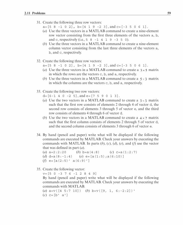
2.11 Problems 59
31. Create the following three row vectors:a=[5 8 -1 0 2], b=[4 1 9 -2 3], and c=[-3 5 0 6 1]. (a) Use the three vectors in a MATLAB command to create a nine-element
row vector consisting from the first three elements of the vectors a, b,and c, respectively (i.e., 5 8 -1 4 1 9 -3 5 0).
(b) Use the three vectors in a MATLAB command to create a nine-elementcolumn vector consisting from the last three elements of the vectors a,b, and c, respectively.
32. Create the following three row vectors:a=[5 8 -1 0 2], b=[4 1 9 -2 3], and c=[-3 5 0 6 1]. (a) Use the three vectors in a MATLAB command to create a matrix
in which the rows are the vectors c, b, and a, respectively.(b) Use the three vectors in a MATLAB command to create a matrix
in which the columns are the vectors c, b, and a, respectively.
33. Create the following two row vectors:d=[6-1 4 0 -2 5], and e=[7 5 9 0 1 3].(a) Use the two vectors in a MATLAB command to create a matrix
such that the first row consists of elements 2 through 4 of vector d, thesecond row consists of elements 3 through 5 of vector e, and the thirdrow consists of elements 4 through 6 of vector d.
(b) Use the two vectors in a MATLAB command to create a matrixsuch that the first column consists of elements 2 through 5 of vector d,and the second column consists of elements 3 through 6 of vector e.
34. By hand (pencil and paper) write what will be displayed if the followingcommands are executed by MATLAB. Check your answers by executing thecommands with MATLAB. In parts (b), (c), (d), (e), and (f) use the vectorthat was defined in part (a).(a) a=2:2:20 (b) b=a(4:8) (c) c=a(1:2:7)(d) d=a(8:-1:4) (e) e=[a(1:5);a(6:10)](f) e=[a(2:5)’ a(6:9)’]
35. Create the following vector:v=[5 0 -3 7 6 -1 2 8 4 9]By hand (pencil and paper) write what will be displayed if the followingcommands are executed by MATLAB. Check your answers by executing thecommands with MATLAB.(a) a=v([4 5:7 10]) (b) b=v([9, 1, 6:-2:2])' (c) c=[b' a']

60 Chapter 2: Creating Arrays
36. Create the following vectors:u=[0 9 -5 6 3 -1 2] and w=[-2 3 7 -4 0 1 5]By hand (pencil and paper) write what will be displayed if the followingcommands are executed by MATLAB. Check your answers by executing thecommands with MATLAB.(a) A=[u(2:5);w([7 5]) u([6 7])](b) B=[w(4:7)', zeros(4,2), u([1 3 5 7])']
37. Create the following matrix M: M =
1 7 13 19 25 3 9 15 21 27 5 11 17 23 29
By writing one command and using the colon to address range of elements(do not type individual elements explicitly), use the matrix M to:(a) Create a five-element row vector named Va that contains the elements
of the third row of M.(b) Create a three-element column vector named Vb that contains the ele-
ments of the fourth column of M.(c) Create an eight-element row vector named Vc that contains the ele-
ments of the second row of M followed by the elements of the third col-umn of M.
38. Create the following matrix N:N =
0 3 6 9 12 15 18 21 24 27 30 33 36 39 42 45 48 51
(It can be done by typing: N=reshape(0:3:51,6,3)'.) By writing one command and using the colon to address range of elements(do not type individual elements explicitly), use the matrix N to:
(a) Create a six-element row vector named Ua that contains the first threeelements of the first row of N followed by the last three elements of thethird row of N.
(b) Create a nine-element column vector named Ub that contains the ele-ments of the first column of N, followed by the elements of the third col-umn of N, followed by the elements of the sixth column of N.
(c) Create a six-element column vector named Uc that contains elements 2, 3,4, and 5 of the second row of N, followed by elements 2 and 3 of the fifthcolumn of N.

2.11 Problems 61
39. Create the following matrix G: G = 0.1 0.2 0.3 0.4 0.5 0.6 0.7 10 9 8 7 6 5 4 0 0.2 0.4 0.6 0.8 1.0 1.2 5 3 1 -1 -3 -5 -7
(a) Create a matrix Ma from the first, third, and fourth rows and thefirst two and last two columns of matrix G.
(b) Create a matrix Mb from the first three rows and the second,fourth, and sixth columns of matrix G.
40. Create the following matrix K: K = 0.25 0.5 0.75 1.0 1.25 1.5 1.75 2 4 6 8 10 12 14 25 30 35 40 45 50 55
(a) Create a matrix Ga such that its first row includes the elements ofthe second column of K followed by the elements of the fifth column ofK, the second row of Ga includes the first six elements of the second rowof K, and the third row of Ga includes the last six elements of the thirdrow of K.
(b) Create a matrix Gb from the first two rows and columns 3 through6 of K.
41. The following matrix is defined in MATLAB:S = 1 2 3 4 5 6 7 8 9 10 11 12 13 14 15 16 17 18 19 20 21 22 23 24
By hand (pencil and paper) write what will be displayed if the followingcommands are executed by MATLAB. Check your answers by executing thecommands with MATLAB.(a) A=S(2,[2,4]) (b) B=S(3,[3:5])(c) C=S([2:4],[4:6]) (d) D=S(:,[1:3])
42. The following matrix is defined in MATLAB: T = 2 4 6 8 10 12 14 16 18 20 22 24 26 28 30

62 Chapter 2: Creating Arrays
By hand (pencil and paper) write what will be displayed if the followingcommands are executed by MATLAB. Check your answers by executing thecommands with MATLAB.(a) D=[T(1,1:4);T(3,2:5)](b) E=[T(:,4); T(2,:)'](c) F(3:5,3:5)=T(1:3,1:3)
43. By hand (pencil and paper) write what will be displayed if the followingcommands are executed by MATLAB. Check your answers by executing thecommands with MATLAB.V=[1:2:11;13:2:23]V(:,4:6)=V(:,1:3)V(3:4,:)=VV(:,[2:3 5:6])=[]
44. Using the zeros, ones, and eye commands, create the following arrays bytyping one command:
(a) (b) (c)
45. Use the eye, ones, and zeros commands to create the following arrays:
Using the variables A, B, and C, write a command that creates the followingmatrix D:

63
Chapter 3 Mathematical Operations with Arrays
Once variables are created in MATLAB they can be used in a wide variety ofmathematical operations. In Chapter 1 the variables that were used in mathe-matical operations were all defined as scalars. This means that they were all
arrays (arrays with one row and one column that have only one element)and the mathematical operations were done with single numbers. Arrays, how-ever, can be one-dimensional (arrays with one row, or with one column), two-dimensional (arrays with multiple rows and columns), and even of higherdimensions. In these cases the mathematical operations are more complex.MATLAB, as its name indicates, is designed to carry out advanced array opera-tions that have many applications in science and engineering. This chapter pres-ents the basic, most common mathematical operations that MATLAB performsusing arrays.
Addition and subtraction are relatively simple operations and are coveredfirst, in Section 3.1. The other basic operations—multiplication, division, andexponentiation—can be done in MATLAB in two different ways. One way,which uses the standard symbols (*, /, and ^), follows the rules of linear algebraand is presented in Sections 3.2 and 3.3. The second way, which is called ele-ment-by-element operations, is covered in Section 3.4. These operations use thesymbols .*, ./, and .^ (a period is typed in front of the standard operation sym-bol). In addition, in both types of calculations, MATLAB has left division oper-ators ( .\ or \ ), which are also explained in Sections 3.3 and 3.4.
A Note to First-Time Users of MATLAB:
Although matrix operations are presented first and element-by-element opera-tions next, the order can be reversed since the two are independent of eachother. It is expected that almost every MATLAB user has some knowledge ofmatrix operations and linear algebra, and thus will be able to follow the materialcovered in Sections 3.2 and 3.3 without any difficulty. Some readers, however,might prefer to read Section 3.4 first. MATLAB can be used with element-by-element operations in numerous applications that do not require linear algebramultiplication (or division) operations.

64 Chapter 3: Mathematical Operations with Arrays
3.1 ADDITION AND SUBTRACTION
The operations + (addition) and – (subtraction) can be used to add (subtract)arrays of identical size (the same numbers of rows and columns) and to add(subtract) a scalar to an array. When two arrays are involved the sum, or the dif-ference, of the arrays is obtained by adding, or subtracting, their correspondingelements.
In general, if A and B are two arrays (for example, matrices),
and
then the matrix that is obtained by adding A and B is:
Examples are:
>> VectA=[8 5 4]; VectB=[10 2 7];
>> VectC=VectA+VectB
VectC = 18 7 11
>> A=[5 -3 8; 9 2 10]
A = 5 -3 8 9 2 10
>> B=[10 7 4; -11 15 1]
B = 10 7 4 -11 15 1
>> A-B
ans = -5 -10 4 20 -13 9
>> C=A+B
C = 15 4 12 -2 17 11
>> VectA+A
??? Error using ==> plusMatrix dimensions must agree. >>
Define two vectors.
Define a vector VectC that is equal to VectA+VectB.
Define two matrices A and B.
Subtracting matrix B from matrix A.
Define a matrix C that is equal to A+B.
Trying to add arrays of different size.
An error message is displayed.

3.2 Array Multiplication 65
When a scalar (number) is added to (or subtracted from) an array, the scalaris added to (or subtracted from) all the elements of the array. Examples are:
3.2 ARRAY MULTIPLICATION
The multiplication operation * is executed by MATLAB according to the rulesof linear algebra. This means that if A and B are two matrices, the operationA*B can be carried out only if the number of columns in matrix A is equal to thenumber of rows in matrix B. The result is a matrix that has the same number ofrows as A and the same number of columns as B. For example, if A is a matrix and B is a matrix:
and
then the matrix that is obtained with the operation A*B has dimensions with the elements:
A numerical example is:
>> VectA=[1 5 8 -10 2]VectA = 1 5 8 -10 2
>> VectA+4
ans = 5 9 12 -6 6
>> A=[6 21 -15; 0 -4 8]
A = 6 21 -15 0 -4 8
>> A-5ans = 1 16 -20 -5 -9 3
Define a vector named VectA.
Add the scalar 4 to VectA.
4 is added to each element of VectA.
Define a matrix A.
Subtract the scalar 5 from A.
5 is subtracted from each element of A.

66 Chapter 3: Mathematical Operations with Arrays
The product of the multiplication of two square matrices (they must be ofthe same size) is a square matrix of the same size. However, the multiplication ofmatrices is not commutative. This means that if A and B are both , then
. Also, the power operation can be executed only with a squarematrix (since A*A can be carried out only if the number of columns in the firstmatrix is equal to the number of rows in the second matrix).
Two vectors can be multiplied only if they have the same number of ele-ments, and one is a row vector and the other is a column vector. The multiplica-tion of a row vector by a column vector gives a matrix, which is a scalar.This is the dot product of two vectors. (MATLAB also has a built-in function,dot(a,b), that computes the dot product of two vectors.) When using the dotfunction, the vectors a and b can each be a row vector or a column vector (seeTable 3-1). The multiplication of a column vector by a row vector, each with nelements, gives an matrix Multiplication of array is demonstrated in Tuto-rial 3-1.
Tutorial 3-1: Multiplication of arrays.
>> A=[1 4 2; 5 7 3; 9 1 6; 4 2 8]
A = 1 4 2 5 7 3 9 1 6 4 2 8
>> B=[6 1; 2 5; 7 3]
B = 6 1 2 5 7 3
>> C=A*B
C = 28 27 65 49 98 32 84 38
>> D=B*A??? Error using ==> *Inner matrix dimensions must agree.
>> F=[1 3; 5 7]
F = 1 3 5 7
>> G=[4 2; 1 6]
Define a matrix A.
Define a matrix B.
Multiply matrix A by matrix B and assign the result to variable C.
Trying to multiply B by A, B*A, gives an error since the number of columns in B is 2 and the number of rows in A is 4.
Define two matrices F and G.

3.2 Array Multiplication 67
When an array is multiplied by a number (actually a number is a array),each element in the array is multiplied by the number. For example:
G = 4 2 1 6
>> F*G
ans = 7 20 27 52
>> G*F
ans = 14 26 31 45
>> AV=[2 5 1]
AV = 2 5 1
>> BV=[3; 1; 4]
BV = 3 1 4
>> AV*BV
ans = 15
>> BV*AV
ans = 6 15 3 2 5 1 8 20 4>>
>> A=[2 5 7 0; 10 1 3 4; 6 2 11 5]
A = 2 5 7 0 10 1 3 4 6 2 11 5
>> b=3
b = 3
Tutorial 3-1: Multiplication of arrays. (Continued)
Multiply F*G
Multiply G*F
Note that the answer for G*F is not thesame as the answer for F*G.
Define a three-element row vector AV.
Define a three-element column vector BV.
Multiply AV by BV. The answer is a scalar. (Dot product of two vectors.)
Multiply BV by AV. The answer is a matrix.
Define a matrix A.
Assign the number 3 to the variable b.

68 Chapter 3: Mathematical Operations with Arrays
Linear algebra rules of array multiplication provide a convenient way forwriting a system of linear equations. For example, the system of three equationswith three unknowns
can be written in a matrix form as:
and in matrix notation as
AX = B where , , and .
3.3 ARRAY DIVISION
The division operation is also associated with the rules of linear algebra. Thisoperation is more complex, and only a brief explanation is given below. A fullexplanation can be found in books on linear algebra.
The division operation can be explained with the help of the identity matrixand the inverse operation.
Identity matrix:
The identity matrix is a square matrix in which the diagonal elements are 1s andthe rest of the elements are 0s. As was shown in Section 2.2.1, an identity matrixcan be created in MATLAB with the eye command. When the identity matrixmultiplies another matrix (or vector), that matrix (or vector) is unchanged (the
>> b*A
ans = 6 15 21 0 30 3 9 12 18 6 33 15
>> C=A*5
C = 10 25 35 0 50 5 15 20 30 10 55 25
Multiply the matrix A by b. This can bedone by either typing b*A or A*b.
Multiply the matrix A by 5 and assign the result to a new variable C. (Typing C=5*A gives the same result.)

3.3 Array Division 69
multiplication has to be done according to the rules of linear algebra). This isequivalent to multiplying a scalar by 1. For example:
or or
If a matrix A is square, it can be multiplied by the identity matrix, I, from the leftor from the right:
AI = IA = A
Inverse of a matrix:
The matrix B is the inverse of the matrix A if, when the two matrices are multi-plied, the product is the identity matrix. Both matrices must be square, and themultiplication order can be BA or AB.
BA = AB = I
Obviously B is the inverse of A, and A is the inverse of B. For example:
The inverse of a matrix A is typically written as A-1. In MATLAB the inverse ofa matrix can be obtained either by raising A to the power of –1, A^-1, or withthe inv(A) function. Multiplying the matrices above with MATLAB is shownbelow.
>> A=[2 1 4; 4 1 8; 2 -1 3]
A = 2 1 4 4 1 8 2 -1 3
>> B=inv(A)
B = 5.5000 -3.5000 2.0000 2.0000 -1.0000 0 -3.0000 2.0000 -1.0000
>> A*B
ans = 1 0 0 0 1 0 0 0 1
Creating the matrix A.
Use the inv function to find theinverse of A and assign it to B.
Multiplication of A and B gives the identity matrix.

70 Chapter 3: Mathematical Operations with Arrays
Not every matrix has an inverse. A matrix has an inverse only if it is square andits determinant is not equal to zero.
Determinants:
A determinant is a function associated with square matrices. A short review ondeterminants is given below. For a more detailed coverage refer to books on lin-ear algebra.
The determinant is a function that associates with each square matrix A anumber, called the determinant of the matrix. The determinant is typicallydenoted by det(A) or |A|. The determinant is calculated according to specificrules. For a second-order matrix, the rule is:
, for example,
The determinant of a square matrix can be calculated with the det command (see Table 3-1).
Array division:
MATLAB has two types of array division, right division and left division.
Left division, \ :
Left division is used to solve the matrix equation . In this equation Xand B are column vectors. This equation can be solved by multiplying, on theleft, both sides by the inverse of A:
The left-hand side of this equation is X, since
So the solution of is:
In MATLAB the last equation can be written by using the left division charac-ter:
X = A\BIt should be pointed out here that although the last two operations appear togive the same result, the method by which MATLAB calculates X is different. In
the first, MATLAB calculates and then uses it to multiply B. In the second(left division), the solution X is obtained numerically using a method that isbased on Gauss elimination. The left division method is recommended for solv-
>> A*A^-1
ans = 1 0 0 0 1 0 0 0 1
Use the power –1 to find the inverse of A.Multiplying it by A gives the identity matrix.

3.3 Array Division 71
ing a set of linear equations, because the calculation of the inverse may be lessaccurate than the Gauss elimination method when large matrices are involved.
Right division, / :
The right division is used to solve the matrix equation . In this equationX and D are row vectors. This equation can be solved by multiplying, on theright, both sides by the inverse of C:
which gives
In MATLAB the last equation can be written using the right division character:
X = D/C
The following example demonstrates the use of the left and right division,and the inv function to solve a set of linear equations.
Sample Problem 3-1: Solving three linear equations (array division)
Use matrix operations to solve the following system of linear equations.
Solution
Using the rules of linear algebra demonstrated earlier, the above system of equa-tions can be written in the matrix form AX=B or in the form XC=D:
or
Solutions for both forms are shown below:
>> A=[4 -2 6; 2 8 2; 6 10 3];
>> B=[8; 4; 0];
>> X=A\BX = -1.8049 0.2927 2.6341
>> Xb=inv(A)*B
Xb = -1.8049 0.2927 2.6341
Solving the form AX = B.
Solving by using left division: X = A \ B.
Solving by using the inverse of A: X=A-1B.

72 Chapter 3: Mathematical Operations with Arrays
3.4 ELEMENT-BY-ELEMENT OPERATIONS
In Sections 3.2 and 3.3 it was shown that when the regular symbols for multipli-cation and division (* and /) are used with arrays, the mathematical operationsfollow the rules of linear algebra. There are, however, many situations thatrequire element-by-element operations. These operations are carried out oneach of the elements of the array (or arrays). Addition and subtraction are bydefinition already element-by-element operations, since when two arrays areadded (or subtracted) the operation is executed with the elements that are in thesame position in the arrays. Element-by-element operations can be done onlywith arrays of the same size.
Element-by-element multiplication, division, or exponentiation of two vec-tors or matrices is entered in MATLAB by typing a period in front of the arith-metic operator.
If two vectors a and b are a=[a1 a2 a3 a4] and b=[b1 b2 b3 b4], then element-by-element multiplication, division, and exponentiation of the two vectors gives:
>> C=[4 2 6; -2 8 10; 6 2 3];
>> D=[8 4 0];
>> Xc=D/C
Xc = -1.8049 0.2927 2.6341
>> Xd=D*inv(C)
Xd = -1.8049 0.2927 2.6341
Symbol Description Symbol Description
.* Multiplication ./ Right division
.^ Exponentiation .\ Left Division
Solving the form XC = D.
Solving by using right division: X = D/C.
Solving by using the inverse of C: X=DC-1.

3.4 Element-by-Element Operations 73
If two matrices A and B are
and
then element-by-element multiplication and division of the two matrices give:
A .* B = A ./ B =
Element-by-element exponentiation of matrix A gives:
A .^ n =
Element-by-element multiplication, division, and exponentiation aredemonstrated in Tutorial 3-2.
Tutorial 3-2: Element-by-element operations.
>> A=[2 6 3; 5 8 4]
A = 2 6 3 5 8 4
>> B=[1 4 10; 3 2 7]
B = 1 4 10 3 2 7
>> A.*B
ans = 2 24 30 15 16 28
>> C=A./B
C = 2.0000 1.5000 0.3000 1.6667 4.0000 0.5714
A
A11 A12 A13
A21 A22 A23
A31 A32 A33
= B
B11 B12 B13
B21 B22 B23
B31 B32 B33
=
A11B11 A12B12 A13B13
A21B21 A22B22 A23B23
A31B31 A32B32 A33B33
A11 B11 A12 B12 A13 B13
A21 B21 A22 B22 A23 B23
A31 B31 A32 B32 A33 B33
A11n A12
n A13n
A21n A22
n A23n
A31n A32
n A33n
Define a array A.2 3
Define a array B.2 3
Element-by-element multipli-cation of array A by B.
Element-by-element division of array A by B. The result is assigned to variable C.

74 Chapter 3: Mathematical Operations with Arrays
Element-by-element calculations are very useful for calculating the value ofa function at many values of its argument. This is done by first defining a vectorthat contains values of the independent variable, and then using this vector inelement-by-element computations to create a vector in which each element is thecorresponding value of the function. One example is:
In the example above . Element-by-element operation is needed whenx is squared. Each element in the vector y is the value of y that is obtained whenthe value of the corresponding element of the vector x is substituted in the equa-tion. Another example is:
In the last example . Element-by-element operations are used in this
example three times: to calculate z3 and z2, and to divide the numerator by thedenominator.
>> B.^3
ans = 1 64 1000 27 8 343
>> A*B
??? Error using ==> *Inner matrix dimensions must agree.
>> x=[1:8]
x = 1 2 3 4 5 6 7 8
>> y=x.^2-4*x
y = -3 -4 -3 0 5 12 21 32>>
>> z=[1:2:11]
z = 1 3 5 7 9 11
>> y=(z.^3 + 5*z)./(4*z.^2 - 10)
y = -1.0000 1.6154 1.6667 2.0323 2.4650 2.9241
Tutorial 3-2: Element-by-element operations. (Continued)
Element-by-element exponen-tiation of array B. The result is an array in which each term is the corresponding term in B raised to the power of 3.
Trying to multiply A*B gives an error, since A and B cannot be multiplied according to lin-ear algebra rules. (The number of columns in A is not equal to the number of rows in B.)
Create a vector x with eight elements.
Vector x is used in element-by-element calculations of the elements of vector y.
Create a vector z with six elements.
Vector z is used in element-by-element calculations of the elements of vector y.

3.5 Using Arrays in MATLAB Built-in Math Functions 75
3.5 USING ARRAYS IN MATLAB BUILT-IN MATH FUNCTIONS
The built-in functions in MATLAB are written such that when the argument(input) is an array, the operation that is defined by the function is executed oneach element of the array. (One can think of the operation as element-by-ele-ment application of the function.) The result (output) from such an operation isan array in which each element is calculated by entering the corresponding ele-ment of the argument (input) array into the function. For example, if a vectorwith seven elements is substituted in the function cos(x), the result is a vectorwith seven elements in which each element is the cosine of the correspondingelement in x. This is shown below.
An example in which the argument variable is a matrix is:
The feature of MATLAB in which arrays can be used as arguments in functionsis called vectorization.
3.6 BUILT-IN FUNCTIONS FOR ANALYZING ARRAYS
MATLAB has many built-in functions for analyzing arrays. Table 3-1 lists someof these functions.
>> x=[0:pi/6:pi]
x = 0 0.5236 1.0472 1.5708 2.0944 2.6180 3.1416
>>y=cos(x)
y = 1.0000 0.8660 0.5000 0.0000 -0.5000 -0.8660 -1.0000>>
>> d=[1 4 9; 16 25 36; 49 64 81]
d = 1 4 9 16 25 36 49 64 81
>> h=sqrt(d)
h = 1 2 3 4 5 6 7 8 9
Creating a array.
h is a array in which eachelement is the square root of thecorresponding element in array d.

76 Chapter 3: Mathematical Operations with Arrays
Table 3-1: Built-in array functions
Function Description Example
mean(A) If A is a vector, returns the mean value of the elements of the vector.
>> A=[5 9 2 4];>> mean(A)ans = 5
C=max(A)
[d,n]=max(A)
If A is a vector, C is the largest element in A. If A is a matrix, C is a row vector containing the largest ele-ment of each column of A.
If A is a vector, d is the largest element in A, and n is the position of the ele-ment (the first if several have the max value).
>> A=[5 9 2 4 11 6 111];>> C=max(A)C = 11
>> [d,n]=max(A)d = 11n = 5
min(A)
[d,n]=min(A)
The same as max(A), but for the smallest element.
The same as [d,n]= max(A), but for the small-est element.
>> A=[5 9 2 4];>> min(A)ans = 2
sum(A) If A is a vector, returns the sum of the elements of the vector.
>> A=[5 9 2 4];>> sum(A)ans = 20
sort(A) If A is a vector, arranges the elements of the vector in ascending order.
>> A=[5 9 2 4];>> sort(A)ans = 2 4 5 9
median(A) If A is a vector, returns the median value of the ele-ments of the vector.
>> A=[5 9 2 4];>> median(A)ans = 4.5000

3.7 Generation of Random Numbers 77
3.7 GENERATION OF RANDOM NUMBERS
Simulations of many physical processes and engineering applications frequentlyrequire using a number (or a set of numbers) with a random value. MATLABhas three commands—rand, randn, and randi—that can be used to assignrandom numbers to variables.
The rand command:
The rand command generates uniformly distributed random numbers with val-ues between 0 and 1. The command can be used to assign these numbers to ascalar, a vector, or a matrix, as shown in Table 3-2.
std(A) If A is a vector, returns the standard deviation of the elements of the vector.
>> A=[5 9 2 4];>> std(A)ans = 2.9439
det(A) Returns the determinant of a square matrix A.
>> A=[2 4; 3 5];>> det(A)ans = -2
dot(a,b) Calculates the scalar (dot) product of two vectors a and b. The vectors can each be row or column vec-tors.
>> a=[1 2 3];>> b=[3 4 5];>> dot(a,b)ans = 26
cross(a,b) Calculates the cross prod-uct of two vectors a and b, (axb). The two vectors must have each three ele-ments.
>> a=[1 3 2];>> b=[2 4 1];>> cross(a,b)ans = -5 3 -2
inv(A) Returns the inverse of a square matrix A.
>> A=[2 -2 1; 3 2 -1; 2 -3 2];>> inv(A)ans = 0.2000 0.20000 -1.6000 0.40001.0000 -2.6000 0.40002.0000
Table 3-1: Built-in array functions (Continued)
Function Description Example

78 Chapter 3: Mathematical Operations with Arrays
Sometimes there is a need for random numbers that are distributed in aninterval other than (0,1), or for numbers that are integers only. This can be doneusing mathematical operations with the rand function. Random numbers thatare distributed in a range (a,b) can be obtained by multiplying rand by (b – a)and adding the product to a:
(b – a)*rand + a
For example, a vector of 10 elements with random values between –5 and 10 canbe created by (a = –5, b = 10):
The randi command:
The randi command generates uniformly distributed random integer. Thecommand can be used to assign these numbers to a scalar, a vector, or a matrix,as shown in Table 3-3.
Table 3-2: The rand command
Command Description Example
rand Generates a single ran-dom number between 0 and 1.
>> randans = 0.2311
rand(1,n) Generates an n-element row vector of random numbers between 0 and 1.
>> a=rand(1,4)a = 0.6068 0.4860 0.89130.7621
rand(n) Generates an matrix with random numbers between 0 and 1.
>> b=rand(3)b = 0.4565 0.4447 0.9218 0.0185 0.6154 0.7382 0.8214 0.7919 0.1763
rand(m,n) Generates an matrix with random numbers between 0 and 1.
>> c=rand(2,4)c = 0.4057 0.9169 0.89360.3529 0.9355 0.4103 0.05790.8132
rand-perm(n)
Generates a row vector with n elements that are random permutation of integers 1 through n.
>> randperm(8)ans = 8 2 7 4 3 65 1
>> v=15*rand(1,10)-5
v = -1.8640 0.6973 6.7499 5.2127 1.9164 3.51746.9132 -4.1123 4.0430 -4.2460
n n
m n
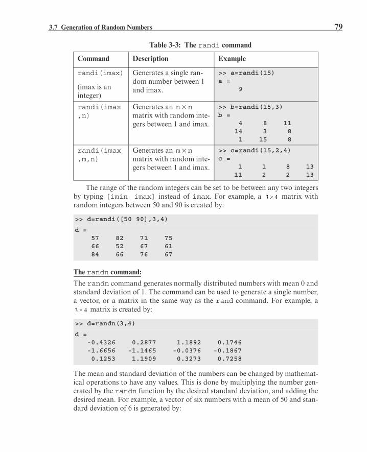
3.7 Generation of Random Numbers 79
The range of the random integers can be set to be between any two integersby typing [imin imax] instead of imax. For example, a matrix withrandom integers between 50 and 90 is created by:
The randn command:
The randn command generates normally distributed numbers with mean 0 andstandard deviation of 1. The command can be used to generate a single number,a vector, or a matrix in the same way as the rand command. For example, a
matrix is created by:
The mean and standard deviation of the numbers can be changed by mathemat-ical operations to have any values. This is done by multiplying the number gen-erated by the randn function by the desired standard deviation, and adding thedesired mean. For example, a vector of six numbers with a mean of 50 and stan-dard deviation of 6 is generated by:
Table 3-3: The randi command
Command Description Example
randi(imax)
(imax is an integer)
Generates a single ran-dom number between 1 and imax.
>> a=randi(15)a = 9
randi(imax,n)
Generates an matrix with random inte-gers between 1 and imax.
>> b=randi(15,3)b = 4 8 11 14 3 8 1 15 8
randi(imax,m,n)
Generates an matrix with random inte-gers between 1 and imax.
>> c=randi(15,2,4)c = 1 1 8 13 11 2 2 13
>> d=randi([50 90],3,4)
d = 57 82 71 75 66 52 67 61 84 66 76 67
>> d=randn(3,4)
d = -0.4326 0.2877 1.1892 0.1746 -1.6656 -1.1465 -0.0376 -0.1867 0.1253 1.1909 0.3273 0.7258
n n
m n

80 Chapter 3: Mathematical Operations with Arrays
Integers of normally distributed numbers can be obtained by using theround function.
3.8 EXAMPLES OF MATLAB APPLICATIONS
Sample Problem 3-2: Equivalent force system (addition of vectors)
Three forces are applied to a bracket asshown. Determine the total (equiva-lent) force applied to the bracket.
Solution
A force is a vector (a physical quantitythat has a magnitude and direction). Ina Cartesian coordinate system a two-dimensional vector F can be written as:
where F is the magnitude of the force and is its angle relative to the x axis, Fx
and Fy are the components of F in the directions of the x and y axes, respec-tively, and i and j are unit vectors in these directions. If Fx and Fy are known,then F and can be determined by:
and
The total (equivalent) force applied on the bracket is obtained by adding theforces that are acting on the bracket. The MATLAB solution below followsthree steps:• Write each force as a vector with two elements, where the first element is the x
component of the vector and the second element is the y component.
• Determine the vector form of the equivalent force by adding the vectors.
• Determine the magnitude and direction of the equivalent force.
The problem is solved in the following program, written in a script file.
>> v=4*randn(1,6)+50
v = 42.7785 57.4344 47.5819 50.4134 52.2527 50.4544
>> w=round(4*randn(1,6)+50)
w = 51 49 46 49 50 44
30o
20o
143o
F2 = 500 NF3 = 700 N
F1 = 400 N
x
y
F Fxi Fyj+ F icos F j F icos jsin+=sin+= =
F Fx2 Fy
2+= tanFy
Fx------=

3.8 Examples of MATLAB Applications 81
When the program is executed, the following is displayed in the Command Win-dow:
The equivalent force has a magnitude of 589.98 N, and is directed (ccw)relative to the x axis. In vector notation, the force is N.
% Sample Problem 3-2 solution (script file)clear
F1M=400; F2M=500; F3M=700;
Th1=-20; Th2=30; Th3=143;
F1=F1M*[cosd(Th1) sind(Th1)]
F2=F2M*[cosd(Th2) sind(Th2)]
F3=F3M*[cosd(Th3) sind(Th3)]
Ftot=F1+F2+F3
FtotM=sqrt(Ftot(1)^2+Ftot(2)^2)
Th=atand(Ftot(2)/Ftot(1))
F1 = 375.8770 -136.8081
F2 = 433.0127 250.0000
F3 = -559.0449 421.2705
Ftot = 249.8449 534.4625
FtotM = 589.9768
Th = 64.9453
Define variables with the magnitude of each vector.
Define variables with the angle of each vector.
Define the three vectors.
Calculate the total force vector.
Calculate the magnitudeof the total force vector.
Calculate the angle of the total force vector.
The components of F1.
The components of F2.
The components of F3.
The components of the total force.
The magnitude of the total force.
The direction of the total force in degrees.
64.95
F 249.84i 534.46j+=

82 Chapter 3: Mathematical Operations with Arrays
Sample Problem 3-3: Friction experiment (element-by-element calculations)
The coefficient of friction, can be determined inan experiment by measuring the force F requiredto move a mass m. When F is measured and m isknown, the coefficient of friction can be calculatedby:
(g = 9.81 m/s2).
Results from measuring F in six tests are given in the table below. Determine thecoefficient of friction in each test, and the average from all tests.
Solution
A solution using MATLAB commands in the Command Window is shownbelow.
Test 1 2 3 4 5 6
Mass m (kg) 2 4 5 10 20 50
Force F (N) 12.5 23.5 30 61 117 294
>> m=[2 4 5 10 20 50];
>> F=[12.5 23.5 30 61 117 294];
>> mu=F./(m*9.81)
mu =
0.6371 0.5989 0.6116 0.6218 0.5963 0.5994
>> mu_ave=mean(mu)
mu_ave = 0.6109
mF
Friction
F mg=
Enter the values of m in a vector.
Enter the values of F in a vector.
A value for mu is calculated for each test, using element-by-element calculations.
The average of the elements in the vector mu is determined by using the function mean.

3.8 Examples of MATLAB Applications 83
Sample Problem 3-4: Electrical resistive network analysis (solving a system of linear equations)
The electrical circuit shown consists ofresistors and voltage sources. Determinethe current in each resistor using the meshcurrent method, which is based on Kirch-hoff’s voltage law.
V, V, V, ,
, , ,
Solution
Kirchhoff’s voltage law states that thesum of the voltage around a closed circuitis zero. In the mesh current method a cur-rent is first assigned for each mesh (i1, i2,i3, i4 in the figure). Then Kirchhoff’s volt-age law is applied for each mesh. Thisresults in a system of linear equations for the currents (in this case four equa-tions). The solution gives the values of the mesh currents. The current in a resis-tor that belongs to two meshes is the sum of the currents in the correspondingmeshes. It is convenient to assume that all the currents are in the same direction(clockwise in this case). In the equation for each mesh, the voltage source is pos-itive if the current flows to the – pole, and the voltage of a resistor is negative forcurrent in the direction of the mesh current.
The equations for the four meshes in the current problem are:
The four equations can be rewritten in matrix form [A][x] = [B]:_
+
+_
+_
i1
i2
i3
i4
R1
R2 R3
R5
R4
R6
R7
R8
V1
V2
V3
V1 20= V2 12= V3 40=R1 18= R2 10= R3 16=R4 6= R5 15= R6 8=R7 12= R8 14=

84 Chapter 3: Mathematical Operations with Arrays
The problem is solved in the following program, written in a script file:
When the script file is executed, the following is displayed in the CommandWindow:
The last column vector gives the current in each mesh. The currents in the resis-tors R1, R5, and R8 are A, A, and A, respec-tively. The other resistors belong to two meshes and their current is the sum ofthe currents in the meshes.The current in resistor R2 is A.The current in resistor R3 is A.The current in resistor R4 is A.The current in resistor R6 is A.The current in resistor R7 is A.
V1=20; V2=12; V3=40;
R1=18; R2=10; R3=16; R4=6;
R5=15; R6=8; R7=12; R8=14;
A=[-(R1+R2+R3) R2 R3 0R2 -(R2+R4+R5+R7) R4 R7R3 R4 -(R3+R4+R6) R60 R7 R6 -(R6+R7+R8)]
>> B=[-V1; 0; V2; -V3]
>> I=A\B
A = -44 10 16 0 10 -43 6 12 16 6 -30 8 0 12 8 -34
B = -20 0 12 -40
I = 0.8411 0.7206 0.6127 1.5750>>
Define variables with the values of the V’s and R’s.
Create the matrix A.
Create the vector B.
Solve for the currents by using left division.
The numerical value of the matrix A.
The numerical value of the vector B.
The solution.i1
i2
i3
i4
i1 0.8411= i2 0.7206= i4 1.5750=
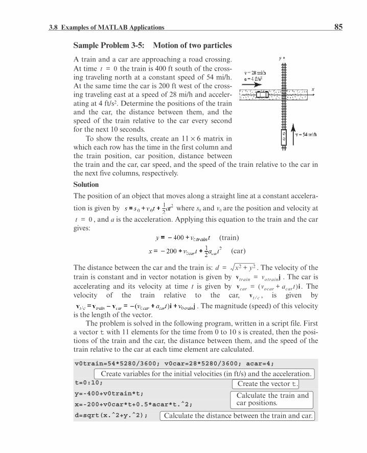
3.8 Examples of MATLAB Applications 85
Sample Problem 3-5: Motion of two particles
A train and a car are approaching a road crossing.At time the train is 400 ft south of the cross-ing traveling north at a constant speed of 54 mi/h.At the same time the car is 200 ft west of the cross-ing traveling east at a speed of 28 mi/h and acceler-ating at 4 ft/s2. Determine the positions of the trainand the car, the distance between them, and thespeed of the train relative to the car every secondfor the next 10 seconds.
To show the results, create an matrix inwhich each row has the time in the first column andthe train position, car position, distance betweenthe train and the car, car speed, and the speed of the train relative to the car inthe next five columns, respectively.
Solution
The position of an object that moves along a straight line at a constant accelera-
tion is given by where s0 and v0 are the position and velocity at
, and a is the acceleration. Applying this equation to the train and the cargives:
(train)
(car)
The distance between the car and the train is: . The velocity of thetrain is constant and in vector notation is given by . The car isaccelerating and its velocity at time t is given by . Thevelocity of the train relative to the car, , is given by
. The magnitude (speed) of this velocityis the length of the vector.
The problem is solved in the following program, written in a script file. Firsta vector t with 11 elements for the time from 0 to 10 s is created, then the posi-tions of the train and the car, the distance between them, and the speed of thetrain relative to the car at each time element are calculated.
v0train=54*5280/3600; v0car=28*5280/3600; acar=4;
t=0:10;
y=-400+v0train*t;
x=-200+v0car*t+0.5*acar*t.^2;
d=sqrt(x.^2+y.^2);
t 0=
11 6
t 0=
d x2 y2+=vtrain votrainj=vcar vocar acart+ i=
vt c
Create variables for the initial velocities (in ft/s) and the acceleration.Create the vector t.
Calculate the train andcar positions.
Calculate the distance between the train and car.

86 Chapter 3: Mathematical Operations with Arrays
Note: In the commands above, table is the name of the variable that is amatrix containing the data to be displayed.
When the script file is executed, the following is displayed in the CommandWindow:
In this problem the results (numbers) are displayed by MATLAB withoutany text. Instructions on how to add text to output generated by MATLAB arepresented in Chapter 4.
3.9 PROBLEMS
Note: Additional problems for practicing mathematical operations with arraysare provided at the end of Chapter 4.
1. For the function , calculate the value of y for the following val-
ues of x using element-by-element operations: .
2. For the function , calculate the value of y for the following values ofx using element-by-element operations: .
vcar=v0car+acar*t;
speed_trainRcar=sqrt(vcar.^2+v0train^2);
table=[t' y' x' d' vcar' speed_trainRcar']
table = 0 -400.0000 -200.0000 447.2136 41.0667 89.2139 1.0000 -320.8000 -156.9333 357.1284 45.0667 91.1243 2.0000 -241.6000 -109.8667 265.4077 49.0667 93.1675 3.0000 -162.4000 -58.8000 172.7171 53.0667 95.3347 4.0000 -83.2000 -3.7333 83.2837 57.0667 97.6178 5.0000 -4.0000 55.3333 55.4777 61.0667 100.0089 6.0000 75.2000 118.4000 140.2626 65.0667 102.5003 7.0000 154.4000 185.4667 241.3239 69.0667 105.0849 8.0000 233.6000 256.5333 346.9558 73.0667 107.7561 9.0000 312.8000 331.6000 455.8535 77.0667 110.5075 10.0000 392.0000 410.6667 567.7245 81.0667 113.3333
Calculate the car’s velocity.
Calculate the speed of the train relative to the car.
Create a table (see note below).
Time(s)
Trainposition(ft)
Carposition(ft)
Car-train distance (ft)
Carspeed(ft/s)
Train speed relative to the car (ft/s)
0 1 2 3 4 5 6 7
1.5 2 2.5 3 3.5 4
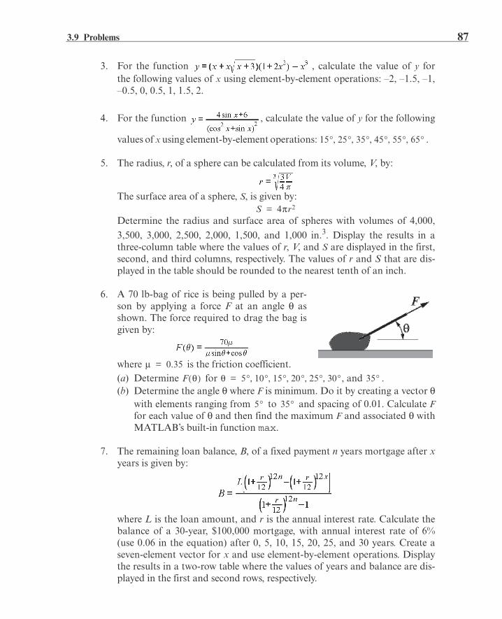
3.9 Problems 87
3. For the function , calculate the value of y forthe following values of x using element-by-element operations: –2, –1.5, –1,–0.5, 0, 0.5, 1, 1.5, 2.
4. For the function , calculate the value of y for the following
values of x using element-by-element operations: .
5. The radius, r, of a sphere can be calculated from its volume, V, by:
The surface area of a sphere, S, is given by:
Determine the radius and surface area of spheres with volumes of 4,000,
3,500, 3,000, 2,500, 2,000, 1,500, and 1,000 in.3. Display the results in athree-column table where the values of r, V, and S are displayed in the first,second, and third columns, respectively. The values of r and S that are dis-played in the table should be rounded to the nearest tenth of an inch.
6. A 70 lb-bag of rice is being pulled by a per-son by applying a force F at an angle asshown. The force required to drag the bag isgiven by:
where is the friction coefficient.(a) Determine for , and . (b) Determine the angle where F is minimum. Do it by creating a vector
with elements ranging from to and spacing of 0.01. Calculate Ffor each value of and then find the maximum F and associated withMATLAB’s built-in function max.
7. The remaining loan balance, B, of a fixed payment n years mortgage after xyears is given by:
where L is the loan amount, and r is the annual interest rate. Calculate thebalance of a 30-year, $100,000 mortgage, with annual interest rate of 6%(use 0.06 in the equation) after 0, 5, 10, 15, 20, 25, and 30 years. Create aseven-element vector for x and use element-by-element operations. Displaythe results in a two-row table where the values of years and balance are dis-played in the first and second rows, respectively.
15 25 35 45 55 65
S 4 r2=
0.35=
F 5 10 15 20 25 30= 35
5 35
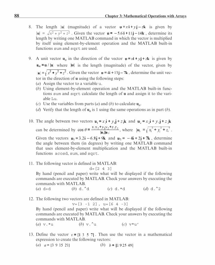
88 Chapter 3: Mathematical Operations with Arrays
8. The length (magnitude) of a vector is given by
. Given the vector , determine itslength by writing one MATLAB command in which the vector is multipliedby itself using element-by-element operation and the MATLAB built-infunctions sum and sqrt are used.
9. A unit vector un in the direction of the vector is given by
where is the length (magnitude) of the vector, given by
. Given the vector , determine the unit vec-tor in the direction of u using the following steps:(a) Assign the vector to a variable u. (b) Using element-by-element operation and the MATLAB built-in func-
tions sum and sqrt calculate the length of u and assign it to the vari-able Lu.
(c) Use the variables from parts (a) and (b) to calculate un.(d) Verify that the length of un is 1 using the same operations as in part (b).
10. The angle between two vectors and
can be determined by , where .
Given the vectors and , determinethe angle between them (in degrees) by writing one MATLAB commandthat uses element-by-element multiplication and the MATLAB built-infunctions acosd, sum, and sqrt.
11. The following vector is defined in MATLAB: d=[2 4 3]
By hand (pencil and paper) write what will be displayed if the followingcommands are executed by MATLAB. Check your answers by executing thecommands with MATLAB.(a) d+d (b) d.^d (c) d.*d (d) d.^2
12. The following two vectors are defined in MATLAB:v=[3 -1 2] , u=[6 4 -3]
By hand (pencil and paper) write what will be displayed if the followingcommands are executed by MATLAB. Check your answers by executing thecommands with MATLAB.(a) v.*u (b) v.^u (c) v*u’
13. Define the vector . Then use the vector in a mathematicalexpression to create the following vectors:(a) (b)
u
u x2 y2 z2+ +=

3.9 Problems 89
(c) (d)
14. Define the vector . Then use the vector in a mathematicalexpression to create the following vectors:
(a) (b)
(c) (d)
15. Define x and y as the vectors and. Then use them in the following expressions to
calculate z using element-by-element calculations.
(a) (b)
16. Define r and s as scalars and , and, t, x, and y as vectors, , and . Then
use these variables to calculate the following expressions using element-by-element calculations for the vectors.
(a) (b)
17. The area of a triangle ABC can be calculatedby , where rAB and rAC are vec-tors connecting the vertices A and B, and Aand C, respectively. Determine the area of thetriangle shown in the figure. Use the follow-ing steps in a script file to calculate the area.First, define the vectors rOA, rOB, and rOC
from knowing the coordinates of points A, B,and C. Then determine the vectors rAB andrAC from rOA, rOB, and rOC. Finally, determine the area by using MATLAB’sbuilt-in functions cross, sum, and sqrt.
18. The cross product of two vectors can be used fordetermining the angle between two vectors:
Use MATLAB’s built-in functions asind,cross, sqrt, and dot to find the angle (indegrees) between and
. Recall that .
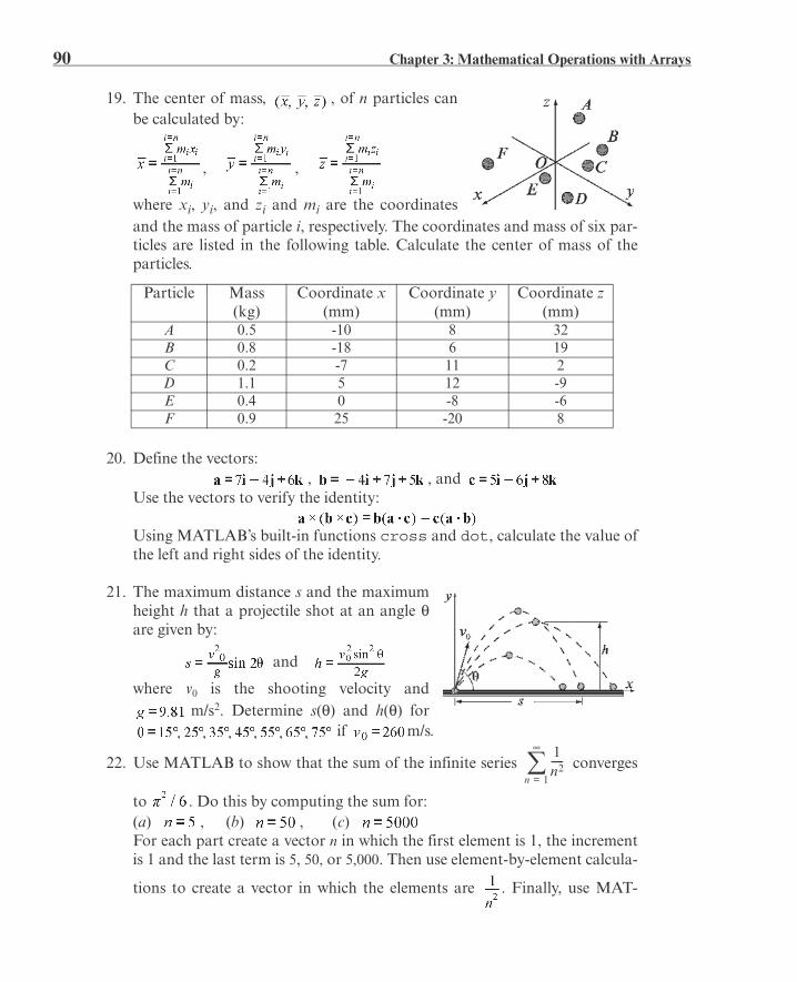
90 Chapter 3: Mathematical Operations with Arrays
19. The center of mass, , of n particles canbe calculated by:
, ,
where xi, yi, and zi and mi are the coordinatesand the mass of particle i, respectively. The coordinates and mass of six par-ticles are listed in the following table. Calculate the center of mass of theparticles.
20. Define the vectors:, , and
Use the vectors to verify the identity:
Using MATLAB’s built-in functions cross and dot, calculate the value ofthe left and right sides of the identity.
21. The maximum distance s and the maximumheight h that a projectile shot at an angle are given by:
and
where v0 is the shooting velocity andm/s2. Determine s( ) and h( ) for
if m/s.
22. Use MATLAB to show that the sum of the infinite series converges
to . Do this by computing the sum for:(a) , (b) , (c)For each part create a vector n in which the first element is 1, the incrementis 1 and the last term is 5, 50, or 5,000. Then use element-by-element calcula-
tions to create a vector in which the elements are . Finally, use MAT-
Particle Mass (kg)
Coordinate x(mm)
Coordinate y(mm)
Coordinate z(mm)
A 0.5 -10 8 32B 0.8 -18 6 19C 0.2 -7 11 2D 1.1 5 12 -9E 0.4 0 -8 -6F 0.9 25 -20 8
1n2-----
n 1=

3.9 Problems 91
LAB’s built-in function sum to sum the series. Compare the values to .Use format long to display the numbers.
23. Use MATLAB to show that the sum of the infinite series converges
to 6. Do this by computing the sum for(a) , (b) , (c) For each part, create a vector n in which the first element is 1, the incrementis 1 and the last term is 5, 15, or 30. Then use element-by-element calcula-
tions to create a vector in which the elements are . Finally, use MAT-
LAB’s built-in function sum to sum the series. Use format long to displaythe numbers.
24. The natural exponential function can be expressed by . Deter-
mine e2 by calculating the sum of the series for:(a) n = 5, (b) n = 15, (c) n = 25
For each part create a vector n in which the first element is 0, the incrementis 1, and the last term is 5, 15, or 25. Then use element-by-element calcula-
tions to create a vector in which the elements are . Finally, use the MAT-
LAB built-in function sum to add the terms of the series. Compare the
values obtained in parts (a), (b), and (c) with the value of e2 calculated byMATLAB.
25. Show that . Do this by first creating a vector x that
has the elements , , , ,
, and . Then, create a new vector y in which each ele-
ment is determined from the elements of x by . Compare the ele-
ments of y with the value . Use format long to display the numbers.
26. Show that . Do this by first creating a vector x that has
the elements 1.0, 0.1, 0.01, 0.001, and 0.0001. Then, create a new vector y in
which each element is determined from the elements of x by .
Compare the elements of y with the value 7.5. Use format long to displaythe numbers.
n 1=
n 0=

92 Chapter 3: Mathematical Operations with Arrays
27. The Hazen Williams equation can be used to calculate the pressure drop, Pd(psi/ft of pipe) in pipes due to friction:
where Q is the flow rate (gpm), C is a design coefficient determined by thetype of pipe, and d is pipe diameter in inches. Consider a 3.5-in.-diametersteel pipe with . Calculate the pressure drop in a 1000-ft-long pipefor flow rates of 250, 300, 350, 400, and 450 gpm. To carry out the calcula-tion, first create a five-element vector with the values of the flow rates (250,300, ...). Then use the vector in the formula using element-by-element oper-ations.
28. The monthly lease payment, Pmt, of a new car can be calculated by:
where Pv and Fv are the present value and the future value (at the end of thelease) of the car, respectively. N is the duration of the lease in months, and iis the interest rate per year. Consider a 36-months-lease of a car with a pres-ent value of $38,000 and a future value of $23,400. Calculate the monthlypayments if the yearly interest rates are 3, 4, 5, 6, 7, and 8%. To carry out thecalculation, first create a five-element vector with the values of the interestrates (0.03, 0.04, ...). Then use the vector in the formula using element-by-element operations.
29. Create the following three matrices:
, ,
(a) Calculate and to show that addition of matrices is commu-tative.
(b) Calculate A*(B*C) and (A*B)*C to show that multiplication of matricesis associative.
(c) Calculate 5(B+C) and 5B+5C to show that, when matrices are multi-plied by a scalar, the multiplication is distributive.
(d) Calculate (A+B)*C and A*C+B*C to show that matrix multiplication isdistributive.
A B+ B A+
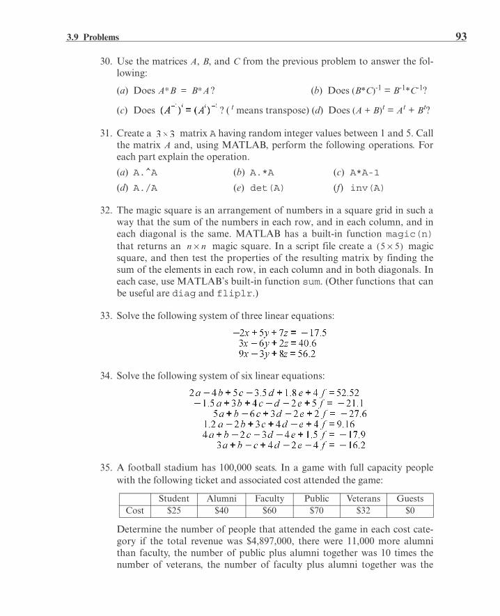
3.9 Problems 93
30. Use the matrices A, B, and C from the previous problem to answer the fol-lowing:
(a) Does ? (b) Does (B*C)-1 = B-1*C-1?
(c) Does ? ( t means transpose) (d) Does (A + B)t = At + Bt?
31. Create a matrix A having random integer values between 1 and 5. Callthe matrix A and, using MATLAB, perform the following operations. Foreach part explain the operation.
(a) A.^A (b) A.*A (c) A*A-1
(d) A./A (e) det(A) (f) inv(A)
32. The magic square is an arrangement of numbers in a square grid in such away that the sum of the numbers in each row, and in each column, and ineach diagonal is the same. MATLAB has a built-in function magic(n)that returns an magic square. In a script file create a magicsquare, and then test the properties of the resulting matrix by finding thesum of the elements in each row, in each column and in both diagonals. Ineach case, use MATLAB’s built-in function sum. (Other functions that canbe useful are diag and fliplr.)
33. Solve the following system of three linear equations:
34. Solve the following system of six linear equations:
35. A football stadium has 100,000 seats. In a game with full capacity peoplewith the following ticket and associated cost attended the game:
Determine the number of people that attended the game in each cost cate-gory if the total revenue was $4,897,000, there were 11,000 more alumnithan faculty, the number of public plus alumni together was 10 times thenumber of veterans, the number of faculty plus alumni together was the
Student Alumni Faculty Public Veterans GuestsCost $25 $40 $60 $70 $32 $0
A B B A=
n n 5 5

94 Chapter 3: Mathematical Operations with Arrays
same as the number of students, and the number of faculty plus studentstogether was four times larger than the number of guests and veteranstogether.
36. A food company manufactures five types of 8-oz trail mix packages usingdifferent mixtures of peanuts, almonds, walnuts, raisins, and M&Ms. Themixtures have the following compositions:
How many packages of each mix can be manufactured if 105 lb of peanuts,74 lb of almonds, 102 lb of walnuts, 118 lb of raisins, and 121 lb of M&Msare available? Write a system of linear equations and solve.
37. The electrical circuit shown consists ofresistors and voltage sources. Determine
and , using the mesh currentmethod based on Kirchhoff’s voltagelaw (see Sample Problem 3-4).
V, V, V
, ,
, ,
,
Peanuts (oz)
Almonds (oz)
Walnuts (oz)
Raisins (oz)
M&Ms (oz)
Mix 1 3 1 1 2 1Mix 2 1 2 1 3 1Mix 3 1 1 0 3 3Mix 4 2 0 3 1 2Mix 5 1 2 3 0 2
R1 R2
R3
R5R4
V1
V3
R6 R7
R8+ _
i1 i2 i3
i4
V2
+
+
_
_

95
Chapter 4 Using Script Files and Managing Data
A script file (see Section 1.8) is a list of MATLAB commands, called a program,that is saved in a file. When the script file is executed (run), MATLAB executesthe commands. Section 1.8 describes how to create, save, and run a simple scriptfile in which the commands are executed in the order in which they are listed,and in which all the variables are defined within the script file. This chapter givesmore details about how to input data to a script file, how data is stored in MAT-LAB, various ways to display and save data that is created in script files, andhow to exchange data between MATLAB and other applications. (How to writemore advanced programs in which commands are not necessarily executed in asimple order is covered in Chapter 6.)
In general, variables can be defined (created) in several ways. As shown inChapter 2, variables can be defined implicitly by assigning values to a variablename. Variables can also be assigned values by the output of a function. In addi-tion, variables can be defined with data that is imported from files outsideMATLAB. Once defined (either in the Command Window or when a script fileis executed), the variables are stored in MATLAB’s Workspace.
Variables that reside in the workspace can be displayed in various ways,saved, or exported to applications outside MATLAB. Similarly, data from filesoutside MATLAB can be imported to the workspace and then used in MAT-LAB.
Section 4.1 explains how MATLAB stores data in the workspace and howthe user can see the data that is stored. Section 4.2 shows how variables that areused in script files can be defined in the Command Window and/or in scriptfiles. Section 4.3 shows how to output data that is generated when script files areexecuted. Section 4.4 explains how the variables in the workspace can be savedand then retrieved, and Section 4.5 shows how to import and export data fromand to applications outside MATLAB.
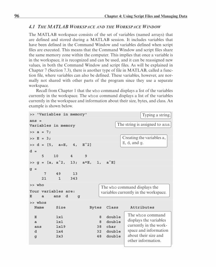
96 Chapter 4: Using Script Files and Managing Data
4.1 THE MATLAB WORKSPACE AND THE WORKSPACE WINDOW
The MATLAB workspace consists of the set of variables (named arrays) thatare defined and stored during a MATLAB session. It includes variables thathave been defined in the Command Window and variables defined when scriptfiles are executed. This means that the Command Window and script files sharethe same memory zone within the computer. This implies that once a variable isin the workspace, it is recognized and can be used, and it can be reassigned newvalues, in both the Command Window and script files. As will be explained inChapter 7 (Section 7.3), there is another type of file in MATLAB, called a func-tion file, where variables can also be defined. These variables, however, are nor-mally not shared with other parts of the program since they use a separateworkspace.
Recall from Chapter 1 that the who command displays a list of the variablescurrently in the workspace. The whos command displays a list of the variablescurrently in the workspace and information about their size, bytes, and class. Anexample is shown below.
>> 'Variables in memory'
ans =Variables in memory
>> a = 7;
>> E = 3;
>> d = [5, a+E, 4, E^2]
d = 5 10 4 9
>> g = [a, a^2, 13; a*E, 1, a^E]
g = 7 49 13 21 1 343
>> who
Your variables are:E a ans d g
>> whos Name Size Bytes Class Attributes
E 1x1 8 double a 1x1 8 double ans 1x19 38 char d 1x4 32 double g 2x3 48 double
Typing a string.
The string is assigned to ans.
Creating the variables a, E, d, and g.
The who command displays the variables currently in the workspace.
The whos command displays the variables currently in the work-space and information about their size and other information.

4.2 Input to a Script File 97
The variables currently in memory can also be viewed in the WorkspaceWindow. This window can be opened by selecting Workspace in the Desktopmenu. Figure 4-1 shows the Workspace Window that corresponds to the vari-ables defined above. The variables that are displayed in the Workspace Window
can also be edited (changed). Double-clicking on a variable opens the VariableEditor Window, where the content of the variable is displayed in a table. Forexample, Figure 4-2 shows the Variable Editor Window that opens when thevariable g in Figure 4-1 is double-clicked.
The elements in the Variable Editor Window can be edited. The variables in theWorkspace Window can be deleted by selecting them, and then either pressingthe delete key on the keyboard or selecting delete from the edit menu. This hasthe same effect as entering the command clear variable_name in theCommand Window.
4.2 INPUT TO A SCRIPT FILE
When a script file is executed, the variables that are used in the calculationswithin the file must have assigned values. In other words, the variables must bein the workspace. The assignment of a value to a variable can be done in threeways, depending on where and how the variable is defined.
Figure 4-1: The Workspace Window.
Figure 4-2: The Variable Editor Window.

98 Chapter 4: Using Script Files and Managing Data
1. The variable is defined and assigned a value in the script file.
In this case the assignment of a value to the variable is part of the script file. Ifthe user wants to run the file with a different variable value, the file must beedited and the assignment of the variable changed. Then, after the file is saved, itcan be executed again.
The following is an example of such a case. The script file (saved as Chap-ter4Example2) calculates the average points scored in three games.
The display in the Command Window when the script file is executed is:
2. The variable is defined and assigned a value in the Command Window.
In this case the assignment of a value to the variable is done in the CommandWindow. (Recall that the variable is recognized in the script file.) If the userwants to run the script file with a different value for the variable, the new value isassigned in the Command Window and the file is executed again.
For the previous example in which the script file has a program that calcu-lates the average of points scored in three games, the script file (saved as Chap-ter4Example3) is:
The Command Window for running this file is:
% The script file calculates the average points scored in three games.
% The assignment of the values of the points is part of the script file.
game1=75;
game2=93;
game3=68;
ave_points=(game1+game2+game3)/3
>> Chapter4Example2
ave_points = 78.6667>>
% The script file calculates the average points scored in three games.
% The assignment of the values of the points to the variables
% game1, game2, and game3 is done in the Command Window.
ave_points=(game1+game2+game3)/3
>> game1 = 67;>> game2 = 90;>> game3 = 81;
The variables are assigned values within the script file.
The script file is executed by typing the name of the file.
The variable ave_points with its valueis displayed in the Command Window.
The variables are assigned values in the Command Window.

4.2 Input to a Script File 99
3. The variable is defined in the script file, but a specific value is enteredin the Command Window when the script file is executed.
In this case the variable is defined in the script file, and when the file is executed,the user is prompted to assign a value to the variable in the Command Window.This is done by using the input command for creating the variable.
The form of the input command is:
When the input command is executed as the script file runs, the string is dis-played in the Command Window. The string is a message prompting the user toenter a value that is assigned to the variable. The user types the value andpresses the Enter key. This assigns the value to the variable. As with any variable,the variable and its assigned value will be displayed in the Command Windowunless a semicolon is typed at the very end of the input command. A script filethat uses the input command to enter the points scored in each game to theprogram that calculates the average of the scores is shown below.
>> pChater4Example3
ave_points = 79.3333
>> game1 = 87;>> game2 = 70;>> game3 = 50;
>> Chapter4Example3
ave_points = 69>>
% This script file calculates the average of points scored inthree games.
% The points from each game are assigned to the variables by
% using the input command.
game1=input('Enter the points scored in the first game ');
game2=input('Enter the points scored in the second game ');
game3=input('Enter the points scored in the third game ');
ave_points=(game1+game2+game3)/3
The script file is executed.
The output from the script file is dis-played in the Command Window.
New values are assigned to the variables.
The script file is executed again.
The output from the script file is dis-played in the Command Window.
variable_name = input(‘string with a message that is displayed in the Command Window’)

100 Chapter 4: Using Script Files and Managing Data
The following shows the Command Window when this script file (saved asChapter4Example4) is executed.
In this example scalars are assigned to the variables. In general, however,vectors and arrays can also be assigned. This is done by typing the array in thesame way that it is usually assigned to a variable (left bracket, then typing rowby row, and a right bracket).
The input command can also be used to assign a string to a variable. Thiscan be done in one of two ways. One way is to use the command in the sameform as shown above, and when the prompt message appears the string is typedbetween two single quotes in the same way that a string is assigned to a variablewithout the input command. The second way is to use an option in the inputcommand that defines the characters that are entered as a string. The form ofthe command is:
where the ‘s’ inside the command defines the characters that will be entered asa string. In this case when the prompt message appears, the text is typed in with-out the single quotes, but it is assigned to the variable as a string. An examplewhere the input command is used with this option is included in Sample Prob-lem 6-4.
4.3 OUTPUT COMMANDS
As discussed before, MATLAB automatically generates a display when somecommands are executed. For example, when a variable is assigned a value, or thename of a previously assigned variable is typed and the Enter key is pressed,MATLAB displays the variable and its value. This type of output is not dis-played if a semicolon is typed at the end of the command. In addition to thisautomatic display, MATLAB has several commands that can be used to gener-ate displays. The displays can be messages that provide information, numericaldata, and plots. Two commands that are frequently used to generate output aredisp and fprintf. The disp command displays the output on the screen,while the fprintf command can be used to display the output on the screen orto save the output to a file. The commands can be used in the Command Win-
>> Chapter4Example4
Enter the points scored in the first game 67
Enter the points scored in the second game 91Enter the points scored in the third game 70
ave_points = 76>>
The computer dis-plays the message. Then the value of the score is typed by the user and the Enter key is pressed.
variable_name = input(‘prompt message’,‘s’)
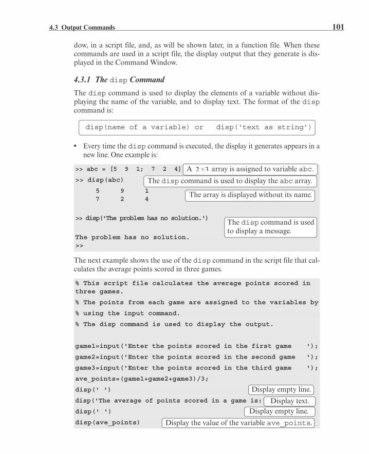
4.3 Output Commands 101
dow, in a script file, and, as will be shown later, in a function file. When thesecommands are used in a script file, the display output that they generate is dis-played in the Command Window.
4.3.1 The disp Command
The disp command is used to display the elements of a variable without dis-playing the name of the variable, and to display text. The format of the dispcommand is:
• Every time the disp command is executed, the display it generates appears in anew line. One example is:
The next example shows the use of the disp command in the script file that cal-culates the average points scored in three games.
>> abc = [5 9 1; 7 2 4];
>> disp(abc)
5 9 1 7 2 4
>> disp('The problem has no solution.')
The problem has no solution.>>
% This script file calculates the average points scored in three games.
% The points from each game are assigned to the variables by
% using the input command.
% The disp command is used to display the output.
game1=input('Enter the points scored in the first game ');
game2=input('Enter the points scored in the second game ');
game3=input('Enter the points scored in the third game ');
ave_points=(game1+game2+game3)/3;
disp(' ')
disp('The average of points scored in a game is:')
disp(' ')
disp(ave_points)
disp(name of a variable) or disp(‘text as string’)
A array is assigned to variable abc.
The disp command is used to display the abc array.
The array is displayed without its name.
The disp command is usedto display a message.
Display empty line.
Display text.Display empty line.
Display the value of the variable ave_points.

102 Chapter 4: Using Script Files and Managing Data
When this file (saved as Chapter4Example5) is executed, the display in theCommand Window is:
• Only one variable can be displayed in a disp command. If elements of two vari-ables need to be displayed together, a new variable (that contains the elements tobe displayed) must first be defined and then displayed.
In many situations it is nice to display output (numbers) in a table. This canbe done by first defining a variable that is an array with the numbers and thenusing the disp command to display the array. Headings to the columns canalso be created with the disp command. Since in the disp command the usercannot control the format (the width of the columns and the distance betweenthe columns) of the display of the array, the position of the headings has to bealigned with the columns by adding spaces. As an example, the script file belowshows how to display the population data from Chapter 2 in a table.
When this script file (saved as PopTable) is executed, the display in the Com-mand Window is:
>> Chapter4Example5
Enter the points scored in the first game 89
Enter the points scored in the second game 60
Enter the points scored in the third game 82
The average of points scored in a game is:
77
yr=[1984 1986 1988 1990 1992 1994 1996];
pop=[127 130 136 145 158 178 211];
tableYP(:,1)=yr';
tableYP(:,2)=pop';
disp(' YEAR POPULATION')
disp(' (MILLIONS)')
disp(' ')
disp(tableYP)
>> PopTable
YEAR POPULATION (MILLIONS)
1984 127
An empty line is displayed.
The text line is displayed.
An empty line is displayed.
The value of the variable ave_points is displayed.
The population data is entered in two row vectors.
yr is entered as the first column in the array tableYP.
pop is entered as the second column in the array tableYP.
Display heading (first line).
Display heading (second line).
Display an empty line.
Display the array tableYP.
Headings are displayed.
An empty line is displayed.
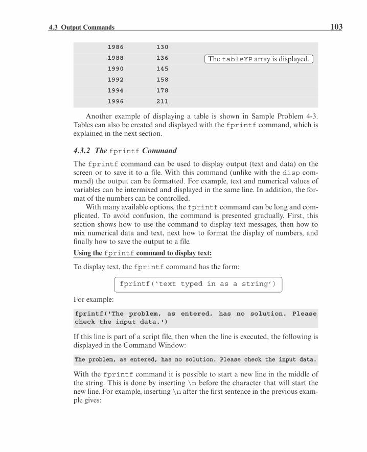
4.3 Output Commands 103
Another example of displaying a table is shown in Sample Problem 4-3.Tables can also be created and displayed with the fprintf command, which isexplained in the next section.
4.3.2 The fprintf Command
The fprintf command can be used to display output (text and data) on thescreen or to save it to a file. With this command (unlike with the disp com-mand) the output can be formatted. For example, text and numerical values ofvariables can be intermixed and displayed in the same line. In addition, the for-mat of the numbers can be controlled.
With many available options, the fprintf command can be long and com-plicated. To avoid confusion, the command is presented gradually. First, thissection shows how to use the command to display text messages, then how tomix numerical data and text, next how to format the display of numbers, andfinally how to save the output to a file.
Using the fprintf command to display text:
To display text, the fprintf command has the form:
For example:
If this line is part of a script file, then when the line is executed, the following isdisplayed in the Command Window:
With the fprintf command it is possible to start a new line in the middle ofthe string. This is done by inserting \n before the character that will start thenew line. For example, inserting \n after the first sentence in the previous exam-ple gives:
1986 130
1988 136
1990 145
1992 158
1994 178
1996 211
fprintf('The problem, as entered, has no solution. Pleasecheck the input data.')
The problem, as entered, has no solution. Please check the input data.
The tableYP array is displayed.
fprintf(‘text typed in as a string’)

104 Chapter 4: Using Script Files and Managing Data
When this line executes, the display in the Command Window is:
The \n is called an escape character. It is used to control the display. Otherescape characters that can be inserted within the string are:
\b Backspace.\t Horizontal tab.
When a program has more than one fprintf command, the display gener-ated is continuous (the fprintf command does not automatically start a newline). This is true even if there are other commands between the fprintf com-mands. An example is the following script file:
When this file is executed the display in the Command Window is:
To start a new line with the fprintf command, \n must be typed at the startof the string.
Using the fprintf command to display a mix of text and numerical data:
To display a mix of text and a number (value of a variable), the fprintf com-mand has the form:
fprintf('The problem, as entered, has no solution.\nPleasecheck the input data.')
The problem, as entered, has no solution.Please check the input data.
fprintf('The problem, as entered, has no solution. Pleasecheck the input data.')
x = 6; d = 19 + 5*x;
fprintf('Try to run the program later.')
y = d + x;
fprintf('Use different input values.')
The problem, as entered, has no solution. Please check theinput data.Try to run the program later.Use different inputvalues.
fprintf(‘text as string %-5.2f additional text’, variable_name)
The name of the variable whose value is displayed.
Formatting elements (define the format of the number).
The % sign marks the spot where the number is inserted within the text.

4.3 Output Commands 105
The formatting elements are:
The flag, which is optional, can be one of the following three characters:
The field width and precision (5.2 in the previous example) are optional.The first number (5 in the example) is the field width, which specifies the mini-mum number of digits in the display. If the number to be displayed is shorterthan the field width, spaces or zeros are added in front of the number. The preci-sion is the second number (2 in the example). It specifies the number of digits tobe displayed to the right of the decimal point.
The last element in the formatting elements, which is required, is the conver-sion character, which specifies the notation in which the number is displayed.Some of the common notations are:
e Exponential notation using lowercase e (e.g., 1.709098e+001).E Exponential notation using uppercase E (e.g., 1.709098E+001).f Fixed-point notation (e.g., 17.090980).g The shorter of e or f notations.G The shorter of E or f notations. i Integer.
Information about additional notation is available in the help menu of MAT-LAB. As an example, the fprintf command with a mix of text and a numberis used in the script file that calculates the average points scored in three games.
Character used for flag
Description
– (minus sign) Left-justifies the number within the field.+ (plus sign) Prints a sign character (+ or –) in front of the number.
0 (zero) Adds zeros if the number is shorter than the field.
% This script file calculates the average points scored in three games.
% The values are assigned to the variables by using the input command.
% The fprintf command is used to display the output.
game(1) = input('Enter the points scored in the first game ');
game(2) = input('Enter the points scored in the second game ');
game(3) = input('Enter the points scored in the third game ');
ave_points = mean(game);
–5.2f
Conversion character(required)
Field width and precision(optional)
Flag(optional)

106 Chapter 4: Using Script Files and Managing Data
Notice that, besides using the fprintf command, this file differs from the onesshown earlier in the chapter in that the scores are stored in the first three ele-ments of a vector named game, and the average of the scores is calculated byusing the mean function. The Command Window where the script file above(saved as Chapter4Example6) was run is shown below.
With the fprintf command it is possible to insert more than one number(value of a variable) within the text. This is done by typing %g (or % followed byany formatting elements) at the places in the text where the numbers are to beinserted. Then, after the string argument of the command (following thecomma), the names of the variables are typed in the order in which they areinserted in the text. In general the command looks like:
An example is shown in the following script file:
fprintf('An average of %f points was scored in the three games.',ave_points)
>> Chapter4Example6
Enter the points scored in the first game 75
Enter the points scored in the second game 60
Enter the points scored in the third game 81
An average of 72.000000 points was scored in the three games.>>
% This program calculates the distance a projectile flies,
% given its initial velocity and the angle at which it is shot.
% the fprintf command is used to display a mix of text and num-bers.
v=1584; % Initial velocity (km/h)
theta=30; % Angle (degrees)
vms=v*1000/3600;
t=vms*sind(30)/9.81;
d=vms*cosd(30)*2*t/1000;
Text Additionaltext.
% marks the position of the number.
The name of the variable whose value is displayed.
The display generated by the fprintf commandcombines text and a number (value of a variable).
fprintf(‘..text...%g...%g...%f...’,variable1,variable2,variable3)
Changing velocity units to m/s.
Calculating the time to highest point.
Calculating max distance.
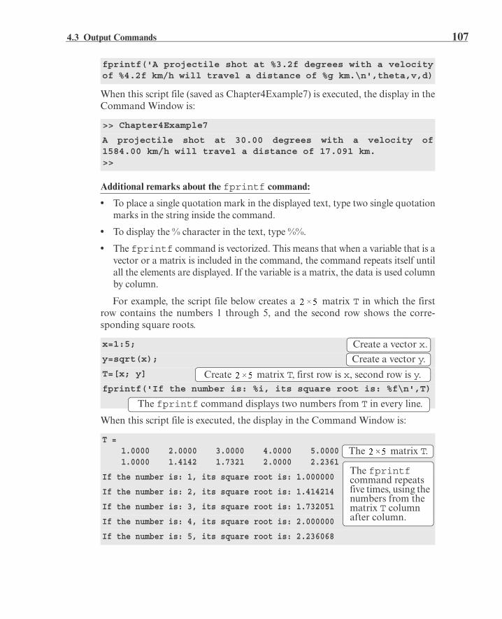
4.3 Output Commands 107
When this script file (saved as Chapter4Example7) is executed, the display in theCommand Window is:
Additional remarks about the fprintf command:
• To place a single quotation mark in the displayed text, type two single quotationmarks in the string inside the command.
• To display the % character in the text, type %%.
• The fprintf command is vectorized. This means that when a variable that is avector or a matrix is included in the command, the command repeats itself untilall the elements are displayed. If the variable is a matrix, the data is used columnby column.
For example, the script file below creates a matrix T in which the firstrow contains the numbers 1 through 5, and the second row shows the corre-sponding square roots.
When this script file is executed, the display in the Command Window is:
fprintf('A projectile shot at %3.2f degrees with a velocityof %4.2f km/h will travel a distance of %g km.\n',theta,v,d)
>> Chapter4Example7
A projectile shot at 30.00 degrees with a velocity of1584.00 km/h will travel a distance of 17.091 km.>>
x=1:5;
y=sqrt(x);
T=[x; y]
fprintf('If the number is: %i, its square root is: %f\n',T)
T = 1.0000 2.0000 3.0000 4.0000 5.0000 1.0000 1.4142 1.7321 2.0000 2.2361
If the number is: 1, its square root is: 1.000000
If the number is: 2, its square root is: 1.414214
If the number is: 3, its square root is: 1.732051
If the number is: 4, its square root is: 2.000000
If the number is: 5, its square root is: 2.236068
Create a vector x.
Create a vector y.
Create matrix T, first row is x, second row is y.
The fprintf command displays two numbers from T in every line.
The matrix T.
The fprintf command repeats five times, using the numbers from the matrix T column after column.

108 Chapter 4: Using Script Files and Managing Data
Using the fprintf command to save output to a file:
In addition to displaying output in the Command Window, the fprintf com-mand can be used for writing the output to a file when it is necessary to save theoutput. The data that is saved can subsequently be displayed or used in MAT-LAB and in other applications.
Writing output to a file requires three steps:
a) Opening a file using the fopen command.b) Writing the output to the open file using the fprintf command.c) Closing the file using the fclose command.
Step a:
Before data can be written to a file, the file must be opened. This is done withthe fopen command, which creates a new file or opens an existing file. Thefopen command has the form:
fid is a variable called the file identifier. A scalar value is assigned to fid whenfopen is executed. The file name is written (including its extension) within sin-gle quotes as a string. The permission is a code (also written as a string) thattells how the file is opened. Some of the more common permission codes are:
‘r’ Open file for reading (default).‘w’ Open file for writing. If the file already exists, its
content is deleted. If the file does not exist, a new file is created.‘a’ Same as ‘w’, except that if the file exists the written
data is appended to the end of the file.‘r+’ Open (do not create) file for reading and writing.‘w+’ Open file for reading and writing. If the file already
exists, its content is deleted. If the file does not exist, a new file iscreated.
‘a+’ Same as ‘w+’, except that if the file exists the writ-ten data is appended to the end of the file.
If a permission code is not included in the command, the file opens with thedefault code ‘r’. Additional permission codes are described in the help menu.
Step b:
Once the file is open, the fprintf command can be used to write output to thefile. The fprintf command is used in exactly the same way as it is used to dis-play output in the Command Window, except that the variable fid is insertedinside the command. The fprintf command then has the form:
fid = fopen(‘file_name’,‘permission’)
fprintf(fid,‘text %-5.2f additional text’,vari able_name)
fid is added to the fprintf command.

4.3 Output Commands 109
Step c:
When the writing of data to the file is complete, the file is closed using thefclose command. The fclose command has the form:
Additional notes on using the fprintf command for saving output to a file:
• The created file is saved in the current directory.
• It is possible to use the fprintf command to write to several different files.This is done by first opening the files, assigning a different fid to each (e.g.fid1, fid2, fid3, etc.), and then using the fid of a specific file in thefprintf command to write to that file.
An example of using fprintf commands for saving output to two files isshown in the following script file. The program in the file generates two unit con-version tables. One table converts velocity units from miles per hour to kilome-ters per hour, and the other table converts force units from pounds to newtons.Each conversion table is saved to a different text file (extension .txt).
% Script file in which fprintf is used to write output to files.
% Two conversion tables are created and saved to two different files.
% One converts mi/h to km/h, the other converts lb to N.
clear all
Vmph=10:10:100;
Vkmh=Vmph.*1.609;
TBL1=[Vmph; Vkmh];
Flb=200:200:2000;
FN=Flb.*4.448;
TBL2=[Flb; FN];
fid1=fopen('VmphtoVkm.txt','w');
fid2=fopen('FlbtoFN.txt','w');
fprintf(fid1,'Velocity Conversion Table\n \n');
fprintf(fid1,' mi/h km/h \n');
fprintf(fid1,' %8.2f %8.2f\n',TBL1);
fclose(fid)
Creating a vector of velocities in mi/h.
Converting mph to km/h.
Creating a table (matrix) with two rows.
Creating a vector of forces in lb.
Converting lb to N.
Creating a table (matrix) with two rows.
Open a .txt file named VmphtoVkm.
Open a .txt file named FlbtoFN.
Writing a title and an empty line to the file fid1.
Writing two column headings to the file fid1.
Writing the data from the variable TBL1 to the file fid1.
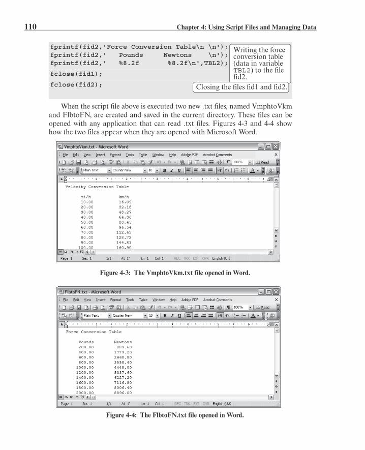
110 Chapter 4: Using Script Files and Managing Data
When the script file above is executed two new .txt files, named VmphtoVkmand FlbtoFN, are created and saved in the current directory. These files can beopened with any application that can read .txt files. Figures 4-3 and 4-4 showhow the two files appear when they are opened with Microsoft Word.
fprintf(fid2,'Force Conversion Table\n \n');fprintf(fid2,' Pounds Newtons \n');fprintf(fid2,' %8.2f %8.2f\n',TBL2);
fclose(fid1);
fclose(fid2);
Figure 4-3: The VmphtoVkm.txt file opened in Word.
Figure 4-4: The FlbtoFN.txt file opened in Word.
Writing the force conversion table (data in variable TBL2) to the file fid2.
Closing the files fid1 and fid2.
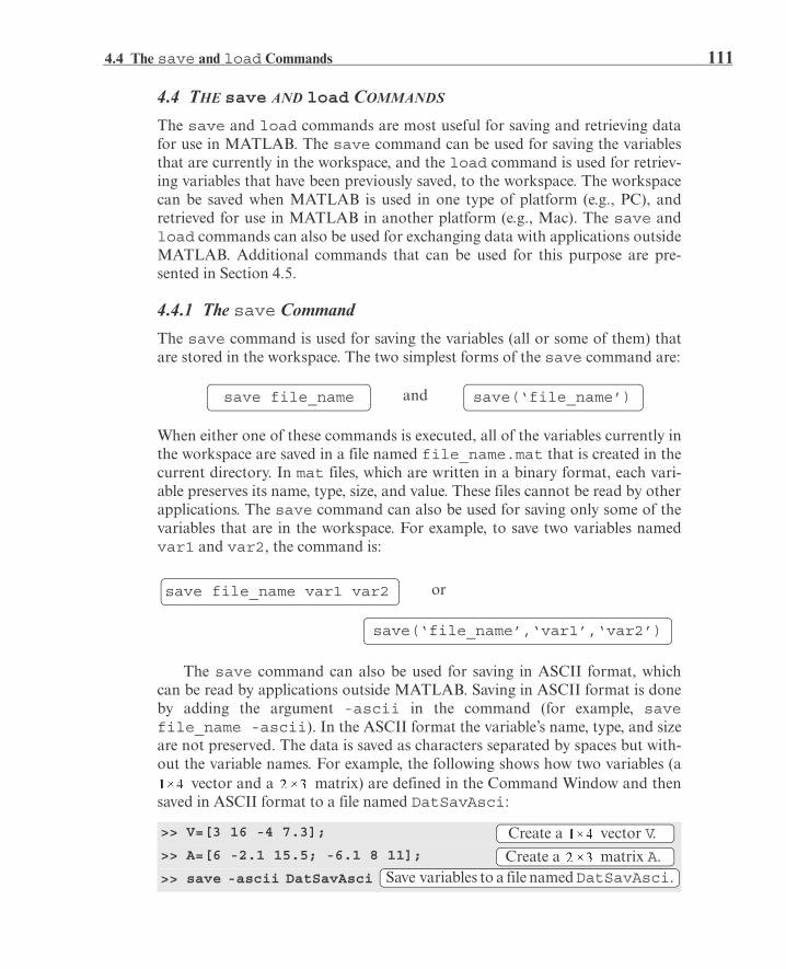
4.4 The save and load Commands 111
4.4 THE save AND load COMMANDS
The save and load commands are most useful for saving and retrieving datafor use in MATLAB. The save command can be used for saving the variablesthat are currently in the workspace, and the load command is used for retriev-ing variables that have been previously saved, to the workspace. The workspacecan be saved when MATLAB is used in one type of platform (e.g., PC), andretrieved for use in MATLAB in another platform (e.g., Mac). The save andload commands can also be used for exchanging data with applications outsideMATLAB. Additional commands that can be used for this purpose are pre-sented in Section 4.5.
4.4.1 The save Command
The save command is used for saving the variables (all or some of them) thatare stored in the workspace. The two simplest forms of the save command are:
When either one of these commands is executed, all of the variables currently inthe workspace are saved in a file named file_name.mat that is created in thecurrent directory. In mat files, which are written in a binary format, each vari-able preserves its name, type, size, and value. These files cannot be read by otherapplications. The save command can also be used for saving only some of thevariables that are in the workspace. For example, to save two variables namedvar1 and var2, the command is:
The save command can also be used for saving in ASCII format, whichcan be read by applications outside MATLAB. Saving in ASCII format is doneby adding the argument -ascii in the command (for example, savefile_name -ascii). In the ASCII format the variable’s name, type, and sizeare not preserved. The data is saved as characters separated by spaces but with-out the variable names. For example, the following shows how two variables (a
vector and a matrix) are defined in the Command Window and thensaved in ASCII format to a file named DatSavAsci:
>> V=[3 16 -4 7.3];
>> A=[6 -2.1 15.5; -6.1 8 11];
>> save -ascii DatSavAsci
save file_name save(‘file_name’)and
save file_name var1 var2
save(‘file_name’,‘var1’,‘var2’)
or
Create a vector V.
Create a matrix A.Save variables to a file named DatSavAsci.

112 Chapter 4: Using Script Files and Managing Data
Once saved, the file can be opened by any application that can read ASCII files.For example, Figure 4-5 shows the data when the file is opened with Notepad.
Note that the file does not include the names of the variables, just the numericalvalues of the variables (first A and then V) are listed.
4.4.2 The load Command
The load command can be used for retrieving variables that were saved withthe save command back to the workspace, and for importing data that was cre-ated with other applications and saved in ASCII format or in text (.txt) files.Variables that were saved with the save command in .mat files can be retrievedwith the command:
When the command is executed, all the variables in the file (with the name, type,size, and values as were saved) are added (loaded back) to the workspace. If theworkspace already has a variable with the same name as a variable that isretrieved with the load command, then the variable that is retrieved replacesthe existing variable. The load command can also be used for retrieving onlysome of the variables that are in the saved .mat file. For example, to retrieve twovariables named var1 and var2, the command is:
The load command can also be used to import data that is saved in ASCIIor text (.txt) to the workspace. This is possible, however, only if the data in thefile is in the form of a variable in MATLAB. Thus, the file can have one number(scalar), a row or a column of numbers (vector), or rows with the same numberof numbers in each (matrix). For example, the data shown in Figure 4-5 cannotbe loaded with the load command (even though it was saved in ASCII formatwith the save command), because the number of elements is not the same in allrows. (Recall that this file was created by saving two different variables.)
Figure 4-5: Data saved in ASCII format.
load file_name load(‘file_name’)or
load file_name var1 var2
load(‘file_name’,‘var1’,‘var2’)
or

4.4 The save and load Commands 113
When data is loaded from an ASCII or text file into the workspace, it has tobe assigned to a variable name. Data in ASCII format can be loaded with eitherof the following two forms of the load command:
If the data is in a text file, the extension .txt has to be added to the file name. Theform of the load command is then:
In the first form of the command the data is assigned to a variable that has thename of the file. In the second form the data is assigned to a variable namedVarName.
For example, the data shown in Figure 4-6 (a matrix) is typed inNotepad, and then saved as DataFromText.txt.
Next, two forms of the load command are used to import the data in thetext file to the Workspace of MATLAB. In the first command the data isassigned to a variable named DfT. In the second command the data is automat-ically assigned to a variable named DataFromText, which is the name of thetext file where the data was saved.
Importing data to (or exporting from) other applications can also be done, withMATLAB commands that are presented in the next section.
Figure 4-6: Data saved as .txt file.
>> DfT=load('DataFromText.txt')
DfT = 56.0000 -4.2000 3.0000 7.5000 -1.6000 198.0000
>> load DataFromText.txt
>> DataFromTextDataFromText = 56.0000 -4.2000 3.0000 7.5000 -1.6000 198.0000
load file_name VarName=load(‘file_name’)or
load file_name.txt VarName=load(‘file_name.txt’)or
Load the file DataFromText and assign the loaded data to the variable Dft.
Use the load command with the file DataFromText.
The data is assigned to a vari-able named DataFromText.

114 Chapter 4: Using Script Files and Managing Data
4.5 IMPORTING AND EXPORTING DATA
MATLAB is often used for analyzing data that was recorded in experiments orgenerated by other computer programs. This can be done by first importing thedata into MATLAB. Similarly, data that is produced by MATLAB sometimesneeds to be transferred to other computer applications. There are various typesof data (numerical, text, audio, graphics, and images). This section describesonly how to import and export numerical data, which is probably the most com-mon type of data that needs to be transferred by new users of MATLAB. Forother types of data transfer, look in the Help Window under File I/O.
Importing data can be done either by using commands or by using theImport Wizard. Commands are useful when the format of the data beingimported is known. MATLAB has several commands that can be used forimporting various types of data. Importing commands can also be included in ascript file such that the data is imported when the script is executed. The ImportWizard is useful when the format of the data (or the command that is applicablefor importing the data) is not known. The Import Wizard determines the formatof the data and automatically imports it.
4.5.1 Commands for Importing and Exporting Data
This section describes—in detail—how to transfer data into and out of Excelspreadsheets. Microsoft Excel is commonly used for storing data, and Excel iscompatible with many data recording devices and computer applications. Manypeople are also capable of importing and exporting various data formats intoand from Excel. MATLAB also has commands for transferring data directly toand from formats such as csv and ASCII, as well as to the spreadsheet programLotus 123. Details of these and many other commands can be found in the HelpWindow under File I/O
Importing and exporting data into and from Excel:
Importing data from Excel is done with the xlsread command. When thecommand is executed, the data from the spreadsheet is assigned as an array to avariable. The simplest form of the xlsread command is:
• ‘filename’ (typed as a string) is the name of the Excel file. The directory ofthe Excel file must be either the current directory or listed in the search path.
• If the Excel file has more than one sheet, the data will be imported from the firstsheet.
variable_name = xlsread(‘filename’)
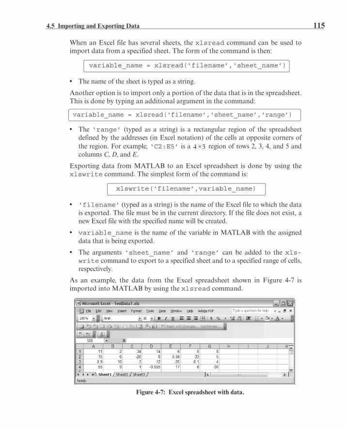
4.5 Importing and Exporting Data 115
When an Excel file has several sheets, the xlsread command can be used toimport data from a specified sheet. The form of the command is then:
• The name of the sheet is typed as a string.
Another option is to import only a portion of the data that is in the spreadsheet.This is done by typing an additional argument in the command:
• The ‘range’ (typed as a string) is a rectangular region of the spreadsheetdefined by the addresses (in Excel notation) of the cells at opposite corners ofthe region. For example, ‘C2:E5’ is a region of rows 2, 3, 4, and 5 andcolumns C, D, and E.
Exporting data from MATLAB to an Excel spreadsheet is done by using thexlswrite command. The simplest form of the command is:
• ‘filename’ (typed as a string) is the name of the Excel file to which the datais exported. The file must be in the current directory. If the file does not exist, anew Excel file with the specified name will be created.
• variable_name is the name of the variable in MATLAB with the assigneddata that is being exported.
• The arguments ‘sheet_name’ and ‘range’ can be added to the xls-write command to export to a specified sheet and to a specified range of cells,respectively.
As an example, the data from the Excel spreadsheet shown in Figure 4-7 isimported into MATLAB by using the xlsread command.
Figure 4-7: Excel spreadsheet with data.
variable_name = xlsread(‘filename’,‘sheet_name’)
variable_name = xlsread(‘filename’,‘sheet_name’,‘range’)
xlswrite(‘filename’,variable_name)
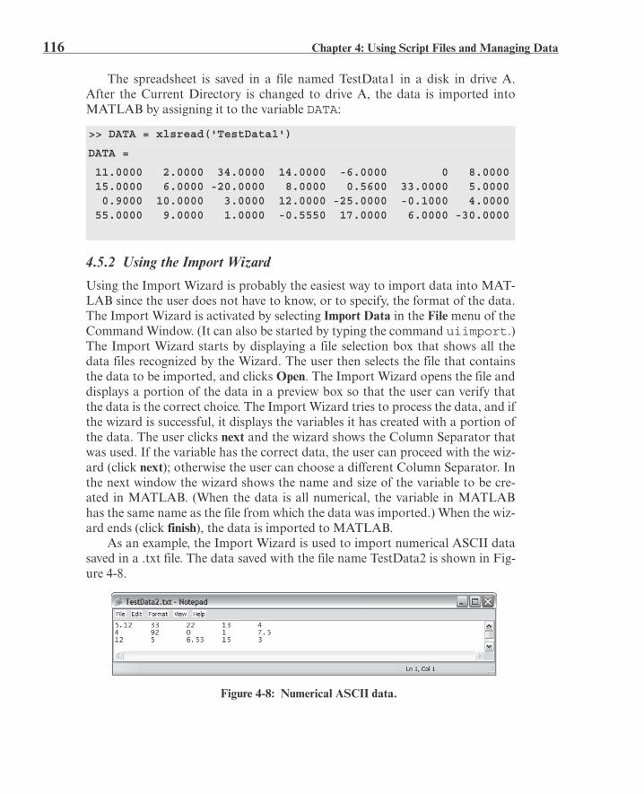
116 Chapter 4: Using Script Files and Managing Data
The spreadsheet is saved in a file named TestData1 in a disk in drive A.After the Current Directory is changed to drive A, the data is imported intoMATLAB by assigning it to the variable DATA:
4.5.2 Using the Import Wizard
Using the Import Wizard is probably the easiest way to import data into MAT-LAB since the user does not have to know, or to specify, the format of the data.The Import Wizard is activated by selecting Import Data in the File menu of theCommand Window. (It can also be started by typing the command uiimport.)The Import Wizard starts by displaying a file selection box that shows all thedata files recognized by the Wizard. The user then selects the file that containsthe data to be imported, and clicks Open. The Import Wizard opens the file anddisplays a portion of the data in a preview box so that the user can verify thatthe data is the correct choice. The Import Wizard tries to process the data, and ifthe wizard is successful, it displays the variables it has created with a portion ofthe data. The user clicks next and the wizard shows the Column Separator thatwas used. If the variable has the correct data, the user can proceed with the wiz-ard (click next); otherwise the user can choose a different Column Separator. Inthe next window the wizard shows the name and size of the variable to be cre-ated in MATLAB. (When the data is all numerical, the variable in MATLABhas the same name as the file from which the data was imported.) When the wiz-ard ends (click finish), the data is imported to MATLAB.
As an example, the Import Wizard is used to import numerical ASCII datasaved in a .txt file. The data saved with the file name TestData2 is shown in Fig-ure 4-8.
>> DATA = xlsread('TestData1')
DATA =
11.0000 2.0000 34.0000 14.0000 -6.0000 0 8.0000 15.0000 6.0000 -20.0000 8.0000 0.5600 33.0000 5.0000 0.9000 10.0000 3.0000 12.0000 -25.0000 -0.1000 4.0000 55.0000 9.0000 1.0000 -0.5550 17.0000 6.0000 -30.0000
Figure 4-8: Numerical ASCII data.

4.5 Importing and Exporting Data 117
The display of the Import Wizard during the import process for the TestData2file is shown in Figures 4-9 and 4-10. Figure 4-10 shows that the name of thevariable in MATLAB is TestData2 and its size is .
In the Command Window of MATLAB, the imported data can be displayed bytyping the name of the variable.
Figure 4-9: Import Wizard, first display.
Figure 4-10: Import Wizard, second display.
>> TestData2
TestData2 = 5.1200 33.0000 22.0000 13.0000 4.0000 4.0000 92.0000 0 1.0000 7.5000 12.0000 5.0000 6.5300 15.0000 3.0000

118 Chapter 4: Using Script Files and Managing Data
4.6 EXAMPLES OF MATLAB APPLICATIONS
Sample Problem 4-1: Height and surface area of a silo
A cylindrical silo with radius r has aspherical cap roof with radius R. Theheight of the cylindrical portion is H.Write a program in a script file that deter-mines the height H for given values of r, R,and the volume V. In addition, the pro-gram calculates the surface area of thesilo.
Use the program to calculate the heightand surface area of a silo with r = 30 ft, R= 45 ft, and a volume of 200,000 ft3.Assign values for r, R, and V in the Com-mand Window.
Solution
The total volume of the silo is obtained by adding the volume of the cylindricalpart and the volume of the spherical cap. The volume of the cylinder is given by
and the volume of the spherical cap is givenby:
where ,
and is calculated from .Using the equations above, the height, H, ofthe cylindrical part can be expressed by
The surface area of the silo is obtained byadding the surface areas of the cylindricalpart and the spherical cap.
A program in a script file that solves the problem is presented below:
theta=asin(r/R);
h=R*(1-cos(theta));
H
r
R
Vcyl r2H=
S Scyl Scap+ 2 rH 2 Rh+= =
Calculating .
Calculating h.
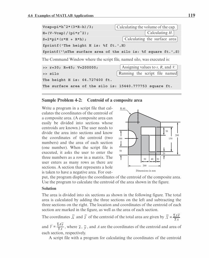
4.6 Examples of MATLAB Applications 119
The Command Window where the script file, named silo, was executed is:
Sample Problem 4-2: Centroid of a composite area
Write a program in a script file that cal-culates the coordinates of the centroid ofa composite area. (A composite area caneasily be divided into sections whosecentroids are known.) The user needs todivide the area into sections and knowthe coordinates of the centroid (twonumbers) and the area of each section(one number). When the script file isexecuted, it asks the user to enter thethree numbers as a row in a matrix. Theuser enters as many rows as there aresections. A section that represents a holeis taken to have a negative area. For out-put, the program displays the coordinates of the centroid of the composite area.Use the program to calculate the centroid of the area shown in the figure.
Solution
The area is divided into six sections as shown in the following figure. The totalarea is calculated by adding the three sections on the left and subtracting thethree sections on the right. The location and coordinates of the centroid of eachsection are marked in the figure, as well as the area of each section.
The coordinates and of the centroid of the total area are given by
and , where , , and A are the coordinates of the centroid and area of
each section, respectively.A script file with a program for calculating the coordinates of the centroid
Vcap=pi*h^2*(3*R-h)/3;
H=(V-Vcap)/(pi*r^2);
S=2*pi*(r*H + R*h);
fprintf('The height H is: %f ft.',H)
fprintf('\nThe surface area of the silo is: %f square ft.',S)
>> r=30; R=45; V=200000;
>> silo
The height H is: 64.727400 ft.
The surface area of the silo is: 15440.777753 square ft.
Calculating the volume of the cap. Calculating H.
Calculating the surface area
Assigning values to r, R, and V.
Running the script file named
200
3040
150200
50
50
100
50
20
R 60
Dimensions in mm

120 Chapter 4: Using Script Files and Managing Data
of a composite area is provided below.
The script file was saved with the name Centroid. The following shows the Com-mand Window where the script file was executed.
% The program calculates the coordinates of the centroid
% of a composite area.
clear C xs ys As
C=input('Enter a matrix in which each row has three ele-ments.\nIn each row enter the x and y coordinates of thecentroid and the area of a section.\n');
xs=C(:,1)';
ys=C(:,2)';
As=C(:,3)';
A=sum(As);
x=sum(As.*xs)/A;
y=sum(As.*ys)/A;
fprintf('The coordinates of the centroid are: ( %f, %f)\n',x,y)
>> Centroid
Enter a matrix in which each row has three elements.
In each row enter the x and y coordinates of the centroidand the area of a section.
Creating a row vector for the x coordinate of each section (first column of C).
Creating a row vector for the y coordinate of each section (second column of C).
Creating a row vector for the area of each section (third column of C).
Calculating the total area.
Calculating the coordinates of the centroid of the composite area.

4.6 Examples of MATLAB Applications 121
Sample Problem 4-3: Voltage divider
When several resistors are connected in an electrical circuit in series, the voltageacross each of them is given by the voltage divider rule:
where vn and Rn are the voltage across resistor n and its resistance, respectively,
is the equivalent resistance, and vs is the source voltage. The powerdissipated in each resistor is given by:
The figure below shows a circuit with seven resistors connected in series.
Write a program in a script file that calculates the voltage across each resistor,and the power dissipated in each resistor, in a circuit that has resistors connectedin series. When the script file is executed, it requests that the user first enter thesource voltage and then to enter the resistances of the resistors in a vector. Theprogram displays a table with the resistance listed in the first column, the volt-age across the resistor in the second column, and the power dissipated in theresistor in the third column. Following the table, the program displays the cur-rent in the circuit and the total power.
Execute the file and enter the following data for vs and the R’s.V, , , , , , ,
..
[100 100 200*20060-80/pi 200+80/pi pi*60^2/460+140/3 220 140*60/2200/(3*pi) 100 -pi*50^2/2105 145 -50*50150 95 -40*150]
The coordinates of the centroid are: ( 85.387547 , 131.211809 )
Entering the data for matrix C. Each row has three elements: the x, y, and A of a section.
+_
R1 R2 R3
vs R4
R5R6R7
vs 24= R1 20= R2 14= R3 12= R4 18= R5 8= R6 15=R7 10=
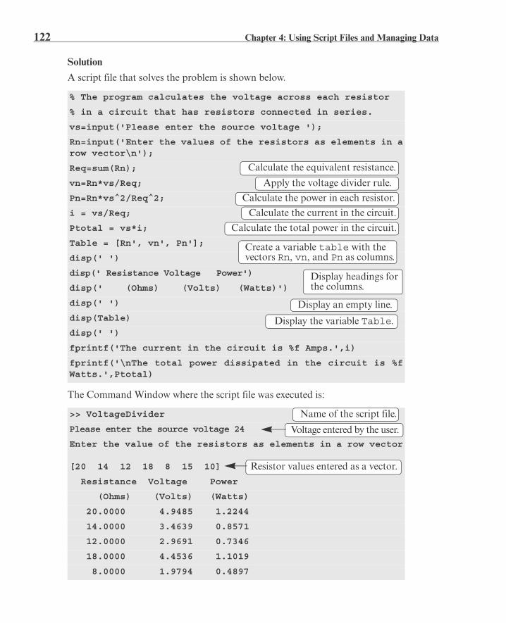
122 Chapter 4: Using Script Files and Managing Data
Solution
A script file that solves the problem is shown below.
The Command Window where the script file was executed is:
% The program calculates the voltage across each resistor
% in a circuit that has resistors connected in series.
vs=input('Please enter the source voltage ');
Rn=input('Enter the values of the resistors as elements in arow vector\n');
Req=sum(Rn);
vn=Rn*vs/Req;
Pn=Rn*vs^2/Req^2;
i = vs/Req;
Ptotal = vs*i;
Table = [Rn', vn', Pn'];
disp(' ')
disp(' Resistance Voltage Power')
disp(' (Ohms) (Volts) (Watts)')
disp(' ')
disp(Table)
disp(' ')
fprintf('The current in the circuit is %f Amps.',i)
fprintf('\nThe total power dissipated in the circuit is %fWatts.',Ptotal)
>> VoltageDivider
Please enter the source voltage 24
Enter the value of the resistors as elements in a row vector
[20 14 12 18 8 15 10]
Resistance Voltage Power
(Ohms) (Volts) (Watts)
20.0000 4.9485 1.2244
14.0000 3.4639 0.8571
12.0000 2.9691 0.7346
18.0000 4.4536 1.1019
8.0000 1.9794 0.4897
Calculate the equivalent resistance.
Apply the voltage divider rule.
Calculate the power in each resistor.
Calculate the current in the circuit.
Calculate the total power in the circuit.
Create a variable table with the vectors Rn, vn, and Pn as columns.
Display headings for the columns.
Display an empty line.
Display the variable Table.
Name of the script file.
Voltage entered by the user.
Resistor values entered as a vector.

4.7 Problems 123
4.7 PROBLEMS
Solve the following problems by first writing a program in a script file and thenexecuting the program.
1. Body mass index (BMI) of a person is a measure of body fat based on heightand weight. In U.S. customary units it is calculated by:
where W is the person’s weight in pounds and h is the heights in inches.Write a MATLAB program in a script file that calculates the BMI. Forinput the program asks the user to enter his/her weight and height. The pro-gram then calculates the BMI rounded to the nearest tenth. For output theprogram displays the message: “The BMI is: XX.” where XX is the value ofthe BMI. Determine the BMI of a 68-in.-tall person that weigh162 lb.
2. The altitude, h, as a function of air pressure can be calculated by:
where h is in units of feet and the pressure p in units of millibars (mb). Writea MATLAB program in a script file that calculates the h for a given p. Forinput the program asks the user to enter the pressure in units of millibars.The program then calculates the altitude rounded to the nearest integer. Foroutput the program displays the message: “The altitude is: XX ft.” whereXX is the calculated value of h. Determine the altitude if the pressure is 394mb.
3. Write a MATLAB program that determines the radius,r, of the largest sphere that can be inscribed inside acone with base radius R and height h. For input theprogram asks the user to enter values for R and h. Theprogram then calculates r rounded to the nearest tenth.For output the program displays the message: “Theradius of the largest sphere that can be inscribed insidea cone with a base radius of XX in. and height of XXin., is: XX in.” where XX are the corresponding numerical values. Use the
15.0000 3.7113 0.9183
10.0000 2.4742 0.6122
The current in the circuit is 0.247423 Amps.
The total power dissipated in the circuit is 5.938144 Watts.
h
R
r

124 Chapter 4: Using Script Files and Managing Data
program to determine r for a cone with in. and in.
4. Radioactive decay can be modeled by the equation
where A is the amount at time t, A0 is the amount at time , and k is aconstant. Write a MATLAB program that calculates the amount of a radio-active material. When executed, the program asks the user to enter the half-life of the material (in years), the current amount of the material (in lb), andthe number of years t from now for which the amount should be calculated.From this information the program first calculates the constant k and thenthe amount at t years. For output the program displays the message: “Theamount of the material after XX years is XX kg” where XX are the corre-sponding numerical values. Use the program to determine how much pluto-nium-239 (half-life 24,110 years) will be left from 50 lb after 500 years.
5. A fuel tank is made of a half cylinder ( in.)as shown. Derive an expression for the amount offuel in gallons as a function of h. Create a vectorfor h ranging from 0 to 14 in. with increments of2 in. Then calculate the corresponding volumerounded to the nearest tenth of a gallon. Displaythe results in a two-column table where in thefirst column are the values of h and in the second column the associated val-ues of volume (in gallons).
6. A 300-lb garage door is being opened bypulling on the cable as shown. As the dooris lifted the force, F, in the cable, as a func-tion of the angle , is given by:
where
Calculate F for =0° through 90° withincrements of 10°. Display the results in a two-column table.
7. Write a MATLAB program in a script file that calculates the average andthe standard deviation of a list of grades as well as the number of grades onthe list. The program asks the user (input command) to enter the grades aselements of a vector. The program then calculates the required quantitiesusing MATLAB’s built-in functions length, mean, and std. The resultsare displayed in the Command Window in the following format:“There are XX grades.” where XX is the numerical value.
h
36 in r

4.7 Problems 125
“The average grade is XX.” where XX is the numerical value rounded to thenearest tenth.“The standard deviation is XX.” where XX is the numerical value roundedto the nearest tenth.
Execute the program and enter the following grades: 93, 77, 51, 62, 99,41, 82, 77, 71, 68, 100, 46, 78, 80, and 83.
8. The reduction of the amount of medication in the body can be modeled by
the equation , where A is the amount at time t, A0 is the amount at
t = 0, and k is the decay constant ( ). The half-life time of a certainmedication is 3.5 h. A person takes 400 mg of the medication at t=0, andthen additional 400 mg every 4 h. Determine the amount of the medicationin a patient’s body 23 h after taking the first dose.
After determining the value of k, define a vector (the time since taking each dose) and calculate the corresponding values ofA. Then use MATLAB’s built-in function sum to determine the totalamount.
9. The value of a saving account, V, after t years is given by:
where P is the initial investment, r is the yearly interest rate in % (e.g., 7.5%entered as 7.5), and n is the number of times per year that the interest iscompounded. Write a MATLAB program in a script file that calculates V.When the program is executed, it asks the user to enter the amount of theinitial investment, the number of years, the interest rate, and the number oftimes per year that the interest is compounded. The output is displayed inthe following format: “The value of a $XX investment at a yearly interestrate of X.X% compounded X times per year, after XX years is$XXXX.XX”, where XXX stands for the corresponding quantities. Use theprogram to determine the value of a $20,000 investment after 18 years if theyearly interest rate is 3.5% compounded 6 times a year.
10. The electricity supply cables of the threehouses shown are connected to a pole asshown. Write a MATLAB program that deter-mines the location of the pole (distance x) thatminimizes the total length of the cablesneeded. In the program define a vector x withvalues ranging from 50 to 200 with incrementsof 0.1. Use this vector to calculate the corre-sponding values of total length of the cables. Then use MATLAB’s built-infunction min to find the value of x that corresponds to the shortest lengthof cables.
x
210 ft
80 ft
80 ft
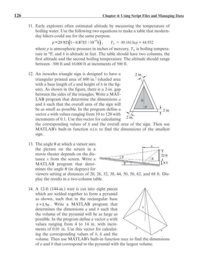
126 Chapter 4: Using Script Files and Managing Data
11. Early explorers often estimated altitude by measuring the temperature ofboiling water. Use the following two equations to make a table that modern-day hikers could use for the same purpose.
,
where p is atmospheric pressure in inches of mercury, is boiling tempera-ture in °F, and h is altitude in feet. The table should have two columns, thefirst altitude and the second boiling temperature. The altitude should rangebetween –500 ft and 10,000 ft at increments of 500 ft.
12. An isosceles triangle sign is designed to have atriangular printed area of 600 in.2 (shaded areawith a base length of a and height of h in the fig-ure). As shown in the figure, there is a 2-in. gapbetween the sides of the triangles. Write a MAT-LAB program that determine the dimensions aand h such that the overall area of the sign willbe as small as possible. In the program define avector a with values ranging from 10 to 120 withincrements of 0.1. Use this vector for calculatingthe corresponding values of h and the overall area of the sign. Then useMATLAB’s built-in function min to find the dimensions of the smallestsign.
13. The angle at which a viewer seesthe picture on the screen in amovie theater depends on the dis-tance x from the screen. Write aMATLAB program that deter-mines the angle (in degrees) forviewers setting at distances of 20, 26, 32, 38, 44, 50, 56, 62, and 68 ft. Dis-play the results in a two-column table.
14. A 12-ft (144-in.) wire is cut into eight pieceswhich are welded together to form a pyramidas shown, such that in the rectangular base
. Write a MATLAB program thatdetermines the dimensions a and b such thatthe volume of the pyramid will be as large aspossible. In the program define a vector a withvalues ranging from 4 to 14 in. with incre-ments of 0.01 in. Use this vector for calculat-ing the corresponding values of b, h and thevolume. Then use MATLAB’s built-in function max to find the dimensionsof a and b that correspond to the pyramid with the largest volume.
Tb 49.161 pln 44.932+=
Tb
2 in.a
h
2 in.
2 in.
ab
h

4.7 Problems 127
15. A person at point A spots a child introuble at point B across the river. Theperson can run at a speed of 8.6 ft/s andcan swim at a speed of 3.9 ft/s. In orderto reach the child in the shortest time theperson runs to point C and then swimsto point B, as shown. Write a MATLAB program that determines thedistance x to point C that minimizes the time the person can reach the child.In the program define a vector x with values ranging from 0 to 5,000 withincrements of 1. Use this vector to calculate the corresponding values ofx.Then use MATLAB’s built-in function min to find the value of x thatcorresponds to the shortest time.
16. The maximum stress max at the edgeof a hole (diameter d) in a thin plate,with width w and thickness t, loadedby a tensile force F as shown is givenby:
where and .
Write a program in a script file that calculates max. The program shouldread the values of F, w, d, and t from an ASCII text file using the load com-mand. The output should be in the form of a paragraph combining text andnumbers— i.e., something like: “The maximum stress in a plate with a widthof XX in. and thickness of XX in. and a hole of XX in. in diameter, due to atensile force of XXX lb is XXXX psi, where XX stands for numerical val-ues.” The stress should be rounded to the nearest integer. Use the programto calculate max when in., in., in., and
lb.
17. The airplane shown is flying at a constantspeed of mi/h along a straight path asshown. The airplane is being tracked by aradar station positioned a distance ftbelow point A. The airplane is at point A at
. Write a MATLAB program that calcu-lates and r as functions of time for
s. Display the results in athree-column table where the first column is t, the second is the angle indegrees, and the third is the corresponding value of r.
A
B
C
10,000 ft
x
3,000 ft
FFd w
t

128 Chapter 4: Using Script Files and Managing Data
18. The intrinsic electrical conductivity of a semiconductor can be approxi-mated by:
where is measured in , is the band gap energy, k is Boltz-
mann’s constant ( eV/K), and T is temperature in kelvins. Forgermanium, and eV. Write a program in a script file
that calculates the intrinsic electrical conductivity for germanium for vari-ous temperatures. The values of the temperature should be read from an xlsspreadsheet using the xlsread command. The output should be presentedas a table where the first column is the temperature and the second columnis the intrinsic electrical conductivity. Use the following values for tempera-ture: 400, 435, 475, 500, 520, and 545 K.
19. The pressure drop p in pascals (Pa) for afluid flowing in a pipe with a suddenincrease in diameter is given by:
where is the density of the fluid, v, the velocity of the flow, and d and D aredefined in the figure. Write a program in a script file that calculates the pres-sure drop p. When the script file is executed, it requests the user to input
the density in kg/m3, the velocity in m/s, and values of the nondimensionalratio as a vector. The program displays the inputted values of and vfollowed by a table with the values of in the first column and the cor-responding values of p in the second column.
Execute the program assuming flow of gasoline ( kg/m3) atm/s and the following ratios of diameters
.
20. The net heat exchange by radiation from plate 1with radius b to plate 2 with radius a that areseparated by a distance c is given by:
where and are the absolute temperatures
of the plates, W/(m2-K4) is theStefan-Boltzmann constant, and is ashape factor which, for the arrangement in thefigure, is given by:
Eg
C 13.83= Eg 0.67=
Ddv
737=
v 5=
a
b
c
T1 T2

4.7 Problems 129
where , , and . Write a script file that cal-culates the heat exchange q. For input the program asks the user to entervalues for , , a, b, and c. For output the program prints a summary ofthe geometry and temperatures and then prints the value of q. Use the scriptto calculate the results for K, K, m, m, and
, 1, and 10 m.
21. The equation of a circle in a plane with radius R and a center at point is given by:
The equation can also be written in the form:
where Given the coordinates of three points , , and it is
possible to determine the radius and the coordinates of the center of the cir-cle that passes through the three points. This is done by substituting thecoordinate of each of the points in the equation and solving the system ofthree linear equations for , , and c.
Write a program in a script file that calculates the coordinates of thecenter and the radius of a circle that passes through three given points.When executed the program asks the user to enter the coordinates of thethree points. The program then calculates the center and radius and displaysthe results in the following format: “The coordinates of the center are (xx.x,xx.x) and the radius is xx.x.”, where xx.x stands for the calculated quantitiesrounded to the nearest tenth. Execute the program entering the followingthree points: (11.5, 5), (3.2, 8.6), and (–4.5, –6.8).
22. A truss is a structure made of mem-bers joined at their ends. For the trussshown in the figure, the forces in the11 members are determined by solvingthe following system of 11 equations:
, ,
, , ,
, , ,
,
Write the equations in matrix form and use MATLAB to determine theforces in the members. A positive force means tensile force and a negativeforce means compressive force. Display the results in a table where the firstcolumn displays the member number and the second column displays thecorresponding force.
T1 T2
T1 400= T2 600= a 1= b 2=c 0.1=
800 lb
23
4
5
6
7
8
9
400 lb1200 lb
136 ft
48 ft42 ft30 ft
10
11

130 Chapter 4: Using Script Files and Managing Data
23. A truss is a structure made of mem-bers joined at their ends. For thetruss shown in the figure, the forcesin the seven members are deter-mined by solving the following sys-tem of seven equations.
, ,
,
, Write the equations in matrix form and use MATLAB to determine theforces in the members. A positive force means tensile force and a negativeforce means compressive force. Display the results in a table where the firstcolumn displays the member number and the second column displays thecorresponding force.
24. The graph of the function passes through the points(–1.2, 18.8), (0.2, 5), (2, 16), and (3.5, 15). Determine the constants a, b, c, andd. (Write a system of four equations with four unknowns, and use MAT-LAB to solve the equations.)
25. The graph of the function passes through thepoints (–2.5, –62), (–1.5, –7.2), (–0.5, 8.3), (1, 3.7), and (3, 45.7). Determine theconstants a, b, c, d, and e. (Write a system of five equations with fourunknowns, and use MATLAB to solve the equations.)
26. The surface of many airfoils can bedescribed with an equation of the form
where t is the maximum thickness as a fraction of the chord length c (e.g.,
). Given that m and m, the following values for yhave been measured for a particular airfoil:
Determine the constants , and . (Write a system of five equa-tions and five unknowns, and use MATLAB to solve the equations.)
x (m) 0.15 0.35 0.5 0.7 0.85
y (m) 0.08909 0.09914 0.08823 0.06107 0.03421
3000 lb
2
3
4
56
7
6000 N8000 N
1
16 m16 m16 m
13 m
tmax ct= c 1= t 0.2=
a0 a1 a2 a3, , , a4

4.7 Problems 131
27. During a golf match, a certain number of points are awarded for each eagleand a different number for each birdie. No points are awarded for par, anda certain number of points are deducted for each bogey and a differentnumber deducted for each double bogey (or worse). The newspaper reportof an important match neglected to mention what these point values were,but did provide the following table of the results:
From the information in the table write four equations in terms of fourunknowns. Solve the equations for the unknown points awarded for eaglesand birdies and points deducted for bogeys and double bogeys.
28. The dissolution of copper sulfide in aqueous nitric acid is described by thefollowing chemical equation:
where the coefficients a, b, c, d, e, f, and g are the numbers of the variousmolecules participating in the reaction and are unknown. The unknowncoefficients are determined by balancing each atom on left and right andthen balancing the ionic charge. The resulting equations are:
, , , , , There are seven unknowns and only six equations. A solution can still beobtained, however, by taking advantage of the fact that all the coefficientsmust be positive integers. Add a seventh equation by guessing andsolve the system of equations. The solution is valid if all the coefficients arepositive integers. If this is not the case, take and repeat the solution.Continue the process until all the coefficients in the solution are positiveintegers.
29. The heat index HI, calculated from the air temperature and relative humid-ity, is the apparent temperature felt by the body. An equation used by theNational Weather Service for calculating the HI is given by:
where T is the temperature in °F, and R is the relative humidity in integerpercentage. Write a MATLAB program in a script file that displays the fol-lowing chart of heat index for given air temperature and relative humidity in
Golfer Eagles Birdies Pars Bogeys Doubles Points
A 1 2 10 1 1 5
B 2 3 11 0 1 12
C 1 4 10 1 0 11
D 1 3 10 2 0 8
a d= a e= b f= 3b 4e f g+ += c 2g=
a 1=
a 2=

132 Chapter 4: Using Script Files and Managing Data
the Command Window: Temperature (F)
80 82 84 86 88 90 92 94 Relative
Humidity
(%)
50 81 83 85 88 91 95 99 103
55 81 84 86 89 93 97 101 106
60 82 84 88 91 95 100 105 110
65 82 85 89 93 98 103 108 114
70 83 86 90 95 100 106 112 119
75 84 88 92 97 103 109 116 124
30. The stress intensity factor K at a crack is given by
where is the far-field stress, a is the crack
length, and C is a parameter that depends on the geome-try of the specimen and crack. For the case of the edgecrack shown in the figure, C is given by:
Write a script file that will print out a table of values withthe ratio a/b in the first column and the correspondingparameter C in the second column. Let a/b rangebetween 0.05 and 0.80 with increments of 0.05.

133
Chapter 5 Two-Dimensional Plots
Plots are a very useful tool for presenting information. This is true in any field,but especially in science and engineering, where MATLAB is mostly used.MATLAB has many commands that can be used for creating different types ofplots. These include standard plots with linear axes, plots with logarithmic andsemi-logarithmic axes, bar and stairs plots, polar plots, three-dimensional con-tour surface and mesh plots, and many more. The plots can be formatted tohave a desired appearance. The line type (solid, dashed, etc.), color, and thick-ness can be prescribed, line markers and grid lines can be added, as can titlesand text comments. Several graphs can be created in the same plot, and severalplots can be placed on the same page. When a plot contains several graphs and/or data points, a legend can be added to the plot as well.
This chapter describes how MATLAB can be used to create and formatmany types of two-dimensional plots. Three-dimensional plots are addressedseparately in Chapter 9. An example of a simple two-dimensional plot that wascreated with MATLAB is shown in Figure 5-1. The figure contains two curvesthat show the variation of light intensity with distance. One curve is constructedfrom data points measured in an experiment, and the other curve shows thevariation of light as predicted by a theoretical model. The axes in the figure areboth linear, and different types of lines (one solid and one dashed) are used forthe curves. The theoretical curve is shown with a solid line, while the experimen-tal points are connected with a dashed line. Each data point is marked with acircular marker. The dashed line that connects the experimental points is actu-ally red when the plot is displayed in the Figure Window. As shown, the plot inFigure 5-1 is formatted to have a title, axis titles, a legend, markers, and a boxedtext label.

134 Chapter 5: Two-Dimensional Plots
5.1 THE plot COMMAND
The plot command is used to create two-dimensional plots. The simplest formof the command is:
The arguments x and y are each a vector (one-dimensional array). The two vec-tors must have the same number of elements. When the plot command is exe-cuted, a figure is created in the Figure Window. If not already open, the FigureWindow opens automatically when the command is executed. The figure has asingle curve with the x values on the abscissa (horizontal axis) and the y valueson the ordinate (vertical axis). The curve is constructed of straight-line segmentsthat connect the points whose coordinates are defined by the elements of thevectors x and y. Each of the vectors, of course, can have any name. The vectorthat is typed first in the plot command is used for the horizontal axis, and thevector that is typed second is used for the vertical axis. If only one vector isentered as an input argument in the plot command (for example plot(y))than the figure will show a plot of the values of the elements of the vector( ) versus the element number ( ).
The figure that is created has axes with a linear scale and default range. Forexample, if a vector x has the elements 1, 2, 3, 5, 7, 7.5, 8, 10, and a vector y has
Figure 5-1: Example of a formatted two-dimensional plot.
DISTANCE (cm)8 10 12 14 16 18 20 22 24
INT
EN
SIT
Y (
lux)
0
200
400
600
800
1000
1200
Comparison between theory and experiment.
Light Intensity as a Function of Distance
TheoryExperiment
X AXIS LABEL
LEGEND
TEXTLABEL
PLOT TITLE
Y AXIS LABEL
MARKER
plot(x,y)
Vector Vector
y 1 y 2 y 3, , , 1 2 3, , ,

5.1 The plot Command 135
the elements 2, 6.5, 7, 7, 5.5, 4, 6, 8, a simple plot of y versus x can be created bytyping the following in the Command Window:
Once the plot command is executed, the Figure Window opens and the plot isdisplayed, as shown in Figure 5-2.
The plot appears on the screen in blue, which is the default line color.The plot command has additional, optional arguments that can be used to
specify the color and style of the line and the color and type of markers, if anyare desired. With these options the command has the form:
Line Specifiers:
Line specifiers are optional and can be used to define the style and color of theline and the type of markers (if markers are desired). The line style specifiers are:
>> x=[1.1 1.8 3.2 5.5 7 7.5 8 10];
>> y=[2 6.5 7 7 5.5 4 6 8];
>> plot(x,y)
Figure 5-2: The Figure Window with a simple plot.
Line Style Specifier Line Style Specifier
solid (default) - dotted :
dashed -- dash-dot -.
plot(x,y,‘line specifiers’,‘PropertyName’,PropertyValue)
(Optional) Specifiers thatdefine the type and colorof the line and markers.
Vector Vector(Optional) Properties withvalues that can be used tospecify the line width, anda marker’s size and edge,and fill colors.
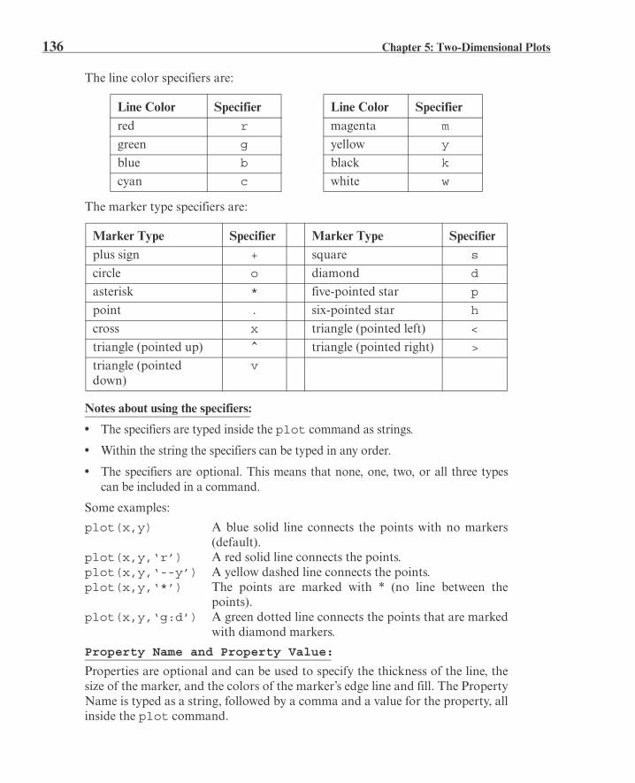
136 Chapter 5: Two-Dimensional Plots
The line color specifiers are:
The marker type specifiers are:
Notes about using the specifiers:
• The specifiers are typed inside the plot command as strings.
• Within the string the specifiers can be typed in any order.
• The specifiers are optional. This means that none, one, two, or all three typescan be included in a command.
Some examples:
plot(x,y) A blue solid line connects the points with no markers(default).
plot(x,y,‘r’) A red solid line connects the points.plot(x,y,‘--y’) A yellow dashed line connects the points.plot(x,y,‘*’) The points are marked with * (no line between the
points).plot(x,y,‘g:d’) A green dotted line connects the points that are marked
with diamond markers.
Property Name and Property Value:
Properties are optional and can be used to specify the thickness of the line, thesize of the marker, and the colors of the marker’s edge line and fill. The PropertyName is typed as a string, followed by a comma and a value for the property, allinside the plot command.
Line Color Specifier Line Color Specifierred r magenta m
green g yellow y
blue b black k
cyan c white w
Marker Type Specifier Marker Type Specifierplus sign + square s
circle o diamond d
asterisk * five-pointed star p
point . six-pointed star h
cross x triangle (pointed left) <
triangle (pointed up) ^ triangle (pointed right) >
triangle (pointed down)
v

5.1 The plot Command 137
Four properties and their possible values are:
For example, the command
plot(x,y,‘-mo’,‘LineWidth’,2,‘markersize’,12, ‘MarkerEdgeColor’,‘g’,‘markerfacecolor’,‘y’)
creates a plot that connects the points with a magenta solid line and circles asmarkers at the points. The line width is 2 points and the size of the circle mark-ers is 12 points. The markers have a green edge line and yellow filling.
A note about line specifiers and properties:
The three line specifiers, which indicate the style and color of the line, and thetype of the marker can also be assigned with a PropertyName argument fol-lowed by a PropertyValue argument. The Property Names for the line speci-fiers are:
As with any command, the plot command can be typed in the CommandWindow, or it can be included in a script file. It also can be used in a functionfile (explained in Chapter 7). It should also be remembered that before the plotcommand can be executed, the vectors x and y must have assigned elements.
Property name Description Possible property values
LineWidth(or linewidth)
Specifies the width of theline.
A number in units ofpoints (default 0.5).
MarkerSize(or markersize)
Specifies the size of themarker.
A number in units ofpoints.
MarkerEdgeColor(or markeredgecolor)
Specifies the color of themarker, or the color ofthe edge line for filledmarkers.
Color specifiers fromthe table above, typedas a string.
MarkerFaceColor(or markerfacecolor)
Specifies the color of thefilling for filled markers.
Color specifiers fromthe table above, typedas a string.
Specifier Property Name Possible property values
Line style linestyle (or LineStyle)
Line style specifier from the table above, typed as a string.
Line color color (or Color) Color specifier from the table above, typed as a string.
Marker marker (or Marker) Marker specifier from the table above, typed as a string.

138 Chapter 5: Two-Dimensional Plots
This can be done, as was explained in Chapter 2, by entering values directly, byusing commands, or as the result of mathematical operations. The next two sub-sections show examples of creating simple plots.
5.1.1 Plot of Given Data
In this case given data is used to create vectors that are then used in the plotcommand. The following table contains sales data of a company from 1988 to1994.
To plot this data, the list of years is assigned to one vector (named yr), andthe corresponding sales data is assigned to a second vector (named sle). TheCommand Window where the vectors are created and the plot command isused is shown below:
Once the plot command is executed, the Figure Window with the plot, asshown in Figure 5-3, opens. The plot appears on the screen in red.
Year 1988 1989 1990 1991 1992 1993 1994
Sales (millions)
8 12 20 22 18 24 27
>> yr=[1988:1:1994];
>> sle=[8 12 20 22 18 24 27];
>> plot(yr,sle,'--r*','linewidth',2,'markersize',12)
>>
Figure 5-3: The Figure Window with a plot of the sales data.
Line Specifiers:dashed red line and asterisk marker.
Property Name and Property Value:the line width is 2 points and the marker size is 12 points.

5.1 The plot Command 139
5.1.2 Plot of a Function
In many situations there is a need to plot a given function. This can be done inMATLAB by using the plot or the fplot command. The use of the plotcommand is explained below. The fplot command is explained in detail in thenext section.
In order to plot a function with the plot command, the userneeds to first create a vector of values of x for the domain over which the func-tion will be plotted. Then a vector y is created with the corresponding values of
by using element-by-element calculations (see Chapter 3). Once the twovectors are defined, they can be used in the plot command.
As an example, the plot command is used to plot the function
for . A program that plots this function is shown inthe following script file.
Once the script file is executed, the plot is created in the Figure Window, asshown in Figure 5-4. Since the plot is made up of segments of straight lines thatconnect the points, to obtain an accurate plot of a function, the spacing betweenthe elements of the vector x must be appropriate. Smaller spacing is needed for a
% A script file that creates a plot of
% the function: 3.5.^(-0.5*x).*cos(6x)
x=[-2:0.01:4];
y=3.5.^(-0.5*x).*cos(6*x);
plot(x,y)
Figure 5-4: The Figure Window with a plot of the function .
y f x=
f x
Create vector x with the domain of the function.
Create vector y with the func-tion value at each x.
Plot y as a function of x.
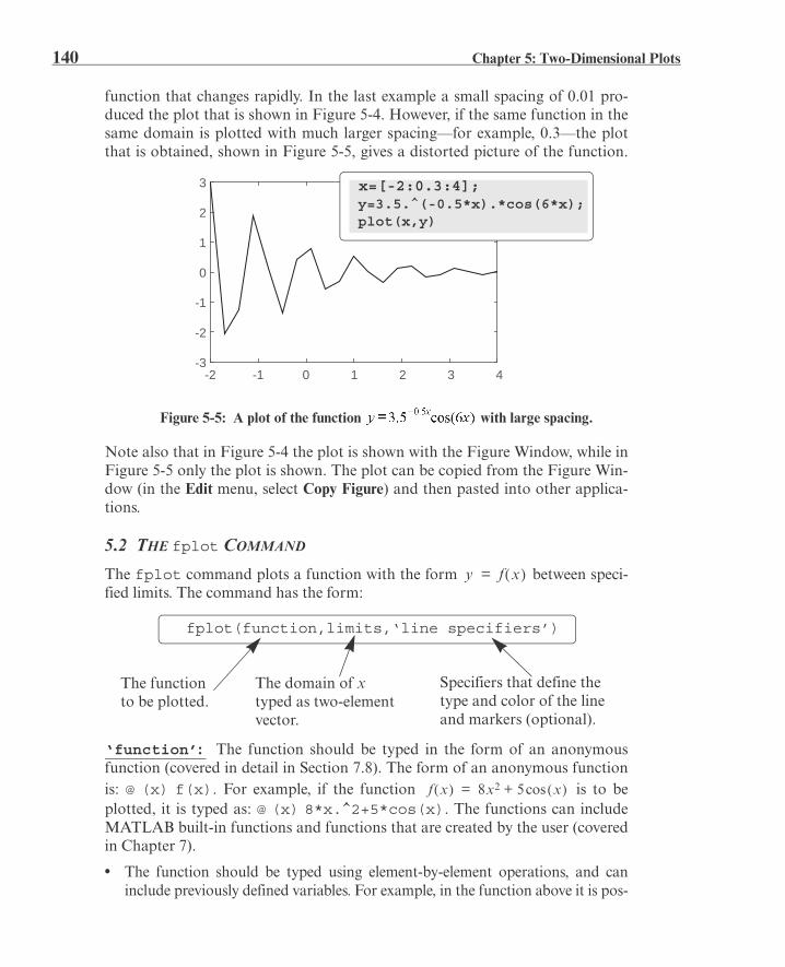
140 Chapter 5: Two-Dimensional Plots
function that changes rapidly. In the last example a small spacing of 0.01 pro-duced the plot that is shown in Figure 5-4. However, if the same function in thesame domain is plotted with much larger spacing—for example, 0.3—the plotthat is obtained, shown in Figure 5-5, gives a distorted picture of the function.
Note also that in Figure 5-4 the plot is shown with the Figure Window, while inFigure 5-5 only the plot is shown. The plot can be copied from the Figure Win-dow (in the Edit menu, select Copy Figure) and then pasted into other applica-tions.
5.2 THE fplot COMMAND
The fplot command plots a function with the form between speci-fied limits. The command has the form:
‘function’: The function should be typed in the form of an anonymousfunction (covered in detail in Section 7.8). The form of an anonymous functionis: @ (x) f(x). For example, if the function is to beplotted, it is typed as: @ (x) 8*x.^2+5*cos(x). The functions can includeMATLAB built-in functions and functions that are created by the user (coveredin Chapter 7).
• The function should be typed using element-by-element operations, and caninclude previously defined variables. For example, in the function above it is pos-
Figure 5-5: A plot of the function with large spacing.
-2 -1 0 1 2 3 4-3
-2
-1
0
1
2
3 x=[-2:0.3:4]; y=3.5.^(-0.5*x).*cos(6*x); plot(x,y)
y f x=
fplot(function,limits,‘line specifiers’)
Specifiers that define the type and color of the line and markers (optional).
The function to be plotted.
The domain of x typed as two-element vector.
f x 8x2 5 xcos+=

5.3 Plotting Multiple Graphs in the Same Plot 141
sible to assign 8 to a variable, and then use the variable when the function istyped in the fplot command.
• The function to be plotted can be typed as a function of any letter. For example,the function in the previous paragraph can be typed as @ (t)8*t.^2+5*cos(t) or @ (z) 8*z.^2+5*cos(z)’.
limits: The limits argument is a vector with two elements that specify thedomain of x [xmin,xmax], or a vector with four elements that specifies thedomain of x and the limits of the y-axis [xmin,xmax,ymin,ymax].
line specifiers: The line specifiers are the same as in the plot com-mand. For example, a plot of the function for canbe created with the fplot command by typing:
in the Command Window. The figure that is obtained in the Figure Window isshown in Figure 5-6.
5.3 PLOTTING MULTIPLE GRAPHS IN THE SAME PLOT
In many situations, there is a need to make several graphs in the same plot. Thisis shown, for example, in Figure 5-1 where two graphs are plotted in the samefigure. There are three methods to plot multiple graphs in one figure. One is byusing the plot command, the second is by using the hold on and hold offcommands, and the third is by using the line command.
5.3.1 Using the plot Command
Two or more graphs can be created in the same plot by typing pairs of vectorsinside the plot command. The command
plot(x,y,u,v,t,h)
creates three graphs—y vs. x, v vs. u, and h vs. t—all in the same plot. The vec-tors of each pair must be of the same length. MATLAB automatically plots thegraphs in different colors so that they can be identified. It is also possible to add
>> fplot(@ (x) x.^2+4*sin(2*x)-1,[-3 3])
Figure 5-6: A plot of the function .
-3 -2 -1 0 1 2 3-4
-2
0
2
4
6
8
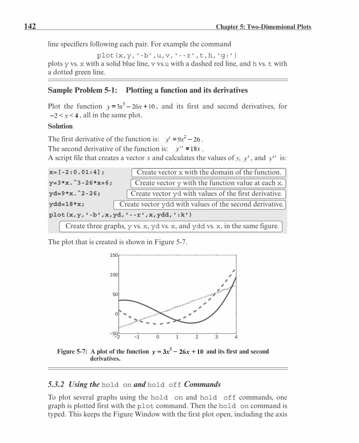
142 Chapter 5: Two-Dimensional Plots
line specifiers following each pair. For example the command
plot(x,y,‘-b’,u,v,‘--r’,t,h,‘g:’)plots y vs. x with a solid blue line, v vs.u with a dashed red line, and h vs. t witha dotted green line.
Sample Problem 5-1: Plotting a function and its derivatives
Plot the function , and its first and second derivatives, for, all in the same plot.
Solution
The first derivative of the function is: .The second derivative of the function is: .A script file that creates a vector x and calculates the values of y, , and is:
The plot that is created is shown in Figure 5-7.
5.3.2 Using the hold on and hold off Commands
To plot several graphs using the hold on and hold off commands, onegraph is plotted first with the plot command. Then the hold on command istyped. This keeps the Figure Window with the first plot open, including the axis
x=[-2:0.01:4];
y=3*x.^3-26*x+6;
yd=9*x.^2-26;
ydd=18*x;
plot(x,y,'-b',x,yd,'--r',x,ydd,':k')
Figure 5-7: A plot of the function and its first and second derivatives.
Create vector x with the domain of the function.
Create vector y with the function value at each x.
Create vector yd with values of the first derivative.
Create vector ydd with values of the second derivative.
Create three graphs, y vs. x, yd vs. x, and ydd vs. x, in the same figure.
−2 −1 0 1 2 3 4−50
0
50
100
150

5.3 Plotting Multiple Graphs in the Same Plot 143
properties and formatting (see Section 5.4) if any was done. Additional graphscan be added with plot commands that are typed next. Each plot commandcreates a graph that is added to that figure. The hold off command stops thisprocess. It returns MATLAB to the default mode, in which the plot commanderases the previous plot and resets the axis properties.
As an example, a solution of Sample Problem 5-1 using the hold on andhold off commands is shown in the following script file:
5.3.3 Using the line Command
With the line command additional graphs (lines) can be added to a plot thatalready exists. The form of the line command is:
The format of the line command is almost the same as the plot command(see Section 5.1). The line command does not have the line specifiers, but theline style, color, and marker can be specified with the Property Name and prop-erty value features. The properties are optional, and if none are entered MAT-LAB uses default properties and values. For example, the command:
line(x,y,‘linestyle’,‘--’,‘color’,‘r’,‘marker’,‘o’)
will add a dashed red line with circular markers to a plot that already exists.The major difference between the plot and line commands is that the
plot command starts a new plot every time it is executed, while the line com-mand adds lines to a plot that already exists. To make a plot that has severalgraphs, a plot command is typed first and then line commands are typed foradditional graphs. (If a line command is entered before a plot command, anerror message is displayed.)
x=[-2:0.01:4];
y=3*x.^3-26*x+6;
yd=9*x.^2-26;
ydd=18*x;
plot(x,y,'-b')
hold on
plot(x,yd,'--r')
plot(x,ydd,':k')
hold off
The first graph is created.
Two more graphs are added to the figure.
line(x,y,‘PropertyName’,PropertyValue)
(Optional) Properties with values that can beused to specify the line style, color, and width,marker type, size, and edge and fill colors.
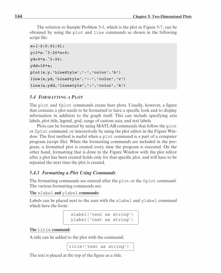
144 Chapter 5: Two-Dimensional Plots
The solution to Sample Problem 5-1, which is the plot in Figure 5-7, can beobtained by using the plot and line commands as shown in the followingscript file:
5.4 FORMATTING A PLOT
The plot and fplot commands create bare plots. Usually, however, a figurethat contains a plot needs to be formatted to have a specific look and to displayinformation in addition to the graph itself. This can include specifying axislabels, plot title, legend, grid, range of custom axis, and text labels.
Plots can be formatted by using MATLAB commands that follow the plotor fplot command, or interactively by using the plot editor in the Figure Win-dow. The first method is useful when a plot command is a part of a computerprogram (script file). When the formatting commands are included in the pro-gram, a formatted plot is created every time the program is executed. On theother hand, formatting that is done in the Figure Window with the plot editorafter a plot has been created holds only for that specific plot, and will have to berepeated the next time the plot is created.
5.4.1 Formatting a Plot Using Commands
The formatting commands are entered after the plot or the fplot command.The various formatting commands are:
The xlabel and ylabel commands:
Labels can be placed next to the axes with the xlabel and ylabel commandwhich have the form:
The title command:
A title can be added to the plot with the command:
The text is placed at the top of the figure as a title.
x=[-2:0.01:4];
y=3*x.^3-26*x+6;
yd=9*x.^2-26;
ydd=18*x;
plot(x,y,'LineStyle','-','color','b')
line(x,yd,'LineStyle','--','color','r')
line(x,ydd,'linestyle',':','color','k')
xlabel(‘text as string’)ylabel(‘text as string’)
title(‘text as string’)

5.4 Formatting a Plot 145
The text command:
A text label can be placed in the plot with the text or gtext commands:
The text command places the text in the figure such that the first character ispositioned at the point with the coordinates x, y (according to the axes of thefigure). The gtext command places the text at a position specified by the user.When the command is executed, the Figure Window opens and the user speci-fies the position with the mouse.
The legend command:
The legend command places a legend on the plot. The legend shows a sampleof the line type of each graph that is plotted, and places a label, specified by theuser, beside the line sample. The form of the command is:
legend(‘string1’,‘string2’, ..... ,‘Location’,‘pos’)
The strings are the labels that are placed next to the line sample. Their order cor-responds to the order in which the graphs were created. The ‘Loca-tion’,‘pos’ are optional strings that specifies where in the figure the legendis to be placed. Several options are:
NE Places the legend at the upper-right corner of the plot (default).NW Places the legend at the upper-left corner of the plot.SE Places the legend at the lower-right corner of the plot.SW Places the legend at the lower-left corner of the plot.B Places the legend inside the plot in a location that interferes the least with
the graphs.BO Places the legend in a least unused space outside the plot.
To read about other options for the position of the legend type help legendin the Command Window.
Formatting the text within the xlabel, ylabel, title, text
and legend commands:
The text in the string that is included in the command and is displayed when thecommand is executed can be formatted. The formatting can be used to definethe font, size, position (superscript, subscript), style (italic, bold, etc.), and colorof the characters, the color of the background, and many other details of thedisplay. Some of the more common formatting possibilities are described below.A complete explanation of all the formatting features can be found in the HelpWindow under Text and Text Properties. The formatting can be done either byadding modifiers inside the string, or by adding to the command optionalPropertyName and PropertyValue arguments following the string.
text(x,y,‘text as string’)gtext(‘text as string’)

146 Chapter 5: Two-Dimensional Plots
The modifiers are characters that are inserted within the string. Some of themodifiers that can be added are:
These modifiers affect the text from the point at which they are inserted until theend of the string. It is also possible to have the modifiers applied to only a sec-tion of the string by typing the modifier and the text to be affected inside braces{ }.
Subscript and superscript:
A single character can be displayed as a subscript or a superscript by typing _(the underscore character) or ^ in front of the character, respectively. Severalconsecutive characters can be displayed as a subscript or a superscript by typingthe characters inside braces { } following the _ or the ^.
Greek characters:
Greek characters can be included in the text by typing \name of the letterwithin the string. To display a lowercase Greek letter, the name of the lettershould be typed in all lowercase English characters. To display a capital Greekletter, the name of the letter should start with a capital letter. Some examplesare:
Formatting of the text that is displayed by the xlabel, ylabel, title,and text commands can also be done by adding optional PropertyNameand PropertyValue arguments following the string inside the command.
Modifier Effect Modifier Effect
\bf bold font \fontname{fontname} specified font is used
\it italic style \fontsize{fontsize} specified font size is used
\rm normal font
Characters in the string
Greekletter
Characters in the string
Greekletter
\alpha \Phi
\beta \Delta
\gamma \Gamma
\theta \Lambda
\pi \Omega
\sigma \Sigma

5.4 Formatting a Plot 147
With this option, the text command, for example, has the form:
In the other three commands the PropertyName and PropertyValue argu-ments are added in the same way. The PropertyName is typed as a string, andthe PropertyValue is typed as a number if the property value is a numberand as a string if the property value is a word or a letter character. Some of theProperty Names and corresponding possible Property Values are:
The axis command:
When the plot(x,y) command is executed, MATLAB creates axes with lim-its that are based on the minimum and maximum values of the elements of xand y. The axis command can be used to change the range and the appearanceof the axes. In many situations, a graph looks better if the range of the axesextend beyond the range of the data. The following are some of the possibleforms of the axis command:
Property name Description Possible property values
Rotation Specifies the orientationof the text.
Scalar (degrees)Default: 0
FontAngle Specifies italic or nor-mal style characters.
normal, italicDefault: normal
FontName Specifies the font for thetext.
Font name that is available in the sys-tem.
FontSize Specifies the size of thefont.
Scalar (points)Default: 10
FontWeight Specifies the weight ofthe characters.
light, normal, boldDefault: normal
Color Specifies the color of thetext.
Color specifiers (see Section 5.1).
Background-Color
Specifies the back-ground color (rectangu-lar area).
Color specifiers (see Section 5.1).
EdgeColor Specifies the color of theedge of a rectangular boxaround the text.
Color specifiers (see Section 5.1).Default: none.
LineWidth Specifies the width of theedge of a rectangular boxaround the text.
Scalar (points)Default: 0.5
text(x,y,‘text as string’,PropertyName,PropertyValue)
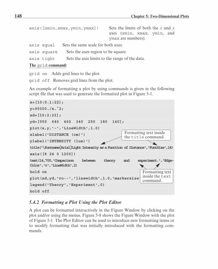
148 Chapter 5: Two-Dimensional Plots
axis([xmin,xmax,ymin,ymax]) Sets the limits of both the x and yaxes (xmin, xmax, ymin, andymax are numbers).
axis equal Sets the same scale for both axes.
axis square Sets the axes region to be square.
axis tight Sets the axis limits to the range of the data.
The grid command:
grid on Adds grid lines to the plot.
grid off Removes grid lines from the plot.
An example of formatting a plot by using commands is given in the followingscript file that was used to generate the formatted plot in Figure 5-1.
5.4.2 Formatting a Plot Using the Plot Editor
A plot can be formatted interactively in the Figure Window by clicking on theplot and/or using the menus. Figure 5-8 shows the Figure Window with the plotof Figure 5-1. The Plot Editor can be used to introduce new formatting items orto modify formatting that was initially introduced with the formatting com-mands.
x=[10:0.1:22];
y=95000./x.^2;
xd=[10:2:22];
yd=[950 640 460 340 250 180 140];
plot(x,y,'-','LineWidth',1.0)
xlabel('DISTANCE (cm)')
ylabel('INTENSITY (lux)')
title('\fontname{Arial}Light Intensity as a Function of Distance','FontSize',14)
axis([8 24 0 1200])
text(14,700,'Comparison between theory and experiment.','Edge-Color','r','LineWidth',2)
hold on
plot(xd,yd,'ro--','linewidth',1.0,'markersize',10)
legend('Theory','Experiment',0)
hold off
Formatting text inside the title command.
Formatting text inside the text command.

5.5 Plots with Logarithmic Axes 149
5.5 PLOTS WITH LOGARITHMIC AXES
Many science and engineering applications require plots in which one or bothaxes have a logarithmic (log) scale. Log scales provide means for presenting dataover a wide range of values. It also provides a tool for identifying characteristicsof data and possible forms of mathematical relationships that can be appropri-ate for modeling the data (see Section 8.2.2).
MATLAB commands for making plots with log axes are:
semilogy(x,y) Plots y versus x with a log (base 10) scale for the y axis and linear scale for the x axis.
semilogx(x,y) Plots y versus x with a log (base 10) scale for the x axis and linear scale for the y axis.
loglog(x,y) Plots y versus x with a log (base 10) scale for both axes.
Line specifiers and Property Name and Property Value arguments can be addedto the commands (optional) just as in the plot command. As an example, Fig-
ure 5-9 shows a plot of the function for . The figureshows four plots of the same function: one with linear axes, one with a log scalefor the y axis, one with a log scale for the x axis, and one with a log scale on bothaxes.
Figure 5-8: Formatting a plot using the Plot Editor.
Click the arrow button to start the plot edit mode. Then clickon an item. A window with formatting tool for the item opens.
Use the Edit and Insert menus to add formatting objects, or to edit existing objects.
Change posi-tion of a label, legend, or other object by clicking on the object and dragging.

150 Chapter 5: Two-Dimensional Plots
Notes for plots with logarithmic axes:
• The number zero cannot be plotted on a log scale (since a log of zero is notdefined).
• Negative numbers cannot be plotted on log scales (since a log of a negative num-ber is not defined).
5.6 PLOTS WITH ERROR BARS
Experimental data that is measured and then displayed in plots frequently con-tains error and scatter. Even data that is generated by computational modelsincludes error or uncertainty that depends on the accuracy of the input parame-ters and the assumptions in the mathematical models that are used. One methodof plotting data that displays the error, or uncertainty, is by using error bars. Anerror bar is typically a short vertical line that is attached to a data point in aplot. It shows the magnitude of the error that is associated with the value that isdisplayed by the data point. For example, Figure 5-10 shows a plot with errorbars for the experimental data from Figure 5-1.
Figure 5-9: Plots of with linear, semilog, and log-log scales.
x=linspace(0.1,60,1000);y=2.^(-0.2*x+10);plot(x,y)
Linear
x=linspace(0.1,60,1000);y=2.^(-0.2*x+10);semilogx(x,y)
x=linspace(0.1,60,1000);y=2.^(-0.2*x+10);loglog(x,y)
x=linspace(0.1,60,1000);y=2.^(-0.2*x+10);semilogy(x,y)
Linear
Log
Lin
ear
Lin
ear
Log
Log
Log

5.6 Plots with Error Bars 151
Plots with error bars can be done in MATLAB with the errorbar com-mand. Two forms of the command, one for making plots with symmetric errorbars (with respect to the value of the data point) and the other for nonsymmet-ric error bars at each point, are presented. When the error is symmetric, theerror bar extends the same length above and below the data point, and the com-mand has the form:
• The lengths of the three vectors x, y, and e must be the same.
• The length of the error bar is twice the value of e. At each point the error barextends from y(i)-e(i) to y(i)+e(i).
The plot in Figure 5-10, which has symmetric error bars, was done by exe-cuting the following code:
The command for making a plot with error bars that are not symmetric is:
Figure 5-10: A plot with error bars.
xd=[10:2:22];
yd=[950 640 460 340 250 180 140];
ydErr=[30 20 18 35 20 30 10]
errorbar(xd,yd,ydErr)
xlabel('DISTANCE (cm)')ylabel('INTENSITY (lux)')
8 10 12 14 16 18 20 22 24100
200
300
400
500
600
700
800
900
1000
DISTANCE (cm)
INT
EN
SIT
Y (
lux)
errorbar(x,y,e)
Vector with the value of theerror at each point.
Vectors with horizontal and ver-tical coordinates of each point.
errorbar(x,y,d,u)
Vector with the upper-bound value of the error at each point.
Vectors with horizontal and vertical coordinates of each point.
Vector with the lower-bound value of the error at each point.

152 Chapter 5: Two-Dimensional Plots
• The lengths of the four vectors x, y, d, and u must be the same.
• At each point the error bar extends from y(i)-d(i) to y(i)+u(i).
5.7 PLOTS WITH SPECIAL GRAPHICS
All the plots that have been presented so far in this chapter are line plots inwhich the data points are connected by lines. In many situations plots with dif-ferent graphics or geometry can present data more effectively. MATLAB hasmany options for creating a wide variety of plots. These include bar, stairs, stem,and pie plots and many more. Following are some of the special graphics plotsthat can be created with MATLAB. A complete list of the plotting functionsthat MATLAB offers and information on how to use them can be found in theHelp Window. In this window first choose “Functions by Category,” then select“Graphics” and then select “Basic Plots and Graphs” or “Specialized Plotting.”
Bar (vertical and horizontal), stairs, and stem plots are presented in the fol-lowing charts using the sales data from Section 5.1.1.
Vertical Bar Plot
Functionformat:
bar(x,y)
yr=[1988:1994];sle=[8 12 20 22 18 24 27];bar(yr,sle,'r')xlabel('Year')ylabel('Sales (Mil-lions)')
Horizontal Bar Plot
Functionformat:
barh(x,y)
yr=[1988:1994];sle=[8 12 20 22 18 24 27];barh(yr,sle)xlabel('Sales (Millions)')ylabel('Year')
Stairs Plot
Function format:
stairs(x,y)
yr=[1988:1994];sle=[8 12 20 22 18 24 27];stairs(yr,sle)xlabel('Year')ylabel('Sales (Mil-lions)')
Year1988 1989 1990 1991 1992 1993 1994
Sal
es (
Mill
ions
)
0
5
10
15
20
25
30
The bars are in red.
Sales (Millions)0 5 10 15 20 25 30
Yea
r
1988
1989
1990
1991
1992
1993
1994
Year1988 1989 1990 1991 1992 1993 1994
Sal
es (
Mill
ions
)
5
10
15
20
25
30
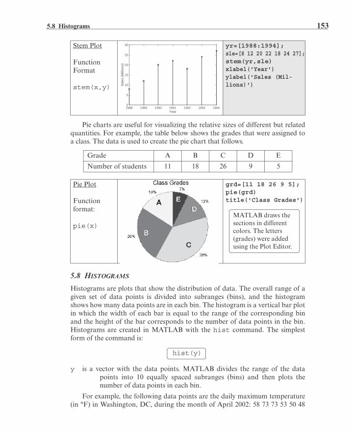
5.8 Histograms 153
Pie charts are useful for visualizing the relative sizes of different but relatedquantities. For example, the table below shows the grades that were assigned toa class. The data is used to create the pie chart that follows.
5.8 HISTOGRAMS
Histograms are plots that show the distribution of data. The overall range of agiven set of data points is divided into subranges (bins), and the histogramshows how many data points are in each bin. The histogram is a vertical bar plotin which the width of each bar is equal to the range of the corresponding binand the height of the bar corresponds to the number of data points in the bin.Histograms are created in MATLAB with the hist command. The simplestform of the command is:
y is a vector with the data points. MATLAB divides the range of the datapoints into 10 equally spaced subranges (bins) and then plots thenumber of data points in each bin.
For example, the following data points are the daily maximum temperature(in °F) in Washington, DC, during the month of April 2002: 58 73 73 53 50 48
Stem Plot
FunctionFormat
stem(x,y)
yr=[1988:1994];sle=[8 12 20 22 18 24 27];stem(yr,sle)xlabel('Year')ylabel('Sales (Mil-lions)')
Grade A B C D E
Number of students 11 18 26 9 5
Pie Plot
Functionformat:
pie(x)
grd=[11 18 26 9 5];pie(grd)title('Class Grades')
Year1988 1989 1990 1991 1992 1993 1994
Sal
es (
Mill
ions
)
0
5
10
15
20
25
30
MATLAB draws the sections in different colors. The letters (grades) were added using the Plot Editor.
hist(y)

154 Chapter 5: Two-Dimensional Plots
56 73 73 66 69 63 74 82 84 91 93 89 91 80 59 69 56 64 63 66 64 74 63 69 (datafrom the U.S. National Oceanic and Atmospheric Administration). A histogramof this data is obtained with the commands:
The plot that is generated is shown in Figure 5-11 (the axis titles were addedusing the Plot Editor). The smallest value in the data set is 48 and the largest is93, which means that the range is 45 and the width of each bin is 4.5. The rangeof the first bin is from 48 to 52.5 and contains two points. The range of the sec-ond bin is from 52.5 to 57 and contains three points, and so on. Two of the bins(75 to 79.5 and 84 to 88.5) do not contain any points.
Since the division of the data range into 10 equally spaced bins might not bethe division that is preferred by the user, the number of bins can be defined to bedifferent than 10. This can be done either by specifying the number of bins, orby specifying the center point of each bin as shown in the following two forms ofthe hist command:
nbins is a scalar that defines the number of bins. MATLAB divides the rangein equally spaced subranges.
x is a vector that specifies the location of the center of each bin (the dis-tance between the centers does not have to be the same for all the bins).The edges of the bins are at the middle point between the centers.
>> y=[58 73 73 53 50 48 56 73 73 66 69 63 74 82 84 91 93 8991 80 59 69 56 64 63 66 64 74 63 69];
>> hist(y)
Figure 5-11: Histogram of temperature data.
Temperature (F)40 50 60 70 80 90 100
Num
ber o
f day
s
0
1
2
3
4
5
6
7
hist(y,nbins) hist(y,x)or

5.8 Histograms 155
In the example above the usermight prefer to divide the temperaturerange into three bins. This can be donewith the command:
As shown in the top graph, the histo-gram that is generated has threeequally spaced bins.
The number and width of the binscan also be specified by a vector xwhose elements define the centers ofthe bins. For example, shown in thelower graph is a histogram that dis-plays the temperature data from abovein six bins with an equal width of 10degrees. The elements of the vector xfor this plot are 45, 55, 65, 75, 85, and95. The plot was obtained with the following commands:
The hist command can be used with options that provide numerical out-put in addition to plotting a histogram. An output of the number of data pointsin each bin can be obtained with one of the following commands:
The output n is a vector. The number of elements in n is equal to the number ofbins, and the value of each element of n is the number of data points (frequencycount) in the corresponding bin. For example, the histogram in Figure 5-11 canalso be created with the following command:
The vector n shows that the first bin has two data points, the second bin hasthree data points, and so on.
>> hist(y,3)
>> x=[45:10:95]
x = 45 55 65 75 85 95
>> hist(y,x)
>> n = hist(y)
n = 2 3 2 7 3 6 0 3 0 4
Temperature (F)40 50 60 70 80 90 100
Num
ber
of d
ays
0
2
4
6
8
10
12
14
Temperature (F)45 55 65 75 85 95
Num
ber
of d
ays
0
2
4
6
8
10
n=hist(y,nbins) n=hist(y,x)n=hist(y)
The vector n shows how many elements are in each bin.

156 Chapter 5: Two-Dimensional Plots
An additional, optional numerical output is the location of the bins. Thisoutput can be obtained with one of the following commands:
xout is a vector in which the value of each element is the location of the centerof the corresponding bin. For example, for the histogram in Figure 5-11:
The vector xout shows that the center of the first bin is at 50.25, the center ofthe second bin is at 54.75, and so on.
5.9 POLAR PLOTS
Polar coordinates, in which the position of a point in aplane is defined by the angle and the radius (distance)to the point, are frequently used in the solution of scienceand engineering problems. The polar command is usedto plot functions in polar coordinates. The command hasthe form:
where theta and radius are vectors whose elements define the coordinates ofthe points to be plotted. The polar command plots the points and draws thepolar grid. The line specifiers are the same as in the plot command. To plot afunction in a certain domain, a vector for values of is created first,and then a vector r with the corresponding values of is created using ele-ment-by-element calculations. The two vectors are then used in the polar com-mand.
>> [n xout]=hist(y)
n = 2 3 2 7 3 6 0 3 0 4
xout = 50.2500 54.7500 59.2500 63.7500 68.2500 72.750077.2500 81.7500 86.2500 90.7500
[n xout]=hist(y,nbins)[n xout]=hist(y)
polar(theta,radius,‘line specifiers’)
(Optional) Specifiers that define the type and color of the line and markers.
Vector Vector
r f=
f
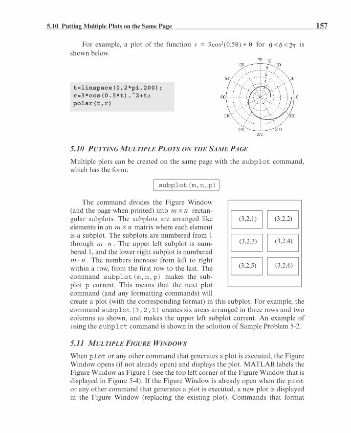
5.10 Putting Multiple Plots on the Same Page 157
For example, a plot of the function for isshown below.
5.10 PUTTING MULTIPLE PLOTS ON THE SAME PAGE
Multiple plots can be created on the same page with the subplot command,which has the form:
The command divides the Figure Window(and the page when printed) into rectan-gular subplots. The subplots are arranged likeelements in an matrix where each elementis a subplot. The subplots are numbered from 1through . The upper left subplot is num-bered 1, and the lower right subplot is numbered
. The numbers increase from left to rightwithin a row, from the first row to the last. Thecommand subplot(m,n,p) makes the sub-plot p current. This means that the next plotcommand (and any formatting commands) willcreate a plot (with the corresponding format) in this subplot. For example, thecommand subplot(3,2,1) creates six areas arranged in three rows and twocolumns as shown, and makes the upper left subplot current. An example ofusing the subplot command is shown in the solution of Sample Problem 5-2.
5.11 MULTIPLE FIGURE WINDOWS
When plot or any other command that generates a plot is executed, the FigureWindow opens (if not already open) and displays the plot. MATLAB labels theFigure Window as Figure 1 (see the top left corner of the Figure Window that isdisplayed in Figure 5-4). If the Figure Window is already open when the plotor any other command that generates a plot is executed, a new plot is displayedin the Figure Window (replacing the existing plot). Commands that format
r 3 0.5cos2 +=
t=linspace(0,2*pi,200);r=3*cos(0.5*t).^2+t;polar(t,r)
subplot(m,n,p)
(3,2,1) (3,2,2)
(3,2,3)
(3,2,5)
(3,2,4)
(3,2,6)
m n
m n
m n
m n
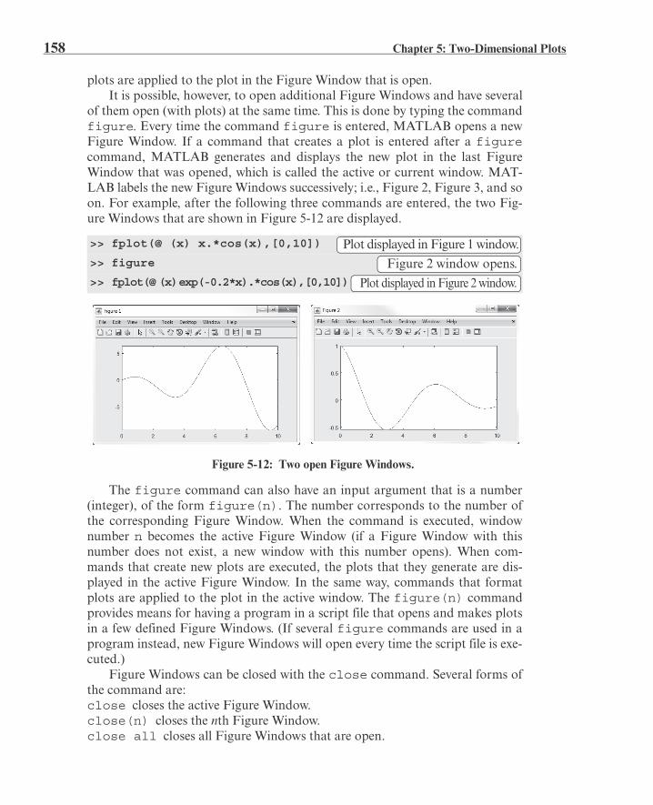
158 Chapter 5: Two-Dimensional Plots
plots are applied to the plot in the Figure Window that is open.It is possible, however, to open additional Figure Windows and have several
of them open (with plots) at the same time. This is done by typing the commandfigure. Every time the command figure is entered, MATLAB opens a newFigure Window. If a command that creates a plot is entered after a figurecommand, MATLAB generates and displays the new plot in the last FigureWindow that was opened, which is called the active or current window. MAT-LAB labels the new Figure Windows successively; i.e., Figure 2, Figure 3, and soon. For example, after the following three commands are entered, the two Fig-ure Windows that are shown in Figure 5-12 are displayed.
The figure command can also have an input argument that is a number(integer), of the form figure(n). The number corresponds to the number ofthe corresponding Figure Window. When the command is executed, windownumber n becomes the active Figure Window (if a Figure Window with thisnumber does not exist, a new window with this number opens). When com-mands that create new plots are executed, the plots that they generate are dis-played in the active Figure Window. In the same way, commands that formatplots are applied to the plot in the active window. The figure(n) commandprovides means for having a program in a script file that opens and makes plotsin a few defined Figure Windows. (If several figure commands are used in aprogram instead, new Figure Windows will open every time the script file is exe-cuted.)
Figure Windows can be closed with the close command. Several forms ofthe command are:close closes the active Figure Window.close(n) closes the nth Figure Window.close all closes all Figure Windows that are open.
>> fplot(@ (x) x.*cos(x),[0,10])
>> figure
>> fplot(@ (x) exp(-0.2*x).*cos(x),[0,10])
Figure 5-12: Two open Figure Windows.
Plot displayed in Figure 1 window.
Figure 2 window opens.
Plot displayed in Figure 2 window.

5.12 Plotting Using the Plots Toolstrip 159
5.12 PLOTTING USING THE PLOTS TOOLSTRIP
Plots can also be constructed interactively by using the PLOTS Toolstrip in theCommand Window. The PLOTS Toolstrip, as shown in Fig. 5-13, is displayedwhen the PLOTS tab is selected. To make a two-dimensional plot, the vectorswith the data points that will be used for the plot have to be already assignedand displayed in the Workspace Window (see Section 4.1). To make a plot,select a variable in the Workspace Window and then, holding the CTRL key,select any additional variables needed. Once a selection of variables has beenmade, the Toolstrip shows icons with images of plot types that can be createdwith the selected variables (e.g. line graph, scatter plot, bar graph, pie chart,etc.). Clicking on an icon opens a Figure Window with the corresponding figuredisplayed. In addition, the MATLAB command that created the plot is dis-played in the Command Window. The user can then copy the command andpaste it into a script file such that in the future the same figure will be createdwhen the script file is executed. On the right side of the Toolstrip the user canchoose to view different plot types in the same Figure Window (Reuse Figure),or to view a new figure type in a new Figure Window (New Figure), such thatfigure types can be compared side by side.
Using the Plots Toolstrip is useful when the user wants to examine differentplot options for given data. For example, Figure 5-13 shows the default layoutof MATLAB with the PLOTS Toolstrip displayed. In the Command Window,the sales data from Section 5.1.1 are assigned to two vectors yr and sle. Thevectors are also displayed (and selected) in the Workspace Window. Icons withimages of various type of plots that can be created are displayed in the PLOTSToolstrip at the top. Additional types of plots can be displayed by clicking onthe down-arrow on the right.
Figure 5-13: Using the PLOTS Toolstrip.

160 Chapter 5: Two-Dimensional Plots
As an example, two different figures, one with line plot and the other withbar plot, were created using the two vectors yr and sle. The two figures aredisplayed in Figure 5-14 and the commands that created the plots are displayedin the Command Window in Figure 5-13.Additional notes:
• When selecting variables for the plot (in theWorkspace Window), the first to beselected will be the independent variable(horizontal axis) and the second will be thedependent variable (vertical axis). After theselection, the variables can be switched byclicking on the Switch icon.
• If only one variable (vector) is selected for a figure, the values of the vector ele-ments will be plotted versus the number of the element.
5.13 EXAMPLES OF MATLAB APPLICATIONS
Sample Problem 5-2: Piston-crank mechanism
The piston-rod-crank mechanism is used in many engineering applications. Inthe mechanism shown in the following figure, the crank is rotating at a constantspeed of 500 rpm.
Calculate and plot the position, velocity, and acceleration of the piston for one
Figure 5-14: Using the PLOTS Toolstrip.

5.13 Examples of MATLAB Applications 161
revolution of the crank. Make the three plots on the same page. Set when t = 0.
Solution
The crank is rotating with a constant angular velocity . This means that if we
set = 0° when t = 0, then at time t the angle is given by , and means
that at all times.The distances d1 and h are given
by:
and
With h known, the distance d2 can becalculated using the PythagoreanTheorem:
The position x of the piston is then given by:
The derivative of x with respect to time gives the velocity of the piston:
The second derivative of x with respect to time gives the acceleration of the pis-ton:
In the equation above, was taken to be zero.A MATLAB program (script file) that calculates and plots the position,
velocity, and acceleration of the piston for one revolution of the crank is shownbelow.
THDrpm=500; r=0.12; c=0.25;
THD=THDrpm*2*pi/60;
tf=2*pi/THD;
t=linspace(0,tf,200);
TH=THD*t;
d2s=c^2-r^2*sin(TH).^2;
x=r*cos(TH)+sqrt(d2s);
xd=-r*THD*sin(TH)-(r^2*THD*sin(2*TH))./(2*sqrt(d2s));
0=
d1 rcos= h r sin=
Define , r, and c.
Change the units of from rpm to rad/s.Calculate the time for one revolution of the crank.
Create a vector for the time with 200 elements.
Calculate for each t.
Calculate d2 squared for each .
Calculate x for each .

162 Chapter 5: Two-Dimensional Plots
When the script file runs it generates the three plots on the same page asshown in Figure 5-13. The figure nicely shows that the velocity of the piston iszero at the end points of the travel range where the piston changes the directionof the motion. The acceleration is maximum (directed to the left) when the pis-ton is at the right end.
xdd=-r*THD^2*cos(TH)-(4*r^2*THD^2*cos(2*TH).*d2s+(r^2*sin(2*TH)*THD).^2)./(4*d2s.^(3/2));
subplot(3,1,1)
plot(t,x)
grid
xlabel('Time (s)')
ylabel('Position (m)')
subplot(3,1,2)
plot(t,xd)
grid
xlabel('Time (s)')
ylabel('Velocity (m/s)')
subplot(3,1,3)
plot(t,xdd)
grid
xlabel('Time (s)')
ylabel('Acceleration (m/s^2)')
Figure 5-15: Position, velocity, and acceleration of the piston vs. time.
Calculate and for each .
Plot x vs. t.
Format the first plot.
Plot vs. t.Format the second plot.
Plot vs. t.
Format the third plot.
Time (s)0 0.02 0.04 0.06 0.08 0.1 0.12
Pos
ition
(m
)
0.1
0.2
0.3
0.4
Time (s)0 0.02 0.04 0.06 0.08 0.1 0.12
Vel
ocity
(m
/s)
-10
0
10
Time (s)0 0.02 0.04 0.06 0.08 0.1 0.12
Acc
eler
atio
n (m
/s2)
-500
0
500

5.13 Examples of MATLAB Applications 163
Sample Problem 5-3: Electric Dipole
The electric field at a point due to a charge is a vector Ewith magnitude E given by Coulomb’s law:
where is the permittivity
constant, q is the magnitude of the charge, and r is thedistance between the charge and the point. The direc-tion of E is along the line that connects the charge withthe point. E points outward from q if q is positive, andtoward q if q is negative. An electric dipole is created when a positive charge anda negative charge of equal magnitude are placed some distance apart. The elec-tric field, E, at any point is obtained by superposition of the electric field of eachcharge.
An electric dipole with
C is created, as shown inthe figure. Determine and plot themagnitude of the electric field alongthe x axis from cm to
cm.
SolutionThe electric field E at any point (x, 0)along the x axis is obtained by addingthe electric field vectors due to each ofthe charges.
E = E–+ E+The magnitude of the electric field isthe length of the vector E.
The problem is solved by following these steps:
Step 1: Create a vector x for points along the x axis.
Step 2: Calculate the distance (and distance squared) from each charge to thepoints on the x axis.
Step 3: Write unit vectors in the direction from each charge to the points onthe x axis.
E1
4 0----------- q
r2----=
+q
x
y
q(2 cm, 2 cm)( 2 cm, 2 cm)

164 Chapter 5: Two-Dimensional Plots
Step 4: Calculate the magnitude of the vector E– and E+ at each point by
using Coulomb’s law.
Step 5: Create the vectors E– and E+ by multiplying the unit vectors by the
magnitudes.
Step 6: Create the vector E by adding the vectors E– and E+.
Step 7: Calculate E, the magnitude (length) of E.
Step 8: Plot E as a function of x.
A program in a script file that solves the problem is:
When this script file is executed in the Command Window, the following figureis created in the Figure Window:
q=12e-9; epsilon0=8.8541878e-12;
x=[-0.05:0.001:0.05]’;
rminusS=(0.02-x).^2+0.02^2;
rminus=sqrt(rminusS);
rplusS=(x+0.02).^2+0.02^2;rplus=sqrt(rplusS);
EminusUV=[((0.02-x)./rminus), (-0.02./rminus)];
EplusUV=[((x+0.02)./rplus), (0.02./rplus)];
EminusMAG=(q/(4*pi*epsilon0))./rminusS;
EplusMAG=(q/(4*pi*epsilon0))./rplusS;
Eminus=[EminusMAG.*EminusUV(:,1), EminusMAG.*EminusUV(:,2)];
Eplus=[EplusMAG.*EplusUV(:,1), EplusMAG.*EplusUV(:,2)];
E=Eminus+Eplus;
EMAG=sqrt(E(:,1).^2+E(:,2).^2);
plot(x,EMAG,'k','linewidth',1)
xlabel('Position along the x-axis (m)','FontSize',12)
ylabel('Magnitude of the electric field (N/C)','FontSize',12)
title('ELECTRIC FIELD DUE TO AN ELECTRIC DIPOLE','FontSize',12)
Create a column vector x.
Step 2. Each variable is a column vector.
Steps 3 & 4. Each vari-able is a two column matrix. Each row is the vector for the cor-responding x.
Step 5.Step 6.
Step 7.
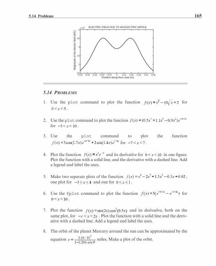
5.14 Problems 165
5.14 PROBLEMS
1. Use the plot command to plot the function for
.
2. Use the plot command to plot the function for .
3. Use the plot command to plot the function
for .
4. Plot the function and its derivative for in one figure.Plot the function with a solid line, and the derivative with a dashed line. Adda legend and label the axes.
5. Make two separate plots of the function ,one plot for and one for .
6. Use the fplot command to plot the function for.
7. Plot the function and its derivative, both on thesame plot, for . Plot the function with a solid line and the deriv-ative with a dashed line. Add a legend and label the axes.
8. The orbit of the planet Mercury around the sun can be approximated by the
equation miles. Make a plot of the orbit.
−0.05 −0.04 −0.03 −0.02 −0.01 0 0.01 0.02 0.03 0.04 0.050.5
1
1.5
2
2.5
3x 10⁵
Position along the x − axis (m)M
agni
tude
of t
he e
lect
ric fi
eld
(N/C
)
ELECTRIC FIELD DUE TO AN ELECTRIC DIPOLE

166 Chapter 5: Two-Dimensional Plots
9. A parametric equation is given by,
Plot the function for . Format the plot such that both axes willrange from –1.5 to 1.5.
10. The butterfly curve (Fay, T. H. "The ButterflyCurve." Amer. Math. Monthly 96, pp. 442-443,1989) is given by the following parametric equa-tions:
On one page make two plots of butterfly curves.One for and the other for .
11. A plot of an astroid is shown in the figure on theright. Make the plot using the Cartesian equation:
12. Make the plot of the astroid that is shown in theprevious problem by using the parametric equa-tion:
and for .
13. Plot the function in the domain . Notice that the
function has a vertical asymptote at . Plot the function by creatingtwo vectors for the domain of x. The first vector (name it x1) includes ele-ments from 0 to 1.9, and the second vector (name it x2) includes elementsfrom 2.1 to 4. For each x vector create a y vector (name them y1 and y2) withthe corresponding values of y according to the function. To plot the func-tion make two curves in the same plot (y1 vs. x1, and y2 vs. x2).
14. Plot the function for . Notice that the function
has two vertical asymptotes. Plot the function by dividing the domain of xinto three parts: one from –4 to near the left asymptote, one between thetwo asymptotes, and one from near the right asymptote to 4. Set the rangeof the y axis from –15 to 15.
x 0.7 10tsin= y 1.2 8tsin=
x-3 -2 -1 0 1 2 3
y
-1
0
1
2
3
-1 -0.5 0 0.5 1-1
-0.5
0
0.5
1
x tcos3= y tsin3=
x 2=

5.14 Problems 167
15. The shape of the heart shown in the figure isgiven by the equation:
Make a plot of the heart.
16. The shape of the pretzel shown is given by thefollowing parametric equations:
where . Make a plot of the pretzel.
17. Make a polar plot of the function:
for The plot, shown in the figure, is Fermat’s spiral.
18. Make a polar plot of the function:
for
The plot is shown on the right.
19. Make a plot (shown) of the function:
(Hint: Rewrite the function in a polar form.)
20. Plot two ellipses is one figure (shown). Theellipse with the solid line has major axes of
and . The ellipse with the dashedline is the solid-line ellipse rotated by 30º.
x-1.5 -1 -0.5 0 0.5 1 1.5
y
-0.5
0
0.5
1
1.5
1
2
3
4
30
210
60
240
90
270
120
300
150
330
180 0
2
4
6
8
10
30
210
60
240
90
270
120
300
150
330
180 0
x-2 -1 0 1 2
y
-2
-1
0
1
2
x-15 -10 -5 0 5 10 15
y
-10
-5
0
5
10
a 10= b 4=

168 Chapter 5: Two-Dimensional Plots
21. The following data gives the height (in inches) of a sunflower plant as afunction of time (days after it was planted).
The height can be modeled by the logistic function:
where H is the height (in.) and t is the time (days). Make a plot of the heightversus time. The figure should show the data from the table above as pointsand the height modeled by the equation as a solid line. Add a legend, andlabel the axes.
22. The voltage t seconds after closing the switchin the circuit shown is given by:
Plot as a function of t for s. Label theaxes. V, , and F.
23. The force F (in N) acting between a particle with acharge q and a round disk with a radius R and acharge Q is given by the equation:
where C2/(N-m2) is the permittiv-ity constant and z is the distance to the particle.
Consider the case where C,
C, and m. Make a plot of F as a function of z form. Use MATLAB’s built-in function max to find the maximum
value of F and the corresponding distance z.
24. The curvilinear motion of a particle isdefined by the following parametric equa-tions:
m mThe velocity of the particle is given by
, where and .
For s make one plot that showsthe position of the particle (y versus x)and a second plot (on the same page) ofthe velocity of the particle as a function of time. In addition, by using MAT-
Time (days) 10 20 30 40 50 60 70Height (in.) 9 22 44 63 80 94 97
VC
VC
V0 36= R 2 500,= C 1 200,=
R
z
R 0.1=
0 50 1000
20
40
60
80
100
120
x (m)
y (m
)

5.14 Problems 169
LAB’s min function, determine the time at which the velocity is the lowest,and the corresponding position of the particle. Using an asterisk marker,show the position of the particle in the first plot. For time use a vector withspacing of 0.1 s.
25. The height and speed of a projectile shoot at aspeed v0 at an angle as a function of time aregiven by:
where m/s2. Determine the time thatthe projectile will hit the ground and plot the height and the speed as a func-tion of time (two plots on one page) for the case that m/s and
. Add titles and label the axes.
26. The position x as a function of time of a particle that moves along a straightline is given by:
ft
The velocity v(t) of the particle is determined by the derivative of x(t) withrespect to t, and the acceleration a(t) is determined by the derivative of v(t)with respect to t.
Derive the expressions for the velocity and acceleration of the particle,and make plots of the position, velocity, and acceleration as functions oftime for s. Use the subplot command to make the three plots onthe same page with the plot of the position on the top, the velocity in themiddle, and the acceleration at the bottom. Label the axes appropriatelywith the correct units.
27. According to Planck’s law of black-body radiation, the spectral energydensity R as a function of wavelength (m) and temperature T (K) is given by:
where m/s is the speed of
light, J-s is the Planck
constant, and J/K isBoltzmann constant. Make the shown figure that contains plots of R as afunction of for m for three temperatures T=3,000 K, T=4,000K, and T=5,000 K.

170 Chapter 5: Two-Dimensional Plots
28. A high-pass filter passes signals with frequenciesthat are higher than a certain cutoff frequency.In this filter the ratio of the magnitudes of thevoltages is given by:
where is the frequency of the input signal. Given and
F, plot as a function of f for Hz. Use logarith-
mic scale for the horizontal (f) axis and linear scale for the vertical axis.
29. A resistor, R = 4 , and an inductor, L = 1.3 H, are connected in a circuit to avoltage source as shown in Figure (a) (an RL circuit). When the voltage
source applies a rectangular voltage pulse with an amplitude of V = 12 Vand a duration of 0.5 s, as shown in Figure (b), the current i(t) in the circuitas a function of time is given by:
for s
for s
Make a plot of the current as a function of time for s.
30. In a typical tension test a dog-boneshaped specimen is pulled in amachine. During the test, the force Fneeded to pull the specimen and thelength L of a gauge section are measured. This data is used for plotting astress-strain diagram of the material. Two definitions, engineering and true,exist for stress and strain. The engineering stress and strain are
defined by and , where L0 and A0 are the initial gauge
length and the initial cross-sectional area of the specimen, respectively. The
true stress and strain are defined by and .
The following are measurements of force and gauge length from a ten-
Vi Vo
C
R
(a) (b)
L0
F F
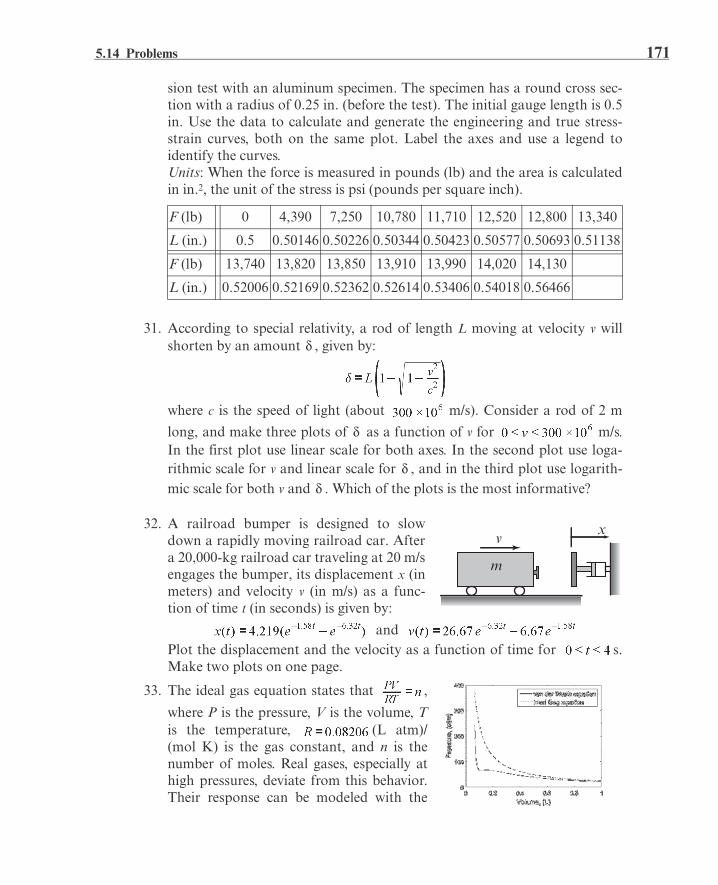
5.14 Problems 171
sion test with an aluminum specimen. The specimen has a round cross sec-tion with a radius of 0.25 in. (before the test). The initial gauge length is 0.5in. Use the data to calculate and generate the engineering and true stress-strain curves, both on the same plot. Label the axes and use a legend toidentify the curves.Units: When the force is measured in pounds (lb) and the area is calculatedin in.2, the unit of the stress is psi (pounds per square inch).
31. According to special relativity, a rod of length L moving at velocity v willshorten by an amount , given by:
where c is the speed of light (about m/s). Consider a rod of 2 m
long, and make three plots of as a function of v for m/s.In the first plot use linear scale for both axes. In the second plot use loga-rithmic scale for v and linear scale for , and in the third plot use logarith-mic scale for both v and . Which of the plots is the most informative?
32. A railroad bumper is designed to slowdown a rapidly moving railroad car. Aftera 20,000-kg railroad car traveling at 20 m/sengages the bumper, its displacement x (inmeters) and velocity v (in m/s) as a func-tion of time t (in seconds) is given by:
and Plot the displacement and the velocity as a function of time for s.Make two plots on one page.
33. The ideal gas equation states that ,
where P is the pressure, V is the volume, Tis the temperature, (L atm)/(mol K) is the gas constant, and n is thenumber of moles. Real gases, especially athigh pressures, deviate from this behavior.Their response can be modeled with the
F (lb) 0 4,390 7,250 10,780 11,710 12,520 12,800 13,340
L (in.) 0.5 0.50146 0.50226 0.50344 0.50423 0.50577 0.50693 0.51138
F (lb) 13,740 13,820 13,850 13,910 13,990 14,020 14,130
L (in.) 0.52006 0.52169 0.52362 0.52614 0.53406 0.54018 0.56466
x
m
v

172 Chapter 5: Two-Dimensional Plots
van der Waals equation , where a and b are material con-
stants. For CO2 L2atm/mol2, and L/mol. Make theshown figure that displays two plots of P versus V for L. Inone plot the pressure is calculated by using the ideal gas equation and theother by using the van der Waals equation. Label the axes and display a leg-end.
34. Two sound waves of slightlydifferent frequencies f1 and f2:
produce sound that is alternat-ing loud and soft. This phe-nomenon, which is calledbeating, is described by theequation:
Make a plot of the beating sound (shown) for s for the case thatHz and Hz.
35. Consider the diode circuit shown in the fig-ure. The current and the voltage canbe determined from the solution of the fol-lowing system of equations:
,
The system can be solved numerically orgraphically. The graphical solution is found by plotting as a function of
from both equations. The solution is the intersection of the two curves.
Make the plots and estimate the solution for the case where A,
V, , and mV.
Time (s)0 0.05 0.1 0.15 0.2 0.25 0.3
Am
plitu
de
-2
-1
0
1
2
R
iDvS
Diode
vD
iD vD
iD
vD
vS 1.5= R 1200=

5.14 Problems 173
36. A monochromatic light that passesthrough a double slit produces on ascreen a diffraction pattern consistingof bright and dark fringes. The inten-sity of the bright fringes, I, as a func-tion of can be calculated by:
where and ,
is the light wave length, a is the width of theslits, and d is the distance between the slits.Plot (as shown) the relative intensity as a function of y (distance to fringes on thescreen) for cm given nm,
mm, and mm. 37. A simply supported beam is
loaded as shown. The shear forceV and bending moment M as afunction of x are given by the fol-lowing equations:
lb
lb-ftfor ft.
lb, lb-ft for ft
lb, lb-ftfor ft.
Plot the shear force and the bending moment as a function of x (two figureson one page such that the shear force diagram is displayed above the bend-ing moment diagram).
38. Biological oxygen demand (BOD) is a measure of the relative oxygen deple-tion effect of a waste contaminant and is widely used to assess the amountof pollution in a water source. The BOD in the effluent ( in mg/L) of arock filter without recirculation is given by:
where is the influent BOD (mg/L), D is the depth of the filter (m), and Q
is the hydraulic flow rate [L/(m2-day)]. Assuming L/(m2-day) plotthe effluent BOD as a function of the depth of the filter ( m)
Distance (cm)-4 -3 -2 -1 0 1 2 3 4
Rel
ativ
e In
tens
ity
0
0.2
0.4
0.6
0.8
1
x
y200 lb/ft
250 lb/ft
20 ft
8 ft12 ft
Lc
L0
Q 300=
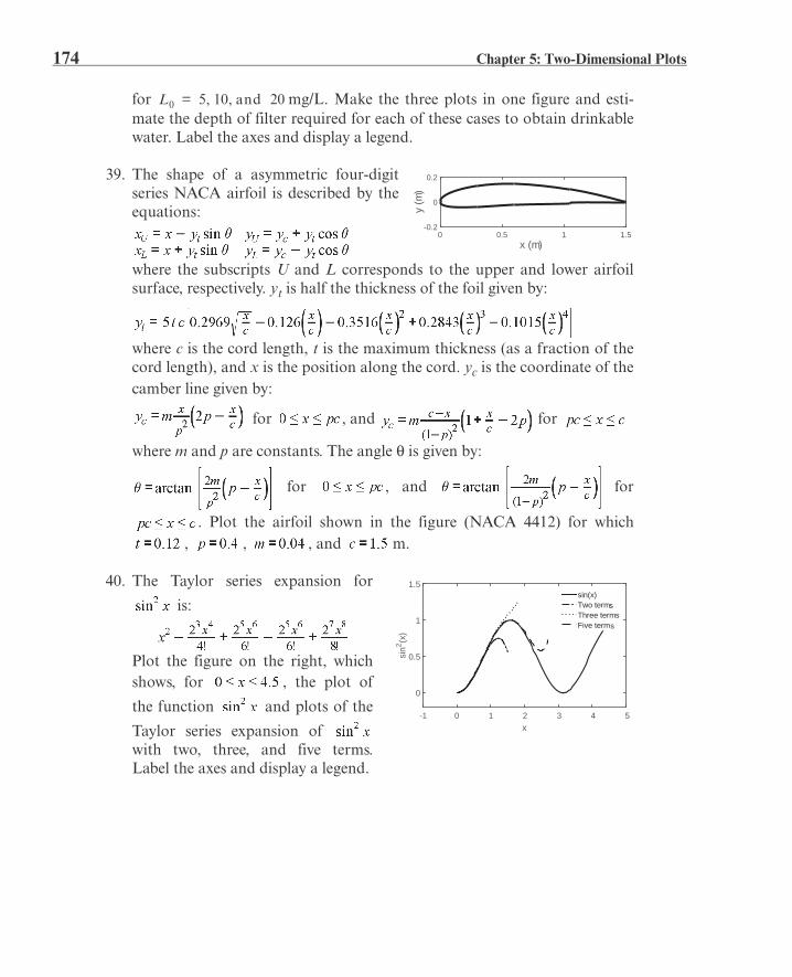
174 Chapter 5: Two-Dimensional Plots
for mg/L. Make the three plots in one figure and esti-mate the depth of filter required for each of these cases to obtain drinkablewater. Label the axes and display a legend.
39. The shape of a asymmetric four-digitseries NACA airfoil is described by theequations:
where the subscripts U and L corresponds to the upper and lower airfoilsurface, respectively. yt is half the thickness of the foil given by:
where c is the cord length, t is the maximum thickness (as a fraction of thecord length), and x is the position along the cord. yc is the coordinate of thecamber line given by:
for , and for
where m and p are constants. The angle is given by:
for , and for
. Plot the airfoil shown in the figure (NACA 4412) for which, , , and m.
40. The Taylor series expansion for
is:
Plot the figure on the right, whichshows, for , the plot of
the function and plots of the
Taylor series expansion of with two, three, and five terms.Label the axes and display a legend.
L0 5 10 and 20, ,=
x (m)0 0.5 1 1.5
y (m
)
-0.2
0
0.2
x-1 0 1 2 3 4 5
sin2 (x
)
0
0.5
1
1.5sin(x)Two termsThree term sFive terms
175
Chapter 6 Programming in MATLAB
A computer program is a sequence of computer commands. In a simple pro-gram the commands are executed one after the other in the order they are typed.In this book, for example, all the programs that have been presented so far inscript files are simple programs. Many situations, however, require more sophis-ticated programs in which commands are not necessarily executed in the orderthey are typed, or different commands (or groups of commands) are executedwhen the program runs with different input variables. For example, a computerprogram that calculates the cost of mailing a package uses different mathemati-cal expressions to calculate the cost depending on the weight and size of thepackage, the content (books are less expensive to mail), and the type of service(airmail, ground, etc.). In other situations there might be a need to repeat asequence of commands several times within a program. For example, programsthat solve equations numerically repeat a sequence of calculations until the errorin the answer is smaller than some measure.
MATLAB provides several tools that can be used to control the flow of aprogram. Conditional statements (Section 6.2) and the switch structure (Sec-tion 6.3) make it possible to skip commands or to execute specific groups ofcommands in different situations. For loops and while loops (Section 6.4)make it possible to repeat a sequence of commands several times.
It is obvious that changing the flow of a program requires some kind ofdecision-making process within the program. The computer must decidewhether to execute the next command or to skip one or more commands andcontinue at a different line in the program. The program makes these decisionsby comparing values of variables. This is done by using relational and logicaloperators, which are explained in Section 6.1. It should also be noted that user-defined functions (introduced in Chapter7) can be used in programming. A user-defined function can be used as a sub-program. When the main program reaches the command line that has the user-defined function, it provides input to the function and “waits” for the results.

176 Chapter 6: Programming in MATLAB
The user-defined function carries out the calculations and transfers the resultsback to the main program, which then continues to the next command.
6.1 RELATIONAL AND LOGICAL OPERATORS
A relational operator compares two numbers by determining whether a compar-ison statement (e.g., 5 < 8) is true or false. If the statement is true, it is assigned avalue of 1. If the statement is false, it is assigned a value of 0. A logical operatorexamines true/false statements and produces a result that is true (1) or false (0)according to the specific operator. For example, the logical AND operator gives1 only if both statements are true. Relational and logical operators can be usedin mathematical expressions and, as will be shown in this chapter, are frequentlyused in combination with other commands to make decisions that control theflow of a computer program.
Relational operators:
Relational operators in MATLAB are:
Note that the “equal to” relational operator consists of two = signs (with nospace between them), since one = sign is the assignment operator. In other rela-tional operators that consist of two characters, there also is no space betweenthe characters (<=, >=, ~=).
• Relational operators are used as arithmetic operators within a mathematicalexpression. The result can be used in other mathematical operations, in address-ing arrays, and together with other MATLAB commands (e.g., if) to controlthe flow of a program.
• When two numbers are compared, the result is 1 (logical true) if the comparison,according to the relational operator, is true, and 0 (logical false) if the compari-son is false.
• If two scalars are compared, the result is a scalar 1 or 0. If two arrays are com-pared (only arrays of the same size can be compared), the comparison is doneelement-by-element, and the result is a logical array of the same size with 1s and0s according to the outcome of the comparison at each address.
• If a scalar is compared with an array, the scalar is compared with every element
Relational operator Description
< Less than
> Greater than
<= Less than or equal to
>= Greater than or equal to
= = Equal to
~= Not Equal to
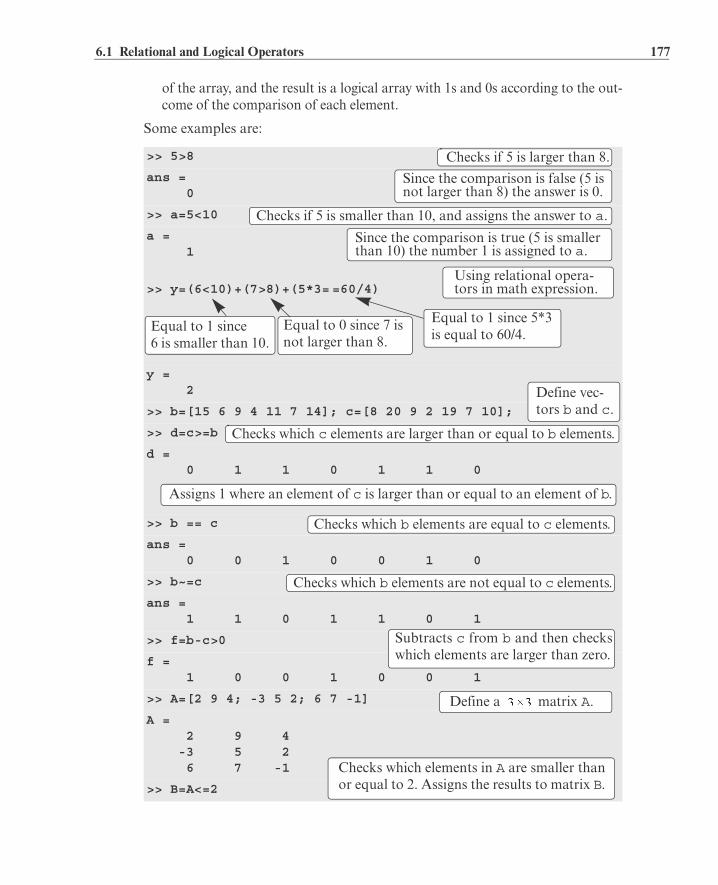
6.1 Relational and Logical Operators 177
of the array, and the result is a logical array with 1s and 0s according to the out-come of the comparison of each element.
Some examples are:
>> 5>8
ans = 0
>> a=5<10
a = 1
>> y=(6<10)+(7>8)+(5*3= =60/4)
y = 2
>> b=[15 6 9 4 11 7 14]; c=[8 20 9 2 19 7 10];
>> d=c>=b
d = 0 1 1 0 1 1 0
>> b == c
ans = 0 0 1 0 0 1 0
>> b~=c
ans = 1 1 0 1 1 0 1
>> f=b-c>0
f = 1 0 0 1 0 0 1
>> A=[2 9 4; -3 5 2; 6 7 -1]
A = 2 9 4 -3 5 2 6 7 -1
>> B=A<=2
Checks if 5 is larger than 8.
Since the comparison is false (5 is not larger than 8) the answer is 0.
Checks if 5 is smaller than 10, and assigns the answer to a.
Since the comparison is true (5 is smaller than 10) the number 1 is assigned to a.
Using relational opera-tors in math expression.
Equal to 1 since6 is smaller than 10.
Equal to 0 since 7 isnot larger than 8.
Equal to 1 since 5*3 is equal to 60/4.
Define vec-tors b and c.
Checks which c elements are larger than or equal to b elements.
Assigns 1 where an element of c is larger than or equal to an element of b.
Checks which b elements are equal to c elements.
Checks which b elements are not equal to c elements.
Subtracts c from b and then checkswhich elements are larger than zero.
Define a matrix A.
Checks which elements in A are smaller thanor equal to 2. Assigns the results to matrix B.

178 Chapter 6: Programming in MATLAB
• The results of a relational operation with vectors, which are vectors with 0s and1s, are called logical vectors and can be used for addressing vectors. When a log-ical vector is used for addressing another vector, it extracts from that vector theelements in the positions where the logical vector has 1s. For example:
• Numerical vectors and arrays with the numbers 0s and 1s are not the same aslogical vectors and arrays with 0s and 1s. Numerical vectors and arrays can notbe used for addressing. Logical vectors and arrays, however, can be used in arith-metic operations. The first time a logical vector or an array is used in arithmeticoperations it is changed to a numerical vector or array.
• Order of precedence: In a mathematical expression that includes relational andarithmetic operations, the arithmetic operations (+, –, *, /, \) have precedenceover relational operations. The relational operators themselves have equal prece-dence and are evaluated from left to right. Parentheses can be used to alter theorder of precedence. Examples are:
B = 1 0 0 1 0 1 0 0 1
>> r = [8 12 9 4 23 19 10]
r = 8 12 9 4 23 19 10
>> s=r<=10
s = 1 0 1 1 0 0 1
>> t=r(s)
t = 8 9 4 10
>> w=r(r<=10)
w = 8 9 4 10
>> 3+4<16/2
ans = 1
>> 3+(4<16)/2
ans = 3.5000
Define a vector r.
Checks which r elements are smaller than or equal to 10.
A logical vector s with 1s at positions where elements of r are smaller than or equal to 10.
Use s for addresses in vector r to create vector t.
Vector t consists of elements ofr in positions where s has 1s.
The same procedure can be done in one step.
+ and / are executed first.
The answer is 1 since 7 < 8 is true.
4 < 16 is executed first, and is equal to 1, since it is true.
3.5 is obtained from 3 + 1/2.
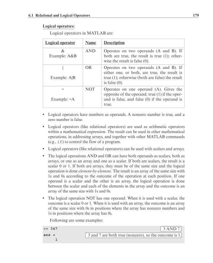
6.1 Relational and Logical Operators 179
Logical operators:
Logical operators in MATLAB are:
• Logical operators have numbers as operands. A nonzero number is true, and azero number is false.
• Logical operators (like relational operators) are used as arithmetic operatorswithin a mathematical expression. The result can be used in other mathematicaloperations, in addressing arrays, and together with other MATLAB commands(e.g., if) to control the flow of a program.
• Logical operators (like relational operators) can be used with scalars and arrays.
• The logical operations AND and OR can have both operands as scalars, both asarrays, or one as an array and one as a scalar. If both are scalars, the result is ascalar 0 or 1. If both are arrays, they must be of the same size and the logicaloperation is done element-by-element. The result is an array of the same size with1s and 0s according to the outcome of the operation at each position. If oneoperand is a scalar and the other is an array, the logical operation is donebetween the scalar and each of the elements in the array and the outcome is anarray of the same size with 1s and 0s.
• The logical operation NOT has one operand. When it is used with a scalar, theoutcome is a scalar 0 or 1. When it is used with an array, the outcome is an arrayof the same size with 0s in positions where the array has nonzero numbers and1s in positions where the array has 0s.
Following are some examples:
Logical operator Name Description
&Example: A&B
AND Operates on two operands (A and B). Ifboth are true, the result is true (1); other-wise the result is false (0).
|
Example: A|B
OR Operates on two operands (A and B). Ifeither one, or both, are true, the result istrue (1); otherwise (both are false) the resultis false (0).
~
Example: ~A
NOT Operates on one operand (A). Gives theopposite of the operand; true (1) if the oper-and is false, and false (0) if the operand istrue.
>> 3&7
ans = 1
3 AND 7.
3 and 7 are both true (nonzero), so the outcome is 1.

180 Chapter 6: Programming in MATLAB
Order of precedence:
Arithmetic, relational, and logical operators can be combined in mathematicalexpressions. When an expression has such a combination, the result depends onthe order in which the operations are carried out. The following is the orderused by MATLAB:
>> a=5|0
a = 1
>> ~25
ans = 0
>> t=25*((12&0)+(~0)+(0|5))
t = 50
>> x=[9 3 0 11 0 15]; y=[2 0 13 -11 0 4];
>> x&yans = 1 0 0 1 0 1
>> z=x|yz = 1 1 1 1 0 1
>> ~(x+y)ans = 0 0 0 1 1 0
Precedence Operation
1 (highest) Parentheses (if nested parentheses exist, inner ones haveprecedence)
2 Exponentiation
3 Logical NOT (~)
4 Multiplication, division
5 Addition, subtraction
6 Relational operators (>, <, >=, <=, = =, ~=)
7 Logical AND (&)
8 (lowest) Logical OR ( | )
5 OR 0 (assign to variable a).
1 is assigned to a since at least one number is true (nonzero).
NOT 25.
The outcome is 0 since 25 is true (nonzero) and the opposite is false.
Using logical operators in a math expression.
Define two vec-tors x and y.
The outcome is a vector with 1 in every position where both x and y are true (nonzero elements), and 0s otherwise.
The outcome is a vector with 1 in every position where either or both x and y are true (nonzero elements), and 0s otherwise.
The outcome is a vector with 0 in every position where the vector x + y is true (nonzero elements), and 1 in every position where x + y is false (zero elements).

6.1 Relational and Logical Operators 181
If two or more operations have the same precedence, the expression is executedin order from left to right.
It should be pointed out here that the order shown above is the one usedsince MATLAB 6. Previous versions of MATLAB used a slightly different order(& did not have precedence over |), so the user must be careful. Compatibilityproblems between different versions of MATLAB can be avoided by usingparentheses even when they are not required.
The following are examples of expressions that include arithmetic, rela-tional, and logical operators:
Built-in logical functions:
MATLAB has built-in functions that are equivalent to the logical operators.These functions are:
and(A,B) equivalent to A&Bor(A,B) equivalent to A|Bnot(A) equivalent to ~A
>> x=-2; y=5;
>> -5<x<-1ans = 0
>> -5<x & x<-1ans = 1
>> ~(y<7)ans = 0
>> ~y<7ans = 1
>> ~((y>=8)|(x<-1))ans = 0
>> ~(y>=8)|(x<-1)ans = 1
Define variables x and y.This inequality is correct mathematically. The answer, however, is false since MATLAB executes from left to right. –5 < x is true (=1) and then 1 < –1 is false (0).
The mathematically correct statement is obtained by using the logical operator &. The inequalities are executed first. Since both are true (1), the answer is 1.
y < 7 is executed first, it is true (1), and ~1 is 0.
~y is executed first, y is true (1) (since y is nonzero), ~1 is 0, and 0 < 7 is true (1).
y >= 8 (false), and x < –1 (true) are exe-cuted first. OR is executed next (true). ~ is executed last, and gives false (0).
y >= 8 (false), and x < –1 (true) are executed first. NOT of (y >= 8) is executed next (true). OR is executed last, and gives true (1).

182 Chapter 6: Programming in MATLAB
In addition, MATLAB has other logical built-in functions, some of which aredescribed in the following table:
Function Description Example
xor(a,b) Exclusive or. Returns true (1) ifone operand is true and theother is false.
>> xor(7,0)ans = 1>> xor(7,-5)ans = 0
all(A) Returns 1 (true) if all elementsin a vector A are true (non-zero). Returns 0 (false) if oneor more elements are false(zero).If A is a matrix, treats columnsof A as vectors, and returns avector with 1s and 0s.
>> A=[6 2 15 9 711];>> all(A)ans = 1>> B=[6 2 15 9 011];>> all(B)ans = 0
any(A) Returns 1 (true) if any elementin a vector A is true (nonzero).Returns 0 (false) if all elementsare false (zero). If A is a matrix, treats columnsof A as vectors, and returns avector with 1s and 0s.
>> A=[6 0 15 0 011];>> any(A)ans = 1>> B = [0 0 0 0 00];>> any(B)ans = 0
find(A)
find(A>d)
If A is a vector, returns the indi-ces of the nonzero elements.
If A is a vector, returns theaddress of the elements thatare larger than d (any rela-tional operator can be used).
>> A=[0 9 4 3 7 0 01 8];>> find(A)ans = 2 3 45 8 9>> find(A>4)ans = 2 5 9
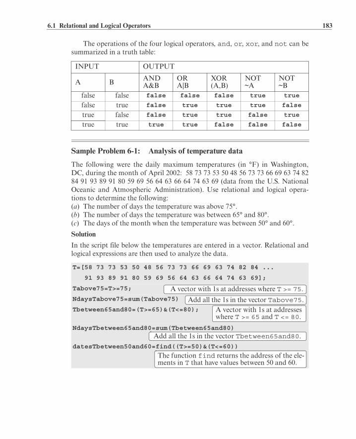
6.1 Relational and Logical Operators 183
The operations of the four logical operators, and, or, xor, and not can besummarized in a truth table:
Sample Problem 6-1: Analysis of temperature data
The following were the daily maximum temperatures (in °F) in Washington,DC, during the month of April 2002: 58 73 73 53 50 48 56 73 73 66 69 63 74 8284 91 93 89 91 80 59 69 56 64 63 66 64 74 63 69 (data from the U.S. NationalOceanic and Atmospheric Administration). Use relational and logical opera-tions to determine the following:(a) The number of days the temperature was above 75°.(b) The number of days the temperature was between 65° and 80°.(c) The days of the month when the temperature was between 50° and 60°.
Solution
In the script file below the temperatures are entered in a vector. Relational andlogical expressions are then used to analyze the data.
INPUT OUTPUT
A B ANDA&B
ORA|B
XOR(A,B)
NOT~A
NOT~B
false false false false false true true
false true false true true true false
true false false true true false true
true true true true false false false
T=[58 73 73 53 50 48 56 73 73 66 69 63 74 82 84 ...
91 93 89 91 80 59 69 56 64 63 66 64 74 63 69];
Tabove75=T>=75;
NdaysTabove75=sum(Tabove75)
Tbetween65and80=(T>=65)&(T<=80);
NdaysTbetween65and80=sum(Tbetween65and80)
datesTbetween50and60=find((T>=50)&(T<=60))
A vector with 1s at addresses where T >= 75.
Add all the 1s in the vector Tabove75.A vector with 1s at addresses where T >= 65 and T <= 80.
Add all the 1s in the vector Tbetween65and80.
The function find returns the address of the ele-ments in T that have values between 50 and 60.
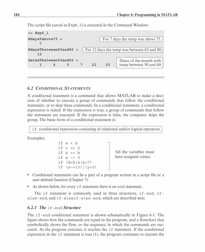
184 Chapter 6: Programming in MATLAB
The script file (saved as Exp6_1) is executed in the Command Window:
6.2 CONDITIONAL STATEMENTS
A conditional statement is a command that allows MATLAB to make a deci-sion of whether to execute a group of commands that follow the conditionalstatement, or to skip these commands. In a conditional statement, a conditionalexpression is stated. If the expression is true, a group of commands that followthe statement are executed. If the expression is false, the computer skips thegroup. The basic form of a conditional statement is:
Examples:if a < bif c >= 5if a == bif a ~= 0if (d<h)&(x>7)if (x~=13)|(y<0)
• Conditional statements can be a part of a program written in a script file or auser-defined function (Chapter 7).
• As shown below, for every if statement there is an end statement.
The if statement is commonly used in three structures, if-end, if-else-end, and if-elseif-else-end, which are described next.
6.2.1 The if-end Structure
The if-end conditional statement is shown schematically in Figure 6-1. Thefigure shows how the commands are typed in the program, and a flowchart thatsymbolically shows the flow, or the sequence, in which the commands are exe-cuted. As the program executes, it reaches the if statement. If the conditionalexpression in the if statement is true (1), the program continues to execute the
>> Exp6_1
NdaysTabove75 = 7
NdaysTbetween65and80 = 12
datesTbetween50and60 = 1 4 5 7 21 23
For 7 days the temp was above 75.
For 12 days the temp was between 65 and 80.
Dates of the month with temp between 50 and 60.
if conditional expression consisting of relational and/or logical operators.
All the variables musthave assigned values.

6.2 Conditional Statements 185
commands that follow the if statement all the way down to the end statement.If the conditional expression is false (0), the program skips the group of com-mands between the if and the end, and continues with the commands that fol-low the end.
The words if and end appear on the screen in blue, and the commandsbetween the if statement and the end statement are automatically indented(they don’t have to be), which makes the program easier to read. An examplewhere the if-end statement is used in a script file is shown in Sample Problem6-2.
Sample Problem 6-2: Calculating worker’s pay
A worker is paid according to his hourly wage up to 40 hours, and 50% more forovertime. Write a program in a script file that calculates the pay to a worker. Theprogram asks the user to enter the number of hours and the hourly wage. Theprogram then displays the pay.
Solution
The program in a script file is shown below. The program first calculates the payby multiplying the number of hours by the hourly wage. Then an if statementchecks whether the number of hours is greater than 40. If so, the next line is exe-cuted and the extra pay for the hours above 40 is added. If not, the programskips to the end.
Figure 6-1: The structure of the if-end conditional statement.
t=input('Please enter the number of hours worked ');
h=input('Please enter the hourly wage in $ ');
Pay=t*h;
if t>40
ifstatement
True
Commands
False
end
......
......
......if conditional expression
........
........
........end..................
A group ofMATLAB commands.
MATLAB program.
MATLAB program.
Flowchart

186 Chapter 6: Programming in MATLAB
Application of the program (in the Command Window) for two cases is shownbelow (the file was saved as Workerpay):
6.2.2 The if-else-end Structure
The if-else-end structure provides a means for choosing one group of com-mands, out of a possible two groups, for execution. The if-else-end struc-ture is shown in Figure 6-2. The figure shows how the commands are typed inthe program, and includes a flowchart that illustrates the flow, or the sequence,
Pay=Pay+(t-40)*0.5*h;
end
fprintf('The worker''s pay is $ %5.2f',Pay)
>> Workerpay
Please enter the number of hours worked 35
Please enter the hourly wage in $ 8
The worker’s pay is $ 280.00
>> Workerpay
Please enter the number of hours worked 50
Please enter the hourly wage in $ 10
The worker’s pay is $ 550.00
Figure 6-2: The structure of the if-else-end conditional statement.
ifstatement
True
Commandsgroup 1
False
end
Commandsgroup 2
......
......
if conditional expression........................
else........................
end............
Group 1 ofMATLAB commands.
MATLAB program.
MATLAB program.
Group 2 ofMATLAB commands.
Flowchart

6.2 Conditional Statements 187
in which the commands are executed. The first line is an if statement with aconditional expression. If the conditional expression is true, the program exe-cutes group 1 of commands between the if and the else statements and thenskips to the end. If the conditional expression is false, the program skips to theelse and then executes group 2 of commands between the else and the end.
6.2.3 The if-elseif-else-end Structure
The if-elseif-else-end structure is shown in Figure 6-3. The figureshows how the commands are typed in the program, and gives a flowchart thatillustrates the flow, or the sequence, in which the commands are executed. Thisstructure includes two conditional statements (if and elseif) that make itpossible to select one out of three groups of commands for execution. The firstline is an if statement with a conditional expression. If the conditional expres-sion is true, the program executes group 1 of commands between the if and the
elseif statements and then skips to the end. If the conditional expression inthe if statement is false, the program skips to the elseif statement. If theconditional expression in the elseif statement is true, the program executesgroup 2 of commands between the elseif and the else and then skips to theend. If the conditional expression in the elseif statement is false, the pro-gram skips to the else and executes group 3 of commands between the elseand the end.
It should be pointed out here that several elseif statements and associ-
Figure 6-3: The structure of the if-elseif-else-end conditional statement.
ifstatement
True
Commandsgroup 1
False
end
Commandsgroup 2
Commandsgroup 3
elseifstatement
True
False
......
......
if conditional expression........................
elseif conditional expression........................
else........................
end............
Group 1 ofMATLAB commands.
MATLAB program.
MATLAB program.
Group 2 ofMATLAB commands.
Flowchart
Group 3 ofMATLAB commands.
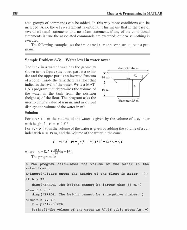
188 Chapter 6: Programming in MATLAB
ated groups of commands can be added. In this way more conditions can beincluded. Also, the else statement is optional. This means that in the case ofseveral elseif statements and no else statement, if any of the conditionalstatements is true the associated commands are executed; otherwise nothing isexecuted.
The following example uses the if-elseif-else-end structure in a pro-gram.
Sample Problem 6-3: Water level in water tower
The tank in a water tower has the geometryshown in the figure (the lower part is a cylin-der and the upper part is an inverted frustumof a cone). Inside the tank there is a float thatindicates the level of the water. Write a MAT-LAB program that determines the volume ofthe water in the tank from the position(height h) of the float. The program asks theuser to enter a value of h in m, and as outputdisplays the volume of the water in m3.
Solution
For m the volume of the water is given by the volume of a cylinderwith height h: .For m the volume of the water is given by adding the volume of a cyl-inder with m, and the volume of the water in the cone:
where .The program is:
% The program calculates the volume of the water in thewater tower.
h=input('Please enter the height of the float in meter ');
if h > 33
disp('ERROR. The height cannot be larger than 33 m.')
elseif h < 0 disp('ERROR. The height cannot be a negative number.')
elseif h <= 19 v = pi*12.5^2*h;
fprintf('The volume of the water is %7.3f cubic meter.\n',v)
V 12.52h=
h 19=

6.3 The switch-case Statement 189
The following is the display in the Command Window when the program is usedwith three different values of water height.
6.3 THE switch-case STATEMENT
The switch-case statement is another method that can be used to direct theflow of a program. It provides a means for choosing one group of commands forexecution out of several possible groups. The structure of the statement is shownin Figure 6-4.The first line is the switch command, which has the form:
The switch expression can be a scalar or a string. Usually it is a variable that hasan assigned scalar or a string. It can also be, however, a mathematical expressionthat includes pre-assigned variables and can be evaluated.• Following the switch command are one or several case commands. Each has
a value (can be a scalar or a string) next to it (value1, value2, etc.) and an associ-ated group of commands below it.
• After the last case command there is an optional otherwise command fol-lowed by a group of commands.
The last line must be an end statement.How does the switch-case statement work?
The value of the switch expression in the switch command is compared withthe values that are next to each of the case statements. If a match is found, thegroup of commands that follow the case statement with the match are exe-cuted. (Only one group of commands—the one between the case that matchesand either the case, otherwise, or end statement that is next—is executed).• If there is more than one match, only the first matching case is executed.
else
rh=12.5+10.5*(h-19)/14; v=pi*12.5^2*19+pi*(h-19)*(12.5^2+12.5*rh+rh^2)/3;
fprintf('The volume of the water is %7.3f cubic meter.\n',v)end
Please enter the height of the float in meter 8The volume of the water is 3926.991 cubic meter.
Please enter the height of the float in meter 25.7The volume of the water is 14114.742 cubic meter.
Please enter the height of the float in meter 35ERROR. The height cannot be larger than 33 m.
switch switch expression
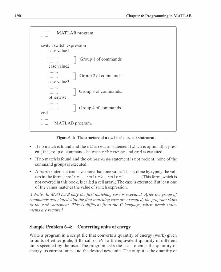
190 Chapter 6: Programming in MATLAB
• If no match is found and the otherwise statement (which is optional) is pres-ent, the group of commands between otherwise and end is executed.
• If no match is found and the otherwise statement is not present, none of thecommand groups is executed.
• A case statement can have more than one value. This is done by typing the val-ues in the form: {value1, value2, value3, ...}. (This form, which isnot covered in this book, is called a cell array.) The case is executed if at least oneof the values matches the value of switch expression.
A Note: In MATLAB only the first matching case is executed. After the group ofcommands associated with the first matching case are executed, the program skipsto the end statement. This is different from the C language, where break state-ments are required.
Sample Problem 6-4: Converting units of energy
Write a program in a script file that converts a quantity of energy (work) givenin units of either joule, ft-lb, cal, or eV to the equivalent quantity in differentunits specified by the user. The program asks the user to enter the quantity ofenergy, its current units, and the desired new units. The output is the quantity of
Figure 6-4: The structure of a switch-case statement.
......
......
switch switch expressioncase value1................case value2................case value3................otherwise................
end............
Group 1 of commands.
MATLAB program.
MATLAB program.
Group 2 of commands.
Group 3 of commands.
Group 4 of commands.

6.3 The switch-case Statement 191
energy in the new units.
The conversion factors are: 1 ft-lb cal eV.Use the program to:(a) Convert 150 J to ft-lb.(b) Convert 2,800 cal to J.(c) Convert 2.7 eV to cal.
Solution
The program includes two sets of switch-case statements and one if-else-end statement. The first switch-case statement is used to convert theinput quantity from its initial units to units of joules. The second is used toconvert the quantity from joules to the specified new units. The if-else-endstatement is used to generate an error message if units are entered incorrectly.
Ein=input('Enter the value of the energy (work) to be converted: ');
EinUnits=input('Enter the current units (J, ft-lb, cal, or eV): ','s');
EoutUnits=input('Enter the new units (J, ft-lb, cal, or eV): ','s');
error=0;
switch EinUnits
case 'J'
EJ=Ein;
case 'ft-lb'
EJ=Ein/0.738;
case 'cal'
EJ=Ein/0.239;
case 'eV'
EJ=Ein/6.24e18;
otherwise
error=1;
end
switch EoutUnits
case 'J'
Eout=EJ;
case 'ft-lb'
Eout=EJ*0.738;
case 'cal'
Eout=EJ*0.239;
case 'eV'
Eout=EJ*6.24e18;
J 0.738= 0.239=
Assign 0 to variable error.First switch statement. Switch expres-sion is a string with initial units.
Each of the four case statementshas a value (string) that correspondsto one of the initial units, and a com-mand that converts Ein to units of J.(Assign the value to EJ.)
Assign 1 to error if no match is found. Possi-ble only if initial units were typed incorrectly.
Second switch statement. Switchexpression is a string with new units.
Each of the four case statementshas a value (string) that correspondsto one of the new units, and a com-mand that converts EJ to the newunits. (Assign the value to Eout.)
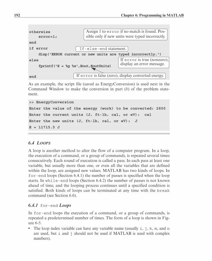
192 Chapter 6: Programming in MATLAB
As an example, the script file (saved as EnergyConversion) is used next in theCommand Window to make the conversion in part (b) of the problem state-ment.
6.4 LOOPS
A loop is another method to alter the flow of a computer program. In a loop,the execution of a command, or a group of commands, is repeated several timesconsecutively. Each round of execution is called a pass. In each pass at least onevariable, but usually more than one, or even all the variables that are definedwithin the loop, are assigned new values. MATLAB has two kinds of loops. Infor-end loops (Section 6.4.1) the number of passes is specified when the loopstarts. In while-end loops (Section 6.4.2) the number of passes is not knownahead of time, and the looping process continues until a specified condition issatisfied. Both kinds of loops can be terminated at any time with the breakcommand (see Section 6.6).
6.4.1 for-end Loops
In for-end loops the execution of a command, or a group of commands, isrepeated a predetermined number of times. The form of a loop is shown in Fig-ure 6-5.• The loop index variable can have any variable name (usually i, j, k, m, and n
are used, but i and j should not be used if MATLAB is used with complexnumbers).
otherwise error=1;
end
if error
disp('ERROR current or new units are typed incorrectly.')
else
fprintf('E = %g %s',Eout,EoutUnits)
end
>> EnergyConversion
Enter the value of the energy (work) to be converted: 2800
Enter the current units (J, ft-lb, cal, or eV): cal
Enter the new units (J, ft-lb, cal, or eV): J
E = 11715.5 J
Assign 1 to error if no match is found. Pos-sible only if new units were typed incorrectly.
If-else-end statement.
If error is true (nonzero), display an error message.
If error is false (zero), display converted energy.

6.4 Loops 193
• In the first pass k = f and the computer executes the commands between thefor and end commands. Then, the program goes back to the for commandfor the second pass. k obtains a new value equal to k = f + s, and the com-mands between the for and end commands are executed with the new value ofk. The process repeats itself until the last pass, where k = t. Then the programdoes not go back to the for, but continues with the commands that follow theend command. For example, if k = 1:2:9, there are five passes, and the corre-sponding values of k are 1, 3, 5, 7, and 9.
• The increment s can be negative (i.e.; k = 25:–5:10 produces four passes withk = 25, 20, 15, 10).
• If the increment value s is omitted, the value is 1 (default) (i.e.; k = 3:7 producesfive passes with k = 3, 4, 5, 6, 7).
• If f = t, the loop is executed once.
• If f > t and s > 0, or if f < t and s < 0, the loop is not executed.
• If the values of k, s, and t are such that k cannot be equal to t, then if s is pos-itive, the last pass is the one where k has the largest value that is smaller than t(i.e., k = 8:10:50 produces five passes with k = 8, 18, 28, 38, 48). If s is negative,the last pass is the one where k has the smallest value that is larger than t.
• In the for command k can also be assigned a specific value (typed as a vector).Example: for k = [7 9 –1 3 3 5].
• The value of k should not be redefined within the loop.
• Each for command in a program must have an end command.
• The value of the loop index variable (k) is not displayed automatically. It is pos-sible to display the value in each pass (which is sometimes useful for debugging)by typing k as one of the commands in the loop.
• When the loop ends, the loop index variable (k) has the value that was lastassigned to it.
Figure 6-5: The structure of a for-end loop.
for k = f:s:t ........ ........ ........end
A group ofMATLAB commands.
Loop index variable.
The value of kin the first pass.
The increment in k after each pass.
The value of k in the last pass.

194 Chapter 6: Programming in MATLAB
A simple example of a for-end loop (in a script file) is:
When this program is executed, the loop is executed four times. The value of k inthe four passes is k = 1, 4, 7, and 10, which means that the values that areassigned to x in the passes are x = 1, 16, 49, and 100, respectively. Since a semi-colon is not typed at the end of the second line, the value of x is displayed in theCommand Window at each pass. When the script file is executed, the display inthe Command Window is:
Sample Problem 6-5: Sum of a series
(a) Use a for-end loop in a script file to calculate the sum of the first n terms
of the series: . Execute the script file for n = 4 and n = 20.
(b) The function sin(x) can be written as a Taylor series by:
Write a user-defined function file that calculates sin(x) by using the Taylor series.For the function name and arguments use y = Tsin(x,n). The input argu-ments are the angle x in degrees and n the number of terms in the series. Use thefunction to calculate sin( ) using three and seven terms.
Solution
(a) A script file that calculates the sum of the first n terms of the series is shownin the following.
for k=1:3:10
x = k^2
end
>> x = 1
x = 16
x = 49
x = 100
k 1=
n
xsink 0=
=

6.4 Loops 195
The summation is done with a loop. In each pass one term of the series is calcu-lated (in the first pass the first term, in the second pass the second term, and soon) and is added to the sum of the previous elements. The file is saved asExp6_5a and then executed twice in the Command Window:
(b) A user-defined function file that calculates sin(x) by adding n terms of a Tay-lor series is shown below.
The first element corresponds to k = 0, which means that in order to add n termsof the series, in the last loop k = n – 1. The function is used in the CommandWindow to calculate sin( ) using three and seven terms:
n=input('Enter the number of terms ' );
S=0;
for k=1:n
S=S+(-1)^k*k/2^k;
end
fprintf('The sum of the series is: %f',S)
>> Exp6_5a
Enter the number of terms 4
The sum of the series is: -0.125000
>> Exp7_5a
Enter the number of terms 20
The sum of the series is: -0.222216
function y = Tsin(x,n)
% Tsin calculates the sin using Taylor formula.
% Input arguments:
% x The angle in degrees, n number of terms.
xr=x*pi/180;
y=0;
for k=0:n-1
y=y+(-1)^k*xr^(2*k+1)/factorial(2*k+1);
end
>> Tsin(150,3)
ans = 0.6523
Setting the sum to zero.In each pass one element of the series is calculated and is added to the sum of the elements from the previous passes.
for-end loop.
Converting the angle from degrees to radians.
for-end loop.
Calculating sin(150 ) with three terms of Taylor series.
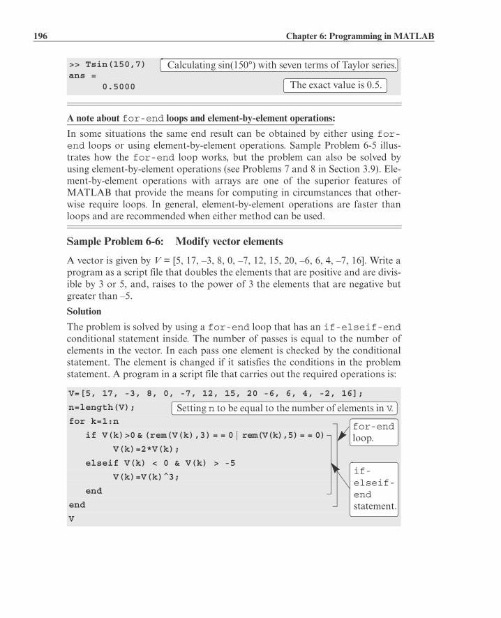
196 Chapter 6: Programming in MATLAB
A note about for-end loops and element-by-element operations:
In some situations the same end result can be obtained by either using for-end loops or using element-by-element operations. Sample Problem 6-5 illus-trates how the for-end loop works, but the problem can also be solved byusing element-by-element operations (see Problems 7 and 8 in Section 3.9). Ele-ment-by-element operations with arrays are one of the superior features ofMATLAB that provide the means for computing in circumstances that other-wise require loops. In general, element-by-element operations are faster thanloops and are recommended when either method can be used.
Sample Problem 6-6: Modify vector elements
A vector is given by V = [5, 17, –3, 8, 0, –7, 12, 15, 20, –6, 6, 4, –7, 16]. Write aprogram as a script file that doubles the elements that are positive and are divis-ible by 3 or 5, and, raises to the power of 3 the elements that are negative butgreater than –5.
Solution
The problem is solved by using a for-end loop that has an if-elseif-endconditional statement inside. The number of passes is equal to the number ofelements in the vector. In each pass one element is checked by the conditionalstatement. The element is changed if it satisfies the conditions in the problemstatement. A program in a script file that carries out the required operations is:
>> Tsin(150,7)ans = 0.5000
V=[5, 17, -3, 8, 0, -7, 12, 15, 20 -6, 6, 4, -2, 16];
n=length(V);
for k=1:n
if V(k)>0 & (rem(V(k),3) = = 0 | rem(V(k),5) = = 0)
V(k)=2*V(k);
elseif V(k) < 0 & V(k) > -5
V(k)=V(k)^3;
end
end
V
Calculating sin(150°) with seven terms of Taylor series.
The exact value is 0.5.
Setting n to be equal to the number of elements in V.
if-elseif-endstatement.
for-end loop.

6.4 Loops 197
The file is saved as Exp6_6 and then executed in the Command Window:
6.4.2 while-end Loops
while-end loops are used in situations when looping is needed but the num-ber of passes is not known in advance. In while-end loops the number ofpasses is not specified when the looping process starts. Instead, the looping pro-cess continues as long as a stated condition is satisfied. The structure of awhile-end loop is shown in Figure 6-6.
The first line is a while statement that includes a conditional expression.When the program reaches this line the conditional expression is checked. If it isfalse (0), MATLAB skips to the end statement and continues with the program.If the conditional expression is true (1), MATLAB executes the group of com-mands that follow between the while and end commands. Then MATLABjumps back to the while command and checks the conditional expression.This looping process continues until the conditional expression is false.
For a while-end loop to execute properly:
• The conditional expression in the while command must include at least onevariable.
• The variables in the conditional expression must have assigned values whenMATLAB executes the while command for the first time.
• At least one of the variables in the conditional expression must be assigned anew value in the commands that are between the while and the end. Other-wise, once the looping starts it will never stop, since the conditional expressionwill remain true.
An example of a simple while-end loop is shown in the following program. Inthis program a variable x with an initial value of 1 is doubled in each pass as
>> Exp6_6
V = 10 17 -27 8 0 -7 24 30 40 -6 12 4-8 16
Figure 6-6: The structure of a while-end loop.
while conditional expression ........ ........ ........end
A group ofMATLAB commands.
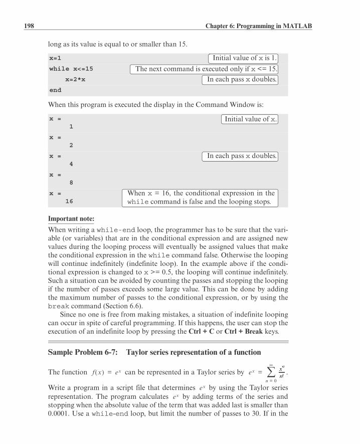
198 Chapter 6: Programming in MATLAB
long as its value is equal to or smaller than 15.
When this program is executed the display in the Command Window is:
Important note:
When writing a while-end loop, the programmer has to be sure that the vari-able (or variables) that are in the conditional expression and are assigned newvalues during the looping process will eventually be assigned values that makethe conditional expression in the while command false. Otherwise the loopingwill continue indefinitely (indefinite loop). In the example above if the condi-tional expression is changed to x >= 0.5, the looping will continue indefinitely.Such a situation can be avoided by counting the passes and stopping the loopingif the number of passes exceeds some large value. This can be done by addingthe maximum number of passes to the conditional expression, or by using thebreak command (Section 6.6).
Since no one is free from making mistakes, a situation of indefinite loopingcan occur in spite of careful programming. If this happens, the user can stop theexecution of an indefinite loop by pressing the Ctrl + C or Ctrl + Break keys.
Sample Problem 6-7: Taylor series representation of a function
The function can be represented in a Taylor series by .
Write a program in a script file that determines by using the Taylor seriesrepresentation. The program calculates by adding terms of the series andstopping when the absolute value of the term that was added last is smaller than0.0001. Use a while-end loop, but limit the number of passes to 30. If in the
x=1
while x<=15
x=2*x
end
x = 1
x = 2
x = 4
x = 8
x = 16
Initial value of x is 1.
The next command is executed only if x <= 15.
In each pass x doubles.
Initial value of x.
In each pass x doubles.
When x = 16, the conditional expression in thewhile command is false and the looping stops.
f x ex= ex
n 0=
=
ex
ex

6.4 Loops 199
30th pass the value of the term that is added is not smaller than 0.0001, the pro-gram stops and displays a message that more than 30 terms are needed.
Use the program to calculate , , and .
Solution
The first few terms of the Taylor series are:
A program that uses the series to calculate the function is shown next. Theprogram asks the user to enter the value of x. Then the first term, an, isassigned the number 1, and an is assigned to the sum S. Then, from the secondterm on, the program uses a while loop to calculate the nth term of the seriesand add it to the sum. The program also counts the number of terms n. Theconditional expression in the while command is true as long as the absolutevalue of the nth an term is larger than 0.0001, and the number of passes n issmaller than 30. This means that if the 30th term is not smaller than 0.0001, thelooping stops.
The program uses an if-else-end statement to display the results. If thelooping stopped because the 30th term is not smaller than 0.0001, it displays amessage indicating this. If the value of the function is calculated successfully, itdisplays the value of the function and the number of terms used. When the pro-gram executes, the number of passes depends on the value of x. The program
(saved as expox) is used to calculate , , and :
x=input('Enter x ' );
n=1; an=1; S=an;
while abs(an) >= 0.0001 & n <= 30
an=x^n/factorial(n);
S=S+an;
n=n+1;
end
if n >= 30
disp('More than 30 terms are needed')
else
fprintf('exp(%f) = %f',x,S)
fprintf('\nThe number of terms used is: %i',n)
end
>> expox
Enter x 2
Start of the while loop.
Calculating the nth term.
Adding the nth term to the sum.
Counting the number of passes.
End of the while loop.
if-else-end loop.
Calculating exp(2).

200 Chapter 6: Programming in MATLAB
6.5 NESTED LOOPS AND NESTED CONDITIONAL STATEMENTS
Loops and conditional statements can be nested within other loops or condi-tional statements. This means that a loop and/or a conditional statement canstart (and end) within another loop or conditional statement. There is no limitto the number of loops and conditional statements that can be nested. It mustbe remembered, however, that each if, case, for, and while statement musthave a corresponding end statement. Figure 6-7 shows the structure of a nested
for-end loop within another for-end loop. In the loops shown in this figure,if, for example, n = 3 and m = 4, then first k = 1 and the nested loop executesfour times with h = 1, 2, 3, 4. Next k = 2 and the nested loop executes again fourtimes with h = 1, 2, 3, 4. Finally k = 3 and the nested loop executes again fourtimes. Every time a nested loop is typed, MATLAB automatically indents thenew loop relative to the outside loop. Nested loops and conditional statementsare demonstrated in the following sample problem.
exp(2.000000) = 7.389046
The number of terms used is: 12
>> expox
Enter x -4
exp(-4.000000) = 0.018307
The number of terms used is: 18
>> expox
Enter x 21
More than 30 terms are needed
Figure 6-7: Structure of nested loops.
12 terms used.
Calculating exp(–4).
18 terms used.
Trying to calculate exp(21).
for k = 1:nfor h = 1:m
........ ........ ........
endend
A group ofcommands.
Nestedloop
Loop
Every time k increases by 1, the nested loop exe-cutes m times. Over-all, the group of commands are exe-cuted n m times.

6.5 Nested Loops and Nested Conditional Statements 201
Sample Problem 6-8: Creating a matrix with a loop
Write a program in a script file that creates an n m matrix with elements thathave the following values. The value of each element in the first row is the num-ber of the column. The value of each element in the first column is the numberof the row. The rest of the elements each has a value equal to the sum of the ele-ment above it and the element to the left. When executed, the program asks theuser to enter values for n and m.
Solution
The program, shown below, has two loops (one nested) and a nested if-elseif-else-end structure. The elements in the matrix are assigned valuesrow by row. The loop index variable of the first loop, k, is the address of the row,and the loop index variable of the second loop, h, is the address of the column.
The program is executed in the Command Window to create a matrix.
n=input('Enter the number of rows ');
m=input('Enter the number of columns ');
A=[];
for k=1:n
for h=1:m
if k==1
A(k,h)=h;
elseif h==1
A(k,h)=k;
else
A(k,h)=A(k,h-1)+A(k-1,h);
end
end
end
A
>> Chap6_exp8
Enter the number of rows 4
Enter the number of columns 5
Define an empty matrix A.
Start of the first for-end loop.
Start of the second for-end loop.
Start of the conditional statement.
Assign values to the elements of the first row.
Assign values to the elements of the first column.
Assign values to other elements.
end of the if statement.
end of the nested for-end loop.
end of the first for-end loop.

202 Chapter 6: Programming in MATLAB
6.6 THE break AND continue COMMANDS
The break command:
• When inside a loop (for or while), the break command terminates the exe-cution of the loop (the whole loop, not just the last pass). When the breakcommand appears in a loop, MATLAB jumps to the end command of the loopand continues with the next command (it does not go back to the for commandof that loop).
• If the break command is inside a nested loop, only the nested loop is termi-nated.
• When a break command appears outside a loop in a script or function file, itterminates the execution of the file.
• The break command is usually used within a conditional statement. In loops itprovides a method to terminate the looping process if some condition is met —for example, if the number of loops exceeds a predetermined value, or an error insome numerical procedure is smaller than a predetermined value. When typedoutside a loop, the break command provides a means to terminate the execu-tion of a file, such as when data transferred into a function file is not consistentwith what is expected.
The continue command:
• The continue command can be used inside a loop (for or while) to stopthe present pass and start the next pass in the looping process.
• The continue command is usually a part of a conditional statement. WhenMATLAB reaches the continue command, it does not execute the remainingcommands in the loop, but skips to the end command of the loop and thenstarts a new pass.
A = 1 2 3 4 5 2 4 7 11 16 3 7 14 25 41 4 11 25 50 91

6.7 Examples of MATLAB Applications 203
6.7 EXAMPLES OF MATLAB APPLICATIONS
Sample Problem 6-9: Withdrawing from a retirement account.
A person in retirement is depositing $300,000 in a saving account that pays 5%interest per year. The person plans to withdraw money from the account once ayear. He starts by withdrawing $25,000 after the first year, and in future years heincreases the amount he withdraws according to the inflation rate. For example,if the inflation rate is 3%, he withdraws $25,750 after the second year. Calculatethe number of years the money in the account will last assuming a constantyearly inflation rate of 2%. Make a plot that shows the yearly withdrawals andthe balance of the account over the years.
Solution
The problem is solved by using a loop (a while loop since the number of passesis not known before the loop starts). In each pass the amount to be withdrawnand the account balance are calculated. The looping continues as long as theaccount balance is larger than or equal to the amount to be withdrawn. The fol-lowing is a program in a script file that solves the problem. In the program,year is a vector in which each element is a year number, W is a vector with theamount withdrawn each year, and AB is a vector with the account balance eachyear.
rate=0.05; inf=0.02;
clear W AB year
year(1)=0;
W(1)=0;
AB(1)=300000;
Wnext=25000;
ABnext=300000*(1 + rate);
n=2;
while ABnext >= Wnext
year(n)=n-1;
W(n)=Wnext;
AB(n)=ABnext-W(n);
ABnext=AB(n)*(1+rate);
Wnext=W(n)*(1+inf);
n=n+1;
end
fprintf('The money will last for %f years',year(n-1))
bar(year,[AB' W'],2.0)
First element is year 0.
Initial withdrawal amount.
Initial account balance.
The amount to be withdrawn after a year.
The account balance after a year.
while checks if the next balance islarger than the next withdrawal.
Amount withdrawn in year n – 1.
Account balance in year n – 1 after withdrawal.The account balance after additional year.
The amount to be withdrawn after an additional year.

204 Chapter 6: Programming in MATLAB
The program is executed in the following Command Window:
The program also generates the following figure (axis labels and legend wereadded to the plot by using the Plot Editor).
Sample Problem 6-10: Creating a random list
Six singers—John, Mary, Tracy, Mike, Katie, and David—are performing in acompetition. Write a MATLAB program that generates a list of a random orderin which the singers will perform.
Solution
An integer (1 through 6) is assigned to each name (1 to John, 2 to Mary, 3 toTracy, 4 to Mike, 5 to Katie, and 6 to David). The program, shown below, firstcreates a list of the integers 1 through 6 in a random order. The integers aremade the elements of six-element vector. This is done by using MATLAB’sbuilt-in function randi (see Section 3.7) for assigning integers to the elementsof the vector. To make sure that all the integers of the elements are differentfrom each other, the integers are assigned one by one. Each integer that is sug-gested by the randi function is compared with all the integers that have beenassigned to previous elements. If a match is found, the integer is not assigned,and randi is used for suggesting a new integer. Since each singer name is asso-ciated with an integer, once the integer list is complete the switch-case state-ment is used to create the corresponding name list.
>> Chap6_exp9
The money will last for 15 years.
clear, clc
n=6;

6.7 Examples of MATLAB Applications 205
The while loop checks that every new integer (element) that is to be added tothe vector L is not equal any of the integers in elements already in the vector L.If a match is found, it keeps generating new integers until the new integer is dif-ferent from all the integers that are already in x.
When the program is executed, the following is displayed in the CommandWindow. Obviously, a list in a different order will be displayed every time theprogram is executed.
L(1)=randi(n);
for p=2:n
L(p)=randi(n);
r=0;
while r==0
r=1;
for k=1:p-1
if L(k)==L(p)
L(p)=randi(n);
r=0;
break
end
end
end
end
for i=1:n switch L(i) case 1 disp('John') case 2 disp('Mary') case 3 disp('Tracy') case 4 disp('Mike') case 5 disp('Katie') case 6 disp('David') endend
The performing order is:
Assign the first integer to L(1).
Assign the next integer to L(p).
Set r to zero.
See explanation below.
Set r to 1.
for loop compares the integer assigned to L(p)to the integers that have been assigned to previous elements.
If a match if found, a new integer is assigned to L(p) and r is set to zero.
The nested for loop is stopped. The pro-gram goes back to the while loop. Since r = 0, the nested loop inside the while loop starts again and checks if the new integer that is assigned to L(p) is equal to an inte-ger that is already in the vector L.
The switch-case state-ment lists the names according to the values of the integers in the ele-ments of L.

206 Chapter 6: Programming in MATLAB
Sample Problem 6-11: Flight of a model rocket
The flight of a model rocket can be modeled as follows.During the first 0.15s the rocket is propelled upward by therocket engine with a force of 16 N. The rocket then flies upwhile slowing down under the force of gravity. After itreaches the apex, the rocket starts to fall back down. Whenits downward velocity reaches 20 m/s, a parachute opens(assumed to open instantly), and the rocket continues todrop at a constant speed of 20 m/s until it hits the ground.Write a program that calculates and plots the speed andaltitude of the rocket as a function of time during the flight.
Solution
The rocket is assumed to be a particle that moves along astraight line in the vertical plane. For motion with constantacceleration along a straight line, the velocity and position as a function of timeare given by:
and
where and are the initial velocity and position, respectively. In the com-puter program the flight of the rocket is divided into three segments. Each seg-ment is calculated in a while loop. In every pass the time increases by anincrement.
Segment 1: The first 0.15s when the rocket engine is on.During this period, the rocket moves up with a constantacceleration. The acceleration is determined by drawinga free body and a mass acceleration diagram (shown onthe right). From Newton’s second law, the sum of theforces in the vertical direction is equal to the mass timesthe acceleration (equilibrium equation):
+Solving the equation for the acceleration gives:
Katie
Tracy
David
Mary
John
Mike
v t v0 at+=
v0 s0
F =

6.7 Examples of MATLAB Applications 207
The velocity and height as a function of time are:
and
where the initial velocity and initial position are both zero. In the computer pro-gram this segment starts at t = 0, and the looping continues as long as s.The time, velocity, and height at the end of this segment are , , and .
Segment 2: The motion from when the engine stops until the parachute opens.In this segment the rocket moves with a constant deceleration g. The speed andheight of the rocket as functions of time are given by:
and
In this segment the looping continues until the velocity of the rocket is –20 m/s(negative since the rocket moves down). The time and height at the end of thissegment are and .
Segment 3: The motion from when the parachute opens until the rocket hits theground. In this segment the rocket moves with constant velocity (zero accelera-tion). The height as a function of time is given by , where
is the constant velocity after the parachute opens. In this segment thelooping continues as long as the height is greater than zero.
A program in a script file that carries out the calculations is shown below.
m=0.05; g=9.81; tEngine=0.15; Force=16; vChute=-20;Dt=0.01;
clear t v h
n=1;
t(n)=0; v(n)=0; h(n)=0;
% Segment 1
a1=(Force-m*g)/m;
while t(n) < tEngine & n < 50000
n=n+1;
t(n)=t(n-1)+Dt;
v(n)=a1*t(n);
h(n)=0.5*a1*t(n)^2;
end
v1=v(n); h1=h(n); t1=t(n);
% Segment 2
while v(n) >= vChute & n < 50000
n=n+1;
t(n)=t(n-1)+Dt;
v t 0 at+=
t1 v1 h1
t2 h2
vchute
The first while loop.
The second while loop.
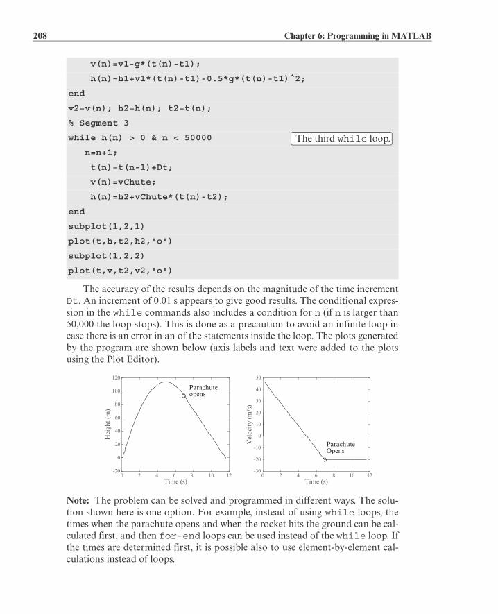
208 Chapter 6: Programming in MATLAB
The accuracy of the results depends on the magnitude of the time incrementDt. An increment of 0.01 s appears to give good results. The conditional expres-sion in the while commands also includes a condition for n (if n is larger than50,000 the loop stops). This is done as a precaution to avoid an infinite loop incase there is an error in an of the statements inside the loop. The plots generatedby the program are shown below (axis labels and text were added to the plotsusing the Plot Editor).
Note: The problem can be solved and programmed in different ways. The solu-tion shown here is one option. For example, instead of using while loops, thetimes when the parachute opens and when the rocket hits the ground can be cal-culated first, and then for-end loops can be used instead of the while loop. Ifthe times are determined first, it is possible also to use element-by-element cal-culations instead of loops.
v(n)=v1-g*(t(n)-t1);
h(n)=h1+v1*(t(n)-t1)-0.5*g*(t(n)-t1)^2;
end
v2=v(n); h2=h(n); t2=t(n);
% Segment 3
while h(n) > 0 & n < 50000
n=n+1;
t(n)=t(n-1)+Dt;
v(n)=vChute;
h(n)=h2+vChute*(t(n)-t2);
end
subplot(1,2,1)
plot(t,h,t2,h2,'o')
subplot(1,2,2)
plot(t,v,t2,v2,'o')
The third while loop.
Time (s)0 2 4 6 8 10 12
Hei
ght
(m)
-20
0
20
40
60
80
100
120
Time (s)0 2 4 6 8 10 12
Vel
ocit
y (m
/s)
-30
-20
-10
0
10
20
30
40
50
Parachuteopens
ParachuteOpens
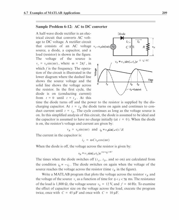
6.7 Examples of MATLAB Applications 209
Sample Problem 6-12: AC to DC converter
A half-wave diode rectifier is an elec-trical circuit that converts AC volt-age to DC voltage. A rectifier circuitthat consists of an AC voltagesource, a diode, a capacitor, and aload (resistor) is shown in the figure.The voltage of the source is
, where , in
which f is the frequency. The opera-tion of the circuit is illustrated in thelower diagram where the dashed lineshows the source voltage and thesolid line shows the voltage acrossthe resistor. In the first cycle, thediode is on (conducting current)from until . At thistime the diode turns off and the power to the resistor is supplied by the dis-charging capacitor. At the diode turns on again and continues to con-duct current until . The cycle continues as long as the voltage source ison. In this simplified analysis of this circuit, the diode is assumed to be ideal andthe capacitor is assumed to have no charge initially (at ). When the diodeis on, the resistor’s voltage and current are given by:
and
The current in the capacitor is:
When the diode is off, the voltage across the resistor is given by:
The times when the diode switches off ( , , and so on) are calculated from
the condition . The diode switches on again when the voltage of thesource reaches the voltage across the resistor (time in the figure).
Write a MATLAB program that plots the voltage across the resistor andthe voltage of the source as a function of time for ms. The resistanceof the load is 1,800 , the voltage source V, and Hz. To examinethe effect of capacitor size on the voltage across the load, execute the programtwice, once with F and once with F.
vs v0 tsin= 2 f=
t 0= t tA=
t tB=t tD=
t 0=
vR v0 tsin=
iC Cv0 tcos=
tA tD
tB
vR
vs
v0 12= f 60=
C 45= C 10=

210 Chapter 6: Programming in MATLAB
Solution
A program that solves the problem is presented below. The program has twoparts—one that calculates the voltage when the diode is on, and the otherwhen the diode is off. The switch command is used for switching between thetwo parts. The calculations start with the diode on (the variable state=‘on’),and when the value of state is changed to ‘off’, and the programswitches to the commands that calculate for this state. These calculationscontinue until , when the program switches back to the equations that arevalid when the diode is on.
V0=12; C=45e-6; R=1800; f=60;
Tf=70e-3; w=2*pi*f;
clear t VR Vs
t=0:0.05e-3:Tf;
n=length(t);
state='on'
for i=1:n
Vs(i)=V0*sin(w*t(i));
switch state
case 'on'
VR(i)=Vs(i);
iR=Vs(i)/R;
iC=w*C*V0*cos(w*t(i));
sumI=iR+iC;
if sumI <= 0
state='off ';
tA=t(i);
end
case 'off '
VR(i)=V0*sin(w*tA)*exp(-(t(i)-tA)/(R*C));
if Vs(i) >= VR(i)
state='on';
end
end
end
plot(t,Vs,':',t,VR,'k','linewidth',1)
xlabel('Time (s)'); ylabel('Voltage (V)')
vR
vR
Assign ‘on’ to the variable state.
Calculate the voltage of the source at time t.
Diode is on.
Check if .
If true, assign ‘off’ to state.
Assign a value to .tA
Diode is off.
Check if .
If true, assign ‘on’ to the variable state.
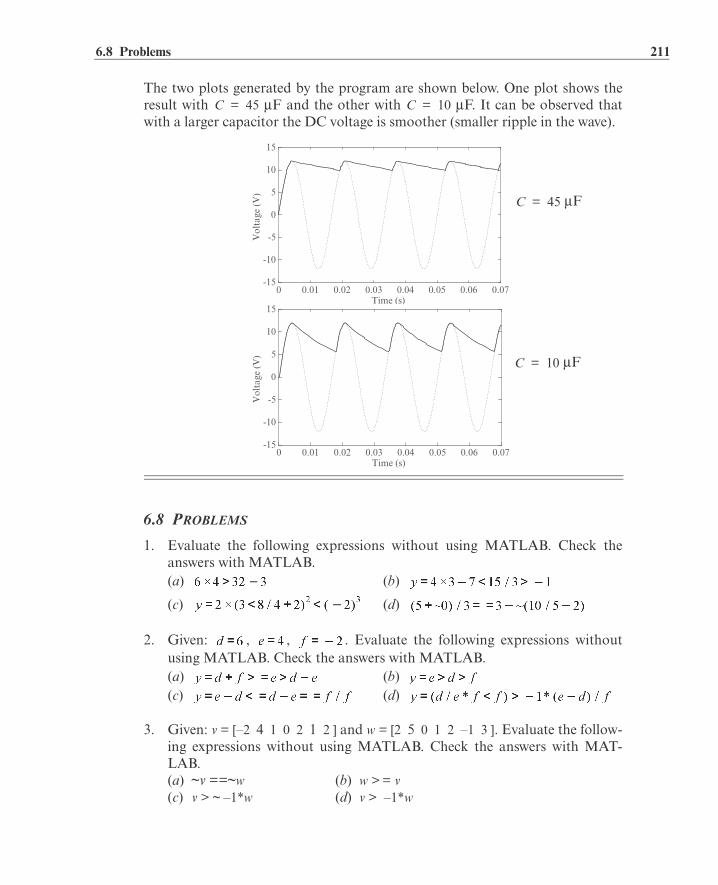
6.8 Problems 211
The two plots generated by the program are shown below. One plot shows theresult with F and the other with F. It can be observed thatwith a larger capacitor the DC voltage is smoother (smaller ripple in the wave).
6.8 PROBLEMS
1. Evaluate the following expressions without using MATLAB. Check theanswers with MATLAB.(a) (b)
(c) (d)
2. Given: , , . Evaluate the following expressions withoutusing MATLAB. Check the answers with MATLAB.(a) (b)(c) (d)
3. Given: v = [–2 4 1 0 2 1 2 ] and w = [2 5 0 1 2 –1 3 ]. Evaluate the follow-ing expressions without using MATLAB. Check the answers with MAT-LAB.(a) ~v ==~w (b) w > = v(c) v > ~ –1*w (d) v > –1*w
C 45= C 10=
FC 45=
FC 10=
Time (s)0 0.01 0.02 0.03 0.04 0.05 0.06 0.07
Vol
tage
(V
)
-15
-10
-5
0
5
10
15
Time (s)0 0.01 0.02 0.03 0.04 0.05 0.06 0.07
Vol
tage
(V
)
-15
-10
-5
0
5
10
15

212 Chapter 6: Programming in MATLAB
4. Use the vectors v and w from Problem 3. Use relational operators to create avector u that is made up of the elements of v that are smaller than or equalto the elements of w.
5. Evaluate the following expressions without using MATLAB. Check theanswers with MATLAB.(a) 0|7&9&–3 (b) 7>6&~0<=2(c) ~4<5|0>=12/6 (d) – 7<–5<–2&2+3<=15/3
6. Use loops to create a matrix in which the value of each element is twotimes its row number minus three times its column number. For example, thevalue of element (2,5) is .
7. Write a program that generates a vector with 30 random integers between–20 and 20 and then finds the sum of all the elements that are divisible by 3.
8. Write a program that asks the user to input a vector of integers of arbitrarylength. Then, using a for-end loop the program examines each element ofthe vector. If the element is positive, its value is doubled. If the element isnegative, its value is tripled. The program displays the vector that wasentered and the modified vector. Execute the program, and when the pro-gram ask the user to input a vector type randi([-10 20],1,19). Thiscreates a 19-element vector with random integers between –10 and 20.
9. Write a program that asks the user to input a vector of integers of arbitrarylength. Then, using a for-end loop the program eliminates all the negativeelements. The program displays the vector that was entered and the modi-fied vector, and a message that says how many elements were eliminated.Execute the program and when the program ask the user to input a vectortype randi([-15 20],1,25). This creates a 25-element vector withrandom integers between –15 and 20.
10. The daily high temperature (°F) in New York City and Denver, Colorado,during the month of January 2014 is given in the vectors below (data fromthe U.S. National Oceanic and Atmospheric Administration).NYC = [33 33 18 29 40 55 19 22 32 37 58 54 51 52 45 41 45 39 3645 33 18 19 19 28 34 44 21 23 30 39]DEN = [39 48 61 39 14 37 43 38 46 39 55 46 46 39 54 45 52 52 6245 62 40 25 57 60 57 20 32 50 48 28]where the elements in the vectors are in the order of the days in the month.Write a program in a script file that determines and displays the followinginformation:(a) The average temperature for the month in each city (rounded to the
nearest degree).

6.8 Problems 213
(b) The number of days that the temperature was above the average in eachcity.
(c) The number of days that the temperature in Denver was higher than thetemperature in New York.
11. The Pascal triangle can be displayed as elements in alower-triangular matrix as shown on the right. Write aMATLAB program that creates a matrix that dis-plays n rows of Pascal’s triangle. Use the program to create4 and 7 rows Pascal’s triangles. (One way to calculate thevalue of the elements in the lower portion of the matrix is
.)
12. Fibonacci numbers are the numbers in a sequence in which the first threeelements are 0, 1, and 1, and the value of each subsequent element is the sumof the previous three elements:
0, 1, 1, 2, 4, 7, 13, 24, ...Write a MATLAB program in a script file that determines and displays thefirst 25 Fibonacci numbers.
13. The reciprocal Fibonacci constant is defined by the infinite sum:
where are the Fibonacci numbers 1, 1, 2, 3, 5, 8, 13, ... . Each element inthis sequence of numbers is the sum of the previous two. Start by setting thefirst two elements equal to 1, then . Write a MATLAB pro-gram in a script file that calculates for a given n. Execute the program for
and 100.
14. The value of can be estimated from:
Write a program (using a loop) that determines for a given n. Run the pro-gram with n = 10, n = 100, and n = 1,000. Compare the result with pi. (Useformat long.)
15. The value of can be estimated from the expression:
Write a MATLAB program in a script file that determine for any numberof terms. The program asks the user to enter the number of terms, and then
1 0 0 0 0 01 1 0 0 0 01 2 1 0 0 01 3 3 1 0 01 4 6 4 1 01 5 10 10 5 1
n 1=
=
Fn
n 10 50, ,=
n 0=
214 Chapter 6: Programming in MATLAB
calculates the corresponding value of . Execute the program with 5, 10,and 40 terms. Compare the result with pi. (Use format long.)
16. Write a program that (a) generates a vector with 20 random integer elementswith integers between 10 and 30, (b) replaces all the elements that are noteven integers with random integers between 10 and 30, and (c) repeats (b)until all the elements are even integers. The program should also count howmany times (b) is repeated before all the elements are even integers. Whendone, the program displays the vector and a statement that states how manyiterations were needed for generating the vector.
17. A vector is given by x = [9 –1.5 13.4 13.3 –2.1 4.6 1.1 5 –6.1 10 0.2].Using conditional statements and loops, write a program that rearrangesthe elements of x in order from the smallest to the largest. Do not use MAT-LAB’s built-in function sort.
18. The Pythagorean theorem states that . Write a MATLAB pro-gram in a script file that finds all the combinations of triples a, b, and c thatare positive integers all smaller or equal to 50 that satisfy the Pythagoreantheorem. Display the results in a three-column table in which every row cor-responds to one triple. The first three rows of the table are:
3 4 55 12 136 8 10
19. Write a MATLAB program in a script file that finds and displays all thenumbers between 100 and 999 whose product of digits is 6 times the sum ofthe digits. [e.g. 347 since ]. Use a for-end loop in the pro-gram. The loop should start from 100 and end at 999.
20. A safe prime is a prime number that can be written in the form where p isalso a prime number. For example, 47 is a safe prime since and 23is also a prime number. Write a computer program that finds and displays all thesafe primes between 1 and 1,000. Do not use MATLAB’s built-in functionisprime.
21. Sexy primes are two prime numbers that the difference between them is 6. Forexample, 23 and 29 are sexy primes since . Write a computer pro-gram that finds all the sexy primes between 1 and 300. The numbers should bedisplayed in a two-column matrix where each row displays one pair. Do not useMATLAB’s built-in function isprime.
a2 b2+ c2=
6.8 Problems 215
22. A Mersenne prime is a prime number that is equal to , where n is an inte-
ger. For example, 31 is a Mersenne prime since . Write a computerprogram that finds all the Mersenne primes between 1 and 10,000. Do not useMATLAB’s built-in function isprime.
23. A perfect number is a positive integer that is equal to the sum of its positive divi-sors except the number itself. The first two perfect numbers are 6 and 28 since
and . Write a computer program that finds thefirst four perfect numbers.
24. A list of exam scores (S) (in percent out of 100%) is given: 72, 81, 44, 68, 90,53, 80, 75, 74, 65, 50, 92, 85, 69, 41, 73, 70, 86, 61, 65, 79, 94, 69.Write a computer program that calculates the average (Av) and standarddeviation (Sd) of the scores, which are rounded to the nearest integer. Then,the program determines the letter grade of each of the scores according tothe following scheme:
The program displays the values of Av and Sd followed by a list that showsthe scores and the corresponding letter grade (e.g., 72% Letter grade C).
25. The Taylor series expansion for ax is:
Write a MATLAB program that determines ax using the Taylor seriesexpansion. The program asks the user to type a value for x. Use a loop foradding the terms of the Taylor series. If cn is the nth term in the series, thenthe sum Sn of the n terms is . In each pass calculate the esti-
mated error E given by . Stop adding terms when .
The program displays the value of ax. Use the program to calculate:(a) 23.5 (b) 6.31.7 Compare the values with those obtained by using a calculator.
Score (%)
Letter grade A BScore (%)
Letter grade C DScore (%)
Letter grade F
n 0=
216 Chapter 6: Programming in MATLAB
26. Write a MATLAB program in a script file that finds a positive integer n suchthat the sum of all the integers is a number between 100and 1,000 whose three digits are identical. As output, the program displaysthe integer n and the corresponding sum.
27. The following are formulas for calculating the training heart rate (THR):
where MHR is the maximum heart rate given by (https://en.wikipedia.org/wiki/Heart_rate):
For males: , for females: ,
RHR is the resting heart rate, and INTEN the fitness level (0.55 for low, 0.65for medium, and 0.8 for high fitness). Write a program in a script file thatdetermines the THR. The program asks users to enter their gender (male orfemale), age (number), resting heart rate (number), and fitness level (low,medium, or high). The program then displays the training heart rate(rounded to the nearest integer). Use the program for determining the train-ing heart rate for the following two individuals:(a) A 19-year-old male, resting heart rate of 64, and medium fitness level. (b) A 20-year-old female, resting heart rate of 63, and high fitness level.
28. Body mass index (BMI) is a measure of obesity. In standard units, it is cal-culated by the formula
where W is weight in pounds, and H is height in inches. The obesity classifi-cation is:
Write a program in a script file that calculates the BMI of a person. The pro-gram asks the person to enter his or her weight (lb) and height (in.). Theprogram displays the result in a sentence that reads: “Your BMI value isXXX, which classifies you as SSSS,” where XXX is the BMI value roundedto the nearest tenth, and SSSS is the corresponding classification. Use theprogram for determining the obesity of the following two individuals:(a) A person 6 ft 2 in. tall with a weight of 180 lb. (b) A person 5 ft 1 in. tall with a weight of 150 lb.
BMI Classification
Below 18.5 Underweight
18.5 to 24.9 Normal
25 to 29.9 Overweight
30 and above Obese
1 2 3 n+ + + +

6.8 Problems 217
29. Write a program in a script file that calculates the cost of renting a caraccording to the following price schedule:
The program asks the user to enter the type of car (sedan or SUV), the num-ber of days, and the number of miles driven. The program then displays thecost (rounded to cents) for the rent. Run the program three times for the fol-lowing cases:(a) Sedan, 10 days, 769 miles. (b) SUV, 32 days, 4,056 miles. (c) Sedan, 3 days, 511 miles.
30. Write a program that determines the change given back to a customer in aself-service checkout machine of a supermarket for purchases of up to $50.The program generates a random number between 0.01 and 50.00 and dis-plays the number as the amount to be paid. The program then asks the userto enter payment, which can be one $1 bill, one $5 bill, one $10 bill, one $20bill, or one $50 bill. If the payment is less than the amount to be paid, anerror message is displayed. If the payment is sufficient, the program calcu-lates the change and lists the bills and/or the coins that make up the change,which has to be composed of the least number each of bills and coins. Forexample, if the amount to be paid is $2.33 and a $10 bill is entered as pay-ment, then the change is one $5 bill, two $1 bills, two quarters, one dime,one nickel, and two pennies. Execute the program three times.
31. The concentration of a drug in the body can be modeled by the equation:
where is the dosage administered (mg), is the volume of distribution(L), is the absorption rate constant (h–1), is the elimination rate con-stant (h–1), and t is the time (h) since the drug was administered. For a cer-tain drug, the following quantities are given: mg, L,
h–1, and h–1.(a) A single dose is administered at . Calculate and plot versus t
for 10 h.(b) A first dose is administered at , and subsequently four more doses
Duration of rentSedan SUV
Dailyrate
Freemiles
(per day)
Cost of additional mile
Dailyrate
Freemiles
(per day)
Cost of additional mile
1-6 days $79 80 $0.69 $84 80 $0.74
7-29 days $69 100 $0.59 $74 100 $0.64
30 or more days $59 120 $0.49 $64 120 $0.54
CP
DG Vd
ka ke
DG 150= Vd 50=ka 1.6= ke 0.4=
t 0= CP
t 0=

218 Chapter 6: Programming in MATLAB
are administered at intervals of 4 h (i.e., at ). Calculateand plot versus t for 24 h.
32. One numerical method for calculating the cubic root of a number, is Hal-ley’s method. The solution process starts by choosing a value as a first esti-mate of the solution. Using this value, a second, more accurate value is
calculated with , which is then used for calculating athird, still more accurate value , and so on. The general equation for calculat-
ing the value of from the value of is .Write a MATLAB program that calculates the cubic root of a number. In theprogram use for the first estimate of the solution. Then, by using thegeneral equation in a loop, calculate new, more accurate values. Stop the looping
when the estimated relative error E defined by is smaller than
0.00001. Use the program to calculate:
(a) (b) (c)
33. Write a program in a script file that converts a measure of area given in unitsof either m2, cm2, in2, ft2, yd2, or acre to the equivalent quantity in differentunits specified by the user. The program asks the user to enter a numericalvalue for the size of an area, its current units, and the desired new units. Theoutput is the size of the area in the new units. Use the program to:(a) Convert 55 in.2 to cm2. (b) Convert 2400 ft2 to m2.(c) Convert 300 cm2 to yd2.
34. In a one-dimensional random walk, the position x of a walker is computedby:
where s is a random number. Write a program that calculates the number ofsteps required for the walker to reach a boundary . Use MATLAB’sbuilt-in function randn(1,1) to calculate s. Run the program 100 times(by using a loop) and calculate the average number of steps when .
35. The Sierpinski triangle can be implemented in MATLAB by plotting pointsiteratively according to one of the following three rules that are selected ran-domly with equal probability.Rule 1: ,
Rule 2: ,
Rule 3: ,
Write a program in a script file that calculates the x and y vectors and thenplots y versus x as individual points [use plot(x,y,‘^’)]. Start with
t 4 8 12 16, , ,=CP
P3
x1
x2
x3
xi 1+ xi
x1 P=
8003 590713
xj xj s+=
B 10=
xn 1+ 0.5xn= yn 1+ 0.5yn=
xn 1+ 0.5xn 0.25+=
xn 1+ 0.5xn 0.5+= yn 1+ 0.5yn=

6.8 Problems 219
and . Run the program four times with 10, 100, 1,000, and10,000 iterations.
36. The roots of a cubic equation can be calculatedusing the following procedure:Set: , , and .
Calculate: ,
where and .If the equation has complex roots.If all roots are real and at least two are equal. The roots are given by:
, , and .If all roots are real and are given by:
, , and
, where .Write a MATLAB program that determines the real roots of a cubic equa-tion. As input the program asks the user to enter the values of a3, a2, a1, anda0 as a vector. The program then calculates the value of D. If the equationshave complex roots, the message “The equation has complex roots” is dis-played. Otherwise the real roots are calculated and displayed. Use the pro-gram to solve the following equations:
(a) (b)
(c)
37. The overall grade in a course is determined from the grades of 10 homeworkassignments, 2 midterms, and a final exam, using the following scheme:Homework: Homework assignments are graded on a scale from 0 to 80. Thegrade of the two lowest assignments is dropped and the average of the eightassignments with the higher grades constitutes 20% of the course grade.Midterms and final exam: Midterms and final exams are graded on a scalefrom 0 to 100. If the average of the midterm scores is higher than, or thesame as, the score on the final exam, the average of the midterms constitutes40% of the course grade and the grade of the final exam constitutes 40% ofthe course grade. If the final exam grade is higher than the average of themidterms, the average of the midterms constitutes 30% of the course gradeand the grade of the final exam constitutes 50% of the course grade.
Write a computer program in a script file that determines the coursegrade for a student. The program first asks the user to enter the 10 home-work assignment grades (in a vector), two midterm grades (in a vector), andthe grade of the final. Then the program calculates a numerical course grade(a number between 0 and 100). Execute the program for the following cases:(a) Homework assignment grades: 65, 79, 80, 50, 71, 73, 61, 70, 69, 74. Mid-
x1 0= y1 0=

220 Chapter 6: Programming in MATLAB
term grades: 83, 91. Final exam: 84.(b) Homework assignment grades: 70, 69, 83, 45, 90, 89, 52, 78, 100, 87.
Midterm grades: 87, 72. Final exam: 90.
38. A Keith number is a number (integer) that appears in a Fibonacci-likesequence that is based on its own decimal digits. For two-decimal digit num-bers (10 through 99) a Fibonacci-like sequence is created in which the firstelement is the tens digit and the second element is the units digit. The valueof each subsequent element is the sum of the previous two elements. If thenumber is a Keith number, then it appears in the sequence. For example, thefirst two-decimal digit Keith number is 14, since the corresponding Fibo-nacci-like sequence is 1, 4, 5, 9, 14. Write a MATLAB program that deter-mines and displays all the Keith numbers between 10 and 99.
39. The following MATLAB commands create a sine-shaped signal y(t) thatcontains random noise:t = 0:.05:10;y = sin(t)-0.1+0.2*rand(1,length(t));
Write a MATLAB program that uses these commands to create a noisysine-shaped signal. Then the program smooths the signal by using the three-points moving-average method. In this method the value of every point i,except the first and last, is replaced by the average of the value of three adja-cent points (i–1, i, and i+1). Make a plot that display the noisy andsmoothed signals.
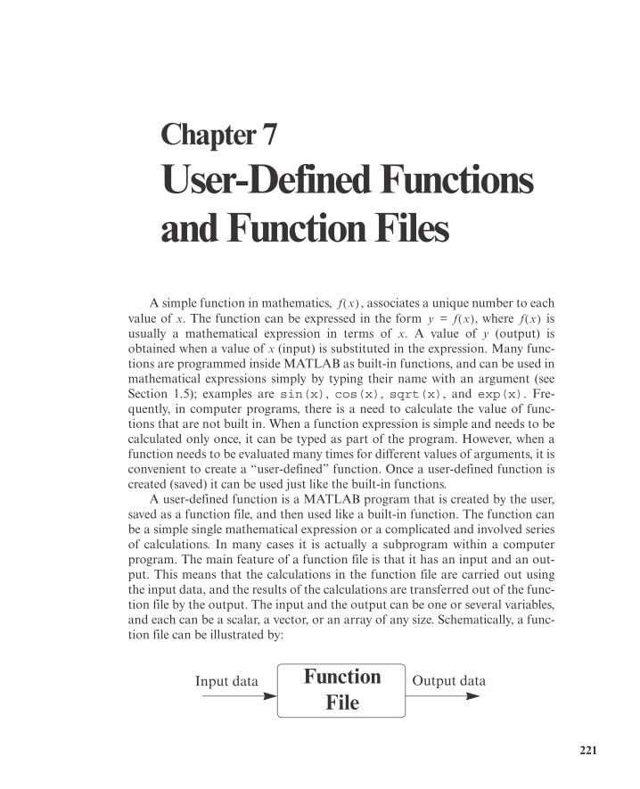
221
Chapter 7 User-Defined Functions and Function Files
A simple function in mathematics, , associates a unique number to eachvalue of x. The function can be expressed in the form , where isusually a mathematical expression in terms of x. A value of y (output) isobtained when a value of x (input) is substituted in the expression. Many func-tions are programmed inside MATLAB as built-in functions, and can be used inmathematical expressions simply by typing their name with an argument (seeSection 1.5); examples are sin(x), cos(x), sqrt(x), and exp(x). Fre-quently, in computer programs, there is a need to calculate the value of func-tions that are not built in. When a function expression is simple and needs to becalculated only once, it can be typed as part of the program. However, when afunction needs to be evaluated many times for different values of arguments, it isconvenient to create a “user-defined” function. Once a user-defined function iscreated (saved) it can be used just like the built-in functions.
A user-defined function is a MATLAB program that is created by the user,saved as a function file, and then used like a built-in function. The function canbe a simple single mathematical expression or a complicated and involved seriesof calculations. In many cases it is actually a subprogram within a computerprogram. The main feature of a function file is that it has an input and an out-put. This means that the calculations in the function file are carried out usingthe input data, and the results of the calculations are transferred out of the func-tion file by the output. The input and the output can be one or several variables,and each can be a scalar, a vector, or an array of any size. Schematically, a func-tion file can be illustrated by:
f xy f x= f x
Function File
Input data Output data

222 Chapter 7: User-Defined Functions and Function Files
A very simple example of a user-defined function is a function that calcu-lates the maximum height that a ball reaches when thrown upward with a cer-
tain velocity. For a velocity , the maximum height is given by ,
where g is the gravitational acceleration. In function form this can be written as
. In this case the input to the function is the velocity (a number),
and the output is the maximum height (a number). For example, in SI units (g =9.81 m/s2) if the input is 15 m/s, the output is 11.47 m.
In addition to being used as math functions, user-defined functions can beused as subprograms in large programs. In this way large computer programscan be made up of smaller “building blocks” that can be tested independently.Function files are similar to subroutines in Basic and Fortran, procedures inPascal, and functions in C.
The fundamentals of user-defined functions are explained in Sections 7.1through 7.7. In addition to user-defined functions that are saved in separatefunction files and called for use in a computer program, MATLAB provides anoption to define and use a user-defined math function within a computer pro-gram (not in a separate file). This can be done by using anonymous function,which is presented in Section 7.8. There are built-in and user-defined functionsthat have to be supplied with other functions when they are called. These func-tions, which in MATLAB are called function functions, are introduced in Sec-tion 7.9. The last two sections cover subfunctions and nested functions. Both aremethods for incorporating two or more user-defined functions in a single func-tion file.
7.1 CREATING A FUNCTION FILE
Function files are created and edited, like script files, in the Editor/DebuggerWindow. This window is opened from the Command Window. In the Toolstripselect New, then select Function. Once the Editor/Debugger Window opens, itlooks like that shown in Figure 7-1. The editor contains several pre-typed linesthat outline the structure of a function file. The first line is the function defini-tion line, which is followed by comments the describe the function. Next comesthe program (the empty lines 4 and 5 in Figure 7-1), and the last line is an endstatement, which is optional. The structure of a function file is described indetail in the next section.
Note: The Editor/Debugger Window can also be opened (as was describedin Chapter 1) by clicking on the New Script icon in the Toolstrip, or by clickingNew in the Toolstrip and then selecting Script from the menu that open. The
v0 hmax
Function File15 m/s 11.47 m

7.2 Structure of a Function File 223
window that opens is empty, without any pre-typed lines. In general, the Editor/Debugger Window can be used for writing a script file or a function file.
7.2 STRUCTURE OF A FUNCTION FILE
The structure of a typical complete function file is shown in Figure 7-2. Thisparticular function calculates the monthly payment and the total payment of aloan. The inputs to the function are the amount of the loan, the annual interestrate, and the duration of the loan (number of years). The output from the func-tion is the monthly payment and the total payment.
Figure 7-1: The Editor/Debugger Window.
Figure 7-2: Structure of a typical function file.
The first line in a function file mustbe the function definition line.
Function definition line.
The H1 line.
Help text.
Assignment of values to output arguments.
Function body(computer program).
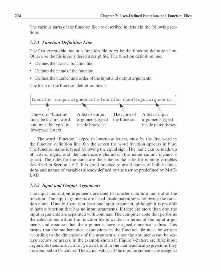
224 Chapter 7: User-Defined Functions and Function Files
The various parts of the function file are described in detail in the following sec-tions.
7.2.1 Function Definition Line
The first executable line in a function file must be the function definition line.Otherwise the file is considered a script file. The function definition line:
• Defines the file as a function file
• Defines the name of the function
• Defines the number and order of the input and output arguments
The form of the function definition line is:
The word “function,” typed in lowercase letters, must be the first word inthe function definition line. On the screen the word function appears in blue.The function name is typed following the equal sign. The name can be made upof letters, digits, and the underscore character (the name cannot include aspace). The rules for the name are the same as the rules for naming variablesdescribed in Section 1.6.2. It is good practice to avoid names of built-in func-tions and names of variables already defined by the user or predefined by MAT-LAB.
7.2.2 Input and Output Arguments
The input and output arguments are used to transfer data into and out of thefunction. The input arguments are listed inside parentheses following the func-tion name. Usually, there is at least one input argument, although it is possibleto have a function that has no input arguments. If there are more than one, theinput arguments are separated with commas. The computer code that performsthe calculations within the function file is written in terms of the input argu-ments and assumes that the arguments have assigned numerical values. Thismeans that the mathematical expressions in the function file must be writtenaccording to the dimensions of the arguments, since the arguments can be sca-lars, vectors, or arrays. In the example shown in Figure 7-2 there are three inputarguments (amount,rate,years), and in the mathematical expressions theyare assumed to be scalars. The actual values of the input arguments are assigned
function [output arguments] = function_name(input arguments)
The word “function” must be the first word, and must be typed in lowercase letters.
The name of the function.
A list of output arguments typed inside brackets.
A list of input arguments typed inside parentheses.

7.2 Structure of a Function File 225
when the function is used (called). Similarly, if the input arguments are vectorsor arrays, the mathematical expressions in the function body must be written tofollow linear algebra or element-by-element calculations.
The output arguments, which are listed inside brackets on the left side of theassignment operator in the function definition line, transfer the output from thefunction file. Function files can have zero, one, or several output arguments. Ifthere are more than one, the output arguments are separated with commas. Ifthere is only one output argument, it can be typed without brackets. For thefunction file to work, the output arguments must be assigned values in thecomputer program that is in the function body. In the example in Figure 7-2there are two output arguments, mpay and tpay. When a function does nothave an output argument, the assignment operator in the function definitionline can be omitted. A function without an output argument can, for example,generate a plot or write data to a file.
It is also possible to transfer strings into a function file. This is done by typ-ing the string as part of the input variables (text enclosed in single quotes).Strings can be used to transfer names of other functions into the function file.
Usually, all the input to, and the output from, a function file transferredthrough the input and output arguments. In addition, however, all the input andoutput features of script files are valid and can be used in function files. Thismeans that any variable that is assigned a value in the code of the function filewill be displayed on the screen unless a semicolon is typed at the end of the com-mand. In addition, the input command can be used to input data interactively,and the disp, fprintf, and plot commands can be used to display informa-tion on the screen, save to a file, or plot figures just as in a script file. The follow-ing are examples of function definition lines with different combinations ofinput and output arguments.
Function definition line Comments
function[mpay,tpay]= loan(amount,rate,years) Three input arguments, twooutput arguments.
function [A] = RectArea(a,b) Two input arguments, one out-put argument.
function A = RectArea(a,b) Same as above; one outputargument can be typed with-out the brackets.
function [V, S] = SphereVolArea(r) One input variable, two outputvariables.
function trajectory(v,h,g) Three input arguments, nooutput arguments.

226 Chapter 7: User-Defined Functions and Function Files
7.2.3 The H1 Line and Help Text Lines
The H1 line and help text lines are comment lines (lines that begin with the per-cent, %, sign) following the function definition line. They are optional but arefrequently used to provide information about the function. The H1 line is thefirst comment line and usually contains the name and a short definition of thefunction. When a user types (in the Command Window) lookfor a_word,MATLAB searches for a_word in the H1 lines of all the functions, and if amatch is found, the H1 line that contains the match is displayed.
The help text lines are comment lines that follow the H1 line. These linescontain an explanation of the function and any instructions related to the inputand output arguments. The comment lines that are typed between the functiondefinition line and the first non-comment line (the H1 line and the help text) aredisplayed when the user types help function_name in the Command Win-dow. This is true for MATLAB built-in functions as well as the user-definedfunctions. For example, for the function loan in Figure 7-2, if help loan istyped in the Command Window (make sure the current directory or the searchpath includes the directory where the file is saved), the display on the screen is:
A function file can include additional comment lines in the function body. Theselines are ignored by the help command.
7.2.4 Function Body
The function body contains the computer program (code) that actually per-forms the computations. The code can use all MATLAB programming features.This includes calculations, assignments, any built-in or user-defined functions,flow control (conditional statements and loops) as explained in Chapter 6, com-ments, blank lines, and interactive input and output.
7.3 LOCAL AND GLOBAL VARIABLES
All the variables in a function file are local (the input and output arguments andany variables that are assigned values within the function file). This means thatthe variables are defined and recognized only inside the function file. When a
>> help loan
loan calculates monthly and total payment of loan.
Input arguments:
amount=loan amount in $.
rate=annual interest rate in percent.
years=number of years.
Output arguments:
mpay=monthly payment, tpay=total payment.

7.4 Saving a Function File 227
function file is executed, MATLAB uses an area of memory that is separatefrom the workspace (the memory space of the Command Window and the scriptfiles). In a function file the input variables are assigned values each time thefunction is called. These variables are then used in the calculations within thefunction file. When the function file finishes its execution, the values of the out-put arguments are transferred to the variables that were used when the functionwas called. All this means that a function file can have variables with the samenames as variables in the Command Window or in script files. The function filedoes not recognize variables with the same names as have been assigned valuesoutside the function. The assignment of values to these variables in the functionfile will not change their assignment elsewhere.
Each function file has its own local variables, which are not shared withother functions or with the workspace of the Command Window and the scriptfiles. It is possible, however, to make a variable common (recognized) in severaldifferent function files, and perhaps in the workspace too. This is done bydeclaring the variable global with the global command, which has the form:
Several variables can be declared global by listing them, separated with spaces,in the global command. For example:
global GRAVITY_CONST FrictionCoefficient
• The variable has to be declared global in every function file that the user wants itto be recognized in. The variable is then common only to these files.
• The global command must appear before the variable is used. It is recom-mended to enter the global command at the top of the file.
• The global command has to be entered in the Command Window, or in ascript file, for the variable to be recognized in the workspace.
• The variable can be assigned, or reassigned, a value in any of the locations inwhich it is declared common.
• The use of long descriptive names (or all capital letters) is recommended forglobal variables in order to distinguish them from regular variables.
7.4 SAVING A FUNCTION FILE
A function file must be saved before it can be used. This is done, as with a scriptfile, by choosing Save as . . . from the File menu, selecting a location (many stu-dents save to a flash drive), and entering the file name. It is highly recommendedthat the file be saved with a name that is identical to the function name in thefunction definition line. In this way the function is called (used) by using thefunction name. (If a function file is saved with a different name, the name it issaved under must be used when the function is called.) Function files are saved
global variable_name

228 Chapter 7: User-Defined Functions and Function Files
with the extension .m. Examples:
7.5 USING A USER-DEFINED FUNCTION
A user-defined function is used in the same way as a built-in function. The func-tion can be called from the Command Window, from a script file, or fromanother function. To use the function file, the folder where it is saved must eitherbe in the current folder or be in the search path (see Sections 1.8.3 and 1.8.4).
A function can be used by assigning its output to a variable (or variables), asa part of a mathematical expression, as an argument in another function, or justby typing its name in the Command Window or in a script file. In all cases theuser must know exactly what the input and output arguments are. An inputargument can be a number, a computable expression, or a variable that has anassigned value. The arguments are assigned according to their position in theinput and output argument lists in the function definition line.
Two of the ways that a function can be used are illustrated below with theuser-defined loan function in Figure 7-2, which calculates the monthly andtotal payments (two output arguments) of a loan. The input arguments are theloan amount, annual interest rate, and the length (number of years) of the loan.In the first illustration the loan function is used with numbers as input argu-ments:
In the second illustration the loan function is used with two pre-assignedvariables and a number as the input arguments:
Function definition line File name
function [mpay,tpay] = loan(amount,rate,years) loan.m
function [A] = RectArea(a,b) RectArea.m
function [V, S] = SphereVolArea(r) SphereVolArea.m
function trajectory(v,h,g) trajectory.m
>> [month total]=loan(25000,7.5,4)
month = 600.72total = 28834.47
>> a=70000; b=6.5;
>> [x y]=loan(a,b,30)
First argument is loan amount, second is interest rate, and third is number of years.
Define variables a and b.
Use a, b, and the number 30 for inputarguments and x (monthly pay) and y(total pay) for output arguments.

7.6 Examples of Simple User-Defined Functions 229
7.6 EXAMPLES OF SIMPLE USER-DEFINED FUNCTIONS
Sample Problem 7-1: User-defined function for a math function
Write a function file (name it chp7one) for the function . The
input to the function is x and the output is . Write the function such that xcan be a vector. Use the function to calculate:(a) for x = 6.(b) for x = 1, 3, 5, 7, 9, and 11.
Solution
The function file for the function is:
Note that the mathematical expression in the function file is written for element-by-element calculations. In this way if x is a vector, y will also be a vector. Thefunction is saved and then the search path is modified to include the directorywhere the file was saved. As shown below, the function is used in the CommandWindow.(a) Calculating the function for can be done by typing chp7one(6) inthe Command Window, or by assigning the value of the function to a new vari-able:
(b) To calculate the function for several values of x, a vector with the values of xis created and then used for the argument of the function.
x = 440.06y = 158423.02
function y=chp7one(x)
y=(x.^4.*sqrt(3*x+5))./(x.^2+1).^2;
>> chp7one(6)
ans = 4.5401
>> F=chp7one(6)
F = 4.5401
>> x=1:2:11
x = 1 3 5 7 9 11
f x
f xf x
f x
Function definition line.
Assignment to output argument.
x 6=
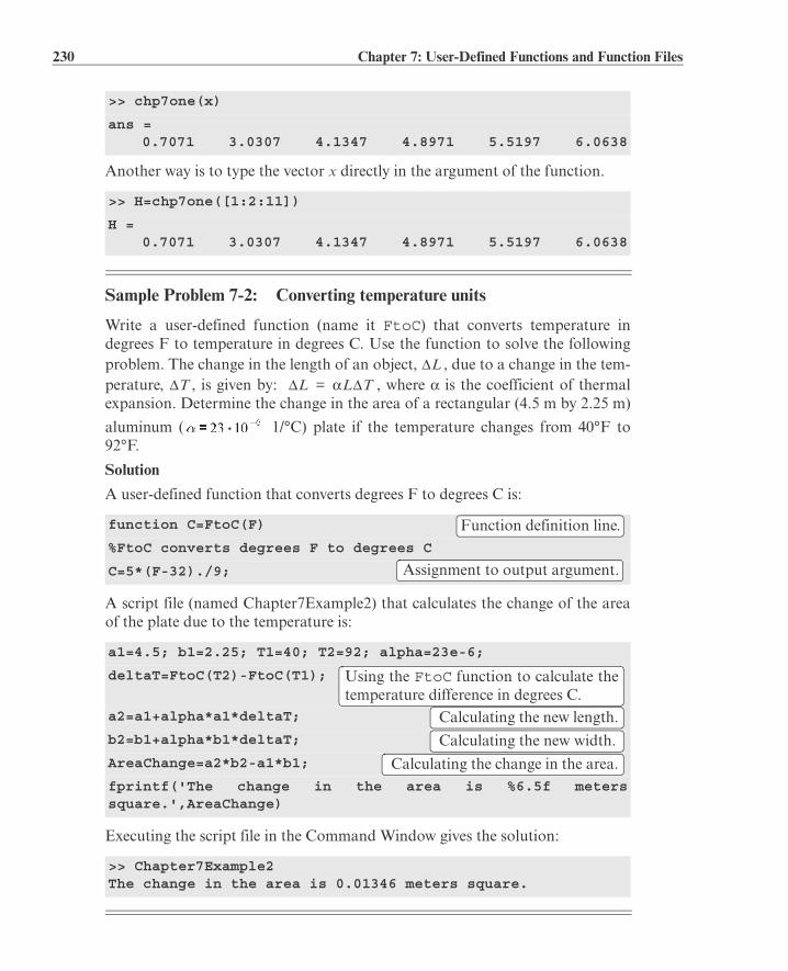
230 Chapter 7: User-Defined Functions and Function Files
Another way is to type the vector x directly in the argument of the function.
Sample Problem 7-2: Converting temperature units
Write a user-defined function (name it FtoC) that converts temperature indegrees F to temperature in degrees C. Use the function to solve the followingproblem. The change in the length of an object, , due to a change in the tem-perature, , is given by: , where is the coefficient of thermalexpansion. Determine the change in the area of a rectangular (4.5 m by 2.25 m)
aluminum ( 1/°C) plate if the temperature changes from 40°F to92°F.
Solution
A user-defined function that converts degrees F to degrees C is:
A script file (named Chapter7Example2) that calculates the change of the areaof the plate due to the temperature is:
Executing the script file in the Command Window gives the solution:
>> chp7one(x)
ans = 0.7071 3.0307 4.1347 4.8971 5.5197 6.0638
>> H=chp7one([1:2:11])
H = 0.7071 3.0307 4.1347 4.8971 5.5197 6.0638
function C=FtoC(F)
%FtoC converts degrees F to degrees C
C=5*(F-32)./9;
a1=4.5; b1=2.25; T1=40; T2=92; alpha=23e-6;
deltaT=FtoC(T2)-FtoC(T1);
a2=a1+alpha*a1*deltaT;
b2=b1+alpha*b1*deltaT;
AreaChange=a2*b2-a1*b1;
fprintf('The change in the area is %6.5f meterssquare.',AreaChange)
>> Chapter7Example2The change in the area is 0.01346 meters square.
LT L L T=
Function definition line.
Assignment to output argument.
Using the FtoC function to calculate thetemperature difference in degrees C.
Calculating the new length.
Calculating the new width.
Calculating the change in the area.

7.7 Comparison between Script Files and Function Files 231
7.7 COMPARISON BETWEEN SCRIPT FILES AND FUNCTION FILES
Students who are studying MATLAB for the first time sometimes have difficultyunderstanding exactly the differences between script and function files, since formany of the problems that they are asked to solve using MATLAB, either typeof file can be used. The similarities and differences between script and functionfiles are summarized below.
• Both script and function files are saved with the extension .m (that is why theyare sometimes called M-files).
• The first executable line in a function file is (must be) the function definition line.
• The variables in a function file are local. The variables in a script file are recog-nized in the Command Window.
• Script files can use variables that have been defined in the workspace.
• Script files contain a sequence of MATLAB commands (statements).
• Function files can accept data through input arguments and can return datathrough output arguments.
• When a function file is saved, the name of the file should be the same as thename of the function.
• A user-defined function is used in the same way as a built-in function. It can beused (called) in the Command Window, in a script file, or in another function.
7.8 ANONYMOUS FUNCTIONS
User-defined functions written in function files can be used for simple mathe-matical functions, for large and complicated math functions that require exten-sive programming, and as subprograms in large computer programs. In caseswhen the value of a relatively simple mathematical expression has to be calcu-lated many times within a program, MATLAB provides the option of usinganonymous functions. An anonymous function is a user-defined function that isdefined and written within the computer code (not in a separate function file)and is then used in the code. Anonymous functions can be defined in any part ofMATLAB (in the Command Window, in script files, and inside regular user-defined functions).
An anonymous function is a simple (one-line) user-defined function that isdefined without creating a separate function file (m-file). Anonymous functionscan be constructed in the Command Window, within a script file, or inside a reg-ular user-defined function.

232 Chapter 7: User-Defined Functions and Function Files
An anonymous function is created by typing the following command:
A simple example is cube = @ (x) x^3, which calculates the cube of the inputargument.• The command creates the anonymous function and assigns a handle for the
function to the variable name on the left-hand side of the = sign. (Function han-dles provide means for using the function and passing it to other functions; seeSection 7.9.1.)
• The expr consists of a single valid mathematical MATLAB expression.
• The mathematical expression can have one or several independent variables. Theindependent variable(s) is (are) entered in the (arglist). Multiple indepen-dent variables are separated with commas. An example of an anonymous func-tion that has two independent variables is: circle = @ (x,y)16*x^2+9*y^2.
• The mathematical expression can include any built-in or user-defined functions.
• The expression must be written according to the dimensions of the arguments(element-by-element or linear algebra calculations).
• The expression can include variables that are already defined when the anony-mous function is defined. For example, if three variables a, b, and c are defined(have assigned numerical values), then they can be used in the expression of theanonymous function parabola = @ (x) a*x^2+b*x+c.
Important note: MATLAB captures the values of the predefined variableswhen the anonymous function is defined. This means that if new values are sub-sequently assigned to the predefined variables, the anonymous function is notchanged. The anonymous function has to be redefined in order for the new val-ues of the predefined variables to be used in the expression.
Using an anonymous function:
• Once an anonymous function is defined, it can be used by typing its name and avalue for the argument (or arguments) in parentheses (see examples that follow).
• Anonymous functions can also be used as arguments in other functions (see Sec-tion 7.9.1).
name = @ (arglist) expr
The name of the anon-ymous function.
The @ symbol.
A list of input argu-ments (indepen-dent variables).
Mathematical expression.

7.8 Anonymous Functions 233
Example of an anonymous function with one independent variable:
The function can be defined (in the Command Window) as an
anonymous function for x as a scalar by:
If a semicolon is not typed at the end, MATLAB responds by displaying thefunction. The function can then be used for different values of x, as shownbelow.
If x is expected to be an array, with the function calculated for each element,then the function must be modified for element-by-element calculations.
Example of an anonymous function with several independent variables:
The function can be defined as an anonymous functionby:
Then the anonymous function can be used for different values of x and y. Forexample, typing HA(2,3) gives:
>> FA = @ (x) exp(x^2)/sqrt(x^2+5)
FA = @(x)exp(x^2)/sqrt(x^2+5)
>> FA(2)
ans = 18.1994
>> z = FA(3)
z = 2.1656e+003
>> FA = @ (x) exp(x.^2)./sqrt(x.^2+5)
FA = @(x)exp(x.^2)./sqrt(x.^2+5)
>> FA([1 0.5 2])ans = 1.1097 0.5604 18.1994
>> HA = @ (x,y) 2*x^2 - 4*x*y + y^2
HA = @(x,y)2*x^2-4*x*y+y^2
>> HA(2,3)ans = -7
Using a vector as input argument.
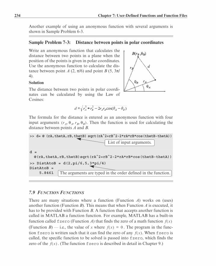
234 Chapter 7: User-Defined Functions and Function Files
Another example of using an anonymous function with several arguments isshown in Sample Problem 6-3.
Sample Problem 7-3: Distance between points in polar coordinates
Write an anonymous function that calculates thedistance between two points in a plane when theposition of the points is given in polar coordinates.Use the anonymous function to calculate the dis-tance between point A (2, /6) and point B (5, 3 /4).
Solution
The distance between two points in polar coordi-nates can be calculated by using the Law ofCosines:
The formula for the distance is entered as an anonymous function with fourinput arguments . Then the function is used for calculating thedistance between points A and B.
7.9 FUNCTION FUNCTIONS
There are many situations where a function (Function A) works on (uses)another function (Function B). This means that when Function A is executed, ithas to be provided with Function B. A function that accepts another function iscalled in MATLAB a function function. For example, MATLAB has a built-infunction called fzero (Function A) that finds the zero of a math function (Function B) — i.e., the value of x where . The program in the func-tion fzero is written such that it can find the zero of any . When fzero iscalled, the specific function to be solved is passed into fzero, which finds thezero of the . (The function fzero is described in detail in Chapter 9.)
>> d= @ (rA,thetA,rB,thetB) sqrt(rA^2+rB^2-2*rA*rB*cos(thetB-thetA))
d = @(rA,thetA,rB,thetB)sqrt(rA^2+rB^2-2*rA*rB*cos(thetB-thetA))
>> DistAtoB = d(2,pi/6,5,3*pi/4)DistAtoB = 5.8461
rA A rB B, , ,
List of input arguments.
The arguments are typed in the order defined in the function.
f x
f x 0=f x
f x

7.9 Function Functions 235
A function function, which accepts another function (imported function),includes in its input arguments a name that represents the imported function.The imported function name is used for the operations in the program (code) ofthe function function. When the function function is used (called), the specificfunction that is imported is listed in its input argument. In this way differentfunctions can be imported (passed) into the function function. There are twomethods for listing the name of an imported function in the argument list of afunction function. One is by using a function handle (Section 7.9.1), and theother is by typing the name of the function that is being passed in as a stringexpression (Section 7.9.2). The method that is used affects the way that the oper-ations in the function function are written (this is explained in more detail in thenext two sections). Using function handles is easier and more efficient, andshould be the preferred method.
7.9.1 Using Function Handles for Passing a Function into a Function Function
Function handles are used for passing (importing) user-defined functions, built-in functions, and anonymous functions into function functions that can acceptthem. This section first explains what a function handle is, then shows how towrite a user-defined function function that accepts function handles, and finallyshows how to use function handles for passing functions into function func-tions.
Function handle:
A function handle is a MATLAB value that is associated with a function. It is aMATLAB data type and can be passed as an argument into another function.Once passed, the function handle provides means for calling (using) the func-tion it is associated with. Function handles can be used with any kind of MAT-LAB function. This includes built-in functions, user-defined functions (writtenin function files), and anonymous functions.• For built-in and user-defined functions, a function handle is created by typing
the symbol @ in front of the function name. For example, @cos is the functionhandle of the built-in function cos, and @FtoC is the function handle of theuser-defined function FtoC that was created in Sample Problem 7-2.
• The function handle can also be assigned to a variable name. For example,cosHandle=@cos assigns the handle @cos to cosHandle. Then the namecosHandle can be used for passing the handle.
• As anonymous functions (see Section 7.8.1), their name is already a functionhandle.
Writing a function function that accepts a function handle as an input argument:
As already mentioned, the input arguments of a function function (whichaccepts another function) includes a name (dummy function name) that rep-
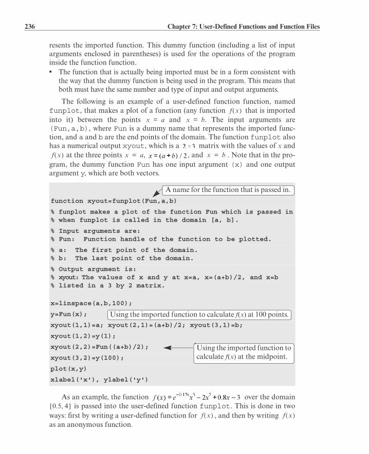
236 Chapter 7: User-Defined Functions and Function Files
resents the imported function. This dummy function (including a list of inputarguments enclosed in parentheses) is used for the operations of the programinside the function function.• The function that is actually being imported must be in a form consistent with
the way that the dummy function is being used in the program. This means thatboth must have the same number and type of input and output arguments.
The following is an example of a user-defined function function, namedfunplot, that makes a plot of a function (any function that is importedinto it) between the points and . The input arguments are(Fun,a,b), where Fun is a dummy name that represents the imported func-tion, and a and b are the end points of the domain. The function funplot alsohas a numerical output xyout, which is a matrix with the values of x and
at the three points , , and . Note that in the pro-gram, the dummy function Fun has one input argument (x) and one outputargument y, which are both vectors.
As an example, the function over the domain is passed into the user-defined function funplot. This is done in two
ways: first by writing a user-defined function for , and then by writing as an anonymous function.
function xyout=funplot(Fun,a,b)
% funplot makes a plot of the function Fun which is passed in% when funplot is called in the domain [a, b].
% Input arguments are:% Fun: Function handle of the function to be plotted.
% a: The first point of the domain.% b: The last point of the domain.
% Output argument is:% xyout: The values of x and y at x=a, x=(a+b)/2, and x=b% listed in a 3 by 2 matrix.
x=linspace(a,b,100);
y=Fun(x);
xyout(1,1)=a; xyout(2,1)=(a+b)/2; xyout(3,1)=b;
xyout(1,2)=y(1);
xyout(2,2)=Fun((a+b)/2);
xyout(3,2)=y(100);
plot(x,y)
xlabel('x'), ylabel('y')
f xx a= x b=
f x x a= x b=
A name for the function that is passed in.
Using the imported function to calculate f(x) at 100 points.
Using the imported function to calculate f(x) at the midpoint.
0.5 4,f x f x

7.9 Function Functions 237
Passing a user-defined function into a function function:
First, a user-defined function is written for . The function, named Fdemo,calculates for a given value of x and is written using element-by-elementoperations.
Next, the function Fdemo is passed into the user-defined function functionfunplot, which is called in the Command Window. Note that a handle of theuser-defined function Fdemo is entered (the handle is @Fdemo) for the inputargument Fun in the user-defined function funplot.
In addition to the display of the numerical output, when the command isexecuted, the plot shown in Figure 7-3 is displayed in the Figure Window.
Passing an anonymous function into a function function:
To use an anonymous function, the function firsthas to be written as an anonymous function, and then passed into the user-defined function funplot. The following shows how both of these steps aredone in the Command Window. Note that the name of the anonymous functionFdemoAnony is entered without the @ sign for the input argument Fun in theuser-defined function funplot (since the name is already the handle of theanonymous function).
function y=Fdemo(x)y=exp(-0.17*x).*x.^3-2*x.^2+0.8*x-3;
>> ydemo=funplot(@Fdemo,0.5,4)ydemo = 0.5000 -2.9852 2.2500 -3.5548 4.0000 0.6235
Figure 7-3: A plot of the function .
f x
f x
Enter a handle of the user-defined function Fdemo.
x0.5 1 1.5 2 2.5 3 3.5 4
f(x)
-4
-3
-2
-1
0
1

238 Chapter 7: User-Defined Functions and Function Files
In addition to the display of the numerical output in the Command Window,the plot shown in Figure 7-3 is displayed in the Figure Window.
7.9.2 Using a Function Name for Passing a Function into a Function Function
A second method for passing a function into a function function is by typing thename of the function that is being imported as a string in the input argument ofthe function function. The method that was used before the introduction offunction handles can be used for importing user-defined functions. As men-tioned, function handles are easier to use and more efficient and should be thepreferred method. Importing user-defined functions by using their name is cov-ered in the present edition of the book for the benefit of readers who need tounderstand programs written before MATLAB 7. New programs should usefunction handles.
When a user-defined function is imported by using its name, the value of theimported function inside the function function has to be calculated with thefeval command. This is different from the case where a function handle isused, which means that there is a difference in the way that the code in the func-tion function is written that depends on how the imported function is passed in.
The feval command:
The feval (short for “function evaluate”) command evaluates the value of afunction for a given value (or values) of the function’s argument (or arguments).The format of the command is:
The value that is determined by feval can be assigned to a variable, or if thecommand is typed without an assignment, MATLAB displays ans = and thevalue of the function.
• The function name is typed as string.
• The function can be a built-in or a user-defined function.
• If there is more than one input argument, the arguments are separated withcommas.
>> FdemoAnony=@(x) exp(-0.17*x).*x.^3-2*x.^2+0.8*x-3FdemoAnony = @(x) exp(-0.17*x).*x.^3-2*x.^2+0.8*x-3
>> ydemo=funplot(FdemoAnony,0.5,4)
ydemo = 0.5000 -2.9852 2.2500 -3.5548 4.0000 0.6235
Create an anonymous function for .f x
Enter the name of the anony-mous function (FdemoAnony).
variable = feval(‘function name’, argument value)

7.9 Function Functions 239
• If there is more than one output argument, the variables on the left-hand side ofthe assignment operator are typed inside brackets and separated with commas.
Two examples using the feval command with built-in functions follow.
The following shows the use of the feval command with the user-definedfunction loan that was created earlier in the chapter (Figure 7-2). This functionhas three input arguments and two output arguments.
Writing a function function that accepts a function by typing its name as an inputargument:
As already mentioned, when a user-defined function is imported by using itsname, the value of the function inside the function function has to be calculatedwith the feval command. This is demonstrated in the following user-definedfunction function that is called funplotS. The function is the same as thefunction funplot from Section 7.9.1, except that the command feval is usedfor the calculations with the imported function.
>> feval('sqrt',64)
ans = 8
>> x=feval('sin',pi/6)
x = 0.5000
>> [M,T]=feval('loan',50000,3.9,10)
M = 502.22
T = 60266.47
function xyout=funplotS(Fun,a,b)
% funplotS makes a plot of the function Fun which is passedin% when funplotS is called in the domain [a, b].
% Input arguments are:% Fun: The function to be plotted. Its name is entered asstring expression.
% a: The first point of the domain.% b: The last point of the domain.
A $50,000 loan, 3.9% interest, 10 years.
Monthly payment.
Total payment.
A name for the function that is passed in.

240 Chapter 7: User-Defined Functions and Function Files
Passing a user-defined function into another function by using a string expression:
The following demonstrates how to pass a user-defined function into a functionfunction by typing the name of the imported function as a string in the input
argument. The function from Section 7.9.1, cre-ated as a user-defined function named Fdemo, is passed into the user-definedfunction funplotS. Note that the name Fdemo is typed in a string for theinput argument Fun in the user-defined function funplotS.
In addition to the display of the numerical output in the Command Window,the plot shown in Figure 7-3 is displayed in the Figure Window.
7.10 SUBFUNCTIONS
A function file can contain more than one user-defined function. The functionsare typed one after the other. Each function begins with a function definitionline. The first function is called the primary function and the rest of the func-tions are called subfunctions. The subfunctions can be typed in any order. Thename of the function file that is saved should correspond to the name of the pri-mary function. Each of the functions in the file can call any of the other func-tions in the file. Outside functions, or programs (script files), can call only theprimary function. Each of the functions in the file has its own workspace, whichmeans that in each the variables are local. In other words, the primary functionand the subfunctions cannot access each other’s variables (unless variables are
% Output argument is:% xyout: The values of x and y at x=a, x=(a+b)/2, and x=b% listed in a 3 by 2 matrix.
x=linspace(a,b,100);
y=feval(Fun,x);
xyout(1,1)=a; xyout(2,1)=(a+b)/2; xyout(3,1)=b;
xyout(1,2)=y(1);
xyout(2,2)=feval(Fun,(a+b)/2);
xyout(3,2)=y(100);
plot(x,y)
xlabel('x'), ylabel('y')
>> ydemoS=funplotS('Fdemo',0.5,4)
ydemoS = 0.5000 -2.9852 2.2500 -3.5548 4.0000 0.6235
Using the imported function to calculate f(x) at 100 points.
Using the imported function to calculate f(x) at the midpoint.
The name of the imported function is typed as a string.

7.10 Subfunctions 241
declared to be global). Subfunctions can help in writing user-defined functions in an organized
manner. The program in the primary function can be divided into smaller tasks,each of which is carried out in a subfunction. This is demonstrated in SampleProblem 7-4.
Sample Problem 7-4: Average and standard deviation
Write a user-defined function that calculates the average and the standard devia-tion of a list of numbers. Use the function to calculate the average and the stan-dard deviation of the following list of grades:80 75 91 60 79 89 65 80 95 50 81
Solution
The average (mean) of a given set of n numbers is given by:
The standard deviation is given by:
A user-defined function, named stat, is written for solving the problem. Todemonstrate the use of subfunctions, the function file includes stat as a pri-mary function, and two subfunctions called AVG and StandDiv. The functionAVG calculates , and the function StandDiv calculates . The subfunc-tions are called by the primary function.The following listing is saved as onefunction file called stat.
The user-defined function stat is then used in the Command Window for cal-culating the average and the standard deviation of the grades:
function [me SD] = stat(v)
n=length(v);
me=AVG(v,n);
SD=StandDiv(v,me,n);
function av=AVG(x,num)
av=sum(x)/num;
function Sdiv=StandDiv(x,xAve,num)
xdif=x-xAve;
xdif2=xdif.^2;
Sdiv= sqrt(sum(xdif2)/(num-1));
xave x1 x2 xn, , ,
xave
The primary function.
Subfunction.
Subfunction.

242 Chapter 7: User-Defined Functions and Function Files
7.11 NESTED FUNCTIONS
A nested function is a user-defined function that is written inside another user-defined function. The portion of the code that corresponds to the nested func-tion starts with a function definition line and ends with an end statement. Anend statement must also be entered at the end of the function that contains thenested function. (Normally, a user-defined function does not require a terminat-ing end statement. However, an end statement is required if the function con-tains one or more nested functions.) Nested functions can also contain nestedfunctions. Obviously, having many levels of nested functions can be confusing.This section considers only two levels of nested functions.
One nested function:
The format of a user-defined function A (called the primary function) that con-tains one nested function B is:
function y=A(a1,a2).......
function z=B(b1,b2).......end
.......end
• Note the end statements at the ends of functions B and A.
• The nested function B can access the workspace of the primary function A, andthe primary function A can access the workspace of the function B. This meansthat a variable defined in the primary function A can be read and redefined innested function B and vice versa.
• Function A can call function B, and function B can call function A.
Two (or more) nested functions at the same level:
The format of a user-defined function A (called the primary function) that con-tains two nested functions B and C at the same level is:
>> Grades=[80 75 91 60 79 89 65 80 95 50 81];
>> [AveGrade StanDeviation] = stat(Grades)
AveGrade = 76.8182
StanDeviation = 13.6661
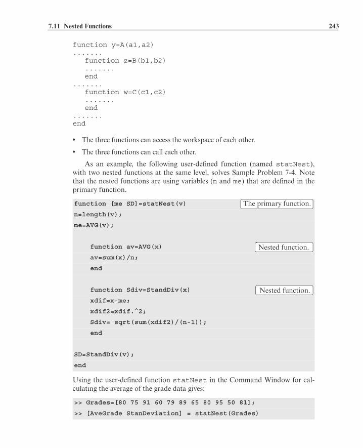
7.11 Nested Functions 243
function y=A(a1,a2).......
function z=B(b1,b2).......end
.......function w=C(c1,c2).......end
.......end
• The three functions can access the workspace of each other.
• The three functions can call each other.
As an example, the following user-defined function (named statNest),with two nested functions at the same level, solves Sample Problem 7-4. Notethat the nested functions are using variables (n and me) that are defined in theprimary function.
Using the user-defined function statNest in the Command Window for cal-culating the average of the grade data gives:
function [me SD]=statNest(v)
n=length(v);
me=AVG(v);
function av=AVG(x)
av=sum(x)/n;
end
function Sdiv=StandDiv(x)
xdif=x-me;
xdif2=xdif.^2;
Sdiv= sqrt(sum(xdif2)/(n-1));
end
SD=StandDiv(v);
end
>> Grades=[80 75 91 60 79 89 65 80 95 50 81];
>> [AveGrade StanDeviation] = statNest(Grades)
The primary function.
Nested function.
Nested function.

244 Chapter 7: User-Defined Functions and Function Files
Two levels of nested functions:
Two levels of nested functions are created when nested functions are writteninside nested functions. The following shows an example for the format of auser-defined function with four nested functions in two levels.
function y=A(a1,a2) (Primary function A.).......
function z=B(b1,b2) (B is nested function in A.).......
function w=C(c1,c2) (C is nested function in B.).......end
endfunction u=D(d1,d2) (D is nested function in A.).......
function h=E(e1,e2) (E is nested function in D.).......end
end.......end
The following rules apply to nested functions:• A nested function can be called from a level above it. (In the preceding example,
function A can call B or D, but not C or E.)
• A nested function can be called from a nested function at the same level withinthe primary function. (In the preceding example, function B can call D, and Dcan call B.)
• A nested function can be called from a nested function at any lower level.
• A variable defined in the primary function is recognized and can be redefined bya function that is nested at any level within the primary function.
• A variable defined in a nested function is recognized and can be redefined by anyof the functions that contain the nested function.
AveGrade = 76.8182
StanDeviation = 13.6661

7.12 Examples of MATLAB Applications 245
7.12 EXAMPLES OF MATLAB APPLICATIONS
Sample Problem 7-5: Exponential growth and decay
A model for exponential growth or decay of a quantity is given by
where and are the quantity at time t and time 0, respectively, and k is aconstant unique to the specific application.
Write a user-defined function that uses this model to predict the quantity at time t from knowledge of and at some other time . For func-
tion name and arguments, use At = expGD(A0,At1,t1,t), where the outputargument At corresponds to , and for input arguments, useA0,At1,t1,t, corresponding to , , , and t, respectively.
Use the function file in the Command Window for the following two cases:(a) The population of Mexico was 67 million in the year 1980 and 79 million in
1986. Estimate the population in 2000.(b) The half-life of a radioactive material is 5.8 years. How much of a 7-gram
sample will be left after 30 years?
Solution
To use the exponential growth model, the value of the constant k has to bedetermined first by solving for k in terms of , , and :
Once k is known, the model can be used to estimate the population at any time.The user-defined function that solves the problem is:
function At=expGD(A0,At1,t1,t)
% expGD calculates exponential growth and decay
% Input arguments are:
% A0: Quantity at time zero.
% At1: Quantity at time t1.
% t1: The time t1.
% t: time t.
% Output argument is:
% At: Quantity at time t.
k=log(At1/A0)/t1;
At=A0*exp(k*t);
A t A0ekt=
A t A0
A t A0 A t1 t1
A tA0 A t1 t1
A0 A t1 t1
Function definition line.
Determination of k.
Determination of A(t).(Assignment of value to output variable.)

246 Chapter 7: User-Defined Functions and Function Files
Once the function is saved, it is used in the Command Window to solve the twocases. For case a) , , , and :
For case b) , (since corresponds to the half-life, which isthe time required for the material to decay to half of its initial quantity),
, and .
Sample Problem 7-6: Motion of a projectile
Create a function file that calculates thetrajectory of a projectile. The inputs to thefunction are the initial velocity and theangle at which the projectile is fired. Theoutputs from the function are the maxi-mum height and distance. In addition, thefunction generates a plot of the trajectory.Use the function to calculate the trajectory of a projectile that is fired at a veloc-ity of 230 m/s at an angle of 39°.
Solution
The motion of a projectile can be analyzed by considering the horizontal andvertical components. The initial velocity can be resolved into horizontal andvertical components
and
In the vertical direction the velocity and position of the projectile are given by:
and
The time it takes the projectile to reach the highest point and the corre-sponding height are given by:
and
The total flying time is twice the time it takes the projectile to reach the highestpoint, . In the horizontal direction the velocity is constant, and theposition of the projectile is given by:
>> expGD(67,79,6,20)ans = 116.03
>> expGD(7,3.5,5.8,30)ans = 0.19
A0 67= A t1 79= t1 6= t 20=
Estimation of the population in the year 2000.
A0 7= A t1 3.5= t1
t1 5.8= t 30=
The amount of material after 30 years.
v0
v0x v0 cos= v0y v0 sin=
vy 0=
ttot 2thmax=
x v0xt=

7.12 Examples of MATLAB Applications 247
In MATLAB notation the function name and arguments are entered as[hmax,dmax] = trajectory(v0,theta). The function file is:
After the function is saved, it is used in the Command Window for a projec-tile that is fired at a velocity of 230 m/s and an angle of 39°.
function [hmax,dmax]=trajectory(v0,theta)
% trajectory calculates the max height and distance of aprojectile, and makes a plot of the trajectory.
% Input arguments are:
% v0: initial velocity in (m/s).
% theta: angle in degrees.
% Output arguments are:
% hmax: maximum height in (m).
% dmax: maximum distance in (m).
% The function creates also a plot of the trajectory.
g=9.81;
v0x=v0*cos(theta*pi/180);
v0y=v0*sin(theta*pi/180);
thmax=v0y/g;
hmax=v0y^2/(2*g);
ttot=2*thmax;
dmax=v0x*ttot;
% Creating a trajectory plot
tplot=linspace(0,ttot,200);
x=v0x*tplot;
y=v0y*tplot-0.5*g*tplot.^2;
plot(x,y)
xlabel('DISTANCE (m)')
ylabel('HEIGHT (m)')
title('PROJECTILE''S TRAJECTORY')
>> [h d]=trajectory(230,39)
h = 1.0678e+003
d = 5.2746e+003
Function definition line.
Creating a time vector with 200 elements.
Calculating the x and y coordi-nates of the projectile at each time.
Note the element-by-element multiplication.
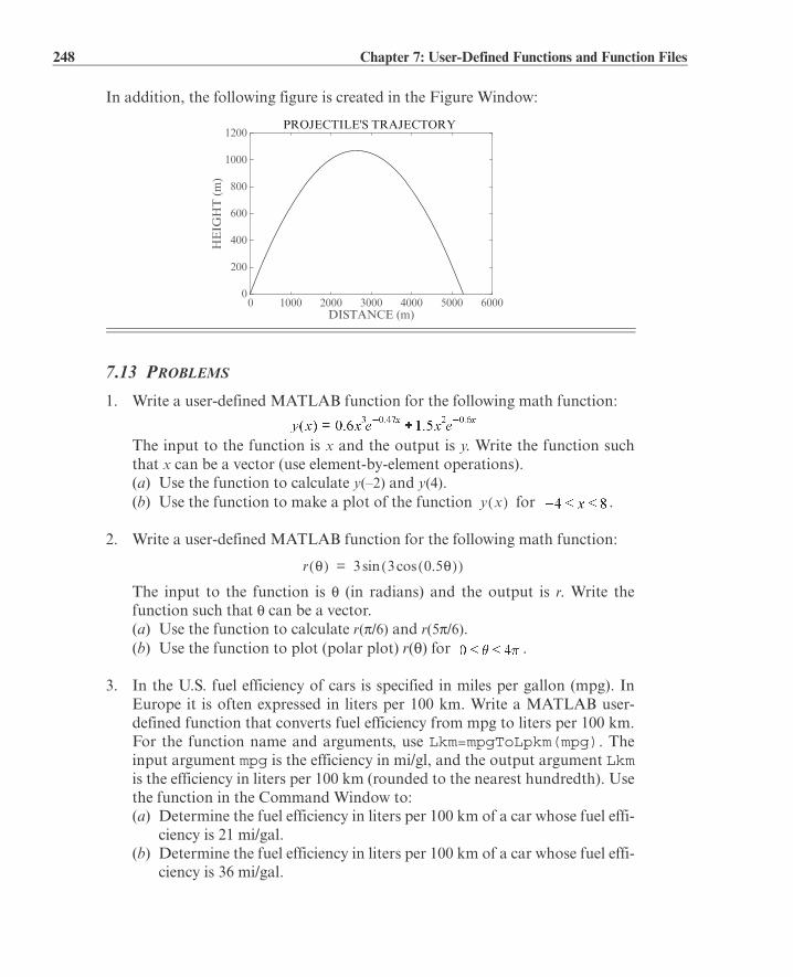
248 Chapter 7: User-Defined Functions and Function Files
In addition, the following figure is created in the Figure Window:
7.13 PROBLEMS
1. Write a user-defined MATLAB function for the following math function:
The input to the function is x and the output is y. Write the function suchthat x can be a vector (use element-by-element operations).(a) Use the function to calculate y(–2) and y(4).(b) Use the function to make a plot of the function for .
2. Write a user-defined MATLAB function for the following math function:
The input to the function is (in radians) and the output is r. Write thefunction such that can be a vector.(a) Use the function to calculate r( /6) and r(5 /6).(b) Use the function to plot (polar plot) r( ) for .
3. In the U.S. fuel efficiency of cars is specified in miles per gallon (mpg). InEurope it is often expressed in liters per 100 km. Write a MATLAB user-defined function that converts fuel efficiency from mpg to liters per 100 km.For the function name and arguments, use Lkm=mpgToLpkm(mpg). Theinput argument mpg is the efficiency in mi/gl, and the output argument Lkmis the efficiency in liters per 100 km (rounded to the nearest hundredth). Usethe function in the Command Window to:(a) Determine the fuel efficiency in liters per 100 km of a car whose fuel effi-
ciency is 21 mi/gal.(b) Determine the fuel efficiency in liters per 100 km of a car whose fuel effi-
ciency is 36 mi/gal.
DISTANCE (m)0 1000 2000 3000 4000 5000 6000
HE
IGH
T (
m)
0
200
400
600
800
1000
1200PROJECTILE'S TRAJECTORY
y x
r 3 3 0.5cossin=

7.13 Problems 249
4. Pressure in U.S. customary units is measured in psi (pound per square inch).
In SI metric units pressure is measured in Pa (N/m2). Write a user-definedMATLAB function that converts pressure given in units of psi to pressure inunits of Pa. For the function name and arguments, use [Pa] = Psi-ToPa(psi). The input argument psi is the pressure in units of psi to beconverted, and the output argument Pa is the converted pressure in units ofPa (rounded to the nearest integer). Use the function in the Command Win-dow to:(a) Convert 120 psi to units of Pa.(b) Convert 3,000 psi to units of Pa.
5. Tables of material properties list density, in units of kg/m3, when the inter-national system of units (SI) is used, and list specific weight, in units of lb/
in.3, when the U.S. customary system of units is used. Write a user-definedMATLAB function that converts density to specific weight. For the func-tion name and arguments, use [sw] = DenToSw(den). The input argu-
ment den is the density of a material in kg/m3, and the output argument sw
is the specific weight in lb/in.3. Use the function in the Command Windowto:
(a) Determine the specific weight of copper whose density is 8,960 kg/m3.
(b) Determine the specific weight of concrete whose density is 2,340 kg/m3.
6. Write a user-defined MATLAB function that converts torque given in unitsof N-m to torque in units of lb-ft. For the function name and arguments,use lbft = NmTOlbft(Nm). The input argument Nm is the torque in N-m,and the output argument lbft is the torque in lb-ft (rounded to the nearestinteger). Use the function to convert 2,000 N-m to units of lb-ft.
7. The body surface area (BSA) in m2 of a person (used for determining dosageof medications) can be calculated by the formula (Mosteller formula):
in which H is the person’s height in inches, and W is the persons weight in lb.Write a MATLAB user-defined function that calculates the body sur-
face area. For the function name and arguments, use BSA = Body-SurA(w,h). The input arguments w and h are the weight and height,respectively. The output argument BSA is the BSA value. Use the function tocalculate the body surface area of:(a) A 170-lb, 5-ft 10-in. tall person.(b) A 220-lb, 6-ft 5-in. tall person.

250 Chapter 7: User-Defined Functions and Function Files
8. The fuel tank shown in the figure in shaped as a halfa sphere with in.
Write a user-defined function that calculates thevolume of fuel in the tank (in gallons) as a functionof the height y (measured from the bottom). For thefunction name and arguments, use V = Vol-fuel(y). Use the function to make a plot of thevolume as a function of y for in.
9. A paper cup is designed to have a geometry of afrustum of a cone. Write a user-defined function thatdetermines the volume and the surface area (side plusbottom) of the cup for given values of r, R, and h. Forthe function name and arguments, use [V, S] =VolSArea(r,R,h). The input arguments r, R, andh are the radius of the base, the radius of the top andthe height, respectively (all in units of inches). The out-put arguments V and S are the volume (in units of U.S.
fluid ounce) and the surface area (in units of in.2),respectively. Use the function to determine the volume and the surface area ofcups with the following dimensions: (a) in., in., in.(b) in., in., in.
10. The relative humidity, RH, at sea level can be calculated from measured val-ues of the dry-bulb temperature, , and the wet-bulb temperature by(temperatures in degrees Celsius):
where VP is the vapor pressure given by:
and SVP is the saturated vapor pressure given by:
Write a user-defined function for calculating RH for given and . Forthe function name and arguments, use RH = RelHum(Tdb,Twb). Theinput arguments are Tdb and Twb are the dry-bulb and wet-buld tempera-tures, respectively in °F. The output argument RH is the relative humidity inpercent (rounded to the nearest integer). Inside the user-defined functionuse a subfunction, or an anonymous function to convert the unit of the tem-perature from Cesius to Fahrenheit. Use the function to determine the rela-tive humidity for the following conditions:(a) F, F. (b) F, F.
y
RR 24=
rh
R
r 2= R 3.5= h 4.25=r 2.5= R 3.5= h 4.5=
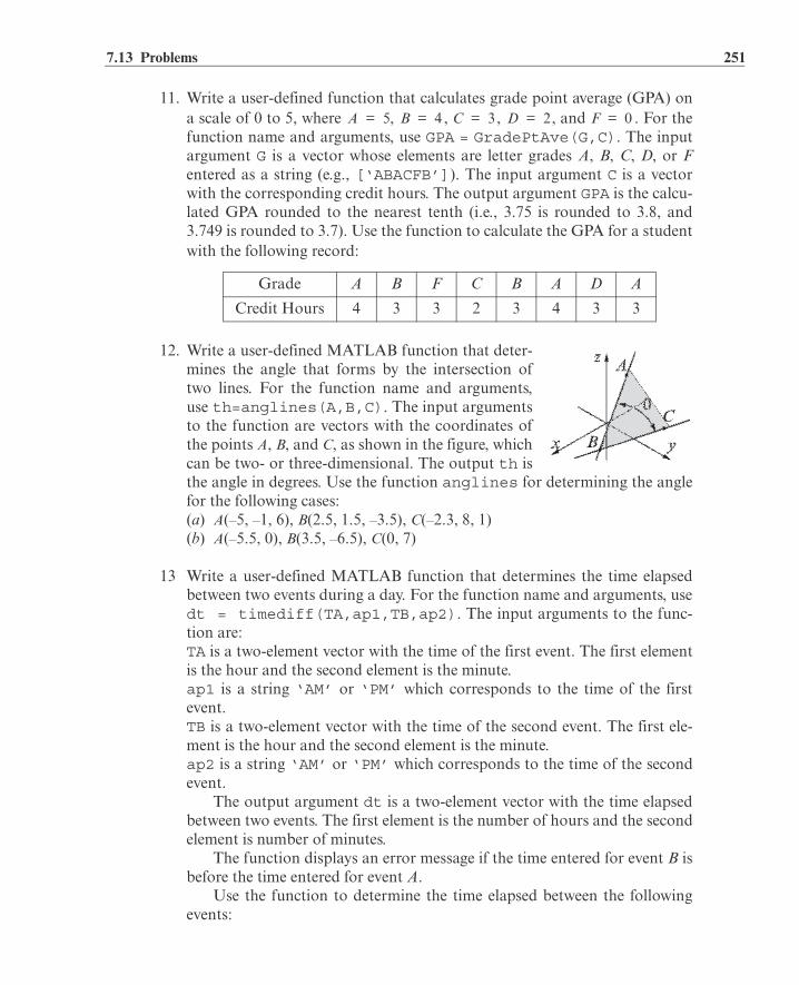
7.13 Problems 251
11. Write a user-defined function that calculates grade point average (GPA) ona scale of 0 to 5, where , , , , and . For thefunction name and arguments, use GPA = GradePtAve(G,C). The inputargument G is a vector whose elements are letter grades A, B, C, D, or Fentered as a string (e.g., [‘ABACFB’]). The input argument C is a vectorwith the corresponding credit hours. The output argument GPA is the calcu-lated GPA rounded to the nearest tenth (i.e., 3.75 is rounded to 3.8, and3.749 is rounded to 3.7). Use the function to calculate the GPA for a studentwith the following record:
12. Write a user-defined MATLAB function that deter-mines the angle that forms by the intersection oftwo lines. For the function name and arguments,use th=anglines(A,B,C). The input argumentsto the function are vectors with the coordinates ofthe points A, B, and C, as shown in the figure, whichcan be two- or three-dimensional. The output th isthe angle in degrees. Use the function anglines for determining the anglefor the following cases:(a) A(–5, –1, 6), B(2.5, 1.5, –3.5), C(–2.3, 8, 1)(b) A(–5.5, 0), B(3.5, –6.5), C(0, 7)
13 Write a user-defined MATLAB function that determines the time elapsedbetween two events during a day. For the function name and arguments, usedt = timediff(TA,ap1,TB,ap2). The input arguments to the func-tion are:TA is a two-element vector with the time of the first event. The first elementis the hour and the second element is the minute.ap1 is a string ‘AM’ or ‘PM’ which corresponds to the time of the firstevent.TB is a two-element vector with the time of the second event. The first ele-ment is the hour and the second element is the minute.ap2 is a string ‘AM’ or ‘PM’ which corresponds to the time of the secondevent.
The output argument dt is a two-element vector with the time elapsedbetween two events. The first element is the number of hours and the secondelement is number of minutes.
The function displays an error message if the time entered for event B isbefore the time entered for event A.
Use the function to determine the time elapsed between the followingevents:
Grade A B F C B A D A
Credit Hours 4 3 3 2 3 4 3 3
A 5= B 4= C 3= D 2= F 0=

252 Chapter 7: User-Defined Functions and Function Files
(a) Event A: 5:37 AM; Event B: 2:51 PM.(b) Event A: 12:53 PM; Event B: 6:12 PM.(c) Event A: 11:32 PM; Event B: 3:18 PM. (Error situation.)
14. Write a user-defined MATLAB function that determines the unit vector inthe direction of the line that connects two points (A and B) in space. For thefunction name and arguments, use n = unitvec(A,B). The input to thefunction are two vectors A and B, each with the Cartesian coordinates of thecorresponding point. The output n is a vector with the components of theunit vector in the direction from A to B. If points A and B have two coordi-nates each (they are in the x y plane), then n is a two-element vector. Ifpoints A and B have three coordinate each (general points in space), then nis a three-element vector. Use the function to determine the following unitvectors:(a) In the direction from point (–0.7, 2.1) to point (9, 18).(b) In the direction from point (10, –3.5, –2.5) to point (–11, 6.5, 5.9).
15. Write a user-defined MATLAB function that determines the cross productof two vectors. For the function name and arguments, use w=cross-pro(u,v). The input arguments to the function are the two vectors, whichcan be two- or three-dimensional. The output w is the result (a vector). Usethe function crosspro for determining the cross product of:(a) Vectors and .(b) Vectors and .
16. The area of a triangle ABC can be calculated by:
where AB is the vector from vertex A to vertex B and AC is the vector fromvertex A to vertex C. Write a user-defined MATLAB function that deter-mines the area of a triangle given its vertices’ coordinates. For the functionname and arguments, use [Area] = TriArea(A,B,C). The input argu-ments A, B, and C are vectors, each with the coordinates of the correspondingvertex. Write the code of TriArea such that it has two subfunctions—onethat determines the vectors AB and AC and another that executes the crossproduct. (If available, use the user-defined functions from Problem 15). Thefunction should work for a triangle in the x-y plane (each vertex is definedby two coordinates) or for a triangle in space (each vertex is defined by threecoordinates). Use the function to determine the areas of triangles with thefollowing vertices:(a) , , (b) , ,
a 3i 11j+=
A 1 2,= B 10 3,= C 6 11,=

7.13 Problems 253
17. As shown in the figure, the area of a convex polygoncan be calculated by adding the area of the trianglesthat the polygon can be divided into. Write a user-defined MATLAB function that calculates the areaof a convex n-sided polygon. For the function nameand arguments, use A = APolygon(Crd). Theinput argument Crd is a two-column matrix whereeach row contains the coordinates of a vertex (first column is the x coordi-nate and the second column is the y coordinate). The vertices are listed inthe order that they are connected to form the polygon (i.e., coordinates ofpoint A in the first row, point B in the second, and so on). The output argu-ment A is the area of the polygon. Write the code of APolygon such that ithas a subfunction that calculates the area of a triangle for given vertices’coordinates. Use APolygon to calculate the area of the polygon shown inthe figure. The coordinates of the vertices are: A(1, 1), B(7, 2), C(10, 5), D(9,11), E(6, 12), F(1, 12), G(–3, 8), H(–4, 4).
18. Write a user-defined function that determines the location of the center andthe radius of a circle that passes through three given points in a plane. Thefunction also creates a plot that shows the circle and the points. For thefunction name and arguments, use [C R]=Circle3Pts(A,B,C). Theinput arguments A, B, and C are each a two-element vector with the x and ycoordinates of the corresponding point. The output argument C, is a vectorwith the coordinates of the center the output argument R, is the radius (bothrounded to the nearest hundredth). Use the function with the followingthree points: A(7, 1.2), B(0.5, 2.6), and C(–2.4, –1.4).
19. Write a user-defined MATLAB function that converts integers written indecimal form to binary form. Name the function b=Bina(d), where theinput argument d is the integer to be converted and the output argument bis a vector with 1s and 0s that represents the number in binary form. Thelargest number that could be converted with the function should be a binarynumber with 16 1s. If a larger number is entered as d, the function shoulddisplay an error message. Use the function to convert the following num-bers:(a) 100 (b) 1,002 (c) 52,601 (d) 200,090
20. Write a user-defined function that plots a triangle and the circle that isinscribed inside, given the coordinates of its vertices. For the function nameand arguments, use TriCirc(A,B,C). The input arguments are vectorswith the x and y coordinates of the vertices, respectively. This function hasno output arguments. Use the function with the points (2.6, 3.2), (11, 14.5),and (–2, 2.8).
AB
C
DEF
G
H

254 Chapter 7: User-Defined Functions and Function Files
21. Write a user-defined function that plots anellipse with axes that are parallel to the x and yaxes, given the coordinates of its vertices andthe coordinates of another point that the ellipsepasses through. For the function name andarguments, use ellipseplot(A,B,C). Theinput arguments A and B are each a two-elementvector with the coordinates of the vertices, and C is a two-element vectorwith the coordinates of another point on the ellipse (see figure), respectively.This function has no output arguments. Use the function to plot the follow-ing ellipses:(a) A(2,3), B(11,3), C(10,4) (b) A(2,11), B(2,–4), C(4,8)
22. In polar coordinates a two-dimensional vectoris given by its radius and angle . Write auser-defined MATLAB function that adds twovectors that are given in polar coordinates. Forthe function name and arguments, use[r th]= AddVecPol(r1,th1,r2,th2),
where the input arguments are and, and the output arguments are the
radius and angle of the result. Use the function to carry out the followingadditions: (a) , (b) ,
23. Write a user-defined function that determines if a number is a prime num-ber. Name the function pr=Trueprime(m), where the input arguments mis a positive integer and the output argument pr is 1 if m is a prime numberand 0 if m is not a prime number. Do not use MATLAB’s built-in functionsprimes and isprime. If a negative number or a number that is not aninteger is entered when the function is called, the error message “The inputargument must be a positive integer.” is displayed. (a) Use the function with 733, 2001, and 107.5.(b) Write a MATLAB program in a script file that makes use of Truep-rime and finds the smallest prime number that remains a prime numberwhen added to its reverse (37 is the reverse of 73).
24. The harmonic mean H of a set of n positivenumbers is defined by:
Write a user-defined function that calculatesthe harmonic mean of a set of numbers. Forfunction name and arguments use G=Harmean(x), where the input argu-
x
y
A BC
r,
r1 1,r2 2,
r1 5 23,= r2 12 40,= r1 6 80,= r2 15 125,=
x1 x2 xn, , ,

7.13 Problems 255
ment x is a vector of numbers (any length) and the output argument H istheir harmonic mean. In electrical engineering the equivalent resistance ofresistors connected in parallel is equal to the harmonic mean of the valuesof the resistors divided by the number of the resistors. Use the user-definedfunction Harmean to calculate the equivalent resistance of the resistorsshown in the figure.
25. Write a user-defined function that determines the polarcoordinates of a point from the Cartesian coordinates ina two-dimensional plane. For the function name andarguments, use [th rad]=CartToPolar(x,y).The input arguments are the x and y coordinates of thepoint, and the output arguments are the angle and theradial distance to the point. The angle is in degrees andis measured relative to the positive x axis, such that it is a positive number inquadrants I and II, and a negative number in quadrant III and IV. Use the func-tion to determine the polar coordinates of points (14, 9), (–11, –20), (–15, 4),and (13.5, –23.5).
26. Write a user-defined function that determines the value that occurs mostoften in a set of data that is given in a two-dimensional matrix. For the func-tion name and arguments, use [v, q] =matrixmode(x). The input argu-ment x is a matrix of any size with numerical values, and the outputarguments v and q are the values that occur most often and the number oftimes they occur. If there are two, or more, values that occur most oftenthan v is a vector with these values. Do not use the MATLAB built-in func-tion mode. Test the function three times. For input create a matrixusing the following command: x=randi(10,5,6).
27. Write a user-defined function that sorts the elements of a vector from the
largest to the smallest. For the function name and arguments, usey=downsort(x). The input to the function is a vector x of any length,and the output y is a vector in which the elements of x are arranged in adescending order. Do not use the MATLAB built-in functions sort, max,or min. Test your function on a vector with 14 numbers (integers) randomlydistributed between –30 and 30. Use the MATLAB randi function togenerate the initial vector.
28. Write a user-defined function that sorts the elements of a matrix. For thefunction name and arguments, use B = matrixsort(A), where A is anysize matrix and B is a matrix of the same size with the elements of Arearranged in descending order column after column with the (1,1) elementthe largest and the (m,n) element the smallest. If available, use the user-defined function downsort from the previous problem as a subfunction

256 Chapter 7: User-Defined Functions and Function Files
within matrixsort.Test your function on a matrix with elements (integers) randomly
distributed between –30 and 30. Use MATLAB’s randi function to gener-ate the initial matrix.
29. Write a user-defined MATLAB function that finds the largest element of amatrix. For the function name and arguments, use [Em,rc] = matrix-max(A), where A is any size matrix. The output argument Em is the value ofthe largest element, and rc is a two-element vector with the address of thelargest element (row and column numbers). If there are two, or more, ele-ments that have the maximum value, the output argument rc is a two-col-umn matrix where the rows list the addresses of the elements. Test thefunction three times. For input create a matrix using the followingcommand: x=randi([-20 100],4,6).
30. Write a user-defined MATLAB function that calculates the determinant ofa matrix by using the formula:
For the function name and arguments, use d3 = det3by3(A), where theinput argument A is the matrix and the output argument d3 is the value ofthe determinant. Write the code of det3by3 such that it has a subfunctionthat calculates the determinant. Use det3by3 for calculating thedeterminants of:
(a) (b)
31. The shortest distance between two points on the surface of the globe (great-circle distance) can be calculated by using the haversine formula. If and
are the latitude and longitude of point 1 and and are the latitudeand longitude of point 2, the great circle distance between the points is givenby:
where , and mi is
the Earth radius. Write a user-defined function that determines the distancebetween two points on the Earth. For the function name and arguments, usedis = GreatCirDis(Lat1,Lng1,Lat2,Lng2), where the input argu-ments are the latitude and longitude of the two points (degrees in decimalformat), and dis is the great-circle distance in miles. Use the function tocalculate the distance between London (51.50853°, –0.12574°) and New

7.13 Problems 257
York City (40.71427°, –74.00597°).32. Delta rosette is a set of three strain gages oriented at
120° relative to each other. The strain measuredwith each of the strain gages is , , and . Theprincipal strains and can be calculated fromthe strains measured with the rosette by:
Write a user-defined MATLAB function that deter-mines the principal strains given the strains , ,and . For the function name and arguments, use[P1, P2]=DeltaRos(A,B,C). The input arguments A, B, and C are thevalues of the three strains measured by the rosette. The output argumentsP1 and P2 are the values of the principal strains.
Use the function to determine the principal strains for the followingcases:(a) , , .(b) , , .
33. In a lottery the player has to select several numbers out of a list. Write auser-defined function that generates a list of n integers that are uniformlydistributed between the numbers a and b. All the selected numbers on the listmust be different. For function name and arguments, usex=lotto(a,b,n)where the input arguments are the numbers a and b, andn, respectively. The output argument x is a vector with the selected numbers. (a) Use the function to generate a list of seven numbers from the numbers 1
through 59.(b) Use the function to generate a list of eight numbers from the numbers
50 through 65.(c) Use the function to generate a list of nine numbers from the numbers
–25 through –2.
34. The Taylor series expansion for about is given by:
where x is in radians. Write a user-defined function that determines using Taylor’s series expansion. For function name and arguments, usey=sinTay(x), where the input argument x is the angle in degrees and theoutput argument y is the value of . Inside the user-defined function,use a loop for adding the terms of the Taylor series. If is the nth term inthe series, then the sum of the n terms is . In each pass, cal-
culate the estimated error E given by . Stop adding terms when
A B C
1 2
A B
C
xsin x 0=
n 0=
xsin
xsinan
Sn

258 Chapter 7: User-Defined Functions and Function Files
. Since (n is an integer) write the user-defined function such that if the angle is larger than 360°, or smaller than–360°, then the Taylor series will be calculated using the smallest number ofterms (using a value for x that is closest to 0).
Use sinTay for calculating:(a) (b) (c) .(d) (e) (f)
Compare the values calculated using sinTay with the values obtainedby using MATLAB’s built-in sind function.
35. Write a user-defined function that determinesthe coordinate of the centroid of the I-shaped cross-sectional area shown in the figure.For the function name and arguments, use yc =centroidI(w,h,d,t), where the inputarguments w, h, d, and t are the dimensionsshown in the figure and the output argumentyc is the coordinate .
Use the function to determine for a beam with in., in.,in., and in.
36. The area moment of inertia of a rectangle about the
axis passing through its centroid is . The
moment of inertia about an axis x that is parallel to is
given by , where A is the area of the rect-
angle, and is the distance between the two axes.
Write a MATLAB user-defined function thatdetermines the area moment of inertia of a I-beam about the axis that passes through its cen-troid (see drawing). For the function name andarguments use Ixc=IxcBeam(w,h,d,t),where the input arguments w, h, d, and t are thedimensions shown in the figure and the outputargument Ixc is . For finding the coordinate
of the centroid, use the user-defined function centroidI from the pre-vious problem as a subfunction inside IxcBeam. (The moment of inertia of a composite area is obtained by dividing the areainto parts and adding the moments of inertia of the parts.)
Use the function to determine the moment of inertia for a beam within., in., in., and in.
39sin 205sin754sin
w
h
t
d
yc
c
t
t
yc
yc
yc w 10= h 8=d 6= t 0.5=
b
h
dx
xo
x
Ixo
xo
xo
Ix IxoAd x
2+=
dx
w
h
t
d
yc
c
t
t
Ixc
Ixc
yc
w 10= h 8= d 6= t 0.5=

7.13 Problems 259
37. The simple RC high-pass filter shown in thefigure passes signals with frequencies higherthan a certain cutoff frequency. The ratio ofthe magnitudes of the voltages is given by:
where , and f is the frequency of the input signal.Write a user-defined MATLAB function that calculates the ratio of
magnitudes for given values of R, C, and f. For the function name and argu-ments, use RV = RCFilt(R,C,f). The input arguments are R, the size ofthe resistor in (ohms); C, the size of the capacitor in F (farad); and f, thefrequency of the input signal in Hz (hertz). Write the function such that fcan be a vector.
Write a program in a script file that uses the RCFilt function to gener-ate a plot of RV as a function of f for Hz. The plot has alogarithmic scale on the horizontal axis. When executed, the script file asksthe user to enter the values of R and C. Label the axes of the plot.
Run the script file with , and F.
38. A circuit that filters out a certain fre-quency is shown in the figure. In this fil-ter, the ratio of the magnitudes of thevoltages is given by:
where , and f is the frequency of the input signal.Write a user-defined MATLAB function that calculates the ratio of
magnitudes. For the function name and arguments, use RV=filt-afreq(R,C,L,f). The input arguments are R the size of the resistor in (ohms); C, the size of the capacitor in F (farad); L, the inductance of the coilin H (henrys); and f, the frequency of the input signal in Hz (hertz). Writethe function such that f can be a vector.
Write a program in a script file that uses the filtafreq function togenerate a figure with two plots of RV as a function of f for Hz. In one plot F, mH, and , and in the sec-ond plot C and L are unchanged but .. The plot has a logarithmicscale on the horizontal axis. Label the axes and display a legend.
39. The first derivative of a function at a point can be
approximated with the four-point central difference formula:
R 80=
Vi Vo
C
L
R
C 160= L 45= R 200=R 50=
f x x x0=
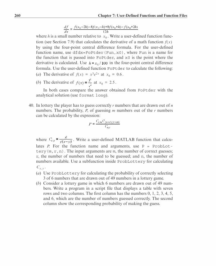
260 Chapter 7: User-Defined Functions and Function Files
where h is a small number relative to . Write a user-defined function func-tion (see Section 7.9) that calculates the derivative of a math function by using the four-point central difference formula. For the user-definedfunction name, use dfdx=FoPtder(Fun,x0), where Fun is a name forthe function that is passed into FoPtder, and x0 is the point where thederivative is calculated. Use in the four-point central differenceformula. Use the user-defined function FoPtder to calculate the following:(a) The derivative of at .
(b) The derivative of at .
In both cases compare the answer obtained from FoPtder with theanalytical solution (use format long).
40. In lottery the player has to guess correctly r numbers that are drawn out of nnumbers. The probability, P, of guessing m numbers out of the r numberscan be calculated by the expression:
where . Write a user-defined MATLAB function that calcu-
lates P. For the function name and arguments, use P = ProbLot-tery(m,r,n). The input arguments are m, the number of correct guesses;r, the number of numbers that need to be guessed; and n, the number ofnumbers available. Use a subfunction inside ProbLottery for calculating
.
(a) Use ProbLottery for calculating the probability of correctly selecting3 of 6 numbers that are drawn out of 49 numbers in a lottery game.
(b) Consider a lottery game in which 6 numbers are drawn out of 49 num-bers. Write a program in a script file that displays a table with sevenrows and two columns. The first column has the numbers 0, 1, 2, 3, 4, 5,and 6, which are the number of numbers guessed correctly. The secondcolumn show the corresponding probability of making the guess.
x0
f x
f x x3e2x= x0 0.6=
x0 2.5=
Cx y,
261
Chapter 8 Polynomials, Curve Fitting, and Interpolation
Polynomials are mathematical expressions that are frequently used for problemsolving and modeling in science and engineering. In many cases an equationthat is written in the process of solving a problem is a polynomial, and the solu-tion of the problem is the zero of the polynomial. MATLAB has a wide selec-tion of functions that are specifically designed for handling polynomials. Howto use polynomials in MATLAB is described in Section 8.1.
Curve fitting is a process of finding a function that can be used to modeldata. The function does not necessarily pass through any of the points, butmodels the data with the smallest possible error. There are no limitations to thetype of the equations that can be used for curve fitting. Often, however, polyno-mial, exponential, and power functions are used. In MATLAB curve fitting canbe done by writing a program or by interactively analyzing data that is displayedin the Figure Window. Section 8.2 describes how to use MATLAB program-ming for curve fitting with polynomials and other functions. Section 8.4describes the basic fitting interface that is used for interactive curve fitting andinterpolation.
Interpolation is the process of estimating values between data points. Thesimplest kind of interpolation is done by drawing a straight line between thepoints. In a more sophisticated interpolation, data from additional points isused. How to interpolate with MATLAB is discussed in Sections 8.3 and 8.4.
8.1 POLYNOMIALS
Polynomials are functions that have the form:
The coefficients are real numbers, and n which is a nonnegative

262 Chapter 8: Polynomials, Curve Fitting, and Interpolation
integer, is the degree, or order, of the polynomial.Examples of polynomials are:
polynomial of degree 5.
polynomial of degree 2. polynomial of degree 1.
A constant (e.g., ) is a polynomial of degree 0.In MATLAB, polynomials are represented by a row vector in which the ele-
ments are the coefficients . The first element is the coefficient ofthe x with the highest power. The vector has to include all the coefficients,including the ones that are equal to 0. For example:
8.1.1 Value of a Polynomial
The value of a polynomial at a point x can be calculated with the functionpolyval that has the form:
x can also be a vector or a matrix. In such a case the polynomial is calculatedfor each element (element-by-element), and the answer is a vector, or a matrix,with the corresponding values of the polynomial.
Sample Problem 8-1: Calculating polynomials with MATLAB
For the polynomial :(a) Calculate .(b) Plot the polynomial for .
Solution
The problem is solved in the Command Window.(a) The coefficients of the polynomials are assigned to vector p. The function
Polynomial MATLAB representation
p = [8 5]
d = [2 –4 10]
, MATLAB form: h = [6 0 –150]
, MATLAB form:
c = [5 0 0 6 7 0]
f x 5x5 6x2 7x 3+ + +=
f x 6=
8x 5+
polyval(p,x)
p is a vector with the coef-ficients of the polynomial.
x is a number, or a variable that has an assigned value, or a com-putable expression.
f 9

8.1 Polynomials 263
polyval is then used to calculate the value at x = 9.
(b) To plot the polynomial, a vector x is first defined with elements rangingfrom –1.5 to 6.7. Then a vector y is created with the values of the polynomial forevery element of x. Finally, a plot of y vs. x is made.
The plot created by MATLAB is presented below (axis labels were added withthe Plot Editor).
8.1.2 Roots of a Polynomial
The roots of a polynomial are the values of the argument for which the value ofthe polynomial is equal to zero. For example, the roots of the polynomial
are the values of x for which , which are and x = 3.
MATLAB has a function, called roots, that determines the root, or roots,of a polynomial. The form of the function is:
For example, the roots of the polynomial in Sample Problem 8-1 can be deter-mined by:
>> p = [1 -12.1 40.59 -17.015 -71.95 35.88];
>> polyval(p,9)
ans = 7.2611e+003
>> x=-1.5:0.1:6.7;
>> y=polyval(p,x);
>> plot(x,y)
Calculating the value of the polyno-mial for each element of the vector x.
x-2 -1 0 1 2 3 4 5 6 7
y
-200
-150
-100
-50
0
50
100
150
r = roots(p)
p is a row vector with the coef-ficients of the polynomial.
r is a column vector withthe roots of the polynomial.

264 Chapter 8: Polynomials, Curve Fitting, and Interpolation
The roots command is very useful for finding the roots of a quadratic equa-
tion. For example, to find the roots of , type:
When the roots of a polynomial are known, the poly command can beused for determining the coefficients of the polynomial. The form of the polycommand is:
For example, the coefficients of the polynomial in Sample Problem 8-1 can beobtained from the roots of the polynomial (see above) by:
8.1.3 Addition, Multiplication, and Division of Polynomials
Addition:
Two polynomials can be added (or subtracted) by adding (subtracting) the vec-tors of the coefficients. If the polynomials are not of the same order (whichmeans that the vectors of the coefficients are not of the same length), the shortervector has to be modified to be of the same length as the longer vector by add-ing zeros (called padding) in front. For example, the polynomials
and can be addedby:
>> p= 1 -12.1 40.59 -17.015 -71.95 35.88];
>> r=roots(p)
r = 6.5000 4.0000 2.3000 -1.2000 0.5000
>> roots([4 10 -8])
ans = -3.1375 0.6375
>> r=[6.5 4 2.3 -1.2 0.5];
>> p=poly(r)
p = 1.0000 -12.1000 40.5900 -17.0150 -71.9500 35.8800
When the roots are known, the polynomial canactually be written as:
p = poly(r)
r is a vector (row or column) with the roots of the polynomial.
p is a row vector with the coef-ficients of the polynomial.

8.1 Polynomials 265
Multiplication:
Two polynomials can be multiplied using the MATLAB built-in function conv,which has the form:
• The two polynomials do not have to be of the same order.
• Multiplication of three or more polynomials is done by using the conv functionrepeatedly.
For example, multiplication of the polynomials and above gives:
which means that the answer is:
Division:
A polynomial can be divided by another polynomial with the MATLAB built-infunction deconv, which has the form:
For example, dividing by is done by:
>> p1=[3 15 0 -10 -3 15 -40];
>> p2=[3 0 -2 -6];
>> p=p1+[0 0 0 p2]
p = 3 15 0 -7 -3 13 -46
>> pm=conv(p1,p2)
pm = 9 45 -6 -78 -99 65 -54 -12 -10 240
>> u=[2 9 7 -6];
>> v=[1 3];
Three 0s are added in front of p2, since the order of p1 is 6 and the order of p2 is 3.
c = conv(a,b)
a and b are the vectors of thecoefficients of the polynomialsthat are being multiplied.
c is a vector of the coefficients of the polynomial that is the product of the multiplication.
f1 x f2 x
[q,r] = deconv(u,v)
u is a vector with the coefficients ofthe numerator polynomial.v is a vector with the coefficients ofthe denominator polynomial.
q is a vector with the coefficientsof the quotient polynomial.r is a vector with the coefficientsof the remainder polynomial.
x 3+

266 Chapter 8: Polynomials, Curve Fitting, and Interpolation
An example of division that gives a remainder is
divided by :
The answer is: .
8.1.4 Derivatives of Polynomials
The built-in function polyder can be used to calculate the derivative of a sin-gle polynomial, a product of two polynomials, or a quotient of two polynomials,as shown in the following three commands.
k = polyder(p) Derivative of a single polynomial. p is a vector withthe coefficients of the polynomial. k is a vector withthe coefficients of the polynomial that is the deriva-tive.
k = polyder(a,b) Derivative of a product of two polynomials. a and bare vectors with the coefficients of the polynomialsthat are multiplied. k is a vector with the coefficientsof the polynomial that is the derivative of the product.
[n d]= polyder(u,v) Derivative of a quotient of two polynomials. u and vare vectors with the coefficients of the numerator anddenominator polynomials. n and d are vectors withthe coefficients of the numerator and denominatorpolynomials in the quotient that is the derivative.
The only difference between the last two commands is the number of outputarguments. With two output arguments MATLAB calculates the derivative ofthe quotient of two polynomials. With one output argument, the derivative is ofthe product.
>> [a b]=deconv(u,v)
a = 2 3 -2
b = 0 0 0 0
>> w=[2 -13 0 75 2 0 -60];
>> z=[1 0 -5];
>> [g h]=deconv(w,z)
g = 2 -13 10 10 52
h = 0 0 0 0 0 50 200
The answer is: .
Remainder is zero.
The quotient is: .
The remainder is: .

8.2 Curve Fitting 267
For example, if , and , the derivatives of
, , and can be determined by:
8.2 CURVE FITTING
Curve fitting, also called regression analysis, is a process of fitting a function toa set of data points. The function can then be used as a mathematical model ofthe data. Since there are many types of functions (linear, polynomial, power,exponential, etc.), curve fitting can be a complicated process. Many times onehas some idea of the type of function that might fit the given data and will needonly to determine the coefficients of the function. In other situations, wherenothing is known about the data, it is possible to make different types of plotsthat provide information about possible forms of functions that might fit thedata well. This section describes some of the basic techniques for curve fittingand the tools that MATLAB has for this purpose.
8.2.1 Curve Fitting with Polynomials; The polyfit Function
Polynomials can be used to fit data points in two ways. In one the polynomialpasses through all the data points, and in the other the polynomial does not nec-essarily pass through any of the points but overall gives a good approximationof the data. The two options are described below.
Polynomials that pass through all the points:
When n points (xi, yi) are given, it is possible to write a polynomial of degree that passes through all the points. For example, if two points are given it
is possible to write a linear equation in the form of that passesthrough the points. With three points, the equation has the form of
>> f1= 3 -2 4];>> f2=[1 0 5];
>> k=polyder(f1)
k = 6 -2
>> d=polyder(f1,f2)
d = 12 -6 38 -10
>> [n d]=polyder(f1,f2)
n = 2 22 -10
d = 1 0 10 0 25
Creating the vectors of coefficients of f1 and f2.
The derivative of f1 is: .
The derivative of f1*f2 is: .
The derivative of is: .
y mx b+=

268 Chapter 8: Polynomials, Curve Fitting, and Interpolation
. With n points the polynomial has the form
. The coefficients of the polynomial are deter-mined by substituting each point in the polynomial and then solving the n equa-tions for the coefficients. As will be shown later in this section, polynomials ofhigh degree might give a large error if they are used to estimate values betweendata points.
Polynomials that do not necessarily pass through any of the points:
When n points are given, it is possible to write a polynomial of degree less than that does not necessarily pass through any of the points but that overall
approximates the data. The most common method of finding the best fit to datapoints is the method of least squares. In this method, the coefficients of thepolynomial are determined by minimizing the sum of the squares of the residu-als at all the data points. The residual at each point is defined as the differencebetween the value of the polynomial and the value of the data. For example,consider the case of finding the equation of a straight line that best fits four datapoints as shown in Figure 8-1. The points are , , , and
, and the polynomial of the first degree can be written as. The residual, , at each point is the difference between the
value of the function at and , . An equation for the sum ofthe squares of the residuals of all the points is given by:
or, after substituting the equation of the polynomial at each point, by:
At this stage R is a function of and . The minimum of R can be determinedby taking the partial derivative of R with respect to and (two equations)and equating them to zero:
and
Figure 8-1: Least squares fitting of first-degree polynomial to four points.
x1 y1, x2 y2, x3 y3,
R2
R1
R3
x
y
R4
f(x1)f(x2)
f(x3)
f(x4)
(x2, y2) f(x) = a1x + a0
(x4, y4)
(x3, y3)
(x1, y1)
x4 y4,f x a1x a0+= Ri
xi yi
Ri
a1 a0
a1 a0

8.2 Curve Fitting 269
This results in a system of two equations with two unknowns, and . Thesolution of these equations gives the values of the coefficients of the polynomialthat best fits the data. The same procedure can be followed with more pointsand higher-order polynomials. More details on the least squares method can befound in books on numerical analysis.
Curve fitting with polynomials is done in MATLAB with the polyfitfunction, which uses the least squares method. The basic form of the polyfitfunction is:
For the same set of m points, the polyfit function can be used to fit poly-nomials of any order up to . If n = 1 the polynomial is a straight line, if n= 2 the polynomial is a parabola, and so on. The polynomial passes through allthe points if (the order of the polynomial is one less than the numberof points). It should be pointed out here that a polynomial that passes throughall the points, or polynomials with higher order, do not necessarily give a betterfit overall. High-order polynomials can deviate significantly between the datapoints.
Figure 8-2 shows how polynomials of different degrees fit the same set ofdata points. A set of seven points is given by (0.9, 0.9), (1.5, 1.5), (3, 2.5), (4, 5.1),
Figure 8-2: Fitting data with polynomials of different order.
a1 a0
p = polyfit(x,y,n)
x is a vector with the horizontal coordinates of the data points (independent variable).y is a vector with the vertical coordinates ofthe data points (dependent variable).n is the degree of the polynomial.
p is the vector of the coeffi-cients of the polynomial that fits the data.
x0 2 4 6 8 10
y
0
1
2
3
4
5
6
7
n=1
0 2 4 6 8 10
y
0
1
2
3
4
5
6
7
n=2

270 Chapter 8: Polynomials, Curve Fitting, and Interpolation
(6, 4.5), (8, 4.9), and (9.5, 6.3). The points are fitted using the polyfit func-tion with polynomials of degrees 1 through 6. Each plot in Figure 8-2 shows thesame data points, marked with circles, and a curve-fitted line that correspondsto a polynomial of the specified degree. It can be seen that the polynomial with n= 1 is a straight line, and that with n = 2 is a slightly curved line. As the degree ofthe polynomial increases, the line develops more bends such that it passes closerto more points. When n = 6, which is one less than the number of points, the linepasses through all the points. However, between some of the points, the linedeviates significantly from the trend of the data.
The script file used to generate one of the plots in Figure 8-2 (the polyno-mial with n = 3) is shown below. Note that in order to plot the polynomial (theline), a new vector xp with small spacing is created. This vector is then used
x=[0.9 1.5 3 4 6 8 9.5];
y=[0.9 1.5 2.5 5.1 4.5 4.9 6.3];
p=polyfit(x,y,3)
xp=0.9:0.1:9.5;
yp=polyval(p,xp);
plot(x,y,'o',xp,yp)
xlabel('x'); ylabel('y')
Figure 8-2: Fitting data with polynomials of different order. (Continued)
x0 2 4 6 8 10
y
0
1
2
3
4
5
6
7
n=3 n = 4
x0 2 4 6 8 10
y
0
1
2
3
4
5
6
7
n=4
x0 2 4 6 8 10
y
0
1
2
3
4
5
6
7
n=5
x0 2 4 6 8 10
y
0
2
4
6
8
10
n=6
Create vectors x and y with thecoordinates of the data points.
Create a vector p using the polyfit function.
Create a vector xp to be used for plotting the polynomial.
Create a vector yp with values of the polynomial at each xp.
A plot of the seven points and the polynomial.

8.2 Curve Fitting 271
with the function polyval to create a vector yp with the value of the polyno-mial for each element of xp.
When the script file is executed, the following vector p is displayed in theCommand Window.
This means that the polynomial of the third degree in Figure 8-2 has the form
.
8.2.2 Curve Fitting with Functions Other than Polynomials
Many situations in science and engineering require fitting functions that are notpolynomials to given data. Theoretically, any function can be used to modeldata within some range. For a particular data set, however, some functions pro-vide a better fit than others. In addition, determining the best-fitting coefficientscan be more difficult for some functions than for others. This section coverscurve fitting with power, exponential, logarithmic, and reciprocal functions,which are commonly used. The forms of these functions are:
(power function)
or (exponential function) or (logarithmic function)
(reciprocal function)
All of these functions can easily be fitted to given data with the polyfit func-tion. This is done by rewriting the functions in a form that can be fitted with alinear polynomial (n = 1), which is
The logarithmic function is already in this form, and the power, exponential,and reciprocal equations can be rewritten as:
(power function) or (exponential function)
(reciprocal function)
These equations describe a linear relationship between and for thepower function, between and x for the exponential function, between yand or for the logarithmic function, and between 1/y and x for thereciprocal function. This means that the polyfit(x,y,1) function can beused to determine the best-fit constants m and b for best fit if, instead of x and y,
p = 0.0220 -0.4005 2.6138 -1.4158
y bxm=
y bemx= y b10mx=
y m xln b+= y m xlog b+=
y mx b+=
yln m xln bln+=
yln mx bln+= ylog mx blog+=
yln xlnyln
xln xlog

272 Chapter 8: Polynomials, Curve Fitting, and Interpolation
the following arguments are used.
The result of the polyfit function is assigned to p, which is a two-elementvector. The first element, p(1), is the constant m, and the second element,p(2), is b for the logarithmic and reciprocal functions, or for the
exponential function, and for the power function ( or
for the exponential function, and for the power func-tion).
For given data it is possible to estimate, to some extent, which of the func-tions has the potential for providing a good fit. This is done by plotting the datausing different combinations of linear and logarithmic axes. If the data points inone of the plots appear to fit a straight line, the corresponding function can pro-vide a good fit according to the list below.
Other considerations in choosing a function:
• Exponential functions cannot pass through the origin.
• Exponential functions can fit only data with all positive y’s or all negative y’s.
• Logarithmic functions cannot model x = 0 or negative values of x.
• For the power function y = 0 when x = 0.
• The reciprocal equation cannot model y = 0.
Function polyfit function form
power p=polyfit(log(x),log(y),1)
exponential or
p=polyfit(x,log(y),1) orp=polyfit(x,log10(y),1)
logarithmic or
p=polyfit(log(x),y,1) orp=polyfit(log10(x),y,1)
reciprocal p=polyfit(x,1./y,1)
x axis y axis Function
linear linear linear
logarithmic logarithmic power
linear logarithmic exponential or
logarithmic linear logarithmic or
linear linear(plot 1/y)
reciprocal
y bxm=
y bemx=
y b10mx=
y m xln b+=y m xlog b+=
bln blog
bln b e p 2=
b 10 p 2= b e p 2=
y mx b+=
y bxm=
y bemx= y b10mx=
y m xln b+= y m xlog b+=
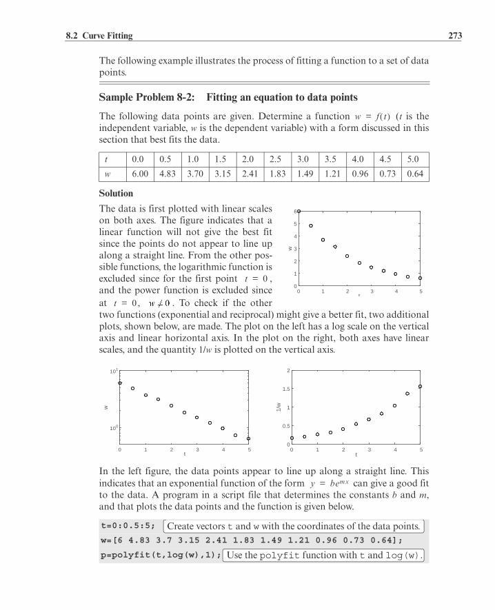
8.2 Curve Fitting 273
The following example illustrates the process of fitting a function to a set of datapoints.
Sample Problem 8-2: Fitting an equation to data points
The following data points are given. Determine a function (t is theindependent variable, w is the dependent variable) with a form discussed in thissection that best fits the data.
Solution
The data is first plotted with linear scaleson both axes. The figure indicates that alinear function will not give the best fitsince the points do not appear to line upalong a straight line. From the other pos-sible functions, the logarithmic function isexcluded since for the first point ,and the power function is excluded sinceat , . To check if the othertwo functions (exponential and reciprocal) might give a better fit, two additionalplots, shown below, are made. The plot on the left has a log scale on the verticalaxis and linear horizontal axis. In the plot on the right, both axes have linearscales, and the quantity 1/w is plotted on the vertical axis.
In the left figure, the data points appear to line up along a straight line. Thisindicates that an exponential function of the form can give a good fitto the data. A program in a script file that determines the constants b and m,and that plots the data points and the function is given below.
t 0.0 0.5 1.0 1.5 2.0 2.5 3.0 3.5 4.0 4.5 5.0
w 6.00 4.83 3.70 3.15 2.41 1.83 1.49 1.21 0.96 0.73 0.64
t=0:0.5:5;
w=[6 4.83 3.7 3.15 2.41 1.83 1.49 1.21 0.96 0.73 0.64];
p=polyfit(t,log(w),1);
w f t=
t0 1 2 3 4 5
w0
1
2
3
4
5
6
t 0=
t 0=
t0 1 2 3 4 5
w
100
101
t0 1 2 3 4 5
1/w
0
0.5
1
1.5
2
y bemx=
Create vectors t and w with the coordinates of the data points.
Use the polyfit function with t and log(w).
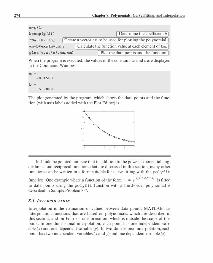
274 Chapter 8: Polynomials, Curve Fitting, and Interpolation
When the program is executed, the values of the constants m and b are displayedin the Command Window.
The plot generated by the program, which shows the data points and the func-tion (with axis labels added with the Plot Editor) is
It should be pointed out here that in addition to the power, exponential, log-arithmic, and reciprocal functions that are discussed in this section, many otherfunctions can be written in a form suitable for curve fitting with the polyfit
function. One example where a function of the form is fittedto data points using the polyfit function with a third-order polynomial isdescribed in Sample Problem 8-7.
8.3 INTERPOLATION
Interpolation is the estimation of values between data points. MATLAB hasinterpolation functions that are based on polynomials, which are described inthis section, and on Fourier transformation, which is outside the scope of thisbook. In one-dimensional interpolation, each point has one independent vari-able (x) and one dependent variable (y). In two-dimensional interpolation, eachpoint has two independent variables (x and y) and one dependent variable (z).
m=p(1)
b=exp(p(2))
tm=0:0.1:5;
wm=b*exp(m*tm);
plot(t,w,'o',tm,wm)
m = -0.4580
b = 5.9889
Determine the coefficient b.
Create a vector tm to be used for plotting the polynomial.
Calculate the function value at each element of tm.
Plot the data points and the function.
t0 1 2 3 4 5
w
0
1
2
3
4
5
6
y ea2x2 a1x a0+ +
=
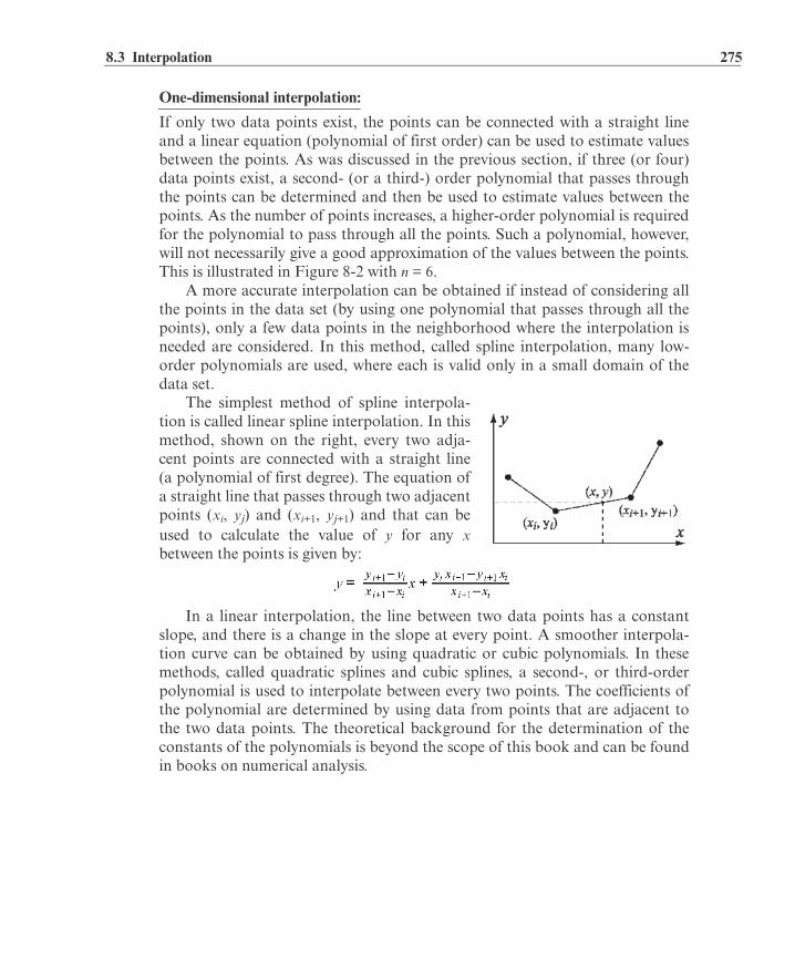
8.3 Interpolation 275
One-dimensional interpolation:
If only two data points exist, the points can be connected with a straight lineand a linear equation (polynomial of first order) can be used to estimate valuesbetween the points. As was discussed in the previous section, if three (or four)data points exist, a second- (or a third-) order polynomial that passes throughthe points can be determined and then be used to estimate values between thepoints. As the number of points increases, a higher-order polynomial is requiredfor the polynomial to pass through all the points. Such a polynomial, however,will not necessarily give a good approximation of the values between the points.This is illustrated in Figure 8-2 with n = 6.
A more accurate interpolation can be obtained if instead of considering allthe points in the data set (by using one polynomial that passes through all thepoints), only a few data points in the neighborhood where the interpolation isneeded are considered. In this method, called spline interpolation, many low-order polynomials are used, where each is valid only in a small domain of thedata set.
The simplest method of spline interpola-tion is called linear spline interpolation. In thismethod, shown on the right, every two adja-cent points are connected with a straight line(a polynomial of first degree). The equation ofa straight line that passes through two adjacentpoints (xi, yj) and (xi+1, yj+1) and that can beused to calculate the value of y for any xbetween the points is given by:
In a linear interpolation, the line between two data points has a constantslope, and there is a change in the slope at every point. A smoother interpola-tion curve can be obtained by using quadratic or cubic polynomials. In thesemethods, called quadratic splines and cubic splines, a second-, or third-orderpolynomial is used to interpolate between every two points. The coefficients ofthe polynomial are determined by using data from points that are adjacent tothe two data points. The theoretical background for the determination of theconstants of the polynomials is beyond the scope of this book and can be foundin books on numerical analysis.

276 Chapter 8: Polynomials, Curve Fitting, and Interpolation
One-dimensional interpolation in MATLAB is done with the interp1 (thelast character is the numeral one) function, which has the form:
• The vector x must be monotonic (with elements in ascending or descendingorder).
• xi can be a scalar (interpolation of one point) or a vector (interpolation ofmany points). yi is a scalar or a vector with the corresponding interpolated val-ues.
• MATLAB can do the interpolation using one of several methods that can bespecified. These methods include:
‘nearest’ returns the value of the data point that is nearest to theinterpolated point.
‘linear’ uses linear spline interpolation.‘spline’ uses cubic spline interpolation.‘pchip’ uses piecewise cubic Hermite interpolation, also called
‘cubic’ • When the ‘nearest’ and the ‘linear’ methods are used, the value(s) of
xi must be within the domain of x. If the ‘spline’ or the ‘pchip’ meth-ods are used, xi can have values outside the domain of x and the functioninterp1 performs extrapolation.
• The ‘spline’ method can give large errors if the input data points arenonuniform such that some points are much closer together than others.
• Specification of the method is optional. If no method is specified, the default is‘linear’.
Sample Problem 8-3: Interpolation
The following data points, which are points of the function ,are given. Use linear, spline, and pchip interpolation methods to calculate thevalue of y between the points. Make a figure for each of the interpolation meth-ods. In the figure show the points, a plot of the function, and a curve that corre-
yi = interp1(x,y,xi,‘method’)
yi is the interpo-lated value.
x is a vector with the horizontal coordinates ofthe input data points (independent variable).y is a vector with the vertical coordinates ofthe input data points (dependent variable).xi is the horizontal coordinate of the interpo-lation point (independent variable).
Method of interpola-tion, typed as a string (optional).
f x 1.5x 2xcos=

8.3 Interpolation 277
sponds to the interpolation method.
Solution
The following is a program written in a script file that solves the problem:
The three figures generated by the program are shown below (axes labels wereadded with the Plot Editor). The data points are marked with circles, the inter-polation curves are plotted with dashed lines, and the function is shown with asolid line. The left figure shows the linear interpolation, the middle is the spline,and the figure on the right shows the pchip interpolation.
x 0 1 2 3 4 5
y 1.0 –0.6242 –1.4707 3.2406 –0.7366 –6.3717
x=0:1.0:5;
y=[1.0 -0.6242 -1.4707 3.2406 -0.7366 -6.3717];
xi=0:0.1:5;
yilin=interp1(x,y,xi,'linear');
yispl=interp1(x,y,xi,'spline');
yipch=interp1(x,y,xi,'pchip');
yfun=1.5.^xi.*cos(2*xi);
subplot(1,3,1)
plot(x,y,'o',xi,yfun,xi,yilin,'--');
subplot(1,3,2)
plot(x,y,'o',xi,yfun,xi,yispl,'--');
subplot(1,3,3)
plot(x,y,'o',xi,yfun,xi,yipch,'--');
Create vectors x and y with coordinates of the data points.
Create vector xi with points for interpolation.
Calculate y points from linear interpolation.
Calculate y points from spline interpolation.
Calculate y points from pchip interpolation.
Calculate y points from the function.
0 2 4 6−8
−6
−4
−2
0
2
4
x
y
0 2 4 6−8
−6
−4
−2
0
2
4
x
y
0 2 4 6−8
−6
−4
−2
0
2
4
x
y
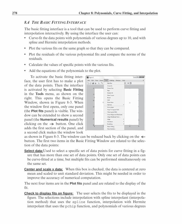
278 Chapter 8: Polynomials, Curve Fitting, and Interpolation
8.4 THE BASIC FITTING INTERFACE
The basic fitting interface is a tool that can be used to perform curve fitting andinterpolation interactively. By using the interface the user can:• Curve-fit the data points with polynomials of various degrees up to 10, and with
spline and Hermite interpolation methods.
• Plot the various fits on the same graph so that they can be compared.
• Plot the residuals of the various polynomial fits and compare the norms of theresiduals.
• Calculate the values of specific points with the various fits.
• Add the equations of the polynomials to the plot.
To activate the basic fitting inter-face, the user first has to make a plotof the data points. Then the interfaceis activated by selecting Basic Fittingin the Tools menu, as shown on theright. This opens the Basic FittingWindow, shown in Figure 8-3. Whenthe window first opens, only one panel(the panel) is visible. The win-dow can be extended to show a secondpanel (the panel) byclicking on the button. One clickadds the first section of the panel, anda second click makes the window lookas shown in Figure 8-3. The window can be reduced back by clicking on the button. The first two items in the Basic Fitting Window are related to the selec-tion of the data points:
Used to select a specific set of data points for curve fitting in a fig-ure that has more than one set of data points. Only one set of data points canbe curve-fitted at a time, but multiple fits can be performed simultaneously onthe same set.
When this box is checked, the data is centered at zeromean and scaled to unit standard deviation. This might be needed in order toimprove the accuracy of numerical computation.
The next four items are in the panel and are related to the display of thefit.
The user selects the fits to be displayed in thefigure. The selections include interpolation with spline interpolant (interpola-tion method) that uses the spline function, interpolation with Hermiteinterpolant that uses the pchip function, and polynomials of various degrees

8.4 The Basic Fitting Interface 279
that use the polyfit function. Several fits can be selected and displayedsimultaneously.
When this box is checked, the equations of the polynomialsthat were selected for the fit are displayed in the figure. The equations are dis-played with the number of significant digits selected in the adjacent signmenu.
When this box is checked, a plot that shows the residual at eachdata point is created (residuals are defined in Section 8.2.1). Choices in themenus include a bar plot, a scatter plot, and a line plot that can be displayedas a subplot in the same Figure Window that has the plot of the data points oras a separate plot in a different Figure Window.
When this box is checked, the norm of the residualsis displayed in the plot of the residuals. The norm of the residual is a measureof the quality of the fit. A smaller norm corresponds to a better fit.
The next three items are in the panel. They provide thenumerical information for one fit, independently of the fits that are displayed:
The user selects the fit to be examined numerically. The fit is shown on theplot only if it is selected in the panel.
Displays the numerical results for thepolynomial fit that is selected in the menu. It includes the coefficients ofthe polynomial and the norm of the residuals. The results can be saved by
Figure 8-3: The Basic Fitting Window.

280 Chapter 8: Polynomials, Curve Fitting, and Interpolation
clicking on the button.
Provides a means for obtaining interpolated (or extrapolated)numerical values for specified values of the independent variable. Enter thevalue of the independent variable in the box, and click on the but-ton. When the box is checked, the point is displayed onthe plot.
As an example, the basic fitting interface is used for fitting the data pointsfrom Sample Problem 8-3. The Basic Fitting Window is the one shown in Figure
8-3, and the corresponding Figure Window is shown in Figure 8-4. The FigureWindow includes a plot of the points, one interpolation fit (spline), two polyno-mial fits (linear and cubic), a display of the equations of the polynomial fits, anda mark of the point x = 1.5 that is entered in the box of the BasicFitting Window. The Figure Window also includes a plot of the residuals of thepolynomial fits and a display of their norm.
Figure 8-4: A Figure Window modified by the Basic Fitting Interface.
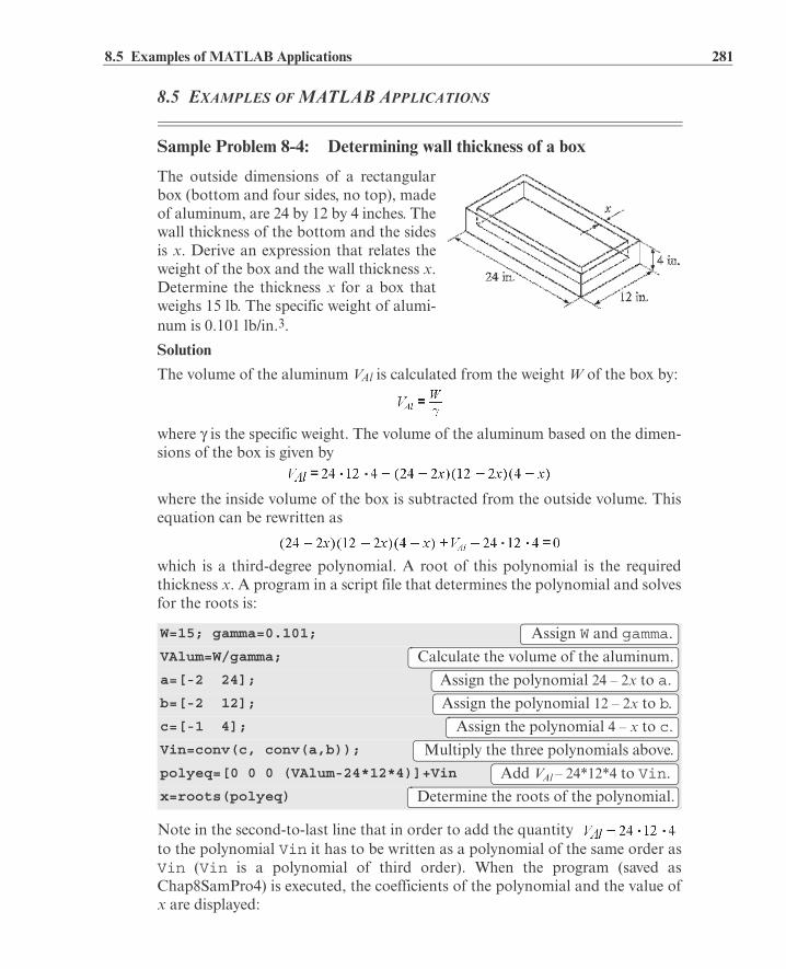
8.5 Examples of MATLAB Applications 281
8.5 EXAMPLES OF MATLAB APPLICATIONS
Sample Problem 8-4: Determining wall thickness of a box
The outside dimensions of a rectangularbox (bottom and four sides, no top), madeof aluminum, are 24 by 12 by 4 inches. Thewall thickness of the bottom and the sidesis x. Derive an expression that relates theweight of the box and the wall thickness x.Determine the thickness x for a box thatweighs 15 lb. The specific weight of alumi-num is 0.101 lb/in.3.
Solution
The volume of the aluminum VAl is calculated from the weight W of the box by:
where is the specific weight. The volume of the aluminum based on the dimen-sions of the box is given by
where the inside volume of the box is subtracted from the outside volume. Thisequation can be rewritten as
which is a third-degree polynomial. A root of this polynomial is the requiredthickness x. A program in a script file that determines the polynomial and solvesfor the roots is:
Note in the second-to-last line that in order to add the quantity to the polynomial Vin it has to be written as a polynomial of the same order asVin (Vin is a polynomial of third order). When the program (saved asChap8SamPro4) is executed, the coefficients of the polynomial and the value ofx are displayed:
W=15; gamma=0.101;
VAlum=W/gamma;
a=[-2 24];
b=[-2 12];
c=[-1 4];
Vin=conv(c, conv(a,b));
polyeq=[0 0 0 (VAlum-24*12*4)]+Vin
x=roots(polyeq)
Assign W and gamma.
Calculate the volume of the aluminum.
Assign the polynomial 24 – 2x to a.
Assign the polynomial 12 – 2x to b.
Assign the polynomial 4 – x to c.
Multiply the three polynomials above.
Add VAl – 24*12*4 to Vin.
Determine the roots of the polynomial.

282 Chapter 8: Polynomials, Curve Fitting, and Interpolation
Sample Problem 8-5: Floating height of a buoy
An aluminum thin-walled sphere is used as amarker buoy. The sphere has a radius of 60cm and a wall thickness of 12 mm. The den-sity of aluminum is kg/m3. Thebuoy is placed in the ocean, where the densityof the water is 1030 kg/m3. Determine theheight h between the top of the buoy and thesurface of the water.
Solution
According to Archimedes’s law, the buoyancyforce applied to an object that is placed in a fluid is equal to the weight of thefluid that is displaced by the object. Accordingly, the aluminum sphere will be ata depth such that the weight of the sphere is equal to the weight of the fluid dis-placed by the part of the sphere that is submerged.
The weight of the sphere is given by
where is the volume of the aluminum; and are the outside and insideradii of the sphere, respectively; and g is the gravitational acceleration.
The weight of the water that is displaced by the spherical portion that is sub-merged is given by:
Setting the two weights equal to each other gives the following equation:
The last equation is a third-degree polynomial for h. The root of the polynomialis the answer.
A solution with MATLAB is obtained by writing the polynomials and usingthe roots function to determine the value of h.This is done in the followingscript file:
>> Chap8SamPro4
polyeq = -4.0000 88.0000 -576.0000 148.5149
x = 10.8656 + 4.4831i 10.8656 - 4.4831i 0.2687
The polynomial is:.
The polynomial has one real root, x = 0.2687 in., which is the thickness of the aluminum
Al 2690=
VAl ro ri

8.5 Examples of MATLAB Applications 283
When the script file is executed in the Command Window, as shown below, theanswer is three roots, since the polynomial is of the third degree. The onlyanswer that is physically possible is the second, where h = 0.9029 m.
Sample Problem 8-6: Determining the size of a capacitor
An electrical capacitor has an unknowncapacitance. In order to determine itscapacitance, the capacitor is connected tothe circuit shown. The switch is first con-nected to B and the capacitor is charged.Then, the switch is connected to A and thecapacitor discharges through the resistor.As the capacitor is discharging, the voltage across the capacitor is measured for10 s in intervals of 1 s. The recorded measurements are given in the table below.Plot the voltage as a function of time and determine the capacitance of thecapacitor by fitting an exponential curve to the data points.
Solution
When a capacitor discharges through a resistor, the voltage of the capacitor as afunction of time is given by
where is the initial voltage, R the resistance of the resistor, and C the capaci-tance of the capacitor. As was explained in Section 8.2.2 the exponential func-tion can be written as a linear equation for ln(V) and t in the form:
rout=0.60; rin=0.588;
rhoalum=2690; rhowtr=1030;
a0=4*rout^3-4*rhoalum*(rout^3-rin^3)/rhowtr;
p = [1 -3*rout 0 a0];
h = roots(p)
>> Chap8SamPro5
h = 1.4542 0.9029 -0.5570
t (s) 1 2 3 4 5 6 7 8 9 10
V (V) 9.4 7.31 5.15 3.55 2.81 2.04 1.26 0.97 0.74 0.58
Assign the radii to variables.
Assign the densities to variables.
Assign the coefficient a0.
Assign the coefficient vector of the polynomial.
Calculate the roots of the polynomial.
The polynomial has three roots. The only one thatis physically possible for the problem is 0.9029 m.
V0

284 Chapter 8: Polynomials, Curve Fitting, and Interpolation
This equation, which has the form , can be fitted to the data pointsby using the polyfit(x,y,1) function with t as the independent variable xand ln(V) as the dependent variable y. The coefficients m and b determined bythe polyfit function are then used to determine C and by:
and
The following program written in a script file determines the best-fit exponentialfunction to the data points, determines C and , and plots the points and thefitted function.
When the script file is executed (saved as Chap8SamPro6) the values of C and are displayed in the Command Window as shown below:
The program creates also the following plot (axis labels were added to the plotusing the Plot Editor):
R=2000;
t=1:10;
v=[9.4 7.31 5.15 3.55 2.81 2.04 1.26 0.97 0.74 0.58];
p=polyfit(t,log(v),1);
C=-1/(R*p(1))
V0=exp(p(2))
tplot=0:0.1:10;
vplot=V0*exp(-tplot./(R*C));
plot(t,v,'o',tplot,vplot)
>> Chap8SamPro6
C = 0.0016
V0 = 13.2796
y mx b+=
V0
V0 eb=
V0
Define R.
Assign the data points to vectors t and v.
Use the polyfit function with t and log(v).
Calculate C from p(1), which is m in the equation.
Calculate V0 from p(2), which is b in the equation.
Create vector tplot of time for plotting the function.
Create vector vplot for plotting the function.
V0
The capacitance of the capacitor is 1,600 F.
t (s)0 2 4 6 8 10
V (
V)
0
2
4
6
8
10
12
14

8.5 Examples of MATLAB Applications 285
Sample Problem 8-7: Temperature dependence of viscosity
Viscosity, , is a property of gases and fluids that characterizes their resistanceto flow. For most materials, viscosity is highly sensitive to temperature. Below isa table that gives the viscosity of SAE 10W oil at different temperatures (datafrom B.R. Munson, D.F. Young, and T.H. Okiishi, Fundamentals of FluidMechanics, 4th ed., John Wiley and Sons, 2002). Determine an equation thatcan be fitted to the data.
Solution
To determine what type of equationmight provide a good fit to the data,
is plotted as a function of T (abso-lute temperature) with a linear scalefor T and a logarithmic scale for .The plot, shown on the right, indi-cates that the data points do notappear to line up along a straightline. This means that a simple expo-nential function of the form
, which models a straightline with these axes, will not providethe best fit. Since the points in the figure appear to lie along a curved line, afunction that can possibly have a good fit to the data is:
This function can be fitted to the data by using MATLAB’s polyfit(x,y,2)function (second-degree polynomial), where the independent variable is T andthe dependent variable is ln( ). The equation above can be solved for to givethe viscosity as a function of temperature:
The following program determines the best fit to the function and creates a plotthat displays the data points and the function.
T (°C) –20 0 20 40 60 80 100 120
(N s/m2)
( )4 0.38 0.095 0.032 0.015 0.007
80.004
50.003
2
T=[-20:20:120];
mu=[4 0.38 0.095 0.032 0.015 0.0078 0.0045 0.0032];
TK=T+273;
p=polyfit(TK,log(mu),2)
Temperature (K)250 300 350 400
Vis
cosi
ty (
N*s
/m2 )
10-3
10-2
10-1
100
101
y bemx=
ln a2T2 a1T a0+ +=
ea2T2 a1T a0+ +
ea0e
a1Te
a2T2
= =

286 Chapter 8: Polynomials, Curve Fitting, and Interpolation
When the program executes (saved as Chap8SamPro7), the coefficients that aredetermined by the polyfit function are displayed in the Command Window(shown below) as three elements of the vector p.
With these coefficients the viscosity of the oil as a function of temperature is:
The plot that is generated shows that the equation correlates well to the datapoints (axis labels were added with the Plot Editor).
8.6 PROBLEMS
1. Plot the polynomial in the domain. First create a vector for x, next use the polyval function to
calculate y, and then use the plot function.
2. Plot the polynomial in the domain .First create a vector for x, next use the polyval function to calculate y, andthen use the plot function.
3. Determine the polynomial that has roots at , ,, and . Make a plot of the polynomial in the domain
.
Tplot=273+[-20:120];
muplot = exp(p(1)*Tplot.^2 + p(2)*Tplot + p(3));
semilogy(TK,mu,'o',Tplot,muplot)
>> Chap8SamPro7
p = 0.0003 -0.2685 47.1673
Temperature (K)250 300 350 400
Vis
cosi
ty (
N*s
/m2 )
10-3
10-2
10-1
100
101

8.6 Problems 287
4. Use MATLAB to carry out the following multiplication of two polynomi-als:
5. Use MATLAB to carry out the following multiplication of polynomials:
Plot the polynomial in the domain .
6. Use MATLAB to divide the polynomial by the polynomial .
7. Use MATLAB to divide the polynomial by the polynomial
.
8. The product of four consecutive even integers is 1,488,384. Using MAT-LAB’s built-in function for operations with polynomials, determine the twointegers.
9. The product of three integers with spacing of 3 between them (e.g., 9, 12, 15)is 11,960. Using MATLAB’s built-in functions for operations with polyno-mials, determine the three integers.
10. The product of three distinct integers is 6,240. The sum of the numbers is85. The difference between the largest and the smallest is 57. Using MAT-LAB’s built-in functions for operations with polynomials, determine thethree integers.
11. A rectangular steel container (no top) has theoutside dimensions shown in the figure. Thethickness of the bottom surface is t, and thethickness of side walls is . Determine t ifthe weight of the container is 1,300 lb. Thespecific weight of steel is 0.284 lb/in.3.
240 in.
80 in.
120 in.

288 Chapter 8: Polynomials, Curve Fitting, and Interpolation
12. An aluminum container has the geometryshown in the figure (the bottom part is a rect-angular box and the top is half a cylinder). Theoutside dimensions are shown. The wall thick-ness of the bottom and all the vertical walls is2t, and the walls thickness of the cylindricalsection is t. Determine t if the tank weight is 30lb. The specific weight of aluminum is 0.101 lb/in.3.
13. A rectangular box (no top) is welded together usingsheet metal. The length of the box’s base is 18 in. longerthan its width. The total surface area of the sheet metal
that is used is 2,500 in.2.(a) Using polynomials write an expression for the vol-
ume V in terms of x.(b) Make a plot of V versus x for in.(c) Determine the dimensions of the box that maxi-
mizes the volume and determine that volume.
14. The probability P of selecting three distinct numbers out of n numbers iscalculated by:
Determine how many numbers, n, should be in a lottery game such that theprobability of matching three numbers out of n numbers will be at least 1/100,000, but not greater than 1/95,000.
15. Write a user-defined function that adds or subtracts two polynomials of anyorder. Name the function p=polyadd(p1,p2,operation). The firsttwo input arguments p1 and p2 are the vectors of the coefficients of the twopolynomials. (If the two polynomials are not of the same order, the functionadds the necessary zero elements to the shorter vector.) The third inputargument operation is a string that can be either ‘add’ or ‘sub’, foradding or subtracting the polynomials, respectively, and the output argu-ment is the resulting polynomial.
Use the function to add and subtract the following polynomials:
and
16. Write a user-defined function that multiplies two polynomials. Name thefunction p=polymult(p1,p2). The two input arguments p1 and p2 arevectors of the coefficients of the two polynomials. The output argument p isthe resulting polynomial.
Use the function to multiply the following polynomials:
24 in.
12 in.
10 in.
xx+18
h

8.6 Problems 289
and Check the answer with MATLAB’s built-in function conv.
17. Write a user-defined function that calculates the maximum (or minimum) ofa quadratic equation of the form:
Name the function [x,y,w] = maxormin(a,b,c). The input argumentsare the coefficients a, b, and c. The output arguments are x, the coordinateof the maximum (or minimum); y, the maximum (or minimum) value; andw, which is equal to 1 if y is a maximum and equal to 2 if y is a minimum.
Use the function to determine the maximum or minimum of the follow-ing functions:(a) (b)
18. A cylinder with base radius r and height h is con-structed inside a sphere such that it is in contactwith the surface of a sphere, as shown in the fig-ure. The radius of the sphere is in.(a) Create a polynomial expression for the vol-
ume V of the cylinder in terms of h.(b) Make a plot of V versus h for in.(c) Using the roots command determine h if
the volume of the cylinder is 2,000 in.3.(d) Determine the value of h that corresponds to the cylinder with the larg-
est possible volume, and determine that volume.
19. Consider the parabola:
, and the point .
(a) Write a polynomial expres-sion for the distance d frompoint P to an arbitrary point Qon the parabola.
(b) Make a plot of d versus y for.
(c) Determine the coordinates of Q if (there are two points).(d) Determine the coordinates of Q that correspond to the smallest d, and
calculate the corresponding value of d.(e) Make a plot that shows the parabola, point P, the two points from part
(c), and the point from part (d).
f x ax2 bx c+ +=
R
r
hR 11=
0 2 4 6 8 10 12-1
0
1
2
3
4
5P (3,4)
x
yQ
d
P 3 4,
d 3=

290 Chapter 8: Polynomials, Curve Fitting, and Interpolation
20. The following data is given:
(a) Use linear least-squares regression to determine the coefficients m and b inthe function that best fits the data.
(b) Make a plot that shows the function and the data points.
21. The boiling temperature of water at various altitudes h is given in thefollowing table. Determine a linear equation in the form thatbest fits the data. Use the equation for calculating the boiling temperatureat 5,000 m. Make a plot of the points and the equation.
22. The U.S. population in selected years between 1815 and 1965 is listed in thetable below. Determine a quadratic equation in the form
, where t is the number of years after 1800 and P is thepopulation in millions, that best fits the data. Use the equation to estimatethe population in 1915 (the population was 98.8 millions). Make a plot ofthe population versus the year that shows the data points and the equation.
23. The number of bacteria measured at different times t is given in the fol-lowing table. Determine an exponential function in the form that best fits the data. Use the equation to estimate the number of bacteriaafter 5 h. Make a plot of the points and the equation.
24. Growth data of a sunflower plant is given in the following table:
x –5 –4 –1 1 4 6 9 10y 12 10 6 2 –3 –6 –11 –12
h (ft) –1,000 0 3,000 8,000 15,000 22,000 28,000
T ( °F ) 213.9 212 206.2 196.2 184.4 172.6 163.1
Year 1815 1845 1875 1905 1935 1965
Population(millions)
8.3 19.7 44.4 83.2 127.1 190.9
t (h) 0 1 3 4 6 7 9
NB 500 600 1,000 1,400 2,100 2,700 4,100
Day 7 21 35 49 63 77 91
Height (in.) 8.5 21 50 77 89 98 99
y mx b+=
TB
TB mh b+=
P a2t2 a1t a0+ +=
NB
NB Ne t=

8.6 Problems 291
The data can be modeled with a function in the form , where y
is the height, H is a maximum height, a and b are constants, and t is thenumber of days. By using the method described in Section 8.2.2, and assum-ing that in., determine the constants a and b such that the functionbest fits the data. Use the function to estimate the height in day 40. In onefigure, plot the function and the data points.
25. Use the growth data from Problem 24 for the following:(a) Curve-fit the data with a third-order polynomial. Use the polynomial to
estimate the height in day 40. (b) Fit the data with linear and spline interpolations and use each interpo-
lation to estimate the height in day 40.
In each part make a plot of the data points (circle markers) and the fittedcurve or the interpolated curves. Note that part (b) has two interpolationcurves.
26. The following points are given:
(a) Fit the data with a first-order polynomial. Make a plot of the points andthe polynomial.
(b) Fit the data with a second-order polynomial. Make a plot of the pointsand the polynomial.
(c) Fit the data with a third-order polynomial. Make a plot of the pointsand the polynomial.
(d) Fit the data with an fifth-order polynomial. Make a plot of the pointsand the polynomial.
27. The standard air density, D (average of measurements made), at differentheights, h, from sea level up to a height of 33 km is given below.
(a) Make the following four plots of the data points (density as a functionof height): (1) both axes with linear scale; (2) h with log axis, D with lin-ear axis; (3) h with linear axis, D with log axis; (4) both log axes. Accord-ing to the plots, choose a function (linear, power, exponential, or
x 1 2.2 3.7 6.4 9 11.5 14.2 17.8 20.5 23.2
y 12 9 6.6 5.5 7.2 9.2 9.6 8.5 6.5 2.2
h (km) 0 3 6 9 12 15
D (kg/m3) 1.2 0.91 0.66 0.47 0.31 0.19
h (km) 18 21 24 27 30 33
D (kg/m3) 0.12 0.075 0.046 0.029 0.018 0.011
H 102=

292 Chapter 8: Polynomials, Curve Fitting, and Interpolation
logarithmic) that best fits the data points and determine the coefficientsof the function.
(b) Plot the function and the points using linear axes.
28. Write a user-defined function that determines the best fit of an exponentialfunction of the form . Name the function [b,m] =expofit(x,y), where the input arguments x and y are vectors with thecoordinates of the data points, and the output arguments b and m are theconstants of the fitted exponential equation. Use expofit to fit the databelow. Make a plot that shows the data points and the function.
29. Estimated values of thermal conductivity of silicon at different temperaturesare given in the following table.
(a) Make a plot of k versus T using log scale on both axes.
(b) Curve-fit the data with a second-order polynomial inwhich and . Once the coefficients a, b, and c aredetermined, write an equation for k as a function of . Use thisequation for curve-fitting the data. Make a second plot that shows thedata points with markers and the curve-fitted equation with a solid line.
(c) Repeat part (b) using a third-order polynomial.
30. Measurements of the concentration, C, of a substance during a chemicalreaction at different times t are shown in the table.
(a) Suppose that the data can be modeled with an equation in the form:
Determine the coefficients a0, a1, and a2 such that the equation best fitsthe data. Use the equation to estimate the concentration at h.
x 0.4 2.2 3.1 5.0 6.6 7.6
y 1.7 10.1 26.9 61.2 158 398
T (K) 2 4 6 8 10 20 40 60
k (W/m-K) 46 300 820 1,560 2,300 5,000 3,500 2,100
T (K) 80 100 150 250 350 500 1,000 1,400
k (W/m-K) 1,350 900 400 190 120 75 30 20
t (h) 0.5 1.0 1.5 2.0 2.5 3.0 3.5 4.0 4.5 5.0 5.5 6.0
C (g/L) 1.7 3.1 5.7 9.1 6.4 3.7 2.8 1.6 1.2 0.8 0.7 0.6
8.6 Problems 293
Make a plot of the data points and the equation.(b) Suppose that the data can be modeled with an equation in the form:
Determine the coefficients a0, a1, a2, and a3 such that the equation bestfits the data. Use the equation to estimate the concentration at h.Make a plot of the data points and the equation.
31. Use the data from Problem 30 for the following:(a) Fit the data with linear interpolation. Estimate the concentration at
. Make a plot that shows the data points and curve made ofinterpolated points.
(b) Fit the data with spline interpolation. Estimate the concentration ath. Make a plot that shows the data points and a curve made of
interpolated points.
32. The relationship between two variables y and x is known to be:
The following data points are given:
Determine the constants a and b by curve-fitting the equation to the datapoints. Make a plot of y versus x. In the plot show the data points withmarkers and the curve-fitted equation with a solid line. Use the equation toestimate y at . (The curve fitting can be done by writing the reciprocalof the equation and using a first-order polynomial.)
33. Curve-fit the data from the previous problem with a third-order polynomial.Use the polynomial to estimate y at . Make a plot of the points andthe polynomial.
34. When rubber is stretched, its elongation is initially proportional to theapplied force, but as it reaches about twice its original length, the forcerequired to stretch the rubber increases rapidly. The force, as a function ofelongation, that was required to stretch a rubber specimen that was initially3 in. long is displayed in the following table.(a) Curve-fit the data with a fourth-order polynomial. Make a plot of the
data points and the polynomial. Use the polynomial to estimate theforce when the rubber specimen was 11.5 in. long.
(b) Fit the data with spline interpolation (use MATLAB’s built-in functioninterp1). Make a plot that shows the data points and a curve made byinterpolation. Use interpolation to estimate the force when the rubber
x 5 10 15 20 25 30 35 40 45 50y 15 25 32 33 37 35 38 39 41 42
y ax
b x+-------------=

294 Chapter 8: Polynomials, Curve Fitting, and Interpolation
specimen was 11.5 in. long.
35. The transmission of light through a transparent solid can be described bythe equation:
where is the transmitted intensity, is the intensity of the incidentbeam, is the absorption coefficient, L is the length of the transparent solid,and R is the fraction of light which is reflected at the interface. If the light isnormal to the interface and the beams are transmitted through air,
where n is the index of refraction for the transparent solid.
Experiments measuring the intensity of light transmitted through specimensof a transparent solid of various lengths are given in the following table. The
intensity of the incident beam is 5 W/m2.
Use this data and curve fitting to determine the absorption coefficient andindex of refraction of the solid.
Force (lb) 0 0.6 0.9 1.16 1.18 1.19 1.24 1.48Elongation (in.) 0 1.2 2.4 3.6 4.8 6.0 7.2 8.4
Force (lb) 1.92 3.12 4.14 5.34 6.22 7.12 7.86 8.42Elongation (in.) 9.6 10.8 12.0 13.2 14.4 15.6 16.8 18
L (cm) 0.5 1.2 1.7 2.2 4.5 6.0
(W/m2) 4.2 4.0 3.8 3.6 2.9 2.5
IT I0
IT

295
Chapter 9 Applications in Numerical Analysis
Numerical methods are commonly used for solving mathematical problems thatare formulated in science and engineering where it is difficult or impossible toobtain exact solutions. MATLAB has a large library of functions for numeri-cally solving a wide variety of mathematical problems. This chapter explains anumber of the most frequently used of these functions. It should be pointed outhere that the purpose of this book is to show users how to use MATLAB. Somegeneral information on the numerical methods is given, but the details, whichcan be found in books on numerical analysis, are not included.
The following topics are presented in this chapter: solving an equation withone unknown, finding a minimum or a maximum of a function, numerical inte-gration, and solving a first-order ordinary differential equation.
9.1 SOLVING AN EQUATION WITH ONE VARIABLE
An equation with one variable can be written in the form . A solutionto the equation (also called a root) is a numerical value of x that satisfies theequation. Graphically, a solution is a point where the function crosses ortouches the x axis. An exact solution is a value of x for which the value of thefunction is exactly zero. If such a value does not exist or is difficult to determine,a numerical solution can be determined by finding an x that is very close to thesolution. This is done by the iterative process, where in each iteration the com-puter determines a value of x that is closer to the solution. The iterations stopwhen the difference in x between two iterations is smaller than some measure. Ingeneral, a function can have zero, one, several, or an infinite number of solu-tions.
f x 0=
f x

296 Chapter 9: Applications in Numerical Analysis
In MATLAB a zero of a function can be determined with the command(built-in function) fzero with the form:
The built-in function fzero is a MATLAB function function (see Section 7.9),which means that it accepts another function (the function to be solved) as aninput argument.
Additional details on the arguments of fzero:
• x is the solution, which is a scalar.
• function is the function to be solved. It can be entered in several differentways:1. The simplest way is to enter the mathematical expression as a string.2. The function is created as a user-defined function in a function file and then the function handle is entered (see Section 7.9.1). 3. The function is created as an anonymous function (see Section 7.8.1) and then the name of the anonymous function (which is the name of the handle) is entered (see Section 7.9.1).
(As explained in Section 7.9.2, it is also possible to pass a user-defined functionand an inline function into a function function by using its name. However,function handles are more efficient and easier to use, and should be the preferredmethod.)
• The function has to be written in a standard form. For example, if the functionto be solved is , it has to be written as . If thisfunction is entered into the fzero command as a string, it is typed as:‘x*exp(-x)-0.2’.
• When a function is entered as an expression (string), it cannot include pre-defined variables. For example, if the function to be entered is ,it is not possible to define b=0.2 and then enter ‘x*exp(-x)-b’.
• x0 can be a scalar or a two-element vector. If it is entered as a scalar, it has to bea value of x near the point where the function crosses (or touches) the x axis. Ifx0 is entered as a vector, the two elements have to be points on opposite sides ofthe solution. If crosses the x axis, then has a different sign than
. When a function has more than one solution, each solution can bedetermined separately by using the fzero function and entering values for x0that are near each of the solutions.
x = fzero(function,x0)
Solution The function to be solved.
A value of x close to where the function crosses the axis.
f x f x0 1
f x0 2
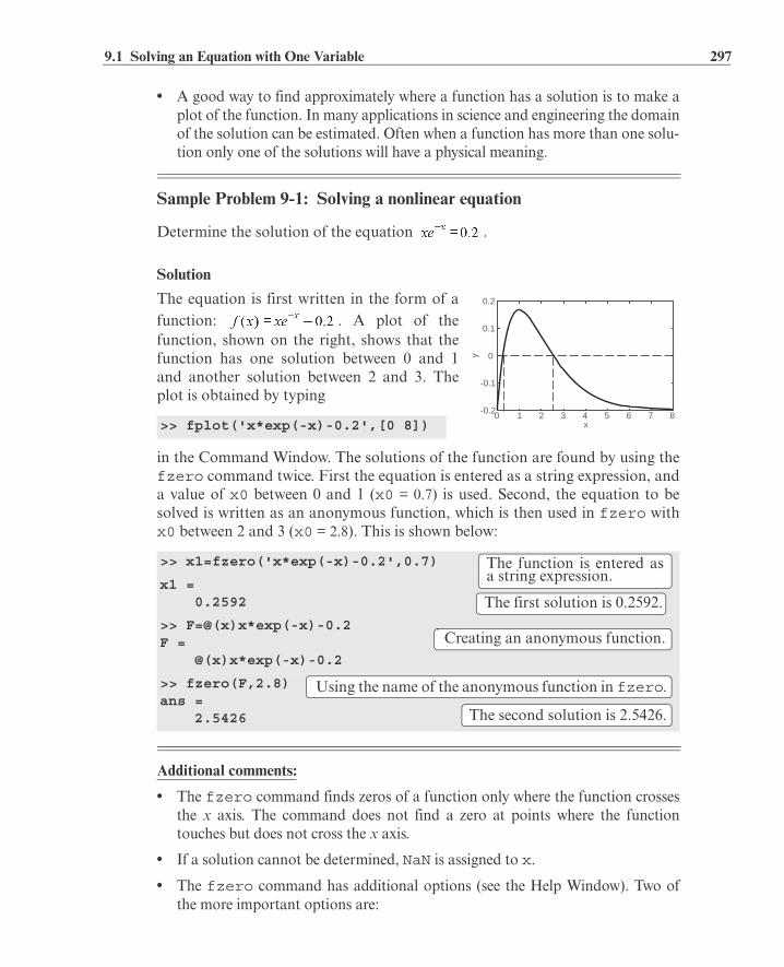
9.1 Solving an Equation with One Variable 297
• A good way to find approximately where a function has a solution is to make aplot of the function. In many applications in science and engineering the domainof the solution can be estimated. Often when a function has more than one solu-tion only one of the solutions will have a physical meaning.
Sample Problem 9-1: Solving a nonlinear equation
Determine the solution of the equation .
Solution
The equation is first written in the form of afunction: . A plot of thefunction, shown on the right, shows that thefunction has one solution between 0 and 1and another solution between 2 and 3. Theplot is obtained by typing
in the Command Window. The solutions of the function are found by using thefzero command twice. First the equation is entered as a string expression, anda value of x0 between 0 and 1 (x0 = 0.7) is used. Second, the equation to besolved is written as an anonymous function, which is then used in fzero withx0 between 2 and 3 (x0 = 2.8). This is shown below:
Additional comments:
• The fzero command finds zeros of a function only where the function crossesthe x axis. The command does not find a zero at points where the functiontouches but does not cross the x axis.
• If a solution cannot be determined, NaN is assigned to x.
• The fzero command has additional options (see the Help Window). Two ofthe more important options are:
>> fplot('x*exp(-x)-0.2',[0 8])
>> x1=fzero('x*exp(-x)-0.2',0.7)
x1 = 0.2592
>> F=@(x)x*exp(-x)-0.2F = @(x)x*exp(-x)-0.2
>> fzero(F,2.8)ans = 2.5426
x0 1 2 3 4 5 6 7 8
y
-0.2
-0.1
0
0.1
0.2
The function is entered asa string expression.
The first solution is 0.2592.
Creating an anonymous function.
Using the name of the anonymous function in fzero.
The second solution is 2.5426.

298 Chapter 9: Applications in Numerical Analysis
[x fval]=fzero(function, x0) assigns the value of the function at x tothe variable fval.x=fzero(function, x0, optimset(‘display’,‘iter’)) displaysthe output of each iteration during the process of finding the solution.
• When the function can be written in the form of a polynomial, the solution, orthe roots, can be found with the roots command, as explained in Chapter 8(Section 8.1.2).
• The fzero command can also be used to find the value of x where the functionhas a specific value. This is done by translating the function up or down. Forexample, in the function of Sample Problem 9-1 the first value of x where thefunction is equal to 0.1 can be determined by solving the equation
. This is shown below:
9.2 FINDING A MINIMUM OR A MAXIMUM OF A FUNCTION
In many applications there is a need to determine the local minimum or maxi-mum of a function of the form . In calculus the value of x that corre-sponds to a local minimum or maximum is determined by finding the zero ofthe derivative of the function. The value of y is determined by substituting the xinto the function. In MATLAB the value of x where a one-variable function
within the interval has a minimum can be determined with thefminbnd command which has the form:
• The function can be entered as a string expression, or as a function handle, inthe same way as with the fzero command. See Section 9.1 for details.
• The value of the function at the minimum can be added to the output by usingthe option [x fval]=fminbnd(function,x1,x2)
where the value of the function at x is assigned to the variable fval.
• Within a given interval, the minimum of a function can either be at one of theend points of the interval or at a point within the interval where the slope of thefunction is zero (local minimum). When the fminbnd command is executed,MATLAB looks for a local minimum. If a local minimum is found, its value is
>> x=fzero('x*exp(-x)-0.3',0.5)
x = 0.4894
y f x=
f x
x = fminbnd(function,x1,x2)
The value of x where the function has a minimum.
The function. The interval of x.

9.2 Finding a Minimum or a Maximum of a Function 299
compared to the value of the function at the end points of the interval. MAT-LAB returns the point with the actual minimum value for the interval.
For example, consider the function
, which is plot-ted in the interval in the figure onthe right. It can be observed that there is alocal minimum between 5 and 6, and that theabsolute minimum is at . Using thefminbnd command with the interval
to find the location of the local min-imum and the value of the function at this point gives:
Notice that the fminbnd command gives the local minimum. If the interval ischanged to , fminbnd gives:
For this interval the fminbnd command gives the absolute minimum which isat the end point .• The fminbnd command can also be used to find the maximum of a function.
This is done by multiplying the function by –1 and finding the minimum. Forexample, the maximum of the function (from Sample Problem9-1) in the interval can be determined by finding the minimum of thefunction as shown below:
>> [x fval]=fminbnd('x^3-12*x^2+40.25*x-36.5',3,8)
x = 5.6073fval = -11.8043
>> [x fval]=fminbnd('x^3-12*x^2+40.25*x-36.5',0,8)
x = 0fval = -36.5000
>> [x fval]=fminbnd('-x*exp(-x)+0.2',0,8)
x = 1.0000fval = -0.1679
x0 1 2 3 4 5 6 7 8
f(x)
-40
-30
-20
-10
0
10
20
30
x 0=
The local minimum is at . The value of the function at this point is –11.8043.
x 5.6073=
The minimum is at . The value of the function at this point is –36.5.
x 0=
x 0=
The maximum is at x = 1.0. The value ofthe function at this point is 0.1679.
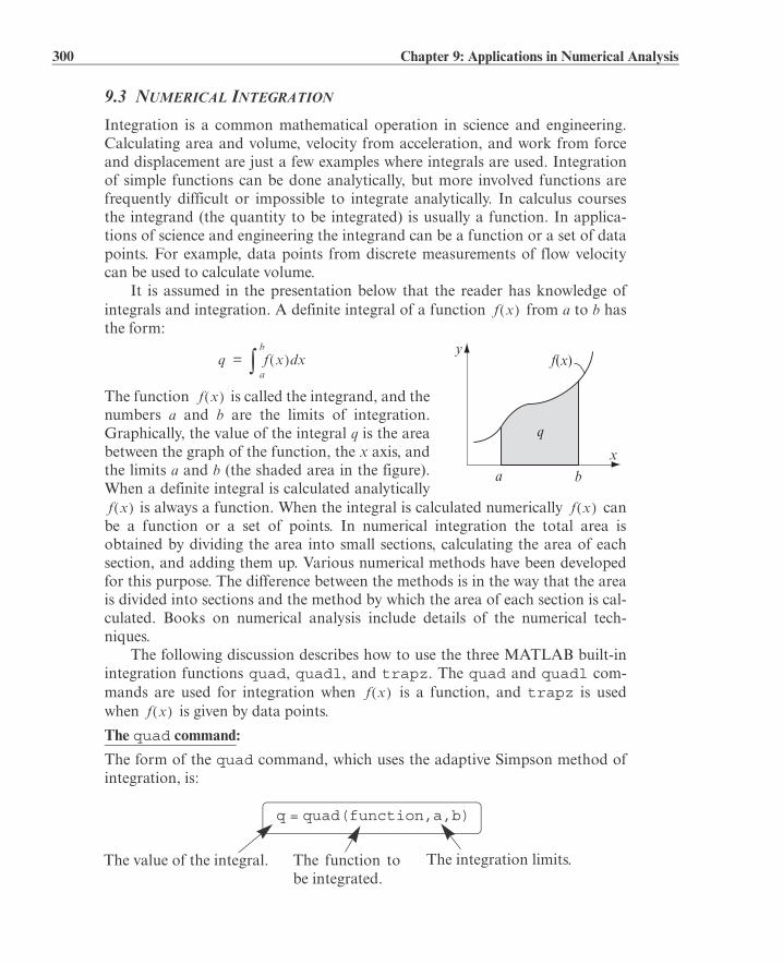
300 Chapter 9: Applications in Numerical Analysis
9.3 NUMERICAL INTEGRATION
Integration is a common mathematical operation in science and engineering.Calculating area and volume, velocity from acceleration, and work from forceand displacement are just a few examples where integrals are used. Integrationof simple functions can be done analytically, but more involved functions arefrequently difficult or impossible to integrate analytically. In calculus coursesthe integrand (the quantity to be integrated) is usually a function. In applica-tions of science and engineering the integrand can be a function or a set of datapoints. For example, data points from discrete measurements of flow velocitycan be used to calculate volume.
It is assumed in the presentation below that the reader has knowledge ofintegrals and integration. A definite integral of a function from a to b hasthe form:
The function is called the integrand, and thenumbers a and b are the limits of integration.Graphically, the value of the integral q is the areabetween the graph of the function, the x axis, andthe limits a and b (the shaded area in the figure).When a definite integral is calculated analytically
is always a function. When the integral is calculated numerically canbe a function or a set of points. In numerical integration the total area isobtained by dividing the area into small sections, calculating the area of eachsection, and adding them up. Various numerical methods have been developedfor this purpose. The difference between the methods is in the way that the areais divided into sections and the method by which the area of each section is cal-culated. Books on numerical analysis include details of the numerical tech-niques.
The following discussion describes how to use the three MATLAB built-inintegration functions quad, quadl, and trapz. The quad and quadl com-mands are used for integration when is a function, and trapz is usedwhen is given by data points.
The quad command:
The form of the quad command, which uses the adaptive Simpson method ofintegration, is:
f x
x
f(x)
a b
q
yq f x xd
a
b=
f x
f x f x
f xf x
q = quad(function,a,b)
The value of the integral. The function tobe integrated.
The integration limits.
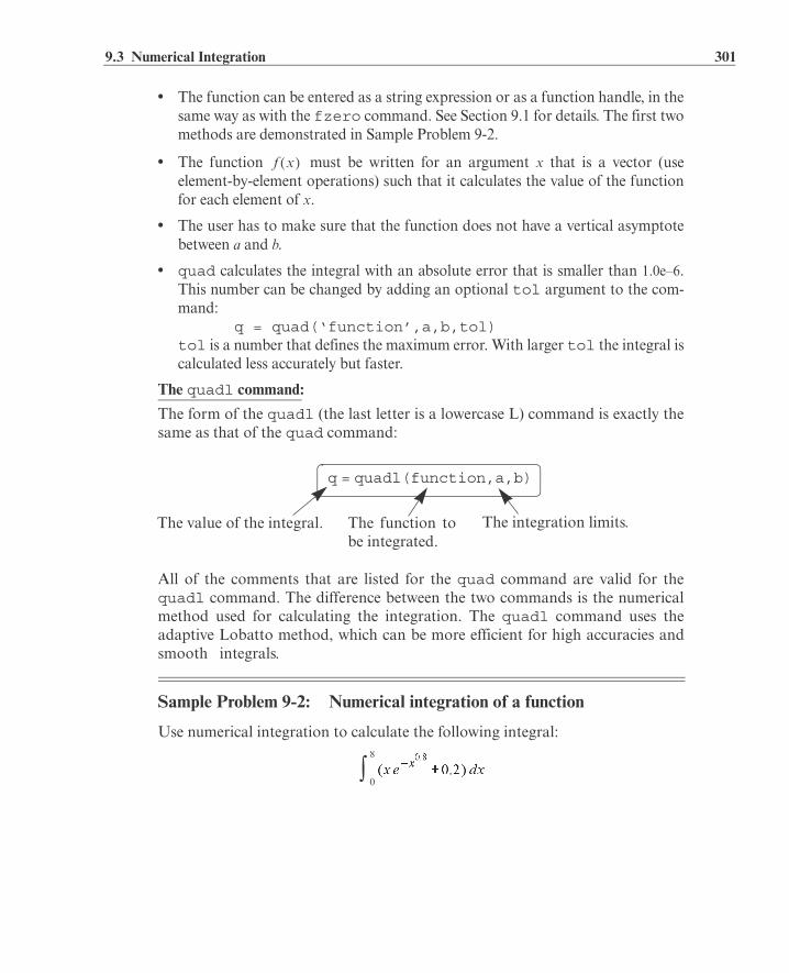
9.3 Numerical Integration 301
• The function can be entered as a string expression or as a function handle, in thesame way as with the fzero command. See Section 9.1 for details. The first twomethods are demonstrated in Sample Problem 9-2.
• The function must be written for an argument x that is a vector (useelement-by-element operations) such that it calculates the value of the functionfor each element of x.
• The user has to make sure that the function does not have a vertical asymptotebetween a and b.
• quad calculates the integral with an absolute error that is smaller than 1.0e–6.This number can be changed by adding an optional tol argument to the com-mand: q = quad(‘function’,a,b,tol)tol is a number that defines the maximum error. With larger tol the integral iscalculated less accurately but faster.
The quadl command:
The form of the quadl (the last letter is a lowercase L) command is exactly thesame as that of the quad command:
All of the comments that are listed for the quad command are valid for thequadl command. The difference between the two commands is the numericalmethod used for calculating the integration. The quadl command uses theadaptive Lobatto method, which can be more efficient for high accuracies andsmooth integrals.
Sample Problem 9-2: Numerical integration of a function
Use numerical integration to calculate the following integral:
f x
q = quadl(function,a,b)
The value of the integral. The function tobe integrated.
The integration limits.
0
8
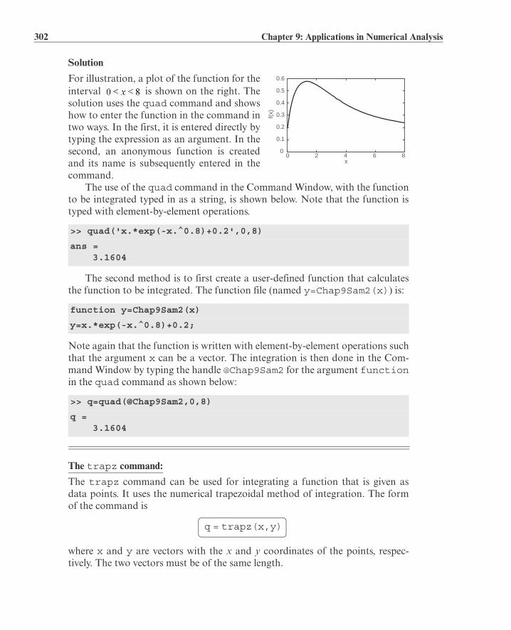
302 Chapter 9: Applications in Numerical Analysis
Solution
For illustration, a plot of the function for theinterval is shown on the right. Thesolution uses the quad command and showshow to enter the function in the command intwo ways. In the first, it is entered directly bytyping the expression as an argument. In thesecond, an anonymous function is createdand its name is subsequently entered in thecommand.
The use of the quad command in the Command Window, with the functionto be integrated typed in as a string, is shown below. Note that the function istyped with element-by-element operations.
The second method is to first create a user-defined function that calculatesthe function to be integrated. The function file (named y=Chap9Sam2(x)) is:
Note again that the function is written with element-by-element operations suchthat the argument x can be a vector. The integration is then done in the Com-mand Window by typing the handle @Chap9Sam2 for the argument functionin the quad command as shown below:
The trapz command:
The trapz command can be used for integrating a function that is given asdata points. It uses the numerical trapezoidal method of integration. The formof the command is
where x and y are vectors with the x and y coordinates of the points, respec-tively. The two vectors must be of the same length.
>> quad('x.*exp(-x.^0.8)+0.2',0,8)
ans = 3.1604
function y=Chap9Sam2(x)
y=x.*exp(-x.^0.8)+0.2;
>> q=quad(@Chap9Sam2,0,8)
q = 3.1604
x0 2 4 6 8
f(x)
0
0.1
0.2
0.3
0.4
0.5
0.6
q = trapz(x,y)

9.4 Ordinary Differential Equations 303
9.4 ORDINARY DIFFERENTIAL EQUATIONS
Differential equations play a crucial role in science and engineering since theyare in the foundation of virtually every physical phenomenon that is involved inengineering applications. Only a limited number of differential equations can besolved analytically. Numerical methods, on the other hand, can result in anapproximate solution to almost any equation. Obtaining a numerical solutionmight not be simple task however. This is because a numerical method that cansolve any equation does not exist. Instead, there are many methods that are suit-able for solving different types of equations. MATLAB has a large library oftools that can be used for solving differential equations. To fully utilize thepower of MATLAB, however, requires that the user have knowledge of differen-tial equations and the various numerical methods that can be used for solvingthem.
This section describes in detail how to use MATLAB to solve a first-orderordinary differential equation. The possible numerical methods that can be usedfor solving such an equation are described in general terms, but are notexplained from a mathematical point of view. This section provides informationfor solving simple, “nonproblematic” first-order equations. This solution pro-vides the basis for solving higher-order equations and systems of equations.
An ordinary differential equation (ODE) is an equation that contains anindependent variable, a dependent variable, and derivatives of the dependentvariable. The equations that are considered here are of first order with the form
where x and y are the independent and dependent variables, respectively. A solu-tion is a function that satisfies the equation. In general, many func-tions can satisfy a given ODE, and more information is required fordetermining the solution of a specific problem. The additional information isthe value of the function (the dependent variable) at some value of the indepen-dent variable.
Steps for solving a single first-order ODE:
For the remainder of this section the independent variable is taken as t (time).This is done because in many applications time is the independent variable, andalso to be consistent with the information in the Help menu of MATLAB.
Step 1:Write the problem in a standard form.
Write the equation in the form:
for , with at .
As shown above, three pieces of information are needed for solving a first orderODE: An equation that gives an expression for the derivative of y with respectto t, the interval of the independent variable, and the initial value of y. The solu-tion is the value of y as a function of t between and .
dydx------ f x y,=
y f x=
dydt------ f t y,= y y0= t t0=
t0 tf

304 Chapter 9: Applications in Numerical Analysis
An example of a problem to solve is:
for with at .
Step 2:Create a user-defined function (in a function file) or an anonymous function.The ODE to be solved has to be written as a user-defined function (in a function
file) or as an anonymous function. Both calculate for given values of t and y.
For the example problem above, the user-defined function (which is saved as aseparate file) is:
When an anonymous function is used, it can be defined in the Command Win-dow, or be within a script file. For the example problem here the anonymousfunction (named ode1) is:
Step 3:Select a method of solution.
Select the numerical method that you would like MATLAB to use in the solu-tion. Many numerical methods have been developed to solve first-order ODEs,and several of the methods are available as built-in functions in MATLAB. In atypical numerical method, the time interval is divided into small time steps. Thesolution starts at the known point y0, and then by using one of the integrationmethods the value of y is calculated at each time step. Table 9-1 lists seven ODEsolver commands, which are MATLAB built-in functions that can be used forsolving a first-order ODE. A short description of each solver is included in thetable.
function dydt=ODEexp1(t,y)
dydt=(t^3-2*y)/t;
>> ode1=@(t,y)(t^3-2*y)/tode1 = @(t,y)(t^3-2*y)/t
Table 9-1: MATLAB ODE Solvers
ODE Solver Name Description
ode45 For nonstiff problems, one-step solver, best toapply as a first try for most problems. Based onexplicit Runge-Kutta method.
ode23 For nonstiff problems, one-step solver. Based onexplicit Runge-Kutta method. Often quicker butless accurate than ode45.
ode113 For nonstiff problems, multistep solver.
y 4.2= t 1=
dydt------

9.4 Ordinary Differential Equations 305
In general, the solvers can be divided into two groups according to theirability to solve stiff problems and according to whether they use on-step or mul-tistep methods. Stiff problems are ones that include fast and slowly changingcomponents and require small time steps in their solution. One-step solvers useinformation from one point to obtain a solution at the next point. Multistepsolvers use information from several previous points to find the solution at thenext point. The details of the different methods are beyond the scope of thisbook.
It is impossible to know ahead of time which solver is the most appropriatefor a specific problem. A suggestion is to first try ode45, which gives goodresults for many problems. If a solution is not obtained because the problem isstiff, trying the solver ode15s is suggested.
Step 4: Solve the ODE.
The form of the command that is used to solve an initial value ODE problem isthe same for all the solvers and for all the equations that are solved. The form is:
Additional information:
solver_name Is the name of the solver (numerical method) that is used (e.g.ode45 or ode23s)
ODEfun The function from Step 2 that calculates for given values
of t and y. If it was written as a user-defined function, thefunction handle is entered. If it was written as an anonymousfunction, the name of the anonymous function is entered. (Seethe example that follows.)
tspan A vector that specifies the interval of the solution. The vectormust have at least two elements but can have more. If thevector has only two elements, the elements must be [t0 tf],which are the initial and final points of the solution interval.
ode15s For stiff problems, multistep solver. Use if ode45failed. Uses a variable order method.
ode23s For stiff problems, one-step solver. Can solve someproblems that ode15s cannot.
ode23t For moderately stiff problems.
ode23tb For stiff problems. Often more efficient thanode15s.
Table 9-1: MATLAB ODE Solvers (Continued)
ODE Solver Name Description
[t,y] = solver_name(ODEfun,tspan,y0)
dydt------

306 Chapter 9: Applications in Numerical Analysis
The vector tspan can have, however, additional pointsbetween the first and last points. The number of elements intspan affects the output from the command. See [t,y]below.
y0 The initial value of y (the value of y at the first point of theinterval).
[t,y] The output, which is the solution of the ODE. t and y arecolumn vectors. The first and the last points are the beginningand end points of the interval. The spacing and number ofpoints in between depends on the input vector tspan. Iftspan has two elements (the beginning and end points), thevectors t and y contain the solution at every integration stepcalculated by the solver. If tspan has more than two points(additional points between the first and the last), the vectors tand y contain the solution only at these points. The numberof points in tspan does not affect the time steps used for thesolution by the program.
For example, consider the solution to the problem stated in Step 1:
for with at ,
If the ODE function is written as a user-defined function (see Step 2), then thesolution with MATLAB’s built-in function ode45 is obtained by:
The solution is obtained with the solver ode45. The name of the user-definedfunction from Step 2 is ODEexp1. The solution starts at and ends at
with increments of 0.5 (according to the vector tspan). To show thesolution, the problem is solved again below using tspan with smaller spacing,
>> [t y]=ode45(@ODEexp1,[1:0.5:3],4.2)
t = 1.0000
1.5000
2.0000
2.5000
3.0000
y = 4.2000
2.4528
2.6000
3.7650
5.8444
y 4.2= t 1=
The handle of the user-defined function ODEexp1.
The initial value.
The vector tspan.
t 1=t 3=

9.5 Examples of MATLAB Applications 307
and the solution is plotted with the plot command.
If the ODE function is written as an anonymous function called ode1 (see Step2), then the solution (same as shown above) is obtained by typing:[t y]=ode45(ode1,[1:0.5:3],4.2)
9.5 EXAMPLES OF MATLAB APPLICATIONS
Sample Problem 9-3: The gas equation
The ideal gas equation relates the volume (V in L), temperature (T in K), pres-sure (P in atm), and the amount of gas (number of moles n) by:
where R = 0.08206 (L atm)/(mol K) is the gas constant.
The van der Waals equation gives the relationship between these quantitiesfor a real gas by
where a and b are constants that are specific for each gas.
Use the fzero function to calculate the volume of 2 mol CO2 at temperature of
50°C, and pressure of 6 atm. For CO2, a = 3.59 (L2 atm)/mol2, and b = 0.0427 L/mol.
Solution
The solution written in a script file is shown below.
>> [t y]=ode45(@ODEexp1,[1:0.01:3],4.2);
>> plot(t,y)
>> xlabel('t'), ylabel('y')
global P T n a b R
t1 1.5 2 2.5 3
y
22.5
33.5
44.5
55.5
6
pnRT
V------------=
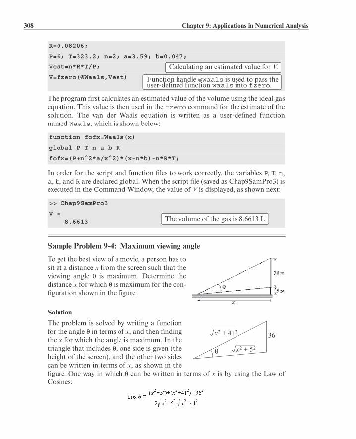
308 Chapter 9: Applications in Numerical Analysis
The program first calculates an estimated value of the volume using the ideal gasequation. This value is then used in the fzero command for the estimate of thesolution. The van der Waals equation is written as a user-defined functionnamed Waals, which is shown below:
In order for the script and function files to work correctly, the variables P, T, n,a, b, and R are declared global. When the script file (saved as Chap9SamPro3) isexecuted in the Command Window, the value of V is displayed, as shown next:
Sample Problem 9-4: Maximum viewing angle
To get the best view of a movie, a person has tosit at a distance x from the screen such that theviewing angle is maximum. Determine thedistance x for which is maximum for the con-figuration shown in the figure.
Solution
The problem is solved by writing a functionfor the angle in terms of x, and then findingthe x for which the angle is maximum. In thetriangle that includes , one side is given (theheight of the screen), and the other two sidescan be written in terms of x, as shown in thefigure. One way in which can be written in terms of x is by using the Law ofCosines:
R=0.08206;
P=6; T=323.2; n=2; a=3.59; b=0.047;
Vest=n*R*T/P;
V=fzero(@Waals,Vest)
function fofx=Waals(x)
global P T n a b R
fofx=(P+n^2*a/x^2)*(x-n*b)-n*R*T;
>> Chap9SamPro3
V = 8.6613
Calculating an estimated value for V.
Function handle @waals is used to pass the user-defined function waals into fzero.
The volume of the gas is 8.6613 L.
x2 52+
x2 412+ 36
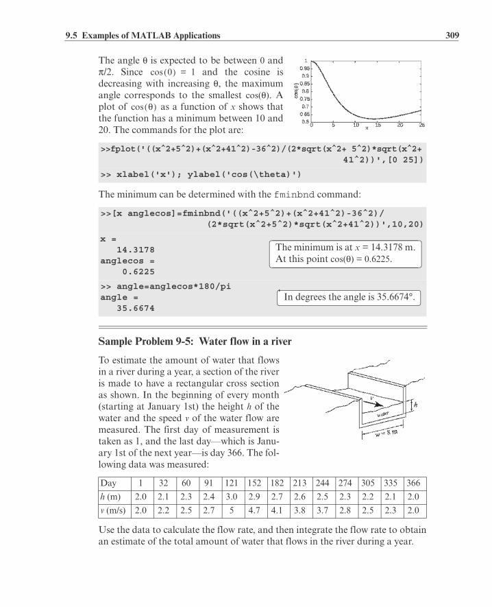
9.5 Examples of MATLAB Applications 309
The angle is expected to be between 0 and/2. Since and the cosine is
decreasing with increasing , the maximumangle corresponds to the smallest cos( ). Aplot of as a function of x shows thatthe function has a minimum between 10 and20. The commands for the plot are:
The minimum can be determined with the fminbnd command:
Sample Problem 9-5: Water flow in a river
To estimate the amount of water that flowsin a river during a year, a section of the riveris made to have a rectangular cross sectionas shown. In the beginning of every month(starting at January 1st) the height h of thewater and the speed v of the water flow aremeasured. The first day of measurement istaken as 1, and the last day—which is Janu-ary 1st of the next year—is day 366. The fol-lowing data was measured:
Use the data to calculate the flow rate, and then integrate the flow rate to obtainan estimate of the total amount of water that flows in the river during a year.
>>fplot('((x^2+5^2)+(x^2+41^2)-36^2)/(2*sqrt(x^2+ 5^2)*sqrt(x^2+ 41^2))',[0 25])
>> xlabel('x'); ylabel('cos(\theta)')
>>[x anglecos]=fminbnd('((x^2+5^2)+(x^2+41^2)-36^2)/ (2*sqrt(x^2+5^2)*sqrt(x^2+41^2))',10,20)
x = 14.3178anglecos = 0.6225
>> angle=anglecos*180/piangle = 35.6674
Day 1 32 60 91 121 152 182 213 244 274 305 335 366
h (m) 2.0 2.1 2.3 2.4 3.0 2.9 2.7 2.6 2.5 2.3 2.2 2.1 2.0
v (m/s) 2.0 2.2 2.5 2.7 5 4.7 4.1 3.8 3.7 2.8 2.5 2.3 2.0
0cos 1=
cos
The minimum is at x = 14.3178 m.At this point cos( ) = 0.6225.The minimum is at x = 14.3178 m.At this point cos( ) = 0.6225.The minimum is at x = 14.3178 m. At this point cos( ) = 0.6225.
In degrees the angle is 35.6674°.

310 Chapter 9: Applications in Numerical Analysis
Solution
The flow rate, Q (volume of water per second), at each data point is obtained bymultiplying the water speed by the width and height of the cross-sectional areaof the water that flows in the channel:
(m3/s)
The total amount of water that flows is estimated by the integral:
The flow rate is given in cubic meters per second, which means that time musthave units of seconds. Since the data is given in terms of days, the integral ismultiplied by s/day.
The following is a program written in a script file that first calculates Q andthen carries out the integration using the trapz command. The program alsogenerates a plot of the flow rate versus time.
When the file (saved as Chap9SamPro5) is executed in the Command Window,the estimated amount of water is displayed and the plot is generated. Both areshown below:.
w=8;
d=[1 32 60 91 121 152 182 213 244 274 305 335 366];
h=[2 2.1 2.3 2.4 3.0 2.9 2.7 2.6 2.5 2.3 2.2 2.1 2.0];
speed=[2 2.2 2.5 2.7 5 4.7 4.1 3.8 3.7 2.8 2.5 2.3 2];
Q=speed.*w.*h;
Vol=60*60*24*trapz(d,Q);
fprintf('The estimated amount of water that flows in theriver in a year is %g cubic meters.',Vol)
plot(d,Q)
xlabel('Day'), ylabel('Flow Rate (m^3/s)')
>> Chap9SamPro5
The estimated amount of water that flows in the river in ayear is 2.03095e+009 cubic meters.
Q vwh=
Q tdt1
t2
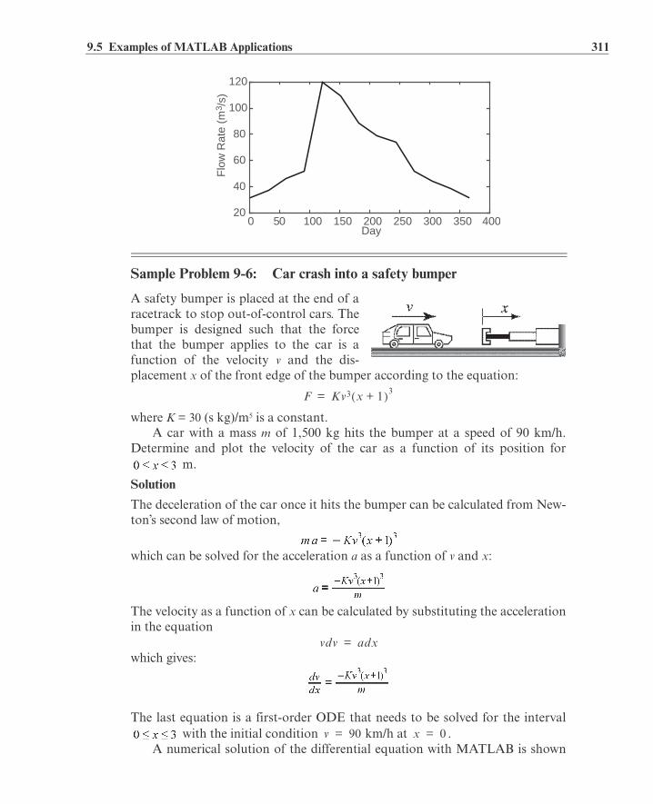
9.5 Examples of MATLAB Applications 311
Sample Problem 9-6: Car crash into a safety bumper
A safety bumper is placed at the end of aracetrack to stop out-of-control cars. Thebumper is designed such that the forcethat the bumper applies to the car is afunction of the velocity v and the dis-placement x of the front edge of the bumper according to the equation:
where K = 30 (s kg)/m5 is a constant.A car with a mass m of 1,500 kg hits the bumper at a speed of 90 km/h.
Determine and plot the velocity of the car as a function of its position for m.
Solution
The deceleration of the car once it hits the bumper can be calculated from New-ton’s second law of motion,
which can be solved for the acceleration a as a function of v and x:
The velocity as a function of x can be calculated by substituting the accelerationin the equation
which gives:
The last equation is a first-order ODE that needs to be solved for the interval with the initial condition km/h at .
A numerical solution of the differential equation with MATLAB is shown
Day0 50 100 150 200 250 300 350 400
Flo
w R
ate
(m3 /
s)20
40
60
80
100
120
F Kv3 x 1+ 3=
vdv adx=
v 90= x 0=

312 Chapter 9: Applications in Numerical Analysis
in the following program, which is written in a script file:
Note that the function handle @bumper is used for passing the user-definedfunction bumper into ode45. The listing of the user-defined function with thedifferential equation, named bumper, is:
When the script file executes (saved as Chap9SamPro6) the vectors x and v aredisplayed in the Command Window (actually, they are displayed on the screenone after the other, but to save room they are displayed below next to eachother).
global k m
k=30; m=1500; v0=90;
xspan=[0:0.2:3];
v0mps=v0*1000/3600;
[x v]=ode45(@bumper,xspan,v0mps)
plot(x,v)
xlabel('x (m)'); ylabel('velocity (m/s)')
function dvdx=bumper(x,v)
global k m
dvdx=-(k*v^2*(x+1)^3)/m;
>> Chap9SamPro6
x = 0
v = 25.0000
0.2000 22.0420
0.4000 18.4478
0.6000 14.7561
0.8000 11.4302
1.0000 8.6954
1.2000 6.5733
1.4000 4.9793
1.6000 3.7960
1.8000 2.9220
2.0000 2.2737
2.2000 1.7886
2.4000 1.4226
2.6000 1.1435
2.8000 0.9283
A vector that specifies the interval of the solution.
Changing the units of v0 to m/s.
Solving the ODE.

9.6 Problems 313
The plot generated by the program of the velocity as a function of distance is:
9.6 PROBLEMS
1. Determine the two solutions of the equation between and .
2. Determine the solution of the equation .
3. Determine the three roots of the equation .
4. Determine the positive roots of the equation .
5. The area A of a circle segment is given by:
Determine the angle (in degrees) if in. and
in2.
6. The position s of the slider as a func-tion of in the crank-slider mecha-nism shown is given by:
Given in., in., and in., determine the angle , when in. (There are two solutions.)
7. The van der Waals equation gives a relationship between the pressure p(atm), volume V (L), and temperature T (K) for a real gas:
3.0000 0.7607
x (m)0 0.5 1 1.5 2 2.5 3
velo
city
(m
/s)
0
5
10
15
20
25

314 Chapter 9: Applications in Numerical Analysis
where n is the number of moles, (L atm)/(mol K) is the gas con-
stant, and a (L2 atm/mol2) and b (L/mol) are material constants.
Determine the volume of 1.5 mol of nitrogen ( L2 atm/mol2, L/mol) at temperature of 350 K and pressure of 70 atm.
8. An estimate of the minimum velocity required for a round flat stone to skipwhen it hits the water is given by (Lyderic Bocquet, “The Physics of StoneSkipping,” Am. J. Phys., vol. 71, no. 2, February 2003):
where M and d are the stone mass and diameter, is the water density, C is
a coefficient, is the tilt angle of the stone, is the incidence angle, and
m/s2. Determine d if m/s. (Assume that kg,
, 1,000 kg/m3, and .)
9. A series RLC circuit with an AC voltagesource is shown. The amplitude of the cur-rent, I, in this circuit is given by:
where in which is the drivingfrequency; R and C are the resistance of theresistor and capacitance of the capacitor, respectively; and is the ampli-
tude of V. For the circuit in the figure , F,
H, and V.Determine for which A. (There are two solutions.)
10. For fluid flow in a pipe, the Colebrook–White (or Colebrook) equationgives a relationship between the friction coefficient, f, and the Reynoldsnumber:
where k/d is the pipe relative roughness. Determine f if , and
.
R 0.08206=
a 1.39=b 0.03913=
w
g 9.81= V 0.8= M 0.1=
C 1= w = 10= =
C
L
RV
d 2 fd= fd
vm
R 80=
vm 10=

9.6 Problems 315
11. Using MATLAB’s built-in function fminbnd, determine the minimum andthe maximum of the function
12. A flat rectangular sheet of metal that is70 in. wide and 120 in. long is formed tomake a container with the geometryshown in the figure. (Additional flatmetal pieces are attached at the ends.)Using MATLAB’s built-in functionfminbnd, determine the value of hsuch that the container will have themaximum possible volume, and deter-mine the corresponding volume.
13. Using MATLAB’s built-in function fminbnd,determine the dimensions (radius r and height h)and the volume of the cylinder with the largest vol-ume that can be made inside of a cone with aradius R of 20 in. and height H of 50 in.
14. A prismatic box with equilateral triangular base ismade from a equilateral triangular sheet with sides sby cutting off the corners and folding the edgesalong the dashed lines. For in., use MAT-LAB’s built-in function fminbnd to determine thevalue of x such that the box will have the maximumpossible volume, and determine the correspondingvolume.
15. An RLC circuit with an alternating voltagesource is shown. The source voltage isgiven by , where , inwhich is the driving frequency. The ampli-tude of the current, I, in this circuit is givenby:
where R and C are the resistance of the resistor and capacitance of the
capacitor, respectively. For the circuit in the figure F,
h
120 in.
4545
rh R=20 in.
H=50 in.
sx
C
L
R
vs
vs
vs vm dtsin= d 2 fd=
fd

316 Chapter 9: Applications in Numerical Analysis
H, , and V. Plot I as a function of f for Hz. Using MATLAB’s built-in function fminbnd, determine
the frequency where I is maximum and the corresponding value of I.
16. A 108-in.-long beam AB is attached tothe wall with a pin at point A and to a68-in.-long cable CD. A load lbis attached to the beam at point B. Thetension in the cable T is given by:
where L and LC are the lengths of the beam and the cable, respectively, and dis the distance from point A to point D, where the cable is attached. Make aplot of T versus d. Determine the distance d where the tension in the cable isthe smallest.
17. Use MATLAB to calculate the following integrals:
(a) (b)
18. Use MATLAB to calculate the following integrals:
(a) (b)
19. The speed of a race car during the first 7 s of a race is given by:
Determine the distance the car traveled during the first 7 s.
20. A rubber band is stretched by fixing one end pulling the other end. Mea-surements of the applied force at different displacements are given in the fol-lowing table:
Determine the work done by the force while stretching the rubber band.
t (s) 0 1 2 3 4 5 6 7v (mi/h) 0 14 39 69 95 114 129 139
x (in.) 0 0.4 0.8 1.2 1.6 2.0 2.4 2.8F (lb) 0 0.85 1.30 1.60 1.87 2.14 2.34 2.52
vm 26=
L
Wd
LC
A B
C
D
W 250=
1
11
2
7
0
3
0
8

9.6 Problems 317
21. Use numerical integration to approxi-mate the size of the shaded area shown inthe figure. Create a vector with values ofx from 1 through 10 and estimate the cor-responding y coordinate. Then, deter-mine the area by using MATLAB’s built-in function trapz.
22. The electric wire that connects the house to thepole has the shape of a catenary:
By using the equation:
determine the length of the wire.
23. The flow rate Q (volume of fluid per sec-ond) in a round pipe can be calculatedby:
For turbulent flow the velocity profile
can be estimated by: . Determine Q for in.,
, in./s.
24. The length of a curve given by a parametricequation , is given by:
The cardioid curve shown in the figure is givenby:
and with . Plot the cardioid with and determine the length of the curve.
25. The variation of gravitational acceleration g with altitude y is given by:
where km is the radius of the Earth, and m/s2 is thegravitational acceleration at sea level. The change in the gravitational poten-
1 2 3 4 5 6 7 8 9 10
1
2
3
4
5
6
x
y
x
y
-12 ft 26 ft
24 ft
L 1 f x 2+ xda
b=
rR
Q 2 vr rd0
r=
R 0.25=
n 7= vmax 80=
x
yx t y t
x t 2 y t 2+ tda
b
b 5=
gR2
R y+ 2---------------------g0=
R 6371= g0 9.81=
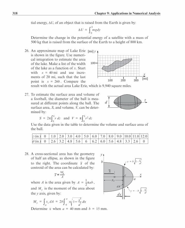
318 Chapter 9: Applications in Numerical Analysis
tial energy, U, of an object that is raised from the Earth is given by:
Determine the change in the potential energy of a satellite with a mass of500 kg that is raised from the surface of the Earth to a height of 800 km.
26. An approximate map of Lake Erieis shown in the figure. Use numeri-cal integration to estimate the areaof the lake. Make a list of the widthof the lake as a function of x. Startwith mi and use incre-ments of 20 mi, such that the lastpoint is . Compare theresult with the actual area Lake Erie, which is 9,940 square miles.
27. To estimate the surface area and volume ofa football, the diameter of the ball is mea-sured at different points along the ball. Thesurface area, S, and volume, V, can be deter-mined by:
and
Use the data given in the table to determine the volume and surface area ofthe ball.
28. A cross-sectional area has the geometryof half an ellipse, as shown in the figureto the right. The coordinate of thecentroid of the area can be calculated by:
where A is the area given by ,
and is the moment of the area aboutthe y axis, given by:
Determine when mm and mm.
z (in.) 0 1.0 2.0 3.0 4.0 5.0 6.0 7.0 8.0 9.0 10.0 11.0 12.0d (in.) 0 2.6 3.2 4.8 5.6 6 6.2 6.0 5.6 4.8 3.3 2.6 0
U mg yd0
h=
x
y
100 [mi]
[mi]
200 300
100
x 40=
x 260=
dz
S 2 r zd0
L= V r2 zd
0
L=
x
y
a
b
x
dx
xc
dA
c
y b 1x2
a2----–=
y b 1x2
a2-----––=
A12--- ab=
My
My xc AdA
2b0
a= =
a 40= b 15=

9.6 Problems 319
29. The orbit of Mercury is elliptical in shape, with
km and km. Theperimeter of an ellipse can be calculated by
where . Determine the distance Mer-
cury travels in one orbit. Calculate the average speed at which Mercury trav-els (in km/s) if one orbit takes about 88 days.
30. The Fresnel integrals are:
and
Calculate and for (use spacing of 0.05). In one figureplot two graphs—one of versus x and the other of versus x. In asecond figure plot versus .
31. Use a MATLAB built-in function to numerically solve:
for with
Plot the numerical solution.
32. Use a MATLAB built-in function to numerically solve:
for with
In one figure plot the numerical solution as a solid line and the exact solu-tion as discrete points.
Exact solution: .
33. Use a MATLAB built-in function to numerically solve:
for with
In one figure plot the numerical solution as a solid line and the exact solu-tion as discrete points (10 equally spaced points).
Exact solution: .
34. Use a MATLAB built-in function to numerically solve:
for with
Plot the solution.
ab
P 4a0
2
=
S x t 2sin td0
x= C x t 2cos td
0
x=
S x C x
S x C x
S x C x
y 0 2=
y 1 1=
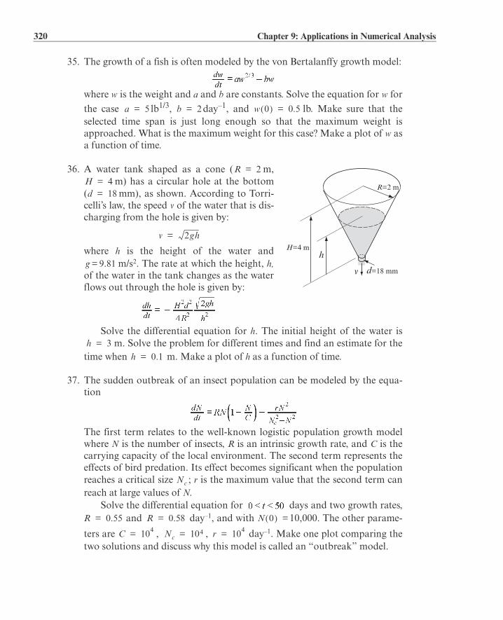
320 Chapter 9: Applications in Numerical Analysis
35. The growth of a fish is often modeled by the von Bertalanffy growth model:
where w is the weight and a and b are constants. Solve the equation for w for
the case lb1/3, day–1, and lb. Make sure that theselected time span is just long enough so that the maximum weight isapproached. What is the maximum weight for this case? Make a plot of w asa function of time.
36. A water tank shaped as a cone ( m,m) has a circular hole at the bottom
( mm), as shown. According to Torri-celli’s law, the speed v of the water that is dis-charging from the hole is given by:
where h is the height of the water andm/s2. The rate at which the height, h,
of the water in the tank changes as the waterflows out through the hole is given by:
Solve the differential equation for h. The initial height of the water ism. Solve the problem for different times and find an estimate for the
time when m. Make a plot of h as a function of time.
37. The sudden outbreak of an insect population can be modeled by the equa-tion
The first term relates to the well-known logistic population growth modelwhere N is the number of insects, R is an intrinsic growth rate, and C is thecarrying capacity of the local environment. The second term represents theeffects of bird predation. Its effect becomes significant when the populationreaches a critical size ; r is the maximum value that the second term canreach at large values of N.
Solve the differential equation for days and two growth rates, and day–1, and with 10,000. The other parame-
ters are , , day–1. Make one plot comparing thetwo solutions and discuss why this model is called an “outbreak” model.
a 5= b 2= w 0 0.5=
h
R=2 m
d=18 mm
H=4 m
v
R 2=H 4=d 18=
v 2gh=
g 9.81=
h 3=h 0.1=
Nc
R 0.55= R 0.58= N 0 =
C 104= Nc 104= r 104=

9.6 Problems 321
38. An airplane uses a parachuteand other means of braking as itslows down on the runway afterlanding. Its acceleration is given
by m/s2. Since
, the rate of change of the
velocity is given by:
Consider an airplane with a velocity of 300 km/h that opens its parachuteand starts decelerating at t = 0 s. (a) By solving the differential equation, determine and plot the velocity as a
function of time from t = 0 s until the airplane stops.(b) Use numerical integration to determine the distance x the airplane trav-
els as a function of time. Make a plot of x versus time.
39. The population growth of species with limited capacity can be modeled bythe equation:
where N is the population size, is the limiting number for the popula-
tion, and k, r, and are constants. The second term in the equation repre-sent the effect of predation. Consider the case where 6,000,
1/yr, 1/yr, 3,000, and . Determine N foryr. Make a plot of N as a function of t.
40. An RL circuit includes a voltagesource , a resistor , andan inductor H, as shown inthe figure. The differential equationthat describes the response of the cir-cuit is
where is the current in the inductor. Initially , and then at the voltage source is changed. Determine the response of the circuit for thefollowing three cases:
(a) V for .
(b) V for .
Nmax
Nc
Nmax =
k 0.196= r 40= Nc = N 0 50=
R
Lvs+_ vL (t)
vs R 1.8=
L 0.4=
LR----
diL
dt-------- iL+
vs
R----=
iL iL 0= t 0=
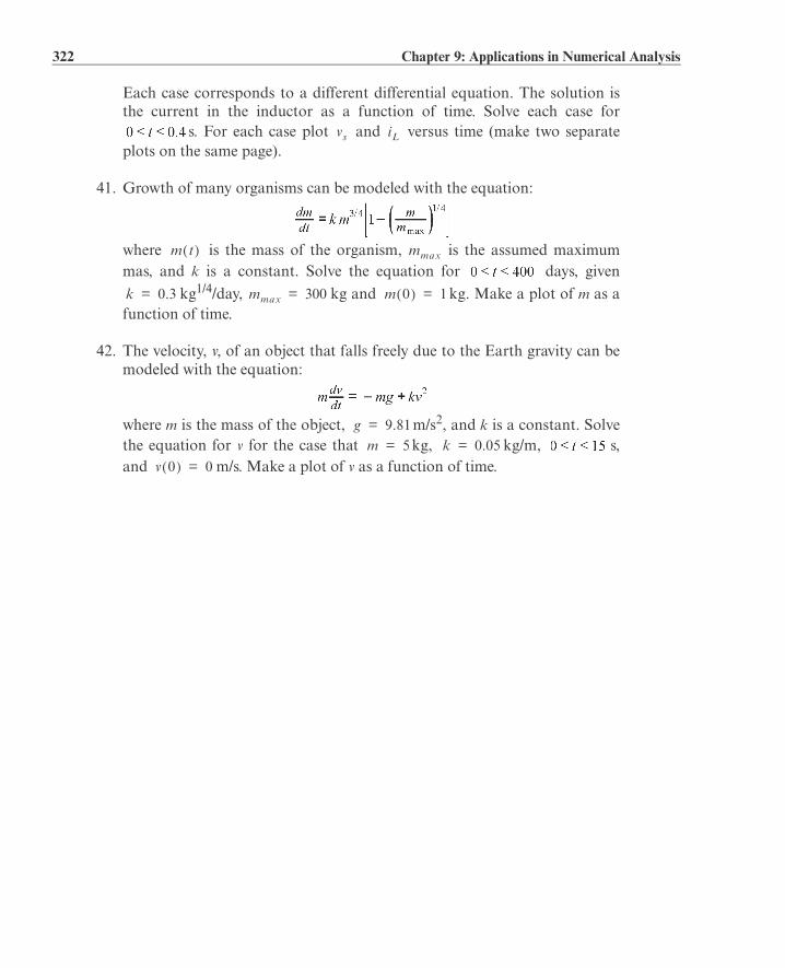
322 Chapter 9: Applications in Numerical Analysis
Each case corresponds to a different differential equation. The solution isthe current in the inductor as a function of time. Solve each case for
s. For each case plot and versus time (make two separateplots on the same page).
41. Growth of many organisms can be modeled with the equation:
where is the mass of the organism, is the assumed maximummas, and k is a constant. Solve the equation for days, given
kg1/4/day, kg and kg. Make a plot of m as afunction of time.
42. The velocity, v, of an object that falls freely due to the Earth gravity can bemodeled with the equation:
where m is the mass of the object, m/s2, and k is a constant. Solvethe equation for v for the case that kg, kg/m, s,and m/s. Make a plot of v as a function of time.
vs iL
m t mmax
k 0.3= mmax 300= m 0 1=
g 9.81=m 5= k 0.05=
v 0 0=

323
Chapter 10 Three-Dimensional Plots
Three-dimensional (3-D) plots can be a useful way to present data that consistsof more than two variables. MATLAB provides various options for displayingthree-dimensional data. They include line and wire, surface, mesh plots, andmany others. The plots can also be formatted to have a specific appearance andspecial effects. Many of the three-dimensional plotting features are described inthis chapter. Additional information can be found in the Help Window underPlotting and Data Visualization.
In many ways this chapter is a continuation of Chapter 5, where two-dimen-sional plots were introduced. The 3-D plots are presented in a separate chapterbecause not all MATLAB users use them. In addition, new users of MATLABwill probably find it easier to practice 2-D plotting first and learn the material inChapters 6–9 before attempting 3-D plotting. It is assumed throughout the restof this chapter that the reader is familiar with 2-D plotting.
10.1 LINE PLOTS
A three-dimensional line plot is a line that is obtained by connecting points inthree-dimensional space. A basic 3-D plot ‘is created with the plot3 command,which is very similar to the plot command and has the form:
• The three vectors with the coordinates of the data points must have the samenumber of elements.
plot3(x,y,z,‘line specifiers’,‘PropertyName’,property value)
(Optional) Specifiers thatdefine the type and colorof the line and markers.
x, y, and z arevectors of thecoordinates ofthe points.
(Optional) Properties with val-ues that can be used to specifythe line width, and marker’ssize and edge and fill colors.

324 Chapter 10: Three-Dimensional Plots
• The line specifiers, properties, and property values are the same as in 2-D plots(see Section 5.1).
For example, if the coordinates x, y, and z are given as a function of the parame-ter t by
a plot of the points for can be produced by the following script file:
The plot shown in Figure 10-1 is created when the script is executed.
10.2 MESH AND SURFACE PLOTS
Mesh and surface plots are three-dimensional plots used for plotting functionsof the form where x and y are the independent variables and z is thedependent variable. It means that within a given domain the value of z can becalculated for any combination of x and y. Mesh and surface plots are created inthree steps. The first step is to create a grid in the x y plane that covers thedomain of the function. The second step is to calculate the value of z at each
t=0:0.1:6*pi;
x=sqrt(t).*sin(2*t);
y=sqrt(t).*cos(2*t);
z=0.5*t;
plot3(x,y,z,'k','linewidth',1)
grid on
xlabel('x'); ylabel('y'); zlabel('z')
Figure 10-1: A plot of the function , , for .
x t 2tsin=
y t 2tcos=
z 0.5t=
5
x0
-5-5
0y
8
10
0
2
4
6
5
z
x t 2tsin= y t 2tcos= z 0.5t=
z f x y,=
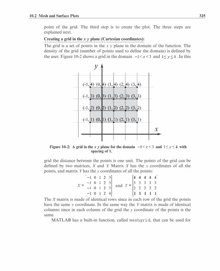
10.2 Mesh and Surface Plots 325
point of the grid. The third step is to create the plot. The three steps areexplained next.
Creating a grid in the x y plane (Cartesian coordinates):
The grid is a set of points in the x y plane in the domain of the function. Thedensity of the grid (number of points used to define the domain) is defined bythe user. Figure 10-2 shows a grid in the domain and . In this
grid the distance between the points is one unit. The points of the grid can bedefined by two matrices, X and Y. Matrix X has the x coordinates of all thepoints, and matrix Y has the y coordinates of all the points:
and
The X matrix is made of identical rows since in each row of the grid the pointshave the same x coordinate. In the same way the Y matrix is made of identicalcolumns since in each column of the grid the y coordinate of the points is thesame.
MATLAB has a built-in function, called meshgrid, that can be used for
Figure 10-2: A grid in the x y plane for the domain and with spacing of 1.
326 Chapter 10: Three-Dimensional Plots
creating the X and Y matrices. The form of the meshgrid function is:
In the vectors x and y the first and last elements are the respective boundaries ofthe domain. The density of the grid is determined by the number of elements inthe vectors. For example, the mesh matrices X and Y that correspond to the gridin Figure 10-2 can be created with the meshgrid command by:
Once the grid matrices exist, they can be used for calculating the value of z ateach grid point.
Calculating the value of z at each point of the grid:
The value of z at each point is calculated by using element-by-element calcula-tions in the same way it is used with vectors. When the independent variables xand y are matrices (they must be of the same size), the calculated dependentvariable is also a matrix of the same size. The value of z at each address is calcu-lated from the corresponding values of x and y. For example, if z is given by
the value of z at each point of the grid above is calculated by:
>> x=-1:3;
>> y=1:4;
>> [X,Y]=meshgrid(x,y)
X = -1 0 1 2 3 -1 0 1 2 3 -1 0 1 2 3 -1 0 1 2 3Y = 1 1 1 1 1 2 2 2 2 2 3 3 3 3 3 4 4 4 4 4
>> Z = X.*Y.^2./(X.^2 + Y.^2)
[X,Y] = meshgrid(x,y)
X is the matrix of the x coordi-nates of the grid points.Y is the matrix of the y coordi-nates of the grid points.
x is a vector that divides the domain of x.y is a vector that divides the domain of y.
zxy2
x2 y2+------------------=

10.2 Mesh and Surface Plots 327
Once the three matrices have been created, they can be used to plot mesh or sur-face plots.
Making mesh and surface plots:
A mesh or surface plot is created with the mesh or surf command, which hasthe form:
where X and Y are matrices with the coordinates of the grid and Z is a matrixwith the value of z at the grid points. The mesh plot is made of lines that connectthe points. In the surface plot, areas within the mesh lines are colored.
As an example, the following script file contains a complete program thatcreates the grid and then makes a mesh (or surface) plot of the function
over the domain and .
Note that in the program above the vectors x and y have a much smaller spacingthan the spacing earlier in the section. The smaller spacing creates a denser grid.The figures created by the program are:
Z = -0.5000 0 0.5000 0.4000 0.3000 -0.8000 0 0.8000 1.0000 0.9231 -0.9000 0 0.9000 1.3846 1.5000 -0.9412 0 0.9412 1.6000 1.9200
x=-1:0.1:3;
y=1:0.1:4;
[X,Y]=meshgrid(x,y);
Z=X.*Y.^2./(X.^2+Y.^2);
mesh(X,Y,Z)
xlabel('x'); ylabel('y'); zlabel('z')
mesh(X,Y,Z) surf(X,Y,Z)
zxy2
x2 y2+------------------=
Type surf(X,Y,Z) for surface plot.
42
x0-21
2y
3
-1
0
1
2
4
z
42
x0-21
2y3
2
1
0
-14
z
Surface plotMesh plot

328 Chapter 10: Three-Dimensional Plots
Additional comments on the mesh command:
• The plots that are created have colors that vary according to the magnitude of z.The variation in color adds to the three-dimensional visualization of the plots.The color can be changed to be a constant either by using the Plot Editor in theFigure Window (select the edit arrow, click on the figure to open the PropertyEditor Window, then change the color in the Mesh Properties list), or by usingthe colormap(C) command. In this command C is a three-element vector inwhich the first, second, and third elements specify the intensity of Red, Green,and Blue (RGB) colors, respectively. Each element can be a number between 0(minimum intensity) and 1 (maximum intensity). Some typical colors are:
C = [0 0 0] black C = [1 0 0] red C = [0 1 0] green C = [0 0 1] blue C = [1 1 0] yellow C = [1 0 1] magenta C = [0.5 0.5 0.5] gray
• When the mesh command executes, the grid is on by default. The grid can beturned off with the grid off command.
• A box can be drawn around the plot with the box on command.
• The mesh and surf commands can also be used with the form mesh(Z) andsurf(Z). In this case the values of Z are plotted as a function of theiraddresses in the matrix. The row number is on the x axis and the column numberis on the y axis.
There are several additional plotting commands that are similar to themesh and surf commands that create plots with different features. Table 10-1shows a summary of the mesh and surface plotting commands. All the examples
in the table are plots of the function over thedomain and .
Table 10-1: Mesh and surface plots
Plot type Example of plot Program
Mesh Plot
Function for-mat:mesh(X,Y,Z)
x=-3:0.25:3;y=-3:0.25:3;[X,Y] = meshgrid(x,y);Z=1.8.^(-1.5*sqrt(X.^2+ Y.̂ 2)).*cos(0.5*Y).*sin(X);mesh(X,Y,Z)xlabel('x'); ylabel('y') zlabel('z')
42
x0
-2-4-4
-20y
2
0.4
-0.2
0.2
0
-0.44
z

10.2 Mesh and Surface Plots 329
Surface Plot
Function for-mat:surf(X,Y,Z)
x=-3:0.25:3;y=-3:0.25:3;[X,Y] = meshgrid(x,y);Z=1.8.^(-1.5*sqrt(X.^2+Y.̂ 2)).*cos(0.5*Y).*sin(X);surf(X,Y,Z)xlabel('x'); ylabel('y')zlabel('z')
Mesh Curtain Plot (draws a curtain around the mesh)
Function for-mat:meshz(X,Y,Z)
x=-3:0.25:3;y=-3:0.25:3;[X,Y] = meshgrid(x,y);Z=1.8.^(-1.5*sqrt(X.^2+Y.̂ 2)).*cos(0.5*Y).*sin(X);meshz(X,Y,Z)xlabel('x'); ylabel('y')zlabel('z')
Mesh and Con-tour Plot (draws a contour plot beneath the mesh)
Function for-mat:meshc(X,Y,Z)
x=-3:0.25:3;y=-3:0.25:3;[X,Y] = meshgrid(x,y);Z=1.8.^(-1.5*sqrt(X.^2+Y.̂ 2)).*cos(0.5*Y).*sin(X);meshc(X,Y,Z)xlabel('x'); ylabel('y')zlabel('z')
Surface and Contour Plot (draws a contour plot beneath the surface)
Function for-mat:surfc(X,Y,Z)
x=-3:0.25:3;y=-3:0.25:3;[X,Y] = meshgrid(x,y);Z=1.8.^(-1.5*sqrt(X.^2+Y.̂ 2)).*cos(0.5*Y).*sin(X);surfc(X,Y,Z)xlabel('x'); ylabel('y')zlabel('z')
Table 10-1: Mesh and surface plots (Continued)
Plot type Example of plot Program
42
x0
-2-4-4
-20y
2
-0.2
0
0.2
0.4
-0.44
z
42
x0-2
-4-4-2
0y
2
0.4
0
0.2
-0.2
-0.44
z
42
0x-2
-4-4-2
y 02
-0.2
-0.4
0
0.4
0.2
4
z
42
x0
-2-4-4
-20y
2
-0.4
0.4
0.2
0
-0.2
4
z

330 Chapter 10: Three-Dimensional Plots
Surface Plot with Lighting
Function for-mat:surfl(X,Y,Z)
x=-3:0.25:3;y=-3:0.25:3;[X,Y] = meshgrid(x,y);Z=1.8.^(-1.5*sqrt(X.^2+Y.̂ 2)).*cos(0.5*Y).*sin(X);surfl(X,Y,Z)xlabel('x'); ylabel('y')zlabel('z')
Waterfall Plot (draws a mesh in one direction only)
Function for-mat:water-fall(X,Y,Z)
x=-3:0.25:3;y=-3:0.25:3;[X,Y] = meshgrid(x,y);[X,Y] = meshgrid(x,y);Z=1.8.^(-1.5*sqrt(X.^2+Y.̂ 2)).*cos(0.5*Y).*sin(X);waterfall(X,Y,Z)xlabel('x'); ylabel('y')zlabel('z')
3-D Contour Plot
Function for-mat:contour3(X, Y,Z,n)
n is the number of contour lev-els (optional)
x=-3:0.25:3;y=-3:0.25:3;[X,Y] = meshgrid(x,y);Z=1.8.^(-1.5*sqrt(X.^2+Y.̂ 2)).*cos(0.5*Y).*sin(X);contour3(X,Y,Z,15)xlabel('x'); ylabel('y')zlabel('z')
2-D Contour Plot(draws projec-tions of contour levels on the x y plane)Function format:contour (X,Y,Z,n)n is the number of contour lev-els (optional)
x=-3:0.25:3;y=-3:0.25:3;[X,Y ]=meshgrid(x,y);[X,Y] = meshgrid(x,y);Z=1.8.^(-1.5*sqrt(X.^2+Y.̂ 2)).*cos(0.5*Y).*sin(X);contour(X,Y,Z,15)xlabel('x'); ylabel('y')zlabel('z')
Table 10-1: Mesh and surface plots (Continued)
Plot type Example of plot Program
42
x0
-2-4-4
-20
y
2
-0.2
-0.4
0.4
0.2
0
4
z
42
x0-2
-4-4-2
0y
2
-0.2
0
0.2
0.4
-0.44
z
42
0x-2-4-4
-2y 02
0.4
0.2
0
-0.2
-0.44
z
x-3 -2 -1 0 1 2 3
y
-3
-2
-1
0
1
2
3

10.3 Plots with Special Graphics 331
10.3 PLOTS WITH SPECIAL GRAPHICS
MATLAB has additional functions for creating various types of special three-dimensional plots. A complete list can be found in the Help Window under Plot-ting and Data Visualization. Several of these 3-D plots are presented in Table10-2. The examples in the table do not show all the options available
Table 10-2: Specialized 3-D plots
Plot type Example of plot Program
Plot a Sphere
Function format:sphereReturns the x, y, and z coordi-nates of a unit sphere with 20 faces.sphere(n)Same as above with n faces.
sphere
or:
[X,Y,Z]=sphere(20);surf(X,Y,Z)
Plot a Cylinder
Function format:[X,Y,Z]=cylinder(r)Returns the x, y, and z coordi-nates of cylinder with profile r.
t=linspace(0,pi,20);r=1+sin(t);[X,Y,Z]=cylinder(r);surf(X,Y,Z)axis square
3-D Bar Plot
Function format:bar3(Y)Each element in Y is one bar. Col-umns are grouped together.
Y=[1 6.5 7; 2 6 7;3 5.5 7; 4 5 7; 3 47; 2 3 7; 1 2 7];bar3(Y)
1
0
-1-1
0
-1
1
0
1
2
0
-2-2
0
0.4
0.6
0.8
0
0.2
1
2
3217
65
43
21
8
6
4
2
0

332 Chapter 10: Three-Dimensional Plots
with each plot type. More details on each type of plot can be obtainedin the Help Window, or by typing help command_name in the Com-mand Window.Polar coordinates grid in the x y plane:
A 3-D plot of a function in which the value of z is given in polar coordinates (forexample ) can be done by following these steps:
• Create a grid of values of and r with the meshgrid function.
• Calculate the value of z at each point of the grid.
3-D Stem Plot (draws sequen-tial points with markers and ver-tical lines from the x y plane)
Function format:stem3(X,Y,Z)
t=0:0.2:10;x=t;y=sin(t);z=t.^1.5;stem3(x,y,z,'fill')grid onxlabel('x'); ylabel('y')zlabel('z')
3-D Scatter Plot
Function format:scatter3(X, Y,Z)
t=0:0.4:10;x=t;y=sin(t);z=t.^1.5;scatter3(x,y,z,'filled')grid oncolormap([0.1 0.1 0.1])xlabel('x');ylabel('y')zlabel('z')
3-D Pie Plot
Function format:pie3(X, explode)
X=[5 9 14 20];explode=[0 0 1 0];pie3(X,explode)
Table 10-2: Specialized 3-D plots (Continued)
Plot type Example of plot Program
10
x5
0-1
0y
30
40
0
10
20
1
z
10
5x
0-1
y 0
10
30
40
20
01
z
10%
19%
29%
42%
explode is a vector (same length as X) of 0’s and 1’s. 1 offsets the slice from the center.
z r=
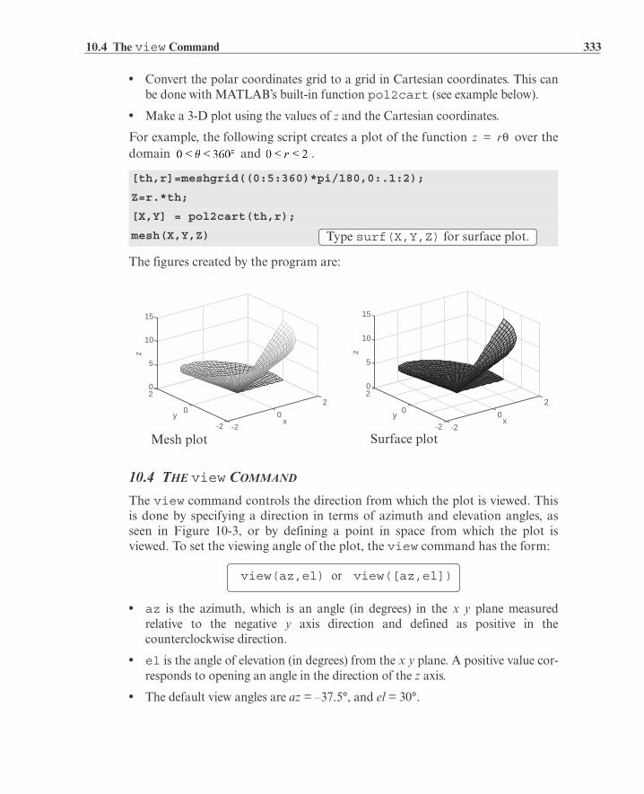
10.4 The view Command 333
• Convert the polar coordinates grid to a grid in Cartesian coordinates. This canbe done with MATLAB’s built-in function pol2cart (see example below).
• Make a 3-D plot using the values of z and the Cartesian coordinates.
For example, the following script creates a plot of the function over thedomain and .
The figures created by the program are:
10.4 THE view COMMAND
The view command controls the direction from which the plot is viewed. Thisis done by specifying a direction in terms of azimuth and elevation angles, asseen in Figure 10-3, or by defining a point in space from which the plot isviewed. To set the viewing angle of the plot, the view command has the form:
• az is the azimuth, which is an angle (in degrees) in the x y plane measuredrelative to the negative y axis direction and defined as positive in thecounterclockwise direction.
• el is the angle of elevation (in degrees) from the x y plane. A positive value cor-responds to opening an angle in the direction of the z axis.
• The default view angles are az = –37.5°, and el = 30°.
[th,r]=meshgrid((0:5:360)*pi/180,0:.1:2);
Z=r.*th;
[X,Y] = pol2cart(th,r);
mesh(X,Y,Z)
z r=
Type surf(X,Y,Z) for surface plot.
Mesh plot Surface plot
2
x0
-2-2
0y
0
5
10
15
2
z
2
x0
-2-2
0y
0
5
10
15
2
z
view(az,el) or view([az,el])

334 Chapter 10: Three-Dimensional Plots
As an example, the surface plot from Table 10-1 is plotted again in Figure 10-4,with viewing angles az = 20° and el = 35°.
• With the choice of appropriate azimuth and elevation angles, the view com-mand can be used to plot projections of 3-D plots on various planes accordingto the following table:
An example of a top view is shown next. Figure 10-5 shows the top view of thefunction that is plotted in Figure 10-1. Examples of projections onto the x z andy z planes are shown next, in Figures 10-6 and 10-7, respectively. The figuresshow mesh plot projections of the function plotted in Table 10-1.
Figure 10-3: Azimuth and elevation angles.
x=-3:0.25:3;y=-3:0.25:3;[X,Y]=meshgrid(x,y);Z=1.8.^(-1.5*sqrt(X.^2+Y.^2)).*cos(0.5*Y).*sin(X);surf(X,Y,Z)view(20,35)
Figure 10-4: A surface plot of the function with viewing angles of az = 20° and el = 35°.
Projection plane az value el value
x y (top view) 0 90
x z (side view) 0 0
y z (side view) 90 0
4
2
0 y-2
-442x
0-2
-4-0.4
0
-0.2
0.4
0.2
z

10.4 The view Command 335
t=0:0.1:6*pi;x=sqrt(t).*sin(2*t);y=sqrt(t).*cos(2*t);z=0.5*t;plot3(x,y,z,'k','linewidth',1)view(0,90)grid onxlabel('x'); ylabel('y') zlabel('z')
Figure 10-5: A top view plot of the function , , for .
x=-3:0.25:3;y=-3:0.25:3;[X,Y]=meshgrid(x,y);Z=1.8.^(-1.5*sqrt(X.^2+Y.^2)).*cos(0.5*Y).*sin(X);mesh(X,Y,Z)view(0,0)
Figure 10-6: Projections onto the x z plane of the function.
.
x=-3:0.25:3;y=-3:0.25:3;[X,Y]=meshgrid(x,y);Z=1.8.^(-1.5*sqrt(X.^2+Y.^2)).*cos(0.5*Y).*sin(X);surf(X,Y,Z)view(90,0)
Figure 10-7: Projections onto the y-z plane of the function.
.
-0.4
-0.3
-0.2
-0.1
0
0.1
0.2
0.3
0.4
x-3 -2 -1 0 1 2 3
x t 2tsin= y t 2tcos=z 0.5t=
z
-0.4
-0.3
-0.2
-0.1
0
0.1
0.2
0.3
0.4
x-3 -2 -1 0 1 2 3
z
-0.4
-0.3
-0.2
-0.1
0
0.1
0.2
0.3
0.4
y-3 -2 -1 0 1 2 3

336 Chapter 10: Three-Dimensional Plots
• The view command can also set a default view:
view(2) sets the default to the top view, which is a projection onto thex-y plane with az = 0°, and el = 90°.
view(3) sets the default to the standard 3-D view with az = –37.5° andel = 30°.
• The viewing direction can also be set by selecting a point in space from whichthe plot is viewed. In this case the view command has the formview([x,y,z]), where x, y, and z are the coordinates of the point. Thedirection is determined by the direction from the specified point to the origin ofthe coordinate system and is independent of the distance. This means that theview is the same with point [6, 6, 6] as with point [10, 10, 10]. Top view can be setup with [0, 0, 1]. A side view of the x z plane from the negative y direction can beset with [0, –1, 0], and so on.
10.5 EXAMPLES OF MATLAB APPLICATIONS
Sample Problem 10-1: 3-D projectile trajectory
A projectile is fired with an initial velocity of250 m/s at an angle of = 65° relative to theground. The projectile is aimed directlynorth. Because of a strong wind blowing tothe west, the projectile also moves in thisdirection at a constant speed of 30 m/s.Determine and plot the trajectory of the pro-jectile until it hits the ground. For compari-son, plot also (in the same figure) the trajectory that the projectile would havehad if there was no wind.
Solution
As shown in the figure, the coordinate system is set up such that the x and y axespoint in the east and north directions, respectively. Then the motion of the pro-jectile can be analyzed by considering the vertical direction z and the two hori-zontal components x and y. Since the projectile is fired directly north, the initialvelocity can be resolved into a horizontal y component and a vertical z com-ponent:
and
In addition, due to the wind the projectile has a constant velocity in the negativex direction, m/s.
The initial position of the projectile (x0, y0, z0) is at point (3000, 0, 0). In the ver-tical direction the velocity and position of the projectile are given by:
v0
v0y v0 cos= v0z v0 sin=

10.5 Examples of MATLAB Applications 337
and
The time it takes the projectile to reach the highest point is
. The total flying time is twice this time, . In the hori-
zontal direction the velocity is constant (both in the x and y directions), and theposition of the projectile is given by:
and
The following MATLAB program written in a script file solves the problem byfollowing the equations above.
The figure generated by the program is shown below.
v0=250; g=9.81; theta=65;
x0=3000; vx=-30;
v0z=v0*sin(theta*pi/180);
v0y=v0*cos(theta*pi/180);
t=2*v0z/g;
tplot=linspace(0,t,100);
z=v0z*tplot-0.5*g*tplot.^2;
y=v0y*tplot;
x=x0+vx*tplot;
xnowind(1:length(y))=x0;
plot3(x,y,z,'k-',xnowind,y,z,'k--')
grid on
axis([0 6000 0 6000 0 2700])
xlabel('x (m)'); ylabel('y (m)'); zlabel('z (m)')
vz 0=
thmax
v0z
g-------= ttot 2thmax=
x x0 vxt+= y y0 v0yt+=
Creating a time vector with 100 elements.
Calculating the x, y, and z coordi-nates of the projectile at each time.
Constant x coordinate when no wind.
Two 3-D line plots.
600050004000
x (m)30002000100000
2000
4000y (m)
2500
1500
1000
500
0
2000
6000
z (m
)

338 Chapter 10: Three-Dimensional Plots
Sample Problem 10-2: Electric potential of two point charges
The electric potential V around a charged particle is given by
where is the permittivity constant, q is the magni-
tude of the charge in coulombs, and r is the distance from the particle in meters.The electric field of two or more particles is calculated by using superposition.For example, the electric potential at a point due to two particles is given by
where , , , and are the charges of the particles and the distance fromthe point to the corresponding particle, respectively.
Two particles with a charge of
C and C are posi-tioned in the x y plane at points (0.25, 0, 0)and (–0.25, 0, 0), respectively, as shown.Calculate and plot the electric potential dueto the two particles at points in the x yplane that are located in the domain
and (the unitsin the x y plane are meters). Make the plotsuch that the x y plane is the plane of the points, and the z axis is the magnitudeof the electric potential.
Solution
The problem is solved by following these steps:(a) A grid is created in the x y plane with the domain and
.(b) The distance from each grid point to each of the charges is calculated.(c) The electric potential at each point is calculated. (d) The electric potential is plotted.The following is a program in a script file that solves the problem.
eps0=8.85e-12; q1=2e-10; q2=3e-10;
k=1/(4*pi*eps0);
x=-0.2:0.01:0.2;
y=-0.2:0.01:0.2;
[X,Y]=meshgrid(x,y);
r1=sqrt((X+0.25).^2+Y.^2);
V 14 0-------------q
r--=
0C
N m2---------------
V1
4 0-----------
q1
r1-----
q2
r2-----+=
q1 q2 r1 r2
Creating a grid in the x y plane.
Calculating the distance r1 for each grid point.

10.5 Examples of MATLAB Applications 339
The plot generated when the program runs is:
Sample Problem 10-3: Heat conduction in a square plate
Three sides of a rectangular plate (a = 5 m, b = 4m) are kept at a temperature of 0°C and one sideis kept at a temperature °C, as shown inthe figure. Determine and plot the temperaturedistribution T(x, y) in the plate.
Solution
The temperature distribution, T(x, y) in the plate can be determined by solvingthe two-dimensional heat equation. For the given boundary conditions T(x, y)can be expressed analytically by a Fourier series (Erwin Kreyszig, AdvancedEngineering Mathematics, John Wiley and Sons, 1993):
A program in a script file that solves the problem is listed below. The programfollows these steps:(a) Create an X, Y grid in the domain and . The length of the
plate, a, is divided into 20 segments, and the width of the plate, b, is dividedinto 16 segments.
(b) Calculate the temperature at each point of the mesh. The calculations are
r2=sqrt((X-0.25).^2+Y.^2);
V=k*(q1./r1+q2./r2);
mesh(X,Y,V)
xlabel('x (m)'); ylabel('y (m)'); zlabel('V (V)')
Calculating the distance r2 for each grid point.
Calculating the electric potential V at each grid point.
0.20.1
x (m)0
-0.1-0.2-0.2
-0.10
y (m)
0.1
10
20
30
60
40
50
0.2
V (
V)
T=0 a
b
x
y
T=0 T=0
T=80oCT1 80=
n 1=

340 Chapter 10: Three-Dimensional Plots
done point by point using a double loop. At each point the temperature isdetermined by adding k terms of the Fourier series.
(c) Make a surface plot of T.
The program was executed twice, first using five terms (k = 5) in the Fourierseries to calculate the temperature at each point, and then with k = 50. The meshplots created in each execution are shown in the figures below. The temperatureshould be uniformly 80°C at y = 4 m. Note the effect of the number of terms (k)on the accuracy at y = 4 m.
a=5; b=4; na=20; nb=16; k=5; T0=80;
clear T
x=linspace(0,a,na);
y=linspace(0,b,nb);
[X,Y]=meshgrid(x,y);
for i=1:nb
for j=1:na
T(i,j)=0;
for n=1:k
ns=2*n-1;
T(i,j)=T(i,j)+sin(ns*pi*X(i,j)/a).*sinh(ns*pi*Y(i,j)/a)/(sinh(ns*pi*b/a)*ns);
end
T(i,j) = T(i,j)*4*T0/pi;
end
end
mesh(X,Y,T)
xlabel('x (m)'); ylabel('y (m)'); zlabel('T ( ^oC)')
Creating a grid in the x y plane.
First loop, i, is the index of the grid’s row.
Second loop, j, is the index of the grid’s column.
Third loop, n, is the nth term of the Fourierseries, k is the number of terms.
54
x (m)3
21
001
2y (m)
3
80
60
40
20
100
04
T (
o C)
k = 50
54
x (m)3
21
001
2y (m)
3
100
80
60
40
20
04
T (
o C)
k = 5

10.6 Problems 341
10.6 PROBLEMS
1. The position of a moving particle as a function of time is given by:
Plot the position of the particle for s.
2. A staircase of height h is modeled by theparametric equations:
where , ,and m is the staircase height.Make a 3-D plot (shown) of the staircase.(Create a vector t for the domain 0 to ,and use the plot3 command.)
3. The ladder of a fire truck can be ele-vated (increase of angle ), rotatedabout the z axis (increase of angle ),and extended (increase of r). Initiallythe ladder rests on the truck ( ,
, and m). Then the ladderis moved to a new position by raisingthe ladder at a rate of 5 deg/s, rotatingat a rate of 8 deg/s, and extending theladder at a rate of 0.6 m/s. Determine and plot the position of the tip of theladder for 10 s.
4. Make a 3-D surface plot of the function in the domain
and .
5. Make a 3-D surface plot of the function in the domain and .
6. Make a 3-D surface plot of the function in the domain and .
7. Make a 3-D mesh plot of the function , where in
the domain and .
50
x (m)0
-50-50
0y (m)
40
60
0
20
50
z (m)
x r tcos= y r tsin= zht
2 n----------=
n 4=h 50=
2 n
0=0= r 8=
R x2 y2+=

342 Chapter 10: Three-Dimensional Plots
8. Make a 3-D surface plot of the function in the domain and .
9. Make a plot of the ice cream cone shown in the fig-ure. The cone is 8 in. tall with a 4-in. diameterbase. The ice cream at the top is a 4-in. diameterhemisphere.A parametric equation for the cone is:
, , with and
A parametric equation for a sphere is:, ,
with and
10. A monochromatic light that passes through aslit produces on a screen a diffraction patternconsisting of bright and dark fringes. Theintensity of the bright fringes, I, as a functionof can be calculated by:
where , is the light wave
length, a is the width of the slits. Makea 3-D plot (shown) that shows the rela-tive intensity as a function of
for , and a function of for .
11. Molecules of a gas in a container are moving around at different speeds.Maxwell’s speed distribution law gives the probability distribution as afunction of temperature and speed:
where M is the molar mass of the gas in kg/mol, J/(mol K), is thegas constant, T is the temperature in kelvins, and v is the molecule’s speed inm/s.
Make a 3-D plot of as a function of v and T for m/sand K for oxygen (molar mass 0.032 kg/mol).
−2
0
2
−2
0
20
2
4
6
8
10
z 4r=
x r sincos= y r sinsin= z rcos=
P v
R 8.31=
P v

10.6 Problems 343
12. Plank’s distribution law gives the black-body emissive power (amount of radiationenergy emitted) as a function of tempera-ture and wavelength:
where W m4/m2,
mK, T is the temperature in degrees K, and is the wave-length in m. Make a 3-D plot (shown in the figure) of as a function of
( m) and T for K. Use a logarithmic scale for. This can be done with the command: set(gca,'xscale','log').
13. Consider steady-state vibration of a fric-tion-free spring-mass-damper systemsubjected to harmonic applied force.The normalized amplitude of the massis given by:
where is the frequency ratio,and is the damping ratio. Make a 3-Dplot (shown) of the normalized ampli-tude (z axis) as a function of the fre-quency ratio for , and afunction of the damping ratio for
.
14. An RLC circuit with an alternatingvoltage source is shown. The sourcevoltage is given by
, where ,in which is the driving frequency.The amplitude of the current, I, inthis circuit is given by:
where R and C are the resistance of the resistor and capacitance of thecapacitor, respectively. For the circuit in the figure F,
H, and V.
(a) Make a 3-D plot of I (z axis) as a function of (x axis) for
Wm2 m----------------
E
21.5
Frequency Ratio
10.5
000.2
Damping Ratio
0.4
2
4
6
8
00.6N
orm
aliz
ed A
mpl
itude
vs
vs vm dtsin= d 2 fd=
fd
vm 24=
d

344 Chapter 10: Three-Dimensional Plots
Hz, and as a function of R (y axis) for ..
(b) Make a plot that is a projection on the x z plane. Estimate from this plotthe natural frequency of the circuit (the frequency at which I is maxi-
mum). Compare the estimate with the calculated value of .
15. In the solution of elasticity problem of a normal point load applied to thesurface of a half plane that was solved by Boussinesq in 1878, the stresses
and are given by:
and
where is Poisson’s ratio. For lb and, plot the stress components (each in a sep-
arate figure) as a function of r and z in thedomain and in. Plot thecoordinates r and z in the horizontal plane andthe stresses in the vertical direction.
16. A high-pass filter passes signals with frequenciesthat are higher than a certain cutoff frequency.In this filter the ratio of the magnitudes of thevoltages is given by:
where is the frequency of the input signal.
(a) Make a 3-D mesh plot of (z axis) as a function of f (x axis) for
Hz, and as a function of RC (y axis) for
s. Use a logarithmic scale for the x axis. Thiscan be done by typing the MATLAB commandset(gca,'Xscale','log') following the mesh command. A vec-tor with constant spacing on a logarithmic scale can be created with thecommand logspace(a,b,n).
(b) Make a plot that is a projection on the x z plane.
17. The equation for the streamlines for uniform flow over a cylinder is
where is the stream function. For example, if , then . Sincethe equation is satisfied for all x, the x axis is the zero ( ) streamline.
Observe that the collection of points where is also a streamline.Thus, the stream function above is for a cylinder of radius 1. Make a 2-D
Vi Vo
C
R
0=
0=
x2 y2+ 1=

10.6 Problems 345
contour plot of the streamlines around a cylinder with 1 in. radius. Set upthe domain for x and y to range between –3 and 3. Use 100 for the numberof contour levels. Add to the figure a plot of a circle with a radius of 1. Notethat MATLAB also plots streamlines inside the cylinder. This is a mathe-matical artifact.
18. The deflection w of a clamped circular membrane of radius subjected topressure P is given by (small deformation theory):
where r is the radial coordinate, and , where E, t, and are the
elastic modulus, thickness, and Poisson’s ratio of the membrane, respec-
tively. Consider a membrane with psi, in., psi,in., and . Make a surface plot of the membrane.
19. The Verhulst model, given in the following equation, describes the growth ofa population that is limited by various factors such as overcrowding andlack of resources:
where is the number of individuals in the population, is the initialpopulation size, is the maximum population size possible due to the var-ious limiting factors, and r is a rate constant. Make a surface plot of versus t and assuming s–1, and . Let t vary between 0and 100 and between 100 and 1,000.
20. The geometry of a ship hull (Wigleyhull) can be modeled by the equa-tion:
where x, y, and z are the length,width, and height, respectively. UseMATLAB to make a 3-D figure ofthe hull as shown. Use ,
, , , and .
rd
P 15= rd 15=
t 0.08=
N t N0
N
N t
N r 0.1= N0 10=N
−20
2
−1
0
1
−0.4
−0.2
0
xy
z
B 1.2=L 4= T 0.5=

346 Chapter 10: Three-Dimensional Plots
21. The stress fields near a crack tip of alinear elastic isotropic material formode II loading are given by:
For ksi plot the stresses (each in a separate figure) in thedomain and in. Plot the coordinates x and y in thehorizontal plane, and the stresses in the vertical direction.
22. A ball thrown up falls back to the floorand bounces many times. For a ballthrown up in the direction shown in thefigure, the position of the ball as a func-tion of time is given by:
The velocities in the x and y directions areconstants throughout the motion and aregiven by and
. In the vertical z
direction the initial velocity is, and when the ball impacts
the floor its rebound velocity is 0.8 of thevertical velocity at the start of the previousbounce. The time between bounces isgiven by , where is the verti-cal component of the velocity at the startof the bounce. Make a 3-D plot (shown inthe figure) that shows the trajectory of theball during the first five bounces. Take m/s, , , and
m/s2.
KII 300=
050
100
050
100150
0
5
10
x (m)y (m)
z (m
)
x vxt= y vyt=
vx v0 cossin=
vy v0 sinsin=
vz v0 cos=
vz
v0 20= 30= 25=
g 9.81=

347
Chapter 11 Symbolic Math
All of the mathematical operations done with MATLAB in the first 10 chapterswere numerical. The operations were carried out by writing numerical expres-sions that could contain numbers and variables with preassigned numerical val-ues. When a numerical expression is executed by MATLAB, the outcome is alsonumerical (a single number or an array with numbers). The number, or num-bers, are either exact or a floating point–approximated value. For example, typ-ing 1/4 gives 0.2500—an exact value, and typing 1/3 gives 0.3333—anapproximated value.
Many applications in math, science, and engineering require symbolic oper-ations, which are mathematical operations with expressions that contain sym-bolic variables (variables that don’t have specific numerical values when theoperation is executed). The result of such operations is also a mathematicalexpression in terms of the symbolic variables. One simple example involves solv-ing an algebraic equation that contains several variables and solving for onevariable in terms of the others. If a, b, and x are symbolic variables, and
, x can be solved in terms of a and b to give . Other examplesof symbolic operations are analytical differentiation or integration of mathe-
matical expressions. For instance, the derivative of with respect to tis .
MATLAB has the capability of carrying out many types of symbolic opera-tions. The numerical part of the symbolic operation is carried out by MATLABexactly, with no approximation of numerical values. For example, the result of
adding and is and not 0.5833x.
Symbolic operations can be performed by MATLAB once the SymbolicMath Toolbox is installed. The Symbolic Math Toolbox is a collection of MAT-LAB functions that are used for execution of symbolic operations. The com-mands and functions for the symbolic operations have the same style and syntaxas those for the numerical operations. The symbolic operations themselves areexecuted primarily by MuPad®, which is mathematical software designed forthis purpose. The MuPad software is embedded within MATLAB and is auto-matically activated when a symbolic MATLAB function is executed. MuPad
6t2 5+
348 Chapter 11: Symbolic Math
can also be used as separate independent software. That software uses theMuPAD language, which has a completely different structure and commandsthan MATLAB. The Symbolic Math Toolbox is included in the student versionof MATLAB. In the standard version, the toolbox is purchased separately. Tocheck if the Symbolic Math Toolbox is installed on a computer, the user cantype the command ver in the Command Window. In response, MATLAB dis-plays information about the version that is used as well as a list of the toolboxesthat are installed.
The starting point for symbolic operations is symbolic objects. Symbolicobjects are made of variables and numbers that, when used in mathematicalexpressions, tell MATLAB to execute the expression symbolically. Typically, theuser first defines (creates) the symbolic variables (objects) that are needed, andthen uses them to create symbolic expressions that are subsequently used insymbolic operations. If needed, symbolic expressions can be used in numericaloperations
The first section in this chapter describes how to define symbolic objectsand how to use them to create symbolic expressions. The second section showshow to change the form of existing expressions. Once a symbolic expression hasbeen created, it can be used in mathematical operations. MATLAB has a largeselection of functions for this purpose. The next four sections (11.3–11.6)describe how to use MATLAB to solve algebraic equations, to carry out differ-entiation and integration, and to solve differential equations. Section 11.7 cov-ers plotting symbolic expressions. How to use symbolic expressions insubsequent numerical calculations is explained in the following section.
11.1 SYMBOLIC OBJECTS AND SYMBOLIC EXPRESSIONS
A symbolic object can be a variable (without a preassigned numerical value), anumber, or an expression made of symbolic variables and numbers. A symbolicexpression is a mathematical expression containing one or more symbolicobjects. When typed, a symbolic expression may look like a standard numericalexpression. However, because the expression contains symbolic objects, it is exe-cuted by MATLAB symbolically.
11.1.1 Creating Symbolic Objects
Symbolic objects can be variables or numbers. They can be created with the symand/or syms commands. A single symbolic object can be created with the symcommand:
where the string, which is the symbolic object, is assigned to a name. The stringcan be:• A single letter or a combination of several letters (no spaces). Examples: ‘a’,
‘x’, ‘yad’.
object_name = sym(‘string’)
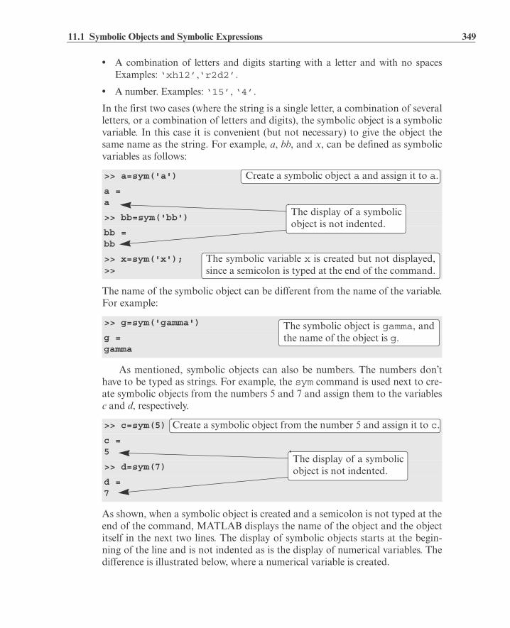
11.1 Symbolic Objects and Symbolic Expressions 349
• A combination of letters and digits starting with a letter and with no spacesExamples: ‘xh12’,‘r2d2’.
• A number. Examples: ‘15’, ‘4’.
In the first two cases (where the string is a single letter, a combination of severalletters, or a combination of letters and digits), the symbolic object is a symbolicvariable. In this case it is convenient (but not necessary) to give the object thesame name as the string. For example, a, bb, and x, can be defined as symbolicvariables as follows:
The name of the symbolic object can be different from the name of the variable.For example:
As mentioned, symbolic objects can also be numbers. The numbers don’thave to be typed as strings. For example, the sym command is used next to cre-ate symbolic objects from the numbers 5 and 7 and assign them to the variablesc and d, respectively.
As shown, when a symbolic object is created and a semicolon is not typed at theend of the command, MATLAB displays the name of the object and the objectitself in the next two lines. The display of symbolic objects starts at the begin-ning of the line and is not indented as is the display of numerical variables. Thedifference is illustrated below, where a numerical variable is created.
>> a=sym('a')
a =a
>> bb=sym('bb')
bb =bb
>> x=sym('x');>>
>> g=sym('gamma')
g =gamma
>> c=sym(5)
c =5
>> d=sym(7)
d =7
Create a symbolic object a and assign it to a.
The display of a symbolicobject is not indented.
The symbolic variable x is created but not displayed,since a semicolon is typed at the end of the command.
The symbolic object is gamma, andthe name of the object is g.
Create a symbolic object from the number 5 and assign it to c.
The display of a symbolicobject is not indented.

350 Chapter 11: Symbolic Math
Several symbolic variables can be created in one command by using thesyms command, which has the form:
The command creates symbolic objects that have the same names as the sym-bolic variables. For example, the variables y, z, and d can all be created as sym-bolic variables in one command by typing:
When the syms command is executed, the variables it creates are not displayedautomatically—even if a semicolon is not typed at the end of the command.
11.1.2 Creating Symbolic Expressions
Symbolic expressions are mathematical expressions written in terms of symbolicvariables. Once symbolic variables are created, they can be used for creatingsymbolic expressions. The symbolic expression is a symbolic object (the displayis not indented). The form for creating a symbolic expression is:
A few examples are:
When a symbolic expression, which includes mathematical operations that canbe executed (addition, subtraction, multiplication, and division), is entered,MATLAB executes the operations as the expression is created. For example:
>> e=13
e = 13
>> syms y z d
>> yy =y
>> syms a b c x y
>> f=a*x^2+b*x + c
f =a*x^2 + b*x + c
>> g=2*a/3+4*a/7-6.5*x+x/3+4*5/3-1.5
The display of the value of anumerical variable is indented.
13 is assigned to e (numerical variable).
syms variable_name variable_name variable_name
The variables created by the syms command arenot displayed automatically. Typing the name ofthe variable shows that the variable was created.
Expression_name = Mathematical expression
Define a, b, c, x, and y as symbolic variables.
Create the symbolic expression and assign it to f.ax2 bx c+ +
The display of the symbolic expression is not indented.
is entered.

11.1 Symbolic Objects and Symbolic Expressions 351
Notice that all the calculations are carried out exactly, with no numerical
approximation. In the last example, and were added by MATLAB to
give , and was added to . The operations with the terms
that contain only numbers in the symbolic expression are carried out exactly. In
the last example, is replaced by .
The difference between exact and approximate calculations is demonstratedin the following example, where the same mathematical operations are carriedout—once with symbolic variables and once with numerical variables.
An expression that is created can include both symbolic objects and numer-ical variables. However, if an expression includes a symbolic object (or several),all the mathematical operations will be carried out exactly. For example, if c isreplaced by a in the last expression, the result is exact, as it was in the first exam-ple.
Additional facts about symbolic expressions and symbolic objects:
• Symbolic expressions can include numerical variables that have been obtainedfrom the execution of numerical expressions. When these variables are insertedin symbolic expressions their exact value is used, even if the variable was dis-played before with an approximated value. For example:
g =(26*a)/21 - (37*x)/6 + 31/6
>> a=sym(3); b=sym(5);
>> e=b/a+sqrt(2)
e =2^(1/2) + 5/3
>> c=3; d=5;
>> f=d/c+sqrt(2)
f = 3.0809
>> g=d/a+sqrt(2)
g =2^(1/2) + 5/3
>> h=10/3
h = 3.3333
is displayed.
Define a and b as symbolic 3 and 5, respectively.
Create an expression that includes a and b.
An exact value of e is displayed as a sym-bolic object (the display is not indented).
Define c and d as numerical 3 and 5, respectively.
Create an expression that includes c and d.
An approximated value of f is displayedas a number (the display is indented).
h is defined to be 10/3 (a numerical variable).
An approximated value of h (numerical variable) is displayed.
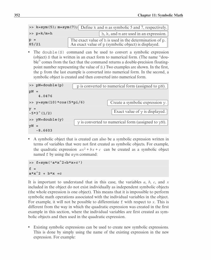
352 Chapter 11: Symbolic Math
• The double(S) command can be used to convert a symbolic expression(object) S that is written in an exact form to numerical form. (The name “dou-ble” comes from the fact that the command returns a double-precision floating-point number representing the value of S.) Two examples are shown. In the first,the p from the last example is converted into numerical form. In the second, asymbolic object is created and then converted into numerical form.
• A symbolic object that is created can also be a symbolic expression written interms of variables that were not first created as symbolic objects. For example,the quadratic expression can be created as a symbolic objectnamed f by using the sym command:
It is important to understand that in this case, the variables a, b, c, and xincluded in the object do not exist individually as independent symbolic objects(the whole expression is one object). This means that it is impossible to performsymbolic math operations associated with the individual variables in the object.For example, it will not be possible to differentiate f with respect to x. This isdifferent from the way in which the quadratic expression was created in the firstexample in this section, where the individual variables are first created as sym-bolic objects and then used in the quadratic expression.
• Existing symbolic expressions can be used to create new symbolic expressions.This is done by simply using the name of the existing expression in the newexpression. For example:
>> k=sym(5); m=sym(7);
>> p=k/m+h
p =85/21
>> pN=double(p)
pN = 4.0476
>> y=sym(10)*cos(5*pi/6)
y =-5*3^(1/2)
>> yN=double(y)
yN = -8.6603
>> f=sym('a*x^2+b*x+c')
f =a*x^2 + b*x +c
Define k and m as symbolic 5 and 7, respectively.
h, k, and m are used in an expression.
The exact value of h is used in the determination of p.An exact value of p (symbolic object) is displayed.
p is converted to numerical form (assigned to pN).
Create a symbolic expression y.
Exact value of y is displayed.
y is converted to numerical form (assigned to yN).
ax2 bx c+ +

11.1 Symbolic Objects and Symbolic Expressions 353
11.1.3 The findsym Command and the Default Symbolic Variable
The findsym command can be used to find which symbolic variables are pres-ent in an existing symbolic expression. The format of the command is:
The findsym(S) command displays the names of all the symbolic variables(separated by commas) that are in the expression S in alphabetical order. Thefindsym(S,n) command displays n symbolic variables that are in expressionS in the default order. For one-letter symbolic variables, the default order startswith x, and followed by letters, according to their closeness to x. If there are twoletters equally close to x, the letter that is after x in alphabetical order is first (ybefore w, and z before v). The default symbolic variable in a symbolic expressionis the first variable in the default order. The default symbolic variable in anexpression S can be identified by typing findsym(S,1). Examples:
>> syms x y
>> SA=x+y, SB=x-y
SA =x+ySB =x-y
>> F=SA^2/SB^3+x^2
F =(x+y)^2/(x-y)^3+x^2
>> syms x h w y d t
>> S=h*x^2+d*y^2+t*w^2
S =t*w^2 + h*x^2 + d*y^2
>> findsym(S)
ans =d, h, t, w, x, y
>> findsym(S,5)
ans =x,y,w,t,h
>> findsym(S,1)
ans =x
Define x and y as symbolic variables.
Create two symbolic expressions SA and SB.
SA x y+=
Create a new symbolic expression F using SA and SB.
findsym(S) findsym(S,n)or
Define x, h, w, y, d, and t as symbolic variables.
Create a symbolic expression S.
Use the findsym(S) command.
The symbolic variables are displayed in alphabetical order.
Use the findsym(S,n) command (n = 5).
Five symbolic variables are displayed in the default order.
Use the findsym(S,n) command with n = 1.
The default symbolic variable is displayed.

354 Chapter 11: Symbolic Math
11.2 CHANGING THE FORM OF AN EXISTING SYMBOLIC EXPRESSION
Symbolic expressions are either created by the user or by MATLAB as the resultof symbolic operations. The expressions created by MATLAB might not be inthe simplest form or in a form that the user prefers. The form of an existing sym-bolic expression can be changed by collecting terms with the same power, byexpanding products, by factoring out common multipliers, by using mathemati-cal and trigonometric identities, and by many other operations. The followingsubsections describe several of the commands that can be used to change theform of an existing symbolic expression.
11.2.1 The collect, expand, and factor Commands
The collect, expand, and factor commands can be used to perform themathematical operations that are implied by their names.
The collect command:
The collect command collects the terms in the expression that have the vari-able with the same power. In the new expression, the terms will be ordered indecreasing order of power. The command has the forms
where S is the expression. The collect(S) form works best when an expres-sion has only one symbolic variable. If an expression has more than one vari-able, MATLAB will collect the terms of one variable first, then those of asecond variable, and so on. The order of the variables is determined by MAT-LAB. The user can specify the first variable by using the collect(S, vari-
able_name) form of the command. Examples:
>> syms x y
>> S=(x^2+x-exp(x))*(x+3)S =(x + 3)*(x - exp(x) + x^2)
>> F = collect(S)
F =x^3+4*x^2+(3-exp(x))*x-3*exp(x)
>> T=(2*x^2+y^2)*(x+y^2+3)T =(2*x^2+y^2)*(y^2+x+3)
>> G=collect(T)
collect(S) collect(S, variable_name)
Define x and y as symbolic variables.
Create the symbolic expression
and assign it to S.
Use the collect command.
MATLAB returns the expression:.
Create the symbolic expression T .2x2 y2+ y2 x 3+ +
Use the collect(T) command.
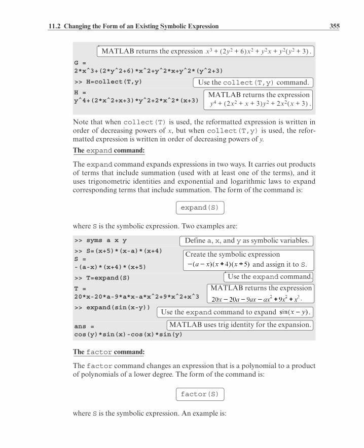
11.2 Changing the Form of an Existing Symbolic Expression 355
Note that when collect(T) is used, the reformatted expression is written inorder of decreasing powers of x, but when collect(T,y) is used, the refor-matted expression is written in order of decreasing powers of y.
The expand command:
The expand command expands expressions in two ways. It carries out productsof terms that include summation (used with at least one of the terms), and ituses trigonometric identities and exponential and logarithmic laws to expandcorresponding terms that include summation. The form of the command is:
where S is the symbolic expression. Two examples are:
The factor command:
The factor command changes an expression that is a polynomial to a productof polynomials of a lower degree. The form of the command is:
where S is the symbolic expression. An example is:
G =2*x^3+(2*y^2+6)*x^2+y^2*x+y^2*(y^2+3)
>> H=collect(T,y)
H =y^4+(2*x^2+x+3)*y^2+2*x^2*(x+3)
>> syms a x y
>> S=(x+5)*(x-a)*(x+4)S =-(a-x)*(x+4)*(x+5)
>> T=expand(S)
T =20*x-20*a-9*a*x-a*x^2+9*x^2+x^3
>> expand(sin(x-y))
ans =cos(y)*sin(x)-cos(x)*sin(y)
MATLAB returns the expression .2x3 2y2 6+ x2 y2x y2 y2 3++ + +
Use the collect(T,y) command.
MATLAB returns the expression.y4 2x2 x 3+ + y2 2x2 x 3++ +
expand(S)
Define a, x, and y as symbolic variables.
Create the symbolic expression and assign it to S.
Use the expand command.
MATLAB returns the expression.
Use the expand command to expand .
MATLAB uses trig identity for the expansion.
factor(S)

356 Chapter 11: Symbolic Math
11.2.2 The simplify Command
The simplify command is a tool for simplifying the form of an expression.The simplify command uses mathematical operations (addition, multiplica-tion, rules of fractions, powers, logarithms, etc.) and functional and trigonomet-ric identities to generate a simpler form of the expression. The format of thesimplify command is:
Two examples are:
11.2.3 The pretty Command
The pretty command displays a symbolic expression in a format resemblingthe mathematical format in which expressions are generally typed. The com-mand has the form
Example:
>> syms x
>> S=x^3+4*x^2-11*x-30S =x^3+4*x^2-11*x-30
>> factor(S)
ans =(x+5)*(x-3)*(x+2)
>> syms x y
>> S=(x^2+5*x+6)/(x+2)
S =(x^2+5*x+6)/(x+2)
>> SA = simplify(S)
SA =x+3
>> simplify((x+y)/(1/x+1/y))
ans =x*y
Define x as a symbolic variable.
Create the symbolic expression and assign it to S.
Use the factor command.
MATLAB returns the expression.
simplify(S)
where either S is the name of the existing expression to be simplified,
an expression to be simplified can be typed in for S.
or
Define x and y as symbolic variables.
Create the symbolic expression
, and assign it to S.
Use the simplify command to simplify S.
MATLAB simplifies the expres-sion to .x 3+
Simplify .
MATLAB simplifies the expression to ).xy
pretty(S)
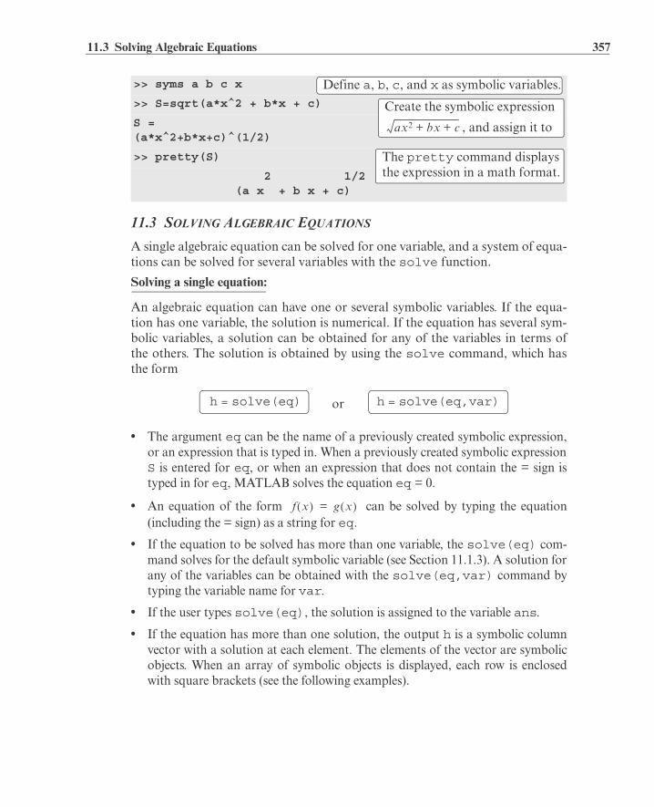
11.3 Solving Algebraic Equations 357
11.3 SOLVING ALGEBRAIC EQUATIONS
A single algebraic equation can be solved for one variable, and a system of equa-tions can be solved for several variables with the solve function.
Solving a single equation:
An algebraic equation can have one or several symbolic variables. If the equa-tion has one variable, the solution is numerical. If the equation has several sym-bolic variables, a solution can be obtained for any of the variables in terms ofthe others. The solution is obtained by using the solve command, which hasthe form
• The argument eq can be the name of a previously created symbolic expression,or an expression that is typed in. When a previously created symbolic expressionS is entered for eq, or when an expression that does not contain the = sign istyped in for eq, MATLAB solves the equation eq = 0.
• An equation of the form can be solved by typing the equation(including the = sign) as a string for eq.
• If the equation to be solved has more than one variable, the solve(eq) com-mand solves for the default symbolic variable (see Section 11.1.3). A solution forany of the variables can be obtained with the solve(eq,var) command bytyping the variable name for var.
• If the user types solve(eq), the solution is assigned to the variable ans.
• If the equation has more than one solution, the output h is a symbolic columnvector with a solution at each element. The elements of the vector are symbolicobjects. When an array of symbolic objects is displayed, each row is enclosedwith square brackets (see the following examples).
>> syms a b c x
>> S=sqrt(a*x^2 + b*x + c)
S =(a*x^2+b*x+c)^(1/2)
>> pretty(S)
2 1/2 (a x + b x + c)
Define a, b, c, and x as symbolic variables.
Create the symbolic expression
, and assign it to ax2 bx c+ +
The pretty command displays the expression in a math format.
h = solve(eq) h = solve(eq,var)or
f x g x=

358 Chapter 11: Symbolic Math
The following examples illustrate the use of the solve command.
• It is also possible to use the solve command by typing the equation to besolved as a string, without having the variables in the equation first created assymbolic objects. However, if the solution contains variables (when the equationhas more than one variable), the variables do not exist as independent symbolicobjects. For example:
>> syms a b x y z
>> h=solve(exp(2*z)-5)
h =log(5)/2
>> S=x^2-x-6S =x^2-x-6
>> k=solve(S)
k = -2 3
>> solve('cos(2*y)+3*sin(y)=2')
ans = pi/2 pi/6 (5*pi)/6
>> T= a*x^2+5*b*x+20T =a*x^2+5*b*x+20
>> solve(T)
ans = -(5*b+5^(1/2)*(5*b^2-16*a)^(1/2))/(2*a) -(5*b-5^(1/2)*(5*b^2-16*a)^(1/2))/(2*a)
>> M = solve(T,a)
M =-(5*b*x+20)/x^2
>> ts=solve('4*t*h^2+20*t-5*g')
ts =(5*g)/(4*h^2+20)
Define a, b, x, y, and z as symbolic variables.
Use the solve command to solve .
The solution is assigned to h.
Create the symbolic expression , and assign it to S.
Use the solve(S)command to solve .
The equation has two solutions. They are assigned to k, which is a column vector with symbolic
Use the solve command to solve . (The equation is typed as a string in the command.)
2ycos 3 ysin+ 2=
The solution is assigned to ans.
Create the symbolic expression , and assign it to T.ax2 5bx 20+ +
Use the solve(S)command to solve .T 0=
The equation is solved for the vari-able x, which is the default variable.
T 0=
Use the solve(eq,var)command to solve .T 0=
The equation is solved for the variable a.T 0=
The expression is typed in
the solve command.
The variables t, h, and g were not created as symbolic variables before the expression was typed in the solve command.
MATLAB solves the equation for t.

11.3 Solving Algebraic Equations 359
The equation can also be solved for a different variable. For example, a solu-tion for g is obtained by:
Solving a system of equations:
The solve command can also be used for solving a system of equations. If thenumber of equations and the number of variables are the same, the solution isnumerical. If the number of variables is greater than the number of equations,the solution is symbolic for the desired variables in terms of the other variables.A system of equations (depending on the type of equations) can have one or sev-eral solutions. If the system has one solution, each of the variables for which thesystem is solved has one numerical value (or expression). If the system has morethan one solution, each of the variables can have several values.
The format of the solve command for solving a system of n equations is:
• The arguments eq1,eq2,...,eqn are the equations to be solved. Each argu-ment can be a name of a previously created symbolic expression, or an expres-sion that is typed in as a string. When a previously created symbolic expressionS is entered, the equation is S = 0. When a string that does not contain the =sign is typed in, the equation is expression = 0. An equation that containsthe = sign must be typed as a string.
• In the first format, if the number of equations n is equal to the number of vari-ables in the equations, MATLAB gives a numerical solution for all the variables.If the number of variables is greater than the number of equations n, MATLABgives a solution for n variables in terms of the rest of the variables. The variablesfor which solutions are obtained are chosen by MATLAB according to thedefault order (Section 11.1.3).
• When the number of variables is greater than the number of equations n, theuser can select the variables for which the system is solved. This is done by usingthe second format of the solve command and entering the names of the vari-ables var1,var2,...,varn.
The output from the solve command, which is the solution of the sys-tem, can have two different forms. One is a cell array and the other is a structure.A cell array is an array in which each of the elements can be an array. A struc-
>> gs=solve('4*t*h^2+20*t-5*g','g')
gs =(4*t*h^2)/5 + 4*t
output = solve(eq1,eq2,....,eqn)
output = solve(eq1,eq2,...,eqn,var1,var2,...,varn)
or

360 Chapter 11: Symbolic Math
ture is an array in which the elements (called fields) are addressed by textualfield designators. The fields of a structure can be arrays of different sizes andtypes. Cell arrays and structures are not presented in detail in this book, but ashort explanation is given below so that the reader will be able to use them withthe solve command.
When a cell array is used in the output of the solve command, the com-mand has the following form (in the case of a system of three equations):
[varA, varB, varC] = solve(eq1,eq2,eq3)
• Once the command is executed, the solution is assigned to the variables varA,varB, and varC, and the variables are displayed with their assigned solution.Each of the variables will have one or several values (in a column vector)depending on whether the system of equations has one or several solutions.
• The user can select any names for varA, varB, and varC. MATLAB assignsthe solution for the variables in the equations in alphabetical order. For example,if the variables for which the equations are solved are x, u, and t, the solution fort is assigned to varA, the solution for u is assigned to varB, and the solutionfor x is assigned to varC.
The following examples show how the solve command is used for the casewhere a cell array is used in the output:
In the example above, notice that the system of two equations is solved byMATLAB for x and y in terms of t, since x and y are the first two variables inthe default order. The system, however, can be solved for different variables. Asan example, the system is solved next for y and t in terms of x (using the secondform of the solve command:
>> syms x y t
>> S=10*x+12*y+16*t;
>> [xt yt]=solve(S, '5*x-y=13*t')
xt =2*tyt =-3*t
>> [tx yx]=solve(S,'5*x-y=13*t',y,t)
tx =x/2yx =-(3*x)/2
Define x, y, and t as symbolic variables.
Assign to S the expression .10x 12y 16t+ +
Use the solve command to solve the system:
10x 12y 16t+ + 0=
Output in a cell array with two cells named xt and yt.The solutions for x and y are assigned to xt and yt, respectively.
The variables for which the systemis solved (y and t) are entered.
The solutions for the variables for which the system issolved are assigned in alphabetical order. The first cell hasthe solution for t, and the second cell has the solution for y.

11.3 Solving Algebraic Equations 361
When a structure is used in the output of the solve command, the commandhas the form (in the case of a system of three equations)
AN = solve(eq1,eq2,eq3)
• AN is the name of the structure.
• Once the command is executed the solution is assigned to AN. MATLAB dis-plays the name of the structure and the names of the fields of the structure,which are the names of the variables for which the equations are solved. The sizeand the type of each field is displayed next to the field name. The content of eachfield, which is the solution for the variable, is not displayed.
• To display the content of a field (the solution for the variable), the user has totype the address of the field. The form for typing the address is: struc-ture_name.field_name (see example below).
As an illustration the system of equations solved in the last example is solvedagain using a structure for the output.
Sample Problem 11-1 shows the solution of a system of equations that has twosolutions.
Sample Problem 11-1: Intersection of a circle and a line
The equation of a circle in the x y plane with radius R and its center at point (2,
4) is given by . The equation of a line in the plane is given
by . Determine the coordinates of the points (as a function of R) wherethe line intersects the circle.
Solution
The solution is obtained by solving the system of the two equations for x and yin terms of R. To show the difference in the output between using cell array andstructure output forms of the solve command, the system is solved twice. The
>> syms x y t
>> S=10*x+12*y+16*t;
>> AN=solve(S,'5*x-y=13*t')
AN = x: [1x1 sym] y: [1x1 sym]
>> AN.xans =2*t
>> AN.yans =-3*t
Use the solve command to solve the system:
10x 12y 16t+ + 0=
MATLAB displays the name of the structure AN and the names of its fields x and y (size and type), which are the names of the variables for which the equations are solved.
Type the address of the field x.
The content of the field (the solution for x) is displayed.
Type the address of the field y.
The content of the field (the solution for y) is displayed.
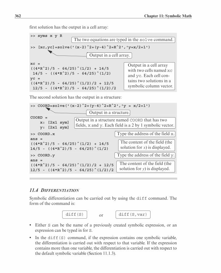
362 Chapter 11: Symbolic Math
first solution has the output in a cell array:
The second solution has the output in a structure:
11.4 DIFFERENTIATION
Symbolic differentiation can be carried out by using the diff command. Theform of the command is:
• Either S can be the name of a previously created symbolic expression, or anexpression can be typed in for S.
• In the diff(S) command, if the expression contains one symbolic variable,the differentiation is carried out with respect to that variable. If the expressioncontains more than one variable, the differentiation is carried out with respect tothe default symbolic variable (Section 11.1.3).
>> syms x y R
>> [xc,yc]=solve('(x-2)^2+(y-4)^2=R^2','y=x/2+1')
xc =((4*R^2)/5 - 64/25)^(1/2) + 14/5 14/5 - ((4*R^2)/5 - 64/25)^(1/2)yc =((4*R^2)/5 - 64/25)^(1/2)/2 + 12/5 12/5 - ((4*R^2)/5 - 64/25)^(1/2)/2
>> COORD=solve('(x-2)^2+(y-4)^2=R^2','y = x/2+1')
COORD = x: [2x1 sym] y: [2x1 sym]
>> COORD.xans =((4*R^2)/5 - 64/25)^(1/2) + 14/514/5 - ((4*R^2)/5 - 64/25)^(1/2)
>> COORD.yans =((4*R^2)/5 - 64/25)^(1/2)/2 + 12/512/5 - ((4*R^2)/5 - 64/25)^(1/2)/2
The two equations are typed in the solve command.
Output in a cell array.
Output in a cell array with two cells named xc and yc. Each cell con-tains two solutions in a symbolic column vector.
Output in a structure.
Output in a structure named COORD that has two fields, x and y. Each field is a 2 by 1 symbolic vector.
Type the address of the field x.
The content of the field (the solution for x) is displayed.
Type the address of the field y.
The content of the field (the solution for y) is displayed.
diff(S) diff(S,var)or

11.5 Integration 363
• In the diff(S,var) command (which is used for differentiation of expres-sions with several symbolic variables) the differentiation is carried out withrespect to the variable var.
• The second or higher (nth) derivative can be determined with the diff(S,n)or diff(S,var,n) command, where n is a positive number. n = 2 for the sec-ond derivative, n = 3 for the third, and so on.
Some examples are:
• It is also possible to use the diff command by typing the expression to be dif-ferentiated as a string directly in the command without having the variables inthe expression first created as symbolic objects. However, the variables in the dif-ferentiated expression do not exist as independent symbolic objects.
11.5 INTEGRATION
Symbolic integration can be carried out by using the int command. The com-mand can be used for determining indefinite integrals (antiderivatives) and defi-nite integrals. For indefinite integration the form of the command is:
>> syms x y t
>> S=exp(x^4);
>> diff(S)
ans =4*x^3*exp(x^4)
>> diff((1-4*x)^3)
ans =-12*(1-4*x)^2
>> R=5*y^2*cos(3*t);
>> diff(R)
ans =10*y*cos(3*t)
>> diff(R,t)
ans =-15*y^2*sin(3*t)
>> diff(S,2)
ans =12*x^2*exp(x^4)+16*x^6*exp(x^4)
Define x, y, and t as symbolic variables.
Assign to S the expression .ex4
Use the diff(S)command to differentiate S.
The answer is displayed.4x3ex4
Use the diff(S)command to differentiate .
The answer is displayed.
Assign to R the expression .5y2 3tcos
Use the diff(R)command to differentiate R.MATLAB differentiates R with respect to y (default symbolic variable); the answer is displayed.10y 3tcos
Use the diff(R,t)command to differentiate R w.r.t. t.
The answer is displayed.
Use diff(S,2)command to obtain the second derivative of S.
The answer is displayed.
12x2ex4 16x6ex4+
int(S) int(S,var)or

364 Chapter 11: Symbolic Math
• Either S can be the name of a previously created symbolic expression, or anexpression can be typed in for S.
• In the int(S) command, if the expression contains one symbolic variable, theintegration is carried out with respect to that variable. If the expression containsmore than one variable, the integration is carried out with respect to the defaultsymbolic variable (Section 11.1.3).
• In the int(S,var) command, which is used for integration of expressionswith several symbolic variables, the integration is carried out with respect to thevariable var.
Some examples are:
For definite integration the form of the command is:
• a and b are the limits of integration. The limits can be numbers or symbolic
variables.
For example, determination of the definite integral with
MATLAB is:
>> syms x y t
>> S=2*cos(x)-6*x;
>> int(S)
ans =2*sin(x)-3*x^2
>> int(x*sin(x))
ans =sin(x)-x*cos(x)
>>R=5*y^2*cos(4*t);
>> int(R)
ans =(5*y^3*cos(4*t))/3
>> int(R,t)
ans =(5*y^2*sin(4*t))/4
>> syms y
>> int(sin(y)-5*y^2,0,pi)
ans =2 - (5*pi^3)/3
Define x, y, and t as symbolic variables.
Assign to S the expression .Use the int(S)command to integrate S.
The answer is displayed.
Use the int(S)command to integrate .x xsin
The answer is displayed.
Assign to R the expression .5y2 4tcos
Use the int(R)command to integrate R.MATLAB integrates R with respect to y (default sym-bolic variable); the answer is displayed.
Use the int(R,t)command to integrate R w.r.t. t.
The answer is displayed.
int(S,a,b) int(S,var,a,b)or
0
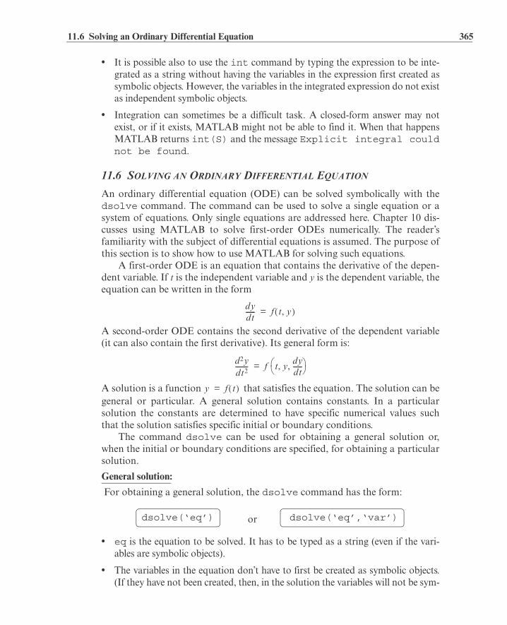
11.6 Solving an Ordinary Differential Equation 365
• It is possible also to use the int command by typing the expression to be inte-grated as a string without having the variables in the expression first created assymbolic objects. However, the variables in the integrated expression do not existas independent symbolic objects.
• Integration can sometimes be a difficult task. A closed-form answer may notexist, or if it exists, MATLAB might not be able to find it. When that happensMATLAB returns int(S) and the message Explicit integral couldnot be found.
11.6 SOLVING AN ORDINARY DIFFERENTIAL EQUATION
An ordinary differential equation (ODE) can be solved symbolically with thedsolve command. The command can be used to solve a single equation or asystem of equations. Only single equations are addressed here. Chapter 10 dis-cusses using MATLAB to solve first-order ODEs numerically. The reader’sfamiliarity with the subject of differential equations is assumed. The purpose ofthis section is to show how to use MATLAB for solving such equations.
A first-order ODE is an equation that contains the derivative of the depen-dent variable. If t is the independent variable and y is the dependent variable, theequation can be written in the form
A second-order ODE contains the second derivative of the dependent variable(it can also contain the first derivative). Its general form is:
A solution is a function that satisfies the equation. The solution can begeneral or particular. A general solution contains constants. In a particularsolution the constants are determined to have specific numerical values suchthat the solution satisfies specific initial or boundary conditions.
The command dsolve can be used for obtaining a general solution or,when the initial or boundary conditions are specified, for obtaining a particularsolution.
General solution:
For obtaining a general solution, the dsolve command has the form:
• eq is the equation to be solved. It has to be typed as a string (even if the vari-ables are symbolic objects).
• The variables in the equation don’t have to first be created as symbolic objects.(If they have not been created, then, in the solution the variables will not be sym-
dydt------ f t y,=
d2ydt2-------- f t y
dydt------, ,=
y f t=
dsolve(‘eq’) dsolve(‘eq’,‘var’)or
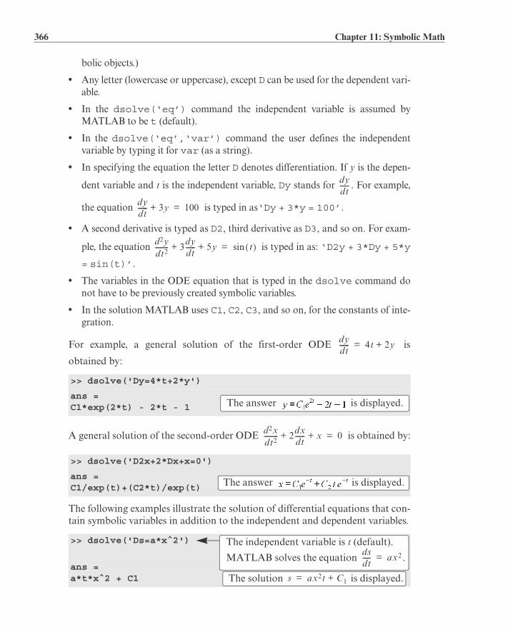
366 Chapter 11: Symbolic Math
bolic objects.)
• Any letter (lowercase or uppercase), except D can be used for the dependent vari-able.
• In the dsolve(‘eq’) command the independent variable is assumed byMATLAB to be t (default).
• In the dsolve(‘eq’,‘var’) command the user defines the independentvariable by typing it for var (as a string).
• In specifying the equation the letter D denotes differentiation. If y is the depen-
dent variable and t is the independent variable, Dy stands for . For example,
the equation is typed in as‘Dy + 3*y = 100’.
• A second derivative is typed as D2, third derivative as D3, and so on. For exam-
ple, the equation is typed in as: ‘D2y + 3*Dy + 5*y
= sin(t)’.
• The variables in the ODE equation that is typed in the dsolve command donot have to be previously created symbolic variables.
• In the solution MATLAB uses C1, C2, C3, and so on, for the constants of inte-gration.
For example, a general solution of the first-order ODE is
obtained by:
A general solution of the second-order ODE is obtained by:
The following examples illustrate the solution of differential equations that con-tain symbolic variables in addition to the independent and dependent variables.
>> dsolve('Dy=4*t+2*y')
ans =C1*exp(2*t) - 2*t - 1
>> dsolve('D2x+2*Dx+x=0')
ans =C1/exp(t)+(C2*t)/exp(t)
>> dsolve('Ds=a*x^2')
ans =a*t*x^2 + C1
dydt------
dydt------ 3y+ 100=
d2ydt2-------- 3dy
dt------ 5y+ + tsin=
dydt------ 4t 2y+=
The answer is displayed.
d2xdt2--------- 2dx
dt------ x+ + 0=
The answer is displayed.
The independent variable is t (default).
MATLAB solves the equation .dsdt----- ax2=
The solution is displayed.s ax2t C1+=

11.6 Solving an Ordinary Differential Equation 367
Particular solution:
A particular solution of an ODE can be obtained if boundary (or initial) condi-tions are specified. A first-order equation requires one condition, a second-order equation requires two conditions, and so on. For obtaining a particularsolution, the dsolve command has the form
• For solving equations of higher order, additional boundary conditions have tobe entered in the command. If the number of conditions is less than the order ofthe equation, MATLAB returns a solution that includes constants of integration(C1, C2, C3, and so on).
• The boundary conditions are typed in as strings in the following:
Math form MATLAB form‘y(a)=A’
‘Dy(a)=A’
‘D2y(a)=A’
• The argument ‘var’ is optional and is used to define the independent variablein the equation. If none is entered, the default is t.
For example, the first-order ODE , with the initial condition
is solved with MATLAB by:
>> dsolve('Ds=a*x^2','x')
ans =(a*x^3)/3 + C1
>> dsolve('Ds=a*x^2','a')
ans =(a^2*x^2)/2 + C2
>> dsolve('Dy+4*y=60','y(0)=5')
ans =15 - 10/exp(4*t)
The independent variable is defined to be x.
MATLAB solves the equation .dsdx------ ax2=
The solution is displayed.s13---ax3 C1+=
The independent variable is defined to be a.
MATLAB solves the equation .dsda------ ax2=
The solution is displayed.s12---a2x2 C1+=
dsolve(‘eq’,‘cond1’,‘var’)
dsolve(‘eq’,‘cond1’,‘cond2’,....,‘var’)
First-order ODE:
Higher-order ODE:
y a A=
y a A=
y a A=
dydt------ 4y+ 60=
y 0 5=
The answer is displayed.

368 Chapter 11: Symbolic Math
The second-order ODE , , , can be
solved with MATLAB by:
Additional examples of solving differential equations are shown in SampleProblem 11-5.
If MATLAB cannot find a solution, it returns an empty symbolic objectand the message Warning: explicit solution could not befound.
11.7 PLOTTING SYMBOLIC EXPRESSIONS
In many cases, there is a need to plot a symbolic expression. This can easily bedone with the ezplot command. For a symbolic expression S that containsone variable var, MATLAB considers the expression to be a function ,and the command creates a plot of versus var. For a symbolic expressionthat contains two symbolic variables var1 and var2, MATLAB considers theexpression to be a function in the form , and the commandcreates a plot of one variable versus the other.
To plot a symbolic expression S that contains one or two variables, theezplot command is:
• S is the symbolic expression to be plotted. It can be the name of a previously cre-ated symbolic expression, or an expression can be typed in for S.
• It is also possible to type the expression to be plotted as a string without havingthe variables in the expression first created as symbolic objects.
• If S has one symbolic variable, a plot of versus is created, with thevalues of var (the independent variable) on the abscissa (horizontal axis), and thevalues of on the ordinate (vertical axis).
>> dsolve('D2y-2*Dy+2*y=0','y(0)=1','Dy(0)=0')
ans =exp(t)*cos(t)-exp(t)*sin(t)
>> factor(ans)
ans =exp(t)*(cos(t)-sin(t))
y 0 1= dydt------
t 0=0=
The answer is displayed.
The answer can be simplified with the factor command.
The simplified answer is displayed.
S varS var
S var1 var2, 0=
ezplot(S)
ezplot(S,[min,max])
ezplot(S,[xmin,xmax,ymin,ymax])
or
or
Domain of independent variable.
Domain of dependent variable.
S var var
S var
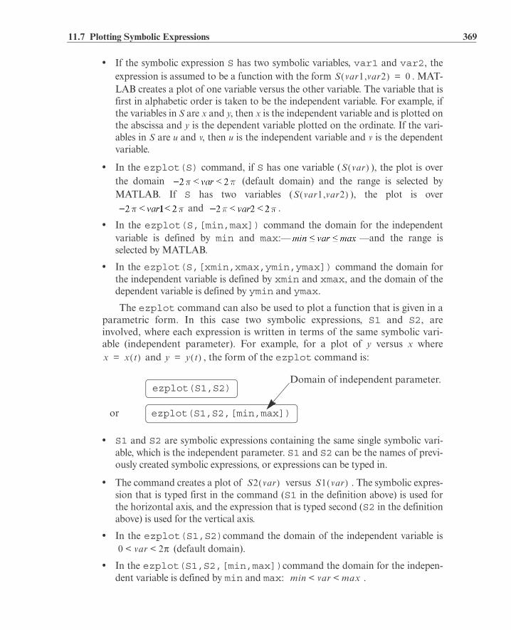
11.7 Plotting Symbolic Expressions 369
• If the symbolic expression S has two symbolic variables, var1 and var2, theexpression is assumed to be a function with the form . MAT-LAB creates a plot of one variable versus the other variable. The variable that isfirst in alphabetic order is taken to be the independent variable. For example, ifthe variables in S are x and y, then x is the independent variable and is plotted onthe abscissa and y is the dependent variable plotted on the ordinate. If the vari-ables in S are u and v, then u is the independent variable and v is the dependentvariable.
• In the ezplot(S) command, if S has one variable ( ), the plot is overthe domain (default domain) and the range is selected byMATLAB. If S has two variables ( ), the plot is over
and .
• In the ezplot(S,[min,max]) command the domain for the independentvariable is defined by min and max:— —and the range isselected by MATLAB.
• In the ezplot(S,[xmin,xmax,ymin,ymax]) command the domain forthe independent variable is defined by xmin and xmax, and the domain of thedependent variable is defined by ymin and ymax.
The ezplot command can also be used to plot a function that is given in aparametric form. In this case two symbolic expressions, S1 and S2, areinvolved, where each expression is written in terms of the same symbolic vari-able (independent parameter). For example, for a plot of y versus x where
and , the form of the ezplot command is:
• S1 and S2 are symbolic expressions containing the same single symbolic vari-able, which is the independent parameter. S1 and S2 can be the names of previ-ously created symbolic expressions, or expressions can be typed in.
• The command creates a plot of versus . The symbolic expres-sion that is typed first in the command (S1 in the definition above) is used forthe horizontal axis, and the expression that is typed second (S2 in the definitionabove) is used for the vertical axis.
• In the ezplot(S1,S2)command the domain of the independent variable is (default domain).
• In the ezplot(S1,S2,[min,max])command the domain for the indepen-dent variable is defined by min and max: .
S var1 var2, 0=
S var
S var1 var2,
x x t= y y t=
ezplot(S1,S2)
ezplot(S1,S2,[min,max])or
Domain of independent parameter.
S2 var S1 var
0 var 2< <
min var max< <
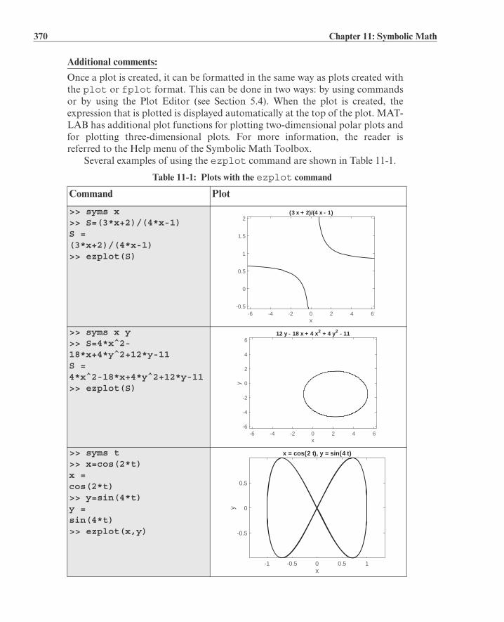
370 Chapter 11: Symbolic Math
Additional comments:
Once a plot is created, it can be formatted in the same way as plots created withthe plot or fplot format. This can be done in two ways: by using commandsor by using the Plot Editor (see Section 5.4). When the plot is created, theexpression that is plotted is displayed automatically at the top of the plot. MAT-LAB has additional plot functions for plotting two-dimensional polar plots andfor plotting three-dimensional plots. For more information, the reader isreferred to the Help menu of the Symbolic Math Toolbox.
Several examples of using the ezplot command are shown in Table 11-1.
Table 11-1: Plots with the ezplot command
Command Plot
>> syms x>> S=(3*x+2)/(4*x-1)S =(3*x+2)/(4*x-1)>> ezplot(S)
>> syms x y>> S=4*x^2-18*x+4*y^2+12*y-11S =4*x^2-18*x+4*y^2+12*y-11>> ezplot(S)
>> syms t>> x=cos(2*t)x =cos(2*t)>> y=sin(4*t)y =sin(4*t)>> ezplot(x,y)
-6 -4 -2 0 2 4 6x
-0.5
0
0.5
1
1.5
2(3 x + 2)/(4 x - 1)
12 y - 18 x + 4 x2 + 4 y2 - 11
-6 -4 -2 0 2 4 6x
-6
-4
-2
0
2
4
6
y
-1 -0.5 0 0.5 1x
-0.5
0
0.5
y
x = cos(2 t), y = sin(4 t)

11.8 Numerical Calculations with Symbolic Expressions 371
11.8 NUMERICAL CALCULATIONS WITH SYMBOLIC EXPRESSIONS
Once a symbolic expression is created by the user or by the output from any ofMATLAB’s symbolic operations, there may be a need to substitute numbers forthe symbolic variables and calculate the numerical value of the expression. Thiscan be done by using the subs command. The subs command has severalforms and can be used in different ways. The following describes several formsthat are easy to use and are suitable for most applications. In one form, the vari-able (or variables) for which a numerical value is substituted and the numericalvalue itself are typed inside the subs command. In another form, each variableis assigned a numerical value in a separate command and then the variable issubstituted in the expression.
The subs command in which the variable and its value are typed inside thecommand is shown first. Two cases are presented—one for substituting anumerical value (or values) for one symbolic variable, and the other for substi-tuting numerical values for two or more symbolic variables.
Substituting a numerical value for one symbolic variable:
A numerical value (or values) can be substituted for one symbolic variable whena symbolic expression has one or more symbolic variables. In this case the subscommand has the form:
• number can be one number (a scalar), or an array with many elements (a vectoror a matrix).
• The value of S is calculated for each value of number and the result is assignedto R, which will have the same size as number (scalar, vector, or matrix).
• If S has one variable, the output R is numerical. If S has several variables and anumerical value is substituted for only one of them, the output R is a symbolicexpression.
An example with an expression that includes one symbolic variable is:
>> syms x
>> S=0.8*x^3+4*exp(0.5*x)
S =4*exp(x/2) + (4*x^3)/5
>> SD=diff(S)
The name of thesymbolic expression.
The variable for which a numerical value is substituted.
The numerical value (or values) assigned to var.
R = subs(S,var,number)
Define x as a symbolic variable.
Assign to S the expression.0.8x3 4e 0.5x+
Use the diff(S)command to differentiate S.

372 Chapter 11: Symbolic Math
In the last example, notice that when the numerical value of the symbolicexpression is calculated, the answer is numerical (the display is indented). Anexample of substituting numerical values for one symbolic variable in an expres-sion that has several symbolic variables is:
Substituting a numerical value for two or more symbolic variables:
A numerical value (or values) can be substituted for two or more symbolic vari-ables when a symbolic expression has several symbolic variables. In this case thesubs command has the following form (it is shown for two variables, but it canbe used in the same form for more):
SD =2*exp(x/2)+(12*x^2)/5)
>> subs(SD, x, 2)
ans = 15.0366
>> SDU=subs(SD, x, [2:0.5:4])
SDU = 15.0366 21.9807 30.5634 40.9092 53.1781
>> syms a g t v
>> Y=v^2*exp(a*t)/g
Y =v^2*exp(a*t)/g
>> subs(Y,t,2)
ans =v^2*exp(2*a)/g
>> Yt=subs(Y,t,[2:4])
Yt =[ v^2*exp(2*a)/g, v^2*exp(3*a)/g, v^2*exp(4*a)/g]
The answer is assigned to SD.
Use the subs command to substitute in SD.x 2=
The value of SD is displayed.
Use the subs command to substitute x = [2, 2.5, 3, 3.5, 4] (vector) in SD.
The values of SD (assigned to SDU) for each value of x are displayed in a vector.
Define a, g, t, and v as symbolic variables.
Create the symbolic expression
and assign it to Y.
Use the subs command to substitute in SD.t 2=
The answer is displayed.Use the subs command to substitute t = [2, 3, 4] (vector) in Y.
The answer is a vector with elements of symbolic expressions for each value of t.
The name of thesymbolic expression.
The variables for which numerical val-ues are substituted.
The numerical value (or values) assigned to var1 and var2.
R = subs(S,{var1,var2},{number1,number2})

11.8 Numerical Calculations with Symbolic Expressions 373
• The variables var1 and var2 are the variables in the expression S for which thenumerical values are substituted. The variables are typed as a cell array (insidecurly braces { }). A cell array is an array of cells where each cell can be an arrayof numbers or text.
• The numbers number1,number2 substituted for the variables are also typedas a cell array (inside curly braces { }). The numbers can be scalars, vectors, ormatrices. The first cell in the numbers cell array (number1) is substituted forthe variable that is in the first cell of the variable cell array (var1), and so on.
• If all the numbers that are substituted for variables are scalars, the outcome willbe one number or one expression (if some of the variables are still symbolic).
• If, for at least one variable, the substituted numbers are an array, the mathemati-cal operations are executed element-by-element and the outcome is an array ofnumbers or expressions. It should be emphasized that the calculations are per-formed element-by-element even though the expression S is not typed in the ele-ment-by-element notation. This also means that all the arrays substituted fordifferent variables must be of the same size.
• It is possible to substitute arrays (of the same size) for some of the variables andscalars for other variables. In this case, in order to carry out element-by-elementoperations, MATLAB expands the scalars (array of 1s times the scalar) to pro-duce an array result.
The substitution of numerical values for two or more variables is demonstratedin the next examples.
>> syms a b c e x
>> S=a*x^e+b*x+c
S =a*x^e+b*x+c
>> subs(S,{a,b,c,e,x},{5,4,-20,2,3})
ans = 37
>> T=subs(S,{a,b,c},{6,5,7})
T =5*x+ 6*x^e+7
>> R=subs(S,{b,c,e},{[2 4 6],9,[1 3 5]})
R =[ 2*x+a*x+9, a*x^3+4*x+9, a*x^5+6*x+9]
>> W=subs(S,{a,b,c,e,x},{[4 2 0],[2 4 6],[2 2 2],[1 3 5],[3 2 1]})
Define a, b, c, e, and x as symbolic variables.
Create the symbolic expression and assigned it to S.axe bx c+ +
Cell array.
Substitute in S scalars forall the symbolic variables.
Cell array.
The value of S is displayed.
Substitute in S scalars for thesymbolic variables a, b, and c.
The result is an expression with the variables x and
Substitute in S a scalar for c,and vectors for b and e.
The result is a vector of symbolic expressions.
Substitute in S vectors for all the variables.

374 Chapter 11: Symbolic Math
A second method for substituting numerical values for symbolic variables ina symbolic expression is to first assign numerical values to the variables andthen use the subs command. In this method, once the symbolic expressionexists (at which point the variables in the expression are symbolic) the variablesare assigned numerical values. Then the subs command is used in the form:
Once the symbolic variables are redefined as numerical variables they can nolonger be used as symbolic. The method is demonstrated in the following exam-ples.
11.9 EXAMPLES OF MATLAB APPLICATIONS
Sample Problem 11-2: Firing angle of a projectile
A projectile is fired at a speedof 210 m/s and an angle .The projectile’s intended tar-get is 2,600 m away and 350m above the firing point.(a) Derive the equation that
has to be solved in orderto determine the angle such that the projectile will hit the target.
W = 20 26 8
>> syms A c m x y
>> S=A*cos(m*x)+c*y
S =c*y+A*cos(m*x)
>> A=10; m=0.5; c=3;
>> subs(S)
ans =3*y + 10*cos(x/2)
>> x=linspace(0,2*pi,4);
>> T = subs(S)
T =[ 3*y+10, 3*y+5, 3*y-5, 3*y-10]
The result is a vector of numerical values.
R = subs(S) The name of thesymbolic expression.
Define A, c, m, x, and y as symbolic variables.
Create the symbolic expression and assign it to S.A mxcos cy+
Assign numerical values to variables A, m, and c.
Use the subs command with the expression S.
The numerical values of variablesA, m, and c are substituted in S.
Assign numerical values (vector) to variable x.
Use the subs command with the expression S.
The numerical values of variables A,m, c, and x are substituted. The resultis a vector of symbolic expressions.

11.9 Examples of MATLAB Applications 375
(b) Use MATLAB to solve the equation derived in part (a).(c) For the angle determined in part (b), use the ezplot command to make a
plot of the projectile’s trajectory.
Solution
(a) The motion of the projectile can be analyzed by considering the horizontaland vertical components. The initial velocity can be resolved into horizontaland vertical components:
and
In the horizontal direction the velocity is constant, and the position of the pro-jectile as a function of time is given by:
Substituting m for the horizontal distance that the projectile travelsto reach the target and for , and solving for t gives:
In the vertical direction the position of the projectile is given by:
Substituting m for the vertical coordinate of the target, for, , and t gives:
or:
The solution of this equation gives the angle at which the projectile has to befired.
(b) A solution of the equation derived in part (a) obtained by using the solvecommand (in the Command Window) is:
>> syms th
Angle = solve('2600*sqrt(1 - cos(th)^2)/cos(th) - 0.5*9.81*(2600/(210*cos(th)))^2 = 350')
Angle = 1.245354497237416168313813580656 0.45925280703207121277786452037279 -0.45925280703207121277786452037279 -1.245354497237416168313813580656
v0
v0x v0 cos= v0y v0 sin=
x v0xt=
x 2600=210cos v0x
t2600
210cos--------------------------=
y 350= 210sinv0x g 9.81=
MATLAB displays four solutions. The two posi-tive ones are relevant to the problem.

376 Chapter 11: Symbolic Math
(c) The solution from part (b) shows that there are two possible angles and thustwo trajectories. In order to make a plot of a trajectory, the x and y coordinatesof the projectile are written in terms of t (parametric form):
and
The domain for t is to .
These equations can be used in the ezplot command to make the plots shownin the following program written in a script file.
>> Angle1 = Angle(1)*180/pi
Angle1 =224.16380950273491029648644451808/pi
>> Angle1=double(Angle1)
Angle1 = 71.3536
>> Angle2=Angle(2)*180/pi
Angle2 =82.665505265772818300015613667102/pi
>> Angle2=double(Angle2)
Angle2 = 26.3132
xmax=2600; v0=210; g=9.81;
theta1=1.24535; theta2=.45925;
t1=xmax/(v0*cos(theta1));
t2=xmax/(v0*cos(theta2));
syms t
X1=v0*cos(theta1)*t;
X2=v0*cos(theta2)*t;
Y1=v0*sin(theta1)*t-0.5*g*t^2;
Y2=v0*sin(theta2)*t-0.5*g*t^2;
ezplot(X1,Y1,[0,t1])
hold on
ezplot(X2,Y2,[0,t2])
hold off
Converting the solution in the first ele-ment of Angle from radians to degrees.
MATLAB displays the answer asa symbolic object in terms of .
Use the double command to obtainnumerical values for Angle1.
Converting the solution in the second ele-ment of Angle from radians to degrees.
MATLAB displays the answer asa symbolic object in terms of .
Use the double command to obtainnumerical values for Angle2.
x v0 cos t=
t 0= t2600
210cos--------------------------=
Assign the two solutions frompart (b) to theta1 and theta2.
Plot one trajectory.
Plot a second trajectory.

11.9 Examples of MATLAB Applications 377
When this program is executed, the following plot is generated in the FigureWindow:
Sample Problem 11-3: Bending resistance of a beam
The bending resistance of a rectangular beam ofwidth b and height h is proportional to the beam’s
moment of inertia I, defined by . A rect-
angular beam is cut out of a cylindrical log of radiusR. Determine b and h (as a function of R) such thatthe beam will have maximum I.
Solution
The problem is solved by following these steps:1. Write an equation that relates R, h, and b.2. Derive an expression for I in terms of h.3. Take the derivative of I with respect to h.4. Set the derivative equal to zero and solve for h.5. Determine the corresponding b.
The first step is carried out by looking at the trianglein the figure. The relationship between R, h, and b is given by the Pythagorean
theorem as . Solving this equation for b gives .
The rest of the steps are done using MATLAB:
>> syms b h R
>> b=sqrt(4*R^2-h^2);
>> I=b*h^3/12
I =(h^3*(4*R^2-h^2)^(1/2))/12
0 500 1000 1500 2000 2500x
0
200
400
600
800
1000
1200
1400
1600
1800
2000
y
x = (6623137634930013 t)/35184372088832, y = (3275240998958541 t)/35184372088832 - (981 t2)/200
I112------bh3=
b2---
2 h2---
2+ R2=
Create a symbolic expression for b.
Step 2: Create a symbolic expression for I.
MATLAB substitutes b in I.

378 Chapter 11: Symbolic Math
Sample Problem 11-4: Fuel level in a tank
The horizontal cylindrical tank shown isused to store fuel. The tank has a diameterof 6 m and is 8 m long. The amount of fuelin the tank can be estimated by looking atthe level of the fuel through a narrow verti-cal glass window at the front of the tank. Ascale that is marked next to the windowshows the levels of the fuel correspondingto 40, 60, 80, 120, and 160 thousand liters.Determine the vertical positions (measuredfrom the ground) of the lines of the scale.
Solution
The relationship between the level of the fuel and its volume can be written inthe form of a definite integral. Once the integration is carried out, an equation isobtained for the volume in terms of the fuel’s height. The height correspondingto a specific volume can then be determined from solving the equation for theheight.
>> ID=diff(I,h)
ID =(h^2*(4*R^2-h^2)^(1/2))/4-h^4/(12*(4*R^2-h^2)^(1/2))
>> hs=solve(ID,h)
hs = 0 3^(1/2)*R -3^(1/2)*R
>> bs=subs(b,hs(2))
bs =(R^2)^(1/2)
Step 3: Use the diff(R)commandto differentiate I with respect to h.
The derivative of I is displayed.
Step 4: Use the solve command to solve the equation ID = 0 for h. Assign the answer to hs.
MATLAB displays three solutions. The positive non zero solution is relevant to the problem.3R
Step 5: Use the subs command to determine b by substituting the solution for h in the expression for
The answer for b is displayed. (The answer is R,
but MATLAB displays .)

11.9 Examples of MATLAB Applications 379
The volume of the fuel V can be determinedby multiplying the area of the cross sectionof the fuel A (the shaded area) by the lengthof the tank L. The cross-sectional area canbe calculated by integration.
The width w of the top surface of the fuelcan be written as a function of y. From thetriangle in the figure on the right, the vari-ables y, w, and R are related by:
Solving this equation for w gives:
The volume of the fuel at height h can now be calculated by substituting w in theintegral in the equation for the volume and carrying out the integration. Theresult is an equation that gives the volume V as a function of h. The value of hfor a given V is obtained by solving the equation for h. In the present problemvalues of h have to be determined for volumes of 40, 60, 80, 120, and 160 thou-sand liters. The solution is given in the following MATLAB program (scriptfile):
When the script file is executed, the outcomes from commands that don’t have a
R=3; L=8;
syms w y h
w=2*sqrt(R^2-(R-y)^2)
S = L*w
V = int(S,y,0,h)
Vscale=[40:40:200]
for i=1:5
Veq=V-Vscale(i);
h_ans(i)=solve(Veq);
end
h_scale=double(h_ans)
V AL L w yd0
h
= =
Create a symbolic expression for w.
Create the expression that will be integrated.
Use the int command to integrate S from0 to h. The result gives V as a function of h.
Create a vector with the values of V in the scale.
Each pass in the loop solves h for one value of V.
Create the equation for h that has to be solved.
Use the solve command to solve for h.
h_ans is a vector (symbolic with numbers) with the values ofh that correspond to the values of V in the vector Vscale.
Use the double command to obtain numeri-cal values for the elements of vector h_ans.

380 Chapter 11: Symbolic Math
semicolon at the end are displayed. The display in the Command Window is:
Units: The unit for length in the solution is meters, which correspond to m3 forthe volume (1 m3 = 1,000 L).
Sample Problem 11-5: Amount of medication in the body
The amount M of medication present in the body depends on the rate at whichthe medication is consumed by the body and on the rate at which the medicationenters the body, where the rate at which the medication is consumed is propor-tional to the amount present in the body. A differential equation for M is
where k is the proportionality constant and p is the rate at which the medicationis injected into the body.(a) Determine k if the half-life of the medication is 3 hours.(b) A patient is admitted to a hospital and the medication is given at a rate of 50
mg per hour. (Initially there is no medication in the patient’s body.) Derivean expression for M as a function of time.
(c) Plot M as a function of time for the first 24 hours.
Solution
(a) The proportionality constant can be determined from considering the casein which the medication is consumed by the body and no new medication isgiven. In this case the differential equation is:
The equation can be solved with the initial condition at :
>> w =2*(9-(y-3)^2)^(1/2)
S =16*(9-(y-3)^2)^(1/2)
V =36*pi+72*asin(h/3-1)+8*(9-(h-3)^2)^(1/2)*(h-3)
Vscale = 40 80 120 160 200
h_scale = 1.3972 2.3042 3.1439 3.9957 4.9608
>> syms M M0 k t
The symbolic expression for w is displayed.
S is the expression that will be integrated.
The result from the integration; V as a function of h.
The values of V in the scale are displayed.
The positions of the lines in the scale are displayed.
M M0= t 0=

11.9 Examples of MATLAB Applications 381
The solution gives M as a function of time:
A half-life of 3 hours means that at hours . Substituting this
information in the solution gives , and the constant k is determined
from solving this equation:
(b) For this part the differential equation for M is:
The constant k is known from part (a), and mg/h is given. The initialcondition is that in the beginning there is no medication in the patient’s body, or
at . The solution of this equation with MATLAB is:
(c) A plot of Mtb as a function of time for can be done by using theezplot command:
In the actual display of the last expression that was generated by MATLAB(Mtt = . . .) the numbers have many more decimal digits than shown above. Thenumbers were shortened so that they will fit on the page.The plot that is generated is:
>> Mt=dsolve('DM=-k*M','M(0)=M0')
Mt =M0/exp(k*t)
ks=solve('0.5=1/exp(k*3)')
ks =.23104906018664843647241070715273
>> syms p
>> Mtb=dsolve('DM=-k*M+p','M(0)=0')
Mtb =(p-p/exp(k*t))/k)
>> pgiven=50;
>> Mtt=subs(Mtb,{p,k},{pgiven,ks})
Mtt =216.404-216.404/exp(0.231049*t)
>> ezplot(Mtt,[0,24])
Use the dsolve command
to solve .
M tM0
ekt--------=
t 3= M t12---M
0=
0.51
e3k-------=
Use the solve command
to solve .
p 50=
M 0= t 0=
Use the dsolve command
to solve .
Substitute numerical values for p and k.

382 Chapter 11: Symbolic Math
11.10 PROBLEMS
1. Define x as a symbolic variable and create the two symbolic expressions
and
Use symbolic operations to determine the simplest form of each of the fol-lowing expressions:
(a) (b) (c)
(d) Use the subs command to evaluate the numerical value of the resultfrom part (c) for .
2. Define y as a symbolic variable and create the two symbolic expressions
and Use symbolic operations to determine the simplest form of each of the fol-lowing expressions:
(a) (b) (c)
(d) Use the subs command to evaluate the numerical value of the resultfrom part (c) for .
3. Define x and y as symbolic variables and create the two symbolic expres-sions
and
Use symbolic operations to determine the simplest form of . Use thesubs command to evaluate the numerical value of the result for and
.
0 5 10 15 20t
0
50
100
150
200
216.40425613334451110398870215028 - 216.40425613334451110398870215028 exp(-0.23104906018664843647241070715273 t)
S1
S2-----
x 7=
S1
S2-----
x 6=
x 5=y 4=

11.10 Problems 383
4. Define x as a symbolic variable.(a) Derive the equation of the polynomial that has the roots , ,
, , and .(b) Determine the roots of the polynomial:
by using the factor command.
5. Use the commands from Section 11.2 to show that:
(a)
(b)
6. Use the commands from Section 11.2 to show that:
(a)
(b)
7. In rectangular coordinates the equa-tion of the hyperbola shown in the fig-ure is given by:
(a) Use MATLAB to show that inparametric form the equation ofthe hyperbola can be written as:
and
(b) Make a plot of the hyperbola forthe domain shown in the figure by using the ezplot command.
8. A water tank has the geometry shown in the figure (theupper section is a cylinder with radius r and height h, andthe lower section is a cone with radius r and a height of2r). Determine the radius r if in. and the volume is7,000 in.3. (Write an equation for the volume in terms ofthe radius and the height. Solve the equation for theradius, and use the double command to obtain a numer-ical value.)
9. The relation between the tension T and the steady shortening velocity v in amuscle is given by the Hill equation:
where a and b are positive constants and is the isometric tension, i.e., the
x2-y2-1 = 0
-3 -2 -1 0 1 2 3x
-3
-2
-1
0
1
2
3y
h
r
2r
h 20=
T a+ v b+ T0 a+ b=T0

384 Chapter 11: Symbolic Math
tension in the muscle when . The maximum shortening velocityoccurs when .(a) Using symbolic operations, create the Hill equation as a symbolic
expression. Then use subs to substitute , and finally solve for vto show that .
(b) Use from part (a) to eliminate the constant b from the Hill equa-
tion, and show that .
10. Consider the two ellipses in the x y plane given by the equations:
and
(a) Use the ezplot command to plot the two ellipses in the same figure.(b) Determine the coordinates of the points where the ellipses intersect.
11. A 120 in.-long beam AB is attached to thewall with a pin at point A and to a 66 in.-long cable CD. A load lb isattached to the beam at point B. The ten-sion in the cable T and the x and y compo-nents of the force at A ( and ) can
be calculated from the equations:
where L and are the lengths of the beam and the cable, respectively, and dis the distance from point A to point D where the cable is attached.
(a) Use MATLAB to solve the equations for the forces T, , and in
terms of d, L, , and W. Determine given by .
(b) Use the subs command to substitute lb, in., andin. into the expressions derived in part (a). This will give the
forces as a function of the distance d. (c) Use the ezplot command to plot the forces T and (both in the
same figure as functions of d, for d starting at 20 and ending at 70 in.(d) Determine the distance d where the tension in the cable is the smallest.
Determine the value of this force.
v 0=T 0=
T 0=
vmax
d
66 in.
A
W
L
B
C
D
W 200=
FAx FAy
Lc
FAx FAy
Lc FA FA FAx2 FAy
2+=
W 200= L 120=Lc 66=
FA

11.10 Problems 385
12. A box of mass m is being pulled by a ropeas shown. The force F in the rope as afunction of x can be calculated from theequations:
where N and are the normal force and friction coefficient between the boxand surface, respectively. Consider the case where kg, m,
, and m/s2. (a) Use MATLAB to derive an expression for F, in terms of x, h, m, g, and
.(b) Use the subs command to substitute kg, m, ,
and m/s2 into the expressions that were derived in part (a).This will give the force as a function of the distance x.
(c) Use the ezplot command to plot the force F as a function of x, for xstarting at 5 and ending at 30 m.
(d) Determine the distance x where the force that is required to pull the boxis the smallest, and determine the magnitude of that force.
13. The mechanical power output P in a contracting muscle is given by:
where T is the muscle tension, v is the shortening velocity (max of ), is the isometric tension (i.e., tension at zero velocity), and k is a nondimen-sional constant that ranges between 0.15 and 0.25 for most muscles. The equation can be written in nondimensional form:
where , and . Consider the case .(a) Plot p versus u for .(b) Use differentiation to find the value of u where p is maximum.(c) Find the maximum value of p.
F
m
x
h
m 18= h 10=0.55= g 9.81=
m 18= h 10= 0.55=g 9.81=
vmax T0
k 0.25=
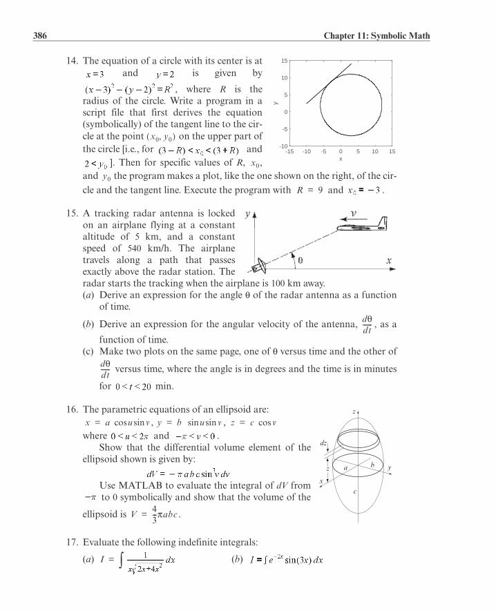
386 Chapter 11: Symbolic Math
14. The equation of a circle with its center is at and is given by
, where R is theradius of the circle. Write a program in ascript file that first derives the equation(symbolically) of the tangent line to the cir-cle at the point on the upper part ofthe circle [i.e., for and
]. Then for specific values of R, ,and the program makes a plot, like the one shown on the right, of the cir-
cle and the tangent line. Execute the program with and .
15. A tracking radar antenna is lockedon an airplane flying at a constantaltitude of 5 km, and a constantspeed of 540 km/h. The airplanetravels along a path that passesexactly above the radar station. Theradar starts the tracking when the airplane is 100 km away. (a) Derive an expression for the angle of the radar antenna as a function
of time.
(b) Derive an expression for the angular velocity of the antenna, , as a
function of time.(c) Make two plots on the same page, one of versus time and the other of
versus time, where the angle is in degrees and the time is in minutes
for min.
16. The parametric equations of an ellipsoid are:, ,
where and .Show that the differential volume element of the
ellipsoid shown is given by:
Use MATLAB to evaluate the integral of dV from to 0 symbolically and show that the volume of the
ellipsoid is .
17. Evaluate the following indefinite integrals:
(a) (b)
-15 -10 -5 0 5 10 15x
-10
-5
0
5
10
15
y
x0 y0,
x0
y0
R 9=
ddt------
ddt------
z
dz
a b
c
x
y
z
x a u vsincos= y b usin vsin= z c vcos=
V43--- abc=
I =

11.10 Problems 387
18. Define x as a symbolic variable and create the symbolic expression:
Plot S in the domain and calculate the integral .
19. The one-dimensional diffusion equation is given by:
Show that the following are solutions to the diffusion equation.
(a) , where A and B are constants.
(b) , where A, B, C, and are con-
stants.
20. A ceramic tile has the design shown in thefigure. The shaded area is painted red and therest of the tile is white. The border linebetween the red and the white areas followsthe equation:
Determine k such that the areas of the whiteand the red colors will be the same.
21. Show that the location of the centroid ofthe parabolic sector shown is given by
. The coordinate can be calculated
by:
22. Consider the parabolic sector shown in theprevious problem. Show that the moment of inertia about the x axis, , is
given by . The moment of inertia can be calculated by:
I0
=
ut
------ m2ux2
---------=
12 in.
15 in.
x
y
x
y
dy
a
h
y
x
y
a
h
yc
dAy= x2
a2hyc
yc3h5
------= yc
yc
y AdA
AdA
--------------=
Ix
Ix
Ix y2 AdA
=

388 Chapter 11: Symbolic Math
23. The rms value of an AC voltage is defined by:
where T is the period of the waveform.
(a) A voltage is given by . Show that and is
independent of . (The relationship between the period T and the radian
frequency is .)
(b) A voltage is given by V. Determine .
24. The spread of an infection from a single individual to a population of Nuninfected persons can be described by the equation:
with initial condition
where x is the number of uninfected individuals and R is a positive rate con-stant. Solve this differential equation symbolically for . Also, determinesymbolically the time t at which the infection rate dx/dt is maximum.
25. The Maxwell-Boltzmann probability density function is given by:
where m (kg) is the mass of each molecule, v (m/s) is the speed, T (K) is the
temperature, and J/K is Boltzmann’s constant. The mostprobable speed corresponds to the maximum value of and can be
determined from . Create a symbolic expression for , differ-
entiate it with respect to v, and show that . Calculate for oxy-
gen molecules ( kg) at K . Make a plot of versusv for m/s for oxygen molecules.
26. The velocity of a skydiver whose parachute isstill closed can be modeled by assuming that theair resistance is proportional to the velocity.From Newton’s second law of motion the rela-tionship between the mass m of the skydiverand his velocity v is given by (down is positive):
where c is a drag constant and g is the gravitational constant ( m/s2).
v t V tcos= vrmsV
2-------=
T2------=
v t 2.5 350t 3+cos= vrms
x 0 N=
x t
f v
vp f v
df vdv
------------- 0= f v
vp2kT
m----------= vp
T 300= f v
g 9.81=

11.10 Problems 389
(a) Solve the equation for v in terms of m, g, c, and t, assuming that the ini-tial velocity of the skydiver is zero.
(b) It is observed that 4 s after a 90-kg skydiver jumps out of an airplane, hisvelocity is 28 m/s. Determine the constant c.
(c) Make a plot of the skydiver velocity as a function of time for s.
27. A resistor R ( ) and an induc-tor L ( H) are connected asshown. Initially, the switch is connectedto point A and there is no current in thecircuit. At the switch is movedfrom A to B, so that the resistor and theinductor are connected to ( V), and current starts flowing in the circuit. The switch remainsconnected to B until the voltage on the resistor reaches 5 V. At that time( ) the switch is moved back to A.
The current i in the circuit can be calculated from solving the differen-tial equations:
during the time from and until the time when the
switch is moved back to A.
from the time when the switch is moved back to A and on.
The voltage across the resistor, , at any time is given by .
(a) Derive an expression for the current i in terms of R, L, , and t for by solving the first differential equation.
(b) Substitute the values of R, L, and in the solution for i, and determinethe time when the voltage across the resistor reaches 5 V.
(c) Derive an expression for the current i in terms of R, L, and t, for by solving the second differential equation.
(d) Make two plots (on the same page), one for versus t for and the other for versus t for .
28. Determine the general solution of the differential equation:
Show that the solution is correct. (Derive the first derivative of the solution,and then substitute back into the equation.)
29. Determine the solution of the following differential equation that satisfiesthe given initial conditions. Plot the solution for .
, ,
vS
L
RAB vR
iR 0.4=L 0.08=
t 0=
vS
vS 6=
tBA
iR Ldidt-----+ vS= t 0=
iR Ldidt-----+ 0=
vR vR iR=
vS
vS
tBA
vR
vR
dydx------ ey xcos=
y 0 2= dydx------
x 0=
3=
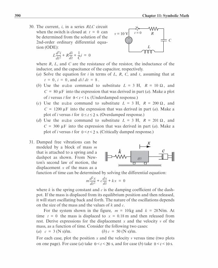
390 Chapter 11: Symbolic Math
30. The current, i, in a series RLC circuitwhen the switch is closed at canbe determined from the solution of the2nd-order ordinary differential equa-tion (ODE):
where R, L, and C are the resistance of the resistor, the inductance of theinductor, and the capacitance of the capacitor, respectively.(a) Solve the equation for i in terms of L, R, C, and t, assuming that at
, , and / .(b) Use the subs command to substitute H, , and
into the expression that was derived in part (a). Make a plotof i versus t for s. (Underdamped response.)
(c) Use the subs command to substitute H, , and into the expression that was derived in part (a). Make a
plot of i versus t for s. (Overdamped response.)(d) Use the subs command to substitute H, , and
into the expression that was derived in part (a). Make aplot of i versus t for s. (Critically damped response.)
31. Damped free vibrations can bemodeled by a block of mass mthat is attached to a spring and adashpot as shown. From New-ton’s second law of motion, thedisplacement x of the mass as afunction of time can be determined by solving the differential equation:
where k is the spring constant and c is the damping coefficient of the dash-pot. If the mass is displaced from its equilibrium position and then released,it will start oscillating back and forth. The nature of the oscillations dependson the size of the mass and the values of k and c.
For the system shown in the figure, kg and N/m. Attime the mass is displaced to m and then released fromrest. Derive expressions for the displacement x and the velocity v of themass, as a function of time. Consider the following two cases:(a) (N s)/m. (b) (N s)/m.
For each case, plot the position x and the velocity v versus time (two plotson one page). For case (a) take s, and for case (b) take s.
C
L
Rv = 10 V t = 0t 0=
Ld2idt2------- R
didt----- 1
C---- i+ + 0=
t 0= i 0= di dt 8=L 3= R 10=
C 80= F
L 3= R 200=
C 1200= F
L 3= R 201=
C 300= F
md2xdt2--------- c
dxdt------ kx+ + 0=
m 10= k 28=t 0= x 0.18=
c 3= c 50=

391
Appendix: Summary of Characters, Commands, and FunctionsThe following tables list MATLAB’s characters, commands, and functions that arecovered in the book. The items are grouped by subjects.
Characters and arithmetic operators
Character Description Page+ Addition. 11, 64– Subtraction. 11, 64* Scalar and array multiplication. 11, 65.* Element-by-element multiplication of arrays. 72/ Right division. 11, 71\ Left division. 11, 70./ Element-by-element right division. 72.\ Element-by-element left division. 72^ Exponentiation. 11.^ Element-by-element exponentiation. 72: Colon; creates vectors with equally spaced elements,
represents range of elements in arrays.37, 44
= Assignment operator. 16( ) Parentheses; sets precedence, encloses input argu-
ments in functions and subscripts of arrays.11, 42, 44, 224
[ ] Brackets; forms arrays. encloses output arguments infunctions.
37, 38, 39, 224
, Comma; separates array subscripts and functionarguments, separates commands in the same line.
9, 17, 42-45, 224
; Semicolon; suppresses display, ends row in array. 10, 39’ Single quote; matrix transpose, creates string. 41, 53-55... Ellipsis; continuation of line. 10% Percent; denotes a comment, specifies output format. 10
Relational and logical operators
Character Description Page< Less than. 176> Greater than. 176<= Less than or equal. 176

392 Summary of Characters, Commands, and Functions
>= Greater than or equal. 176== Equal. 176~= Not equal. 176& Logical AND. 179| Logical OR. 179~ Logical NOT. 179
Managing commands
Command Description Pagecd Changes current directory. 24clc Clears the Command Window. 10clear Removes all variables from the memory. 19clear x y z Removes variables x, y, and z from the memory. 19close Closes the active Figure Window. 158fclose Closes a file. 109figure Opens a Figure Window. 158fopen Opens a file. 108global Declares global variables. 227help Displays help for MATLAB functions. 226iskeyword Displays keywords. 19lookfor Search for specified word in all help entries. 226who Displays variables currently in the memory. 20, 96whos Displays information on variables in the memory. 20, 96
Predefined variables
Variable Description Pageans Value of last expression. 19eps The smallest difference between two numbers. 19i 19
inf Infinity. 19j Same as i. 19NaN Not a number. 19pi The number . 19
Display formats in the Command Window
Command Description Pageformat bank Two decimal digits. 13format compact Eliminates empty lines. 13
Relational and logical operators (Continued)
Character Description Page
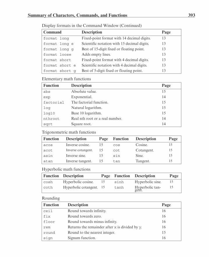
Summary of Characters, Commands, and Functions 393
format long Fixed-point format with 14 decimal digits. 13format long e Scientific notation with 15 decimal digits. 13format long g Best of 15-digit fixed or floating point. 13format loose Adds empty lines. 13format short Fixed-point format with 4 decimal digits. 13format short e Scientific notation with 4 decimal digits. 13format short g Best of 5-digit fixed or floating point. 13
Elementary math functions
Function Description Pageabs Absolute value. 15exp Exponential. 14factorial The factorial function. 15log Natural logarithm. 15log10 Base 10 logarithm. 15nthroot Real nth root or a real number. 14sqrt Square root. 14
Trigonometric math functions
Function Description Page Function Description Pageacos Inverse cosine. 15 cos Cosine. 15
acot Inverse cotangent. 15 cot Cotangent. 15
asin Inverse sine. 15 sin Sine. 15
atan Inverse tangent. 15 tan Tangent. 15
Hyperbolic math functions
Function Description Page Function Description Pagecosh Hyperbolic cosine. 15 sinh Hyperbolic sine. 15
coth Hyperbolic cotangent. 15 tanh Hyperbolic tan-gent.
15
Rounding
Function Description Pageceil Round towards infinity. 16fix Round towards zero. 16floor Round towards minus infinity. 16rem Returns the remainder after x is divided by y. 16round Round to the nearest integer. 15sign Signum function. 16
Display formats in the Command Window (Continued)
Command Description Page

394 Summary of Characters, Commands, and Functions
Creating arrays
Function Description Pagediag Creates a diagonal matrix from a vector. Creates a vec-
tor from the diagonal of a matrix.50
eye Creates a unit matrix. 40, 68linspace Creates equally spaced vector. 38ones Creates an array with ones. 40rand Creates an array with random numbers. 77, 78randi Creates an array with random integers. 78, 79randn Creates an array with normally distributed numbers. 79randperm Creates vector with permutation of integers. 78zeros Creates an array with zeros. 40
Handling arrays
Function Description Pagelength Number of elements in the vector. 49reshape Rearrange a matrix. 49size Size of an array. 49
Array functions
Function Description Pagecross Calculates cross product of two vectors. 77det Calculates determinant. 70, 77dot Calculates scalar product of two vectors. 66, 77inv Calculates the inverse of a square matrix. 69, 77max Returns maximum value. 76mean Calculates mean value. 76median Calculates median value. 76min Returns minimum value. 76sort Arranges elements in ascending order. 76std Calculates standard deviation. 77sum Calculates sum of elements. 76
Input and output
Command Description Pagedisp Displays output. 101fprintf Displays or saves output. 103-110input Prompts for user input. 99load Retrieves variables to the workspace. 112save Saves the variables in the workspace. 111uiimport Starts the Import Wizard 116

Summary of Characters, Commands, and Functions 395
xlsread Imports data from Excel 114xlswrite Exports data to Excel 115
Two-dimensional plotting
Command Description Pagebar Creates a vertical bar plot. 152barh Creates a horizontal bar plot. 152errorbar Creates a plot with error bars. 151fplot Plots a function. 140hist Creates a histogram. 153-156hold off Ends hold on. 142hold on Keeps current graph open. 142line Adds curves to existing plot. 143loglog Creates a plot with log scale on both axes. 149pie Creates a pie plot. 153plot Creates a plot. 134polar Creates a polar plot. 156semilogx Creates a plot with log scale on the x axis. 149semilogy Creates a plot with log scale on the y axis. 149stairs Creates a stairs plot. 152stem Creates a stem plot. 153
Three-dimensional plotting
Command Description Pagebar3 Creates a vertical 3-D bar plot. 331contour Creates a 2-D contour plot. 330contour3 Creates a 3-D contour plot. 330cylinder Plots a cylinder. 331mesh Creates a mesh plot. 327, 328meshc Creates a mesh and a contour plot. 329meshgrid Creates a grid for a 3-D plot. 325meshz Creates a mesh plot with a curtain. 329pie3 Creates a pie plot. 332plot3 Creates a plot. 323pol2cart Convert the polar coordinates grid to a grid in Carte-
sian coordinates.333
scatter3 Creates a scatter plot. 332sphere Plots a sphere. 331
Input and output
Command Description Page

396 Summary of Characters, Commands, and Functions
stem3 Creates a stem plot 332surf Creates a surface plot. 327, 329surfc Creates a surface and a contour plot. 329surfl Creates a surface plot with lighting. 330waterfall Creates a mesh plot with a waterfall effect. 330
Formatting plots
Command Description Pageaxis Sets limits to axes. 147colormap Sets color. 328grid Adds grid to a plot. 148, 328gtext Adds text to a plot. 145legend Adds legend to a plot. 145subplot Creates multiple plots on one page. 157text Adds text to a plot. 145title Adds title to a plot. 144view Controls the viewing direction of a 3-D plot. 333xlabel Adds label to x axis. 144ylabel Adds label to y axis. 144
Math functions (create, evaluate, solve)
Command Description Pagefeval Evaluates the value of a math function. 238fminbnd Determines the minimum of a function. 298fzero Solves an equation with one variable. 296
Numerical integration
Function Description Pagequad Integrates a function. 300quadl Integrates a function. 301trapz Integrates a function. 302
Ordinary differential equation solvers
Command Description Pageode113 Solves a first order ODE. 304ode15s Solves a first order ODE. 305ode23 Solves a first order ODE. 304ode23s Solves a first order ODE. 305
Three-dimensional plotting (Continued)
Command Description Page

Summary of Characters, Commands, and Functions 397
ode23t Solves a first order ODE. 305ode23tb Solves a first order ODE. 305ode45 Solves a first order ODE. 304
Logical Functions
Function Description Pageall Determines if all array elements are nonzero. 182and Logical AND. 181any Determines if any array elements are nonzero. 182find Finds indices of certain elements of a vector. 182not Logical NOT. 181or Logical OR. 181xor Logical exclusive OR. 182
Flow control commands
Command Description Pagebreak Terminates execution of a loop. 202case Conditionally execute commands. 189continue Terminates a pass in a loop. 202else Conditionally execute commands. 186elseif Conditionally execute commands. 187end Terminates conditional statements and loops. 184, 189,
193, 197for Repeats execution of a group of commands. 193if Conditionally execute commands. 184otherwise Conditionally execute commands. 189switch Switches among several cases based on expression. 189while Repeats execution of a group of commands. 197
Polynomial functions
Function Description Pageconv Multiplies polynomials. 265deconv Divides polynomials. 265poly Determines coefficients of a polynomial. 264polyder Determines the derivative of a polynomial. 266polyval Calculates the value of a polynomial. 262roots Determines the roots of a polynomial. 263
Ordinary differential equation solvers (Continued)
Command Description Page
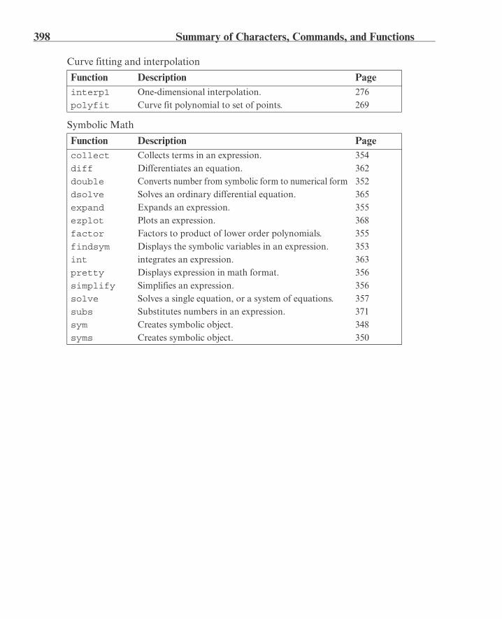
398 Summary of Characters, Commands, and Functions
Curve fitting and interpolation
Function Description Pageinterp1 One-dimensional interpolation. 276polyfit Curve fit polynomial to set of points. 269
Symbolic Math
Function Description Pagecollect Collects terms in an expression. 354diff Differentiates an equation. 362double Converts number from symbolic form to numerical form 352dsolve Solves an ordinary differential equation. 365expand Expands an expression. 355ezplot Plots an expression. 368factor Factors to product of lower order polynomials. 355findsym Displays the symbolic variables in an expression. 353int integrates an expression. 363pretty Displays expression in math format. 356simplify Simplifies an expression. 356solve Solves a single equation, or a system of equations. 357subs Substitutes numbers in an expression. 371sym Creates symbolic object. 348syms Creates symbolic object. 350
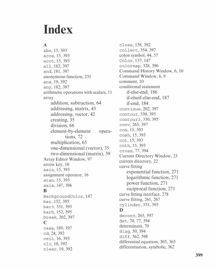
399
IndexAabs, 15, 393acos, 15, 393acot, 15, 393all, 182, 397and, 181, 397anonymous function, 231ans, 19, 392any, 182, 397arithmetic operations with scalars, 11array
addition, subtraction, 64addressing, matrix, 43addressing, vector, 42creating, 35division, 68element-by-element opera-
tions, 72multiplication, 65one-dimensional (vector), 35two-dimensional (matrix), 39
Array Editor Window, 97arrow key, 10asin, 15, 393assignment operator, 16atan, 15, 393axis, 147, 396BBackgroundColor, 147bar, 152, 395bar3, 331, 395barh, 152, 395break, 202, 397Ccase, 189, 397cd, 24, 392ceil, 16, 393clc, 10, 392clear, 19, 392
close, 158, 392collect, 354, 397colon symbol, 44, 57Color, 137, 147colormap, 328, 396Command History Window, 6, 10Command Window, 6, 9comment, 10conditional statement
if-else-end, 186if-elseif-else-end, 187if-end, 184
continue, 202, 397contour, 330, 395contour3, 330, 395conv, 265, 397cos, 15, 393cosh, 15, 393cot, 15, 393coth, 15, 393cross, 77, 394Current Directory Window, 23current directory, 22curve fitting
exponential function, 271logarithmic function, 271power function, 271reciprocal function, 271
curve fitting interface, 278curve fitting, 261, 267cylinder, 331, 395Ddeconv, 265, 397det, 70, 77, 394determinant, 70diag, 50, 394diff, 362, 398differential equation, 303, 365differentiation, symbolic, 362
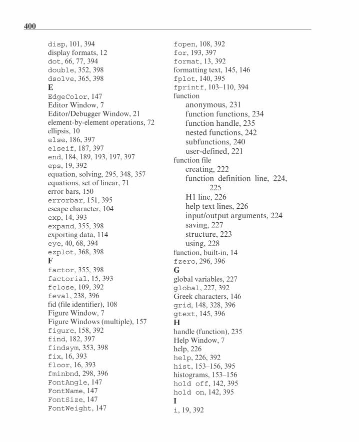
400
disp, 101, 394display formats, 12dot, 66, 77, 394double, 352, 398dsolve, 365, 398EEdgeColor, 147Editor Window, 7Editor/Debugger Window, 21element-by-element operations, 72ellipsis, 10else, 186, 397elseif, 187, 397end, 184, 189, 193, 197, 397eps, 19, 392equation, solving, 295, 348, 357equations, set of linear, 71error bars, 150errorbar, 151, 395escape character, 104exp, 14, 393expand, 355, 398exporting data, 114eye, 40, 68, 394ezplot, 368, 398Ffactor, 355, 398factorial, 15, 393fclose, 109, 392feval, 238, 396fid (file identifier), 108Figure Window, 7Figure Windows (multiple), 157figure, 158, 392find, 182, 397findsym, 353, 398fix, 16, 393floor, 16, 393fminbnd, 298, 396FontAngle, 147FontName, 147FontSize, 147FontWeight, 147
fopen, 108, 392for, 193, 397format, 13, 392formatting text, 145, 146fplot, 140, 395fprintf, 103–110, 394function
anonymous, 231function functions, 234function handle, 235nested functions, 242subfunctions, 240user-defined, 221
function filecreating, 222function definition line, 224,
225H1 line, 226help text lines, 226input/output arguments, 224saving, 227structure, 223using, 228
function, built-in, 14fzero, 296, 396Gglobal variables, 227global, 227, 392Greek characters, 146grid, 148, 328, 396gtext, 145, 396Hhandle (function), 235Help Window, 7help, 226help, 226, 392hist, 153–156, 395histograms, 153–156hold off, 142, 395hold on, 142, 395Ii, 19, 392

401
identity matrix, 68if, 184, 397Import Wizard, 116importing a function, 237importing data, 114indefinite loop, 198inf, 19, 392input a string, 100input, 99, 394int, 363, 398integration, numerical, 300integration, symbolic, 363interp1, 276, 397interpolation
cubic spline, 276linear, 276nearest, 276
interpolation, 274inv, 69, 77, 394inverse, matrix, 69iskeyword, 19, 392Jj, 19, 392Lleast squares, 268left division, 70legend, 145, 396length, 49, 394line, 143, 395linestyle, 137LineWidth, 147linewidth, 137linspace, 38, 394load, 112, 394log, 15, 393log10, 15, 393logical array, 176logical operator, 179logical vectors, 178loglog, 149, 395lookfor, 226, 392loop
for-end, 192
nested, 200while, 197
Mmarker, 137markeredgecolor, 137markerfacecolor, 137markersize, 137matrix
adding elements, 47deleting elements, 48determinant, 70identity, 68inverse, 69size of, 39
max, 76, 394mean, 76, 394median, 76, 394mesh, 327, 328, 395meshc, 329, 395meshgrid, 325, 395meshz, 329, 395M-file, 21, 231min, 76, 394modifiers, text, 146multiple Figure Windows, 157NNaN, 19, 392nested functions, 242nested loops, 200not, 181, 397nthroot, 14, 393number format, 105Oode113, 304, 396ode15s, 305, 396ode23, 304, 396ode23s, 305, 396ode23t, 305, 396ode23tb, 305, 396ode45, 304, 396ones, 40, 394or, 181, 397

402
order of precedence, 11, 178, 180otherwise, 189, 397output commands, 100output to a file, 108Ppassing a function, 237percent symbol, 10pi, 19, 392pie, 153, 395pie3, 332, 395plot
axis label, 144axis range, 147bar plot (3-D), 331bar plot, 152color specifiers, 136contour plot (2-D), 330contour plot (3-D), 330cylinder, 331error bars, 150formatting, 144–148grid for 3-D plot, 325grid, 148histograms, 153–156legend, 145line (3-D), 323line specifiers, 135, 137logarithmic axes, 149marker specifiers, 136mesh (3-D), 327mesh and contour plot (3-D),
329mesh curtain plot (3-D), 329mesh plot (3-D), 328multiple graphs in a plot, 141–
144multiple plots on a page, 157,
159pie charts, 153pie plot (3-D), 332Plot Editor, 148
plot viewing direction (3-D),333
polar plot, 156properties, 136scatter plot (3-D), 332special graphics, 152specifiers, 136stair plot, 152stem plot (3-D), 332stem plot, 152surface plot (3-D), 327, 329surface with lighting plot (3-
D), 330symbolic expression, 368text, 145three-dimensional, 323title, 144waterfall plot (3-D), 330
plot, 134, 395plot3, 323, 395Plots Toolstrip, 159plotting a function, 139–141pol2cart, 333, 395polar plot, 156polar, 156, 395poly, 264, 397polyder, 266, 397polyfit, 269, 397polynomial
addition, 264derivative, 266division, 265MATLAB representation,
261multiplication, 265roots, 263value of, 262
polyval, 262, 397pretty, 356, 398property name, 137, 146property value, 137, 146

403
Qquad, 300, 396quadl, 301, 396Rrand, 77, 78, 394randi, 78, 79, 394randn, 79, 394random numbers, 77randperm, 78, 394relational operator, 176rem, 16, 393reshape, 49, 394right division, 71roots, 263, 397Rotation, 147round, 15, 393Ssave, 111, 394saving the workspace, 111scatter3, 332, 395script file
creating, 21, 222input to, 97–100output from, 100–110running, 22saving, 22
script file, 20semicolon, 10, 17semilogx, 149, 395semilogy, 149, 395sign, 16, 393simplify, 356, 398sin, 15, 393sinh, 15, 393size, 49, 394solve, 357, 398sort, 76, 394sphere, 331, 395sqrt, 14, 393stairs, 152, 395std, 77, 394stem, 153, 395stem3, 332, 395
stopping indefinite loop, 198string, input, 100strings, 53–55subfunctions, 240subplot, 157, 396subs, 371, 398subscript, 146sum, 76, 394superscript, 146surf, 327, 329, 395surfc, 329, 395surfl, 330, 396switch, 189, 397switch-case statement, 189sym, 348, 398symbolic math
default variable, 353differential equation solution,
365differentiation, 362equation solving, 357expression, 350integration, 363numerical calculations with,
371object, 348plotting expression, 368variable, 349, 350
syms, 350, 398Ttable, display, 86, 102tan, 15, 393tanh, 15, 393text modifiers, 146text, 145, 396title, 144, 396Toolstrip, 5, 159transpose operator, 41trapz, 302, 396truth table, 183Uuiimport, 116, 394
404
Vvariable
defining, matrix, 39–41defining, scalar, 16defining, vector, 36–38global, 227local, 226name, 18predefined, 19
vectoradding elements, 46constant spacing, 37, 38creating, 36deleting elements, 48
vectorization, 75view, 333, 396Wwaterfall, 330, 396while, 197, 397who, 20, 96, 392whos, 20, 96, 392Workspace Window, 97workspace, 96Xxlabel, 144, 396xlsread, 114, 394xlswrite, 115, 395xor, 182, 397Yylabel, 144, 396Zzeros, 40, 394

WILEY END USER LICENSE AGREEMENTGo to www.wiley.com/go/eula to access Wiley’s ebook EULA.
Related Documents


