matlab

INTRODUCTION TO MATLAB

MATLAB

MATLAB is the high-level language and interactive environment developed by

MATHWORKS. It is exclusively used by engineers to explore and visualize ideas and

collaborate across disciplines including signal and image processing, communications,

control systems, and computational finance MATLAB allows matrix manipulations,

plotting of functions and data, implementation of algorithms, creation of user

interfaces, and interfacing with programs written in other languages like C++ ,

FORTRAN etc

SYNTAX

The MATLAB application is built around the MATLAB scripting language. Common

usage of the MATLAB application involves using the Command Window as an

interactive mathematical shell or executing text files containing MATLAB code.

VARIABLES

Variables are defined using the assignment operator, = . MATLAB is a weakly

typed programming language because types are implicitly converted. It is an inferred

typed language because variables can be assigned without declaring their type, except

if they are to be treated as symbolic objects, and that their type can change. Values

can come from constants, from computation involving values of other variables, or

from the output of a function.

For example:

>> x = 17

x =

17

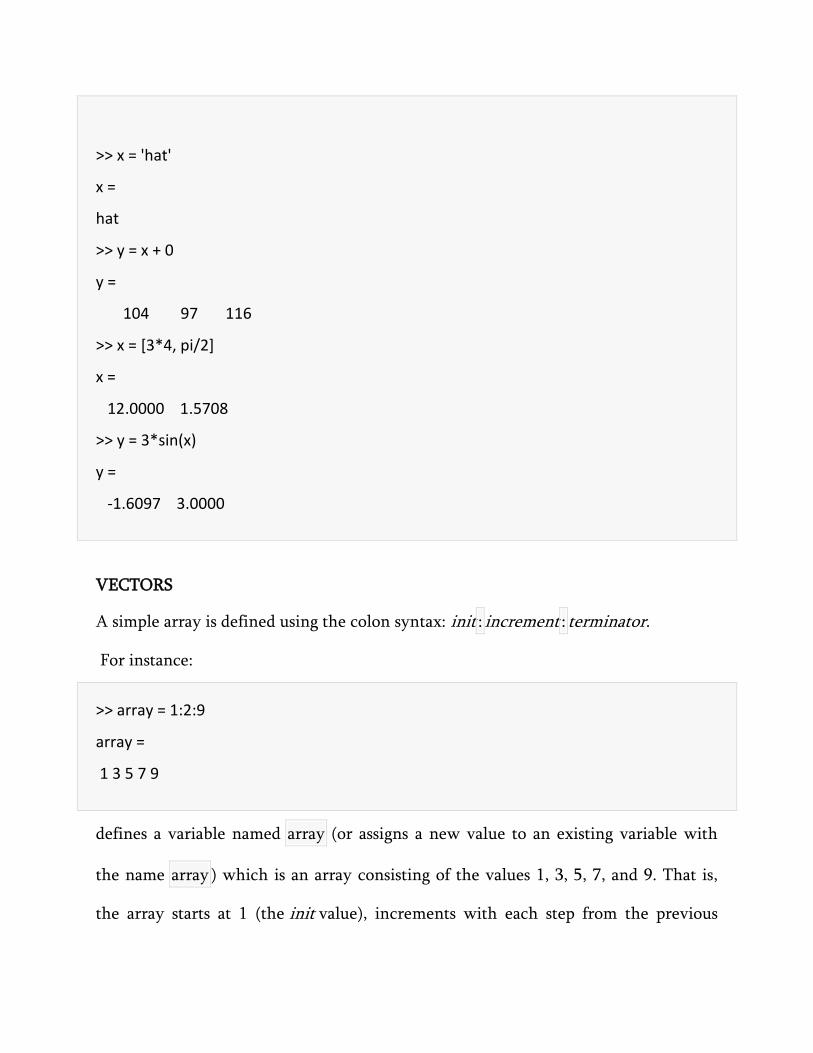
>> x = 'hat'

x =

hat

>> y = x + 0

y =

104 97 116

>> x = [3*4, pi/2]

x =

12.0000 1.5708

>> y = 3*sin(x)

y =

-1.6097 3.0000

VECTORS

A simple array is defined using the colon syntax: init : increment : terminator.

For instance:

>> array = 1:2:9

array =

1 3 5 7 9

defines a variable named array (or assigns a new value to an existing variable with

the name array ) which is an array consisting of the values 1, 3, 5, 7, and 9. That is,

the array starts at 1 (the init value), increments with each step from the previous

value by 2 (the increment value), and stops once it reaches (or to avoid exceeding) 9

(the terminator value).

>> array = 1:3:9

array =

1 4 7

the increment value can actually be left out of this syntax (along with one of the

colons), to use a default value of 1.

>> ari = 1:5

ari =

1 2 3 4 5

assigns to the variable named ari an array with the values 1, 2, 3, 4, and 5, since the

default value of 1 is used as the increment value.

Matrices can be defined by separating the elements of a row with blank space or

comma and using a semicolon to terminate each row. The list of elements should be

surrounded by square brackets: [ ]. Parentheses: ( ) are used to access elements and

subarrays (they are also used to denote a function argument list).

>> A = [16 3 2 13; 5 10 11 8; 9 6 7 12; 4 15 14 1]

A =

16 3 2 13

5 10 11 8

9 6 7 12

4 15 14 1

>> A(2,3)

ans =

11

A square identity matrix of size n can be generated using the function eye, and

matrices of any size with zeros or ones can be generated with the

functions zeros and ones, respectively.

>> eye(3,3)

ans =

1 0 0

0 1 0

0 0 1

>> zeros(2,3)

ans =

0 0 0

0 0 0

>> ones(2,3)

ans =

1 1 1

1 1 1

Exercise No 4 10/9/2015

EXERCISE ON MATLAB

1) Find the transpose, determinant, inverse, rank and Eigenvalues of the matrix.

A = 𝟐 𝟑 𝟒𝟓 𝟑 𝟐𝟐 𝟔 𝟗

Solution:

>> a = [ 2 3 4 ; 5 3 2 ; 2 6 9 ] a = 2 3 4 5 3 2 2 6 9 >> b = [a'] b = 2 5 2 3 3 6 4 2 9 >> c= det(a) c = 3 >> d = inv(a) d = 5.0000 -1.0000 -2.0000 -13.6667 3.3333 5.3333 8.0000 -2.0000 -3.0000 >> e = rank(a) e = 3 >> f = eig(a) f = 12.7650 0.2350 1.0000

2) Add the given matrices (use if and for loop statements)

A = 𝟐 𝟑 𝟒𝟓 𝟔 𝟕

and B = 𝟏 𝟐 𝟑𝟒 𝟓 𝟔

Solution:

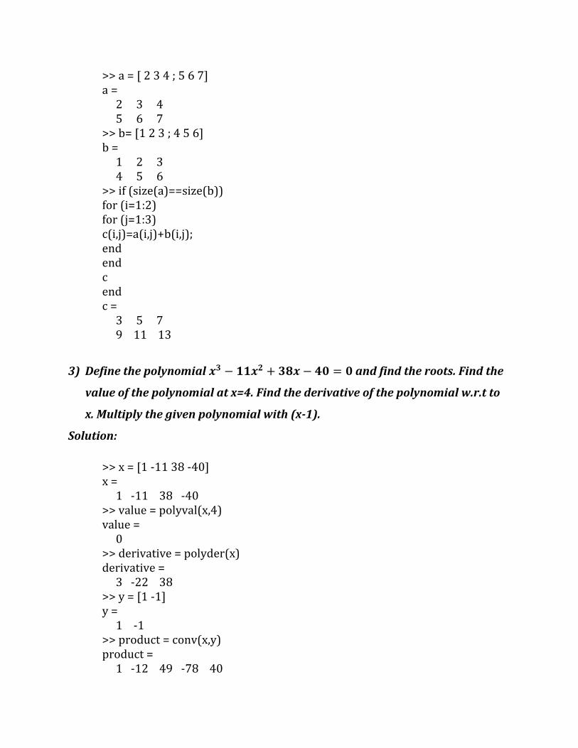
>> a = [ 2 3 4 ; 5 6 7] a = 2 3 4 5 6 7 >> b= [1 2 3 ; 4 5 6] b = 1 2 3 4 5 6 >> if (size(a)==size(b)) for (i=1:2) for (j=1:3) c(i,j)=a(i,j)+b(i,j); end end c end c = 3 5 7 9 11 13

3) Define the polynomial 𝒙𝟑 − 𝟏𝟏𝒙𝟐 + 𝟑𝟖𝒙 − 𝟒𝟎 = 𝟎 and find the roots. Find the

value of the polynomial at x=4. Find the derivative of the polynomial w.r.t to

x. Multiply the given polynomial with (x-1).

Solution:

>> x = [1 -11 38 -40] x = 1 -11 38 -40 >> value = polyval(x,4) value = 0 >> derivative = polyder(x) derivative = 3 -22 38 >> y = [1 -1] y = 1 -1 >> product = conv(x,y) product = 1 -12 49 -78 40

4) Find the polynomial whose roots are 1, 3+5i, 3-5i.

Solution:

>> x = [1 3+5i 3-5i] x = 1.0000 3.0000 + 5.0000i 3.0000 - 5.0000i >> polynomial = poly(x) polynomial = 1 -7 40 -34

5) Find the polynomial 𝟑𝒙𝟓 + 𝟐𝒙𝟒 − 𝟏𝟎𝟎𝒙𝟑 + 𝟐𝒙𝟐 − 𝟕𝒙 + 𝟗𝟎 over the range -6 ≤

𝒙 ≤ 𝟔 at a spacing of 0.01

Solution:

>> A = [3 2 -100 2 -7 90]; >> x= -6:0.01:6; >> y= polyval(A,x); >> plot(x,y); >> xlabel('x axis'); >> ylabel('y axis')

6) Plot the following functions using the subplot command.

Y = 𝒆−𝟏.𝟐𝒙 ∗ 𝒔𝒊𝒏(𝟏𝟎𝒙 + 𝟓) for 0 < 𝑥 < 5 and y = abs(𝒙𝟑 − 𝟏𝟎𝟎) for -6 <x < 6.

Solution:

>> subplot(2,1,1) >> subplot(2,1,1); >> fplot('exp(-1.2*x)*sin(10*x + 5)',[0,5]); >> xlabel('x axis 1'); >> ylabel('y axis 1'); >> subplot(2,1,2); >> fplot('abs(x^3-100)', [-6,6]); >> xlabel('x axis 2'); >> ylabel('y axis 2')

7) Evaluate ∫ 𝒔𝒊𝒏𝒙𝒅𝒙𝝅

𝟎 by the Trapezoidal and Simpson’s rules.

Solution:

>> x= 0:0.01:pi; >> y= sin(x); >> value = trapz(x,y) value = 2.0000 >> value = quad('sin(x)',0,pi) value =

2.0000

8) Solve the differential equation 𝒅𝒚

𝒅𝒙 = x+t , x0 = 0.

Solution:

>> dsolve('Dy=y+t', 'y(0)=0') ans = -t-1+exp(t)

9) Solve the system of linear equations

5x = 3y - 2z + 10

8y + 4z = 3z + 20

2x + 4y -9z = 9

Solution:

>> A=[5 -3 2; -3 8 4; 2 4 -9]

A =

5 -3 2

-3 8 4

2 4 -9

B=[10;20;9]

B =

10

20

9

>> X=inv(A)*B

X =

3.4442

3.1982

1.1868

10) Plot the following data .Then obtain the best linear fit.

x 5 10 20 50 100 y 15 33 53 140 301

Solution:

>> x= [5 10 20 50 100] x = 5 10 20 50 100 >> y=[15 33 53 140 301] y = 15 33 53 140 301 >> z=polyfit(x,y,1) z = 2.9953 -2.4264 >> b=polyval(z,x) b = 12.5502 27.5267 57.4798 147.3390 297.1044 >> plot(b,x) >> xlabel('x') >> ylabel('y')

11) Solve 𝒔𝒊𝒏𝒙 = 𝒆𝒙 − 𝟓

Solution:

>> solve('sin(x)=exp(x)-5') ans = 1.7878414746209143250134641264441

12) Perform LU decomposition of the matrix A= 𝟐 𝟑 𝟒𝟓 𝟑 𝟐𝟐 𝟔 𝟗

Solution:

>> A=[2 3 4; 5 3 2; 2 6 9] A = 2 3 4 5 3 2 2 6 9 >> [L,U,P]=lu(A) L = 1.0000 0.0000 0.0000 0.4000 1.0000 0.0000 0.4000 0.3750 1.0000 U = 5.0000 3.0000 2.0000 0.0000 4.8000 8.2000 0.0000 0.0000 0.1250 P = 0 1 0 0 0 1 1 0 0

13) Viscosity of water at different temperatures upto the normal boiling point is

listed below. Viscosity (Pa.s) = A X 10B(T-C),where T is the temperature in degree

Kelvin .

T(in Kelvin) = T (C)+273.15, C = 140 K, Find A and B.

Solution:

>> % Input the table

TempC = 10:10:100;

Viscosity = [1.31e-3, 1e-3, 7.98e-4, 6.53e-4, 5.47e-4, 4.67e-4, 4.04e-4, 3.55e-4,

3.15e-4, 2.82e-4];

figure(1)

plot(TempC,Viscosity,'r-')

xlabel('Temp (deg C)')

Temperature ( C)

10 20 30 40 50 60 70 80 90 100

Viscosity (Pa.s)

1.31 E.03

1.00 E.03

7.98 E.04

6.53 E.04

5.47 E.04

4.67 E.04

4.04 E.04

3.55 E.04

3.15 E.04

2.81 E.04

ylabel('Viscosity (Pas)')

TempK= TempC + 273.15;

figure(2)

plot(TempK, Viscosity,'r-')

% given Viscosity = A * 10^[B/(T-C)]where A and B are constants and C = 140

deg K

% take log10 on both sides. Let log10(Viscosity) = log10V

% log10V = log10(A) + B/(T-C) = a + B/(T-C)

% y = a + Bx where x = 1/(T-C)

TmC = TempK - 140;

invTmC = 1./TmC;

figure(3)

plot(TmC, Viscosity,'r-')

hold on

figure(4)

plot(invTmC, log10(Viscosity),'r-')

hold on

P = polyfit(invTmC, log10(Viscosity), 1);

Check = P(1)*invTmC + P(2);

plot(invTmC, Check,'bo')

a = P(2);

A = 10^a;

B = P(1);

CheckVis = A* 10.^(B./TmC);

figure(3)

plot(TmC,CheckVis,'bo')

xlabel('Temp - 140 (K)')

ylabel('Viscosity (Pa s)')

A

B

disp('The value of A is')

disp(A)

disp('The value of B is')

disp(B)

A =

2.4797e-05

B =

246.1846

The value of A is

2.4797e-05

The value of B is

246.1846

14) Find the viscosity of water at 25 C and 35 C using the data in the table

above using interpolation in MATLAB and validate the function obtained in the

question above.

Solution:

TempNewC = [25 35];

TempNewK = TempNewC + 273.15;

NewTmC = TempNewK - 140;

NewViscos = A* 10.^(B./NewTmC);

plot(NewTmC, NewViscos, 'g*')

disp('The viscosity at 25 and 35 deg C ')

disp(NewViscos)

The viscosity at 25 and 35 deg C

1.0e-03 *

0.8934 0.7219

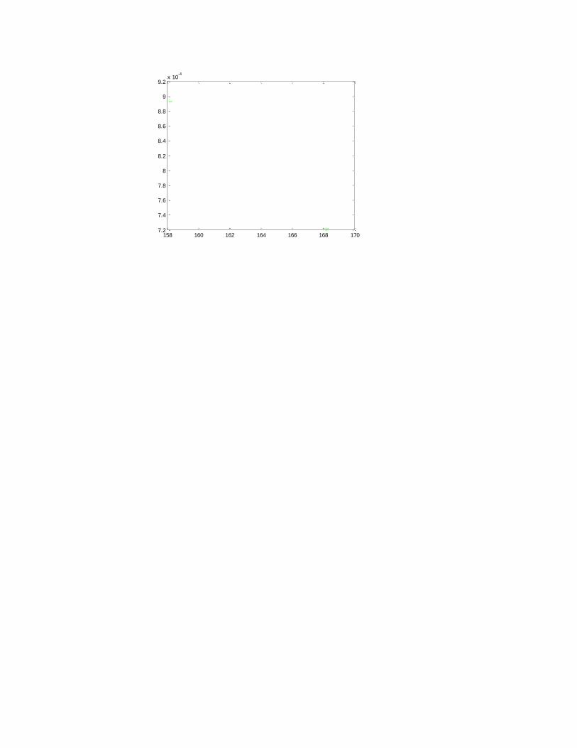
158 160 162 164 166 168 1707.2

7.4

7.6

7.8

8

8.2

8.4

8.6

8.8

9

9.2x 10

-4