MATLAB: 3-D Graphics Last revised : March, 2003MATLAB: 3-D Graphics Last revised : March, 2003 Overview To get an overview of available graphics functions in MATLAB, look at the help

M ATLAB : 3-D Graphics Last revised : March, 2003

Overview

To get an overview of available graphics functions in MATLAB , look at the help pages for the followingtopics:

graph2d Two-dimensional graphs.graph3d Three-dimensional graphs.specgraph Specialized graphs.graphics Handle graphics.

This article illustrates the use of theeasy to usegraphics commands listed under the topicspecgraph . Atthe end of the writeup two examples are given showing how one can set up the necessary data arrays to usethe more primitive commandscontour , mesh, andsurf .

ezplot Easy to use function plotter.ezplot3 Easy to use 3-D parametric curve plotter.ezcontour Easy to use contour plotter.ezcontourf Easy to use filled contour plotter.ezmesh Easy to use 3-D mesh plotter.ezmeshc Easy to use combination mesh/contour plotter.ezsurf Easy to use 3-D colored surface plotter.ezsurfc Easy to use combination surf/contour plotter.

This brief document mainly consists of examples of MATLAB code. It is suggested that you have MATLAB

running while reading so that you can verify the examples. Each of the examples includes an image of theexpected result. Just click on theView Result tag to the right of the MATLAB code.

Plotting curves: ezplot , ezplot3

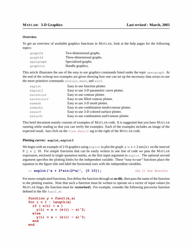
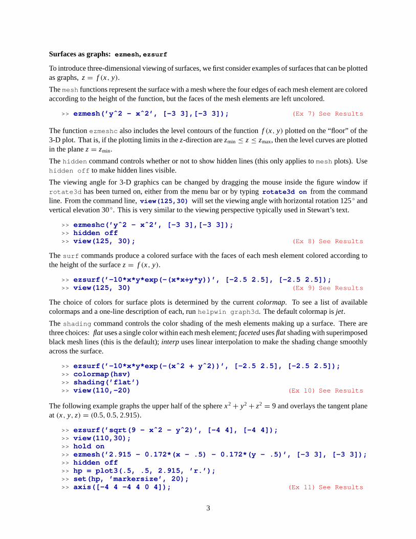
We begin with an example of 2-D graphics usingezplot to plot the graphy = x+2 sin(2x) on the interval0 ≤ x ≤ 10. For simple functions that can be easily written in one line of code we pass the MATLAB

expression, enclosed in single quotation marks, as the first input argument toezplot . The optional secondargument specifies the plotting limits for the independent variable. These “easy-to-use” functions place theequation in the figure title and label the horizontal axes with the independent variables.

>> ezplot(’x + 2*sin(2*x)’, [0 10]); (Ex 1) See Results

For more complicated functions, first define the function through anm-file, then pass the name of the functionto the plotting routine. Note that such a function must be written to operate on a vector of input values (inMATLAB lingo, the function must bevectorized). For example, consider the following piecewise functiondefined in the filefunc1.m :

function y = func1(x,a)for i = 1 : length(x)

if ( x(i) < a )y(i) = a + (x(i) - a)ˆ2;

elsey(i) = a - (x(i) - a)ˆ2;

endend

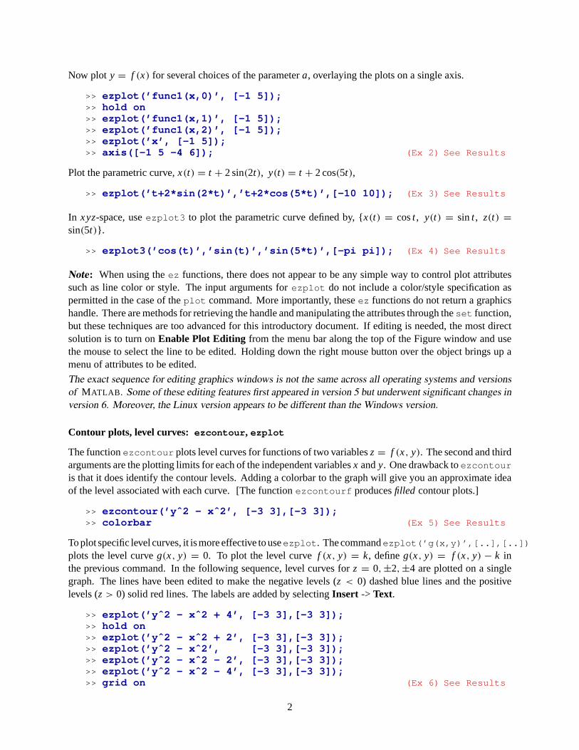
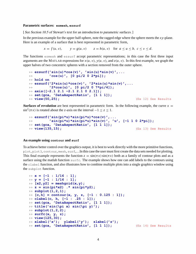
Now plot y = f (x) for several choices of the parametera, overlaying the plots on a single axis.

>> ezplot(’func1(x,0)’, [-1 5]);>> hold on>> ezplot(’func1(x,1)’, [-1 5]);>> ezplot(’func1(x,2)’, [-1 5]);>> ezplot(’x’, [-1 5]);>> axis([-1 5 -4 6]); (Ex 2) See Results

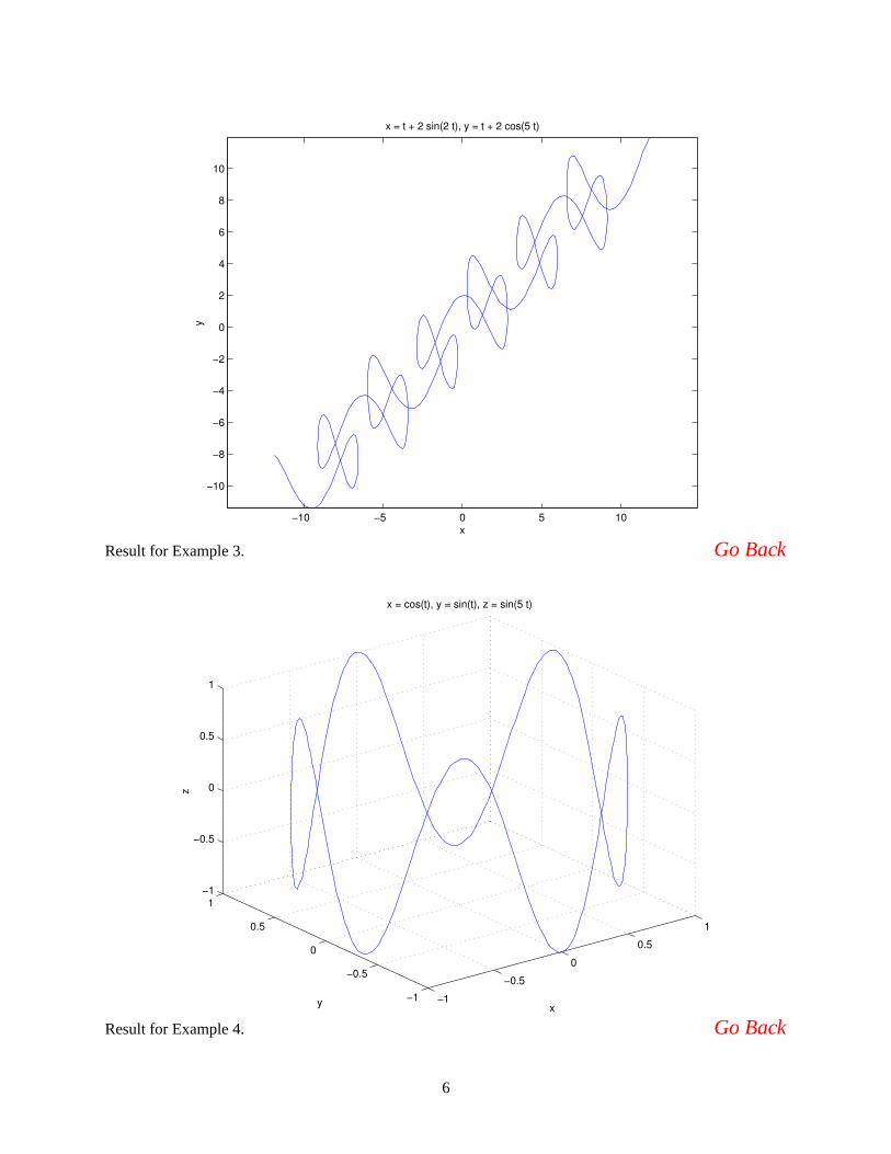
Plot the parametric curve,x(t) = t + 2 sin(2t), y(t) = t + 2 cos(5t),

>> ezplot(’t+2*sin(2*t)’,’t+2*cos(5*t)’,[-10 10]); (Ex 3) See Results

In xyz-space, useezplot3 to plot the parametric curve defined by, {x(t) = cost , y(t) = sint , z(t) =sin(5t)}.

>> ezplot3(’cos(t)’,’sin(t)’,’sin(5*t)’,[-pi pi]); (Ex 4) See Results

Note: When using theez functions, there does not appear to be any simple way to control plot attributessuch as line color or style. The input arguments forezplot do not include a color/style specification aspermitted in the case of theplot command. More importantly, theseez functions do not return a graphicshandle. There are methods for retrieving the handle and manipulating the attributes through theset function,but these techniques are too advanced for this introductory document. If editing is needed, the most directsolution is to turn onEnable Plot Editing from the menu bar along the top of the Figure window and usethe mouse to select the line to be edited. Holding down the right mouse button over the object brings up amenu of attributes to be edited.

The exact sequence for editing graphics windows is not the same across all operating systems and versionsof MATLAB . Some of these editing features first appeared in version 5 but underwent significant changes inversion 6. Moreover, the Linux version appears to be different than the Windows version.

Contour plots, level curves: ezcontour , ezplot

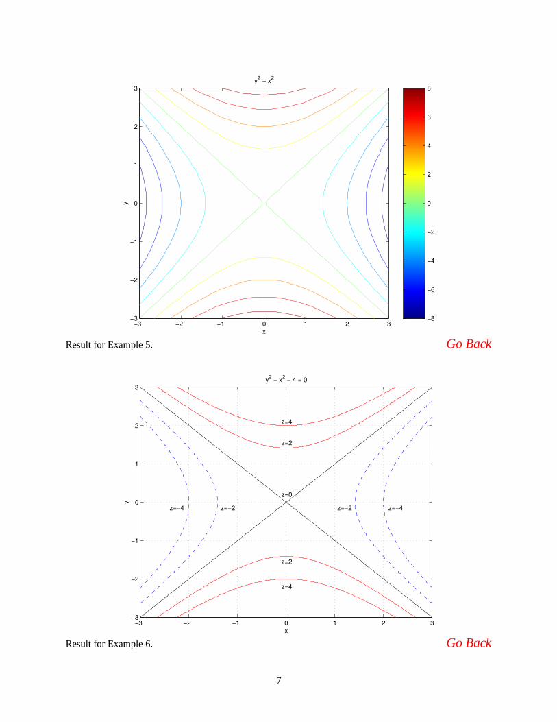
The functionezcontour plots level curves for functions of two variablesz= f (x, y). The second and thirdarguments are the plotting limits for each of the independent variablesx andy. One drawback toezcontour

is that it does identify the contour levels. Adding a colorbar to the graph will give you an approximate ideaof the level associated with each curve. [The functionezcontourf producesfilled contour plots.]

>> ezcontour(’yˆ2 - xˆ2’, [-3 3],[-3 3]);>> colorbar (Ex 5) See Results

To plot specific level curves, it is more effective to useezplot . The commandezplot(’g(x,y)’,[..],[..])

plots the level curveg(x, y) = 0. To plot the level curvef (x, y) = k, defineg(x, y) = f (x, y) − k inthe previous command. In the following sequence, level curves forz = 0,±2,±4 are plotted on a singlegraph. The lines have been edited to make the negative levels (z < 0) dashed blue lines and the positivelevels (z> 0) solid red lines. The labels are added by selectingInsert -> Text.

>> ezplot(’yˆ2 - xˆ2 + 4’, [-3 3],[-3 3]);>> hold on>> ezplot(’yˆ2 - xˆ2 + 2’, [-3 3],[-3 3]);>> ezplot(’yˆ2 - xˆ2’, [-3 3],[-3 3]);>> ezplot(’yˆ2 - xˆ2 - 2’, [-3 3],[-3 3]);>> ezplot(’yˆ2 - xˆ2 - 4’, [-3 3],[-3 3]);>> grid on (Ex 6) See Results

2

Surfaces as graphs:ezmesh , ezsurf

To introduce three-dimensional viewing of surfaces, we first consider examples of surfaces that can be plottedas graphs,z= f (x, y).

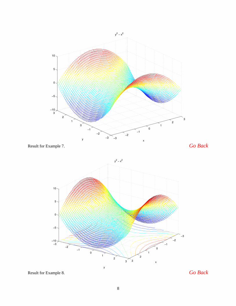
Themesh functions represent the surface with a mesh where the four edges of each mesh element are coloredaccording to the height of the function, but the faces of the mesh elements are left uncolored.

>> ezmesh(’yˆ2 - xˆ2’, [-3 3],[-3 3]); (Ex 7) See Results

The functionezmeshc also includes the level contours of the functionf (x, y) plotted on the “floor” of the3-D plot. That is, if the plotting limits in thez-direction arezmin ≤ z≤ zmax, then the level curves are plottedin the planez= zmin.

Thehidden command controls whether or not to show hidden lines (this only applies tomesh plots). Usehidden off to make hidden lines visible.

The viewing angle for 3-D graphics can be changed by dragging the mouse inside the figure window ifrotate3d has been turned on, either from the menu bar or by typingrotate3d on from the commandline. From the command line,view(125,30) will set the viewing angle with horizontal rotation 125◦ andvertical elevation 30◦. This is very similar to the viewing perspective typically used in Stewart’s text.

>> ezmeshc(’yˆ2 - xˆ2’, [-3 3],[-3 3]);>> hidden off>> view(125, 30); (Ex 8) See Results

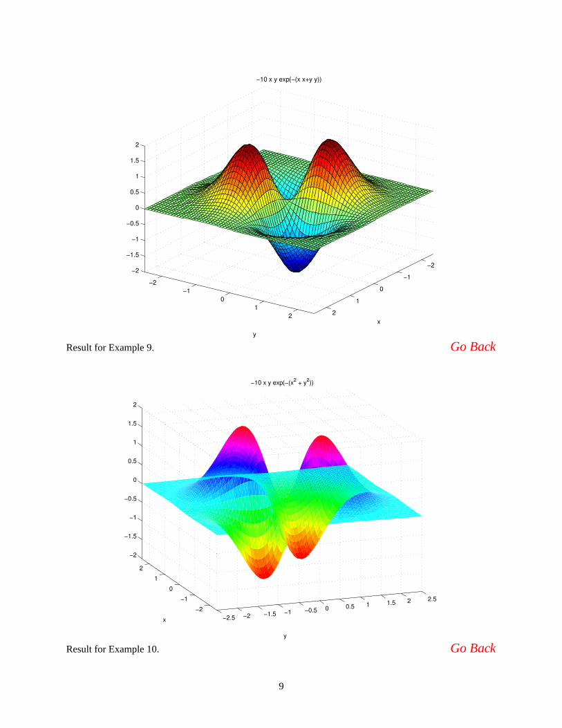
Thesurf commands produce a colored surface with the faces of each mesh element colored according tothe height of the surfacez= f (x, y).

>> ezsurf(’-10*x*y*exp(-(x*x+y*y))’, [-2.5 2.5], [-2.5 2.5]);>> view(125, 30) (Ex 9) See Results

The choice of colors for surface plots is determined by the currentcolormap. To see a list of availablecolormaps and a one-line description of each, runhelpwin graph3d . The default colormap isjet.

The shading command controls the color shading of the mesh elements making up a surface. There arethree choices:flat uses a single color within each mesh element;facetedusesflat shading with superimposedblack mesh lines (this is the default);interp uses linear interpolation to make the shading change smoothlyacross the surface.

>> ezsurf(’-10*x*y*exp(-(xˆ2 + yˆ2))’, [-2.5 2.5], [-2.5 2.5]);>> colormap(hsv)>> shading(’flat’)>> view(110,-20) (Ex 10) See Results

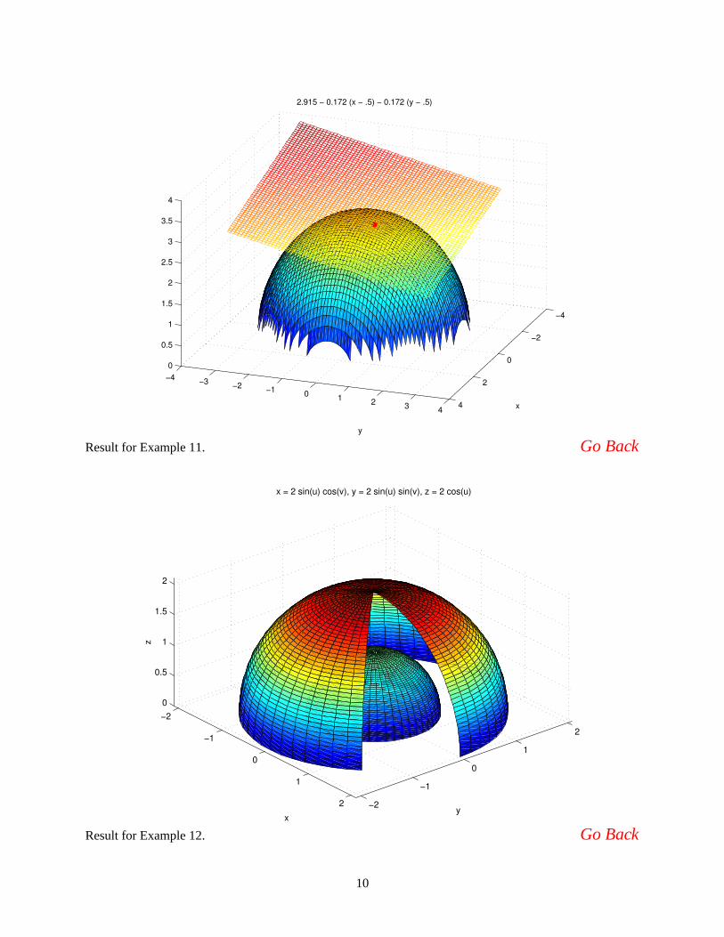
The following example graphs the upper half of the spherex2+ y2+ z2= 9 and overlays the tangent plane

at (x, y, z) = (0.5,0.5,2.915).

>> ezsurf(’sqrt(9 - xˆ2 - yˆ2)’, [-4 4], [-4 4]);>> view(110,30);>> hold on>> ezmesh(’2.915 - 0.172*(x - .5) - 0.172*(y - .5)’, [-3 3], [-3 3]);>> hidden off>> hp = plot3(.5, .5, 2.915, ’r.’);>> set(hp, ’markersize’, 20);>> axis([-4 4 -4 4 0 4]); (Ex 11) See Results

3

Parametric surfaces: ezmesh , ezsurf

[ See Section 10.5 of Stewart’s text for an introduction to parametric surfaces. ]

In the previous example for the upper half-sphere, note the ragged edge where the sphere meets thexy-plane.Here is an example of a surface that is best represented in parametric form,

x = f (u, v), y = g(u, v) z= h(u, v) for a ≤ u ≤ b, c ≤ v ≤ d.

The functionsezmesh and ezsurf accept parametric representations; in this case the first three inputarguments are the MATLAB expressions forx(u, v), y(u, v), andz(u, v). In this first example, we graph theupper halves of two concentric spheres with a section removed from the outer sphere.

>> ezsurf(’sin(u)*cos(v)’, ’sin(u)*sin(v)’,...>> ’cos(u)’, [0 pi/2 0 2*pi]);>> hold on>> ezsurf(’2*sin(u)*cos(v)’, ’2*sin(u)*sin(v)’,...>> ’2*cos(u)’, [0 pi/2 0 7*pi/4]);>> axis([-2.1 2.1 -2.1 2.1 0 2.1]);>> set(gca, ’DataAspectRatio’, [1 1 1]);>> view(50,25); (Ex 12) See Results

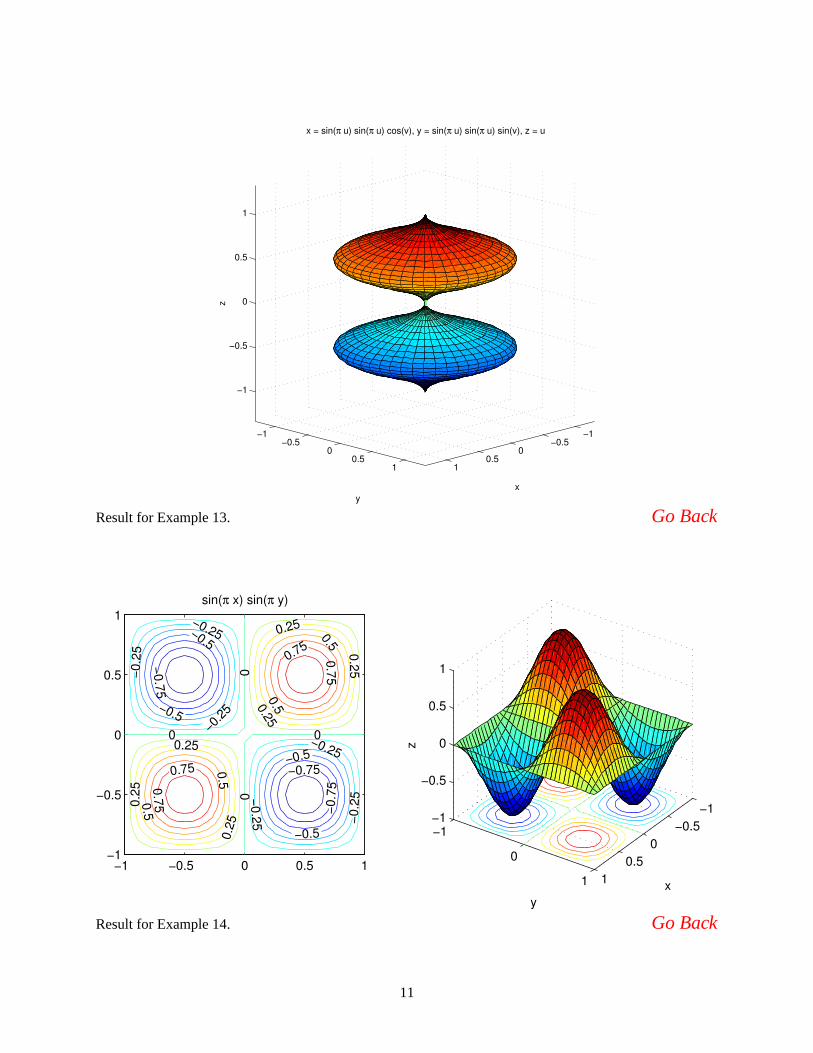
Surfaces of revolution are best represented in parametric form. In the following example, the curvex =sin2(πx) is rotated about thez-axis on the interval−1≤ z≤ 1.

>> ezsurf(’sin(pi*u)*sin(pi*u)*cos(v)’,...>> ’sin(pi*u)*sin(pi*u)*sin(v)’, ’u’, [-1 1 0 2*pi]);>> set(gca, ’DataAspectRatio’, [1 1 1]);>> view(135,15); (Ex 13) See Results

An example usingcontour and surf

To achieve better control over the graphics output, it is best to work directly with the more primitive functions,plot , plot3 , contour , mesh, surf ,…In this case the user must first create the data sets needed for plotting.This final example represents the functionz = sin(πx) sin(πx) both as a family of contour plots and as asurface using the matlab functionsurfc . The example shows how one can add labels to the contours usingtheclabel function, and also illustrates how to combine multiple plots into a single graphics window usingthesubplot function.

>> x = [-1 : 1/16 : 1];>> y = [-1 : 1/16 : 1];>> [x2,y2] = meshgrid(x,y);>> z = sin(pi*x2) .* sin(pi*y2);>> subplot(1,2,1);>> [c,h] = contour(x, y, z, [-1 : 0.125 : 1]);>> clabel(c, h, [-1 : .25 : 1]);>> set(gca, ’DataAspectRatio’, [1 1 1]);>> title(’sin(\pi x) sin(\pi y)’);>> subplot(1,2,2);>> surfc(x, y, z);>> view(125,30);>> xlabel(’x’); ylabel(’y’); zlabel(’z’);>> set(gca, ’DataAspectRatio’, [1 1 1]); (Ex 14) See Results

4

0 1 2 3 4 5 6 7 8 9 10

0

2

4

6

8

10

12

x

x + 2 sin(2 x)

Result for Example 1. Go Back

−1 0 1 2 3 4 5−4

−3

−2

−1

0

1

2

3

4

5

6

x

x

Result for Example 2. Go Back

5

−10 −5 0 5 10

−10

−8

−6

−4

−2

0

2

4

6

8

10

x

y

x = t + 2 sin(2 t), y = t + 2 cos(5 t)

Result for Example 3. Go Back

−1

−0.5

0

0.5

1

−1

−0.5

0

0.5

1−1

−0.5

0

0.5

1

x

x = cos(t), y = sin(t), z = sin(5 t)

y

z

Result for Example 4. Go Back

6

−8

−6

−4

−2

0

2

4

6

8

−3 −2 −1 0 1 2 3−3

−2

−1

0

1

2

3

x

y

y2 − x2

Result for Example 5. Go Back

−3 −2 −1 0 1 2 3−3

−2

−1

0

1

2

3

x

y

y2 − x2 − 4 = 0

z=4

z=4

z=2

z=2

z=−4 z=−4z=−2 z=−2

z=0

Result for Example 6. Go Back

7

−3−2

−10

12

3

−3−2

−10

12

3−10

−5

0

5

10

x

y2 − x2

y

Result for Example 7. Go Back

−3−2

−10

12

3

−3−2

−10

12

3

−10

−5

0

5

10

x

y2 − x2

y

Result for Example 8. Go Back

8

−2

−1

0

1

2

−2−1

01

2

−2

−1.5

−1

−0.5

0

0.5

1

1.5

2

x

−10 x y exp(−(x x+y y))

y

Result for Example 9. Go Back

−2

−1

0

1

2

−2.5 −2 −1.5 −1 −0.5 0 0.5 1 1.5 2 2.5

−2

−1.5

−1

−0.5

0

0.5

1

1.5

2

y

−10 x y exp(−(x2 + y2))

x

Result for Example 10. Go Back

9

−4

−2

0

2

4

−4 −3 −2 −1 0 1 2 3 4

0

0.5

1

1.5

2

2.5

3

3.5

4

x

2.915 − 0.172 (x − .5) − 0.172 (y − .5)

y

Result for Example 11. Go Back

−2

−1

0

1

2 −2

−1

0

1

2

0

0.5

1

1.5

2

y

x = 2 sin(u) cos(v), y = 2 sin(u) sin(v), z = 2 cos(u)

x

z

Result for Example 12. Go Back

10

−1−0.5

00.5

1

−1−0.5

00.5

1

−1

−0.5

0

0.5

1

x

x = sin(π u) sin(π u) cos(v), y = sin(π u) sin(π u) sin(v), z = u

y

z

Result for Example 13. Go Back

−1 −0.5 0 0.5 1−1

−0.5

0

0.5

1sin(π x) sin(π y)

−0.75

−0.75

−0.7

5

−0.5

−0.5

−0.5

−0.5

−0.2

5

−0.25

−0.25

−0.25

−0.25 −0.2

5

0

0

0

00.25

0.25

0.25

0.25

0.25

0.25

0.5

0.5

0.5

0.5

0.75

0.75

0.75

0.75

−1−0.5

00.5

1

−1

0

1

−1

−0.5

0

0.5

1

xy

z

Result for Example 14. Go Back

11