Matias D. Cattaneo University of Michigan July 30, 2015 D. Cattaneo University of Michigan July 30, 2015 Overview Main goal: learn about treatment e⁄ect of policy or intervention.

Regression Discontinuity Designs in Stata

Matias D. Cattaneo

University of Michigan

July 30, 2015

Overview

Main goal: learn about treatment effect of policy or intervention.

If treatment randomization available, easy to estimate treatment effects.

If treatment randomization not available, turn to observational studies.

I Instrumental variables.

I Selection on observables.

Regression discontinuity (RD) designs.

I Simple and ob jective. Requires little information, if design available.

I Might be viewed as a “local” randomized trial.

I Easy to falsify, easy to interpret.

I Careful: very local!

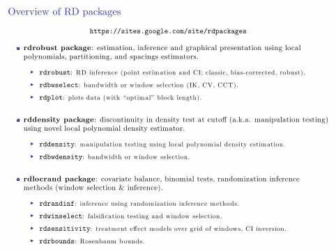
Overview of RD packages

https://sites.google.com/site/rdpackages

rdrobust package: estimation, inference and graphical presentation using localpolynomials, partitioning, and spacings estimators.

I rdrobust: RD inference (point estimation and CI; classic, bias-corrected, robust).

I rdbwselect: bandwidth or window selection (IK, CV, CCT).

I rdplot: plots data (with “optimal” block length).

rddensity package: discontinuity in density test at cutoff (a.k.a. manipulation testing)using novel local polynomial density estimator.

I rddensity: manipulation testing using local polynomial density estimation.

I rdbwdensity: bandwidth or window selection.

rdlocrand package: covariate balance, binomial tests, randomization inferencemethods (window selection & inference).

I rdrandinf: inference using randomization inference methods.

I rdwinselect: falsification testing and window selection.

I rdsensitivity: treatment effect models over grid of windows, CI inversion.

I rdrbounds: Rosenbaum bounds.

Randomized Control Trials

Notation: (Yi(0), Yi(1), Xi), i = 1, 2, . . . , n.

Treatment: Ti ∈ {0, 1}, Ti independent of (Yi(0), Yi(1), Xi).

Data: (Yi, Ti, Xi), i = 1, 2, . . . , n, with

Yi =

{Yi(0) if Ti = 0

Yi(1) if Ti = 1

Average Treatment Effect:

τATE = E[Yi(1)− Yi(0)] = E[Yi|T = 1]− E[Yi|T = 0]

Experimental Design.

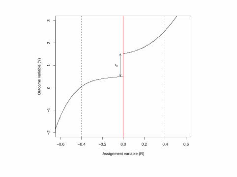
Sharp RD design

Notation: (Yi(0), Yi(1), Xi), i = 1, 2, . . . , n, Xi continuous

Treatment: Ti ∈ {0, 1}, Ti = 1(Xi ≥ x).

Data: (Yi, Ti, Xi), i = 1, 2, . . . , n, with

Yi =

{Yi(0) if Ti = 0

Yi(1) if Ti = 1

Average Treatment Effect at the cutoff:

τSRD = E[Yi(1)− Yi(0)|Xi = x] = limx↓x

E[Yi|Xi = x]− limx↑x

E[Yi|Xi = x]

Quasi-Experimental Design: “local randomization” (more later)

−0.6 −0.4 −0.2 0.0 0.2 0.4 0.6

−2

−1

01

23

Assignment variable (R)

Out

com

e va

riabl

e (Y

)

τ0

−0.6 −0.4 −0.2 0.0 0.2 0.4 0.6

−2

−1

01

23

Assignment variable (R)

Out

com

e va

riabl

e (Y

)

τ0

−0.6 −0.4 −0.2 0.0 0.2 0.4 0.6

−2

−1

01

23

Assignment variable (R)

Out

com

e va

riabl

e (Y

)

τ0

−0.6 −0.4 −0.2 0.0 0.2 0.4 0.6

−6

−4

−2

02

46

Assignment variable (R)

Out

com

e va

riabl

e (Y

)

Local Random Assignment

τ0

Empirical Illustration: Cattaneo, Frandsen & Titiunik (2015, JCI)

Problem: incumbency advantage (U.S. senate).

Data:

Yi = election outcome.

Ti = whether incumbent.

Xi = vote share previous election (x = 0).

Zi = covariates (demvoteshlag1, demvoteshlag2, dopen, etc.).

Potential outcomes:

Yi(0) = election outcome if had not been incumbent.

Yi(1) = election outcome if had been incumbent.

Causal Inference:

Yi(0) 6= Yi|Ti = 0 and Yi(1) 6= Yi|Ti = 1

Graphical and Falsification Methods

Always plot data: main advantage of RD designs!

Plot regression functions to assess treatment effect and validity.

Plot density of Xi for assessing validity; test for continuity at cutoff and elsewhere.

Important: use also estimators that do not “smooth-out”data.

RD Plots (Calonico, Cattaneo & Titiunik, JASA):

I Two ingredients: (i) Smoothed global polynomial fit & (ii) binned discontinuouslocal-means fit.

I Two goals: (i) detention of discontinuities, & (ii) representation of variability.

I Two tuning parameters:

F Global p olynom ial degree (kn).

F Location (ES or QS) and number of b ins (Jn).

Manipulation Tests & Covariate Balance and Placebo Tests

Density tests near cutoff:

I Idea: distribution of running variable should be similar at either side of cutoff.

I Method 1: Histograms & Binomial count test.

I Method 2: Density Estimator at boundary.

F Pre-b inned lo cal p olynom ial m ethod — McCrary (2008).

F New tuning-param eter-free m ethod — Cattaneo, Jansson and Ma (2015) .

Placebo tests on pre-determined/exogenous covariates.

I Idea: zero RD treatment effect for pre-determined/exogenous covariates.

I Methods: global polynomial, local polynomial, randomization-based.

Placebo tests on outcomes.

I Idea: zero RD treatment effect for outcome at values other than cutoff.

I Methods: global polynomial, local polynomial, randomization-based.

Estimation and Inference Methods

Global polynomial approach (not recommended).

Robust local polynomial inference methods.

I Bandwidth selection.

I Bias-correction.

I Confidence intervals.

Local randomization and randomization inference methods.

I Window selection.

I Estimation and Inference methods.

I Falsification, sensitivity and related methods

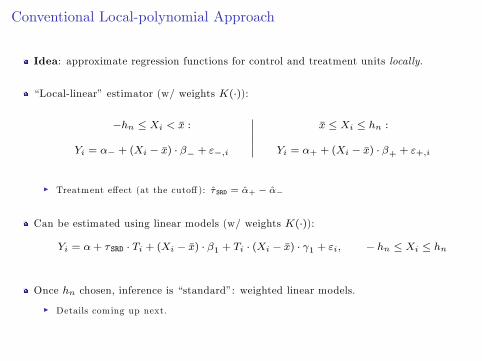
Conventional Local-polynomial Approach

Idea: approximate regression functions for control and treatment units locally.

“Local-linear” estimator (w/ weights K(·)):

−hn ≤ Xi < x : x ≤ Xi ≤ hn :

Yi = α− + (Xi − x) · β− + ε−,i Yi = α+ + (Xi − x) · β+ + ε+,i

I Treatment effect (at the cutoff): τ SRD = α+ − α−

Can be estimated using linear models (w/ weights K(·)):

Yi = α+ τSRD · Ti + (Xi − x) · β1 + Ti · (Xi − x) · γ1 + εi, − hn ≤ Xi ≤ hn

Once hn chosen, inference is “standard”: weighted linear models.

I Details coming up next.

Conventional Local-polynomial Approach

How to choose hn?

Imbens & Kalyanaraman (2012, ReStud): “optimal”plug-in,

hIK = CIK · n−1/5

Calonico, Cattaneo & Titiunik (2014, ECMA): refinement of IK

hCCT = CCCT · n−1/5

Ludwig & Miller (2007, QJE): cross-validation,

hCV = arg minh

n∑i=1

w(Xi) (Yi − µ1(Xi, h))2

Key idea: trade-off bias and variance of τSRD(hn). Heuristically:

↑ Bias(τSRD) =⇒ ↓ h and ↑ Var(τSRD) =⇒ ↑ h

Local-Polynomial Methods: Bandwidth SelectionTwo main methods: plug-in & cross-validation. Both MSE-optimal in some sense.

Imbens & Kalyanaraman (2012, ReStud): propose MSE-optimal rule,

hMSE = C1/5MSE · n

−1/5 CMSE = C(K) · Var(τSRD)Bias(τSRD)2

I IK implementation: first-generation plug-in rule.

I CCT implementation: second-generation plug-in rule.

I They differ in the way Var(τ SRD) and Bias(τ SRD) are estimated.

Imbens & Kalyanaraman (2012, ReStud): discuss cross-validation approach,

hCV = arg minh>0

CVδ (h) , CVδ (h) =n∑i=1

1(X−,[δ] ≤ Xi ≤ X+,[δ]) (Yi − µ(Xi;h))2 ,

whereI µ+,p(x;h) and µ−,p(x;h) are local polynomials estimates.

I δ ∈ (0, 1), X−,[δ] and X+,[δ] denote δ-th quantile of {Xi : Xi < x} and {Xi : Xi ≥ x}.I Our implementation uses δ = 0.5; but this is a tuning parameter!

Conventional Approach to RD

“Local-linear” estimator (w/ weights K(·)):

−hn ≤ Xi < x : x ≤ Xi ≤ hn :

Yi = α− + (Xi − x) · β− + ε−,i Yi = α+ + (Xi − x) · β+ + ε+,i

I Treatment effect (at the cutoff): τ SRD = α+ − α−

Construct usual t-test. For H0 : τSRD = 0,

T (hn) =τSRD√Vn

=α+ − α−√V+,n + V−,n

≈d N (0, 1)

95% Confidence interval:

I(hn) =

[τSRD ± 1.96 ·

√Vn

]

Bias-Correction Approach to RD

Note well: for usual t-test,

T (hMSE) =τSRD√Vn≈d N (B, 1) 6= N (0, 1), B > 0

I Bias B in RD estimator captures “curvature” of regression functions.

Undersmoothing/“Small Bias”Approach: Choose “smaller”hn... Perhaps hn = 0.5 · hIK?

=⇒ Not clear guidance & power loss!

Bias-correction Approach:

T bc(hn, bn) =τSRD − Bn√

Vn≈d N (0, 1)

=⇒ 95% Confidence Interval: Ibc(hn, bn) =[ (

τSRD − Bn)± 1.96 ·

√Vn

]

How to choose bn? Same ideas as before... bn = C · n−1/7

Robust Bias-Correction Approach to RDRecall:

T (hn) =τSRD√Vn≈d N (0, 1) and T

bc(hn, bn) =

τSRD − Bn√Vn

≈d N (0, 1)

I Bn is constructed to estimate leading bias B.

Robust approach:

T bc(hn, bn) =τSRD − Bn√

Vn=τSRD − Bn√

Vn︸ ︷︷ ︸≈d N (0,1)

+Bn − Bn√

Vn︸ ︷︷ ︸≈d N (0,γ)

Robust bias-corrected t-test:

T rbc(hn, bn) =τSRD − Bn√Vn + Wn

=τSRD − Bn√

Vbcn

≈d N (0, 1)

=⇒ 95% Confidence Interval:

Irbc(hn, bn) =

[ (τSRD − Bn

)± 1.96 ·

√Vbcn

], Vbcn = Vn + Wn

Local-Polynomial Methods: Robust Inference

Approach 1: Undersmoothing/“Small Bias”.

I(hn) =

[τSRD ± 1.96 ·

√Vn

]

Approach 2: Bias correction (not recommended).

Ibc(hn, bn) =

[ (τSRD − Bn

)± 1.96 ·

√Vn

]

Approach 3: Robust Bias correction.

Irbc(hn, bn) =

[ (τSRD − Bn

)± 1.96 ·

√Vn + Wn

]

Local-randomization approach and finite-sample inference

Popular approach: local-polynomial methods.

I Approximates regression function and relies on continuity assumptions.

I Requires: choosing weights, bandwidth and polynomial order.

Alternative approach: local-randomization + randomization-inference

I Gives an alternative that can be used as a robustness check.

I Key assumption: exists window W = [−hn, hn] around cutoff (−hn < x < hn) where

Ti independent of (Yi(0), Yi(1)) (for all Xi ∈ W )

I In words: treatment is randomly assigned within W .

I Good news: if plausible, then RCT ideas/methods apply.

I Not-so-good news: most plausible for very small windows (very few observations).

I One solution: employ small window but use randomization-inference methods.

I Requires: choosing randomization rule, window and statistic.

Local-randomization approach and finite-sample inference

Recall key assumption: exists W = [−hn, hn] around cutoff (−hn < x < hn) where

Ti independent of (Yi(0), Yi(1)) (for all Xi ∈W )

How to choose window?

I Use balance tests on pre-determined/exogenous covariates.

I Very intuitive, easy to implement.

How to conduct inference? Use randomization-inference methods.

1 Choose statistic of interest. E.g., t-stat for difference-in-means.

2 Choose randomization rule. E.g., number of treatments and controls given.

3 Compute finite-sample distribution of statistics by permuting treatment assignments.

Local-randomization approach and finite-sample inference

Do not forget to validate & falsify the empirical strategy.

1 Plot data to make sure local-randomization is plausible.

2 Conduct placebo tests.

(e.g., use pre-intervention outcomes or other covariates not used select W )

3 Do sensitivity analysis.

See Cattaneo, Frandsen and Titiunik (2015) for introduction.

See Cattaneo, Titiunik and Vazquez-Bare (2015) for further results andimplementation.