G. H. Patel College of Engineering & Technology Branch : Information Technology Name Of Subject : Numerical Methods For Computer Engineering Subject Code : 2710210 Name Of Unit : Ordinary differential equations Topic : Euler’s method and Runge-Kutta methods • Guided By : Prof. Krupal Parikh • Submitted By : Mira Y Patel

Welcome message from author
This document is posted to help you gain knowledge. Please leave a comment to let me know what you think about it! Share it to your friends and learn new things together.
Transcript

G. H. Patel College of Engineering & Technology
Branch : Information Technology
Name Of Subject : Numerical Methods For Computer Engineering
Subject Code : 2710210
Name Of Unit : Ordinary differential equations
Topic : Euler’s method and Runge-Kutta methods
• Guided By : Prof. Krupal Parikh
• Submitted By : Mira Y Patel (140110723006)

Euler’s Method Derivation of Euler’s method :
At x = 0, we are given the value of y = y₀. Let us
call x = 0 as x₀. Now since we know the slope of y
with respect to x, that is, f(x,y) , then at x =x₀, the
slope is f(x₀,y₀). Both x₀ and y₀ are known from the
initial condition y(x₀) = y₀.

Euler’s Method Derivation of Euler’s method :
Φ
Step size, h
x
y
x0,y0
True value
y1,
Predictedvalue
00,, yyyxfdx
dy
Run
Rise
01
01
xx
yy
00 , yxf
010001 , xxyxfyy
hyxfy 000 ,
Slope
Figure 1 Graphical interpretation of the first step of Euler’s method

Euler’s Method Derivation of Euler’s method :
Φ
Step size
h
True Value
yi+1, Predicted value
yi
x
y
xi xi+1
hyxfyy iiii ,1
ii xxh 1
This formula is known as
Euler’s method and is
illustrated graphically in
Figure 2.
In some books, it is also
called the Euler-Cauchy
method.
Figure 2. General graphical interpretation of Euler’s method
Euler’s Method Modified Euler’s method :
A fundamental source of error in Euler’s method is that the derivative
at the beginning of the interval is assumed to apply across the entire
interval.
Two simple modifications are available to circumvent this shortcoming:
o Heun’s Method
o The Midpoint (or Improved Polygon) Method
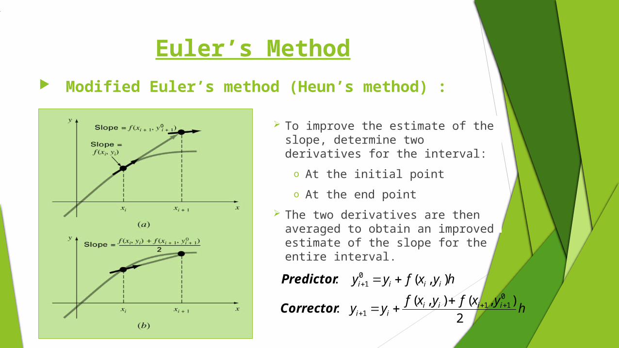
Euler’s Method Modified Euler’s method (Heun’s method) :
To improve the estimate of the slope, determine two derivatives for the interval:
o At the initial point
o At the end point
The two derivatives are then averaged to obtain an improved estimate of the slope for the entire interval.
hyxfyxf
yy
hyxfyy
iiiiii
iiii
2
),(),(:
),( :0
111
01
Corrector
Predictor
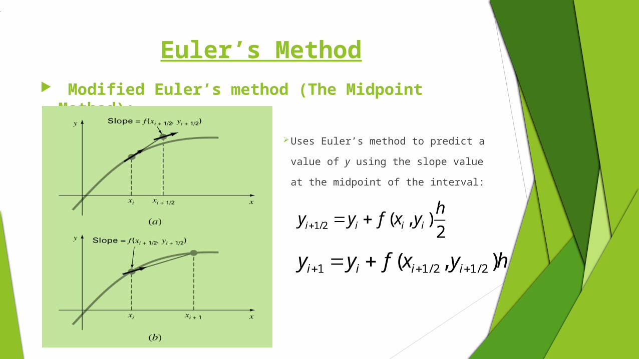
Euler’s Method Modified Euler’s method (The Midpoint
Method):
Uses Euler’s method to predict a
value of y using the slope value
at the midpoint of the interval:
1/2 ( , )2i i i i
hy y f x y
hyxfyy iiii ),( 2/12/11

Euler’s Method Error analysis for Euler’s method :
o Numerical solutions of ODEs involves two types of error:
Truncation error
• Local truncation error
• Propagated truncation error
The sum of the two is the total or global truncation
error
Round-off errors (due to limited digits in representing
numbers in a computer)
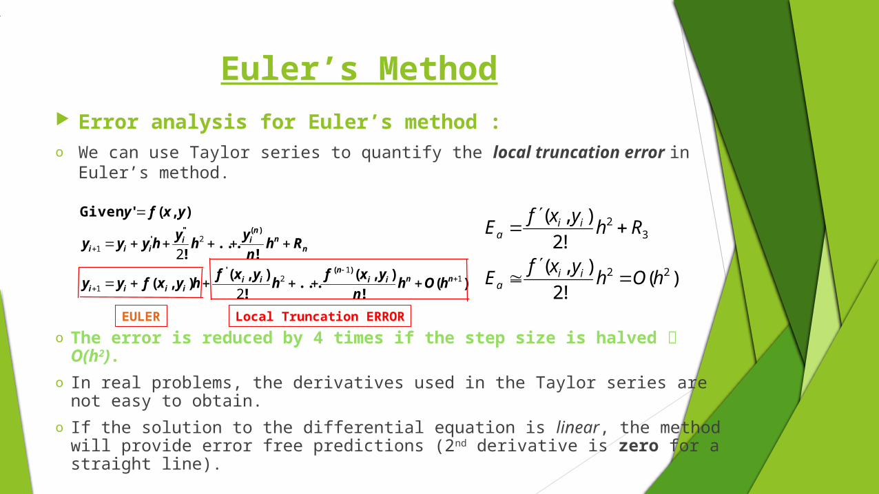
Euler’s Method Error analysis for Euler’s method :o We can use Taylor series to quantify the local truncation error in
Euler’s method.
o The error is reduced by 4 times if the step size is halved O(h2).
o In real problems, the derivatives used in the Taylor series are not easy to obtain.
o If the solution to the differential equation is linear, the method will provide error free predictions (2nd derivative is zero for a straight line).
)(!
),(...
!
),(),(
!...
!
),(' Given
)('
)("'
11
21
21
2
2
nniin
iiiiii
nn
nii
iii
hOhn
yxfh
yxfhyxfyy
Rhn
yh
yhyyy
yxfy
)(!2
),(!2
),(
22
32
hOhyxf
E
Rhyxf
E
iia
iia
EULER Local Truncation ERROR
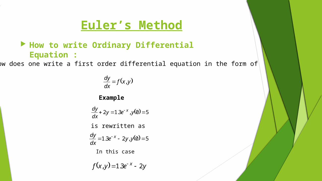
Euler’s Method How to write Ordinary Differential Equation :
How does one write a first order differential equation in the form of
yxfdx
dy,
Example
50,3.12 yeydx
dy x
is rewritten as
50,23.1 yyedx
dy x
In this case
yeyxf x 23.1,
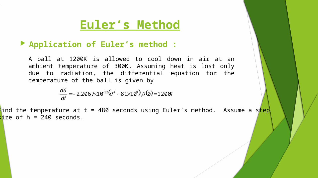
Euler’s Method Application of Euler’s method :
A ball at 1200K is allowed to cool down in air at an ambient temperature of 300K. Assuming heat is lost only due to radiation, the differential equation for the temperature of the ball is given by
Kdt
d12000,1081102067.2 8412
Find the temperature at t = 480 seconds using Euler’s method. Assume a step size of h = 240 seconds.

Euler’s Method Application of Euler’s method : Solution step 1:
8412 1081102067.2
dt
d
8412 1081102067.2, tf
K
f
htf
htf iiii
09.106
2405579.41200
24010811200102067.21200
2401200,01200
,
,
8412
0001
1
1 is the approximate temperature at 240240001 httt
K09.106240 1

Euler’s Method Application of Euler’s method : Solution step 2:
For 09.106,240,1 11 ti
K
f
htf
32.110
240017595.009.106
240108109.106102067.209.106
24009.106,24009.106
,
8412
1112
2 is the approximate temperature at 48024024012 httt
K32.110480 2

Runge-Kutta Methods Runge-Kutta (RK) methods achieve the accuracy of a Taylor
series approach without requiring the calculation of higher derivatives.
),(
),,(
1
2211
1
ii
nn
iiii
yxfk
kakaka
hhyxyy
constants are s
FunctionIncrement
'a
),(
),(
),(
11,122,1111
22212133
11112
hkqhkqhkqyhpxfk
hkqhkqyhpxfk
hkqyhpxfk
nnnnninin
ii
ii
constants are s’ and s’ q p
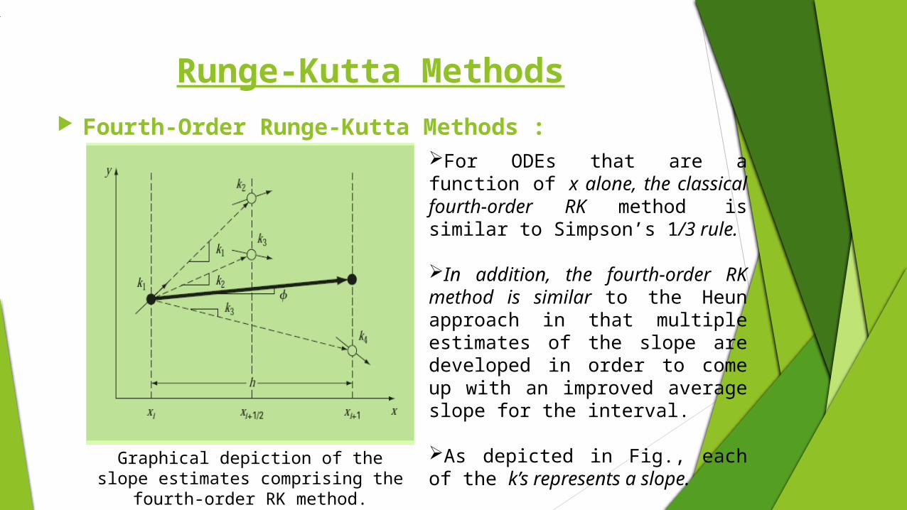
Runge-Kutta Methods Fourth-Order Runge-Kutta Methods :
For ODEs that are a function of x alone, the classical fourth-order RK method is similar to Simpson’s 1/3 rule.
In addition, the fourth-order RK method is similar to the Heun approach in that multiple estimates of the slope are developed in order to come up with an improved average slope for the interval.
As depicted in Fig., each of the k’s represents a slope.
Graphical depiction of the slope estimates comprising the fourth-
order RK method.

Runge-Kutta Methods Fourth-Order Runge-Kutta Methods :
For 0)0(),,( yyyxfdx
dy
Runge-Kutta 4th order method is given by
hkkkkyy ii 43211 226
1
where
ii yxfk ,1
hkyhxfk ii 12 2
1,
2
1
hkyhxfk ii 23 2
1,
2
1
hkyhxfk ii 34 ,
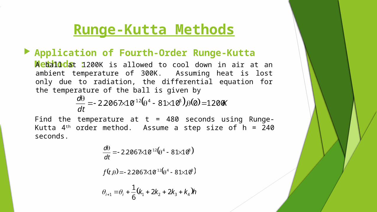
Runge-Kutta Methods Application of Fourth-Order Runge-Kutta
Methods :A ball at 1200K is allowed to cool down in air at an ambient temperature of 300K. Assuming heat is lost only due to radiation, the differential equation for the temperature of the ball is given by
Kdt
d12000,1081102067.2 8412
Find the temperature at t = 480 seconds using Runge-Kutta 4th order method. Assume a step size of h = 240 seconds.
8412 1081102067.2
dt
d
8412 1081102067.2, tf
hkkkkii 43211 226
1
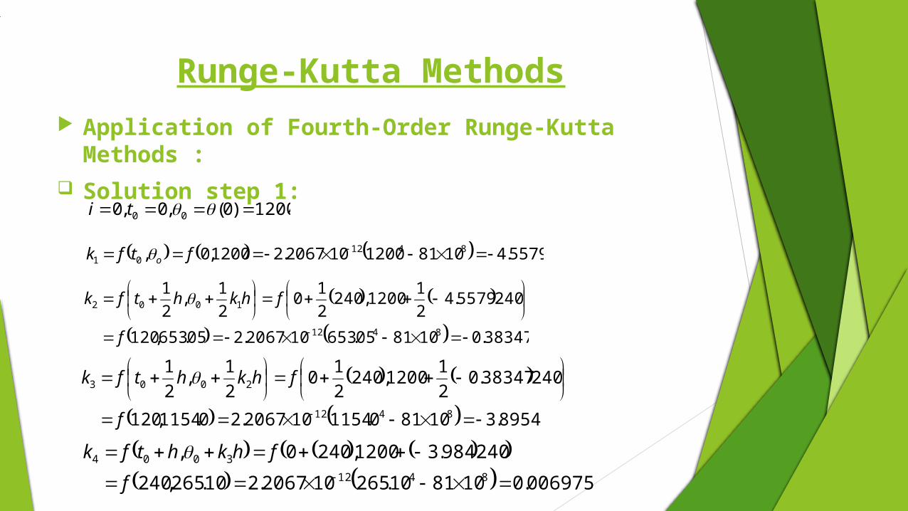
Runge-Kutta Methods Application of Fourth-Order Runge-Kutta
Methods : Solution step 1:
1200)0(,0,0 00 ti
5579.410811200102067.21200,0, 841201 ftfk o
38347.0108105.653102067.205.653,120
2405579.42
11200,240
2
10
2
1,
2
1
8412
1002
f
fhkhtfk
8954.310810.1154102067.20.1154,120
24038347.02
11200,240
2
10
2
1,
2
1
8412
2003
f
fhkhtfk
0069750.0108110.265102067.210.265,240
240984.31200,2400,8412
3004
f
fhkhtfk
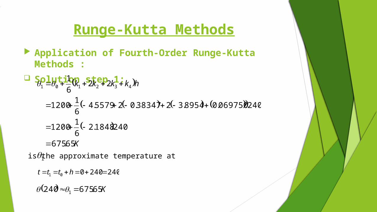
Runge-Kutta Methods Application of Fourth-Order Runge-Kutta
Methods : Solution step 1:
K
hkkkk
65.675
2401848.26
11200
240069750.08954.3238347.025579.46
11200
226
1432101
1is the approximate temperature at
240240001 httt
K65.675240 1

Runge-Kutta Methods Application of Fourth-Order Runge-Kutta
Methods : Solution step 2:Kti 65.675,240,1 11
44199.0108165.675102067.265.675,240, 8412111 ftfk
31372.0108161.622102067.261.622,360
24044199.02
165.675,240
2
1240
2
1,
2
1
8412
1112
f
fhkhtfk
34775.0108100.638102067.200.638,360
24031372.02
165.675,240
2
1240
2
1,
2
1
8412
2113
f
fhkhtfk
25351.0108119.592102067.219.592,480
24034775.065.675,240240,8412
3114
f
fhkhtfk

Runge-Kutta Methods Application of Fourth-Order Runge-Kutta
Methods : Solution step 2:
K
hkkkk
91.594
2400184.26
165.675
24025351.034775.0231372.0244199.06
165.675
226
1432112
q2 is the approximate temperature at
48024024012 htt
K91.594480 2

Comparison of Euler's Method and Runge-Kutta Methods
0
200
400
600
800
1000
1200
1400
0 100 200 300 400 500
Time, t(sec)
Tem
pera
ture
,θ(K
)
Exact
4th order
Heun
Euler
Figure 3. Comparison of Euler's Method and Runge-Kutta Methods

References
http://mat.iitm.ac.in
http://en.m.wikipedia.org/wiki/Euler_method
http://en.m.wikipedia.org/wiki/Runge-Kutta_methods
http://www.classzone.com
http://mathforcollege.com

Certificate
I Mira Y Patel(140110723006) assure that material which I
prepared is not plagiarized material. I Prepared it under the
guidance of subject faculty. The references are also mentioned,
which are used for the ppt.
Sign
Mira Y Patel

THANK YOU
Related Documents