Math/Phys 594: Homework 5 Solutions - Saad Qadeer

Math/Phys 594: Homework 5 Solutions

February 13, 2019

4.1.2 For θ = 1+2 cos(θ), find and classify all the fixed points and sketch the phase portraiton the circle.

Set θ = 0 to get cos(θ) = −1/2 ⇒ θ∗± = ±2π/3. Let f(θ) = 1 + 2 cos(θ); then,

f ′(θ) = −2 sin(θ) ⇒ f ′(θ∗±) = ∓√

3 so we infer that θ∗+ is stable and θ∗− is unstable. Thephase portrait is shown in Figure 1.

Figure 1: Problem 4.1.2

4.1.7 For θ = sin(kθ), where k is a positive integer, find and classify all the fixed pointsand sketch the phase portrait on the circle.

Let f(θ) = sin(kθ). Then, the fixed points are given by the solution of f(θ) = 0 so thatθ∗j = j

kπ for j = 0, 1, . . . , 2k − 1 (for higher j, the fixed points start repeating). In order

to determine their stability, we compute f ′(θ) = k cos(kθ) ⇒ f ′(θ∗j ) = k cos(jπ) = k(−1)j.We conclude that {θ∗j} for odd j are stable while {θ∗j} for even j are unstable. An easy wayof visualizing this is to note that the origin is always unstable and successive fixed pointsalternate stabilities. See Figure 2 for the phase portraits for k = 3 and k = 4 (the onlymajor difference between them is the stability of the fixed point at θ = π).

1

(a) k = 3 (b) k = 4

Figure 2: Problem 4.1.7

4.1.8 (Potentials for vector fields on the circle)

(a) Consider the vector field on the circle given by θ = cos(θ). Show that this system hasa single-valued potential V (θ), i.e., for each point on the circle, there is a well-definedvalue of V such that θ = −dV/dθ. (As usual, θ and θ + 2kπ are to be regarded asthe same point on the circle, for each integer k.)

(b) Now consider θ = 1. Show that there is no single-valued potential V (θ) for this vectorfield on the circle.

(c) What’s the general rule? When does θ = f(θ) have a single-valued potential?

(a) Solving V ′(θ) = − cos(θ) gives V (θ) = sin(θ) (the constant is not important since wewant to show that at least one solution exists). Note that V (θ) is 2π–periodic so it iswell-defined on the circle.

(b) Solving V ′(θ) = −1 gives V (θ) = −θ + c (we include c here as we are looking to showno solutions exist). For V (θ) to be defined on the circle, we require V (0) = V (2π).This yields c = −2π + c ⇒ 0 = −2π, which is clearly false. We conclude that nopotential function on the circle exists for this vector field.

(c) Observe that V (θ) is well-defined on the circle if, for any θ0, we have V (θ0) = V (θ0+2π),so that

V (θ0)− V (θ0 + 2π) = 0⇒∫ θ0+2π

θ0

−V ′(θ) dθ = 0

from the Fundamental Theorem of Calculus. Since we require f(θ) = −V ′(θ), we obtain∫ θ0+2π

θ0f(θ) dθ = 0. By noting that the integral is over the circle for any choice of θ0,

we can simply reduce this to∫ 2π

0f(θ) dθ = 0. By following the chain of deductions the

other way, it can be seen that this is a sufficient condition as well.

2

4.2.1 (Church bells) The bells of two different churches are ringing. One bell rings every3 seconds, and the other rings every 4 seconds. Assume that the bells have just rung atthe same time. How long will it be until the next time they ring together? Answer thequestion in two ways: using common sense, and using the method of Example 4.2.1.

The first bell rings at t = 0, 3, 6, . . . while the second bell rings at t = 0, 4, 8, . . . so thetwo coincide at multiples of 12. In particular, the next time they chime together will be att = 12.

Alternatively, the first bell is governed by θ1 = 2π/3 and the second by θ2 = 2π/4 (sincethe angular velocities are 2π/T ). Letting φ = θ1 − θ2 be the difference between the two,we obtain φ = θ1 − θ2 = 2π/12; thus, the difference is a uniform oscillator with periodTd = 2π

2π/12= 12. In particular, if the difference is zero at t = 0, it will be the same at t = 12

again so it takes 12 seconds for the bells to ring together again.

4.2.3 (The clock problem) Here’s an old chestnut from high school algebra: at 12:00, thehour and minute hands of a clock are perfectly aligned. When is the next time they will bealigned? (Solve the problem by the methods of this section, and also by some alternativeapproach of your choosing.)

The hour hand has a period of Th = 60 × 12 = 720 minutes so θh = 2π/720 governsits motion. Similarly, the minute hand has a period of Tm = 60 minutes so θm = 2π/60describes it. Letting φ = θm− θh be the difference, we obtain φ = 2π(11/720); the differencehas a period of Td = 720/11 minutes so the two hands coincide again 65.4545... minutes after12 ⇒ at 1:05:27.27...

Alternatively, note that before one hour has elapsed, the two hands cannot coincide. At1:00, the minute hand is vertical while the hour hand is pointing towards 1, so it makes a30◦ angle with the minute hand. Each minute, the minute hand traverses 6◦ while the hourhand gains 0.5◦. As a result, m minutes after 1:00, the minute hand makes an angle of 6m◦

while the hour hand makes an angle of (30 + 0.5m)◦. Setting the two equal to each othergives

6m = 30 + 0.5m⇒ 5.5m = 30⇒ m = 60/11 ≈ 5.45 . . .

which is the same result as earlier.

4.3.4 For θ = sin(θ)µ+cos(θ)

, draw the phase portrait as functions of the control parameter µ.Classify the bifurcations that occur as µ varies, and find all the bifurcation values of µ.

The phase portraits on the line and circle are shown in Figure 3. This is a slightly weirdproblem in the sense that, for certain values of µ, the problem is not well-posed. If we glossover that and treat the singularities (i.e. values of θ at which the denominator µ+ cos(θ) iszero) in the same manner as fixed points, we obtain pretty familiar behavior. Note that a pairof stable singularities is produced at the origin as µ is increased past −1. This coincides withthe fixed point at zero switching from stable to unstable, so we can say that a supercriticalpitchfork bifurcation occurs at µ = −1. Similar behavior occurs at µ = 1.

3

(a) µ < −1

(b) µ = −1

(c) −1 < µ < 1

(d) µ = 1

(e) µ > 1

Figure 3: Problem 4.3.4: Singularities represented by ×.

4

4.3.5 For θ = µ + cos(θ) + cos(2θ), draw the phase portrait as functions of the controlparameter µ. Classify the bifurcations that occur as µ varies, and find all the bifurcationvalues of µ.

In order to analyze this, we rewrite the problem as θ = (cos(θ)+cos(2θ))−(−µ) and sketchthe two curves on the same axes. To draw the first one, it helps to use the trigonometricidentity

cos(A) + cos(B) = 2 cos

(A+B

2

)cos

(A−B

2

)to obtain

g(θ) := cos(θ) + cos(2θ) = 2 cos

(3θ

2

)cos

(θ

2

).

This form allows us to sketch the graph of g(θ) easily by finding the zeros of the individualcomponents and figuring out the signs in between. This yields the curve shown in Figure 4.

Figure 4: Problem 4.3.5 (drawn over [0, 4π] for better visualization)

We will clearly have many saddle-node bifurcations as the horizontal line at height −µbecomes tangent to g(θ). The local maxima clearly occur at heights 2 (corresponding toθ = 2kπ) and 0 (for θ = (2k + 1)π). For the local minima, we differentiate g(θ) and set itequal to zero:

g′(θ) = − sin(θ)− 2 sin(2θ) = 0⇒ sin(θ)(4 cos(θ) + 1) = 0

which yields sin(θ) = 0 ⇒ θ = kπ (which we already know about) and cos(θ) = −1/4.Denote any solution of this by θ; then,

g(θ) = cos(θ) + (2 cos2(θ)− 1) = −9/8.

We conclude that saddle-node bifurcations occur at µ = −2, µ = 0 and µ = 9/8. Thephase portraits on the circle are shown in Figure 5.

5

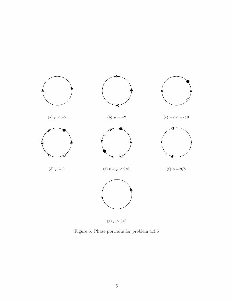
(a) µ < −2 (b) µ = −2 (c) −2 < µ < 0

(d) µ = 0 (e) 0 < µ < 9/8 (f) µ = 9/8

(g) µ > 9/8

Figure 5: Phase portraits for problem 4.3.5

6

4.4.4 (Torsional spring) Suppose that our overdamped pendulum is connected to a torsionalspring. As the pendulum rotates, the spring winds up and generates an opposing torque−kθ. Then the equation of motion becomes bθ +mgL sin(θ) = Γ− kθ.

(a) Does the equation give a well-defined vector field on the circle?

(b) Nondimensionalize the equation.

(c) What does the pendulum do in the long run?

(d) Show that many bifurcations occur as k is varied from 0 to ∞. What kind of bifur-cations are they?

(a) We have

θ =Γ

b− k

bθ − mgL

bsin(θ). (1)

Since the right hand side of (1) is not a 2π–periodic function, it does not represent awell-defined vector field on the circle.

(b) Let T be the time scale and define τ = t/T . This yields

1

T

dθ

dτ=

Γ

b− k

bθ − mgL

bsin(θ)⇒ dθ

dτ=TΓ

b− kT

bθ − mgLT

bsin(θ).

Setting mgLT/b = 1 (for simplicity of analysis) gives T = b/mgL. Define

α =TΓ

b=

Γ

mgL, β =

kT

b=

k

mgL

to get

dθ

dτ= α− βθ − sin(θ).

(c) Depending on the values of k and Γ (and hence α and β), this system may have zeroor multiple fixed points. These cases are shown in Figure 6. Note that, in the absenceof any fixed points, the system keeps oscillating forever. This occurs only for β = 0and |α| > 1, i.e., no torsional spring and a large external torque.

In the case of multiple fixed points, the system will approach the nearest stable fixedpoint. Note that if β < 0 (i.e., k < 0), the fixed points at the ends will be necessarilyunstable so the system could again oscillate indefinitely if the initial condition is chosenbeyond these fixed points. However, for β > 0, the system will necessarily settle downto a stable fixed point.

(d) As k is varied from 0 to ∞, the slope of the straight line goes from 0 to −∞. As aresult, pairs of fixed points that are formed by the intersection of the line and the sinecurve collide and vanish, as the line becomes steeper. These are instances of saddle-node bifurcations. (This is fairly similar to Problem 3.4.11 that we saw in an earlierhomework)

7

Figure 6: Problem 4.4.4

4.5.3 (Excitable systems) Suppose you stimulate a neuron by injecting it with a pulseof current. If the stimulus is small, nothing dramatic happens: the neuron increases itsmembrane potential slightly, and then relaxes back to its resting potential. However, if thestimulus exceeds a certain threshold, the neuron will “fire” and produce a large voltagespike before returning to rest. Surprisingly, the size of the spike doesn’t depend much onthe size of the stimulus – anything above threshold will elicit essentially the same response.Similar phenomena are found in other types of cells and even in some chemical reactions(Winfree 1980, Rinzel and Ermentrout 1989, Murray 1989). These systems are calledexcitable. The term is hard to define precisely, but roughly speaking, an excitable systemis characterized by two properties: (1) it has a unique, globally attracting rest state, and(2) a large enough stimulus can send the system on a long excursion through phase spacebefore it returns to the resting state.This exercise deals with the simplest caricature of an excitable system. Let θ = µ+ sin(θ),where µ is slightly less than 1.

(a) Show that the system satisfies the two properties mentioned above. What objectplays the role of the “rest state”? And the “threshold”?

(b) Let V (t) = cos(θ(t)). Sketch V (t) for various initial conditions. (Here, V is analogousto the neuron’s membrane potential, and the initial conditions correspond to differentperturbations from the rest state.)

(a) The phase portrait for this problem is shown in Figure 7(a). Note that there is exactlyone stable fixed point, corresponding to the unique attracting rest state. In addition,if we stimulate the system to beyond the unstable fixed point, it will cycle through theentire phase space and approach the the stable fixed point. We can then say that theunstable fixed point functions as the threshold.

(b) The plot of V (t) vs t is shown in Figure 7(b). Observe that, irrespective of the initial

8

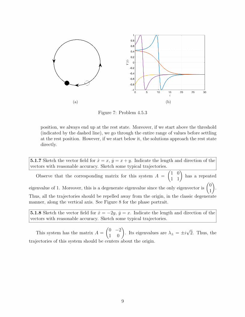
(a) (b)

Figure 7: Problem 4.5.3

position, we always end up at the rest state. Moreover, if we start above the threshold(indicated by the dashed line), we go through the entire range of values before settlingat the rest position. However, if we start below it, the solutions approach the rest statedirectly.

5.1.7 Sketch the vector field for x = x, y = x+ y. Indicate the length and direction of thevectors with reasonable accuracy. Sketch some typical trajectories.

Observe that the corresponding matrix for this system A =

(1 01 1

)has a repeated

eigenvalue of 1. Moreover, this is a degenerate eigenvalue since the only eigenvector is

(01

).

Thus, all the trajectories should be repelled away from the origin, in the classic degeneratemanner, along the vertical axis. See Figure 8 for the phase portrait.

5.1.8 Sketch the vector field for x = −2y, y = x. Indicate the length and direction of thevectors with reasonable accuracy. Sketch some typical trajectories.

This system has the matrix A =

(0 −21 0

). Its eigenvalues are λ± = ±i

√2. Thus, the

trajectories of this system should be centers about the origin.

9

Figure 8: Problem 5.1.7

Figure 9: Problem 5.1.8

10

4.3.2 (Bonus 1) The oscillation period for the nonuniform oscillator is given by the integralT =

∫ π−π

1ω−a sin(θ) dθ, where ω > a > 0. Evaluate this integral as follows:

(a) Let u = tan(θ/2). Solve for θ and express dθ in terms of u and du.

(b) Show that sin(θ) = 2u/(1 + u2).

(c) Show that u→ ±∞ as θ → ±π, and use that fact to rewrite the limits of integration.

(d) Express T as an integral with respect to u.

(e) Finally, complete the square in the denominator of the integrand of (d), and reducethe integral to the one studied in Exercise 4.3.1, for a suitable choice of x and r.

(a) We have dudθ

= 12

sec2(θ/2) = 12(1 + tan2(θ/2)) = 1

2(1 + u2)⇒ dθ = 2

1+u2du.

Alternatively, we can write θ = 2 tan−1(u) to get dθdu

= 21+u2

⇒ dθ = 21+u2

du.

(b) Note that tan(θ/2) = u implies that sin(θ/2) = u√1+u2

and cos(θ/2) = 1√1+u2

so that

sin(θ) = 2 sin(θ/2) cos(θ/2) =2u

1 + u2.

(c) Since tan(x)→ ±∞ as x→ ±π/2, we infer that u→ ±∞ as θ → ±π.

(d) We obtain

T =

∫ π

−π

1

ω − a sin(θ)dθ =

∫ ∞−∞

1

ω − a(

2u1+u2

) ( 2

1 + u2

)du.

(e) We have

T =

∫ ∞−∞

1

ω − a(

2u1+u2

) ( 2

1 + u2

)du

=2

ω

∫ ∞−∞

1

u2 − 2(aω

)u+ 1

du

=2

ω

∫ ∞−∞

1

[(u)2 − 2(aω

)(u) +

(aω

)2]−(aω

)2+ 1

du

=2

ω

∫ ∞−∞

1(u− a

ω

)2+(ω2−a2ω2

) du=

2

ω

π√ω2−a2ω2

=2π√ω2 − a2

where we used the fact that∫∞−∞

1(x−b)2+c dx = π√

cfor any b and any c > 0.

11

4.1.7 (Bonus 2)

(a) Show that r ≤ 1.

(b) Numerically solve the Kuramoto model, plot r(t) vs. t for different values of K andestimate Kc.

(a) Since

reiψ =1

N

N∑j=1

eiθj ,

taking absolute values of both sides and applying the triangle inequality gives

r = |reiψ| = 1

N

∣∣∣∣∣N∑j=1

eiθj

∣∣∣∣∣ ≤ 1

N

N∑j=1

∣∣eiθj ∣∣ = 1.

(a) K = 0.6 (b) K = 0.66

(c) K = 0.656 (d) K = 0.657

Figure 10: Plots of r(t) for various values of K. These suggest that Kc lies between 0.656and 0.657.

(b) See the attached kuramoto.m file for the code. We present the results for N = 30. Forreproducibility, we fix the natural angular velocities {ωl} and initial phases {θl(0)};these are chosen to be uniformly distributed over [0, 1] and [0, 2π) respectively. Theresults, shown in Figure 10, suggest that Kc in this case lies between 0.656 and 0.657.

12