Mathematics Primer for Introduction to Mathematical Statistics ...

Mathematics Primer for

Introduction to Mathematical Statistics

8th Edition

Joseph W. McKean

Copyright ©2017 by Joseph W. McKean at Western Michigan University.

All rights reserved.

Reproduction or translation of any part of this work beyond that permitted by Sec-tions 107 and 108 of the 1976 United States Copyright Act without the permissionof the copyright owner is unlawful.

Contents

1 Introduction 1

2 Sequences 3

2.0.1 Limits Supremum and Infimum . . . . . . . . . . . . . . . . . 42.0.2 Infinite Series . . . . . . . . . . . . . . . . . . . . . . . . . . . 6

3 Derivatives 11

4 Integration 15

4.0.3 Multiple Integration . . . . . . . . . . . . . . . . . . . . . . . 17

iii

Chapter 1

Introduction

The purpose of this appendix is to review some of the calculus concepts which areused in the text. It is not meant to be complete and readers who have difficulty withsome of these concepts are advised to consult a calculus text for more explanation.We do reference Buck’s (1965) advanced calculus book but our discussion concernsfundamental results which can be found in any calculus book.

For the most part, we state and discuss the concepts. In the section on sequences,we spend a little time on proofs since the reader may not be familiar with a few ofthe concepts such as limit supremums.

1

Chapter 2

Sequences

Let {an} be a sequence of real numbers. Recall from calculus that an → a(limn→∞ an = a) if and only if

for every ǫ > 0, there exists an N0 such that n ≥ N0 =⇒ |an − a| < ǫ. (2.0.1)

Let A be a set of real numbers which is bounded from above; that is, thereexists an M ∈ R such that x ≤ M for all x ∈ A. Recall that a is the supremum

of A if a is the least of all upper bounds of A. From calculus, we know that thesupremum of a set bounded from above exists. Furthermore, we know that a isthe supremum of A if and only if, for all ǫ > 0, there exists an x ∈ A such thata − ǫ < x ≤ a. Similarly, we can define the infimum of A. The first theorem onlimits is the Sandwich Theorem.

Theorem 2.0.1 (Sandwich Theorem). Suppose for sequences {an}, {bn}, and {cn}that cn ≤ an ≤ bn, for all n, and that limn→∞ bn = limn→∞ cn = a. Then

limn→∞ an = a.

Proof: Let ǫ > 0 be given. Because both {bn} and {cn} converge, we can choose N0

so large that |cn − a| < ǫ and |bn − a| < ǫ, for n ≥ N0. Because cn ≤ an ≤ bn, it iseasy to see that

|an − a| ≤ max{|cn − a|, |bn − a|},for all n. Hence, if n ≥ N0, then |an − a| < ǫ.

The second fact concerns subsequences. Recall that {ank} is a subsequence

of {an} if the sequence n1 ≤ n2 ≤ · · · is an infinite subset of the positive integers.Note that nk ≥ k.

Theorem 2.0.2. The sequence {an} converges to a if and only if every subsequence

{ank} converges to a.

Proof: Suppose the sequence {an} converges to a. Let {ank} be any subsequence.

Let ǫ > 0 be given. Then there exists an N0 such that |an − a| < ǫ, for n ≥ N0.For the subsequence, take k′ to be the first index of the subsequence beyond N0.

3

4 Sequences

Because for all k, nk ≥ k, we have that nk ≥ nk′ ≥ k′ ≥ N0, which implies that|ank

− a| < ǫ. Thus, {ank} converges to a. The converse is immediate because a

sequence is also a subsequence of itself.

The third theorem concerns monotonic sequences.

Theorem 2.0.3. Let {an} be a nondecreasing sequence of real numbers; i.e., for all

n, an ≤ an+1. Suppose {an} is bounded from above; i.e., for some M ∈ R, an ≤ Mfor all n. Then the limit of an exists.

Proof: Let a be the supremum of {an}. Let ǫ > 0 be given. Then there exists anN0 such that a− ǫ < aN0

≤ a. Because the sequence is nondecreasing, this impliesthat a− ǫ < an ≤ a, for all n ≥ N0. Hence, by definition, an → a.

2.0.1 Limits Supremum and Infimum

Let {an} be a sequence of real numbers and define the two subsequences

bn = sup{an, an+1, . . .}, n = 1, 2, 3 . . . (2.0.2)

cn = inf{an, an+1, . . .}, n = 1, 2, 3 . . . . (2.0.3)

It is obvious that {bn} is a nonincreasing sequence. Hence, if {an} is bounded frombelow, then the limit of bn exists. In this case, we call the limit of {bn} the limit

supremum (limsup) of the sequence {an} and write it as

limn→∞

an = limn→∞

bn. (2.0.4)

Note that if {an} is not bounded from below, then limn→∞ an = −∞. Also, if{an} is not bounded from above, we define limn→∞ an = ∞. Hence, the lim of anysequence always exists. Also, from the definition of the subsequence {bn}, we have

an ≤ bn, n = 1, 2, 3, . . . . (2.0.5)

On the other hand, {cn} is a nondecreasing sequence. Hence, if {an} is boundedfrom above, then the limit of cn exists. We call the limit of {cn} the limit infimum

(liminf) of the sequence {an} and write it as

limn→∞

an = limn→∞

cn. (2.0.6)

Note that if {an} is not bounded from above, then limn→∞ an = ∞. Also, if {an} isnot bounded from below, limn→∞ an = −∞. As with lim, the lim of any sequencealways exists. Also, from the definition of the subsequences {cn} and {bn}, we have

cn ≤ an ≤ bn, n = 1, 2, 3, . . . . (2.0.7)

Also, because cn ≤ bn for all n, we have

limn→∞

an ≤ limn→∞

an. (2.0.8)

5

Example 2.0.1. Here are two examples. More are given in the exercises.

1. Suppose an = −n for all n = 1, 2, . . . . Then bn = sup{−n,−n − 1, . . .} =−n → −∞ and cn = inf{−n,−n− 1, . . .} = −∞ → −∞. So, limn→∞ an =limn→∞ an = −∞.

2. Suppose {an} is defined by

an =

{

1 + 1n if n is even

2 + 1n if n is odd.

Then {bn} is the sequence {3, 2+(1/3), 2+(1/3), 2+(1/5), 2+(1/5), . . .}, whichconverges to 2, while {cn} ≡ 1, which converges to 1. Thus, limn→∞ an = 1and limn→∞ an = 2.

It is useful that the limn→∞ and limn→∞ of every sequence exists. The sandwicheffects of expressions (2.0.7) and (2.0.8) lead to the following theorem.

Theorem 2.0.4. Let {an} be a sequence of real numbers. Then the limit of

{an} exists if and only if limn→∞ an = limn→∞ an, in which case, limn→∞ an =limn→∞ an = limn→∞ an.

Proof: Suppose first that limn→∞ an = a. Because the sequences {cn} and {bn}are subsequences of {an}, Theorem 2.0.2 implies that they converge to a also. Con-versely, if limn→∞ an = limn→∞ an, then expression (2.0.7) and the Sandwich The-orem, 2.0.1, imply the result.

Based on this last theorem, we have two interesting applications which are fre-quently used in statistics and probability. Let {pn} be a sequence of probabilitiesand let bn = sup{pn, pn+1, . . .} and cn = inf{pn, pn+1, . . .}. For the first application,suppose we can show that limn→∞ pn = 0. Then, because 0 ≤ pn ≤ bn, the Sand-wich Theorem implies that limn→∞ pn = 0. For the second application, suppose wecan show that limn→∞ pn = 1. Then, because cn ≤ pn ≤ 1, the Sandwich Theoremimplies that limn→∞ pn = 1.

We list some other properties in a theorem and ask the reader to provide theproofs in Exercise ??:

Theorem 2.0.5. Let {an} and {dn} be sequences of real numbers. Then

limn→∞

(an + dn) ≤ limn→∞

an + limn→∞

dn (2.0.9)

limn→∞

an = − limn→∞

(−an). (2.0.10)

In showing convergence of a sequence, the following property will prove useful.

Definition 2.0.1. We say a sequence {an} is Cauchy, if for any ǫ > 0, there is

an N such that |an − am| < ǫ, if n,m ≥ N .

As the following theorem states, the Cauchy property is a necessary and sufficientcondition for the convergence of a sequence.

6 Sequences

Theorem 2.0.6. Let {an} be a sequence. Then {an} converges if and only if {an}is Cauchy.

Proof: Suppose {an} converges to a. Let ǫ > 0 be given. Then there exists an Nsuch that |an − a| < ǫ

2 , for n ≥ N . Hence,

|an − am| = |(an − a)− (am − a)| ≤ |an − a|+ |am − a| < ǫ

2+

ǫ

2< ǫ,

so the sequence is Cauchy. Next, suppose {an} is Cauchy. Then these exists an N1

such that |an−aN1| ≤ 1, for n ≥ N1. Thus, it follows that |an| = |an−aN1

+aN1| ≤

1 + |aN1|. Hence, the sequence is bounded, so limn→∞ an = a for some a ∈ R. Let

ankbe the subsequence in expression (2.0.2) which converges to a. Let ǫ > 0 be

given. Then since {ank} converges to a and the sequence is Cauchy, there exists an

N such that for n and nk greater than N we have

|an − a| = |(an − ank) + (ank

− a)| ≤ |an − ank|+ |ank

− a| < ǫ

2+

ǫ

2.

Thus, an → a, as n → ∞.We shall make use of this theorem in the next subsection.

2.0.2 Infinite Series

Let {an} be a sequence of real numbers. The corresponding infinite series is∑∞

n=1 an The sequence of partial sums {Sn} is given by

Sn =

n∑

i=1

ai.

If Sn → S, as n → ∞, then we say the series∑n

i=1 ai converges to S and write Sas the infinite series, i.e.,

S =

∞∑

n=1

an. (2.0.11)

Assume that the series∑∞

n=1 an converges to S. Then, using (2.0.11), for anyǫ > 0, there exists an N such that

∣

∣

∣

∣

∣

∞∑

n=N+1

an

∣

∣

∣

∣

∣

=

∣

∣

∣

∣

∣

∣

S −n∑

j=1

aj

∣

∣

∣

∣

∣

∣

< ǫ; (2.0.12)

i.e., the tail of a convergent series becomes arbitrarily small as n gets large. Further,the sequence of partial sums, Sn =

∑nj=1 aj , is Cauchy and for partial sums the

Cauchy condition, Definition 2.0.1, simplifies to

∣

∣

∣

∣

∣

∣

n+m∑

j=n

aj

∣

∣

∣

∣

∣

∣

. (2.0.13)

7

Since the series converges, this can be made arbitrarily small for n sufficiently large.In this sense, for a convergent series, both the tail and middle of the series can bemade arbitrarily small for n sufficiently large.

For the geometric series presented next, the partial sums are easily obtained inclose form. This is rarely the case.

Example 2.0.2 (Geometric Series). For a ∈ R, consider the sequence of partialsums given by

Sn =n∑

i=0

ai.

Note that(1 − a)Sn = 1− an+1;

hence,

Sn =1− an+1

1− a. (2.0.14)

If |a| < 1 then an+1 → 0, as n → ∞. Thus for |a| < 1, the geometric series convergesto (1 − a)−1, which we write as

∞∑

n=0

an =1

1− a, for |a| < 1. (2.0.15)

We say that a series∑

an converges absolutely if∑ |an| converges. As the

next theorem states, absolute convergence implies convergence.

Theorem 2.0.7. If∑∞

n=1 |an| converges then∑∞

n=1 an converges.

Proof: We show that the sequence of partial sums {Sn} of the series∑∞

n=1 ansatisfies the Cauchy condition given in Definition 2.0.1. For partial sums the Cauchycondition is

∣

∣

∣

∣

∣

∣

n+m∑

j=n

aj

∣

∣

∣

∣

∣

∣

≤n+m∑

j=n

|aj |.

The sum on the right-side is the Cauchy condition for the the series∑∞

n=1 |an|.Since this series converges, by Theorem 2.0.6 the right-side can be made arbitrarilysmall for n and m sufficiently large. Hence the series

∑∞n=1 an is Cauchy. Therefore

by Theorem 2.0.6, the series∑∞

n=1 an converges.Using this theorem, we can establish convergence of a series by showing the

convergence of the corresponding series of absolute values. For example, supposewe can establish boundedness, that is,

∑∞n=1 |an| ≤ B, for some B ∈ R. Then

because the sequence of partial sums of∑∞

n=1 |an| are nondecreasing, by Theorem2.0.3 it follows that

∑∞n=1 |an| converges. As another example, suppose 0 ≤ bn ≤ cn

and∑∞

n=1 cn converges. Then using a similar argument, it follows that∑∞

n=1 bnconverges. There are many such tests for convergence which are discussed in mostcalculus books. We record one other, the ratio test, which we have made use of inthe text; see page 162 of Buck (1965) for a proof.

8 Sequences

Theorem 2.0.8. Suppose 0 ≤ an for all n. Suppose for some r that the following

limit exists limn→∞(an+1/an) = r. Then∑∞

n=1 an converges or diverges depending

on whether r < 1 or r > 1, respectively.

As a final result we have the following theorem on the rearrangement of theterms in an absolutely convergent series. The proof is taken from Buck (1965),page 169.

Theorem 2.0.9. Suppose∑∞

n=1 an converges to S and∑∞

n=1 |an| converges. Let∑∞

n=1 arn, r1, r2, . . ., be any rearrangement of the terms in the series. Then∑∞

n=1 arn,converges to S, also.

Proof: Let ǫ > 0 be given. Then, since∑∞

n=1 |an| converges, choose N sufficientlylarge so that

∑∞n=N+1 |an| < ǫ/2. Notice that the integers 1, . . . , N appear once and

only once in r1, r2, . . .. Choose n0 such that {1, . . . , N} ⊂ {r1, r2, . . . , rn0}. Then

∣

∣

∣

∣

∣

S −n0∑

n=1

arn

∣

∣

∣

∣

∣

≤∣

∣

∣

∣

∣

S −N∑

n=1

an

∣

∣

∣

∣

∣

+

∣

∣

∣

∣

∣

N∑

n=1

an −n0∑

n=1

arn

∣

∣

∣

∣

∣

.

The first term on the right-side is less than ǫ/2. For the second term, after thesubtraction, the only terms left are for rn > N , so the second term is less than ǫ/2,also.

Multiple Series

Besides univariate series, multiple series are used in this text. It suffices to brieflyconsider double series. Consider the sequence of partial sums {Sm,n}

Sm,n =m∑

i=1

n∑

j=1

aij ,

where aij ∈ R. We say that Sm,n converges to S if

limm→∞

limn→∞

Sm,n = S.

Since the sums involved with Sm,n are finite, we can always iterate them as

Sm,n =

m∑

i=1

n∑

j=1

aij

=

n∑

j=1

[

m∑

i=1

aij

]

.

This is useful because we can compute a double sum as iterated single sums. Us-ing the same theorems (Fubini’s and Tonelli’s Theorems) in analysis, as cited inSection 4.0.3, the double series converges provided that the series converges abso-lutely. If so, either order of iteration sums to the same limit. Furthermore, we canestablish absolute convergence by showing that either iterated infinite double seriesconverges absolutely. Again, either order of iteration converges to the same value.The following example serves as an illustration.

9

Example 2.0.3. Consider the double infinite series with terms

am.n =

(

m

n

)(

1

3

)n (3

2

)m1

m!, n = 0, . . . ,m,m = 0, 1, . . . .

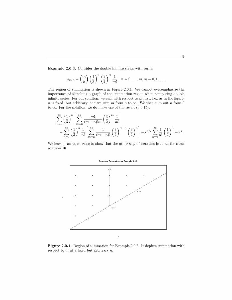
The region of summation is shown in Figure 2.0.1. We cannot overemphasize theimportance of sketching a graph of the summation region when computing doubleinfinite series. For our solution, we sum with respect to m first; i,e., as in the figure,n is fixed, but arbitrary, and we sum m from n to ∞. We then sum out n from 0to ∞. For the solution, we do make use of the result (3.0.15).

∞∑

n=0

(

1

3

)n[

∞∑

m=n

m!

(m− n)!n!

(

3

2

)m1

m!

]

=∞∑

n=0

(

1

3

)n1

n!

[

∞∑

m=n

1

(m− n)!

(

3

2

)m−n (3

2

)n]

= e3/2∞∑

n=0

1

n!

(

1

2

)n

= e2.

We leave it as an exercise to show that the other way of iteration leads to the samesolution.

n

m

( n, n )

m = n

Region of Summation for Example A.1.3

Figure 2.0.1: Region of summation for Example 2.0.3. It depicts summation withrespect to m at a fixed but arbitrary n.

Chapter 3

Derivatives

We assume that the reader is familiar with differentiable calculus. The followingdiscussion serves only as a brief review of it.

Let f(x) be a real valued function defined on an interval of real numbers (a, b)which can be (−∞,∞). Recall that f is differentiable at x with derivative f ′(x)if the following limit exists:

lim∆x→0

f(x+∆x)− f(x)

∆x= f ′(x). (3.0.1)

We often express f ′(x) as f ′(x) = ddxf(x). It follows immediately from this defini-

tion that if f(x) is differentiable at x then it is continuous at x.Next we list some useful formulas for derivatives. Their derivations can be found

in any calculus book. Assume that functions f(x) and g(x) are differentiable at x.

d

dxx = 1;

d

dxxr = rxr−1 (for r < 1 not differentiable at 0) (3.0.2)

d

dx[af(x) + bg(x)] = af ′(x) + bg′(x) (3.0.3)

d

dx[f(x)g(x)] = f ′(x)g(x) + f(x)g′(x) (3.0.4)

d

dx[f(x)/g(x)] = [f ′(x)g(x) − f(x)g′(x)]/g(x)2 (3.0.5)

d

dx[f(x)a)] = af ′(x)a−1 (3.0.6)

d

dxf [g(x)] = f ′[g(x)]g′(x) (3.0.7)

d

dxef(x) = f ′(x)ef(x) (3.0.8)

Assume in addition that f(x) is strictly increasing or decreasing on (a, b). Thenthe inverse function f−1(y) exists on (a, b) and its derivative is given by

d

dyf−1(y) =

1

f ′[f−1(y)]. (3.0.9)

11

12 Derivatives

Recall the Mean Value Theorem which is given by:

Theorem 3.0.1 (Mean Value Theorem). Let f(x) be continuous on the interval

[a, b] and differentiable on (a, b). Then there is a point ξ such that a < ξ < b and

f(b) = f(a) + (b− a)f ′(ξ). (3.0.10)

Note that if f(x) is differentiable in an open neighborhood of x0 and f ′(x) iscontinuous at x0 then for some ξ between x and x0 we can write equation (3.0.10)as

f(x) = f(x0) + (x− x0)f′(ξ)

= f(x0) + (x− x0)f′(x0) + (x − x0)[f

′(ξ)− f ′(x0)]

= f(x0) + (x− x0)f′(x0) + o(x − x0), (3.0.11)

where the little o notation is defined by

a = o(b) if and only if ab → 0 when b → 0. (3.0.12)

Suppose f ′(x) is differentiable; i.e., (d/dx)f ′(x) exists. Then we call this thesecond derivative of f(x) and write it as (d2/dx2)f(x) = f ′′(x) = f (2)(x). Con-tinuing in this way, if it exists, we denote the nth derivative of f(x) by f (n)(x) forn ≥ 1.

The mean value theorem provides a first-order approximation of f(x) in a neigh-borhood of x0. Higher order expansions are called Taylor series.

Theorem 3.0.2 (Taylor Series). Suppose that f(x) has at least n + 1 derivatives

in an open interval I of x0 and f (n+1) is continuous in I. Then for all x ∈ I there

is some ξ between x and x0 such that

f(x) = f(x0) +n∑

j=1

f (j)(x0)

j!(x− x0)

j +f (n+1)(ξ)

(n+ 1)!(x− x0)

n+1. (3.0.13)

For x0 = 0, a Taylor series is called a Maclaurin series.

The last term in the Taylor series, (3.0.13), is called the remainder of the series.Functions f(x) which are infinitely differentiable in an open interval I of x0 and forwhich the remainder goes to 0 as n → ∞ for all x ∈ I are said to be analytic in I.For these functions, f(x) is the infinite Taylor series; i.e., for all x ∈ I,

f(x) = f(x0) +

∞∑

n=1

f (n)(x0)

n!(x − x0)

n. (3.0.14)

13

Examples of analytic functions and their intervals of convergence are:

ex =

∞∑

n=0

xn

n!, −∞ < x < ∞, (3.0.15)

sin(x) =

∞∑

n=0

(−1)nx2n+1

(2n+ 1)!, −∞ < x < ∞, (3.0.16)

cos(x) =∞∑

n=0

(−1)nx2n

(2n)!, −∞ < x < ∞, (3.0.17)

(1− x)−r =

∞∑

n=0

(

n+ r − 1

r − 1

)

xn, , |x| < 1, r > 0. (3.0.18)

Partial Derivatives

For functions of several variables, we briefly discuss the concept of partial dif-

ferentiation. These derivatives are taken with respect to a variable while theother variables are held fixed. For the partial with respect to x, instead of thed/dx notation of the univariate case, we use the notation ∂/∂x. For example letf(x, y) = 2x2 exp{−x2 − y2}. Then

∂

∂xf(x, y) = 4x exp{−x2 − y2} − 4x3 exp{−x2 − y2}

∂

∂yf(x, y) = −4x2y exp{−x2 − y2}

Partial derivatives of the partials can be performed, also. These are called mixed

partials. Continuing with the last example, we have:

∂2

∂x∂yf(x, y) =

∂

∂y{ ∂

∂xf(x, y)} = −8xy exp{−x2 − y2}+ 8x3y exp{−x2 − y2}

∂2

∂y2f(x, y) = −4x2 exp{−x2 − y2}+ 8x2y2 exp{−x2 − y2}

For mixed partials, the order of differentiation does not matter as long as the partialsexist and are continuous. For instance, for such functions, (∂2/∂x∂y) f(x, y) =(∂2/∂y∂x) f(x, y).

Chapter 4

Integration

One way of motivating the process of integration of functions is to consider Rie-

mann sums. Let F (x) be a function defined on the interval [a, b]. Partition [a, b]into the n subintervals

[a+ (i− 1)∆x, a+ i∆x], i = 1, . . . , n; ∆x =b− a

n.

Let ξi be the midpoint of [a+(i−1)∆x, a+i∆x]. Then the correspondingRiemann

sum is

Rn = Rn(f, a, b,∆x) =

n∑

i=1

f(ξi)∆x. (4.0.1)

Note that this is an average. In calculus, it is proved that if f(x) is continuous on[a, b] then Rn converges to a limit as n → ∞ and we denote it as

limn→∞

Rn =

∫ b

a

f(x) dx. (4.0.2)

We call this limit1 the definite integral of f(x) over [a, b]. Also, if f(x) ≥ 0 on[a, b] then Rn is an approximation to the area under the curve y = f(x) between aand b. Hence, the area under the curve y = f(x) between a and b is defined as theintegral of f from a to b.

For many of the integrals in this text, the bounds in the interval [a, b] may beinfinite. For example, the integral of interest is

∫∞a f(x) dx. Provided the following

limit exists, the value of the integral is given by the limit

limh→∞

∫ h

a

f(x) dx =

∫ ∞

a

f(x) dx. (4.0.3)

In these cases, we have from the theory of calculus that

∫ b

a

|f(x)| dx < ∞ ⇒∫ b

a

f(x) dx exists, (4.0.4)

1The limit is the same for all subdivisions provided ∆x → 0.

15

16 Integration

that is, absolute convergence implies convergence.As the next theorem states integration is the process of anti-differentiation.

Theorem 4.0.1 (Fundamental Theorem of Calculus). Let the function F (x) be

differentiable on the interval [a, b] with derivative f(x). If f(x) is continuous on

[a, b] then

F (b)− F (a) =

∫ b

a

f(x) dx. (4.0.5)

For example, since xn is the derivative of xn+1/(n+ 1), we have

∫ b

a

xn dx =xn+1

n+ 1

∣

∣

∣

∣

b

a

=1

n+ 1[bn+1 − an+1].

The following is a list of properties of integration, (proofs of which can be foundin any calculus book). Assume that all the integrals exist.

∫ b

a

[cf(x) + dg(x)] dx = c

∫ b

a

f(x) dx + d

∫ b

a

g(x) dx (4.0.6)

a < c < b ⇒∫ b

a

f(x) dx =

∫ c

a

f(x) dx +

∫ b

c

f(x) dx (4.0.7)

∫ b

a

f(x) dx = −∫ a

b

f(x) dx (4.0.8)

f(x) ≥ g(x) on [a, b] ⇒∫ b

a

f(x) dx ≥∫ b

a

g(x) dx (4.0.9)

We often use the technique of change-of-variable to facilitate the computa-tion of an integral. Suppose that g(x) is differentiable on [a, b] and that F (x) isdifferentiable on the range of g(x). By the chain rule for differentiation, we have

Dx F [g(x)] = F ′[g(x)]g′(x).

So,

∫ b

a

F ′[g(x)]g′(x) dx = F [g(x)]

∣

∣

∣

∣

b

a

= F [g(b)]− F [g(a)] =

∫ g(b)

g(a)

F ′(u) du. (4.0.10)

This formulation is cumbersome, so we generally write the transformation as u =g(x) and use the notation du = g′(x) dx. For example, suppose we want to compute∫ 3

2x exp{−x2} dx. Let u = x2 then du = 2x dx and we obtain

∫ 3

2

x exp{−x2} dx =1

2

∫ 3

2

2x exp{−x2} dx =1

2

∫ 9

4

e−u du =1

2(e−4 − e−9).

For monotne transformations, the change-of-variable techniques produces a use-

ful formula. Consider∫ b

af(x) dx. Let y = g(x) denote a continuous and differen-

tiable transformation where g(x) is a strictly monotone function on [a, b]. Suppose

17

that g(x) is strictly decreasing. Then the transformation maps [a, b] into [g(b), g(a)].Note that x = g−1(y) and by (3.0.9),

dx

dy=

1

g′[g−1(y)].

Because g(x) is decreasing, dx/dy is negative and, hence, |dx/dy| = −dx/dy. So,by the change-of-variable technique and expression (4.0.8) we have

∫ b

a

f(x) dx =

∫ g(b)

g(a)

f [g−1(y)]dx

dydy =

∫ g(a)

g(b)

f [g−1(y)]

∣

∣

∣

∣

dx

dy

∣

∣

∣

∣

dy. (4.0.11)

This same formula holds if the transformation is strictly increasing.Another technique for computation of integrals is integration by parts. Let

u(x) and v(x) be differentiable functions on [a, b] whose second derivatives exist,also. By the product rule for differention (3.0.4),

d

dx[u(x)v(x)] = u′(x)v(x) + u(x)v′(x).

Integrating both sides and solving for the second term on the right, we have∫ b

a

u(x)v′(x) dx =

∫ b

a

d

dx[u(x)v(x)] dx −

∫ b

a

u′(x)v(x) dx

= u(x)v(x)

∣

∣

∣

∣

b

a

−∫ b

a

u′(x)v(x) dx. (4.0.12)

For instance, suppose we want to compute∫ b

a x exp{−x} dx. Take u(x) = x andv′(x) = exp{−x} then u′(x) = 1 and v(x) = − exp{−x} and we obtain

∫ b

a

xe−x dx = −xe−x |ba +∫ b

a

e−x dx = e−a(a+ 1)− e−b(b+ 1).

4.0.3 Multiple Integration

The concept of integration can be extended to n-dimensions. We shall briefly reviewits generalizationto two dimensions. Let f(x, y) be a continuous function of twovariables which is defined on a bounded rectangle A. In this setting, the conceptof a Reimann sum easily generaizes and we only briefly discuss it. Partition A intomn subrectangles and form the sum over all the subrectangles (i, j),

Rm,n = Rm,n(f,A,∆x,∆y) =

m∑

i=1

n∑

j=1

f(xi, yj)∆xi∆yj , (4.0.13)

where (xi, yj) is a point in the interior of the (i, j)th rectangle. If the largest diagonalof the subrectangles converges to 0 as m and n converge to ∞, then Rm,n has alimit which we call the double integral of f over A and write it as

∫∫

A

f(x, y) dxdy.

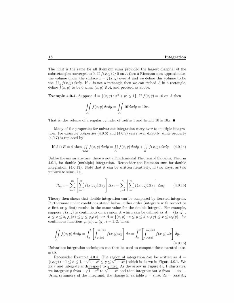
18 Integration

The limit is the same for all Riemann sums provided the largest diagonal of thesubrectangles converges to 0. If f(x, y) ≥ 0 on A then a Riemann sum approximatesthe volume under the surface z = f(x, y) over A and we define this volume to bethe

∫∫

A f(x, y) dxdy. If A is not a rectangle then we can embed A in a rectangle,define f(x, y) to be 0 when (x, y) 6∈ A, and proceed as above.

Example 4.0.4. Suppose A = {(x, y) : x2 + y2 ≤ 1}. If f(x, y) = 10 on A then

∫∫

A

f(x, y) dxdy =

∫∫

A

10 dxdy = 10π.

That is, the volume of a regular cylinder of radius 1 and height 10 is 10π.

Many of the properties for univariate integration carry over to multiple integra-tion. For example properties (4.0.6) and (4.0.9) carry over directly, while property(4.0.7) is replaced by

If A ∩B = φ then∫∫

A∪B

f(x, y) dxdy =∫∫

A

f(x, y) dxdy +∫∫

B

f(x, y) dxdy. (4.0.14)

Unlike the univariate case, there is not a Fundamental Theorem of Calculus, Theorm4.0.1, for double (multiple) integration. Reconsider the Reimann sum for doubleintegration, (4.0.13). Note that it can be written iteratively, in two ways, as twounivariate sums, i.e.,

Rm,n =

m∑

i=1

n∑

j=1

f(xi, yj)∆yj

∆xi =

n∑

j=1

[

m∑

i=1

f(xi, yj)∆xi

]

∆yj. (4.0.15)

Theory then shows that double integration can be computed by iterated integrals.Furthermore under conditions stated below, either order (integrate with respect tox first or y first) results in the same value for the double integral. For example,suppose f(x, y) is continuous on a region A which can be defined as A = {(x, y) :a ≤ x ≤ b, ϕ1(x) ≤ y ≤ ϕ2(x)} or A = {(x, y) : c ≤ y ≤ d, ω1(y) ≤ x ≤ ω2(y)} forcontinuous functions ϕi(x), ωi(y), i = 1, 2. Then

∫∫

A

f(x, y) dxdy =

∫ b

a

[

∫ ϕ2(x)

ϕ1(x)

f(x, y) dy

]

dx =

∫ d

c

[

∫ ω2(y)

ω1(y)

f(x, y) dx

]

dy.

(4.0.16)Univariate integration techniques can then be used to compute these iterated inte-grals.

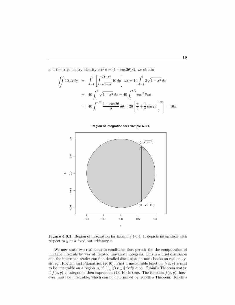
Reconsider Example 4.0.4. The region of integration can be written as A ={(x, y) : −1 ≤ x ≤ 1,−

√1− x2 ≤ y ≤

√1− x2} which is shown in Figure 4.0.1. We

fix x and integrate with respect to y first. As the arrow in Figure 4.0.1 illustrates,we integrate y from −

√1− x2 to

√1− x2 and then integrate out x from −1 to 1..

Using symmetry of the integrand; the change-in-variable x = sin θ, dx = cos θ dx;

19

and the trigonmetry identity cos2 θ = (1 + cos 2θ)/2, we obtain

∫∫

A

10 dxdy =

∫ 1

−1

[

∫

√1−x2

−√1−x2

10 dy

]

dx = 10

∫ 1

−1

2√

1− x2 dx

= 40

∫ 1

0

√

1− x2 dx = 40

∫ π/2

0

cos2 θ dθ

= 40

∫ π/2

0

1 + cos 2θ

2dθ = 20

[

π

2+

1

2sin 2θ

∣

∣

∣

∣

π/2

0

]

= 10π.

−1.0 −0.5 0.0 0.5 1.0

−1.

0−

0.5

0.0

0.5

1.0

x

y

( x, − 1 − x2 )

( x, 1 − x2 )

Region of Integration for Example A.3.1.

Figure 4.0.1: Region of integration for Example 4.0.4. It depicts integration withrespect to y at a fixed but arbitrary x.

We now state two real analysis conditions that permit the the computation ofmultiple integrals by way of iterated univariate integrals. This is a brief discussionand the interested reader can find detailed discussions in most books on real analy-sis; eg., Royden and Fitzpatrick (2010). First a measurable function f(x, y) is saidto be integrable on a region A, if

∫∫

A|f(x, y)| dxdy < ∞. Fubini’s Theorem states:

if f(x, y) is integrable then expression (4.0.16) is true. The function f(x, y), how-ever, must be integrable, which can be determined by Tonelli’s Theorem. Tonelli’s

20 Integration

Theorem states that if f(x, y) is a non-negative measurable function on A then thedouble integral of f(x, y) can be computed iteratively. Hence, Tonelli’s Theoremis used to establish that the integral of |f(x, y)| is finite, then Fubini’s Theorem isused to compute the double integral of f(x, y) via iterated integrals. Note that allfunctions used in this text are measurable; see Royden and Fitzpatrick (2010) fordiscussions on measurable functions.

Expression (4.0.16) gives us a choice on which variable is integrated first. ForExample 4.0.4, because of the symmetry of x and y in the problem, it does notmatter. In certain cases, however, a little thought before selecting the order canlead to an easier solution. Our next example is one such case. It helps considerablyin performing double integrations to always sketch the region of integration first.

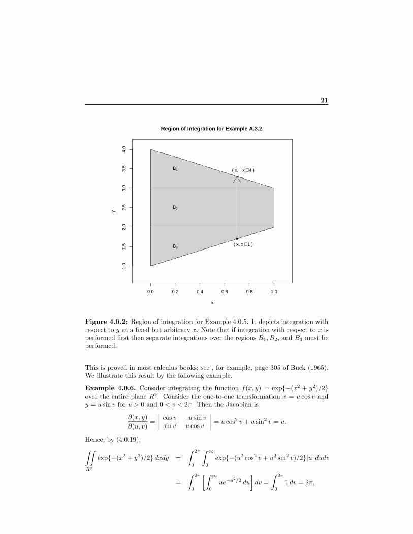
Example 4.0.5. The region A = {(x, y) : 0 < x < 1, x + 1 < y < −x + 4} issketched in Figure 4.0.2. Suppose we want to compute

∫∫

Ax2y dxdy. From the

figure, if we integrate with respect to y then for any fixed x, 0 < x < 1, we needto integrate from y = x + 1 to y = −x + 4 and then integrate out x from 0 to 1.On the other hand, suppose we decide to intergate with respect to x first. Then,as shown in the figure, the integration over the three regions B1, B2, and B3 mustbe computed. Since the regions are disjoint,

∫∫

Ax2y dxdy is the sum of these three

integrals. We choose to integrate with respect to y first.

∫∫

A

x2y dxdy =

∫ 1

0

x2

[∫ −x+4

x+1

y dy

]

dx =1

2

∫ 1

0

x2[

(−x+ 4)2 − (x+ 1)2]

dx

=1

2

∫ 1

0

(−10x3 + 15x2) dx =5

4.

If we intergate with respect to x first then by the figure the double integration is:

∫∫

A

x2ydxdy =

∫ 2

1

y

[∫ y−1

0

x2dx

]

dy+

∫ 3

2

y

[∫ 1

0

x2 dx

]

dy+

∫ 4

3

y

[∫ 4−y

0

x2dx

]

dy.

(4.0.17)The reader is asked to show that ?????????EXER??? these integrations result inthe above answer 5/4.

There is a multiple variable analog to the change-in-variable technique for uni-variate integration for a one-to-one transformation; see discussion around expres-sions (4.0.10) and (4.0.11). Suppose we are intergrating the function f(x, y) overthe region D. Let (u, v) = T (x, y) be a one-to-one transformation from D to T (D).Define the Jacobian of the transformation to be the determinant

∂(x, y)

∂(u, v)=

∣

∣

∣

∣

∂x∂u

∂x∂v

∂y∂u

∂y∂v

∣

∣

∣

∣

=∂x

∂u

∂y

∂v− ∂x

∂v

∂y

∂u. (4.0.18)

Then the multivariate analog of expression (4.0.11) is∫∫

D

f(x, y) dxdy =

∫∫

T (D)

f[

T−1(u, v)]

∣

∣

∣

∣

∂(x, y)

∂(u, v)

∣

∣

∣

∣

dudv. (4.0.19)

21

0.0 0.2 0.4 0.6 0.8 1.0

1.0

1.5

2.0

2.5

3.0

3.5

4.0

x

y

( x, x + 1 )

( x, − x + 4 )B1

B2

B3

Region of Integration for Example A.3.2.

Figure 4.0.2: Region of integration for Example 4.0.5. It depicts integration withrespect to y at a fixed but arbitrary x. Note that if integration with respect to x isperformed first then separate integrations over the regions B1, B2, and B3 must beperformed.

This is proved in most calculus books; see , for example, page 305 of Buck (1965).We illustrate this result by the following example.

Example 4.0.6. Consider integrating the function f(x, y) = exp{−(x2 + y2)/2}over the entire plane R2. Consider the one-to-one transformation x = u cos v andy = u sin v for u > 0 and 0 < v < 2π. Then the Jacobian is

∂(x, y)

∂(u, v)=

∣

∣

∣

∣

cos v −u sin vsin v u cos v

∣

∣

∣

∣

= u cos2 v + u sin2 v = u.

Hence, by (4.0.19),

∫∫

R2

exp{−(x2 + y2)/2} dxdy =

∫ 2π

0

∫ ∞

0

exp{−(u2 cos2 v + u2 sin2 v)/2}|u| dudv

=

∫ 2π

0

[∫ ∞

0

ue−u2/2 du

]

dv =

∫ 2π

0

1 dv = 2π,

22 Integration

where before the last equality the univariate transformation z = u2/2 can be usedto show that the inner integral is 1.