MathematicalMethodsforWirelessChannelEstimationand ... · PDF fileMathematicalMethodsforWirelessChannelEstimationand Equalization Verfasser ... (IEEE 802.11p) erfordern die ... well

DISSERTATION

Titel der Dissertation

Mathematical Methods for Wireless Channel Estimation and

Equalization

Verfasser

Saptarshi Das

angestrebter akademischer Grad

Doktor der Naturwissenschaften

Wien, August 2009

Studienkennzahl lt. Studienblatt: A 091 405

Studienrichtung lt. Studienblatt: Mathematik

Betreuer: Prof. Dr. Hans G. Feichtinger

ii

Contents

Preface vii

Acknowledgements ix

1 Introduction 1

1.1 Overview . . . . . . . . . . . . . . . . . . . . . . . . . . . . . . . . . . . . . . . . . . . . . 1

1.2 Motivation . . . . . . . . . . . . . . . . . . . . . . . . . . . . . . . . . . . . . . . . . . . . 1

1.3 Previous Work . . . . . . . . . . . . . . . . . . . . . . . . . . . . . . . . . . . . . . . . . . 2

1.3.1 Channel Estimation . . . . . . . . . . . . . . . . . . . . . . . . . . . . . . . . . . . 2

1.3.2 Equalization . . . . . . . . . . . . . . . . . . . . . . . . . . . . . . . . . . . . . . . 3

1.4 Contributions . . . . . . . . . . . . . . . . . . . . . . . . . . . . . . . . . . . . . . . . . . . 4

2 Mathematical Models 7

2.1 Introduction . . . . . . . . . . . . . . . . . . . . . . . . . . . . . . . . . . . . . . . . . . . . 7

2.2 Transmission Setup: Frequency Modulation . . . . . . . . . . . . . . . . . . . . . . . . . . 7

2.3 OFDM Model . . . . . . . . . . . . . . . . . . . . . . . . . . . . . . . . . . . . . . . . . . . 9

2.4 Mathematical Models of Wireless Channel . . . . . . . . . . . . . . . . . . . . . . . . . . . 11

2.5 Channel Matrix . . . . . . . . . . . . . . . . . . . . . . . . . . . . . . . . . . . . . . . . . . 15

2.6 Formulation of the Problems . . . . . . . . . . . . . . . . . . . . . . . . . . . . . . . . . . 18

2.6.1 Channel Estimation . . . . . . . . . . . . . . . . . . . . . . . . . . . . . . . . . . . 18

2.6.2 Equalization . . . . . . . . . . . . . . . . . . . . . . . . . . . . . . . . . . . . . . . 19

2.7 Related Mathematical Research Areas . . . . . . . . . . . . . . . . . . . . . . . . . . . . . 20

2.7.1 Resolution of the Gibbs Phenomenon . . . . . . . . . . . . . . . . . . . . . . . . . 20

2.7.2 Solution of Linear Systems . . . . . . . . . . . . . . . . . . . . . . . . . . . . . . . 21

2.7.3 Krylov Subspace Based Methods . . . . . . . . . . . . . . . . . . . . . . . . . . . . 21

2.7.4 Preconditioning . . . . . . . . . . . . . . . . . . . . . . . . . . . . . . . . . . . . . . 23

2.7.5 Effective Numerical Precision . . . . . . . . . . . . . . . . . . . . . . . . . . . . . . 24

2.7.6 Other Related Research . . . . . . . . . . . . . . . . . . . . . . . . . . . . . . . . . 25

2.8 Measurements of Transmission Quality . . . . . . . . . . . . . . . . . . . . . . . . . . . . . 26

iii

3 Channel Estimation and Equalization: Classical and Contemporary Algorithms 27

3.1 Introduction . . . . . . . . . . . . . . . . . . . . . . . . . . . . . . . . . . . . . . . . . . . . 27

3.2 Channel Estimation . . . . . . . . . . . . . . . . . . . . . . . . . . . . . . . . . . . . . . . 27

3.3 Frequency Selective Channel . . . . . . . . . . . . . . . . . . . . . . . . . . . . . . . . . . . 28

3.4 Pilot Arrangement . . . . . . . . . . . . . . . . . . . . . . . . . . . . . . . . . . . . . . . . 28

3.5 Frequency Domain Channel Estimation . . . . . . . . . . . . . . . . . . . . . . . . . . . . 31

3.6 Time Domain Channel Estimation . . . . . . . . . . . . . . . . . . . . . . . . . . . . . . . 32

3.7 Doubly-Selective Channels . . . . . . . . . . . . . . . . . . . . . . . . . . . . . . . . . . . . 34

3.8 Basis Expansion Model . . . . . . . . . . . . . . . . . . . . . . . . . . . . . . . . . . . . . 34

3.9 Equalization . . . . . . . . . . . . . . . . . . . . . . . . . . . . . . . . . . . . . . . . . . . . 36

3.9.1 Single-tap Equalization . . . . . . . . . . . . . . . . . . . . . . . . . . . . . . . . . 36

3.9.2 Doubly Selective Channel Equalization . . . . . . . . . . . . . . . . . . . . . . . . . 37

3.10 Simulation Setup . . . . . . . . . . . . . . . . . . . . . . . . . . . . . . . . . . . . . . . . . 38

3.11 Results of Simulations . . . . . . . . . . . . . . . . . . . . . . . . . . . . . . . . . . . . . . 38

4 Estimation of rapidly varying channels in OFDM systems using a BEM with Legendre

polynomials 41

4.1 Introduction . . . . . . . . . . . . . . . . . . . . . . . . . . . . . . . . . . . . . . . . . . . . 41

4.1.1 Overview . . . . . . . . . . . . . . . . . . . . . . . . . . . . . . . . . . . . . . . . . 41

4.1.2 Motivation and Previous Work . . . . . . . . . . . . . . . . . . . . . . . . . . . . . 42

4.1.3 Contributions . . . . . . . . . . . . . . . . . . . . . . . . . . . . . . . . . . . . . . . 42

4.2 Theoretical Foundations of the Estimation Algorithm . . . . . . . . . . . . . . . . . . . . 43

4.2.1 Overview . . . . . . . . . . . . . . . . . . . . . . . . . . . . . . . . . . . . . . . . . 43

4.2.2 Fourier Coefficients of Channel Taps . . . . . . . . . . . . . . . . . . . . . . . . . . 43

4.2.3 BEM with Legendre Polynomials . . . . . . . . . . . . . . . . . . . . . . . . . . . . 44

4.3 System Model . . . . . . . . . . . . . . . . . . . . . . . . . . . . . . . . . . . . . . . . . . . 46

4.3.1 Transmitter-Receiver Model . . . . . . . . . . . . . . . . . . . . . . . . . . . . . . . 46

4.3.2 BEM with Legendre Polynomials . . . . . . . . . . . . . . . . . . . . . . . . . . . . 47

4.4 Proposed Channel Estimator . . . . . . . . . . . . . . . . . . . . . . . . . . . . . . . . . . 47

4.4.1 Analysis of Intercarrier Interactions . . . . . . . . . . . . . . . . . . . . . . . . . . 47

4.4.2 Pilot Arrangement . . . . . . . . . . . . . . . . . . . . . . . . . . . . . . . . . . . . 48

4.4.3 Estimation of Fourier Coefficients . . . . . . . . . . . . . . . . . . . . . . . . . . . . 48

4.4.4 Estimation of Legendre Coefficients . . . . . . . . . . . . . . . . . . . . . . . . . . 50

4.4.5 Algorithm Summary and Complexity . . . . . . . . . . . . . . . . . . . . . . . . . . 51

4.5 Numerical Simulations . . . . . . . . . . . . . . . . . . . . . . . . . . . . . . . . . . . . . . 52

4.5.1 Simulation Setup . . . . . . . . . . . . . . . . . . . . . . . . . . . . . . . . . . . . . 52

4.5.2 Results of Simulations . . . . . . . . . . . . . . . . . . . . . . . . . . . . . . . . . . 53

4.6 Chapter Conclusions . . . . . . . . . . . . . . . . . . . . . . . . . . . . . . . . . . . . . . . 53

iv

5 Low Complexity Equalization for Doubly Selective Channels Modeled by a Basis

Expansion 57

5.1 Introduction . . . . . . . . . . . . . . . . . . . . . . . . . . . . . . . . . . . . . . . . . . . . 57

5.1.1 Overview . . . . . . . . . . . . . . . . . . . . . . . . . . . . . . . . . . . . . . . . . 57

5.1.2 Motivation and Previous Work . . . . . . . . . . . . . . . . . . . . . . . . . . . . . 58

5.1.3 Contributions . . . . . . . . . . . . . . . . . . . . . . . . . . . . . . . . . . . . . . . 59

5.2 System Model . . . . . . . . . . . . . . . . . . . . . . . . . . . . . . . . . . . . . . . . . . . 59

5.2.1 Transmission Model . . . . . . . . . . . . . . . . . . . . . . . . . . . . . . . . . . . 59

5.2.2 Wireless Channel Representation with BEM . . . . . . . . . . . . . . . . . . . . . . 60

5.2.3 Equivalence of the BEM and the Product-Convolution Representation . . . . . . . 61

5.3 Equalization . . . . . . . . . . . . . . . . . . . . . . . . . . . . . . . . . . . . . . . . . . . . 61

5.3.1 Iterative Equalization Methods . . . . . . . . . . . . . . . . . . . . . . . . . . . . . 61

5.3.2 Preconditioning . . . . . . . . . . . . . . . . . . . . . . . . . . . . . . . . . . . . . . 62

5.4 Description of the Algorithm . . . . . . . . . . . . . . . . . . . . . . . . . . . . . . . . . . 63

5.4.1 Decomposition of Channel Matrix . . . . . . . . . . . . . . . . . . . . . . . . . . . 63

5.4.2 Algorithm . . . . . . . . . . . . . . . . . . . . . . . . . . . . . . . . . . . . . . . . . 65

5.4.3 Computational Complexity . . . . . . . . . . . . . . . . . . . . . . . . . . . . . . . 65

5.4.4 Memory . . . . . . . . . . . . . . . . . . . . . . . . . . . . . . . . . . . . . . . . . . 66

5.5 Numerical Simulations . . . . . . . . . . . . . . . . . . . . . . . . . . . . . . . . . . . . . . 67

5.5.1 Simulation Setup . . . . . . . . . . . . . . . . . . . . . . . . . . . . . . . . . . . . . 67

5.5.2 Discussion of Results . . . . . . . . . . . . . . . . . . . . . . . . . . . . . . . . . . . 67

5.6 Chapter Conclusions . . . . . . . . . . . . . . . . . . . . . . . . . . . . . . . . . . . . . . . 70

Conclusions 75

v

vi

Preface

English

Reliable and fast transmission of information over rapidly varying wireless channels is necessary for mod-

ern and upcoming wireless applications, like mobile-WiMAX (IEEE 802.16e), WAVE (IEEE 802.11p).

The variability of wireless channels is mainly due to the multipath effect and the Doppler effect. The

Doppler effect is typically caused by mobility between the receiver and the transmitter. For integrity of

such communications, accurate wireless channel estimation and equalization are crucial. In this disserta-

tion, we address the problems of wireless channel estimation and equalization for transmission through

rapidly varying wireless channels using the OFDM system.

A wireless channel is modeled as a pseudo-differential operator. The problem of channel estimation

is to approximately identify the operator in question. Furthermore, the problem of equalization is to

approximately identify the transmitted signal from the received signal and the estimated wireless channel.

However, for practical computations with discrete digital signals, the pseudo-differential operator is

approximated with a matrix, known as the wireless channel matrix. The wireless channel matrix in the

time domain represents time-varying convolution with a time-varying filter. Basis Expansion Models

(BEM) are used to model rapidly varying wireless channels, with each time-varying convolution filter

coefficient modeled as a linear combination of certain basis functions. Within the framework of the BEM,

channel estimation amounts to computing the basis coefficients for the representation of the time varying

filter.

In this dissertation, we propose novel methods for wireless channel estimation in the framework of the

BEM. Furthermore, we propose a novel method for equalization using the estimated BEM coefficients.

The proposed equalization methods do not create the channel matrix, but use the estimated BEM

coefficients directly. Furthermore, we propose a suitable preconditioner for the proposed equalization.

With K OFDM subcarriers, and L discrete path delays, i.e. L discrete time varying filter coefficients,

the proposed wireless channel estimation and equalization method requires, O(L logL) and O(K logK)

in operations, and O(L) and O(K) in memory respectively. Computer simulation shows the superior-

ity of the proposed methods with respect to the conventional and contemporary methods in terms of

performance and complexity. The computer simulations comply with the IEEE 802.16e standard.

vii

German

Derzeit in Verwendung befindliche und zukunftige drahtlose Kommunikationssysteme wie Mobile-WiMAX

(IEEE 802.16e) oder WAVE (IEEE 802.11p) erfordern die zuverlassige und schnelle Ubermittlung von In-

formation uber rasch veranderliche drahtlose Ubertragungskanale. Die Variabilitat von Drahtloskanalen

beruht hauptsachlich auf Mehrwegempfang und Dopplereffekt, wobei letzterer typischerweise durch Mo-

bilitat des Empfangers bzw. des Senders verursacht wird. Um die Integritat solcher Ubertragungen

sicherstellen zu konnen, sind moglichst genau Kanalschatzung und -entzerrung ganz wesentlich.

In der vorliegenden Dissertation werden die Probleme der Kanalschatzung und Kanalentzerrung fur

Ubertragungen uber rasch veranderliche Drahtloskanale (auf der Basis von OFDM-Systemen) behandelt.

Ein drahtloser Ubertragungskanal wird als Pseudodifferentialoperator modelliert. Das Problem der

Kanalschatzung besteht in der naherungsweisen Identifikation dieses Operators. Unter Entzerrung ver-

steht man die naherungsweise Bestimmung des gesendeten Signals aus dem empfangenen Signal und

dem geschatzten Drahtloskanal. In der Praxis wird der Pseudodifferentialoperator fur Berechnungen

mit diskreten Zeitsignalen naherungsweise durch eine Matrix ersetzt, die so genannte Drahtloskanal-

matrix. Im Zeitbereich reprasentiert die Drahtloskanalmatrix eine zeitabhangige Faltung mit einem

zeitabhangigen Filter. Zur Modellierung schnell veranderlicher Drahtloskanale verwendet man Basisen-

twicklungsmodelle (BEM), wobei jeder zeitabhangige Faltungsfilterkoeffizient als Linearkombination bes-

timmter Basisfunktionen modelliert wird. Im Rahmen der BEM lauft Kanalschatzung auf die Berechnung

der Entwicklungskoeffizienten fur die Darstellung der zeitabhangigen Filter hinaus.

In dieser Dissertation werden neue Methoden der Kanalschatzung im Rahmen von BEM vorgeschla-

gen. Die hiermit gewonnenen BEM-Koeffizienten werden daruberhinaus direkt fur eine neue Methode

der Entzerrung eingesetzt, welche ohne die Erzeugung der Kanalmatrix auskommt.

Es wird auch auf die numerische Effizienz des vorgeschlagenen Schatzers Wert gelegt, beispielsweise

durch die Beistellung eines passenden Prakonditionierers fur die vorgeschlagenen Entzerrungsmethode.

Mit K OFDM-Teiltragern und L diskreten Pfadverzogerungen, d.h. L diskreten zeitabhangigen Filterko-

effizienten, benotigt die vorgeschlagene Methode zur Kanalschatzung und Entzerrung O(L logL) und

O(K logK) Operationen bzw. O(L) und O(K) Speicher. Computersimulationen gemaß IEEE 802.16e-

Standard bestatigen die Uberlegenheit der vorgeschlagenen Methode uber herkommliche und zur Zeit in

Verwendung befindliche Methoden in Bezug auf Leistung und Komplexitat.

viii

Acknowledgements

This work was possible due to the guidance and support of many people. First, I would like to acknowl-

edge my advisor Prof. Hans G. Feichtinger. He has taught me many things related to time-frequency

analysis and signal processing. I have greatly appreciated his hospitality at the Numerical Harmonic

Analysis Group (NuHAG) of University of Vienna. I would also like to especially acknowledge Dr.

Tomasz Hrycak. He has taught me a great deal about numerical mathematics (especially through his

well written MATLAB codes). He introduced to me many directions and questions related to numerical

analysis and signal processing, some which are addressed in this dissertation. He has never accepted any

assertion that I have made without some sort of proof, forcing me to think deeply. I am grateful to have

such a colleague. Also, I would like to thank Prof. Gerald Matz for his valuable suggestions, and time.

I must acknowledge all of the professors whom I have taken classes from, both at the University

of Vienna and Indian Institute of Technology, Bombay. At University of Vienna Prof. Arnold Neu-

maier taught me a great deal about numerical methods for practical data analysis, and Prof. Karlheinz

Groechenig gave me various useful suggestions regarding my progress at IK seminars. At Indian Institute

of Technology, Bombay, Prof. Amit Mitra introduced me to the field of signal processing for the first

time, Prof. Sachin Patkar taught me how to develop precise algorithms and data structures.

Working, playing, living, and arguing with my fellow colleagues at NuHAG has been both enriching

and enjoyable. I would like to thank my NuHAG colleagues: Julio, Harald, Gino, Anna, Nina, Alex,

Roza, Gerard, Sigrid, Ivana, Jose, Andreas, Darian, Elmar, Sebastian, Daniel, Jasminko. Discussion with

them at the lunch table, and after lunch coffee time were insightful, and fun. Especially, I would again

like to thank Prof. Feichtinger for building up such a working group and environment for conducting

research.

I would like to thank some of my fellow mates at Indian Institute of Technology, Bombay, especially:

Amar, Sumit, Sunil, Mousumi, Abdulla, Rajesh, Guruprashad, Mohit, Manish, Arindam, Chiranjeev,

Chiranjeet, Arif, and Anshuk. Before starting graduate school, I was fortunate to be an Associate at

Morgan Stanley. I would like to thank my former colleagues Saion, Anshuman, Dev, Thomson, Gunjan,

Maneesh and many more. From them, I learned a great deal about how to be professional.

Support of my family was crucial for me to come up with this dissertation. My parents Ruma and

Swapan Kr. Das, have been as supportive and loving as I could ever hope for, and I have learned a

great deal from their worldly wisdom. Most of all, I would like to acknowledge my wife Moumita, for her

ix

support, and understanding. I would also like to thank my sister, Sudeshna, and my extended family:

Morison Sourav, Dadabhai Anirvan, Didibhai Anindita, Anindya, Partha, Kakamoni, Sonakaku, Bulbuli,

Mani, Sonama, Monima, Mammam, Sejo Bhai, for their love and support.

Finally, I would like to acknowledge the Initiativkolleg, graduate school program of the University of

Vienna, for granting me the scholarship. I must acknowledge the Modern Harmonic Analysis Methods

for Advanced Wireless Communications (MOHAWI) project for partially funding my research.

Saptarshi Das

Vienna

August 01, 2009

x

Chapter 1

Introduction

1.1 Overview

In a general setup of a wireless communication system, the transmit signal passes through the wireless

medium and reaches the receiver. The wireless medium is generally called the wireless channel. Wire-

less channels are mathematically modeled as pseudo-differential operators. In this framework, wireless

channel estimation amounts to approximately identifying the operator, and equalization amounts to ap-

proximately computing the operand, i.e. the transmit signal, using the estimated kernel and the output

of the operation, i.e. the receive signal. With the current technology, reception of the mobile WiMAX

(IEEE 802.16e) in the proximity of a highway is unreliable because of the Doppler effect due to user

mobility, which dramatically hinder the quality of service (QoS). The QoS depends mainly on wire-

less channel estimation, equalization and signal encoding. In this dissertation, we address problems of

channel estimation and equalization for the Orthogonal Frequency Division Multiplexing (OFDM) based

communication systems over rapidly varying wireless channels, like mobile WiMAX. We use established

mathematical models describing the wireless channels and communication systems. As a contribution to

the wireless communication technology, we propose novel algorithms for channel estimation and equal-

ization for systems using the OFDM setup with severe channel distortions.

1.2 Motivation

In an ideal setup, the receive signal is a scaled version of the transmit signal. In practical setup, the

transmit signal is distorted by multipath propagation, Doppler’s effect due to relative motion between

the receiver and the transmitter, carrier frequency offset, and random noise. As a mathematical model,

the channel is commonly represented as a pseudo-differential operator acting on the transmit signal.

For computational purposes a discrete version of the operator is used, which is known as the channel

matrix. The dimensions of the channel matrix are determined by the sampling rate of the signal. Due

to increasing mobility between the receiver and the transmitter, the multipath delay and the Doppler

1

effect are severe, which makes the wireless channel estimation and equalization more challenging.

Orthogonal frequency-division multiplexing (OFDM), essentially identical to Coded OFDM (COFDM)

and Discrete multi-tone modulation (DMT), is a frequency-division multiplexing (FDM) scheme utilized

as a digital multi-carrier modulation method. A large number of closely-spaced orthogonal sub-carriers

are used to carry data. The data is divided into several parallel data streams or channels, one for each

sub-carrier. Each sub-carrier is modulated with a conventional modulation scheme (such as quadrature

amplitude modulation or phase shift keying) at a low symbol rate, maintaining total data rates similar

to conventional single-carrier modulation schemes in the same bandwidth. OFDM is increasingly used

in high-mobility wireless communication systems, e.g. mobile WiMAX (IEEE 802.16e), WAVE (IEEE

802.11p), and 3GPP’s UMTS Long-Term Evolution (LTE). Usually OFDM systems are designed so that

no Doppler effect occurs within an individual OFDM symbol duration. In this case, the channel acts

like a convolution with a finite filter. That is, the pseudo-differential operator modeling the wireless

channel reduces to a Fourier multiplier. Channel estimation and equalization is much simpler in such

a case. Recently, however, there has been an increasing interest in channels changing noticeably within

a single OFDM symbol. Typical reasons for such variations are increased user mobility and substantial

carrier frequency offsets, resulting in significant Doppler shifts and intercarrier interference (ICI). In-

tercarrier interference is especially detrimental to applications like DVB-T and mobile WiMAX, which

were originally designed for fixed receivers. For such a wireless channel, the kernel of the pseudo differ-

ential operator is more complicated, which makes channel estimation and equalization quite challenging.

Moreover, typical OFDM applications have very short OFDM symbol durations (e.g. 102.9 µs for mobile

WiMAX according to the standard IEEE 802.16e), and require fast algorithms for channel estimation

and equalization.

1.3 Previous Work

1.3.1 Channel Estimation

Channel estimation is the problem of approximately reconstructing the wireless channel. For practical

purposes, approximate values of the channel matrix, or parameters which determine the channel matrix

are computed. For channel estimation with an OFDM setup, only selected frequencies (pilot carriers)

are modulated with known values (pilot values) at the transmitter. At the receiver, information about

the pilot carriers and pilot values is used to estimate the channel. This type of estimation is known

as pilot-aided estimation. Channel estimation methods, which do not use pilot information for channel

estimation are called blind estimation methods. We do not consider blind estimation in this work.

Wireless channels, which arise only due to multipath propagation of electromagnetic waves and do

not vary over a certain duration of time, are modeled with a convolution operator. That is, the pseudo-

differential operator modeling the wireless channel reduces to a Fourier multiplier. Such channels are

examples of finite impulse response (FIR) filters. In the frequency domain, such channel operators are

2

diagonal, so they are also known as frequency selective channels. Pilot-aided estimation of frequency

selective channels is well known, see [23, 10], and is used in many applications, like WiFi (IEEE 802.11).

With increasing user mobility, the wireless channels are no more frequency selective, and such wireless

channels are called doubly selective.

For doubly selective channels, basis expansion models (BEM) are becoming popular. Within the

framework of the BEM, the discrete channel taps are modeled as time-varying functions, thus the BEM

models a doubly selective channel as a time varying filter. With the BEM, the channel taps are ap-

proximated by linear combinations of prescribed basis functions, see [49, 15, 54, 45, 46, 42]. In this

context, channel estimation amounts to approximate computation of the basis coefficients. The BEM

with complex exponential (CE-BEM) [49, 15, 9, 20] uses a truncated Fourier series, and is remarkable

because the resulting frequency-domain channel matrix is banded. However, this method has a limited

accuracy due to a large modeling error. Specifically, [53, 54] observe that the reconstruction with a trun-

cated Fourier series introduces significant distortions at the ends of the data block. The errors are due

to the Gibbs phenomenon, and manifest themselves as a spectral leakage, especially in the presence of

significant Doppler spreads. A more suitable exponential basis is provided by the Generalized CE-BEM

(GCE-BEM) [29], which employs complex exponentials oversampled in the frequency domain. A basis

of discrete prolate spheroidal wave functions is discussed in [53, 54]. Finally, the polynomial BEM (P-

BEM) is presented in [6]. For channels varying at the scale of one OFDM symbol duration, pilot-aided

channel estimation is studied in [45]. Definitive references on pilot-aided transmission in doubly-selective

channels are [26, 27].

1.3.2 Equalization

Frequency selective channel operators are diagonal in the frequency domain. In this case, the signal is

equalized by pointwise division of the receive signal by the frequency-domain channel attenuation values.

In the presence of additive uncorrelated noise, such equalization of the signal is optimal in the least

square (LS) sense. This type of equalization is known as single tap equalization.

For a doubly selective channel with severe ICI, conventional single-tap equalization in the frequency

domain is unreliable, see [36, 30, 38]. Several other approaches have been proposed to combat ICI

in transmissions over rapidly varying channels. For example, [8] presents minimum mean-square error

(MMSE) and successive interference cancellation equalizers, which use all subcarriers simultaneously.

Alternatively, using only a few subcarriers for equalization amounts to approximating the frequency-

domain channel matrix by a banded matrix, and has been exploited for equalizer design, see [47, 37].

ICI-shaping, which concentrates the ICI power within a small band of the channel matrix, is described

in [47, 41]. A low-complexity time-domain equalizer based on the LSQR algorithm is introduced in [22].

3

Figure 1.1: Position of wireless technologies in terms of data speed and mobility

1.4 Contributions

In this dissertation, we propose novel algorithms for wireless channel estimation and equalization for

OFDM based systems. Our algorithms are aimed to achieve a high data transfer rate despite high

user mobility. Fig. 1.1 shows the position of common wireless applications in terms of speed of data

delivery and mobility. Proposed estimation and equalization algorithms are suitable for all OFDM based

applications, like mobile-WiMAX which conforms to IEEE 802.16e standard, WAVE which conforms to

the IEEE 802.11p standard.

As a contribution to channel estimation, we propose a very efficient method for computation of the

Fourier coefficients of the channel taps using pilot information. A direct reconstruction of the channel

taps as truncated Fourier series is inadequate because of the Gibbs phenomenon. Several algorithms have

been proposed for resolving the Gibbs phenomenon, see [17, 44, 12]. To mitigate the Gibbs phenomenon,

we use a priori information about channel taps, and perform a regularized reconstruction of the channel

taps. Such a regularized reconstruction may be accomplished with BEM with Legendre polynomials,

see [21]. We also present explicit formulas for computing the Legendre coefficients from the Fourier

coefficients.

There exist several methods, including the proposed one, for estimating the BEM coefficients of dou-

bly selective channel taps, especially with an OFDM transmission setup, see [45, 46, 42, 21]. Usually,

the channel matrix is reconstructed from estimated BEM coefficients for further equalization. We show

that wireless channels modeled with the BEM have a representation as a sum of product-convolution

operators. The product operators are diagonal and have basis functions as their entries, and the convo-

lution operators are cyclic matrices with basis coefficients as their entries. We propose equalization using

the iterative methods GMRES [39] and LSQR [34]. In each iteration of GMRES, the most expensive

4

operation is computing a matrix-vector product with the channel matrix, and that of LSQR is computing

a matrix-vector product with the channel matrix and the Hermitian transpose of the channel matrix.

With the sum of product-convolutions representation of the channel matrix, the matrix-vector multipli-

cation is done in O(K logK) operations for a K subcarrier OFDM setup. Moreover, we do not create

the channel matrix at all, but rather use the BEM coefficients directly for equalization. Thus the overall

memory complexity of the equalization algorithm is O(K). We propose the single-tap equalizer of the

channel matrix as a preconditioner. In our simulations we find that such a preconditioner dramatically

accelerates the convergence.

The main contributions of this work can be summarized as follows.

• We propose a pilot-aided method for channel estimation in OFDM systems, which explicitly sepa-

rates the computation of the Fourier coefficients of the channel taps, and a subsequent reconstruc-

tion of the channel taps.

• We formulate a numerically stable algorithm for estimation of the Fourier coefficients of the channel

taps from the receive signal, using pilot information. The proposed method uses only subsampling

of the frequency-domain receive signal and linear operations with condition number equal to 1.

• To mitigate the Gibbs phenomenon in the reconstruction of the channel taps, we propose a method

for regularized reconstruction of the channel taps, using a priori information that channel taps are

analytic and not necessarily periodic. We reconstruct the channel taps using a truncated Legendre

series in order to mitigate the Gibbs phenomenon. We derive explicit formulas for the Legendre

coefficients in terms of the Fourier coefficients, and thus we avoid reconstruction of channel taps for

estimation of BEM coefficients. For an OFDM system with L discrete channel taps, the proposed

estimation method requires O(L logL) operations and O(L) memory. The proposed method is not

limited to BEM with the basis of Legendre polynomials, any suitable basis can be used with the

same complexity.

• We demonstrate that the channel operator given by the BEM for the channel taps can be expressed

as a sum of product-convolution operators in the time domain. We consider a doubly-selective

channel represented in terms of its BEM coefficients, without creating the full channel matrix.

• We propose to use the standard iterative methods GMRES and LSQR for stable and regularized

equalization. In an OFDM setup with K subcarriers, each iteration requires O(K logK) flops and

O(K) memory.

• We propose the single-tap equalizer as an efficient preconditioner for both GMRES and LSQR.

In practical wireless communication, the receive signal is contaminated with noise. With 15 dB of

signal to noise ratio (SNR), most of the time the 4th bit of the receive signal is corrupted, even sometimes

even the 3rd bit is also corrupted. Thus practically the precision for further signal processing is very low,

3-4 significant bits. Information bits are mapped to finite alphabets, like PSK, 4QAM, 16QAM, before

5

transmission. Thus to retrieve the transmit information, we need to estimate either one or two significant

bits correctly. In this work, we do not assume any statistical knowledge about the channel, noise or data.

Instead, we try to control the condition number of the pertinent linear operators for channel estimation

and equalization, in order to retrieve first one or two bits correctly.

Extensive numerical simulations conforming to the IEEE 802.16e [24] transmission specifications

in doubly-selective channels are performed. The results show the superiority of our proposed channel

estimation and equalization methods over existing methods used in OFDM based systems.

6

Chapter 2

Mathematical Models

2.1 Introduction

This research work is interdisciplinary, including the Time-Frequency analysis of the mathematical science

and wireless communication engineering. Rigorous mathematical models of the engineering setup are

developed as the first step, and those are presented in this chapter.

The mathematical models for wireless communication systems [35] are presented in two sections,

namely Section 2.2, which describes the mathematical models for the wireless signal transmission [31],

and Section 2.4, which describes the mathematical model for the wireless channels [3]. In particular,

we describe transmission with OFDM setup in Section 2.3. Next, we describe the problems of channel

estimation and equalization in Section 2.6, and formulate the problems in the framework of mathematical

models introduced in Sections 2.2 and 2.4.

In Section 2.7, we discuss the related mathematical fields, and some related research areas. In the

last section we describe how we measure the quality of channel estimation algorithms, the quality of

equalization algorithms, and the whole the quality of service.

Notation used in this dissertation is standard, and it is mostly introduced in this chapter. Ad-

ditionally, we explain the notation whenever it is used, although it is kept consistent throughout the

dissertation.

2.2 Transmission Setup: Frequency Modulation

Wireless multicarrier (MC) communication systems utilize multiple complex exponentials as information

bearing carriers, see [51]. For broadband wireless communications, multicarrier (MC) modulation tech-

niques are attractive due to their numerous desirable properties. For an MC system with K subcarriers,

the symbol period T and the subcarrier frequency spacing fs, the mathematical model for the baseband

7

transmit signal s at time t is given by

s(t) =∞∑

l=−∞

K−1∑

k=0

al,kgl,k(t). (2.1)

Here, {al,k} denotes the data symbol at time l ∈ Z and subcarrier k ∈ {0, . . . ,K − 1}, and gl,k is a

time-frequency (TF) shifted version of an elementary transmit pulse g(t):

gl,k(t) , g(t− lT )e2πkfs(t−lT ). (2.2)

The set of functions {gl,k}, l, k ∈ Z2 is known as a Weyl-Heisenberg (WH) function set, generated by

elementary pulse g. For example, mobile WiMAX, which conforms to the standard IEEE 802.16e, has the

symbol period T = 102.9µs, the number of sub-carriers K = 128, 256, 512, 1024, or 2048, the subcarrier

frequency spacing fs = 9.5 kHz, and the elementary pulse as a rectangular window, given by g ≡ χ[0,T ].

Further, the baseband transmit signal s as modeled in equation (2.1) is modulated with carrier frequency

fc of the system for final transmission. Thus the final transmit signal sp, also known as the passband

signal, is modeled as

sp(t) = e2πfcts(t). (2.3)

The passband signal (2.3) is used for transmitting the signal in a certain frequency band, commonly

known as the spectrum. For example, the mobile phones and the mobile WiMAX use carrier frequen-

cies fc 820MHz and 5.8GHz, respectively. At the receiver end, the passband receive signal is first

demodulated to a baseband equivalent, and then further signal processing is done. For signal processing

algorithms only the baseband equivalent is used, because baseband models are simple compared to the

passband model and do not make any difference for signal processing. But, the carrier frequency fc

is an important factor for the wireless channel, because the Doppler effect due to mobility is directly

proportional to the carrier frequency fc, see Section 2.4 for details.

At the receiver end, the baseband receive signal r is given by the equation

r(t) = (Hs)(t) +w(t), (2.4)

where H is the channel operator, see Section 2.4 for details, and w is a noise process. In the theoretical

case of an ideal channel, we have r(t) = s(t), i.e. the channel acts like the identity operator, and there

is no added noise. For such a case, at the receiver (demodulator) end, the inner products of the received

signal r with time and frequency shifted versions γl,k , γ(t − lT )e2πkfs(t−lT ) of an elementary receive

pulse γ are computed:

xl,k ,⟨r,γl,k

⟩=

∫

t

r(t)γ∗

l,k(t)dt. (2.5)

The demodulated symbols xl,k equal the transmit signal al,k, iff there is not ambient noise, and the

transmit pulse g and the receive pulse γ satisfy the biorthogonality property

⟨g,γl,k

⟩= δlδk. (2.6)

However, such an ideal wireless channel is non-realistic. In practice, the channel is subject to the

multipath effect, the Doppler effect, carrier frequency offsets and added noise. In Section 2.4 we present

8

the mathematical model of wireless channels which takes the above mentioned effects into consideration.

The problem of channel estimation is to approximately identify the channel operator H, and the problem

of equalization is to approximately compute the transmit data symbols al,k at the receiver end.

The transmition setup described by equation 2.4 is general enough to describe most of the frequently

used MC modulation techniques, like CP-OFDM, pulse-shaping OFDM, and BFDM systems [31]. In this

dissertation, we use CP-OFDM for MC modulation, with a rectangular pulse as the transmit pulse. We

choose CP-OFDM, because it is the most popular MC technique, see Section 2.3 for a detailed discussion

on OFDM systems.

2.3 OFDM Model

Orthogonal frequency-division multiplexing (OFDM) is a popular multicarrier modulation technique with

several desirable features, e.g. robustness against multipath propagation, high spectral efficiency, and

easy to adopt in multi user setup. In an OFDM transmission, a large number of closely-spaced orthogonal

sub-carriers, specifically, complex exponentials are used to carry data [5]. For this reason, OFDM is also

known as the Discrete Multi-Tone (DMT) modulation. The data is divided into several parallel data

streams, one for each subcarrier. Each subcarrier is modulated with a conventional amplitude modulation

scheme at a low symbol rate, maintaining total data rate similar to conventional single carrier modulation

schemes in the same bandwidth.

OFDM is increasingly used in high-mobility wireless communication systems, e.g. mobile WiMAX

(IEEE 802.16e), WAVE (IEEE 802.11p), and 3GPP’s UMTS Long-Term Evolution (LTE). Usually

OFDM systems are designed so that no channel variations occur within an individual OFDM symbol

duration. Recently, however, there has been an increasing interest in using OFDM with rapidly varying

doubly selective channels, where the channel coherence time is less than the OFDM symbol duration.

In such situations, strong intercarrier interference (ICI) between subcarriers becomes a major source

of transmission impairment (in addition to fading and noise). ICI is caused by user mobility, moving

reflectors, or substantial carrier frequency offsets. For example, severe ICI occurs during a WiMAX

transmission in the proximity of a highway.

The OFDM baseband transmit signal a special case of the general MC baseband transmission

model (2.1), obtained by setting the transmit pulse g to a rectangular window with support equal

to the symbol duration T , i.e,

g ≡ χ[0,T ]. (2.7)

Thus the baseband transmit signal for OFDM is given by,

s(t) =

∞∑

l=−∞

K−1∑

k=0

al,kχ[0,T ](t− lT )e2πkfs(t−lT ). (2.8)

In this dissertation, we consider rapidly varying doubly selective channels, such that the channel coherence

time is less that one OFDM symbol duration. To identify such rapidly varying channels, we prefer to

9

Figure 2.1: Typical example of an OFDM transmitter.

process each OFDM symbol seperately. The OFDM transmit signal for one OFDM symbol duration is

given by:

s(t) =K−1∑

k=0

A[k]e2πkfst, t ∈ [0, T ], (2.9)

where each subcarrier is used to transmit a symbol A[k], which is equal to al,k for period l in equa-

tion (2.8).

For a practical transmission, a discrete equivalent of the baseband OFDM transmit model (2.9) is

used. The discrete equivalent of equation (2.9) is computed using the Inverse Discrete Fourier Transform

(IDFT), and is given by,

x[n] =1√K

K−1∑

k=0

A[k] e2πnkK , n = 0, . . . ,K−1, (2.10)

where x is the discrete time-domain baseband transmit signal, and n is discrete time index, such that

t = nTK

. To avoid Inter Symbol Interference (ISI), a Cyclic-Prefix (CP) is added at the beginning of

the transmit signal. A Cyclic-Prefix is a fraction of the same signal from the other end. Thus, OFDM

modulation with a CP of length Lcp is given by:

x[n] =1√K

K−1∑

k=0

A[k] e2πnkK , n = −Lcp, . . . ,K−1. (2.11)

At the receiver end, the CP part is removed before any further processing. To avoid ISI, zero padding

at the beginning of the transmit signal (2.9) instead of a cyclic-prefix is also in use, see [33].

Fig. 2.1 demonstrates the transmission process of a typical OFDM system with K subcarriers. The

transmit signal bits are first mapped to fixed constellations (alphabets), like 4QAM, or PSK. The mapped

information A is distributed into K parallel streams. Further, they are modulated using aK point IDFT,

changed into an analog signal, and modulated with the carrier frequency fc, and finally transmitted as

the time domain transmit signal x.

The transmit signal passes through the wireless channel before reaching the receiver. The mathemat-

ical model for the effect of the wireless channel on the transmit signal is presented in Section 2.4.

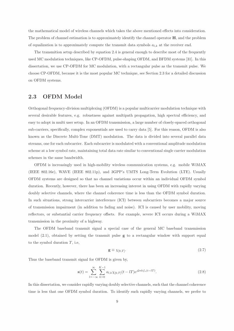
Fig. 2.2 demonstrates a typical OFDM receiver with the ideal channel. The time domain receive

signal is first demodulated from the carrier frequency fc, the cyclic-prefix is removed, and then the

signal is changed to a digital equivalent for further signal processing. The digital time domain baseband

10

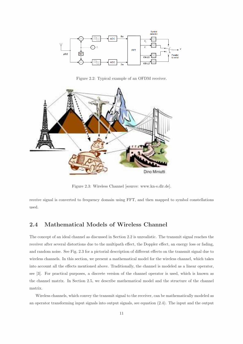
Figure 2.2: Typical example of an OFDM receiver.

Figure 2.3: Wireless Channel [source: www.kn-s.dlr.de].

receive signal is converted to frequency domain using FFT, and then mapped to symbol constellations

used.

2.4 Mathematical Models of Wireless Channel

The concept of an ideal channel as discussed in Section 2.2 is unrealistic. The transmit signal reaches the

receiver after several distortions due to the multipath effect, the Doppler effect, an energy loss or fading,

and random noise. See Fig. 2.3 for a pictorial description of different effects on the transmit signal due to

wireless channels. In this section, we present a mathematical model for the wireless channel, which takes

into account all the effects mentioned above. Traditionally, the channel is modeled as a linear operator,

see [3]. For practical purposes, a discrete version of the channel operator is used, which is known as

the channel matrix. In Section 2.5, we describe mathematical model and the structure of the channel

matrix.

Wireless channels, which convey the transmit signal to the receiver, can be mathematically modeled as

an operator transforming input signals into output signals, see equation (2.4). The input and the output

11

signal of such a system can be described either in time or frequency domain according to convenience.

We first describe a mathematical model for the channel operator, whose input and output are in the

time domain. The physical significance of the variables in the model are also explained.

We consider the mathematical model for the baseband equivalent of the time-domain transmit signal

s, as described in equation (2.1). The mathematical model for the time-domain receive signal r, as

described in equation (2.4), is the effect of the operator H on the time-domain receive signal. In the

following subsections, we develop a mathematical model for the operator H. Throughout the remaining

section, we assume that the maximum delay due to multipath propagation is τmax, and the maximum

Doppler shift due to mobility is νmax. Note, τmax is expressed in units of time, and νmax is expressed in

units of frequency, i.e. the inverse of time.

Multipath Effect

First, we consider channels that have only multipath effects, and no Doppler effects. In such a case, the

receive signal r at time t is the superposition of several instances of the time-domain transmit signal

s with different delays, with a maximum delay of τmax. Thus, the receive signal in this case, and in

absense of any other ambient noise is modeled as

r(t) =

∫ τmax

τ=0

SH(τ)s(t− τ)dτ. (2.12)

Here, SH(τ) is known as the input-delay spreading function, see [3]. SH(τ) can be interpreted as the

attenuation, or gain in the τ -th multipath. Such a channel operator is common, and arises when there

is no mobility between the transmitter and the receiver. For example, in wireless-LAN, there is no

significant mobility between the transmitter and the receiver. Channel estimation and equalization

algorithm for standards IEEE 802.11 a-g are based on such wireless channel models. We notice, that the

receive signal r is a pure convolution of the transmit signal s and the input-delay spread function SH .

Thus the receive signal can also be expressed as

r(t) = SH(τ) ∗ s(t), (2.13)

where ∗ denotes the convolution operator. Applying the Fourier transform on both sides of the equa-

tion (2.13), we get an equivalent expression in the frequency domain as:

r(f) = SH(f)s(f). (2.14)

We note, that the frequency-domain receive signal r is proportional to the frequency-domain transmit

signal s . The proportionality factor SH is known as the frequency attenuation. Thus this type of

channels, which have only the multipath effect, but no Doppler effect, are known as frequency selective

channels.

12

Doppler effect

Mobility between the receiver and the transmitter introduces the Doppler effect in the wireless channel.

In such a case, the time-domain receive signal r is the superposition of several instances of the time-

domain transmit signal s at different delays due to the multipath, and each instance at a specific delay

of the transmit signal in turn is effected by the Doppler effect. Thus, we generalize the wireless channel

model in equation (2.12), for the case where the channel has both, the delay and the Doppler effect, in

the following manner by:

r(t) =

∫ τmax

τ=0

∫ νmax

ν=−νmax

SH(τ, ν)s(t− τ)e2πνtdνdτ, (2.15)

where, SH(τ, ν) is called the delay-Doppler spreading function. Intuitively, this is the factor by which an

instance of the time-domain transmit signal s at the delay τ and with the Doppler effect ν, contributes

to the time-domain receive signal r. Such wireless channels, in which the delay due to the multipath

effect, and the Doppler effect, are both present are known as doubly selective channels.

We notice in equation (2.15) that the time-domain receive signal r is related to the time-domain trans-

mit signal s through a pseudo-differential operator [19]. The product 2τmaxνmax is called the spread of

the operator. If 2τmaxνmax ≪ 1, then the operator defined in equation (2.15) is called an underspread

operator [28]. Underspread operators have several desirable properties, e.g. they are approximately nor-

mal, and therefore have approximately orthogonal eigenfunctions. Such properties are extremely useful

for robust transmission [28]. But in this dissertation, we consider wireless channels with a significant

delay (τmax) and a Doppler effect (νmax), and the underspread assumption is not satisfied in such cases.

The maximum Doppler effect νmax is computed from the relative velocity between the transmitter

and the receiver in the following manner:

νmax =v

cfc, (2.16)

where, v is relative speed between the transmitter and the receiver, fc is the carrier frequency (2.3), and

c is the speed of electromagnetic wave, i.e speed of the light. Another useful measure of the Doppler

effect for multicarrier wireless communication systems is the normalized maximum Doppler, which is

given by the ratio between the maximum Doppler effect and the intercarrier frequency spacing fs, see

equations (2.1) and (2.2). Thus the normalized Doppler is computed as follows:

νnorm =νmax

fs=

v

c

fcfs

. (2.17)

Unaccountable Additive Noise

Other than the multipath effect, and the Doppler effect, there are several minor effects that are unac-

countable, like the magnetic field in the surroundings. The aggregation of all those effects are taken

into account by adding noise to the modeled receive signal. With the additive noise, the model for the

time-domain receive signal is given by

r(t) =

∫ τmax

τ=0

∫ νmax

ν=−νmax

SH(τ, ν)s(t− τ)e2πνtdνdτ + z(t), (2.18)

13

Transmit: time Transmit: Frequency

Receive: time r(t) =∫s(k)K1(t, k)dk r(t) =

∫s(f)K3(t, f)df

Receive: Frequency r(f) =∫s(t)K4(f, t)dt r(f) =

∫s(l)K2(f, l)dl

Table 2.1: Linear integral operators describing wireless channel

where z is a noise process.

The noise process z is characterized by its intensity and distribution. The intensity of the noise is

mostly represented in terms of Signal to Noise Ratio (SNR). SNR is a unit free quantity, which is the

ratio of the signal power to the noise power. Often SNR is expressed in decibel (dB). For a frequency

modulation transmissions scheme, like OFDM, the SNR is often expressed as the ratio of energy per bit

to the noise spectral density (Eb/N0). The distribution of the noise is also dependent on the wireless

environment. The process z being a noise process has its first order moment equal to zero. The second

order cross correlation determines the color of the noise. Generally, the noise is considered to be white,

that is without cross correlation, and in such cases the variance of the distribution is determined by

the SNR. Most of the time, the noise process z(t) is considered to be white Gaussian noise. In this

dissertation, we do not make any assumption about the distribution of the noise process. The proposed

algorithms for channel estimation and equalization are independent of distribution of the noise. Moreover,

the algorithms for channel estimation and equalization that we present in this dissertation do not make

use of any statistical information related to data, channel or noise.

Time Variant System Functions

In fact, the transmit receive relation through the delay-Doppler spreading function, equation (2.18), is

equivalent to a generic time-delay domain relation

r(t) =

∫

τ

h(t, τ)s(t− τ)dτ + z(t). (2.19)

where,

h(t, τ) =

∫

ν

SH(τ, ν)e2πνtdν. (2.20)

h(t, τ) is known as the channel impulse response. We drop the limits of the integration as they are

evident. The function h(·, τ) is called the channel tap at the τ -th delay, and it is denoted by hτ for

convenience.

The inputs and the outputs of the wireless channel may be described in either the time or frequency

domain. Since either the time or the frequency domain can be used, the channel is described by any of

the four operators shown in Table 2.1. We notice that the kernel K1 in Table 2.1 is the channel impulse

14

response h(t, τ) (2.19). The relations between the kernels K1, K2, K3, K4 of the the linear time variant

systems describing wireless channels are presented in [3], [52].

WSSUS

Wireless channels are also characterized from the statistical point of view, see [3] for detail. In such

approaches, the kernels K1, K2, K3, K4 are considered stochastic process, and their second order

statistics are used to characterize the time varying system functions.

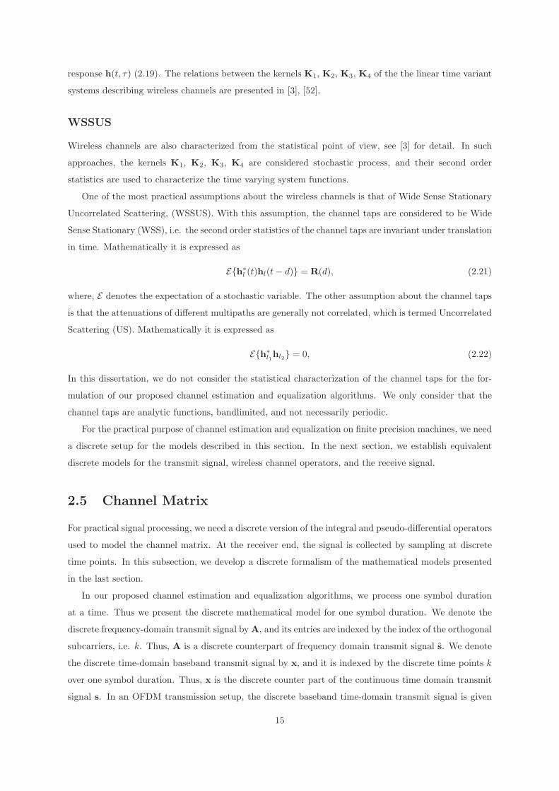
One of the most practical assumptions about the wireless channels is that of Wide Sense Stationary

Uncorrelated Scattering, (WSSUS). With this assumption, the channel taps are considered to be Wide

Sense Stationary (WSS), i.e. the second order statistics of the channel taps are invariant under translation

in time. Mathematically it is expressed as

E{h∗

l (t)hl(t− d)} = R(d), (2.21)

where, E denotes the expectation of a stochastic variable. The other assumption about the channel taps

is that the attenuations of different multipaths are generally not correlated, which is termed Uncorrelated

Scattering (US). Mathematically it is expressed as

E{h∗

l1hl2} = 0, (2.22)

In this dissertation, we do not consider the statistical characterization of the channel taps for the for-

mulation of our proposed channel estimation and equalization algorithms. We only consider that the

channel taps are analytic functions, bandlimited, and not necessarily periodic.

For the practical purpose of channel estimation and equalization on finite precision machines, we need

a discrete setup for the models described in this section. In the next section, we establish equivalent

discrete models for the transmit signal, wireless channel operators, and the receive signal.

2.5 Channel Matrix

For practical signal processing, we need a discrete version of the integral and pseudo-differential operators

used to model the channel matrix. At the receiver end, the signal is collected by sampling at discrete

time points. In this subsection, we develop a discrete formalism of the mathematical models presented

in the last section.

In our proposed channel estimation and equalization algorithms, we process one symbol duration

at a time. Thus we present the discrete mathematical model for one symbol duration. We denote the

discrete frequency-domain transmit signal byA, and its entries are indexed by the index of the orthogonal

subcarriers, i.e. k. Thus, A is a discrete counterpart of frequency domain transmit signal s. We denote

the discrete time-domain baseband transmit signal by x, and it is indexed by the discrete time points k

over one symbol duration. Thus, x is the discrete counter part of the continuous time domain transmit

signal s. In an OFDM transmission setup, the discrete baseband time-domain transmit signal is given

15

by inverse discrete Fourier transform of the discrete frequency-domain signal, see equation (2.10), and if

a cyclic prefix is used then see equation (2.11). The inverse discrete Fourier transform is performed by

IFFT algorithms, which is a O(K logK) algorithm, where K is the total number of subcarriers.

We denote the discrete time-domain receive signal by y, and it is indexed by the sampling index n.

Thus, y is a discrete counterpart of the time-domain receive signal r. We consider that the transmission

and the reception synchronized by a known time lag, so we can safely assume the same index k for the

signal samples at the transmitter and the receiver. We denote the discrete frequency-domain receive

signal by Y , and it is indexed by k.

We denote the discrete time-domain channel matrix by H. The rows and the columns are indexed

by the sampling index k. Thus the time-domain transmit-receive signal relation in the discrete setup is

given by

y = Hx+w, (2.23)

where w is the discrete time domain noise process. Applying the Discrete Fourier Transform (DFT)

operator F on either side of equation (2.23), we get the discrete frequency-domain transmit receive

relation as

Y = HA+W, (2.24)

where, H = FHF ∗ is the frequency domain channel matrix.

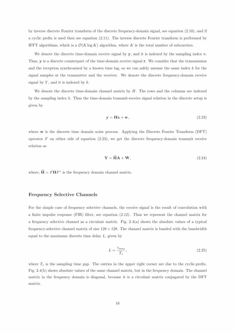
Frequency Selective Channels

For the simple case of frequency selective channels, the receive signal is the result of convolution with

a finite impulse response (FIR) filter, see equation (2.12). Thus we represent the channel matrix for

a frequency selective channel as a circulant matrix. Fig. 2.4(a) shows the absolute values of a typical

frequency-selective channel matrix of size 128× 128. The channel matrix is banded with the bandwidth

equal to the maximum discrete time delay L, given by

L =τmax

Ts

, (2.25)

where Ts is the sampling time gap. The entries in the upper right corner are due to the cyclic-prefix.

Fig. 2.4(b) shows absolute values of the same channel matrix, but in the frequency domain. The channel

matrix in the frequency domain is diagonal, because it is a circulant matrix conjugated by the DFT

matrix.

16

(a) In the time domain (b) In the frequency domain

Figure 2.4: The support of a frequency selective channel matrix.

H =

h1 0 . . . 0 hτmax hτmax−1 hτmax−2 . . . h2

h2 h1

. . . 0 0 hτmax hτmax−1 . . . h3

h3 h2 h1

. . .. . . 0 hτmax . . . h4

.

.

.

.

.

.. . .

. . .. . .

. . .. . .

. . ....

.

.

.

.

.

.. . .

. . .. . .

. . .. . .

. . ....

0 0 . . . hτmax hτmax−1 hτmax−2 hτmax−3 . . . h1

Doubly Selective Channels

For the general case of doubly-selective channels, which occur due to the multipath delay and the Doppler

effect, the wireless channel act like a time-varying filter. That is, an FIR in which the filter coefficients are

changing with time. Fig. 2.5(a) shows the absolute value of a matrix in the time domain which represents

a time-varying FIR. This doubly-selective wireless channel is simulated for a normalized Doppler of 18%.

The matrix is banded, and the bandwidth is determined by the maximum discrete time delay L. The

17

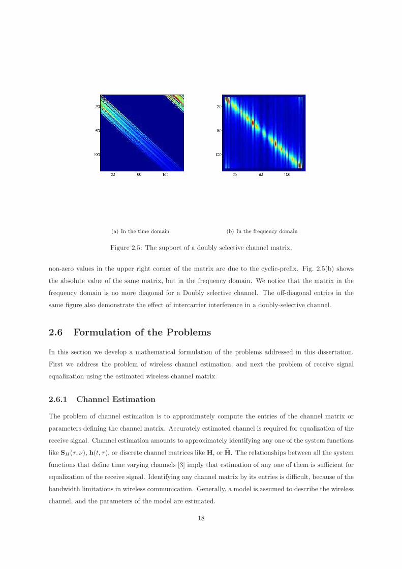
(a) In the time domain (b) In the frequency domain

Figure 2.5: The support of a doubly selective channel matrix.

non-zero values in the upper right corner of the matrix are due to the cyclic-prefix. Fig. 2.5(b) shows

the absolute value of the same matrix, but in the frequency domain. We notice that the matrix in the

frequency domain is no more diagonal for a Doubly selective channel. The off-diagonal entries in the

same figure also demonstrate the effect of intercarrier interference in a doubly-selective channel.

2.6 Formulation of the Problems

In this section we develop a mathematical formulation of the problems addressed in this dissertation.

First we address the problem of wireless channel estimation, and next the problem of receive signal

equalization using the estimated wireless channel matrix.

2.6.1 Channel Estimation

The problem of channel estimation is to approximately compute the entries of the channel matrix or

parameters defining the channel matrix. Accurately estimated channel is required for equalization of the

receive signal. Channel estimation amounts to approximately identifying any one of the system functions

like SH(τ, ν), h(t, τ), or discrete channel matrices like H, or H. The relationships between all the system

functions that define time varying channels [3] imply that estimation of any one of them is sufficient for

equalization of the receive signal. Identifying any channel matrix by its entries is difficult, because of the

bandwidth limitations in wireless communication. Generally, a model is assumed to describe the wireless

channel, and the parameters of the model are estimated.

18

For frequency-selective channels, the channel matrix H is determined by L FIR filter coefficients.

Thus the channel estimation amounts to approximate computation of the filter coefficients. Moreover,

for frequency selective channels, the channel matrix in the frequency domain H is diagonal. Thus another

approach for channel estimation is to estimate the diagonal elements of H. Generally, in this approach,

a few of the diagonal elements of H are computed using pilot information, and the remaining diagonal

elements are approximated by interpolation.

For doubly-selective channels, a popular approach is to model the channel taps hl as combination

of suitable basis functions, see [49, 15, 54, 45]. This approach is known as the the Basis Expansion

Model (BEM). With a BEM wireless channel estimation amounts to approximate computation of the

coefficients in the expansion of the channel tap as linear combination of the known basis functions.

Wireless channel estimation is done in two ways, blind estimation and pilot-aided estimation. Pilot

aided estimation usually employs some subcarriers with known values while transmitting the signal.

That is, some of the values of the discrete frequency domain transmit signal A are set with known values

before modulation (2.10). These reserved subcarriers are known as the pilot carriers, and the values of

the pilot carriers are known as the pilot values. At the receiver end, the pilot information is used to

estimate the channel. The other type of estimation, which does not use pilot information, is known as

blind channel estimation. In this dissertation, we only focus on pilot-aided estimation methods.

In this dissertation, notation of every estimated object will be distinguished from the exact object

with a tilde (·) above the symbol of the exact object. For example, the discrete frequency domain

transmit signal is denoted by A, and the estimated discrete frequency domain transmit signal is denoted

by A.

In Chapter 3 we present some of the classical and contemporary channel estimation algorithms. In

Chapter 4 we present a novel channel estimation algorithm for doubly-selective channels using a Basis

Expansion Model.

2.6.2 Equalization

The signal received at the receiver end is the effect of the wireless channel and added noise, see equa-

tion (2.23) and equation (2.24). The purpose of equalization is to recover the time-domain transmit

signal x, or the frequency-domain transmit signal A from the receive signal y, and the estimated wire-

less channel. An OFDM-type system transmits by modulating data with discrete orthogonal frequencies.

Before modulation, the information bits are first mapped to a fixed constellation (alphabet), like 4QAM,

QPSK. In practice, data bits are encoded with an error correcting code before transmitting. They are

later decoded after the signal is equalized at the receiver end.

For a time invariant frequency selective channel, the channel matrix in the frequency domain H is

diagonal. The entries of the diagonal matrix H are called the frequency attenuations. In this setup,

equalization is best done by pointwise division of the receive signal by the corresponding frequency

attenuation. This method of equalization is known as single-tap (ST) equalization. In the presence

19

of added noise in the system, ST equalization is optimal in the least squares sense for time invariant

frequency selective channels.

For time varying doubly selective channels, the frequency domain channel matrix H is no more

diagonal, which causes ICI during equalization. Equalization for such a wireless channel is difficult, and

we address this problem in this dissertation. Even if the exact channel matrix H is known, the added

noise in the receive signal y makes equalization difficult. Moreover, commercial hardware devices expect

equalization to be done in a very short time, which prevents us from using O(K3) algorithms for solving

linear systems. In Chapter 5 we propose a fast algorithm for regularized equalization.

In Chapter 3 we present some of the classical and recent equalization methods for the OFDM setup.

In Chapter 5 we present a novel equalization algorithm for doubly-selective wireless channels using a Basis

Expansion Model. The proposed method has several desirable features, for example, it uses the estimated

BEM coefficients directly, without ever creating the channel matrix, and computes a regularized solution.

2.7 Related Mathematical Research Areas

In this section, we discuss mathematical research areas related to the problems we are addressing in

this dissertation. There are several mathematical research areas related to the problems of channel

estimation and equalization, we mention some of them, which we use heavily in solving the problems

in this dissertation. Specifically, we discuss a resolution of the Gibbs phenomenon in Subsection 2.7.1,

solution of linear systems in Subsection 2.7.2, and low precision numerical methods in Subsection 2.7.5.

At the end, Subsection 2.7.6, we provide an short overview of other related research areas.

2.7.1 Resolution of the Gibbs Phenomenon

Pilot assisted methods are already available for computation of the Fourier coefficients of the channel

taps hl of doubly selective channels [45, 29, 21]. In Chapter 4, we propose a fast and accurate algorithm

for estimation of the Fourier coefficients of the channel taps. The channel taps are generally non-periodic

analytic functions. Reconstruction of channel taps with the estimated Fourier coefficients are inadequate

because of the Gibbs phenomenon.

As stated in [17], ”The inability to recover point values of a nonperiodic, but otherwise perfectly

smooth, function from its Fourier coefficients is the Gibbs phenomenon”. There are several methods for

mitigating the Gibbs phenomenon, see [17] for a detailed survey. Most of the methods can be classified

either as filtering in the frequency domain or as projection in the time domain. In our work we use

a projection in the time domain approach to resolve the Gibbs phenomenon. In our problems, the

number of Fourier coefficients available is very small, limited by the number of pilot carriers. In such a

case projection of trigonometric polynomials on Gegenbauer polynomials is a very effective method for

resolving the Gibbs phenomenon, see [17].

20

2.7.2 Solution of Linear Systems

The theory of linear systems is a branch of linear algebra, see [16], [11], [48], a subject which is funda-

mental to modern mathematics. Computational algorithms for finding the solutions are an important

part of numerical linear algebra, and such methods play a prominent role in engineering, physics, chem-

istry, computer science, and economics. Let us consider the linear system derived from the time-domain

transmit-receive relation (2.23) by ignoring the noise component,

Hx = y. (2.27)

Thus matrix H is of size K ×K, and x, y are vectors of length K. Solution of the linear system (2.27)

amounts to finding x given the K × K matrix H and the vector y of size K. This is a formulation

of a square system system, where there is K unknowns and K equations. Linear systems with more

equations than unknowns are known as overdetermined systems. Linear systems with fewer equations

than unknowns are known as underdetermined systems. For problems addressed in this dissertation, we

mostly need square systems.

There are several algorithms available for solution of the linear system given by the equation 2.27,

see [16]. Depending on sparsity and structure of the matrix H, several algorithms can be employed for

finding the solution x. Most of the algorithms are categorized into two main types, direct and iterative.

Direct methods include solution by Gaussian elimination, which uses the LU decomposition of the matrix

H. A stable solution is achieved by using a LU decomposition of H with partial pivoting or complete

pivoting. Similarly, the solution x can be found by the QR factorization of H. A completely different

approach is often taken for very large systems. The idea is to start with an initial approximation to the

solution, and to change this approximation in several steps to bring it closer to the true solution. Once

the approximation is sufficiently accurate, this is taken to be the solution to the system. This leads to

the class of iterative methods. Examples of iterative methods are GMRES, LSQR, CG etc..

The linear systems that we address in this dissertation are of size 256× 256, 512× 512, 1024× 1024,

or even larger. The solution is required to be computed in real time of around 100µs or less. Thus we

cannot employ direct methods which use O(K3) operations. We use iterative methods for our purpose.

In the next section, we describe Krylov subspace based iterative methods.

2.7.3 Krylov Subspace Based Methods

The order-i Krylov subspace generated by a K×K matrix H and a vector y of dimension K is the linear

subspace spanned by the images of y under the first i powers of H (starting from H0 = I), that is,

K(H,y, i) = span {y,Hy,H2y, . . . ,Hi−1y}. (2.28)

In a Krylov subspace based method for solution of a linear system, each approximate solution of x is

sought within an increasing family of Krylov subspaces. In this dissertation, we use two most commonly

used Krylov subspace based method for solution of linear systems, namely GMRES [39] and LSQR [34].

21

At the ith iteration, GMRES constructs an approximation within the subspace

K(H,y, i) = Span{y,Hy,H2y, . . . ,H(i−1)y

}, (2.29)

whereas LSQR within the subspace

K(HHH,HHy, i) = Span{HHy, (HHH)HHy, . . . , (HHH)(i−1)HHy

}. (2.30)

These methods use the number of iterations as a regularization parameter. In next the two paragraphs,

we give a detailed description of GMRES [39] and LSQR [34]. We consider the linear system presented

in equation (2.27).

GMRES

GMRES approximates the exact solution of (2.27) by the vector xi ∈ K (H,y, i) that minimizes the norm

‖ri‖2 of the residual

ri = Hxi − y. (2.31)

The vectors y,Hy, . . . ,H(i−1)y are not necessarily orthogonal, so the Arnoldi iteration is used to

find orthonormal basis vectors q1,q2, . . . ,qi for K (H,y, i). Subsequently, the vector xi ∈ K (H,y, i) is

written as xi = Qibi, where Qi is the K × i matrix formed by q1, . . . ,qi, and bi ∈ Ci.

The Arnoldi process also produces an (i+ 1)× i upper Hessenberg matrix Hi which satisfies

HQi = Q(i+1)Hi. (2.32)

Because Qi has orthogonal columns, we have

‖Hxi − y‖2 = ‖Hibn − βe1‖2, (2.33)

where e1 = (1, 0, 0, . . . , 0), and β = ‖y‖2.

Therefore, xi can be found by minimizing the norm of the residual

rn = βe1 −Hibi. (2.34)

This is a linear least squares problem of size i, which is solved by using the QR factorization. One can

summarize the GMRES method as follows.

At every step of the iteration:

1. Do one step of the Arnoldi method.

2. Find the bi which minimizes ‖ri‖2 using the QR factorization at a cost of O(i2) flops.

3. Compute xi = Qibi.

4. Repeat if the residual is not yet small enough.

22

LSQR

LSQR is an iterative algorithm for the approximate solution of the linear system (2.27). In exact arith-

metic, LSQR is equivalent to the conjugate gradient method for the normal equations HHHx = HHy.

Specifically, at the ith iteration, one constructs a vector xi in the Krylov subspace K(HHH,HHy, i

)

that minimizes the norm of the residual ‖Hxi − y‖2.LSQR repeats two steps: the Golub-Kahan bidiagonalization and the solution of a bidiagonal least

squares problem. The Golub-Kahan bidiagonalization [16] constructs vectors ui, vi, and positive con-

stants αi, βi (i = 1, 2, . . .) as follows:

1. Set β1 = ‖y‖2, u1 = y/β1, α1 = ‖HHy‖2, v1 = HHy/α1.

2. For i = 1, 2, . . ., set

βi+1 = ‖Hvi − αiui‖2, ui+1 = (Hvi − αiui)/βi+1,

αi+1 = ‖HHui − βivi‖2, vi+1 = (HHui − βivi)/αi+1.

The process is terminated if αi+1 = 0 or βi+1 = 0.

In exact arithmetic, the ui’s are orthonormal, and so are the vi’s. Therefore, one can reduce the

approximation problem over the ith Krylov subspace to the following least square problem:

minwi

‖Biwi − [β1, 0, 0, . . .]T ‖2, (2.35)

whereBi is the (i+1)×i lower bidiagonal matrix with α1, . . . , αi on the main diagonal, and β2, . . . , βi+1 on

the first subdiagonal. This least squares problem is solved at a negligible cost using the QR factorization

of the bidiagonal matrix Bi. Finally, the ith approximate solution is computed as

xi =i∑

j=1

wi(j)vj . (2.36)

The second LSQR step solves the least squares problem (2.35) using the QR factorization of Bi. The

computational costs of this step are negligible due to the bidiagonal nature of Bi. Furthermore, [34]

introduced a simple recursion to compute wi and xi via a simple vector update from the approximate

solution obtained in the previous iteration.

2.7.4 Preconditioning

Preconditioners are used to accelerate convergence of iterative solvers by replacing a given matrix with

one that has closely clustered eigenvalues, see [16], section 10.3. An approximate inverse of the matrix

is commonly used as a preconditioner, resulting in the eigenvalues clustered around the point z = 1 in

the complex plane. Algebraically, there are two types of preconditioners, namely a left preconditioner,

and right preconditioner.

A right preconditioner PR of the linear system in equation 2.27, is used in the following manner:

HPRP−1R x = y (2.37)

Hx = y, (2.38)

23

where H = HPR, x = P−1R x. First equation (2.38) is solved for x, and then we set:

x = P−1R x. (2.39)

Similarly, a left preconditioner PL of the linear system in equation 2.27, is used in the following

manner:

PLHx = PLy (2.40)

Hx = y. (2.41)

Equation (2.41) is solved for x.

One commonly used preconditioner for linear systems is the Jacobi preconditioner. The classical

Jacobi method uses the diagonal of a matrix H to form a diagonal preconditioner. Other commonly used

preconditioner uses an incomplete LU factorization and incomplete Cholesky factorization, see [16] for

more details. In Chapter 5 we introduce a preconditioner suitable for wireless channels modeled using a

BEM.

2.7.5 Effective Numerical Precision

Wireless communications receive signals always have unaccountable additive noise. Such noise arises due

to several factors, e.g., inaccuracies in the measurement, unknown magnetic fields in the surroundings.

Inaccuracy in modeling of the wireless channel also contributes to noise. Generally, the Signal to Noise

Ratio (SNR) of the receive signal is around 15 dB, i.e. the ratio between the power of the signal to

the power of the noise is around 30. Thus on an average, the 5th bit of receive signal is unreliable and

corrupted by noise. With certain probability, depending on the actual distribution of the noise, the 4th

and the 3rd bit of the receive signal may also be corrupted due to noise. Thus effectively the precision

of the receive signal is not determined by the width of the register used to store the sampled receive

signal, rather it is determined by the level of noise. Thus the precision of the receive signal is very low,

only few correct bits are available for further signal processing. Numerical methods which are suitable

for computing with full or double precisions, conforming with conventional IEEE 754 standard, might

not work properly with signals with noise.

The transmit information are quantized using certain alphabets, e.g. 4QAM, BPSK etc.. For ex-

ample, if 4QAM is used to quantize the transmit signal, then to recover the transmit information at

the receiver end, we only need to recover the first bit correctly (using the two’s complement, big-endian

representation). Getting the first significant bit correct from the noisy receive signal is a challenge,

because in the receive signal only very few correct bits are available. To deal with noisy receive signal,

we always try to keep the condition number of the pertinent linear operators as small as possible, and

try to use regularized methods whenever possible. For example, an operation with condition number of

100 = O(26) is not desirable, because such operator likely corrupts the first significant bit if applied to

a signal with SNR of 15dB.

24

2.7.6 Other Related Research

In this dissertation, we focus on two main problems related to wireless communications, i.e. wireless

channel estimation and equalization. There are other research areas which address the problems related

to fast and reliable wireless communications systems. In this subsection, we present a very concise

overview of two such related research areas, namely modeling of wireless channels, and error correcting

codes.

Modeling of Wireless Channels

Modeling of wireless channels is a fundamental task for wireless channel estimation and equalization.

Proper modeling of wireless channels is required for computer simulations, which are further used for

testing algorithms for wireless channel estimation and equalization. In [3, 4], one can find a detailed

treatment on modeling of wireless channels, their characterization in the time and the frequency domains,

and also their representations as stochastic processes with certain characteristics. Detailed algorithms

for simulation of wireless channels with certain characteristics can be found in [25], and [40].

Forward Error Correction

In telecommunication and information theory, forward error correction (FEC) is a system of error control

for data transmission, whereby the sender adds redundant data to its messages, FEC is also known as

an error correction code. For example, the redundancy with factor 2 is called 1/2-FEC, or FEC with

code rate 1/2. This allows the receiver to detect and correct errors to a certain degree without the need

to ask the sender for additional data. The advantage of forward error correction is that a request for

retransmission is not required at the cost of higher bandwidth. FEC is therefore applied in situations

where retransmissions are relatively costly or impossible, like digital video broadcasting. Generally,

FEC circuits are often an integral part of the analog-to-digital conversion process, also involving digital

modulation and demodulation, e.g. IEEE 802.11 a-g. There are several ways of doing forward error

correction. The most popular are convolution coding, Reed-Solomon coding, low-density parity check

coding etc..

At the receiver, the decoding is done, using the parameters (known as codes) used for FEC. The

maximum fraction of errors that can be corrected is determined in advance by the design of the code, so

different forward error correcting codes are suitable for different conditions. Detection depends on the

algorithm used for decoding. The two most frequently used decoding algorithms are the BCJR algorithm

[2] and the Viterbi algorithm [50].

Turbocoding is a scheme that combines two or more relatively simple convolutional codes and an

interleaver to produce a block code that can perform to within a fraction of a decibel of the Shannon

limit. In this dissertation, we used turbo coding as FEC. The reported BERs are after decoding with

the BCJR algorithm. We use turbocoding parameters conforming to the standard IEEE 802.16e.

25

2.8 Measurements of Transmission Quality

For testing and comparing quality of wireless channel estimation and equalization methods, several

measures are available. The most common among them are Symbol Error Rate (SER), Bit Error Rate

(BER), and Normalized Mean Square Error (NMSE).

The SER is the ratio of the number of incorrect symbols (QPSK, 4QAM) received to the number

of transmitted symbols. The BER is the fraction of the number of incorrect bits received compared

to the number of all transmitted bits. Generally, the BER is measured whenever an error correcting

code is used. The SER and the BER are used mainly to measure the quality of equalization algorithms.

Obviously, they also reflect the performance of the wireless channel estimation used in conjunction with

the equalization algorithm. To assess the quality of equalization methods independently of the channel

estimation algorithm, the exact wireless channel is used for equalization. This is only possible in a

computer simulation study. The NMSE is used for measuring the quality of the estimation only. The

NMSE is computed as the power of the error in estimating wireless channel tap compared to the total

power of the channel taps. Typically, the NMSE is expressed in decibels. Computation of NMSE is only

possible in a computer simulation study.

In this dissertation, we use both the BER and the NMSE to measure the quality of wireless channel

estimation and equalization methods.

26

Chapter 3

Channel Estimation and

Equalization: Classical and

Contemporary Algorithms

3.1 Introduction

In this chapter, we discuss presently available algorithms for wireless channel estimation and equalization

with OFDM systems. Some of these algorithms are used for OFDM based wireless devices, like WLAN

(wireless local area network). First, we discuss channel estimation algorithms, and then equalization

algorithms. We discuss only pilot-aided algorithms that do not use any statistical information about

channel, data or noise.

3.2 Channel Estimation

As discussed in Chapter 2, wireless channel estimation amounts to approximate computation of the

entries of the wireless channel matrix, or approximate computation of certain parameters that describe

the wireless channel. We consider the transmit-receive signal relation in the time domain as derived in

the equation (2.23):

y = Hx+w, (3.1)

where y is the time-domain receive signal, H is the time-domain channel matrix, x is the time-domain

transmit signal, and w is an additive noise process. In an OFDM based transmission, the time-domain

transmit signal is generated from the frequency-domain transmit signal A using an inverse discrete

Fourier transform, see equation (2.10) and equation (2.11). Pilot aided channel estimation methods

employ some part of the frequency-domain transmit signal A for transmitting pilot information, and the

remaining part is used for data transmission. That is certain OFDM subcarriers are used to transmit

27

pilot information, and rest of the subcarriers are used to transmit data. The pilot information is known

at the receiver, and the receiver uses the pilot information to approximately compute the channel matrix.

3.3 Frequency Selective Channel

In wireless communications systems, the transmitted signal typically propagates via several different

paths from the transmitter to the receiver. This is caused by reflections of the electromagnetic radio waves

from the surrounding buildings or other obstacles, and is commonly known as multipath propagation.

Each multipath component of the electromagnetic wave has a different relative propagation delay and

path loss. At the receiver, the multipath effect results in a filtering effect on the transmit signal. In the

frequency domain, different frequencies of the modulated waveform experience different attenuations and

phase changes. Such wireless channels are known as frequency-selective channels. On the other hand,

wireless channels with frequency-selective fading and Doppler effect due to transmitter-receiver mobility

are much more complex. They are known as doubly-selective channels, see Section 3.7 for detail.

We consider the time-domain transmit-receive relation as in equation (3.1). For a frequency-selective

wireless channel, the time-domain channel matrix H represents a time-invariant finite impulse response

(FIR) filter. Equivalently, H is a circulant matrix, with non-zero entries on a band at and below the

diagonal and on a triangular region at the upper right corner of the matrix. The non-zero entries on a

rectangular region at the upper right corner of the matrix represents the cyclic nature of the FIR, which

is achieved using cyclic prefix at the transmission. The frequency-domain transmit-receive relation is

derived from the time-domain transmit-receive relation by applying the discrete Fourier transform on

both sides of the equation (3.1)

Fy = FHF∗Fx+ Fw (3.2)

Y = DA+W, (3.3)

where F denotes the discrete Fourier transform operator, and D denotes the frequency domain channel

matrix. Evidently, for a frequency-selective channel, the frequency-domain channel matrix D is diagonal.

The ith diagonal entry of the matrix D is generally called the frequency attenuation at the ith subcarrier.

Channel estimation for frequency-selective channels is done both in the time domain and in the

frequency domain. In the time domain, channel estimation amounts to identifying the filter coefficients,

that forms the circulant matrixH, see Section 3.6 for details. In the frequency domain, channel estimation

amounts to identifying the diagonal entries of the matrix D, see Section 3.5 for more details.

3.4 Pilot Arrangement

For rapidly-varying channels, pilot assisted channel estimation methods are popular and reliable. For

a pilot assisted channel estimation method for OFDM systems, arrangement of the pilot subcarriers

and their values is crucial for the overall performance. The subcarriers transmitting pilot information

28

g

g

g

g

g

g

g

g

g

g

g

g

g

g

g

g

g

g

g

g

g

g

g

g

g

g

g

g

g

g

g

g

g

g

g

g

g

g

g

g

g

g

g

g

g

g

g

g

g

g

g

g

g

g

g

g

g

g

g

g

g

g

g

g

g

g

g

g

g

g

g

g

g

g

g

g

g

g

g

g

g

g

g

g

g

g

g

g

g

g

g

g

g

g

g

g

g

g

g

g

g

g

g

g

g

g

g

g

g

g

g

g

g

g

g

g

g

g

g

g

g

g

g

g

g

g

g

g

w

w

w

w

w

w

w

w

w

w

w

w

w

w

w

w

w

w

w

w

w

w

w

w

w

w

w

w

w

w

w

w

6

-

N

◮

Symbols

Subcarriers

Figure 3.1: An illustration of the block-type pilot arrangement with K = 16 subcarriers (’◦’ representsdata symbols and ’•’ represents pilot symbols).

are often called pilot tones. The pilot information is used at the receiver end to estimate the wireless

channels. By pilot information, we mean the position of the pilot subcarriers, and the values which

modulate those subcarriers. Increasing the number of pilot tones improves estimation of the wireless

channel, but the final throughput of the system decreases. In this section, we describe different pilot

arrangements that are used in practice.

Block-Type

A block-type pilot arrangement requires inserting pilot tones into all of the subcarriers of a specific OFDM

symbol. Remaining OFDM symbols are used for data transmission. Fig. 3.1 illustrates a pilot tones

arrangement over OFDM subcarriers and OFDM symbols for a block type pilot arrangement. Block-

type pilot channel estimation has been developed under the assumption of a slowly varying channel. In

addition to the block-type pilot, a decision feedback equalizer is generally used in practice to boost the

performance of the system. WLAN, which conforms to the standard IEEE 802.11a, uses a block type

pilot arrangement for channel estimation.

Comb-Type

A comb-type pilot arrangement requires inserting pilot tones into all OFDM symbols. With a comb-type

pilot arrangement, some of the subcarriers of an OFDM symbol are pilot tones, and the remaining ones

are data carriers. Fig. 3.2 illustrates a typical pilot arrangement over OFDM subcarriers and OFDM

symbols for a comb type pilot arrangement.

The comb-type pilot channel estimation has been introduced to satisfy the need for equalizing when

the channel changes withing one OFDM block. Channel estimation algorithms that uses a comb-type

pilot arrangement estimates the frequency attenuation at pilot subcarriers and then interpolate the

estimated values of the attennuations over the data carrying frequencies. WLAN, which conforms to the

standard IEEE 802.11g, uses a comb type pilot arrangement for channel estimation.

29

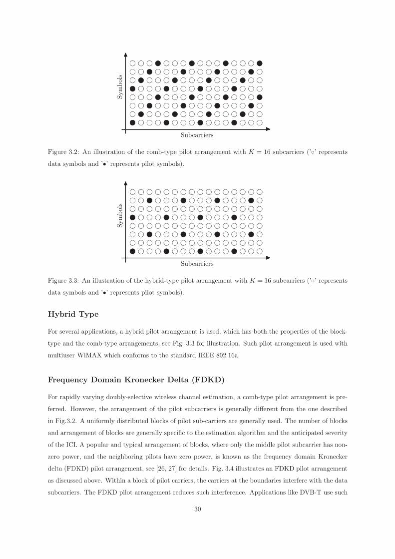
g

g

g

g

g

g

g

g

g

g

g

g

g

g

g

g

g

g

g

g

g

g

g

g

g

g

g

g

g

g

g

g

g

g

g

g

g

g

g

g

g

g

g

g

g

g

g

g

g

g

g

g

g

g

g

g

g

g

g

g

g

g

g

g

g

g

g

g

g

g

g

g

g

g

g

g

g

g

g

g

g

g

g

g

g

g

g

g

g

g

g

g

g

g

g

g

g

g

g

g

g

g

g

g

g

g

g

g

g

g

g

g

g

g

g

g

g

g

g

g

g

g

g

g

g

g

g

g

w

w

w

w

w

w

w

w

w

w

w

w

w

w

w

w

w

w

w

w

w

w

w

w

w

w

w

w

w

w

w

w6

-

N

◮

Symbols

Subcarriers

Figure 3.2: An illustration of the comb-type pilot arrangement with K = 16 subcarriers (’◦’ representsdata symbols and ’•’ represents pilot symbols).

g

g

g

g

g

g

g

g

g

g

g

g

g

g

g

g

g

g

g

g

g

g

g

g

g

g

g

g

g

g

g

g

g

g

g

g

g

g

g

g

g

g

g

g

g

g

g

g

g

g

g

g

g

g

g

g

g

g

g

g

g

g

g

g

g

g

g

g

g

g

g

g

g

g

g

g

g

g

g

g

g

g

g

g

g

g

g

g

g

g

g

g

g

g

g

g

g

g

g

g

g

g

g

g

g

g

g

g

g

g

g

g

g

g

g

g

g

g

g

g

g

g

g

g

g

g

g

g

w

w

w

w

w

w

w

w

w

w

w

w

w

w

w

w

6

-

N

◮

Symbols

Subcarriers

Figure 3.3: An illustration of the hybrid-type pilot arrangement with K = 16 subcarriers (’◦’ representsdata symbols and ’•’ represents pilot symbols).

Hybrid Type

For several applications, a hybrid pilot arrangement is used, which has both the properties of the block-

type and the comb-type arrangements, see Fig. 3.3 for illustration. Such pilot arrangement is used with

multiuser WiMAX which conforms to the standard IEEE 802.16a.

Frequency Domain Kronecker Delta (FDKD)

For rapidly varying doubly-selective wireless channel estimation, a comb-type pilot arrangement is pre-

ferred. However, the arrangement of the pilot subcarriers is generally different from the one described

in Fig.3.2. A uniformly distributed blocks of pilot sub-carriers are generally used. The number of blocks

and arrangement of blocks are generally specific to the estimation algorithm and the anticipated severity

of the ICI. A popular and typical arrangement of blocks, where only the middle pilot subcarrier has non-

zero power, and the neighboring pilots have zero power, is known as the frequency domain Kronecker

delta (FDKD) pilot arrangement, see [26, 27] for details. Fig. 3.4 illustrates an FDKD pilot arrangement

as discussed above. Within a block of pilot carriers, the carriers at the boundaries interfere with the data

subcarriers. The FDKD pilot arrangement reduces such interference. Applications like DVB-T use such

30

g

g

g

g

g

g

g

g

g

g

g

g

g

g

g

g

g

g

g

g

g

g

g

g

g

g

g

g

g

g

g

g

g

g

g

g

g

g

g

g

g

g

g

g

g

g

g

g

g

g

g

g

g

g

g

g

g

g

g

g

g

g

g

g

g

g

g

g

g

g

g

g

g

g

g

g

g

g

g

g

g

g

g

g

g

g

g

g

g

g

g

g

g

g

g

g

g

g

g

g

g

g

g

g

g

g

g

g

g

g

g

g

g

g

g

g

g

g

g

g

g

g

g

g

g

g

g

g

w

w

w

w

w

w

w

w

w

w

w

w

w

w

w

w

w

w

w

w

w

w

w

w

w

w

w

w

w

w

w

w

w

w

w

w

w

w

w

w

w

w

w

w

w

w

w

w6

-

N

◮

Tim

e

Frequency

Figure 3.4: An illustration of the pilot arrangement for doubly selective channels with K = 16, (’◦’represents data symbols and ’•’ represents pilot symbols). For FDKD pilot arrangement, only the

central pilot in each block is non-zero.

a pilot arrangement for channel estimation. An optimal distribution of power between the pilot and the

data subcarriers is still an open problem.

3.5 Frequency Domain Channel Estimation

In this section, we investigate frequency-selective wireless channel estimation in the frequency domain.

Further details of pilot assisted estimation of frequency-selective channels can be found in [10]. The

frequency-selective wireless channel matrix are diagonal in the frequency domain, see equation (3.3).

Estimation With Block Type Pilot Arrangement

In block-type pilot-based wireless channel estimation, OFDM pilot symbols are transmitted periodically,

in which all subcarriers are used as pilots. If the wireless channel is constant across the block, i.e. the

duration of transmission between two pilot symbols, then there is no channel estimation error. Channel

estimation can be performed by using either the least squares (LS) approach, or the minimum mean

square approach (MMSE), see [23, 10, 13].

The MMSE based channel estimation requires the second order statistical information about the

channel and the transmitted data. We do not explain MMSE based estimation method any further, see

[10, 13] for details.

The LS estimation of the frequency domain channel matrix D at pilot symbols is given by

D(k, k) =Y(k)

Pk

, k = 1, . . . ,K. (3.4)

We assume here that the kth subcarrier of the pilot symbol is modulated with a pilot value Pk.

When the channel is slowly varying, channel estimation inside the block can be updated using a

decision feedback equalizer at each sub-carrier. Decision feedback equalizer for the kth subcarrier is

described as follows:

31

• The channel attenuation at the kth subcarrier estimated from the previous OFDM symbol D(k, k)

is used to find (equalize) the frequency domain transmitted signal at the kth subcarrier, i.e. A(k)

in the following way:

A(k) =Y(k)

D(k, k), k = 1, . . . ,K. (3.5)

• A(k) are mapped to the alphabets used, i.e. 4QAM, PSK, etc., as Apure(k).

• The estimated channel attenuation at the kth subcarrier is then updated in the following way:

D(k, k) =Y(k)

Apure(k), k = 1, . . . ,K. (3.6)

Since the decision feedback equalizer has to assume that the decisions are correct, i.e. symbols are

correctly mapped after quantization, the fast varying channel causes a significant loss of the estimated

channel parameters.

Estimation With Comb Type Pilot Arrangement

In comb-type pilot based channel estimation, the pilot subcarriers are uniformly inserted into every

OFDM symbol according to a certain pattern. A common pattern of pilot arrangement with Np pilots

is as follows

A(k) = A(mK

Np

+ l) =

pm, l = 0

data, l = 1, . . . , KNp

− 1,

(3.7)

where pm is the pilot value at the mth pilot subcarrier, which is the m KNp

-th subcarrier of the OFDM

symbol. D(m KNp

,m KNp

), m = 1, . . . , Np, are the channel attenuations at the pilot sub-carriers. The

LS estimate of the channel attenuations at pilot sub-carriers, see (3.4) is given by:

D(mK

Np

,mK

Np

) =Y(m K

Np,m K

Np)

pmm = 1, . . . , Np. (3.8)

LS estimation is susceptible to noise and ICI, so as a remedy, MMSE estimation is used. However,

MMSE estimation requires matrix inversion and second order statistical information about the channel

at the transmitted data.

In comb-type pilot based channel estimation, an efficient interpolation technique is necessary in order

to estimate the channel (frequency attenuations) at data subcarriers by using the estimated channel

information at pilot subcarriers. Several interpolation methods are used for the purpose. Commonly used

interpolation methods are done with piecewise-constant functions, linear functions, quadratic functions,

cubic splines and low-pass interpolation. We present the performance obtained in numerical simulations

by different interpolation techniques in Section 3.11 of this chapter.

3.6 Time Domain Channel Estimation

Frequency selective channel estimation in the time domain is not as common as estimation in the fre-

quency domain. A study of wireless channel estimation in the time domain, and its comparison with the

32

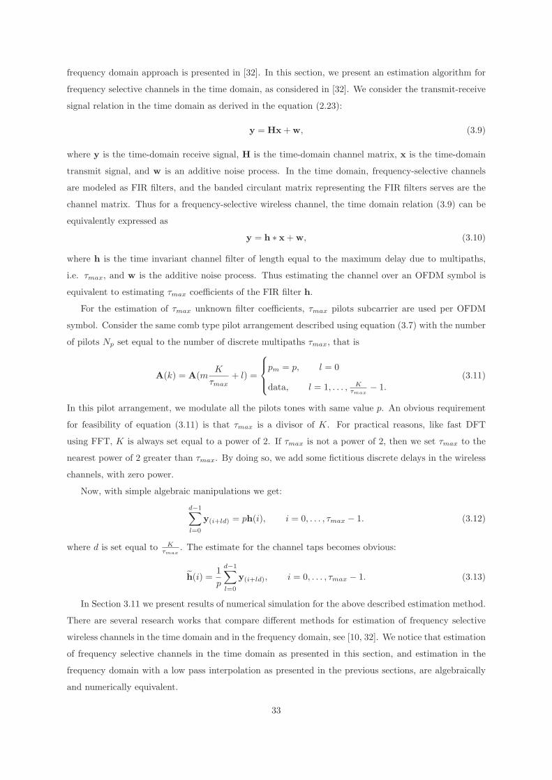
frequency domain approach is presented in [32]. In this section, we present an estimation algorithm for

frequency selective channels in the time domain, as considered in [32]. We consider the transmit-receive

signal relation in the time domain as derived in the equation (2.23):

y = Hx+w, (3.9)

where y is the time-domain receive signal, H is the time-domain channel matrix, x is the time-domain

transmit signal, and w is an additive noise process. In the time domain, frequency-selective channels

are modeled as FIR filters, and the banded circulant matrix representing the FIR filters serves are the

channel matrix. Thus for a frequency-selective wireless channel, the time domain relation (3.9) can be

equivalently expressed as

y = h ∗ x+w, (3.10)

where h is the time invariant channel filter of length equal to the maximum delay due to multipaths,

i.e. τmax, and w is the additive noise process. Thus estimating the channel over an OFDM symbol is

equivalent to estimating τmax coefficients of the FIR filter h.

For the estimation of τmax unknown filter coefficients, τmax pilots subcarrier are used per OFDM

symbol. Consider the same comb type pilot arrangement described using equation (3.7) with the number

of pilots Np set equal to the number of discrete multipaths τmax, that is

A(k) = A(mK

τmax

+ l) =

pm = p, l = 0

data, l = 1, . . . , Kτmax

− 1.

(3.11)

In this pilot arrangement, we modulate all the pilots tones with same value p. An obvious requirement

for feasibility of equation (3.11) is that τmax is a divisor of K. For practical reasons, like fast DFT

using FFT, K is always set equal to a power of 2. If τmax is not a power of 2, then we set τmax to the

nearest power of 2 greater than τmax. By doing so, we add some fictitious discrete delays in the wireless

channels, with zero power.

Now, with simple algebraic manipulations we get:

d−1∑

l=0

y(i+ld) = ph(i), i = 0, . . . , τmax − 1. (3.12)

where d is set equal to Kτmax

. The estimate for the channel taps becomes obvious:

h(i) =1

p

d−1∑

l=0

y(i+ld), i = 0, . . . , τmax − 1. (3.13)

In Section 3.11 we present results of numerical simulation for the above described estimation method.

There are several research works that compare different methods for estimation of frequency selective

wireless channels in the time domain and in the frequency domain, see [10, 32]. We notice that estimation

of frequency selective channels in the time domain as presented in this section, and estimation in the

frequency domain with a low pass interpolation as presented in the previous sections, are algebraically

and numerically equivalent.

33

3.7 Doubly-Selective Channels

In the last two decades, there has been a steady increase in the number of applications utilizing rapidly

varying wireless communication channels. Such channels occur due to user mobility in the systems

like DVB-T and WiMAX, which have been originally designed for fixed receivers. Such channels are

commonly known as doubly-selective channels, because such channels are frequency-selective due to the

multipath effect and time-selective due to the Doppler effect. Unlike frequency-selective channels, the

channel matrix corresponding to the doubly-selective channels are not diagonal in the frequency domain.

The off-diagonal entries in the frequency domain channel matrix lead to intercarrier interference (ICI) in

multicarrier communication systems like OFDM. Wireless channel estimation and equalization methods

for communication systems encountering doubly-selective channels are need to mitigate the effects of

ICI.

The basis expansion model (BEM) is commonly used for modeling doubly-selective channels. With a

BEM, the channel taps, i.e. the discrete time-varying filter coefficients of the channel, h, are expressed as

linear combinations of certain basis functions. In this dissertation, we use the BEM for wireless channel

estimation, as well as equalization. In the next section, we describe the BEM in more detail.

Another way of modeling doubly selective channels is by assuming a banded structure of the channel

matrix in the frequency domain. Consider the frequency domain channel matrix given by equation (3.2),

i.e.

Y = Fy = FHF∗Fx+ Fw. (3.14)

Unlike frequency-selective channels, the frequency domain channel matrix H = FHF∗ of the doubly-

selective channel is not diagonal anymore. Instead, the frequency domain channel matrix H is approxi-

mated as a banded matrix. Alternatively, this approach can be interpreted as approximating ICI only of

a few neighboring subcarriers. Such a model for doubly-selective wireless channels and has been exploited

for equalizer design, see [47, 37]. ICI-shaping, which concentrates the ICI power within a small band of

the channel matrix, is described in [47, 41].

3.8 Basis Expansion Model

The basis expansion model (BEM) is a commonly used method for modeling time-varying doubly-selective

channels. With a BEM, the time-varying channel taps, i.e. the time-varying filter coefficients of the

doubly-selective channels, hl, are expressed as linear combinations of certain basis functions. Thus the

l-th discrete channel tap hl is modeled as:

hl =M−1∑

m=0

blmBm, l = 0, . . . , L− 1, (3.15)

where {Bm} is the set of M basis functions used to express the channel taps, and L is the maximum

discrete path delay, see [49, 15, 54, 45, 46, 42, 21]. In this context, channel estimation amounts to an

approximate computation of coefficients for the basis functions, i.e. blm. Several methods for wireless

34

(a) doubly-selective channel tap

(b) Fourier basis

(c) polynomial basis

Figure 3.5: Real part of a doubly-selective channel tap, along with real part of Fourier basis and Legendre

Polynomial basis

35

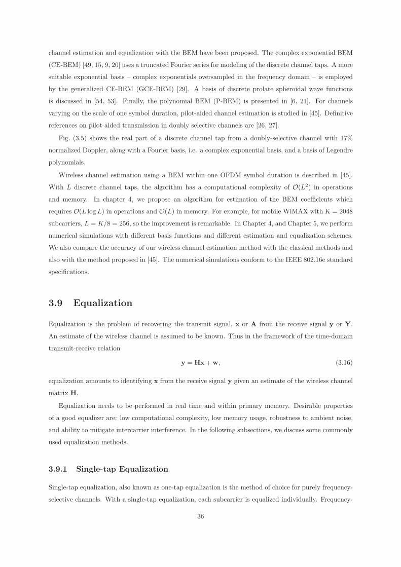
channel estimation and equalization with the BEM have been proposed. The complex exponential BEM

(CE-BEM) [49, 15, 9, 20] uses a truncated Fourier series for modeling of the discrete channel taps. A more

suitable exponential basis – complex exponentials oversampled in the frequency domain – is employed

by the generalized CE-BEM (GCE-BEM) [29]. A basis of discrete prolate spheroidal wave functions

is discussed in [54, 53]. Finally, the polynomial BEM (P-BEM) is presented in [6, 21]. For channels

varying on the scale of one symbol duration, pilot-aided channel estimation is studied in [45]. Definitive

references on pilot-aided transmission in doubly selective channels are [26, 27].

Fig. (3.5) shows the real part of a discrete channel tap from a doubly-selective channel with 17%

normalized Doppler, along with a Fourier basis, i.e. a complex exponential basis, and a basis of Legendre

polynomials.

Wireless channel estimation using a BEM within one OFDM symbol duration is described in [45].

With L discrete channel taps, the algorithm has a computational complexity of O(L2) in operations

and memory. In chapter 4, we propose an algorithm for estimation of the BEM coefficients which

requires O(L logL) in operations and O(L) in memory. For example, for mobile WiMAX with K = 2048

subcarriers, L = K/8 = 256, so the improvement is remarkable. In Chapter 4, and Chapter 5, we perform

numerical simulations with different basis functions and different estimation and equalization schemes.

We also compare the accuracy of our wireless channel estimation method with the classical methods and

also with the method proposed in [45]. The numerical simulations conform to the IEEE 802.16e standard

specifications.

3.9 Equalization

Equalization is the problem of recovering the transmit signal, x or A from the receive signal y or Y.

An estimate of the wireless channel is assumed to be known. Thus in the framework of the time-domain

transmit-receive relation

y = Hx+w, (3.16)

equalization amounts to identifying x from the receive signal y given an estimate of the wireless channel

matrix H.

Equalization needs to be performed in real time and within primary memory. Desirable properties

of a good equalizer are: low computational complexity, low memory usage, robustness to ambient noise,

and ability to mitigate intercarrier interference. In the following subsections, we discuss some commonly

used equalization methods.

3.9.1 Single-tap Equalization

Single-tap equalization, also known as one-tap equalization is the method of choice for purely frequency-

selective channels. With a single-tap equalization, each subcarrier is equalized individually. Frequency-

36

selective channel matrix is diagonal in the frequency domain, see equation (3.3), which is

Y = DA+W. (3.17)

The diagonal entries of the frequency-domain channel matrix D are efficiently estimated by using pilot

information, see Section 3.5 for details. Thus the equalized frequency-domain receive signal is given by

A(k) =Y(k)

D(k, k), k = 1, . . . ,K, (3.18)

where D is the estimated channel and A is the equalized frequency-domain transmit signal. In the

absence of any further statistical information about the data, single-tap equalization method is optimal

in the least squares sense. If an approximate signal to noise ratio (SNR) of the additive noise W is

known, the equalized signal can be improved in the following manner:

A(k) =Y(k)conj(D(k, k))

|D(k, k)|+ 1SNR

. k = 1, . . . ,K, (3.19)

The above equalization method using the SNR is a shrinkage estimator, where a priori knowledge of the

signal to noise ratio is used to bound the power of the equalized signal.

3.9.2 Doubly Selective Channel Equalization

Basis expansion models (BEM) are used for estimating doubly-selective channels. With a BEM, wireless

channel estimation amounts to finding the coefficients of the basis functions used to model the wire-

less channel taps. Usually, the channel matrix is reconstructed from estimated BEM coefficients and

subsequently used in equalization.

With severe ICI, the conventional single-tap equalization in the frequency domain is unreliable, see

[36, 30, 38]. Several other approaches have been proposed to combat ICI in transmissions over rapidly

varying doubly-selective channels. For example, [8] presents minimum mean-square error (MMSE) and

successive interference cancellation equalizers, which use all subcarriers simultaneously. However, the

methods are computationally expensive. Alternatively, using only a few subcarriers in equalization

amounts to approximating the frequency-domain channel matrix by a banded matrix, and has been

exploited for equalizer design, see [47, 37]. ICI-shaping, which concentrates the ICI power within a small

band of the channel matrix, is described in [47, 41]. A banded matrix approximation of doubly-selective

wireless channels mitigates ICI partially, because intercarrier interference from carriers outside the band

is not considered. A low-complexity time-domain equalizer based on the LSQR algorithm is introduced

in [22]. This method produces accurate results, but requires O(K2) operations and O(K2) in memory.

In Chapter 5, we present a novel equalization algorithm, that uses the BEM coefficients directly, without

ever creating the channel matrix.

37

Order of DFT (K) 256

Cyclic Prefix 32

Symbol duration 102.9 µs

Carrier Frequency 5.8 GHz

Bandwidth 5.16 MHz

Alphabet 4QAM

Binary coding rate 1/2 with bit interleaving

Table 3.1: Transmission parameters for mobile WiMAX (IEEE 802.16e)

3.10 Simulation Setup

In this section we describe our simulation setup for testing of wireless channel estimation and equalization

algorithms. In the next section we report the performance of wireless channel estimation and equalization

algorithms designed for frequency selective channels. We also report results about performance of those

algorithms in doubly-selective wireless channels.

Our simulation parameters conforms mobile WiMAX (IEEE 802.16e), which is an important ap-

plication of OFDM. The same setup, with different parameters can be used for other applications

like digital video broadcasting (terrestrial) DVB-T, wireless access in vehicular environment (WAVE).

We simulate a coded OFDM system with K = 256 subcarriers, utilizing B = 2.8MHz of bandwidth

at a carrier frequency of fc = 5.8GHz. We use a cyclic prefix of length Lcp = 32 in order to

avoid ISI. Consequently, the sampling period is Ts = 1/B = 0.357µs, and the symbol duration is

(K + Lcp)Ts = (256 + 32)× 0.357µs = 102.9µs. The information bits are encoded using a convolutional

code of rate 1/2, passed through an interleaver, and mapped to 4-QAM symbols. See Table 3.1 for a

quick reference.

A Rayleigh Fading WSSUS channel with Jakes Doppler spectrum is simulated for testing of the

wireless channel estimation and equalization algorithms. We use them MATLAB communication toolbox

(V 3.4) for simulation of the wireless channel. Maximum Doppler shifts are calculated using the formula

νmax =v

cfc, (3.20)

where fc is the carrier frequency, v is the relative velocity between receiver and transmitter, c is the

velocity of electromagnetic wave. See Table 3.2 for a quick reference.

3.11 Results of Simulations

In this section we report computer simulation results of wireless channel estimation algorithms designed

for frequency selective wireless channels. We use single tap equalization with the estimated channel.

Wireless channel estimation is done in the frequency domain as well as in the time domain. Since time-

domain channel estimation coincides with frequency domain channel estimation combined with low pass

38

Maximum vehicular speed 25 km/h

Maximum path delay 11.4 µs

Maximum Doppler shift 0.13 kHz

Average path gain -2 dB

Fading Rayleigh

Doppler spectrum Jakes

Table 3.2: Parameters for wireless channel simulation

0 5 10 15 20 25 30 35 4010

−8

10−6

10−4

10−2

Eb/N0 [dB]

BE

R

low passcubic splinelinear

Figure 3.6: BER vs. Eb/N0 at zero receiver velocity

interpolation, we do not plot the curve for time domain channel estimation. Frequency domain channel

estimation is done by estimating the frequency attenuation at the pilot carriers, and then interpolating

the frequency attenuation over the data carriers. We use linear interpolation, cubic spline interpolation,

and low pass interpolation. We report the bit error rate (BER) after decoding with the BCJR algorithm.

Figure 3.6 shows the BER as a function of energy per bit to noise spectral density (Eb/N0). We

notice that estimation with low pass interpolation is the best among the three interpolation schemes.

All the three curves finally saturate at a high Eb/N0, i.e. at very small ambient noise. We note that

linear interpolation has the smallest computational complexity, i.e. O(K), where K is the number

of OFDM subcarriers. Complexity of interpolation with cubic splines is a constant factor more that

linear interpolation, but still O(K) operations. The low pass interpolation is done using FFT and has a

computational complexity of O(K logK).

Figure 3.7 shows the BER as a function of energy per bit to noise spectral density (Eb/N0), but

the simulated wireless channel is generated for a vehicular speed to 20 km/h, which is equivalent to

a Doppler shift of 0.13 kHz. The described channel estimation algorithms assume that the frequency

domain channel matrix is diagonal. Therefore, the intercarrier interference caused by the Doppler effect

39

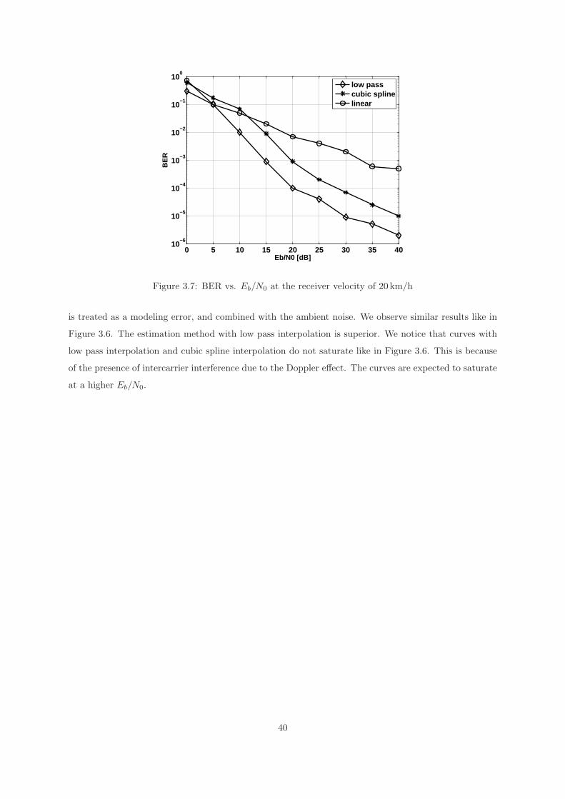
0 5 10 15 20 25 30 35 4010

−6

10−5

10−4

10−3

10−2

10−1

100

Eb/N0 [dB]

BE

R

low passcubic splinelinear

Figure 3.7: BER vs. Eb/N0 at the receiver velocity of 20 km/h

is treated as a modeling error, and combined with the ambient noise. We observe similar results like in

Figure 3.6. The estimation method with low pass interpolation is superior. We notice that curves with

low pass interpolation and cubic spline interpolation do not saturate like in Figure 3.6. This is because

of the presence of intercarrier interference due to the Doppler effect. The curves are expected to saturate

at a higher Eb/N0.

40

Chapter 4

Estimation of rapidly varying

channels in OFDM systems using a

BEM with Legendre polynomials

4.1 Introduction

4.1.1 Overview

In this chapter we propose a novel pilot-aided scheme for estimation of rapidly varying wireless channels

in OFDM systems. Our approach is aimed at channels varying on the scale of a single OFDM symbol

duration, and uses a simple arrangement of pilots in uniformly spaced blocks within each OFDM symbol.

We develop a fast and accurate algorithm for computation of the Fourier coefficients of the channel taps

within an individual OFDM symbol duration. Since the representation of the channel taps as a truncated

Fourier series (Basis Expansion Model with complex exponentials, CE-BEM) is inaccurate due to the

Gibbs phenomenon, we reconstruct the taps as a truncated Legendre series, in the framework of the Basis

Expansion Model (BEM) with the Legendre polynomials. In this way, we use a priori information that

the channel taps are analytic but not necessarily periodic, and obtain realistic approximate channel taps.

For systems with L discrete channel taps, our method uses O(L logL) operations and O(L) memory

per OFDM symbol, which is best possible up the order of magnitude. Previously published methods

[45] requires O(L2) both in operations and in memory. We use Legendre polynomials because of its

several desirable properties, but any other basis can be used in the proposed framework, with the same

complexity. We derive explicit formulas for the Legendre coefficients in terms of the Fourier coefficients.

Numerical simulations illustrate performance gains achieved by our estimator at sufficiently high Doppler

frequencies. Our approach does not assume any prior statistical information.

1Part of this chapter is submitted for a journal publication

41

4.1.2 Motivation and Previous Work

Orthogonal frequency-division multiplexing (OFDM) is a popular multicarrier modulation technique

with several desirable features, e.g. robustness against multipath propagation and high spectral efficiency.

OFDM is increasingly used in high-mobility wireless communication systems, e.g. mobile WiMAX (IEEE

802.16e), WAVE (IEEE 802.11p), and 3GPP’s UMTS Long-Term Evolution (LTE). Usually OFDM

systems are designed so that no channel variations occur within an individual OFDM symbol duration.

Recently, however, there has been an increasing interest in rapidly varying channels, where the channel

coherence time is less than the OFDM symbol duration. In such situations, strong intercarrier interference

(ICI) becomes a major source of transmission impairment (in addition to fading and noise). ICI is caused

by user mobility, moving reflectors, or substantial carrier frequency offsets. For example, severe ICI occurs

during a WiMAX transmission in the proximity of a highway.

In the case of frequency-selective channels in OFDM systems, estimation in the frequency-domain is

unmatched in simplicity and accuracy, see Sections 3.3 and 3.5. On the other hand, in doubly-selective

channels, see Section 3.7, both time- and frequency-domain approaches have been used. The Basis

Expansion Model (BEM) approximates the channel taps by combinations of prescribed basis functions,

[54, 45, 46, 42], see Section 3.8. In this context, channel estimation amounts to approximate computation

of the basis coefficients. The BEM with complex exponential (CE-BEM) [9, 20] uses a truncated Fourier

series, and is remarkable because the resulting frequency-domain channel matrix is banded. However,

this method has a limited accuracy due to a large modeling error. Specifically, [53, 54] observe that the

reconstruction with a truncated Fourier series introduces significant distortions at the ends of the data

block. The errors are due to the Gibbs phenomenon, and manifest themselves as a spectral leakage,

especially in the presence of significant Doppler spreads. A more suitable exponential basis is provided

by the Generalized CE-BEM (GCE-BEM) [29], which employs complex exponentials oversampled in the

frequency domain. A basis of discrete prolate spheroidal wave functions is discussed in [53, 54]. Finally,

the polynomial BEM (P-BEM) is presented in [6]. For channels varying at the scale of one OFDM

symbol duration, pilot-aided channel estimation is studied in [45].

Definitive references on pilot-aided transmission in doubly-selective channels are [26, 27].

4.1.3 Contributions

The main contributions of this work can be summarized as follows.

• We propose a pilot-aided method for channel estimation in OFDM systems, which explicitly sepa-

rates the computation of the Fourier coefficients of the channel taps, and a subsequent computation

of BEM coefficients of the channel taps.

• We formulate a numerically stable algorithm for the approximate computation of the Fourier coeffi-

cients of the channel taps from the receive signal, assuming a uniform, FDKD-type pilot placement.

The proposed method requires O(L logL) operations, where L is the number of discrete channel

42

taps, and uses only subsampling of the frequency-domain receive signal and linear operations with

condition number equal to 1.

• We propose a method for reconstruction of the channel taps using a truncated Legendre series in

order to mitigate the Gibbs phenomenon. We derive explicit formulas for the Legendre coefficients

in terms of estimated Fourier coefficients.

Extensive computer simulations show that at high mobile velocities, our scheme is superior to the

conventional single tap least squares (LS) estimation [10], estimation with a Basis Expansion Model using

complex exponentials (CE-BEM) [27], and LS estimation scheme proposed in [45]. Our transmission

simulation setup conforms to the WiMAX standards (IEEE 802.16e). For computer simulations, we

filter transmit signals through rapidly varying channels, typically simulated for a relative velocity of 300

km/h, and energy per bit to noise spectral density (Eb/N0) of 20 dB.

This chapter is further organized in the following way. In Section 4.2, we discuss theoretical foun-

dations of the proposed estimation algorithm. In Section 4.3, we introduce the system model, and then

the proposed channel estimator in Section 4.4. We present simulation results in Section 4.5, and chapter

conclusions in Section 4.6.

4.2 Theoretical Foundations of the Estimation Algorithm

4.2.1 Overview

We develop a systematic framework for channel estimation in OFDM systems with significant channel

variations within one OFDM symbol duration. We divide this task into two separate steps,

• pilot-aided estimation of the Fourier coefficients of the channel taps.

• estimating BEM coefficients from the estimated Fourier coefficients.

4.2.2 Fourier Coefficients of Channel Taps

We use pilot symbol assisted modulation (PSAM), with uniformly distributed blocks of pilot sub-carriers,

each block having the frequency-domain Kronecker delta (FDKD) pilot arrangement [26, 27]. Pilots are

inserted in every OFDM symbol in order to capture rapid variations of path gains. The first few Fourier

coefficients of the channel taps are computed for each individual OFDM symbol. In Subsection 4.4.3, we

derive an efficient, numerically stable method for estimation of the Fourier coefficients of the channel taps

from the time-domain receive signal. A straightforward reconstruction of the channel taps as truncated

Fourier series from the estimated Fourier coefficients is inaccurate. This problem is well known, and

is commonly referred to as the Gibbs phenomenon. In the context of wireless channels, the Gibbs

phenomena is highlighted in [53]. However, it turns out that the information content of the Fourier

coefficients can be used more effectively than in the straightforward approach, as we explain in the next

subsection.

43

4.2.3 BEM with Legendre Polynomials

The second stage is to estimate the BEM coefficients of the channel taps from their Fourier coefficients

in a way which remedies the Gibbs phenomenon. Several accurate algorithms have been proposed for

this task, see [17, 44, 12]. We have chosen the reconstruction with the Legendre polynomials adapted to

individual OFDM symbols (see Subsection 4.4.4 for details), which amounts to a BEM with the Legendre

polynomials. In next few paragraphs we discuss motivation behind considering Legendre polynomials

for BEM.

We make an a priori assumption that the channel taps are analytic, but not necessarily periodic.

Most of such functions can be represented well by truncated Legendre series [7].

The number of the Fourier coefficients of the wireless channel taps that can be estimated is limited

by the number of pilot subcarriers. By increasing the number of pilot subcarriers, we can compute more

Fourier coefficients, see Section 4.4.3, but doing so reduces the spectral efficiency, and consequently the

final throughput of the whole communication setup. Typically, 2, 3, 4, or 5 Fourier coefficients of each of

the channel taps are computed from the pilot information. The Gibbs phenomenon can be mitigated by

projecting the truncated Fourier series on algebraic polynomials, see [17]. A conventional way to describe

such projections uses the basis of the Gegenbauer polynomials, specifically the Legendre polynomials.

The Legendre polynomials are analytic solutions of the Legendre differential equation:

(1− x2)y′′ − 2xy′ + n(n+ 1)y = 0. (4.1)

In [53, 54], the authors argue that the channel taps are bandlimited functions, with the bandlimit of

the channel tap proportional to the Doppler shift. For modeling of the wireless channel taps [54, 45] use

discrete prolate spheroidal sequences, i.e. the Slepian sequences, for BEM, which give rise to bandlimited

wireless channel taps. Assuming the channel taps to be analytic, one can also consider the prolate

spheroidal wave functions [43], the continuous counter part of discrete prolate spheroidal sequences. The

prolate spheroidal wave functions are analytic solutions of the differential equation [43]:

(1− x2)y′′ − 2xy′ + (λctb − c2tbx2)y = 0, (4.2)

where ctb is the time-bandwidth product, i.e. the product of the fixed length of the time interval, and

the frequency bandwidth in which the most of the energy of the function is concentrated.

We estimate the wireless channel taps within one OFDM symbol duration, which is a very small

period to time. For example in mobile-WiMAX the useful symbol duration is T = 91.4µs, carrier

frequency of fc = 5.8GHz, and a relative velocity of v = 200Km/h, the time-bandwidth product of the

channel taps is given by:

ctb = Tνmax = Tv

cfc = 0.09. (4.3)

Here c is the velocity of light. Thus it is reasonable for us to consider ctb to be very very small. If we

now set ctb equal to zero and λctb = n(n + 1) in equation (4.2), it will be identical to equation (4.1).

Analytic solutions of this differential equation are known as Legendre polynomials. See Figure 4.1 for a

graphical view demonstrating the motivation behind the choice of Legendre polynomials for BEM.

44

Channel taps are analytic andnot necessarily

periodic

Channel tapsare optimallybandlimited

Resolve Gibbsphenomenon

Fouriercoefficients

with few

polynomials

Gegenbauer

wave Spheroidal

Prolate

functions

Legendre

polynomials

Figure 4.1: Motivation behind choice of Legendre polynomials

A truncated Fourier series is converted into a truncated Legendre series by orthogonal projection on

the space of algebraic polynomials of a fixed degree. No truncated Fourier series is ever formed. Instead,

the Legendre coefficients are computed from the estimated Fourier coefficients by applying a matrix,

whose entries have explicit expressions in terms of the spherical Bessel functions of the first kind [14],

see Subsection 4.4.4. Specifically, the entries are the Legendre coefficients of complex exponentials.

Although the Legendre coefficients are computed from the estimated Fourier coefficients, a truncated

Legendre series is in fact more accurate than a truncated Fourier series with a similar number of terms.

The quality of the reconstruction with the truncated Legendre series is illustrated in Figure 4.2, where the

real part of a typical channel tap is plotted along with its approximation by a truncated Fourier series and

a truncated Legendre series. In Figure 4.2, we use a two-term Legendre series, which amounts to a linear

function, and a three-term Fourier series, see Section 4.4 for details. We emphasize, that our proposed

algorithm does not create a truncated Fourier series itself, but rather computes estimated Legendre

coefficients from estimated Fourier coefficients. Our numerical simulations confirm that estimation with

a truncated Legendre series is dramatically more accurate than the reconstruction with a truncated

Fourier series.

The Fourier coefficients can be computed using systematically placed pilot carriers, see Subsec-

tions 4.4.1 and 4.4.3. The crucial point is that equation (4.15) used for the estimation of the Fourier

coefficients does not involve unknown data symbols, so the Fourier coefficients depend only on the known

pilot values.

45

0 20 40 60 80 96.840

0.02

0.04

0.06

0.08

0.1

0.12

0.14

time [ µs]

ch

an

ne

l ta

p p

ath

ga

in (

rea

l p

art

)

FourierLegendreexact

Figure 4.2: A typical channel tap (real part) across one OFDM symbol, the normalized Doppler equals

20%.

4.3 System Model

4.3.1 Transmitter-Receiver Model

We consider an equivalent baseband representation of a single-antenna OFDM system withK subcarriers.

We assume a sampling period of Ts = 1/B, where B denotes the transmit bandwidth. A cyclic prefix

of length Lcp is used in every OFDM symbol. We choose Lcp so large that LcpTs exceeds the channel’s

maximum delay, in order to avoid inter symbol interference (ISI). Consequently, throughout this paper,

we deal with one OFDM symbol at a time.

Each subcarrier is used to transmit a symbol A[k] (k = 0, . . . ,K − 1) from a finite symbol constella-

tion. A subset of these symbols serves as pilots for channel estimation (cf. Section 4.4.3). The OFDM

modulator uses the inverse discrete Fourier transform (IDFT) to map the frequency-domain transmit

symbols A[k] to the time-domain transmit signal x[n]

x[n] =1√K

K−1∑

k=0

A[k] e2πnkK , (4.4)

n = −Lcp, . . . ,K−1.

After discarding the cyclic prefix, the receive signal satisfies

y[n] =

L−1∑

l=0

hl[n]x[n− l] + w[n], n = 0, . . . ,K − 1. (4.5)

Here, w[n] denotes circularly complex additive noise of variance N0, hl[n] is the complex channel tap

associated with delay l, and L is the channel length (maximum discrete-time delay). Consequently, the

46

channel’s maximum delay equals (L−1)Ts. For simplicity, we make the worst-case assumption L = Lcp.

The OFDM demodulator performs a DFT to obtain the frequency-domain receive signal

Y [k]=1√K

K−1∑

n=0

y[n] e−2π nkK =

L−1∑

l=0

(Hl ∗Xl)[k] +W [k], (4.6)

where ∗ denotes the cyclic convolution, and k = 0, . . . ,K − 1. In this expression, Y [k], Hl[k], Xl[k], and

W [k] denote the DFT of y[n], hl[n], x[n− l], and w[n], respectively. Specifically,

Hl[k] =1√K

K−1∑

n=0

hl[n] e−2π nk

K (4.7)

are the Fourier coefficients of the individual channel taps, and

Xl[k] = e−2π lkK A[k] . (4.8)

4.3.2 BEM with Legendre Polynomials

As discussed above, we use basis of the Legendre polynomials because of its certain desirable properties,

any other basis can be treated in a similar way within the developed framework. Each channel tap

hl[n] is modeled as a linear combination of the first M Legendre polynomials rescaled to a single OFDM

symbol duration (without the cyclic prefix)

hl[n] =

M−1∑

m=0

blm pm[n] , l = 0, . . . , L−1, (4.9)

where blm is the mth Legendre coefficient of the lth channel tap, and M is the BEM model order.

Furthermore,

pm[t] = Pm

(2t

KTs

− 1

), t ∈ [0,KTs], (4.10)

where Pm is the Legendre polynomial of degree m, as defined in [18], equation (8.910). For any other

basis, a similar rescaling need to be done to adopt them within one OFDM symbol duration.

4.4 Proposed Channel Estimator

4.4.1 Analysis of Intercarrier Interactions

In our system model, channel estimation amounts to computing the LM Legendre coefficients {blm}from the receive signal Y [k] (y[n]) and the pilot symbols. We first estimate the Fourier coefficients of

the channel taps (cf. (4.7)), and then we compute approximate Legendre coefficients from the Fourier

coefficients, as discussed in Section 4.4.4.

For a fixed positive integer D, we approximate the channel taps with their D-term Fourier series

hl[n] ≈D+∑

d=D−

Hl[d] e2π dn

K , (4.11)

47

where D− = −⌊(D−1)/2⌋ and D+ = ⌊D/2⌋ (⌊·⌋ denotes the floor operation). Clearly, D− 6 0 6 D+,

and D+−D− = D−1. The representation of the channel taps described by equation (4.11) is commonly

known as the Basis Expansion Model with complex exponentials (CE-BEM) [9, 20]. We use this model

only for computation of the Fourier coefficients of the channel taps, but not for reconstruction of the

taps themselves. Combining (5.2), (4.6), (4.8) and (4.11), we obtain

Y [k] =

L−1∑

l=0

D+∑

d=D−

Hl[d]Xl[k − d] + W [k]

=

L−1∑

l=0

D+∑

d=D−

Hl[d] e−2π

l(k−d)K A[k−d] + W [k],

=

D+∑

d=D−

A[k−d]

L−1∑

l=0

Hl[d] e−2π

l(k−d)K + W [k], (4.12)

where k = 0, . . . ,K − 1, and W [k] denotes the additive noise W [k] combined with the approximation

error resulting from (4.11). From the above equation, we notice that the value Y [k] depends only on

the 2D − 1 transmit symbols A[k −D+],. . . , A[k −D−] at the neighboring subcarriers.

4.4.2 Pilot Arrangement

We assume that I = KL

is an integer, which can always be achieved by an appropriate choice of L. Since

K is always a power of 2 for practical reasons, the best way to make I an integer is to set L to the

nearest power of 2, thereby adding some fictitious channel taps. This assumption is crucial for numerical

stability of the algorithm described in Subsection 4.4.3, and also helps in reducing the computational

complexity of the algorithm. Within each OFDM symbol, we distribute pilots in the frequency domain

in L blocks of size 2D − 1 each, uniformly spaced every I subcarriers. Of course, this is only possible if

2D − 1 6 I. Denoting the location of the first pilot subcarrier by k0, 0 6 k0 6 I − (2D − 1), the pilot

locations have the form

k0 + q + iI, (4.13)

where q = 0, . . . , 2D−2, and i = 0, . . . , L−1. An example of such an arrangement is shown in Figure 4.3.

Within each block, all the pilot values are zero, except for the central pilot, which is set to a value a0

common to all blocks. Thus only the L symbols A[k0 + D − 1 + iI], i = 0, . . . , L − 1, carry non-zero

pilots.

4.4.3 Estimation of Fourier Coefficients

We create D length-L subsequences of the frequency-domain receive signal Y [k] by uniform subsampling

as follows

Yd[i] = Y [k0 +D+ + d+ iI], (4.14)

48

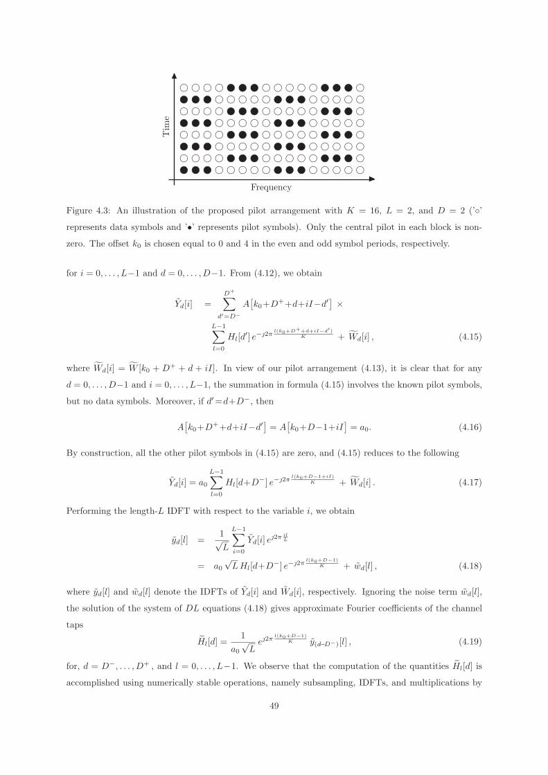
g

g

g

g

g

g

g

g

g

g

g

g

g

g

g

g

g

g

g

g

g

g

g

g

g

g

g

g

g

g

g

g

g

g

g

g

g

g

g

g

g

g

g

g

g

g

g

g

g

g

g

g

g

g

g

g

g

g

g

g

g

g

g

g

g

g

g

g

g

g

g

g

g

g

g

g

g

g

g

g

g

g

g

g

g

g

g

g

g

g

g

g

g

g

g

g

g

g

g

g

g

g

g

g

g

g

g

g

g

g

g

g

g

g

g

g

g

g

g

g

g

g

g

g

g

g

g

g

w

w

w

w

w

w

w

w

w

w

w

w

w

w

w

w

w

w

w

w

w

w

w

w

w

w

w

w

w

w

w

w

w

w

w

w

w

w

w

w

w

w

w

w

w

w

w

w6

-

N

◮

Tim

e

Frequency

Figure 4.3: An illustration of the proposed pilot arrangement with K = 16, L = 2, and D = 2 (’◦’represents data symbols and ’•’ represents pilot symbols). Only the central pilot in each block is non-

zero. The offset k0 is chosen equal to 0 and 4 in the even and odd symbol periods, respectively.

for i = 0, . . . , L−1 and d = 0, . . . , D−1. From (4.12), we obtain

Yd[i] =

D+∑

d′=D−

A[k0+D++d+iI−d′

]×

L−1∑

l=0

Hl[d′] e−2π

l(k0+D++d+iI−d′)K + Wd[i] , (4.15)

where Wd[i] = W [k0 + D+ + d + iI]. In view of our pilot arrangement (4.13), it is clear that for any

d = 0, . . . , D−1 and i = 0, . . . , L−1, the summation in formula (4.15) involves the known pilot symbols,

but no data symbols. Moreover, if d′=d+D−, then

A[k0+D++d+iI−d′

]= A

[k0+D−1+iI

]= a0. (4.16)

By construction, all the other pilot symbols in (4.15) are zero, and (4.15) reduces to the following

Yd[i] = a0

L−1∑

l=0

Hl[d+D−] e−2πl(k0+D−1+iI)

K + Wd[i] . (4.17)

Performing the length-L IDFT with respect to the variable i, we obtain

yd[l] =1√L

L−1∑

i=0

Yd[i] e2π il

L

= a0√LHl[d+D−] e−2π

l(k0+D−1)K + wd[l] , (4.18)

where yd[l] and wd[l] denote the IDFTs of Yd[i] and Wd[i], respectively. Ignoring the noise term wd[l],

the solution of the system of DL equations (4.18) gives approximate Fourier coefficients of the channel

taps

Hl[d] =1

a0√Le2π

l(k0+D−1)K y(d−D−)[l] , (4.19)

for, d = D−, . . . , D+ , and l = 0, . . . , L−1. We observe that the computation of the quantities Hl[d] is

accomplished using numerically stable operations, namely subsampling, IDFTs, and multiplications by

49

scalars of equal magnitudes. On the other hand, previous approaches to the computation of the Fourier

(CE-BEM) coefficients from the receive signal over one OFDM symbol require O(K2) operations, and

do not control the condition numbers, see subsection IV-B in [45].

Reconstruction of the channel taps as truncated Fourier series using equation (4.11) and the estimated

Fourier coefficients (4.19) is inaccurate because of the Gibbs phenomenon, see Fig 4.2. In the next

subsection, we demonstrate a simple method for the mitigation of the Gibbs phenomenon using a priori

information.

4.4.4 Estimation of Legendre Coefficients

As discussed above, the basis of Legendre polynomials are used because of its certain desirable properties,

and we demonstrate the procedure of computation of Legendre coefficients of the channel taps from

estimated Fourier coefficients. But the same framework can be used with to find expansion coefficients

of channel taps with respect to arbitrary basis functions as well. We regard the channel taps as analytic

functions of time, and represent them by means of a rapidly converging expansion known as the Legendre

series [7]. It turns out, that one of the simplest methods to reduce the Gibbs phenomenon is to convert

a truncated Fourier series into a truncated Legendre series by orthogonal projection. We describe how

this is accomplished by a linear mapping transforming the Fourier coefficients into approximate Legendre

coefficients, without ever creating the truncated Fourier series (4.11) explicitly.

In order to derive this linear mapping, let us project the truncated Fourier expansion (see equa-

tion (4.11)) onto the rescaled Legendre polynomials pm (see equation (4.10)), which form an orthogonal

basis on the interval [0,KTs]. The mth Legendre coefficient of the exponential function e2πd

KTst equals

∫KTs

0e2π

dKTs

tpm(t)dt∫KTs

0p2m(t)dt

=(−1)d

∫ 1

−1eπdxPm(x)dx

∫ 1

−1P 2m(x)dx

= m(2m+ 1) (−1)d jm(πd), (4.20)

where jm is the spherical Bessel function of the first kind and order m (see [1], formula 10.1.1, and [18],

formula 7.243). Combining this equation with (4.9) and (4.11), we obtain

blm = m(2m+1)

D+∑

d=D−

(−1)d jm(πd) Hl[d] , (4.21)

where blm denotes the estimate of blm. The linear mapping (4.21) amounts to applying the M × D

matrix J with entries

Jmd = (m−1)(2m−1) (−1)d jm−1

(π(d−D+)

)(4.22)

to the length-D vector (Hl[D−], . . . , Hl[D

+])T of the estimated Fourier coefficients, resulting in the

length-M vector (bl0, . . . , bl(M−1))T of the Legendre coefficients.

For D = 1, 2, 3 and M = 1, 2, 3, we have verified experimentally that matrix J has condition

number less than or equal to 2.15 (equality holds for D = 3, and M = 3). Since the approximate Fourier

coefficients themselves are computed with the DFTs, the overall estimation of the Legendre coefficients

50

step description flops example

1 L-point IDFTs of Yk[i] DL logL 480

2 computation of Fourier coeff. DL 96

3 computation of Legendre coeff. MDL 192

Table 4.1: Complex flop count for the proposed algorithm per OFDM symbol obtained for K = 256,

L = 32, D = 3, and M = 2 (as used in the simulations).

from the receive signal is numerically stable. Finally, the channel taps are reconstructed as truncated

Legendre series using the coefficients blm as in equation (4.9)

hl[n] =

M−1∑

m=0

blm pm[n] , l = 0, . . . , L−1. (4.23)

Fig. 4.2 demonstrates effectiveness of the reconstruction of the channel taps as truncated Legendre series.

Although the Legendre coefficients are computed from the Fourier coefficients, the truncated Legendre

series approximate channel taps dramatically better than the truncated Fourier series.

Note that reconstruction of the channel taps from the estimated BEM coefficients are not necessary

for equalization. In Chapter 5 we develop an equalization algorithm that uses the BEM coefficients

directly without ever creating the wireless channel matrix.

4.4.5 Algorithm Summary and Complexity

We summarize the proposed channel estimation algorithm as applied to one OFDM symbol, assuming

that OFDM demodulation according to (4.6) has already been performed, and that the matrix J in

(4.22) have been precomputed.

Step 1 Apply the size-L IDFT to each of the D sub-sequences Yi[d] according to (4.18).

Step 2 Compute the Fourier coefficient estimates Hl[d] according to (4.19).

Step 3 Calculate the estimates blm of the Legendre coefficients via (4.21).

We note that the conventional least squares (LS) estimation [10] is a special case of our algorithm with

model parameters D = 1, M = 1.

In Table 4.1, we report the computational complexity of our scheme in complex flops. For comparison,

in Table 4.2 we report the computational complexity of the estimation of the channel taps with the

CE-BEM. We note that the reconstruction of the channel taps is most expensive computationally. It

is essential for practical applications, that the estimated BEM coefficients can be directly used for

equalization, without ever creating the channel matrix (see Chapter 5).

51

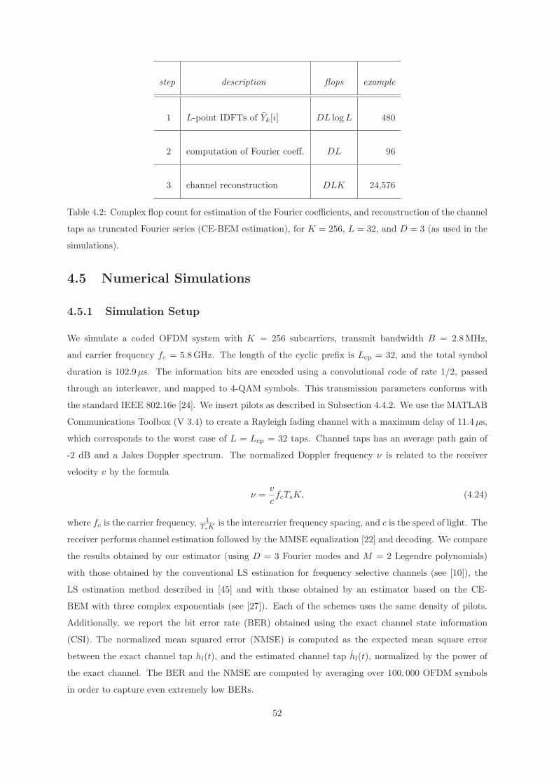
step description flops example

1 L-point IDFTs of Yk[i] DL logL 480

2 computation of Fourier coeff. DL 96

3 channel reconstruction DLK 24,576

Table 4.2: Complex flop count for estimation of the Fourier coefficients, and reconstruction of the channel

taps as truncated Fourier series (CE-BEM estimation), for K = 256, L = 32, and D = 3 (as used in the

simulations).

4.5 Numerical Simulations

4.5.1 Simulation Setup

We simulate a coded OFDM system with K = 256 subcarriers, transmit bandwidth B = 2.8MHz,

and carrier frequency fc = 5.8GHz. The length of the cyclic prefix is Lcp = 32, and the total symbol

duration is 102.9µs. The information bits are encoded using a convolutional code of rate 1/2, passed

through an interleaver, and mapped to 4-QAM symbols. This transmission parameters conforms with

the standard IEEE 802.16e [24]. We insert pilots as described in Subsection 4.4.2. We use the MATLAB

Communications Toolbox (V 3.4) to create a Rayleigh fading channel with a maximum delay of 11.4µs,

which corresponds to the worst case of L = Lcp = 32 taps. Channel taps has an average path gain of

-2 dB and a Jakes Doppler spectrum. The normalized Doppler frequency ν is related to the receiver

velocity v by the formula

ν =v

cfcTsK, (4.24)

where fc is the carrier frequency,1

TsKis the intercarrier frequency spacing, and c is the speed of light. The

receiver performs channel estimation followed by the MMSE equalization [22] and decoding. We compare

the results obtained by our estimator (using D = 3 Fourier modes and M = 2 Legendre polynomials)

with those obtained by the conventional LS estimation for frequency selective channels (see [10]), the

LS estimation method described in [45] and with those obtained by an estimator based on the CE-

BEM with three complex exponentials (see [27]). Each of the schemes uses the same density of pilots.

Additionally, we report the bit error rate (BER) obtained using the exact channel state information

(CSI). The normalized mean squared error (NMSE) is computed as the expected mean square error

between the exact channel tap hl(t), and the estimated channel tap hl(t), normalized by the power of

the exact channel. The BER and the NMSE are computed by averaging over 100, 000 OFDM symbols

in order to capture even extremely low BERs.

52

4.5.2 Results of Simulations

Figure 4.4 shows the BER and the NMSE as functions of the receiver velocity for a fixed SNR with

Eb/N0 = 20dB. Clearly, the performance deteriorates with increasing velocity. For the chosen system

parameters, the conventional LS estimation is the best of all the methods at velocities less than 113 km/h

(5.6% normalized Doppler). We note, the LS estimation is a special case of the proposed estimation

algorithm with the Fourier model order D = 1 and the Legendre model order M = 1. For rapid channel

variations occurring at velocities larger than 113 km/h, our estimator with the Fourier model order D = 3

and the Legendre model order M = 2 performs best, having an up to one order of magnitude lower BER

than that of the CE-BEM. On Figure 4.5 and Figure 4.4, we notice that the proposed algorithm gives

a BER approximately one order of magnitude greater than the one obtained using the exact CSI. The

performance of the LS method proposed in [45] is comparable to our method, but our proposed method

have much gain in complexity. We have verified experimentally, that for the Fourier model order D = 3

and the Legendre model order M = 2, the condition numbers of linear operators used for estimation of

the BEM coefficients is 1.35. The proposed method allows us to adapt the model order to the severity

of the Doppler effect for better estimation.

Figure 4.5 shows the BER and the NMSE as functions of the signal-to-noise ratio (SNR) in terms of

Eb/N0 (Eb denotes the energy per information bit, i.e. excluding energy on pilot subcarriers, and N0

is the variance of the AWGN) for a fixed receiver velocity of 300 km/h. This velocity corresponds to a

maximum Doppler shift of 1.61 kHz, which is about 14.7% of the subcarrier spacing. We note that, from

the vantage point of a stationary receiver, the Doppler effect of a moving reflector is twice as large as that

of a moving transmitter. Thus, a reflector moving with velocity 150 km/h also gives rise to a Doppler shift

of 1.61 kHz. We can see that for all these estimators, the NMSE and the BER keeps on improving with

increasing SNRs. The limit performance of each model and method will be reached finally at a very high

SNR, which might be an impractical level of additive noise. However, the BER levels of our proposed

estimator at different SNRs are significantly lower than those of the CE-BEM-based scheme, which in

turn are lower than those of the conventional LS estimation. Our scheme achieves a BER of 10−4 at

Eb/N0 = 22dB (roughly 5 dB away from the limit), the LS and the CE-BEM-based channel estimation

methods do not even achieve such low BERs. Even at a BER of 10−3, our estimator outperforms the

CE-BEM by about 3.5 dB.

4.6 Chapter Conclusions

We develop a novel, numerically stable, low-complexity channel estimator for OFDM systems, which is

reliable at high Doppler spreads. The main idea is to use a BEM with the Legendre polynomials in

order to mitigate the Gibbs phenomenon, and provide a more accurate reconstruction than a truncated

Fourier series (CE-BEM). The Legendre coefficients of the channel taps are computed from explicit

formulas involving the pilot values and the receive signal.

53

40 80 160 320 640−35

−30

−25

−20

−15

receiver velocity [km/h]

NM

SE

[dB

]

conventional CE−BEM method of [45] proposed

(a)

40 80 160 320 64010

−6

10−5

10−4

10−3

10−2

10−1

100

receiver velocity [km/h]

BE

R

conventional CE−BEM method of [45] proposed exact CSI

(b)

Figure 4.4: (a) NMSE versus receiver velocity and (b) BER versus receiver velocity for a fixed SNR of

Eb/N0 = 20dB.

54

5 10 15 20 25 30 35 40−35

−30

−25

−20

−15

Eb/N

0 [dB]

NM

SE

[d

B]

conventional CE−BEM proposed

(a)

5 10 15 20 25 30 35

10−6

10−4

10−2

100

Eb/N

0 [dB]

BE

R

conventional CE−BEM proposed exact CSI

(b)

Figure 4.5: (a) NMSE versus SNR and (b) BER versus SNR for a fixed receiver velocity of 300 km/h.

55

The conventional least-squares (LS) estimation is a method of choice for doubly-selective channels

with low Doppler spreads. Our proposed algorithm is aimed at doubly-selective channels with moderate

Doppler spreads, corresponding to reflector velocities in the range of 60−200 km/h and a carrier frequency

of 5.8GHz. The LS estimation is a special case of the proposed method with the Fourier model order

D = 1 and the Legendre model order M = 1. At higher Doppler spreads, reliable channel estimates are

obtained with higher models orders, at the expense of the transmission capacity.

56

Chapter 5

Low Complexity Equalization for

Doubly Selective Channels Modeled

by a Basis Expansion

5.1 Introduction

5.1.1 Overview

In this chapter we propose a novel equalization method for doubly selective wireless channels, whose

channel taps are represented by a Basis Expansion Model (BEM). We view the action of such a channel

in the time domain as a sum of product-convolution operators created from the basis functions and the

BEM coefficients, see Section 3.8. We perform iterative equalization with the GMRES and the LSQR

algorithms, as described in Section 2.7, which utilize the product-convolution structure without ever

explicitly creating the wireless channel matrix. In an OFDM transmission with K subcarriers, each

iteration of GMRES or LSQR requires only O(K logK) complex flop and O(K) memory. Additionally,

for a considerable range of Doppler shift, we dramatically accelerate convergence of both GMRES and

LSQR by using single tap-equalizer as a preconditioner. Thanks to preconditioning, we typically need 3

to 6 iterations for convergence, depending on the Doppler shift in the channel, and the method employed.

Consequently, the proposed equalization amounts to the single-tap equalization combined with GMRES

or LSQR iterations in order to resolve Inter Carrier Interference (ICI). In numerical simulations of a

WiMAX-like system in doubly selective channels with severe Doppler shifts, the proposed equalizer in

combination with presently available estimation algorithms outperforms the conventional equalizer by an

order of magnitude in BER. Our approaches dose not use any statistical information about the wireless

channel.

1Part of this chapter is submitted for a journal publication

57

5.1.2 Motivation and Previous Work

In the last two decades, there has been a steady increase in the number of applications utilizing rapidly

varying wireless communication channels. Such channels occur due to user mobility in the systems like

DVB-T and WiMAX, which have been originally designed for fixed receivers. Rapidly varying channels

exhibit significant intercarrier interference (ICI), which has to accounted for by any equalization method.

Moreover, several applications have short symbol durations, and therefore require fast equalization algo-

rithms. One such example is the mobile WiMAX with a symbol duration of 102.9 µs according to IEEE

standard 802.16e.

To illustrate our equalization method, we consider a system with orthogonal frequency-division mul-

tiplexing (OFDM), which is commonly used for frequency multiplexing in multi-carrier (MC) communi-

cation systems, see Section 2.3 for more detail. Main advantages of OFDM are robustness to multipath

interference and an efficient use of bandwidth [5]. Specific applications include mobile WiMAX (IEEE

802.16e), WAVE (IEEE 802.11p), and 3GPP’s UMTS Long-Term Evolution (LTE).

In this chapter, we assume that the wireless channel is represented in terms of a basis expansion model

(BEM), which approximates the channel taps by linear combinations of prescribed basis functions, see

[49, 15, 54, 45, 46, 42]. In this context, channel estimation amounts to an approximate computation of

coefficients for the basis functions. Several methods for estimation and equalization with the BEM have

been proposed. The complex exponential BEM (CE-BEM) [49, 15, 9, 20] uses a truncated Fourier series,

and the resulting approximate channel matrix is banded in the frequency domain. A more suitable

exponential basis – complex exponentials oversampled in the frequency domain – is employed by the

generalized CE-BEM (GCE-BEM) [29]. A basis of discrete prolate spheroidal wave functions is discussed

in [54, 53]. Finally, the polynomial BEM (P-BEM) is presented in [6], [21]. For channels varying on the

scale of one OFDM symbol, pilot-aided channel estimation is studied in [45]. Definitive references on

pilot-aided transmission in doubly-selective channels are [26, 27].

There exist several methods for estimating the BEM coefficients of doubly selective channel taps,

especially with an OFDM transmission setup, see [45, 46, 42, 21], and Chapter 4. Usually, the wireless

channel matrix is reconstructed from estimated BEM coefficients and subsequently used in equalization.

However, with severe ICI the conventional single-tap equalization in the frequency domain is unreliable,

see [36, 30, 38]. Several other approaches have been proposed to combat ICI in transmissions over

rapidly varying channels. For example, [8] presents minimum mean-square error (MMSE) and successive

interference cancellation equalizers, which use all subcarriers simultaneously. Alternatively, using only

a few subcarriers in equalization amounts to approximating the frequency-domain channel matrix by a

banded matrix, and has been exploited for equalizer design, see [47, 37]. ICI-shaping, which concentrates

the ICI power within a small band of the channel matrix, is described in [47, 41]. A low-complexity time-

domain equalizer based on the LSQR algorithm is introduced in [22].

58

5.1.3 Contributions

In this chapter we propose a fast and accurate equalization method for communication systems in doubly-

selective wireless channels, which uses only estimated BEM coefficients and the receive signal. The

method represents the time-domain channel matrix as a sum of product-convolution operators [49, 15]

without ever constructing the channel matrix itself. For contemporary and upcoming application, where

the number of discrete channel taps L is a fraction of number of subcarriers K, like L = K/8,K/16

for mobile WiMAX (IEEE 802.16e), an explicit reconstruction of the channel matrix requires O(K2)

memory and O(K2) flops, which is prohibitive in several practical applications. The product operators

are diagonal matrices with the basis functions as diagonals. The convolution operators, which act as

time-invariant filters, are formed by zero-padding the BEM coefficients. This particular structure of

the channel matrix allows us to equalize the signal with a very low complexity by classical iterative

methods, namely GMRES [39] and LSQR [34]. Additionally, we significantly accelerate convergence of

both GMRES and LSQR by preconditioning them with the single-tap (ST) equalizer. On the whole, our

proposed equalization method amounts to the single-tap equalization combined with GMRES or LSQR

iterations in order to resolve ICI.

Our main contributions can be summarized as follows:

• We propose to use the standard iterative methods GMRES and LSQR for stable regularized equal-

ization without creating the full channel matrix. In an OFDM setup with K subcarriers, each

iteration requires O(K logK) flops and O(K) memory.

• We propose the single-tap equalizer as an efficient preconditioner for both GMRES and LSQR.

For illustration, we use an OFDM system in doubly-selective channels. In computer simulations of

a WiMAX-like system in doubly-selective channels, the proposed equalization method in combination

with presently available estimation algorithms requires only a few iterations to outperform the conven-

tional equalizer by an order of magnitude in BER. We emphasize that, we do not consider any banded

approximation of the channel matrix in the frequency domain.

This chapter is organized as follows. In Section II, we introduce our transmission setup and an

assumed model for the wireless channel. The proposed iterative equalization methods and preconditioners

are described in Section III. We present our simulation results in Section IV, and chapter conclusions in

Section V.

5.2 System Model

5.2.1 Transmission Model

To illustrate our equalization method we consider an OFDM setup in doubly selective channels. We

consider an equivalent baseband representation of a single-antenna OFDM system with K subcarriers.

Our method can be adapted to a MIMO setup in a straightforward manner. We assume a sampling

59

period of Ts = 1/B, where B denotes the transmit bandwidth. A cyclic prefix of length Lcp is used in

every OFDM symbol. We choose Lcp so large, that LcpTs exceeds the channel’s maximum delay, so that

we avoid inter-symbol interference (ISI). Consequently, throughout this chapter we deal with one OFDM

symbol at a time, and all further models and formulations refer to one OFDM symbol.

Each subcarrier is used to transmit a symbolA[k] (k = 0, . . . ,K−1) from a finite symbol constellation

(e.g. 4QAM, PSK, 64QAM). Depending on the transmission setup, some of these symbols serve as pilots

values for channel estimation. The OFDMmodulator uses the Inverse Discrete Fourier Transform (IDFT)

to map the frequency-domain transmit symbols A[k] into the time-domain transmit signal x[n]

x[n] =1√K

K−1∑

k=0

A[k] e2πnkK , (5.1)

n = −Lcp, . . . ,K−1.

After discarding the cyclic prefix at the receiver, the receive signal satisfies

y[n] =

L−1∑

l=0

hl[n]x[n− l] +w[n], n = 0, . . . ,K − 1. (5.2)

Here, w[n] denotes complex additive noise of variance N0, hl[n] is the complex channel tap associated

with delay the l, and L is the channel length (maximum discrete-time delay). Consequently, the chan-

nel’s maximum delay equals (L−1)Ts. For simplicity, we make the worst-case assumption L = Lcp.

Equivalently, the transmit-receive relation (5.2) can be written as

y = Hx+w, (5.3)

where H is the time-domain channel matrix.

The OFDM demodulator at the receiver’s end performs the following tasks with the sampled time-

domain receive signal: channel estimation, equalization, demodulation by means of the DFT, quantiza-

tion, decoding and deinterleaving. In this chapter, we assume that a channel estimate in terms of the

BEM coefficients is already provided. In the next section, we develop methods for equalization of the

receive signal using the estimated BEM coefficients.

5.2.2 Wireless Channel Representation with BEM

We assume the basis expansion model (BEM) for channel taps. With the BEM, each channel tap

hl is modeled as a linear combination of suitable basis functions, see Section 3.8. Several bases are

proposed in literature, including complex exponentials [49, 15, 9, 20], complex exponentials oversampled

in the frequency domain [29], discrete prolate spheroidal functions [53], polynomials [6], in particular the

Legendre polynomials in Chaper 4.

With specific set of basis functions, the channel tap hl is represented as follows

hl[n] =M−1∑

m=0

blm Bm[n] , l = 0, . . . , L−1, (5.4)

60

where blm is the mth basis coefficient of the lth channel tap, Bm is the mth basis function, and M is the

BEM model order. Relation (5.4) is correct up to a modeling error, which can be reduced by increasing

the model order M . On the other hand, in pilot-based estimation methods increasing M decreases the

transmission capacity.

Combining (5.2) and (5.4), the time-domain receive signal y is expressed as

y[n] =

L−1∑

l=0

(M−1∑

m=0

blm Bm[n]

)x[n− l] +w[n], (5.5)

where n = 0, . . . ,K−1, and w is an additive error, which consists of random noise and a systematic

modeling error.

5.2.3 Equivalence of the BEM and the Product-Convolution Representation

Changing the order of summation in equation (5.5), we obtain

y[n] =

M−1∑

m=0

Bm[n]︸︷︷︸product

(L−1∑

l=0

blm x[n− l]

)

︸︷︷︸convolution︸︷︷︸

sum of product-convolutions

+w[n]. (5.6)

Equivalently, the time-domain channel matrix H can be expressed as a sum of product-convolutions as

follows:

H =M−1∑

m=0

PmCm, (5.7)

where Pm is a diagonal matrix with Pm(i, i) equal to Bm(i), and Cm is a circulant matrix representing

the cyclic convolution with the mth set of BEM coefficients {b·m}.

5.3 Equalization

5.3.1 Iterative Equalization Methods

It is well-known, that the conventional single tap equalization in the frequency domain is inaccurate for

doubly selective channels with severe ICI, see [36, 30, 38]. Direct methods, like the MMSE equalization,

are impractical because of a high computational complexity and an excessive memory usage. Low-

complexity methods, that rely on approximation by a banded matrix in the frequency-domain, correct

only relatively modest ICI.

In their stead, we propose equalization with two standard iterative methods for the approximate

solution of linear systems, namely GMRES [39] and LSQR [34]. They are both Krylov subspace methods,

i.e. each approximate solution is sought within an increasing family of Krylov subspaces. Specifically, at

the ith iteration GMRES constructs an approximation within the subspace

K(H,y, i) = Span{y,Hy,H2y, . . . ,H(i−1)y

}, (5.8)

61

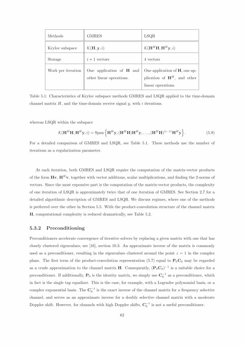
Methods GMRES LSQR

Krylov subspace K(H,y, i) K(HHH,HHy, i)

Storage i+ 1 vectors 4 vectors

Work per iteration One application of H and

other linear operations.

One application of H, one ap-

plication of HH , and other

linear operations.

Table 5.1: Characteristics of Krylov subspace methods GMRES and LSQR applied to the time-domain

channel matrix H, and the time-domain receive signal y, with i iterations.

whereas LSQR within the subspace

K(HHH,HHy, i) = Span{HHy, (HHH)HHy, . . . , (HHH)(i−1)HHy

}. (5.9)

For a detailed comparison of GMRES and LSQR, see Table 5.1. These methods use the number of

iterations as a regularization parameter.

At each iteration, both GMRES and LSQR require the computation of the matrix-vector products

of the form Hv, HHv, together with vector additions, scalar multiplications, and finding the 2-norms of

vectors. Since the most expensive part is the computation of the matrix-vector products, the complexity

of one iteration of LSQR is approximately twice that of one iteration of GMRES. See Section 2.7 for a

detailed algorithmic description of GMRES and LSQR. We discuss regimes, where one of the methods

is preferred over the other in Section 5.5. With the product-convolution structure of the channel matrix

H, computational complexity is reduced dramatically, see Table 5.2.

5.3.2 Preconditioning

Preconditioners accelerate convergence of iterative solvers by replacing a given matrix with one that has

closely clustered eigenvalues, see [16], section 10.3. An approximate inverse of the matrix is commonly

used as a preconditioner, resulting in the eigenvalues clustered around the point z = 1 in the complex

plane. The first term of the product-convolution representation (5.7) equal to P0C0 may be regarded

as a crude approximation to the channel matrix H. Consequently, (P0C0)−1 is a suitable choice for a

preconditioner. If additionally, P0 is the identity matrix, we simply use C−10 as a preconditioner, which

in fact is the single tap equalizer. This is the case, for example, with a Legendre polynomial basis, or a

complex exponential basis. The C−10 is the exact inverse of the channel matrix for a frequency selective

channel, and serves as an approximate inverse for a doubly selective channel matrix with a moderate

Doppler shift. However, for channels with high Doppler shifts, C−10 is not a useful preconditioner.

62

In order to introduce preconditioner, we introduce a new variable

x = C0x, (5.10)

and substitute into equation (5.3) in the following manner

y = Hx+w (5.11)

= HC−10 C0x+w (5.12)

= HC¯−10 x+w (5.13)

= Hx+w, (5.14)

where H = HC−10 . In view of equation (5.7), we have

H = HC−10 (5.15)

=M−1∑

m=0

PmCmC−10 (5.16)

=M−1∑

m=0

PmCm, (5.17)

where Cm = CmC−10 for m = 0, 1, · · · ,M − 1. Clearly, the transformed time-domain channel matrix H

is also a sum of product-convolutions, so both matrices H and H¯

Hcan be applied at a cost O(K logK).

Algebraically, replacing equation (5.3) by equation (5.14) is classified as right preconditioning. For some

bases, e.g. that of discrete prolates, P0 is not a constant. In such cases, one should use both left and

right preconditioning, see Section 2.7 for details.

Eigenvalues of a representative time domain channel matrix H, and its preconditioned version H =

HC−10 , are shown in Fig. 5.1. We notice that the eigenvalues of the preconditioned matrix H are clustered

near the point z = 1 in the complex plane. We have observed experimentally, that preconditioning with

ST equalizer is not effective for channels whose Doppler shift exceeds 25% of the intercarrier frequency

spacing. Such channels are far away from being frequency selective, and ST equalizer is not a reliable

approximate inverse.

5.4 Description of the Algorithm

5.4.1 Decomposition of Channel Matrix

The proposed equalization uses only the BEM coefficients of the channel taps and the time-domain receive

signal. We assume that estimates of the BEM coefficients are known, for example they are provided by

one of the estimation methods mentioned in the introduction. In this subsection, we do mathematical

derivations, which helps to formulate the algorithm for equalization as presented in the next subsection.

It is well-known, for example see [16] (p. 202), that conjugating a circulant matrix by the discrete

Fourier transform (DFT) results in a diagonal matrix. The cyclic convolution matrices Cm are thus

63

−2 −1.5 −1 −0.5 0 0.5 1 1.5 2−2

−1.5

−1

−0.5

0

0.5

1

1.5

2

Figure 5.1: Eigenvalues of the time domain channel matrix with a Doppler shift equal to 17% of the

inter carrier frequency spacing without preconditioning ’◦’, and with preconditioning ’•’.

expressed as

Cm = FHDmF , m = 0, . . . ,M−1, (5.18)

where Dm are diagonal matrices, and F is the matrix of the DFT in K dimensions. The diagonal of the

matrix Dm coincides with the DFT of the BEM coefficients b·m zero-padded to length K,

Dm(i, i) =(F[b·m, 0, . . . , 0]T

)(i), (5.19)

for i = 1, . . . ,K and (·)T denote the transpose operation.

Substituting relation (5.18) into equation (5.16), we get

H =

M−1∑

m=0

PmFHDmFFHD−10 F (5.20)

=

M−1∑

m=0

PmFHDmF (5.21)

where

Dm = DmD−10 (5.22)

is a diagonal matrix. Similarly, substituting relation (5.18) into equation (5.10), we get

x = C0x = FHD0Fx. (5.23)

Using the expression for H, see equation (5.21), we express the time domain receive signal y, see equa-

tion (5.14), in the following form

y =

(M−1∑

m=0

PmFHDmF

)x+w. (5.24)

64

5.4.2 Algorithm

The proposed equalization algorithm in the time domain is based on equation (5.24), and can be sum-

marized as follows: given the time-domain receive signal y and the BEM coefficients blm, we solve for

x using iterative solvers GMRES or LSQR, and then we approximate A with D−10 Fx. Specifically, we

perform the following steps:

Step 1 Compute the diagonal matrices Dm from the BEM coefficients blm, see equation (5.19).

Step 2 Compute the diagonal matrices Dm = DmD−10 , see equation (5.22).

Step 3 Solve (5.24) for x using GMRES or LSQR.

Step 4 Approximate A as D−10 Fx, see equation (5.29).

Step 5 Quantize according to the alphabet used (4QAM, PSK etc.).

We employ Step 2 only if we do preconditioning, otherwise, we take Dm equal toDm. A similar algorithm

for equalization in the frequency domain can be formulated using equation (5.28). Equalization in the

time and in the frequency domain give identical errors, because they are related by a unitary operator.

In the frequency domain, equation (5.24) has the form

Y = Fy (5.25)

= F

(M−1∑

m=0

PmFHDmF

)x+W, (5.26)

= F

(M−1∑

m=0

PmFHDm

)FFHD0Fx+W, (5.27)

= F

(M−1∑

m=0

PmFHDm

)

︸︷︷︸ICI

D0︸︷︷︸FS

A+W, (5.28)

where, W is the noise in the frequency domain, and

A = Fx = D−10 Fx (5.29)

is the frequency-domain transmit signal as used in equation (5.1), and Y is the receive signal in the

frequency domain. Equation (5.28) demonstrates that doubly selective frequency-domain channel matrix

is the product of a purely frequency selective (FS) operator D0, and an operator modeling ICI.

5.4.3 Computational Complexity

In this subsection we report operation counts of equalization of one OFDM symbol. We consider the

diagonal matrices Pm to be precomputed. Computation of diagonal matrices Dm from the BEM co-

efficients in Step 1 requires O(MK logK) operations. Whenever preconditioning is used, we perform

Step 2 (creation of the diagonal matrices Dm), which requires O(MK) operations. In Step 3, we solve

65

step description complex flop count example

1 computingDm from BEM coeff. blm MK logK 4096

2 computing Dm from Dm (M − 1)K 256

3 solving x iteratively using:

a. GMRES (i+1)MK logK+(i2+3i+Mi+M)K+5i2+12i+7 23128

b. LSQR (2i+1)MK logK +(10i+3+2Mi+2M)K+14i+1 41259

4 equalizing A as D−10 F x K logK +K 2304

5 quantizing to symbol constellation K 256

Table 5.2: Complex flop count for the proposed algorithm per OFDM symbol. Specific values are reported

for K = 256 subcarriers, BEM model order M = 2 , number of iterations i = 3 of GMRES or LSQR (as

used in the simulations).

for x using iterative methods GMRES or LSQR, which requires O(K logK) operations per iteration.

Number of iterations depends on the Doppler shift in the wireless channel and the equalization method.

Typically for LSQR it does not exceed 14 without preconditioning, and dosenot exceed 6 with precondi-

tioning, for a normalized Doppler around 15%. On the other hand GMRES with preconditioning takes 3

iterations to reach its best performance at around 15% normalized Doppler. In Step 4, we compute the

frequency-domain transmit signal A from x using equation (5.29), which requires O(K logK) operations.

In Step 5, we quantize the signal A according to the alphabet used at the cost of O(K) operations. A

detailed breakdown of computational complexity is provided in Table 5.2.

5.4.4 Memory

The equalization process begins with the time-domain receive signal y and the BEM coefficients blm,

which are stored as K and ML floating point complex numbers, respectively. Pm and Dm are diagonal

matrices, which are stored as K complex numbers each. The matrix-vector multiplications required by

GMRES and LSQR are done using pointwise multiplications and the FFT-s of size K, see equation

(5.21). After the ith iteration GMRES requires storing i + 1 vectors of length K, while LSQR requires

storing four vectors of length K. The storage of GMRES can be lowered down by using an intermediate

restart of the algorithm, but that is not necessary as we do not need more that 3 iterations especially

GMRES for. Thus the proposed algorithm requires O(K) in memory.

66

5.5 Numerical Simulations

5.5.1 Simulation Setup

Our transmission setup conforms to the IEEE 802.16e specifications. We simulate a coded OFDM

system with K = 256 subcarriers, utilizing B = 2.8MHz of bandwidth at a carrier frequency of fc =

5.8GHz. We use a cyclic prefix of length Lcp = 32 in order to avoid ISI. Consequently, the sampling

period is Ts = 1/B = 0.357µs, and the symbol duration is (K + Lcp)Ts = (256 + 32) × 0.357µs =

102.9µs. The information bits are encoded using a convolutional code of rate 1/2, passed through an

interleaver, and mapped to 4-QAM symbols. For experiments with the estimated BEM coefficients, we

use a frequency domain Kronecker delta (FDKD) pilot arrangement in each OFDM symbol, as described

in [26], Chapter 4. The pilots are only used for estimation of the BEM coefficients, and do not have

any influence on the proposed equalization algorithm. Experiments with exact channel state information

(CSI) do not use pilots in transmission.

We simulate a wide sense stationary uncorrelated scattering (WSSUS) Rayleigh fading channel with

a maximum delay of 11.4µs, which corresponds to the worst case when L = Lcp = 32 taps. Each tap

has an average path gain of -2 dB and a Jakes Doppler spectrum. We filter the simulated transmit signal

through the channel with varying maximum Doppler shifts. The maximum Doppler shift νmax is related

to the receiver velocity v by the formula

νmax =fcv

c, (5.30)

where c is the speed of light. To the signal filtered through the channel, we add additive white Gaussian

noise (AWGN) of varying energy per data bit to noise spectral density (Eb/N0). The values of νmax, v,

Eb/N0 are reported for all the experiments. The channel is simulated using the MATLAB Communication

Toolbox (ver. 3.4).

At the receiver, we first compute the BEM coefficients. Specifically, in our experiments we use the

basis of the Legendre polynomials, as described in Chapter 4. In experiments with estimated channel

taps, we use the algorithm described in Chapter 4 for estimation of the BEM coefficients. In experiments

with the exact channel matrix, we compute the BEM coefficients by projecting the channel taps on the

basis functions. Subsequently, we equalize the receive signal using the proposed algorithm. Finally, the

equalized signal is quantized and decoded using the BCJR algorithm and deinterleaved. As a measure

of performance, we report the bit error rate (BER) averaged over 100, 000 OFDM symbols.

5.5.2 Discussion of Results

First, we study the dependence of the BER on the number of iterations of GMRES and LSQR, with and

without preconditioning. In the case of GMRES, we only present the results with preconditioning, since

without preconditioning GMRES needs approximately K iterations to achieve a useful BER. We note

that one iteration of LSQR requires approximately twice as many flop as that of GMRES, see Table 5.2

for details. Figures 5.2, 5.3, and 5.4 show the BER as a function of the number of iterations at the

67

0 5 10 15 2010

−6

10−5

10−4

10−3

number of iterations

BE

R

STprecond. GMRESLSQRprecond. LSQR

Figure 5.2: The BER as a function of the number of iterations at the velocity of 175 km/h (low Doppler

Shift) and the SNR of Eb/N0 = 20dB using exact CSI.

receiver velocities of 175, 300 and 550 km/h, respectively. We consider resulting Doppler at these three

receiver velocities as examples of low, moderate, and high Doppler shift in wireless channel. The additive

noise in the channel is simulated for a fixed SNR of Eb/N0 = 20dB. The exact CSI is used in all these

experiments. The BER at iteration number zero corresponds to the single-tap (ST) equalization, which

is shown for comparison.

Fig. 5.2 presents results for the receiver velocity of 175 km/h, which corresponds to a Doppler shift

of 0.94 kHz, or about 8.6% of the subcarrier spacing. The BER of the ST equalization amounts to

7.8 e–5, while that of preconditioned GMRES decreases from 3.1 e–5 after one iteration, to 2.3 e–5 after

3 iterations. The BER of LSQR decreases from 6.5 e–4 after one iteration to 1.6 e–5 after 16 iterations.

The BER of preconditioned LSQR decreases from 4.7 e–5 after one iteration to 7.8 e–6 after 4 iterations.

Fig. 5.3 presents results for the receiver velocity of 300 km/h, which corresponds to a Doppler shift of

1.61 kHz, or about 14.7% of the subcarrier spacing. The BER of the ST equalization amounts to 7.4 e–4,

while that of preconditioned GMRES is 3.7 e–4 after one iteration and slowly increasing afterwards. The

BER of LSQR decreases from 3.1 e–3 after one iteration to 1.2 e–5 after 15 iterations. The BER of

preconditioned LSQR decreases from 5.6 e–4 after one iteration to 3.9 e–5 after 6 iterations.

Fig. 5.4 presents results for the receiver velocity of 550 km/h, which corresponds to a Doppler shift of

2.95 kHz, or about 27% of the subcarrier spacing. The BER of the ST equalization amounts to 1.9 e–2,

while that of preconditioned GMRES is 1.2 e–2 after one iteration and slowly increasing afterwards.

The BER of LSQR decreases from 1.7 e–2 after one iteration to 1.5 e–4 after 12 iterations. The BER

of preconditioned LSQR decreases from 1.9 e–2 after one iteration to 6.8 e–4 after 9 iterations. In this

scenario, LSQR is the method of choice. Preconditioning with single tap equalizer does not help any

more, because the channel is intrinsically doubly-selective.

68

0 5 10 15 2010

−5

10−4

10−3

10−2


BE

R


Figure 5.3: The BER as a function of the number of iterations at the velocity of 300 km/h (moderate

Doppler shift) and the SNR of Eb/N0 = 20dB using exact CSI.

All iterative methods in Figures 5.2, 5.3, and 5.4 display the phenomenon known as semi-convergence.

Specifically, the first few iterations provide approximations of increasing accuracy, as seen by the decreas-

ing BERs. The subsequent iterations do not further improve the resolution, and sometimes even amplify

the ambient noise, as evidenced by the slowly increasing BERs.

Fig. 5.5, 5.6, and 5.7 show the dependence of the BER on the SNR expressed in terms of the energy

per bit to noise spectral density ratio Eb/N0 for channels simulated with the receiver speed of 175 km/h,

300 km/h, and 550 km/h. We present our results for channels estimated using a pilot-aided method

described in Chapter 4, and also the results obtained with the exact channel matrix as a benchmark.

Fig. 5.5(a) and 5.5(b) show the BER with the exact and estimated CSI, respectively, corresponding to

the receiver velocity of 175 km/h, or 8.6% of the subcarrier spacing. We use 3 iterations of preconditioned

GMRES, 14 iterations of LSQR, and 8 iterations of preconditioned LSQR. The observed BERs saturate

at high SNRs. Specifically, with exact CSI, the ST equalization saturates at the BER of 2.2 e–5, the

preconditioned GMRES at 6.5 e–6, LSQR at 1.9 e–6 and preconditioned LSQR at 2.0 e–7. With estimated

CSI, the saturation levels are 1.3 e–5 for the ST equalization, 6.1 e–6 for preconditioned GMRES, 9.4 e–7

for LSQR, and 9.4 e–7 for preconditioned LSQR.

Fig. 5.6(a) and 5.6(b) show the BER with the estimated and exact CSI, respectively, corresponding to

the receiver velocity of 300 km/h, or 14.7% of the subcarrier spacing. We use 10 iterations of LSQR, and 6

iterations of preconditioned LSQR. For such high Doppler shifts, the BER of GMRES is indistinguishable

from that of the ST equalization, so only the first one is plotted. The observed BERs saturate at high

SNRs. Specifically, with exact CSI, the ST equalization saturates at the BER of 6.1 e–4, LSQR at 2.2 e–5

and preconditioned LSQR at 1.2 e–5. With estimated CSI, the saturation levels are 3.1 e–3 for the ST

equalization, 1.1 e–5 for LSQR, and 2.6 e–5 for preconditioned LSQR.

69

Fig. 5.7(a) and 5.7(b) show the BER with the estimated and exact CSI, respectively, corresponding

to the receiver velocity of 550 km/h, or 27% of the subcarrier spacing. We use 14 iterations of LSQR,

and 14 iterations of preconditioned LSQR. The observed BERs saturate at high SNRs. Specifically, with

exact CSI, the ST equalization saturates at the BER of 1.7 e–2, LSQR at 9.4 e–5 and preconditioned

LSQR at 4.1 e–4. With estimated CSI, the saturation levels are 5.9 e–2 for the ST equalization, 1.1 e–4

for LSQR, and 5.2 e–4 for preconditioned LSQR.

The performance of the equalization method using estimated BEM coefficients, demonstrates the

feasibility of the proposed equalization method in combination with presently available BEM estimation

algorithms.

5.6 Chapter Conclusions

In this chapter, we present a method for using the BEM coefficients of wireless channel taps directly for

equalization without ever creating the channel matrix. We focus on doubly selective channels modeled

by the basis expansion model (BEM) as a sum of product convolution operators. We perform iterative

equalization with GMRES and LSQR, and test the proposed equalization method on an OFDM system.

The product convolution structure of the channel matrix allow the computation of the matrix-vector

products with O(MK log K) operations, where M is BEM model order. We demonstrate how to use

single tap equalizer for preconditioning. Our simulation result show that the preconditioning dramati-

cally accelerates the convergence of both GMRES and LSQR. Consequently, the proposed equalization

algorithm amounts to the single tap equalization combined with GMRES or LSQR iterations in order to

resolve the ICI.

We observe that convergence of GMRES is extremely slow, where as preconditioned GMRES is fast,

but effective only for doubly selective channels with moderate Doppler shift. Preconditioned LSQR is

very effective for doubly selective channels with moderate to high Doppler shifts. We have observed

experimentally, that preconditioning with ST is not effective for channels whose Doppler shift exceeds

25% of the intercarrier frequency spacing. Such channels are far away from being frequency selective,

and the single-tap equalizer is not a reliable approximate inverse.

70

0 5 10 15 2010

−4

10−3

10−2

10−1


BE

R


Figure 5.4: The BER as a function of the number of iterations at the velocity of 550 km/h (high Doppler

Shift) and the SNR of Eb/N0 = 20dB using exact CSI.

71

0 5 10 15 20 25 30 35 4010

−7

10−6

10−5

10−4

10−3

10−2

10−1

100

Eb/N

0 [dB]

BE

R

STprecond. GMRES (3 iter.)LSQR (14 iter.)precond. LSQR (8 iter.)

(a) Using exact CSI.

0 5 10 15 20 25 30 35 4010

−7

10−6

10−5

10−4

10−3

10−2

10−1

100

Eb/N

0 [dB]

BE

R

STprecond. GMRES (3 iter.)LSQR (14 iter.)precond. LSQR (8 iter.)

(b) Using estimated CSI.

Figure 5.5: The BER vs. the SNR expressed as Eb/N0 at the velocity of 175 km/h (low Doppler Shift).

72

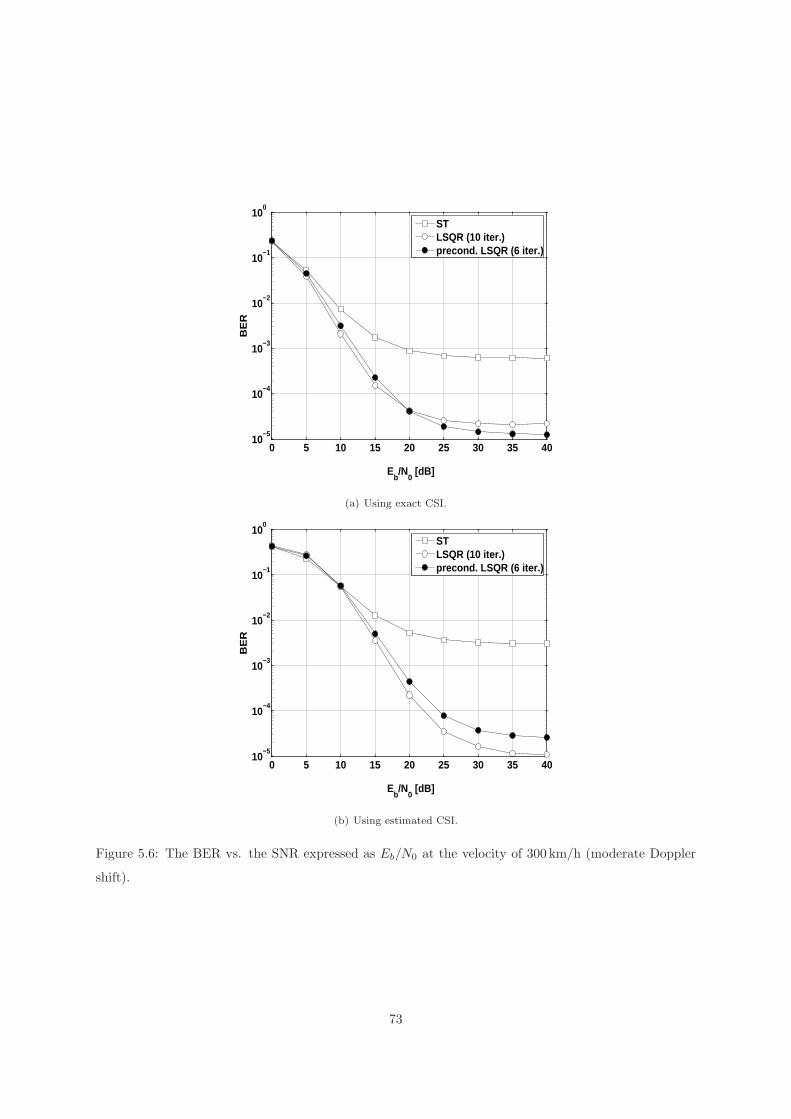
0 5 10 15 20 25 30 35 4010

−5

10−4

10−3

10−2

10−1

100

Eb/N

0 [dB]

BE

R

STLSQR (10 iter.)precond. LSQR (6 iter.)


0 5 10 15 20 25 30 35 4010

−5

10−4

10−3

10−2

10−1

100

Eb/N

0 [dB]

BE

R



Figure 5.6: The BER vs. the SNR expressed as Eb/N0 at the velocity of 300 km/h (moderate Doppler

shift).

73

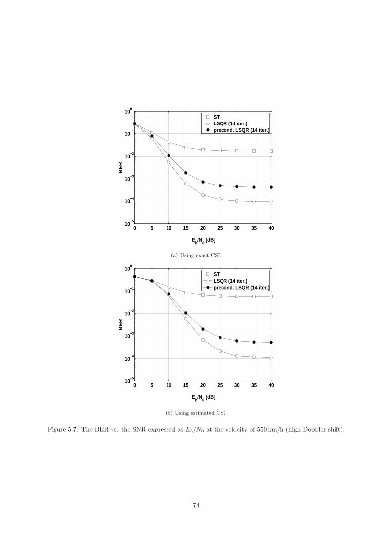
0 5 10 15 20 25 30 35 4010

−5

10−4

10−3

10−2

10−1

100

Eb/N

0 [dB]

BE

R



0 5 10 15 20 25 30 35 4010

−5

10−4

10−3

10−2

10−1

100

Eb/N

0 [dB]

BE

R



Figure 5.7: The BER vs. the SNR expressed as Eb/N0 at the velocity of 550 km/h (high Doppler shift).

74

Conclusions

In this dissertation we address problems of wireless channel estimation and equalization, for transmission

using OFDM setup through rapidly varying wireless channels. We propose an efficient low complexity

method for wireless channel estimation using a Basis Expansion Model for the wireless channel taps.

Furthermore, we propose a low complexity algorithm for equalization, which uses the estimated BEM

coefficients directly without creating the channel matrix. With L discrete channel taps, the proposed es-

timation method requires O(L logL) in operations, and O(L) in memory, Whereas previously published

methods requires O(L2) in complexity and memory. With K OFDM subcarriers, the proposed equal-

ization method require O(K logK) in operations and O(K) in memory. Computer simulation based on

the standard IEEE 802.16e shows the effectiveness of the proposed methods.

75

76

Bibliography

[1] M. Abramowitz and I. Stegun. Handbook of Mathematical Functions. Dover, New York, 1965.

[2] L. Bahl, J. Cocke, F. Jelinek, and J. Raviv. Optimal decoding of linear codes for minimizing symbol

error rate (corresp.). IEEE Transactions on Information Theory, 20(2):284–287, March 1974.

[3] P. Bello. Characterization of Randomly Time-Variant Linear Channels. IEEE Trans. Comm.,

11:360–393, 1963.

[4] P. Bello. Time-frequency duality. IEEE Transactions on Information Theory, 10(1):18–33, January

1964.

[5] J. A. C. Bingham. Multicarrier modulation for data transmission: an idea whose timehas come.

IEEE Communications Magazine, 28(5):5–14, May 1990.

[6] D. K. Borah and B. T. Hart. Frequency-selective fading channel estimation with a polynomial

time-varying channel model. 47(6):862–873, June 1999.

[7] J. P. Boyd. Chebyshev and Fourier Spectral Methods. Courier Dover, second revised edition, 2001.

[8] Yang-Seok Choi, P. J. Voltz, and F. A. Cassara. On channel estimation and detection for multicarrier

signals in fast and selective Rayleigh fading channels. IEEE Transactions on Communications,

49(8):1375–1387, August 2001.

[9] H. A. Cirpan and M. K. Tsatsanis. Maximum likelihood blind channel estimation in the presence

of Doppler shifts. IEEE Trans. Signal Processing, 47(6):1559–1569, June 1999.

[10] S. Colieri, M. Ergen, A. Puri, and Bahai A. A study of channel estimation in OFDM systems. In

Vehicular Technology Conference, 2002. Proceedings. VTC 2002-Fall. 2002 IEEE 56th, volume 2,

pages 894–898, September 2002.

[11] James W. Demmel. Applied Numerical Linear Algebra. SIAM, Society for Industrial and Applied

Mathematics, 1997.

[12] T. Driscoll and B. Fornberg. A Pade-based algorithm for overcoming the Gibbs phenomenon. Numer.

Algorithms, 26(1):77–92, 2001.

77

[13] O. Edfors, M. Sandell, J.-J. van de Beek, S.K. Wilson, and P.O. Borjesson. OFDM channel estima-

tion by singular value decomposition. Communications, IEEE Transactions on, 46(7):931–939, Jul

1998.

[14] N. Gallagher, G. Wise, and J. Allen. A novel approach for the computation of Legendre polyno-

mial expansions. Acoustics, Speech, and Signal Processing , IEEE Transactions on, 26(1):105–106,

February 1978.

[15] G. B. Giannakis and C. Tepedelenlioglu. Basis expansion models and diversity techniques for blind

identification and equalization of time-varying channels. Proceedings of the IEEE, 86(10):1969–1986,

October 1998.

[16] Gene Golub and Charles F. van Loan. Matrix Computations. 3rd ed. The Johns Hopkins University

Press, 3rd ed. edition, 1996.

[17] D. Gottlieb and C.-W. Shu. On the Gibbs phenomenon and its resolution. SIAM Review, 39(4):644–

668, 2003.

[18] I. S. Gradshteyn and I. M. Ryzhik. Table of Integrals, Series, and Products. Academic Press, 7

edition, 2007.

[19] Karlheinz Grochenig. Foundations of Time-Frequency Analysis. Appl. Numer. Harmon. Anal.

Birkhauser Boston, 2001.

[20] M. Guillaud and D. T. M. Slock. Channel modeling and associated inter-carrier interference equal-

ization for OFDM systems with high Doppler spread. In Acoustics, Speech, and Signal Processing,

2003. Proceedings. (ICASSP ’03). 2003 IEEE International Conference on, volume 4, pages 237–40,

April 2003.

[21] T. Hrycak, S. Das, G. Matz, and H. G. Feichtinger. Practical estimation of rapidly varying channels

in OFDM systems with the BEM. Submitted, 2009.

[22] T. Hrycak and G. Matz. Low-complexity time-domain ICI equalization for OFDM communications

over rapidly varying channels. In Fortieth Annual Asilomar Conference on Signals, Systems, and

Computers, Pacific Grove, CA, USA, October 2006.

[23] Meng-Han Hsieh and Che-Ho Wei. Channel estimation for OFDM systems based on comb-type pilot

arrangement in frequency selective fading channels. IEEE Transactions on Consumer Electronics,

44(1):217–225, February 1998.

[24] IEEE Draft Std 802.16e/D7. Draft IEEE Standard for Local and Metropolitan Area Networks Part

16: Air Interface for Fixed and Mobile Broadband Wireless Access Systems, 2005.

[25] W. C. Jakes. Multipath Interference. wiley-IEEE, 1 edition, May 1994.

78

[26] A. P. Kannu and P. Schniter. MSE-optimal training for linear time-varying channels. In Acoustics,

Speech, and Signal Processing, 2005. Proceedings. (IC ASSP ’05). IEEE International Conference

on, volume 3, March 2005.

[27] A. P. Kannu and P. Schniter. Design and analysis of MMSE pilot-aided cyclic-prefixed block trans

mission for doubly selective channels. IEEE Trans. Signal Processing, 56(3):1148–1160, March 2008.

[28] Werner Kozek. On the underspread/overspread classification of nonstationary random processes.

In K. Kirchgaessner, 0. Mahrenholtz, and R. Mennicken, editors, Proc. ICIAM 95, Hamburg, July

1995, volume 3 of Mathematical Research, pages 63–66. Akademieverlag, 1996.

[29] G. Leus. On the estimation of rapidly varying channels. In Proc. of the European Signal Processing

Conference (EUSIPCO 2004), volume 4, pages 2227–2230, September 2004.

[30] Ye Li and Jr. Cimini, L. J. Bounds on the interchannel interference of OFDM in time-varying

impairments. IEEE Transactions on Communications, 49(3):401–404, March 2001.

[31] G. Matz, K. Grochenig, F. Hlawatsch, A. Klotz, G. Taubock, and A. Skupch. Advanced math-

ematical models for the design and optimization of low-interference wireless multicarrier systems.

In Proceedings of the 5th Vienna Symposium on Mathematical Modelling, pages 3.1–3.9, Wien,

Osterreich, February 2006. ARGESIM-Verlag, Wien.

[32] H. Minn and V.K. Bhargava. An investigation into time-domain approach for OFDM channel

estimation. Broadcasting, IEEE Transactions on, 46(4):240–248, Dec 2000.

[33] B. Muquet, Zhengdao Wang, G. B. Giannakis, M. de Courville, and P. Duhamel. Cyclic prefixing

or zero padding for wireless multicarrier transmissions? IEEE Transactions on Communications,

50(12):2136–2148, December 2002.

[34] C. C. Paige and M. A. Saunders. LSQR: An Algorithm for Sparse Linear Equations and Sparse

Least Square Problems. ACM Trans. Math. Soft., 8:43–71, 1982.

[35] John Proakis and Masoud Salehi. Digital Communications. McGraw-Hill Sci-

ence/Engineering/Math, 2007.

[36] P. Robertson and S. Kaiser. The effects of Doppler spreads in OFDM(a) mobile radio systems.

In Vehicular Technology Conference, 1999. VTC 1999 - Fall. IEEE VTS 50th, volume 1, pages

329–333, Amsterdam, September 1999.

[37] L. Rugini, P. Banelli, and G. Leus. Simple equalization of time-varying channels for OFDM. IEEE

Communications Letters, 9(7):619–621, July 2005.

[38] M. Russell and G. L. Stuber. Interchannel interference analysis of OFDM in a mobile environment.

In Vehicular Technology Conference, 1995 IEEE 45th, volume 2, pages 820–824, Chicago, IL, July

1995.

79

[39] Y. Saad and M. Schultz. GMRES: A Generalized Minimum Residual Algorithm for Solving Non-

Symmetric Linear Systems. SIAM J, Scientific and Stat. Comp., 7:856–869, 1986.

[40] D. Schafhuber, G. Matz, and F. Hlawatsch. Simulation of wideband mobile radio channels using

subsampled ARMA models and multistage interpolation. In 11th IEEE-SP Workshop on Statistical

Signal Processing, pages 571–574, Singapore, August 2001.

[41] P. Schniter. Low-complexity equalization of OFDM in doubly selective channels. Signal Processing,

IEEE Transactions on [see also Acoustics, Speech, and Signal Processing, IEEE Transactions on],

52(4):1002–1011, April 2004.

[42] Changyong Shin, J. G. Andrews, and E. J. Powers. An efficient design of doubly selective channel

estimation for OFDM systems. IEEE Transactions on Wireless Communications, 6(10):3790–3802,

October 2007.

[43] D. Slepian. Some comments on Fourier Analysis and Uncertainty and Modelling. SIAM Rev.,

25/Nr.3:379–393, 1983.

[44] Eitan Tadmor. Filters, mollifiers and the computation of the Gibbs phenomenon. Acta Numer.,

16:305–378, 2007.

[45] Z. Tang, R. C. Cannizzaro, G. Leus, and P. Banelli. Pilot-assisted time-varying channel estimation

for OFDM systems. Signal Processing, IEEE Transactions on, 55:2226–2238, May 2007.

[46] Zijian Tang and G. Leus. Pilot schemes for time-varying channel estimation in OFDM systems. In

Proc. IEEE Workshop on Signal Processing Advances in Wireless Communications (SPAWC’07),

pages 1–5, Helsinki (Finland), June 2007.

[47] G. Taubock, M. Hampejs, G. Matz, F. Hlawatsch, and K. Grochenig. LSQR-based ICI equalization

for multicarrier communications in strongly dispersive and highly mobile environments. In Pro-

ceedings of the 8th IEEE Workshop on Signal Processing Advances in Wireless Communications,

Helsinki, Finnland, June 2007.

[48] Lloyd N. Trefethen and David III Bau. Numerical Linear Algebra. SIAM, 1997.

[49] M. K. Tsatsanis and G. B. Giannakis. Modelling and equalization of rapidly fading channels.

International Journal of Adaptive Control and Signal Processing, 10:159–176, 1996.

[50] A. Viterbi. Error bounds for convolutional codes and an asymptotically optimum decoding algo-

rithm. IEEE Transactions on Information Theory, 13(2):260–269, April 1967.

[51] Zhendao Wang and G. B. Giannakis. Wireless multicarrier communications. IEEE Signal Processing

Magazine, 17(3):29–48, May 2000.

[52] L. A. Zadeh. Frequency analysis of variable networks. In Proceedings of the IRE, volume 38, pages

291–299, March 1950.

80

[53] T. Zemen and C. F. Mecklenbrauker. Time-variant channel equalization via discrete prolate

spheroidal sequences. In Signals, Systems and Computers, 2003. Conference Record of the Thirty-

Seventh Asilomar Conference on, volume 2, pages 1288–1292, November 2003.

[54] T. Zemen and C. F. Mecklenbrauker. Time-variant channel estimation using discrete prolate

spheroidal sequences. Signal Processing, IEEE Transactions on, 53(9):3597–3607, September 2005.

81

MathematicalMethodsforWirelessChannelEstimationand ... · PDF fileMathematicalMethodsforWirelessChannelEstimationand Equalization Verfasser ... (IEEE 802.11p) erfordern die ... well

Documents