Mathematical structure of loop quantum cosmology

arX

iv:g

r-qc

/030

4074

v4

24

Dec

200

3

c© 2003 International PressAdv. Theor. Math. Phys. 7 (2003) 233–268

Mathematical structure of

loop quantum cosmology

Abhay Ashtekar1,2, Martin Bojowald1,2, and

Jerzy Lewandowski3,1,2

1. Center for Gravitational Physics and Geometry,Physics Department, Penn State, University Park, PA 16802, USA

2. Erwin Schrodinger Institute, Boltzmanngasse 9, 1090 Vienna, Austria3. Institute of Theoretical Physics, University of Warsaw, ul. Hoza 69,

00-681 Warsaw, Poland

Abstract

Applications of Riemannian quantum geometry to cosmology havehad notable successes. In particular, the fundamental discreteness un-derlying quantum geometry has led to a natural resolution of the bigbang singularity. However, the precise mathematical structure under-lying loop quantum cosmology and the sense in which it implements thefull quantization program in a symmetry reduced model has not beenmade explicit. The purpose of this paper is to address these issues,thereby providing a firmer mathematical and conceptual foundation tothe subject.

1 Introduction

In cosmology, one generally freezes all but a finite number of degrees offreedom by imposing spatial homogeneity (and sometimes also isotropy).Because of the resulting mathematical simplifications, the framework pro-vides a simple arena to test ideas and constructions introduced in the full

e-print archive: http://lanl.arXiv.org/abs/gr-qc/0304074

234 Mathematical structure of loop quantum cosmology

theory both at the classical and the quantum levels. Moreover, in the clas-sical regime, the symmetry reduction captures the large scale dynamics ofthe universe as a whole quite well. Therefore, in the quantum theory, itprovides a useful test-bed for analyzing the important issues related to thefate of classical singularities.

Over the last three years, ramifications of Riemannian quantum geom-etry to cosmology have been investigated systematically. First, already atthe kinematic level it was found that, thanks to the fundamental discrete-ness of quantum geometry, the inverse scale factor —and hence also thecurvature— remains bounded on the kinematical Hilbert space [1]. Second,while classical dynamics is described by differential equations, the quantumHamiltonian constraint can be interpreted as providing a difference equa-tion for the ‘evolution’ of the quantum state [2]. Furthermore, all quantumstates remain regular at the classical big-bang; one can ‘evolve’ right throughthe point at which classical physics stops [3]. Third, the Hamiltonian con-straint together with the requirement —called pre-classicality— that theuniverse be classical at late times severely restricts the quantum state and,in the simplest models, selects the state uniquely [4]. There are also phe-nomenological models which allow us to study simple effects of quantumgeometry leading to a behavior qualitatively different from the classical one[5]. Finally, the qualitative features are robust [6] and extend also to morecomplicated cosmological models [7]. These results are quite surprising fromthe perspective of the ‘standard’ quantum cosmology which was developedin the framework of geometrodynamics and, together, they show that, oncethe quantum nature of geometry is appropriately incorporated, the physicalpredictions change qualitatively in the Planck era.

In spite of these striking advances, the subject has remained incompletein several respects. First, in the existing treatments, certain subtleties whichturn out to have important ramifications were overlooked and the underly-ing mathematical structure was somewhat oversimplified. This sometimesled to the impression that some of the physically desirable but surprisingresults arose simply because of ad-hoc assumptions. Second, the essentialreasons why loop quantum cosmology is so different from the ‘standard’quantum cosmology have not been spelled out. Third, while it is clear thatthe key constructions and techniques used in loop quantum cosmology areinspired by those developed in the full theory based on quantum geometry[8, 9, 10, 11, 12, 13, 14, 15], the parallels and the differences between the fulltheory and the symmetry reduced models have not been discussed in detail.In this paper, we will address these issues, providing a sounder foundationfor the striking results obtained so far. The paper also has a secondary,pedagogical goal: it will also provide an introduction to quantum geome-

A. Ashtekar, M. Bojowald and J. Lewandowski 235

try and loop quantum gravity for readers who are not familiar with theseareas. Our discussion should significantly clarify the precise mathematicalstructure underlying loop quantum cosmology and its relation to the fulltheory as well as to geometrodynamical quantum cosmology. However, wewill not address the most important and the most difficult of open issues: asystematic derivation of loop quantum cosmology from full quantum gravity.

Results of quantum cosmology often provide important qualitative lessonsfor full quantum gravity. However, while looking for these lessons, it is impor-tant to remember that the symmetry reduced theory used here differs fromthe full theory in conceptually important ways. The most obvious differenceis the reduction from a field theory to a mechanical system, which eliminatesthe potential ultra-violet and infra-red problems of the full theory. In thisrespect the reduced theory is much simpler. However, there are also twoother differences —generally overlooked— which make it conceptually andtechnically more complicated, at least when one tries to directly apply thetechniques developed for the full theory. First, the reduced theory is usuallytreated by gauge fixing and therefore fails to be diffeomorphism invariant. Asa result, key simplifications that occur in the treatment of full quantum dy-namics [14] do not carry over. Therefore, in a certain well-defined sense, thenon-perturbative dynamics acquires new ambiguities in the reduced theory!The second complication arises from the fact that spatial homogeneity intro-duces distant correlations. Consequently, at the kinematical level, quantumstates defined by holonomies along with distinct edges and triad operatorssmeared on distinct 2-surfaces are no longer independent. We will see thatboth these features give rise to certain complications which are not sharedby the full theory.

The remainder of this paper is divided in to four sections. In the second,we discuss the phase space of isotropic, homogeneous cosmologies; in thethird, we construct the quantum kinematic framework; in the fourth weimpose the Hamiltonian constraint and discuss properties of its solutions andin the fifth we summarize the results and discuss some of their ramifications.

2 Phase space

For simplicity, we will restrict ourselves to spatially flat, homogeneous, isotro-pic cosmologies, so that the spatial isometry group S will be the Euclideangroup. Then the 3-dimensional group T of translations (ensuring homo-geneity) acts simply and transitively on the 3-manifold M . Therefore, M istopologically R3. Through the Cartan-Killing form on the Lie-algebra of the


rotation group, the Lie algebra of translations acquires an equivalence classof positive definite metrics related by an overall constant. Let us fix a metricin this class and an action of the Euclidean group on M . This will endowM with a fiducial flat metric oqab. Finally, let us fix a constant orthonormaltriad oeai and a co-triad oωi

a on M , compatible with oqab.

Let us now turn to the gravitational phase space in the connection vari-ables. In the full theory, the phase space consists of pairs (Ai

a, Eai ) of fields

on a 3-manifold M , where Aia is an SU(2) connection and Ea

i a triplet ofvector fields with density weight 1 [16]. (The density weighted orthonormaltriad is given by γEa

i , where γ is the Barbero-Immirzi parameter.) Now, apair (A′

ai, E′a

i ) on M will be said to be symmetric if for every s ∈ S thereexists a local gauge transformation g : M → SU(2), such that

(s∗A′, s∗E′) = (g−1A′g + g−1dg, g−1E′g). (1)

As is usual in cosmology, we will fix the local diffeomorphism and gauge free-dom. To do so, note first that for every symmetric pair (A′, E′) (satisfyingthe Gauss and diffeomorphism constraints) there exists an unique equivalentpair (A, E) such that

A = c oωiτi, E = p√

oq oeiτi (2)

where c and p are constants, carrying the only non-trivial information con-tained in the pair (A′, E′), and the density weight of E has been absorbedin the determinant of the fiducial metric. (Our conventions are such that[τi, τj ] = ǫijkτ

k, i.e., 2iτi = σi, where σi are the Pauli matrices.)

In terms of p, the physical orthonormal triad eai and its inverse eia (bothof zero density weight) are given by:

eai ≡ γp

√

oq

qoeai = (sgnp) |γp|− 1

2oeai , and eia = (sgnp) |γp| 12 oωi

a (3)

where q = det qab = |det γEai |, sgn stands for the sign function and γ is the

Barbero-Immirzi parameter. As in the full theory, the Barbero-Immirzi pa-rameter γ and the determinant factors are necessary to convert the (densityweighted) momenta Ea

i in to geometrical (unweighted) triads eai and co-triads eia. The sign function arises because the connection dynamics phasespace contains triads with both orientations and, because we have fixed afiducial triad oeai , the orientation of the physical triad eai changes with thesign of p. (As in the full theory, we also allow degenerate co-triads whichnow correspond to p = 0, for which the triad vanishes.)

Denote by AS and ΓSgrav the subspace of the gravitational configuration

space A and of the gravitational phase space Γgrav defined by (2). Tangent


vectors δ to ΓSgrav are of the form:

δ = (δA, δE), with δAia ≡ (δc) oωi

a, δEai ≡ (δp) oeai . (4)

Thus, AS is 1-dimensional and ΓSgrav is 2-dimensional: we made a restriction

to symmetric fields and solved and gauge-fixed the gauge and the diffeo-morphism constraints, thereby reducing the local, infinite number of gravi-tational degrees of freedom to just one.

Because M is non-compact and our fields are spatially homogeneous,various integrals featuring in the Hamiltonian framework of the full theorydiverge. This is in particular the case for the symplectic structure of the fulltheory:

Ωgrav(δ1, δ2) =1

8πγG

∫

Md3x

(

δ1Aia(x)δ2E

ai (x) − δ2A

ia(x)δ1E

ai (x)

)

. (5)

However, the presence of spatial homogeneity enables us to bypass this prob-lem in a natural fashion: Fix a ‘cell’ V adapted to the fiducial triad andrestrict all integrations to this cell. (For simplicity, we will assume thatthis cell is cubical with respect to oqab.) Then the gravitational symplecticstructure Ωgrav on Γgrav is given by:

Ωgrav(δ1, δ2) =1

8πγG

∫

V

d3x(

δ1Aia(x)δ2E

ai (x) − δ2A

ia(x)δ1E

ai (x)

)

. (6)

Using the form (4) of the tangent vectors, the pull-back of Ω to ΓSgrav reduces

just to:

ΩSgrav =

3Vo

8πγGdc ∧ dp (7)

where Vo is the volume of V with respect to the auxiliary metric oqab. (HadM been compact, we could set V = M and Vo would then be the total volumeof M with respect to oqab.) Thus, we have specified the gravitational part ofthe reduced phase space. We will not need to specify matter fields explicitlybut only note that, upon similar restriction to symmetric fields and fixing ofgauge and diffeomorphism freedom, we are led to a finite dimensional phasespace also for matter fields.

In the passage from the full to the reduced theory, we introduced afiducial metric oqab. There is a freedom in rescaling this metric by a constant:oqab 7→ k2oqab. Under this rescaling the canonical variables c, p transform viac 7→ k−1c and p 7→ k−2p. (This is analogous to the fact that the scale factora =

√

|p| in geometrodynamics rescales by a constant under the changeof the fiducial flat metric.) Since rescalings of the fiducial metric do not


change physics, by themselves c and p do not have direct physical meaning.Therefore, it is convenient to introduce new variables:

c = V1

3o c and p = V

2

3o p (8)

which are independent of the choice of the fiducial metric oqab. In terms ofthese, the symplectic structure is given by

ΩSgrav =

3

8πγGdc ∧ dp ; (9)

it is now independent of the volume Vo of the cell V and makes no refer-ence to the fiducial metric. In the rest of the paper, we will work withthis phase space description. Note that now the configuration variable cis dimensionless while the momentum variable p has dimensions (length)2.(While comparing results in the full theory, it is important to bear in mindthat these dimensions are different from those of the gravitational connec-tion and the triad there.) In terms of p, the physical triad and co-triad aregiven by:

eai = (sgn p)|γp|− 1

2 (V1

3o

oeai ), and eia = (sgn p)|γp| 12 (V− 1

3o

oωia) (10)

Finally, let us turn to constraints. Since the Gauss and the diffeomor-phism constraints are already satisfied, there is a single non-trivial Scalar/Ha-miltonian constraint (corresponding to a constant lapse):

− 6

γ2c2 sgnp

√

|p| + 8πGCmatter = 0 . (11)

3 Quantization: Kinematics

3.1 Elementary variables

Let us begin by singling out ‘elementary functions’ on the classical phasespace which are to have unambiguous quantum analogs. In the full theory,the configuration variables are constructed from holonomies he(A) associatedwith edges e and momentum variables, from E(S, f), momenta E smearedwith test fields f on 2-surfaces [13, 17, 18, 15]. But now, because of homo-geneity and isotropy, we do not need all edges e and surfaces S. Symmetricconnections A in AS can be recovered knowing holonomies he along edges e


which lie along straight lines in M . Similarly, it is now appropriate to smeartriads only across squares (with respect to oqab).

1

The SU(2) holonomy along an edge e is given by:

he(A) := P exp

∫

eA = cos

µc

2+ 2 sin

µc

2(eaoωi

a) τi (12)

where µ ∈ (−∞, ∞) (and µV1

3o is the oriented length of the edge with

respect to oqab). Therefore, the algebra generated by sums of products ofmatrix elements of these holonomies is just the algebra of almost periodicfunctions of c, a typical element of which can be written as:

g(c) =∑

j

ξj ei

µjc

2 (13)

where j runs over a finite number of integers (labelling edges), µj ∈ R andξj ∈ C. In the terminology used in the full theory, one can regard a finitenumber of edges as providing us with a graph (since, because of homogeneity,the edges need not actually meet in vertices now) and the function g(A) asa cylindrical function with respect to that graph. The vector space of thesealmost periodic functions is, then, the analog of the space Cyl of cylindricalfunctions on A in the full theory [9, 10, 11, 13, 18]. We will call it the spaceof cylindrical functions of symmetric connections and denote it by CylS.

In the full theory, the momentum functions E(S, f) are obtained bysmearing the ‘electric fields’ Ea

i with an su(2)-valued function f i on a 2-surface S. In the homogeneous case, it is natural to use constant test func-tions f i and let S be squares tangential to the fiducial triad oeai . Then, wehave:

E(S, f) =

∫

SΣi

abfidxadxb = p V

− 2

3o AS,f (14)

where Σiab = ηabcE

ci and where AS,f equals the area of S as measured byoqab, times an obvious orientation factor (which depends on fi). Thus, apartfrom a kinematic factor determined by the background metric, the momentaare given just by p. In terms of classical geometry, p is related to the physicalvolume of the elementary cell V via

V = |p| 32 . (15)

1Indeed, we could just consider edges lying in a single straight line and a single square.We chose not to break the symmetry artificially and consider instead all lines and allsquares.


Finally, the only non-vanishing Poisson bracket between these elementaryfunctions is:

g(A), p =8πγG

6

∑

j

(iµjξj) ei

µj c

2 . (16)

Since the right side is again in CylS, the space of elementary variables isclosed under the Poisson bracket. Note that, in contrast with the full theory,now the smeared momenta E(S, f) commute with one another since they areall proportional to p because of homogeneity and isotropy. This implies thatnow the triad representation does exist. In fact it will be convenient to useit later on in this paper.

3.2 Representation of the algebra of elementary variables

To construct quantum kinematics, we seek a representation of this algebraof elementary variables. In the full theory, one can use the Gel’fand theoryto first find a representation of the C⋆ algebra Cyl of configuration variablesand then represent the momentum operators on the resulting Hilbert space[8, 9, 13, 18]. In the symmetry reduced model, we can follow the sameprocedure. We will briefly discuss the abstract construction and then presentthe explicit Hilbert space and operators in a way that does not require priorknowledge of the general framework.

Let us begin with the C⋆ algebra CylS of almost periodic functions onAS which is topologically R. The Gel’fand theory now guarantees that thereis a compact Hausdorff space RBohr, the algebra of all continuous functionson which is isomorphic with CylS. RBohr is called the Bohr compactificationof the real line AS, and AS is densely embedded in it. The Gel’fand theoryalso implies that the Hilbert space is necessarily L2(RBohr, dµ) with respectto a regular Borel measure µ. Thus, the classical configuration space AS isnow extended to the quantum configuration space RBohr. The extension isentirely analogous to the extension from the space A of smooth connectionsto the space A of generalized connections in the full theory [8, 9, 13, 15] andcame about because, as in the full theory, our configuration variables areconstructed from holonomies. In the terminology used in the full theory, el-ements c of RBohr are ‘generalized symmetric connections’. In the full theory,A is equipped with a natural, faithful, ‘induced’ Haar measure, which enablesone to construct the kinematic Hilbert space and a preferred representationof the algebra of holonomies and smeared momenta [9, 10, 11, 12, 13].2 Sim-ilarly, RBohr is equipped with a natural faithful, ‘Haar measure’ which we

2Recently, this representation has been shown to be uniquely singled out by the re-quirement of diffeomorphism invariance [19, 20, 21].


will denote by µo.3

Let us now display all this structure more explicitly. The Hilbert spaceHS

grav = L2(RBohr, dµo) can be made ‘concrete’ as follows. It is the Cauchycompletion of the space CylS of almost periodic functions of c with respectto the inner product:

〈eiµ1c

2 |eiµ2c

2 〉 = δµ1,µ2(17)

(Note that the right side is the Kronecker delta, not the Dirac distribution.)Thus, the almost periodic functions Nµ(c) := eiµc/2 constitute an orthonor-mal basis in HS

grav. CylS is dense in HSgrav, and serves as a common domain

for all elementary operators. The configuration variables act in the obviousfashion: For all g1 and g2 in CylS, we have:

(g1g2)(c) = g1(c)g2(c) (18)

Finally, we represent the momentum operator via

p = −iγℓ2Pl

3

d

dc, whence, (pg)(c) =

γℓ2Pl

6

∑

j

[ξjµj] Nµj(19)

where g ∈ CylS is given by (13) and, following conventions of loop quantumcosmology, we have set ℓ2Pl = 8πG~. (Unfortunately, this convention isdifferent from that used in much of quantum geometry where G~ is setequal to ℓPl.)

As in the full theory, the configuration operators are bounded, whencetheir action can be extended to the full Hilbert space HS

grav, while the mo-mentum operators are unbounded but essentially self-adjoint. The basisvectors Nµ are normalized eigenstates of p. As in quantum mechanics, letus use the bra-ket notation and write Nµ(c) = 〈c|µ〉. Then,

p |µ〉 =µγℓ2Pl

6|µ〉 ≡ pµ |µ〉 . (20)

Using the relation V = |p|3/2 between p and physical volume of the cell Vwe have:

V |µ〉 =

(

γ|µ|6

) 3

2

ℓ3Pl |µ〉 ≡ Vµ |µ〉. (21)

3RBohr is a compact Abelian group and dµo is the Haar measure on it. In non-relativisticquantum mechanics, using RBohr one can introduce a new representation of the standardWeyl algebra. It is inequivalent to the standard Schrodinger representation and naturallyincorporates the idea that spatial geometry is discrete at a fundamental scale. Nonethe-less, it reproduces the predictions of standard Schrodinger quantum mechanics within itsdomain of validity. (For details, see [22]). There is a close parallel with the situation inquantum cosmology, where the role of the Schrodinger representation is played by ‘stan-dard’ quantum cosmology of geometrodynamics.


This provides us with a physical meaning of µ: apart from a fixed constant,|µ|3/2 is the physical volume of the cell V in Planck units, when the universe isin the quantum state |µ〉. Thus, in particular, while the volume Vo of the cellV with respect to the fiducial metric oqab may be ‘large’, its physical volumein the quantum state |µ = 1〉 is (γ/6)3/2ℓ3Pl. This fact will be important insections 3.3 and 4.1.

Note that the construction of the Hilbert space and the representationof the algebra is entirely parallel to that in the full theory. In particular,CylS is analogous to Cyl; RBohr is analogous to A; Nµ to the spin networkstates Nα,j,I (labelled by a graph g whose edges are assigned half integers j

and whose vertices are assigned intertwiners I[23, 24, 18]). g are the analogsof configuration operators defined by elements of Cyl and p is analogous tothe triad operators. In the full theory, holonomy operators are well-definedbut there is no operator representing the connection itself. Similarly, Nµ arewell defined unitary operators on HS

grav but they fail to be continuous with

respect to µ, whence there is no operator corresponding to c on HSgrav. Thus,

to obtain operators corresponding to functions on the gravitational phasespace ΓS

grav we have to first express them in terms of our elementary variablesNµ and p and then promote those expressions to the quantum theory. Again,this is precisely the analog of the procedure followed in the full theory.

There is, however, one important difference between the full and the re-duced theories: while eigenvalues of the momentum (and other geometric)operators in the full theory span only a discrete subset of the real line, nowevery real number is a permissible eigenvalue of p. This difference can bedirectly attributed to the high degree of symmetry. In the full theory, eigen-vectors are labelled by a pair (e, j) consisting of continuous label e (denotingan edge) and a discrete label j (denoting the ‘spin’ on that edge), and theeigenvalue is dictated by j. Because of homogeneity and isotropy, the pair(e, j) has now collapsed to a single continuous label µ. Note however thatthere is a weaker sense in which the spectrum is discrete: all eigenvectorsare normalizable. Hence the Hilbert space can be expanded out as a directsum —rather than a direct integral— of the 1-dimensional eigenspaces of p;i.e., the decomposition of identity on HS is given by a (continuous) sum

I =∑

µ

|µ〉〈µ| (22)

rather than an integral. Although weaker, this discreteness is nonethelessimportant both technically and conceptually. In the next sub-section, wepresent a key illustration.

We will conclude with two remarks.


i) In the above discussion we worked with c, p rather than the originalvariables c, p to bring out the physical meaning of various objects more di-rectly. Had we used the tilde variables, our symplectic structure would haveinvolved Vo and we would have had to fix Vo prior to quantization. TheHilbert space and the representation of the configuration operators wouldhave been the same for all choices of Vo. However, the representation of themomentum operators would have changed from one Vo sector to another: Achange Vo 7→ k3Vo would have implied p 7→ k−2p. The analogous transfor-mation is not unitarily implementable in Schrodinger quantum mechanicsnor in full quantum gravity. However, somewhat surprisingly, it is unitarilyimplementable in the reduced model.4 Therefore, quantum physics does notchange with the change of Vo. Via untilded variables, we chose to work withan unitarily equivalent representation which does not refer to Vo at all.

ii) For simplicity of presentation, in the above discussion we avoideddetails of the Bohr compactification and worked with its dense space CylSinstead. In terms of the compactification, the situation can be summarizedas follows. After Cauchy completion, each element of HS

grav is representedby a square-integrable function f(c) of generalized symmetric connections.By Gel’fand transform, every element g of CylS is represented by a functiong(c) on CylS and the configuration operators act via multiplication on thefull Hilbert space: (g1g2)(c) = g1(c)g2(c). The momentum operator p isessentially self-adjoint on the domain consisting of the image of CylS underthe Gel’fand transform.

3.3 Triad operator

In the reduced classical theory, curvature is simply a multiple of the inverseof the square of the scale factor a =

√

|p|. Similarly, the matter Hamiltonianinvariably involves a term corresponding to an inverse power of a. Therefore,we need to obtain an operator corresponding to the inverse scale factor, orthe triad (with density weight zero) of (10). In the classical theory, the triadcoefficient diverges at the big bang and a key question is whether quantumeffects ‘tame’ the big bang sufficiently to make the triad operator (and hencethe curvature and the matter Hamiltonian) well behaved there.

4The difference from Schrodinger quantum mechanics can be traced back to the factthat the eigenvectors |p〉 of the Schrodinger momentum operator satisfy 〈p|p′〉 = δ(p, p′)while the eigenvectors of our p in the reduced model satisfy 〈µ|µ′〉 = δµ,µ′ , the Dirac deltadistribution being replaced by the Kronecker delta. In full quantum gravity, one also hasthe Kronecker-delta normalization for the eigenvectors of triad (and other geometrical)operators. Now the difference arises because there the eigenvalues form a discrete subsetof the real line while in the symmetry reduced model they span the full line.


Now, in non-relativistic quantum mechanics, the spectrum of the op-erator r is the positive half of the real line, equipped with the standardLesbegue measure, whence the operator 1/r is a densely-defined, self-adjointoperator. By contrast, since p admits a normalized eigenvector |µ = 0〉 withzero eigenvalue, the naive expression of the triad operator fails to be denselydefined on HS

grav. One could circumvent this problem in the reduced modelin an ad-hoc manner by just making up a definition for the action of thetriad operator on |µ = 0〉. But then the result would have to be consid-ered as an artifact of a procedure expressly invented for the model and onewould not have any confidence in its implications for the big bang. Now, asone might expect, a similar problem arises also in the full theory. There, amathematically successful strategy to define the required operators alreadyexits [14]: One first re-expresses the desired, potentially ‘problematic’ phasespace function as a regular function of elementary variables and the volumefunction and then replaces these by their well-defined quantum analogs. It isappropriate to use the same procedure also in quantum cosmology; not onlyis this a natural approach but it would also test the general strategy. As inthe general theory, therefore, we will proceed in two steps. In the first, wenote that, on the reduced phase space ΓS

grav, the triad coefficient sgn p |p|− 1

2

can be expressed as the Poisson bracket c, V 1/3 which can be replacedby i~ times the commutator in quantum theory. However, a second step isnecessary because there is no operator c on HS

grav corresponding to c: onehas to re-express the Poisson bracket in terms of holonomies which do haveunambiguous quantum analogs.

Indeed, on ΓSgrav, we have:

sgn(p)√

|p|=

4

8πGγtr

(

∑

i

τ ihih−1i , V

1

3 )

, (23)

where

hi := P exp

V13

0

∫0

oeaiAjaτjdt

= exp(cτi) = cosc

2+ 2 sin

c

2τi (24)

is the holonomy (of the connection Aia) evaluated along an edge along the

elementary cell V (i.e., an edge parallel to the triad vector oeai of length V1/3o

with respect to the fiducial metric oqab), and where we have summed over ito avoid singling out a specific triad vector.5 We can now pass to quantum

5Note that, because of the factors hi and h−1

i in this expression, the length of the edgeis actually irrelevant. For further discussion, see the remark at the end of this sub-section.


theory by replacing the Poisson brackets by commutators. This yields thetriad (coefficient) operator:

[

sgn(p)√

|p|

]

= − 4i

γℓ2Pl

tr

(

∑

i

τ ihi[h−1i , V

1

3 ]

)

= − 12i

γℓ2Pl

(

sinc

2V

1

3 cosc

2− cos

c

2V

1

3 sinc

2

)

(25)

Although this operator involves both configuration and momentum op-erators, it commutes with p, whence its eigenvectors are again |µ〉. Theeigenvalues are given by:

[

sgn(p)√

|p|

]

|µ〉 =6

γℓ2Pl

(V1/3µ+1 − V

1/3µ−1) |µ〉 . (26)

where Vµ is the eigenvalue of the volume operator (see (21)). Next, we notea key property of the triad operator: It is bounded above! The upper boundis obtained at the value µ = 1:

|p|−1

2max =

√

12

γℓ−1Pl . (27)

This is a striking result because p admits a normalized eigenvector with zeroeigenvalue. Since in the classical theory the curvature is proportional to p−1,in quantum theory, it is bounded above by (12/γ)ℓ−2

Pl . Note that ~ is essentialfor the existence of this upper bound; as ~ tends to zero, the bound goes toinfinity just as one would expect from classical considerations. This is ratherreminiscent of the situation with the ground state energy of the hydrogenatom in non-relativistic quantum mechanics, Eo = −(mee

4/2)(1/~), whichis bounded from below because ~ is non-zero.

In light of this surprising result, let us re-examine the physical meaningof the quantization procedure. (Using homogeneity and isotropy, we cannaturally convert volume scales in to length scales. From now on, we willdo so freely.) In the classical Poisson bracket, we replaced the connectioncoefficient c by the holonomy along an edge of the elementary cell V becausethere is no operator on HS

grav corresponding to c. Since the cell has volume

Vo with respect to the fiducial metric oqab, the edge has length V1/3o . While

this length can be large, what is relevant is the physical length of this edgeand we will now present two arguments showing that the physical lengthis of the order of a Planck length. The first uses states. Let us beginby noting that, being a function of the connection, (matrix elements of)


the holonomy itself determine a quantum state Nµ=1(A) = eic2 . In this

state, the physical volume of the cell V is not Vo but (γ/6)3/2ℓ3Pl. Hence,the appropriate physical edge length is (γ/6)1/2ℓPl, and this is only of theorder of the Planck length.6 The same conclusion is reached by a secondargument based on the operator hi: Since ei

c2 |µ〉 = |µ + 1〉 for any µ, the

holonomy operator changes the volume of the universe by ‘attaching’ edges ofphysical length (γ/6)1/2(|µ+1|1/2−|µ|1/2) ℓPl.

7 These arguments enable us tointerpret the quantization procedure as follows. There is no direct operatoranalog of c; only holonomy operators are well-defined. The ‘fundamental’triad operator (25) involves holonomies along Planck scale edges. In theclassical limit, we can let the edge length go to zero and then this operatorreduces to the classical triad, the Poisson bracket c, V 1/3.

Since the classical triad diverges at the big bang, it is perhaps not sur-prising that the ‘regularization’ introduced by quantum effects ushers-in thePlanck scale. However, the mechanism by which this came about is new andconceptually important. For, we did not introduce a cut-off or a regulator;the classical expression (23) of the triad coefficient we began with is exact.Since we did not ‘regulate’ the classical expression, the issue of removingthe regulator does not arise. Nonetheless, it is true that the quantizationprocedure is ‘indirect’. However, this was necessary because the spectrumof the momentum operator p (or of the ‘scale factor operator’ correspondingto a) is discrete in the sense detailed in section 3.2. Had the Hilbert spaceHS

grav been a direct integral of the eigenspaces of p —rather than a directsum— the triad operator could then have been defined directly using thespectral decomposition of p and would have been unbounded above.

Indeed, this is precisely what happens in geometrodynamics. There, pand c themselves are elementary variables and the Hilbert space is taken to bethe space of square integrable functions of p (or, rather, of a ∼ |p|1/2). Then,p has a genuinely continuous spectrum and its inverse is a self-adjoint opera-tor, defined in terms the spectral decomposition of p and is unbounded above.By contrast, in loop quantum gravity, quantization is based on holonomies—the Wilson lines of the gravitational connection. We carried this centralidea to the symmetry reduced model. As a direct result, as in the full theory,we were led to a non-standard Hilbert space HS

grav. Furthermore, we wereled to consider almost periodic functions of c —rather than c itself— as ‘el-ementary’ and an operator corresponding to c is not even defined on HS

grav.All eigenvectors of p are now normalizable, including the one with zero eigen-

6Black hole entropy calculations imply that we should set γ = ln 2√3π

to recover the

standard quantum field theory in curved space-times from quantum geometry. [26].7The square-root of µ features rather than µ itself because p corresponds to the square

of the scale factor a and we chose to denote its eigenvalues by (γµ/6)ℓ2Pl.


value. Hence, to define the triad operator, one simply can not repeat theprocedure of geometrodynamics. We are led to use the alternate procedurefollowed above. Of course one could simply invent a regularization schemejust for this symmetry reduced model. A key feature of our procedure isthat it was not so invented; it is the direct analog of the procedure followedto address the same issue in the full theory [14].

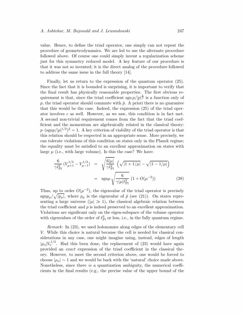
Finally, let us return to the expression of the quantum operator (25).Since the fact that it is bounded is surprising, it is important to verify thatthe final result has physically reasonable properties. The first obvious re-quirement is that, since the triad coefficient sgn p/|p| 12 is a function only ofp, the triad operator should commute with p. A priori there is no guaranteethat this would be the case. Indeed, the expression (25) of the triad oper-ator involves c as well. However, as we saw, this condition is in fact met.A second non-trivial requirement comes from the fact that the triad coef-ficient and the momentum are algebraically related in the classical theory:p ·(sgnp/|p|1/2)2 = 1. A key criterion of viability of the triad operator is thatthis relation should be respected in an appropriate sense. More precisely, wecan tolerate violations of this condition on states only in the Planck regime;the equality must be satisfied to an excellent approximation on states withlarge µ (i.e., with large volume). Is this the case? We have:

6

γℓ2Pl

(V1/3µ+1 − V

1/3µ−1) =

√

6|µ|γℓ2Pl

(

√

|1 + 1/µ| −√

|1 − 1/µ|)

= sgnµ

√

6

γ|µ|ℓ2Pl

(1 +O(µ−2)) (28)

Thus, up to order O(µ−2), the eigenvalue of the triad operator is preciselysgnpµ/

√

|pµ|, where pµ is the eigenvalue of p (see (21)). On states repre-senting a large universe (|µ| ≫ 1), the classical algebraic relation betweenthe triad coefficient and p is indeed preserved to an excellent approximation.Violations are significant only on the eigen-subspace of the volume operatorwith eigenvalues of the order of ℓ3Pl or less, i.e., in the fully quantum regime.

Remark : In (23), we used holonomies along edges of the elementary cellV. While this choice is natural because the cell is needed for classical con-siderations in any case, one might imagine using, instead, edges of length

|µo|V 1/3o . Had this been done, the replacement of (23) would have again

provided an exact expression of the triad coefficient in the classical the-ory. However, to meet the second criterion above, one would be forced tochoose |µo| ∼ 1 and we would be back with the ‘natural’ choice made above.Nonetheless, since there is a quantization ambiguity, the numerical coeffi-cients in the final results (e.g., the precise value of the upper bound of the


triad operator spectrum) should not be attached direct physical significance.In particular, for lessons for the full theory, one should use only the qualita-tive features and orders of magnitudes. The numerical values can be arrivedat only through a systematic reduction of the full quantum theory, wherethe precise value of |µo|(∼ 1) should emerge, e.g., as the lowest eigenvalue ofan appropriate geometric operator. We will return to this issue in the nextsection.

4 Quantum dynamics: The Hamiltonian constraint

Since the curvature is bounded above on the entire kinematical Hilbert spaceHS

grav, one might expect that the classical singularity at the big bang wouldbe naturally resolved in the quantum theory. In this section we will showthat this is indeed the case.

4.1 The quantum Hamiltonian constraint

In section 1, we reduced the Hamiltonian constraint to (11). However, wecan not use this form of the constraint directly because it is cast in termsof the connection c itself rather than holonomies. One can ‘regulate’ it interms of holonomies and then pass to quantum theory. However, to bringout the close similarity of the regularization procedure with the one followedin the full theory [14], we will obtain the same expression starting from theexpression of the classical constraint in the full theory:

Cgrav :=

∫

V

d3xN e−1(

ǫijkFiabE

ajEbk − 2(1 + γ2)Ki[aK

jb]E

ai E

bj

)

= −γ−2

∫

V

d3xN ǫijkFiab e

−1EajEbk (29)

where e :=√

|detE| sgn(detE). We restricted the integral to our cell V(of volume Vo with respect to oqab) and, in the second step, exploited thefact that for spatially flat, homogeneous models the two terms in the fullconstraint are proportional to each other (one can also treat both terms asin the full theory without significant changes [25]). Because of homogeneity,we can assume that the lapse N is constant and, for definiteness, from nowonwards we will set it to one.

As a first step in constructing a Hamiltonian constraint operator we haveto express the curvature components F i

ab in terms of holonomies. We will usethe procedure followed in the full theory [14] (or in lattice gauge theories).


Consider a square αij in the i-j plane spanned by two of the triad vectorsoeai , each of whose sides has length µoV

1/3o with respect to the fiducial metric

oqab.8 Then, ‘the ab component’ of the curvature is given by

F iabτi = oωi

aoωj

b

(

h(µo)αij − 1

µ2oV

2/3o

+O(c3µo)

)

(30)

The holonomy h(µo)αij in turn can be expressed as

h(µo)αij

= h(µo)i h

(µo)j (h

(µo)i )−1(h

(µo)j )−1 (31)

where, as before, holonomies along individual edges are given by

h(µo)i := cos

µoc

2+ 2 sin

µoc

2τi (32)

Next, let us consider the triad term ǫijk e−1EajEbk in the expression of

the Hamiltonian constraint. Since the triad is allowed to become degenerate,there is a potential problem with the factor e−1. In the reduced model, evanishes only when the triad itself vanishes and hence the required termǫijk e

−1EajEbk can be expressed as a non-singular function of p and thefiducial triads. In the full theory, the situation is more complicated andsuch a direct approach is not available. There is nonetheless a procedure tohandle this apparently singular function [14]: one expresses it as a Poissonbracket between holonomies and the volume function as in section 3.3 andthen promotes the resulting expression to an operator. To gain insight into this strategy, here we will follow the same procedure. Thus, let us beginwith the identity on the symmetry reduced phase space ΓS

grav:

ǫijkτi e−1EajEbk = −2(8πγGµoV

1/3o )−1 ǫabc oωk

c h(µo)k h(µo)

k−1, V (33)

where h(µ0)k is the holonomy along the edge parallel to the kth basis vector

of length µoV1/3o with respect to oqab. Note that, unlike the expression (30)

for F iab, (33) is exact, i.e. does not depend on the choice of µo.

Collecting terms, we can now express the gravitational part of the con-straint as:

Cgrav = −4(8πγ3µ3oG)−1

∑

ijk

ǫijktr(h(µo)i h

(µo)j h

(µo)−1i h

(µo)−1j h

(µo)k h(µo)−1

k , V )

+O(c3µo) (34)8In a model with non-zero intrinsic curvature, those edges would not form a closed

loop. The issue of how to deal with intrinsic curvature is discussed in [27].


where, the term proportional to identity in the leading contribution toF i

ab in (30) drops out because of the trace operation and where we used

ǫabc oωiaoωj

boωk

c =√

oq ǫijk. Note that, in contrast to the situation with triadsin section 3.3, now the dependence on µo does not drop out. However, one

can take the limit µo → 0. Using the explicit form of the holonomies h(µo)i ,

one can verify that the leading term in (34) has a well-defined limit whichequals precisely the classical constraint. Thus, now µo —or the length of theedge used while expressing Fab in terms of the holonomy around the squareαij— plays the role of a regulator. Because of the presence of the curvatureterm, there is no natural way to express the constraint exactly in terms ofour elementary variables; a limiting procedure is essential. This faithfullymirrors the situation in the full theory: there, again, the curvature term isrecovered by introducing small loops at vertices of graphs and the classicalexpression of the constraint is recovered only in the limit in which the loopshrinks to zero.

Let us focus on the leading term in (34). As in the full theory, this termis manifestly finite and can be promoted to a quantum operator directly.The resulting regulated constraint is:

C(µo)grav = 4i(γ3µ3

oℓ2Pl)

−1∑

ijk

ǫijktr(h(µo)i h

(µo)j h

(µo)−1i h

(µo)−1j h

(µo)k [h

(µo)−1k , V ])

= 96i(γ3µ3oℓ

2Pl)

−1 sin2 µoc

2cos2

µoc

2(35)

×(

sinµoc

2V cos

µoc

2− cos

µoc

2V sin

µoc

2

)

Its action on the eigenstates of p is

C(µo)grav |µ〉 = 3(γ3µ3

oℓ2Pl)

−1(Vµ+µo −Vµ−µo)(|µ+4µo〉−2|µ〉+ |µ−4µo〉) . (36)

On physical states, this action must equal that of the matter Hamiltonian−8πGCmatter.

Now, the limit µo → 0 of the classical expression (34) exists and equalsthe classical Hamiltonian constraint which, however, contains c2 (see (11)).

Consequently, the naive limit of the operator C(µo)grav also contains c2. How-

ever, since c2 is not well-defined on HSgrav, now the limit as µo → 0 fails

to exist. Thus, we can not remove the regulator in the quantum theory ofthe reduced model. In the full theory, by contrast, one can remove the reg-ulator and obtain a well-defined action on diffeomorphism invariant states[14]. This difference can be directly traced back to the assumption of homo-geneity.9 In the full theory, there is nonetheless a quantization ambiguity

9In the full theory, one triangulates the manifold with tetrahedra of coordinate volume


associated with the choice of the j label used on the new edges introduced todefine the operator corresponding to Fab [29]. That is, in the full theory, thequantization procedure involves a pair of labels (e, j) where e is a continuouslabel denoting the new edge and j is a discrete label denoting the spin onthat edge. Diffeomorphism invariance ensures that the quantum constraintis insensitive to the choice of e but the dependence on j remains as a quan-tization ambiguity. In the reduced model, diffeomorphism invariance is lostand the pair (e, j) of the full theory collapses into a single continuous label µo

denoting the length of the edge introduced to define Fab. The dependence onµo persists —there is again a quantization ambiguity but it is now labelledby a continuous label µo. Thus, comparison of the situation with that in

the full theory suggests that we should not regard C(µo)grav as an approximate

quantum constraint; it is more appropriate to think of the µo-dependence in(35) as a quantization ambiguity in the exact quantum constraint. This isthe viewpoint adopted in loop quantum cosmology.

If one works in the strict confines of the reduced model, there does notappear to exist a natural way of removing this ambiguity. In the full theory,on the other hand, one can fix the ambiguity by assigning the lowest non-trivial j value, j = 1/2, to each extra loop introduced to determine theoperator analog of Fab. This procedure can be motivated by the followingheuristics. In the classical theory, we could use a loop enclosing an arbitrarilysmall area in the a-b plane to determine Fab locally. In quantum geometry, onthe other hand, the area operator (of an open surface) has a lowest eigenvalueao = (

√3γ)/4 ℓ2Pl [17, 30] suggesting that it is physically inappropriate to

try to localize Fab on arbitrarily small surfaces. The best one could do is toconsider a loop spanning an area ao, consider the holonomy around the loopto determine the integral of Fab on a surface of area ao, and then extract aneffective, local Fab by setting the integral equal to aoFab. It appears naturalto use the same physical considerations to remove the quantization ambiguityalso in the reduced model. Then, we are led to set the area of the smallestsquare spanned by αij to ao, i.e. to set (γµo) ℓ

2Pl = ao, or µo =

√3/4. Thus,

while in the reduced model itself, area eigenvalues can assume arbitrarilysmall values, if we ‘import’ from the full theory the value of the smallest

µ3

o and writes the integral C(N) :=∫

d3xN ǫijkF iab e−1EajEbk as the limit of a Riemann

sum, C(N) = limµo→0

∑

µ3

oNǫijkF iab e−1EajEbk, where the sum is over tetrahedra. If

we now replace F by a holonomy around a square α of length µo, F ∼ µ−2

o (hα − 1),and the triad term by a Poisson bracket, e−1EE ∼ µ−1

o hh−1, V , and pass to quantumoperators, we obtain C(N) ∼ lim

∑

trhαh[h−1, V ]. The µo factors cancel out but, in thesum, the number of terms goes to infinity as µo → 0. However, the action of the operatoron a state based on any graph is non-trivial only at the vertices of the graph whenceonly a finite number of terms in the sum survive and these have a well defined limit ondiffeomorphism invariant states. In the reduced model, because of homogeneity, all termsin the sum contribute equally and hence the sum diverges.


non-zero area eigenvalue, we are naturally led to set µo =√

3/4. We will doso.

To summarize, in loop quantum cosmology, we adopt the viewpoint that(35), with µo =

√3/4, is the ‘fundamental’ Hamiltonian constraint operator

which ‘correctly’ incorporates the underlying discreteness of quantum geom-etry and the classical expression (11) is an approximation which is valid onlyin regimes where this discreteness can be ignored and the continuum pictureis valid. We will justify this assertion in section 4.3.

4.2 Physical states

Let us now solve the quantum constraint and obtain physical states. For sim-plicity, we assume that the matter is only minimally coupled to gravity (i.e.,there are no curvature couplings). As in general non-trivially constrainedsystems, one expects that the physical states would fail to be normalizablein the kinematical Hilbert space HS = HS

grav ⊗ HSmatter (see, e.g., [31, 18]).

However, as in the full theory, they do have a natural ‘home’. We again havea triplet

CylS ⊂ HS ⊂ Cyl⋆S

of spaces and physical states will belong to Cyl⋆S , the algebraic dual of CylS .Since elements of Cyl⋆S need not be normalizable, we will denote them by(Ψ|. (The usual, normalizable bras will be denoted by 〈Ψ|.)

It is convenient to exploit the existence of a triad representation. Then,every element (Ψ| of Cyl⋆S can be expanded as

(Ψ| =∑

µ

ψ(φ, µ)〈µ| (37)

where φ denotes the matter field and 〈µ| are the (normalized) eigenbras ofp. Note that the sum is over a continuous variable µ whence (Ψ| need notbe normalizable. Now, the constraint equation

(Ψ|(

C(µo)grav + 8πGC

(µo)matter

)†

= 0 (38)

turns into the equation

(Vµ+5µo − Vµ+3µo)ψ(φ, µ + 4µo) − 2(Vµ+µo − Vµ−µo)ψ(φ, µ) (39)

+ (Vµ−3µo − Vµ−5µo)ψ(φ, µ − 4µo) = −1

38πGγ3µ3

oℓ2Pl C

(µo)matter(µ)ψ(φ, µ)

for the coefficients ψ(φ, µ), where C(µo)matter(µ) only acts on the matter fields

(and depends on µ via metric components in the matter Hamiltonian). Note


that, even though µ is a continuous variable, the quantum constraint is adifference equation rather than a differential equation. Strictly, (39) justconstrains the coefficients ψ(φ, µ) to ensure that (Ψ| is a physical state.However, since each 〈µ| is an eigenbra of the volume operator, it tells us howthe matter wave function is correlated with volume, i.e., geometry. Now, ifone wishes, one can regard p as providing a heuristic ‘notion of time’, andthen think of (39) as an evolution equation for the quantum state of matterwith respect to this time. (Note that p goes from −∞ to ∞, negativevalues corresponding to triads which are oppositely oriented to the fiducialone. The classical big-bang corresponds to p = 0.) While this heuristicinterpretation often provides physical intuition for (39) and its consequences,it is not essential for what follows; one can forego this interpretation entirelyand regard (39) only as a constraint equation.

What is the fate of the classical singularity? At the big bang, the scalefactor goes to zero. Hence it corresponds to the state |µ = 0〉 in HS

grav. So,the key question is whether the quantum ‘evolution’ breaks down at µ = 0.Now, the discrete ‘evolution equation’ (39) is essentially the same as thatconsidered in the first papers on isotropic loop quantum cosmology [2, 3]and that discussion implies that the quantum physics does not stop at thebig-bang.

For completeness, we now recall the main argument. The basic idea is toexplore the key consequences of the difference equation (39) which determinewhat happens at the initial singularity. Starting at µ = −4Nµo for somelarge positive N , and fixing ψ(φ,−4Nµo) and ψ(φ, (−4N+4)µo), one can usethe equation to determine the coefficients ψ(φ, (−4N + 4n)µ0) for all n > 1,provided the coefficient of the highest order term in (39) continues to remainnon-zero. Now, it is easy to verify that the coefficient vanishes if and only ifn = N . Thus, the coefficient ψ(φ, µ=0) remains undetermined. In its place,we just obtain a consistency condition constraining the coefficients ψ(φ, µ=−4) and ψ(φ, µ = −8). Now, since ψ(φ, µ = 0) remains undetermined, atfirst sight, it may appear that we can not ‘evolve’ past the singularity, i.e.that the quantum evolution also breaks down at the big-bang. However,the main point is that this is not the case. For, the coefficient ψ(φ, µ =0) just decouples from the rest. This comes about because, as a detailedexamination shows, the minimally coupled matter Hamiltonians annihilateψ(φ, µ) for µ = 0 [1, 25] and Vµo = V−µo . Thus, unlike in the classical theory,evolution does not stop at the singularity; the difference equation (39) lets us‘evolve’ right through it. In this analysis, we started at µ = −4Nµo becausewe wanted to test what happens if one encounters the singularity ‘head on’.If one begins at a generic µ, the ‘discrete evolution’ determined by (39) just‘jumps’ over the classical singularity without encountering any subtleties.


To summarize, two factors were key to the resolution of the big bangsingularity: i) as a direct consequence of quantum geometry, the Hamiltonianconstraint is now a difference equation rather than a differential equationas in geometrodynamics; and ii) the coefficients in the difference equationare such that one can evolve unambiguously ‘through’ the singularity eventhough the coefficient ψ(φ, µ = 0) is undetermined. Both these features arerobust: they are insensitive to factor ordering ambiguities and persist inmore complicated cosmological models [6, 7].

Next, let us consider the space of solutions. An examination of theclassical degrees of freedom suggests that the freedom in physical quantumstates should correspond to two functions just of matter fields φ. The spaceof solutions to the Hamiltonian constraint, on the other hand is much larger:there are as many solutions as there are functions ψ(φ, µ) on an interval[µ′ − 4µo, µ

′ + 4µo), where µ′ is any fixed number. This suggests that alarge number of these solutions may be redundant. Indeed, to complete thequantization procedure, one needs to introduce an appropriate inner producton the space of solutions to the Hamiltonian constraint. The physical Hilbertspace is then spanned by just those solutions to the quantum constraintwhich have finite norm. In simple examples one generally finds that, whilethe space of solutions to all constraints can be very large, the requirementof finiteness of norm suffices to produce a Hilbert space of the physicallyexpected size.

For the reduced system considered here, we have a quantum mechanicalsystem with a single constraint in quantum cosmology. Hence it should bepossible to extract physical states using the group averaging technique ofthe ‘refined algebraic quantization framework’ [31, 18, 32]. However, thisanalysis is yet to be carried out explicitly and therefore we do not yet havea good control on how large the physical Hilbert space really is. This issueis being investigated.

The Hamiltonian constraint equation differs markedly from the Wheeler-DeWitt equation of geometrodynamics in the Planck regime because it cru-cially exploits the discreteness underlying quantum geometry. But one mightexpect that in the continuum limit µo → 0 —which, from the quantum ge-ometry perspective, is physically fictitious but nonetheless mathematicallyinteresting— the present quantum constraint equation would reduce to theWheeler-DeWitt equation. We will conclude this sub-section by showingthat this expectation is indeed correct in a precise sense.

To facilitate this comparison, it is convenient to introduce some notation.


Let us set

p =1

6γµℓ2Pl .

Then, the Wheeler-DeWitt equation can be written as

Cwdwgrav ψ(φ, p) :=

2

3ℓ4Pl [

√

|p|ψ(φ, p) ]′′ = 8πG Cmatter(p)ψ(φ, p) , (40)

where the prime denotes derivative with respect to p. If we now further set

ψ(p) :=1

6p−1

o (V6(p+po)/γℓ2Pl

− V6(p−po)/γℓ2Pl

)ψ(p) ,

with po = γℓ2Plµo/6, our quantum constraint (39) reduces to:

ˆC(µo)

grav ψ(φ, p) := − 1

12ℓ4Plp

−2o (ψ(φ, p + 4po) − 2ψ(φ, p) + ψ(φ, p − 4po))

= 8πGCmatter(p)ψ(φ, p) . (41)

From now on we will consider only those ‘wave functions’ ψ(φ, p) which aresmooth (more precisely, C4) in their p dependence. Then, it follows that

Cwdwgrav ψ(φ, p) = ˆC

(µo)

grav ψ(φ, p) + ℓ4PlO(p2o) ψ

′′′′(φ, p) (42)

+ ℓ4PlO(p2

o

p2) ψ′′(φ, p) + ℓ4PlO(

p2o

p3)ψ′(φ, p) + ℓ4PlO(

p2o

p4)ψ(φ, p)

Hence, in the limit po → 0 (i.e., µo → 0), we have

ˆC(µo)

grav ψ(φ, p) 7→ Cwdwgrav ψ(φ, p) (43)

whence the discrete equation (41) reduces precisely to the Wheeler-DeWittequation (40). Put differently, it has turned out that (41) is a well-defineddiscretization of (40).

One can also ask a related but distinct question: Is there a sense inwhich solutions to the Wheeler-DeWitt equation are approximate solutionsto the ‘fundamental’ discrete evolution equation? The answer is again in theaffirmative. Let us restrict ourselves to the part of the p-line where p≫ po,i.e., where the quantum volume of the universe is very large compared to thePlanck scale. Consider the restriction, to this region, of a smooth solutionψ(φ, p) to (40) and assume that it is slowly varying at the Planck scale inthe sense that ψ/ψ′ ∼ s, ψ/ψ′′ ∼ s2, etc, with po ≪ s ≤ p. Then, ψ(φ, p)is an approximate solution to the ‘fundamental’ quantum constraint (41) inthe sense that:

[

1 +O(p2

o

s2) +O(

p2o

p2) +O(

p2os

p3) +O(

p2os

2

p4)

]

ˆC(µo)grav ψ(φ, p) (44)

= 8πGCmatter(p)ψ(φ, p) .


Note that, in contrast to the discussion about the relation between the twoequations, we can not take the limit po → 0 because we are now interested inthe discrete evolution. The solution to the Wheeler-DeWitt equation is anapproximate solution to the fundamental equation only to the extent thatterms of the order O(p2

o/s2), O(p2

o/p2), O(p2

os/p3), O(p2

os2/p4) are negligi-

ble.

We will conclude with three remarks.

1) We saw in section 4.1 that the µo → 0 limit of the quantum constraint

operator C(µo)grav does not exist on HS

grav. Yet, in the above discussion ofthe ‘continuum limit’, we were able to take this limit. The resolution ofthis apparent paradox is that the limit is taken on a certain sub-space ofCyl⋆, consisting of smooth functions of p and none of these states belongto HS

grav. Indeed, since elements of HSgrav have to be normalizable with

respect to the inner product (17), they can have support only on a countablenumber of points; they cannot even be continuous. In particular, solutionsto the Wheeler-DeWitt equation can not lie in HS; they belong only to theenlargement Cyl⋆ of HS .

2) There is a close mathematical similarity between quantum cosmologydiscussed here and the ‘polymer particle’ example discussed in [22]. In thatexample, following the loop quantum gravity program, a new representa-tion of the Weyl algebra is introduced for a point particle in non-relativisticquantum mechanics. In this representation, the Weyl operators are unitarilyimplemented but weak continuity, assumed in the Von Neumann uniquenesstheorem, is violated for one of the two 1-parameter unitary groups. As aresult (although the position operator exists) the momentum operator —thegenerator of infinitesimal space translations— fails to exist. This is meantto reflect the underlying discreteness of geometry. The ‘fundamental’ quan-tum evolution is given by a difference equation. But there is a precise sensein which the standard Schrodinger evolution is recovered in the regime ofvalidity of non-relativistic quantum mechanics. The ‘fundamental’ discreteevolution is analogous to the present ‘fundamental’ quantum constraint (41)while the Schrodinger equation is the analog of the Wheeler-DeWitt equa-tion (40). Therefore, details of the polymer particle analysis provide goodintuition for the ‘mechanism’ that allows loop quantum cosmology to be verydifferent from the standard one in the Planck regime and yet agree with itwhen the universe is large compared to the Planck scale.

3) As mentioned in section 1, in this paper we do not address the difficultissue of systematically deriving quantum cosmology from full loop quantumgravity. Indeed, since CylS 6⊂ Cyl, at first it seems it would be difficult to


relate the two theories. However, note that the physical states of the sym-metry reduced model are elements of Cyl⋆S while those of the full theory areelements of Cyl⋆, and Cyl⋆S is contained in Cyl⋆: elements of Cyl⋆S are thosedistributions on the full quantum configuration space A which are supportedonly on the subspace AS of symmetric connections [33]. In particular, solu-tions to the quantum constraint discussed in this section do belong to Cyl⋆.Therefore, it should be possible to recover such states by first consideringthe full quantum theory and then carrying out a symmetry reduction.

4.3 Classical limit

In section 4.1, we found that the gravitational part of the Hamiltonian con-straint could not be introduced by a straightforward ‘quantization’ of theclassical constraint (11) because there is no direct operator analog of c onHS

grav. We then followed the strategy adopted in the full theory to arrive at

the expression (35) of C(µo)grav . To ensure that this is a viable quantization,

we need to show that (35) does reduce to (11) in the classical limit. In thissub-section, we will carry out this task.

For this purpose we will use coherent states peaked at points (co,Nµo)of the classical phase space where N ≫ 1 (i.e. the volume of the universeis very large compared to the Planck volume) and co ≪ 1 (late times, when

the extrinsic curvature is small compared to the fiducial scale V−1/3o ). At

such large volumes and late times, one would expect quantum correctionsto become negligible. The question then is whether the expectation value

of the quantum constraint C(µo)grav in these coherent states equals the classical

constraint (11) modulo negligible corrections. If so, C(µo)grav would have the

correct classical limit.

To construct a coherent state, we also have to specify the width d of theGaussian (i.e., ‘tolerance’ for quantum fluctuations of p). Now, since thequantum fluctuations in the volume of the universe must be much smallerthan the volume itself, d ≪ Nµo and since we also want the uncertainty inc to be small, we must have µo ≪ d. A coherent state of the desired type isthen given by:

|Ψ〉 =∑

n

[

exp (−((n −N)2µ2

o

2d2) exp (−i((n −N)µo)

co2

)

]

|nµo〉 (45)

(More precisely, |Ψ〉 is the ‘shadow’ on the regular lattice µ = nµo of thecoherent state in Cyl⋆ uniquely selected by the triplet (co,Nµo, d). For


details, see [22], Section 4.) Our task is to compute the expectation value

〈C(µo)grav〉 =

〈Ψ|C(µo)grav |Ψ〉

〈Ψ|Ψ〉 (46)

of the constraint operator (41):

C(µo)grav |µ〉 = 3(γ3µ3

oℓ2Pl)

−1(Vµ+µo − Vµ−µo) (|µ+ 4µo〉 − 2|µ〉 + |µ− 4µo〉) .

Let us first calculate the expectation value. Setting ǫ := µo/d, we have:

〈Ψ|C|Ψ〉 =∑

n,n′

exp(−1

2ǫ2((n′ −N)2 + (n−N)2))ei

co2

(n′−n)µo 〈n′µo|C|nµo〉

= 3(γ3µ3oℓ

2Pl)

−1∑

n,n′

exp(−1

2ǫ2((n′ −N)2 + (n−N)2))ei

co2

(n′−n)µo

×(V(n+1)µo− V(n−1)µo

) 〈n′µo|(|(n + 4)µo〉 − 2|nµo〉 + |(n − 4)µo〉)

= 3(γ3µ3oℓ

2Pl)

−1[

e2icoµo∑

n

exp(−1

2ǫ2((n + 4 −N)2 + (n−N)2))


)

−2∑

n

exp(−ǫ2(n−N)2) (V(n+1)µo− V(n−1)µo

)

+e−2icoµo

∑

n

exp(−1

2ǫ2((n − 4 −N)2 + (n−N)2))


)]

.

To simplify this expression further, we note that all three sums in this ex-pression are of the same form and focus on the first:

∑

n

exp(−1

2ǫ2((n + 4 −N)2 + (n−N)2)) (V(n+1)µo

− V(n−1)µo)

= e−4ǫ2∑

n

e−ǫ2(n−N)2 (V(n−1)µo− V(n−3)µo

)

where we have completed the square in the exponential and shifted the sum-mation index by 2. To compute this sum, as in [22], we use the Poissonresummation formula

∑

n

e−ǫ2(n−N)2f(n) =∑

n

∫

e−ǫ2(y−N)2f(y) e2πiyn dy . (47)


This integral can be evaluated using the steepest descent approximation (seeAppendix). One obtains:

∑

n

e−ǫ2(n−N)2 f(n) =

√π

ǫ

∑

n

f(N +iπn

ǫ2) e−

π2n2

ǫ2+2πinN (1 +O((Nǫ)−2))

=

√π

ǫf(N)(1 +O(e−π2/ǫ2) +O((Nǫ)−2)) (48)

where, in the last step, we used the fact that, since ǫ≪ 1, terms with n 6= 0are suppressed by the exponential. (Note that Nǫ ≫ 1 because Nµo ≫ d,i.e., the permissible quantum fluctuation in the volume of the universe ismuch smaller than the volume of the universe at the phase space pointunder consideration.)

Finally, we can collect terms to compute the expectation value (46).Using 〈Ψ|Ψ〉 = (

√π/ǫ)(1 +O(e−π2/ǫ2)), we have

〈C〉S = 3(γ3µ3oℓ

2Pl)

−1[

e−4ǫ2e2icoµo(V(N−1)µo− V(N−3)µo

)

−2(V(N+1)µo− V(N−1)µo

) + e−4ǫ2e−2icoµo(V(N+3)µo− V(N+1)µo

)]

×(1 + O(e−π2/ǫ2) +O((Nǫ)−2))

=1

2(γ2µ2

o)−1√

γµoℓ2Pl/6

[

e−4ǫ2e2icoµo((N − 1)3

2 − (N − 3)3

2 )

− 2((N + 1)3

2 − (N − 1)3

2 ) + e−4ǫ2e−2icoµo((N + 3)3

2 − (N + 1)3

2 )]

×(1 +O(e−π2/ǫ2) +O((Nǫ)−2))

=3

2(γ2µ2

o)−1√

γµoℓ2PlN/6 (e−4ǫ2e2icoµo − 2 + e−4ǫ2e−2icoµo)

×(1 +O(e−π2/ǫ2) +O((Nǫ)−2) +O(N−1))

= −6γ−2c2o√P (1 +O((Nǫ)−2) +O(N−1) +O(ǫ2) +O(c2o)) (49)

where we have set P := 16γµoℓ

2PlN and used the fact that co ≪ 1 and µo ∼ 1

(we also dropped corrections of order e−π2/ǫ2 since they are always dwarfedby those of order ǫ2). Thus, the expectation value equals the classical con-straint (11) up to small corrections of order c2o, ℓ

4Pl/(Pǫ)

2, ℓ2Pl/P and ǫ2.(Note that each of them can dominate the other corrections depending onthe values of the different parameters.) Hence, (35) is a viable quantizationof the classical expression (11).


5 Discussion

Let us begin with a brief summary of the main results. In section 2, we car-ried out a systematic symmetry reduction of the phase space of full generalrelativity in the connection variables. In the spatially flat model consideredhere, our connection coefficient c equals the only non-trivial (i.e. dynam-ical) component of the extrinsic curvature (modulo a factor of γ) and ourconjugate momentum p equals the only non-trivial metric component (mod-ulo sgn p). Hence, our symmetry reduced Hamiltonian description is thesame as that of geometrodynamics. By contrast, we saw in section 3 thatquantum theories are dramatically different already at the kinematic level.In loop quantum cosmology, the Hilbert space HS

grav is spanned by almostperiod functions of c while in geometrodynamics it would be spanned bysquare-integrable functions of c. The intersection between the two Hilbertspaces is only the zero element! In loop quantum cosmology, the fundamen-

tal operators are p and Nµ = exp(iµc/2); unlike in geometrodynamics, thereis no operator corresponding to c itself. Although p is unbounded and itsspectrum consists of the entire real line, all its eigenvectors are normaliz-able and the Hilbert space is the direct sum of the 1-dimensional sub-spacesspanned by the eigenspaces. In geometrodynamics, on the other hand, noneof the eigenvectors of p is normalizable; the Hilbert space is a direct inte-gral of its ‘eigenspaces’. This marked difference is responsible for the factthat, while the triad operator (which encodes the inverse of the scale factor)is unbounded in geometrodynamics, it is bounded in loop quantum cosmol-ogy. Consequently, in the state corresponding to the classical singularity,the curvature is large, but it does not diverge in loop quantum cosmology.

In section 4 we discussed the Hamiltonian constraint, i.e., quantum dy-namics. Because there is no direct operator analog of c, we had to introduce

the constraint operator C(µo)grav by an indirect construction. Here, we fol-

lowed the strategy used in the full theory [14], expressing curvature F iab of

the gravitational connection Aia in terms of its holonomies around suitable

loops. In the full theory, one can take the limit as the loop shrinks to zeroand obtain a well-defined operator on diffeomorphism invariant states. Thereduced model, by contrast, fails to be diffeomorphism invariant and theoperator diverges on HS

grav in the limit. Therefore, to obtain a well-definedoperator, we used loops enclosing an area ao, the smallest non-zero quan-tum of area in quantum geometry. The resulting operator can be regardedas a ‘good’ quantization of the classical constraint function because it hasthe correct classical limit. The resulting quantum constraint equation hasnovel and physically appealing properties. First, it is a difference –ratherthan differential— equation and thus provides a ‘discrete time evolution’.


Second, the coefficients in this difference equation are such that the ‘evo-lution’ does not break down at the singularity; quantum physics does notstop at the big-bang! This occurs without fine tuning matter or making itviolate energy conditions. Furthermore, while in consistent discrete modelsthe singularity is often ‘avoided’ because discrete ‘time steps’ are such thatone simply leaps over the point where the singularity is expected to occur[36], here, one can and does confront the singularity head on only to findthat it has been resolved by the quantum ‘evolution’. Furthermore, thesefeatures are robust [6, 7]. However, near the big-bang, the state is ‘extremelyquantum mechanical,’ with large fluctuations. Thus, the classical space-time‘dissolves’ near the big-bang. In this regime, we can analyze the structureonly in quantum mechanical terms; we can no longer use our classical in-tuition which is deeply rooted in space-times and small fluctuations aroundthem.

In the Planck regime, the predictions of loop quantum cosmology arethus markedly different from those of standard quantum cosmology basedon geometrodynamics. The origin of this difference can be traced back to thefact that while loop quantum cosmology makes a crucial use of the funda-mental discreteness of quantum geometry, standard cosmology is based on acontinuum picture. One would therefore expect that the difference betweenthe two would become negligible in regimes in which the continuum pictureis a good approximation. We established two results to show that this expec-tation is indeed correct. First, there is a precise sense in which the differenceequation of loop quantum cosmology reduces to the Wheeler-DeWitt differ-ential equation in the continuum limit. Second, in the regime far removedfrom the Planck scale, solutions to the Wheeler-DeWitt equation solve thedifference equation to an excellent accuracy. Thus, the quantum constraintof loop quantum cosmology modifies the Wheeler-DeWitt equation in a sub-tle manner: the modification is significant only in the Planck regime and yetmanages to be ‘just right’ to provide a natural resolution of the big-bangsingularity.

Next, let us re-examine the early papers on loop quantum cosmology interms of the precise mathematical framework developed in this paper. Inthe present terminology, in the previous discussion one effectively restrictedoneself just to periodic functions exp(inc/2), rather than almost periodicfunctions exp(iµc/2) considered here. Thus the gravitational Hilbert spaceHS,P

grav considered there is the rather small, periodic sub-space of the presentHS

grav. While this restriction did have heuristic motivation, it amounted toforcing c to be periodic.10 From the geometrodynamical perspective, the

10In the symmetry reduction, one began with the general geometric theory of invariantconnections and found that components of a homogeneous connection transform as scalars


extrinsic curvature was made periodic (with a very large period) and it wasthen not surprising that the eigenvalues of the scale factor (and hence alsothe volume) operator could only be discrete. However, a careful analysisshows that the restriction to periodic functions can not be justified: periodicfunctions fail to separate the symmetric connections. Thus, in the earliertreatments, the space of configuration variables was ‘too small’ already atthe classical level and this led to an artificial reduction in the size of thequantum state space.

In the analysis presented here, c is not periodic. As a consequence, thespectrum of the volume operator is the entire real line. Yet, there is dis-creteness in a more subtle sense: all eigenvectors of the volume operator arenormalizable. This is a direct consequence of the fundamental premise ofloop quantum gravity that the quantum Hilbert space carries well definedoperators corresponding to holonomies and not connections themselves. Inthe full theory, this feature does make the spectra of geometric operatorsdiscrete and their eigenvectors normalizable. Because of the homogeneityassumption, however, the first of these features is lost in loop quantum cos-mology but the second does survive. The surprising and highly non-trivialfact is that this is sufficient for several of the main results of earlier papersto continue to hold: i) the inverse scale factor is still bounded from above;ii) the Hamiltonian constraint is again a difference equation; and, iii) thecoefficients in this equation are such that the singularity is resolved in thequantum theory. Furthermore, the current analysis provided a systematic

approach to verify that the constraint operator C(µo)grav has the correct classi-

cal limit and made its relation to the Wheeler-DeWitt operator more preciseand transparent. However, as in earlier papers, the issue of finding the in-ner product on physical states is yet to be analyzed in detail. While thegroup averaging procedure [31, 18, 32] provides a natural avenue, a detailedimplementation of this program has only begun. The issue of whether the‘pre-classicality’ condition selects unique quantum states, thereby providinga natural solution to the issue of initial conditions can be addressed system-atically only after one has a better control on the physical Hilbert space.Finally, the discussion of section 4.3 not only shows that the classical Ein-stein’s equation is recovered in loop quantum cosmology in an appropriatelimit but it also provides a systematic approach to the problem of findingquantum corrections to Einstein’s equations.11 These corrections are now

under gauge transformations [34]. The appropriate, polymer theory for real-valued scalarfields was developed only recently [35] and requires, as in the present paper, the Bohrcompactification of the real line.

11There appears to be a rather general impression that Einstein’s equations are notmodified in loop quantum gravity. As our discussion of 4.3 shows, this is not the case. It istrue that we simply promoted the classical Hamiltonian constraint function to an operator.


being worked out systematically.

We conclude with a general observation. The way in which the big-bang singularity is resolved has potentially deep implications on questionsabout the origin of the universe. For instance, the question of whether theuniverse had a beginning at a finite time is now ‘transcended’. At first,the answer seems to be ‘no’ in the sense that the quantum evolution doesnot stop at the big bang. However, since space-time geometry ‘dissolves’near the big-bang, there is no longer a notion of time, or of ‘before’ or‘after’ in the familiar sense. Therefore, strictly, the question is no longermeaningful. The paradigm has changed and meaningful questions must nowbe phrased differently, without using notions tied to classical space-times.A similar shift of paradigm occurred already with the advent of generalrelativity. Before Einstein, philosophers argued that the universe could nothave a finite beginning because, if it did, one could ask what there wasbefore. However, this question pre-supposes that space-time is an eternal,passive arena and matter simply evolves in it. With general relativity, welearned that space and time are ‘born with matter’, whence the question of‘what was there before’ is no longer meaningful. Loop quantum cosmologybrings about a further shift of paradigm, weeding out certain questions thatseemed meaningful in classical general relativity and requiring that they bereplaced by more refined questions, formulated in the context of quantumspace-times.

Acknowledgments: We thank the participants in the ‘Quantum fieldtheory on curved space-times’ workshop at the Erwin Schrodinger Institutefor stimulating discussions. We are especially grateful to Bill Unruh forraising several conceptual issues addressed here, and to Klaus Fredenhagenfor the key observation that the Bohr compactification of the real line isthe appropriate quantum configuration space. This work was supported inpart by the NSF grant PHY-0090091, KBN grant 2P03B 2724, the Eberlyresearch funds of Penn State and the Erwin Schrodinger Institute.

However, because there is no direct operator analog of c, this ‘quantization’ is subtle andeven on semi-classical (coherent) states, sharply peaked at classical configurations, theexpectation value of the constraint operator equals the classical constraint function withsmall but very specific quantum corrections. We expect that the same procedure can beapplied in the full theory to obtain quantum corrections to full Einstein’s equations.


A Method of Steepest Descent

In this appendix, we will show that the method of steepest descent can beused to evaluate the right side of the Poisson resummation formula (47):

∑

n

e−ǫ2(n−N)2f(n) =∑

n

∫

e−ǫ2(y−N)2f(y) e2πiyn dy .

To begin with, we will assume that f is analytic and return to the cases ofinterest at the end.

Note first that the Fourier integral can be written as

∫

e−ǫ2(y−N)2f(y) e2πiyndy = N

∫

g(z) eNhn(z) dz ,

where g(z) = f(Nz) is the combination of volume eigenvalues, and

hn(z) := −ǫ2N(z − 1)2 + 2πinz .

For large N , the integral can be evaluated by the method of steepest descent.For this, we have to first find the saddle points. In our case, this amounts tofinding solutions z0 of h′(z0) = −2ǫ2N(z0−1)+2πin = 0. This equation hasa single solution, z0 = 1 + iπn/Nǫ2. Steepest paths through z0 are definedby constant imaginary part Imhn(z) = Imhn(z0). If we write z = ξ+ iη withreal ξ, η, we obtain −2ǫ2N(ξ − 1)η + 2πnξ = 2πn, which has the solutionsξ = 1 or η = πn/ǫ2N . We can now deform the original integration alongthe real line to an integration along the steepest path η = πn/ǫ2N , i.e.z = t+ iπn/ǫ2N with t real. Next, let us change the integration variable tou by t = 1 + u/ǫ

√N such that

u2 = hn(z0) − hn(z) = ǫ2N(t− 1)2 .

With dz = du/ǫ√N we obtain

∫

g(z) eNhn(z) dz = ǫ−1N− 1

2

∫ ∞

−∞

g(t(u) + iπn/ǫ2N) eN(hn(z0)−u2) du .

So far, everything was exact. In order to be able to compute the integral,we now use the Taylor expansion:

g(t(u) + iπn/ǫ2N) = g(1 + u/ǫ√N + iπn/ǫ2N) = g(1 + iπn/ǫ2N)

+ug′(1 + iπn/ǫ2N)/ǫ√N + u2g′′(1 + iπn/ǫ2N)/ǫ2N

+O(u3/ǫ3N3

2 )


Then, the integral can be evaluated approximately as [37]:

∫

g(z) eNhn(z) dz = ǫ−1N− 1

2

[

g(1 + iπn/ǫ2N)

∫ ∞

−∞

eN(hn(z0)−u2)du

+ǫ−2N−1g′′(1 + iπn/ǫ2N)

∫ ∞

−∞

u2eN(hn(z0)−u2)du

+ O(ǫ−4N−2

∫ ∞

−∞

u4eN(hn(z0)−u2)du)

]

=√πǫ−1N−1g(1 + iπn/ǫ2N)e−π2n2/ǫ2+2πinN

×(1 +O((Nǫ)−2)) ,

where the corrections of order (Nǫ)−2 are small because d ≪ Nµo. (Weassumed g′′(z0) to be of the same order as g(z0), which is the case for thefunctions we are interested in here.)

We can now return to the Poisson re-summation formula and computethe sum:

∑

n

e−ǫ2(n−N)2f(n) =∑

n

∫

e−ǫ2(y−N)2f(y) e2πiyn dy

= N∑

n

∫

f(Nz) eNhn(z) dz

=√πǫ−1

∑

n

f(N + iπn/ǫ2) e−π2n2/ǫ2+2πinN

×(1 +O((Nǫ)−2))

=√πǫ−1f(N)(1 +O(e−π2/ǫ2) +O((Nǫ)−2))

where, in the last step, we used the fact that terms with n 6= 0 are suppressedby the exponential because ǫ≪ 1.

Finally, let us address the fact that the functions f(y) of interest in themain text come from the eigenvalues of the volume operator which are of thetype Vnµo = (γ|n|µo/6)

3/2 and, because of the absolute value involved, f(y)fail to be analytic in y at y = 0. One can circumvent this potential problemby replacing them with functions f(y) which are the analytic continuations(to the upper half complex y-plane) of the restriction of f(y) to the positivereal y-axis and then carry out the above calculation for f which, by construc-tion, are analytic. (Thus, for example, |y|3/2 is replaced by (y2)3/4.) Theerror,

∑

n exp(−ǫ2(n −N)2) [f(n) − f(n)], can be shown to be of the order

O(e−(Nǫ)2) which is negligible compared to the corrections derived above.The error is so small because the function integrated on the right side ofthe Poisson resummation formula is strongly peaked at a very large positive


value y = N of y and the contribution from the negative half of the real yaxis is extremely small.

References

[1] M. Bojowald, Inverse scale factor in isotropic quantum geometry, Phys.Rev., D64 (2001), 084018.

[2] M. Bojowald, Loop quantum cosmology IV: Discrete time evolutionClass. Quant. Grav., 18 (2001), 1071–1088.

[3] M. Bojowald, Absence of singularity in loop quantum cosmology, Phys.Rev. Lett., 86 (2001), 5227–5230.

[4] M. Bojowald, Dynamical initial conditions in quantum cosmology, Phys.Rev. Lett., 87 (2001), 121301.

[5] M. Bojowald, Inflation from quantum geometry, Phys. Rev. Lett., 89

(2002), 261301.

[6] M. Bojowald, Quantization ambiguities in isotropic quantum geometry,Class. Quantum Grav., 19 (2002), 5113–5130.

[7] M. Bojowald, Homogeneous loop quantum cosmology, Class. QuantumGrav., 20 (2003), 2595–2615.

[8] A. Ashtekar and C. J. Isham, Representation of the holonomy algebras ofgravity and non-Abelian gauge theories, Class. Quant. Grav., 9 (1992),1433–1467.

[9] A. Ashtekar and J. Lewandowski, Representation theory of analyticholonomy algebras, in ‘Knots and Quantum Gravity’, edired by J.C.Baez, Oxford U. Press, Oxford 1994.

[10] J.C. Baez, J.C. Generalized measures in gauge theory, Lett. Math.Phys., 31 (1994), 213-223.

[11] D. Marolf and J. Mourao, On the support of the Ashtekar-Lewandowskimeasure, Commun. Math. Phys., 170 (1995), 583-606.

[12] A. Ashtekar and J. Lewandowski, Projective techniques and functionalintegration, Jour. Math. Phys., 36 (1995), 2170-2191.

[13] A. Ashtekar and J. Lewandowski, Differential geometry on the space ofconnections using projective techniques, Jour. Geo. & Phys., 17 (1995),191–230.


[14] Thiemann, T. (1996) Anomaly-free formulation of non-perturbative,four-dimensional Lorentzian quantum gravity, Phys. Lett., B380

(1996), 257–264;Quantum spin dynamics (QSD), Class. Quant. Grav., 15 (1998), 839–873;QSD V : Quantum gravity as the natural regulator of matter quantumfield theories, Class. Quant. Grav., 15 (1998), 1281–1314.

[15] A. Ashtekar and J. Lewandowski,Background independent quantumgravity: A status report (pre-print, 2003)

[16] A. Ashtekar, New variables for classical and quantum gravity, Phys.Rev. Lett., 57 (1986), 2244–2247;New Hamiltonian formulation of general relativity, Phys. Rev., D36

(1987), 1587–1602.

[17] A. Ashtekar and J. Lewandowski, Quantum theory of geometry I: Areaoperators, Class. Quant. Grav., 14 (1997), A55–A81.

[18] A. Ashtekar, J. Lewandowski, D. Marolf, J. Mourao, and T. Thiemann,Quantization of diffeomorphism invariant theories of connections withlocal degrees of freedom, Jour. Math. Phys., 36 (1995), 6456–6493.

[19] H. Sahlmann, H. Some comments on the representation theory of thealgebra underlying loop quantum gravity, gr-qc/0207111.

[20] J. Lewandowski and A. Okolow, Diffeomorphism covariant representa-tions of the holonomy-flux star-algebra, gr-qc/0302059.

[21] H. Sahlmann and T. Thiemann, On the superselection theory of theWeyl algebra for diffeomorphism invariant quantum gauge theories,gr-qc/0302090.

[22] A. Ashtekar, S. Fairhurst and J. Willis, Quantum gravity, shadow states,and quantum mechanics, Class. Quantum Grav., 20 (2003), 1031-1062.

[23] C. Rovelli and L. Smolin, Spin networks and quantum gravity, Phys.Rev., D52 (1995), 5743–5759.

[24] J. C. Baez, Spin networks in non-perturbative quantum gravity, in ‘TheInterface of Knots and Physics’, edited by Kauffman, L. (AmericanMathematical Society, Providence, 1996) pp. 167–203;Spin networks in gauge theory, Adv. Math. 117 (1996), 253–272.

[25] M. Bojowald, Isotropic loop quantum cosmology, Class. Quantum Grav.,19 (2002), 2717–2741.


[26] A. Ashtekar, J. Baez, A. Corichi and K. Krasnov, Quantum geometryand black hole entropy, Phys. Rev. Lett., 80 (1998), 904–907.A. Ashtekar, J. Baez and K. Krasnov, Quantum geometry of isolatedhorizons and black hole entropy, Adv. Theo. Math. Phys., 4 (2000),1–95.

[27] M. Bojowald, G. Date and K. Vandersloot, Homogeneous loop quantumcosmology: The role of the spin connection, (in preparation).

[28] M. Bojowald, The semiclassical limit of loop quantum cosmology, Class.Quantum Grav., 18 (2002), L109–L116.

[29] M. Gaul and C. Rovelli, A generalized Hamiltonian constraint operatorin loop quantum gravity and its simplest Euclidean Matrix Elements,Class. Quantum Grav., 18 (2001), 1593–1624.

[30] C. Rovelli and L. Smolin, Discreteness of area and volume in quantumgravity, Nucl. Phys. B442 (1995), 593–622; Erratum: Nucl. Phys. B456

(1995) 753S. Frittelli, L. Lehner and C. Rovelli, The complete spectrum of the areafrom recoupling theory in loop quantum gravity, Class. Quant. Grav. 13

(1996), 2921–2932

[31] Marolf, D. Refined algebraic quantization: Systems with a single con-straint, gr-qc/9508015.

[32] T. Thiemann, QSD III: Quantum constraint algebra and physical scalarproduct in quantum general relativity, Class. Quantum Grav. 15 (1998),1207–1247.

[33] M. Bojowald, and H. A. Kastrup, Symmetry reduction for quantized dif-feomorphism invariant theories of connections, Class. Quantum Grav.,17 (2000), 3009–3043.

[34] M. Bojowald, Loop quantum cosmology: I. Kinematics, Class. QuantumGrav., 17 (2001), 1489–1508.

[35] A. Ashtekar, J. Lewandowski and H. Sahlmann, Polymer and Fock rep-resentations for a Scalar field, Class. Quantum Grav. 20 (2003), L1–11.

[36] R. Gambini and J. Pullin, Discrete quantum gravity: applications tocosmology, gr-qc/0112033.

[37] A. Erdelyi, Asymptotic expansions, Chapter II (Dover, New York, 1956).

Mathematical structure of loop quantum cosmology

Documents