Commun. Math. Phys. 174, 561-604 (1996) Communications IΠ Mathematical Physics © Springer-Verlag 1996 Combinatorial Quantization of the Hamiltonian Chern-Simons Theory II Anton Yu. Alekseev 1 ' *, Harald Grosse 2 ' **, Volker Schomerus 3 ' *** 1 Institute of Theoretical Physics, Uppsala University, Box 803 S-75108, Uppsala, Sweden 2 Institut fur Theoretische Physik, Universitat Wien, Austria 3 Harvard University, Department of Physics, Cambridge, MA 02138, USA Received: 9 September 1994/in revised form: 31 January 1995 Abstract: This paper further develops the combinatorial approach to quantization of the Hamiltonian Chern Simons theory advertised in [1]. Using the theory of quan- tum Wilson lines, we show how the Verlinde algebra appears within the context of quantum group gauge theory. This allows to discuss flatness of quantum con- nections so that we can give a mathematically rigorous definition of the algebra of observables stfcs of the Chern Simons model. It is a *-algebra of "functions on the quantum moduli space of flat connections" and comes equipped with a positive functional ω ("integration"). We prove that this data does not depend on the par- ticular choices which have been made in the construction. Following ideas of Fock and Rosly [2], the algebra s/cs provides a deformation quantization of the algebra of functions on the moduli space along the natural Poisson bracket induced by the Chern Simons action. We evaluate a volume of the quantized moduli space and prove that it coincides with the Verlinde number. This answer is also interpreted as a partition partition function of the lattice Yang-Mills theory corresponding to a quantum gauge group. 1. Introduction This paper is a second part of the series devoted to combinatorial quantization of the Hamiltonian Chern Simons theory. Here we continue and essentially complete the analysis started in [1]. * On leave of absence from Steklov Mathematical Institute, Fontanka 27, St. Petersburg, Russia; e-mail: [email protected]. Supported by Swedish Natural Science Research Council (NFR) under the contract F-FU 06821- 304 and by the Federal Ministry of Science and Research, Austria. ** Part of project P8916-PHY of the 'Fonds zur Fόrderung der wissenschaftlichen Forschung in Osterreich'; e-mail: [email protected]. *** Supported in part by DOE Grant No DE-FG02-88ER25065;e-mail: [email protected]. Present address: Institut fur Theoretische Physik, Universitat Hamburg, Luruper Chaussee 149, D-22761 Hamburg, Germany.

Welcome message from author
This document is posted to help you gain knowledge. Please leave a comment to let me know what you think about it! Share it to your friends and learn new things together.
Transcript
Commun. Math. Phys. 174, 561-604 (1996) Communications IΠ
MathematicalPhysics
© Springer-Verlag 1996
Combinatorial Quantization of the HamiltonianChern-Simons Theory II
Anton Yu. Alekseev1' *, Harald Grosse2' **, Volker Schomerus3' ***1 Institute of Theoretical Physics, Uppsala University, Box 803 S-75108, Uppsala, Sweden2 Institut fur Theoretische Physik, Universitat Wien, Austria3 Harvard University, Department of Physics, Cambridge, MA 02138, USA
Received: 9 September 1994/in revised form: 31 January 1995
Abstract: This paper further develops the combinatorial approach to quantization ofthe Hamiltonian Chern Simons theory advertised in [1]. Using the theory of quan-tum Wilson lines, we show how the Verlinde algebra appears within the contextof quantum group gauge theory. This allows to discuss flatness of quantum con-nections so that we can give a mathematically rigorous definition of the algebra ofobservables stfcs of the Chern Simons model. It is a *-algebra of "functions onthe quantum moduli space of flat connections" and comes equipped with a positivefunctional ω ("integration"). We prove that this data does not depend on the par-ticular choices which have been made in the construction. Following ideas of Fockand Rosly [2], the algebra s/cs provides a deformation quantization of the algebraof functions on the moduli space along the natural Poisson bracket induced by theChern Simons action. We evaluate a volume of the quantized moduli space andprove that it coincides with the Verlinde number. This answer is also interpretedas a partition partition function of the lattice Yang-Mills theory corresponding to aquantum gauge group.
1. Introduction
This paper is a second part of the series devoted to combinatorial quantization ofthe Hamiltonian Chern Simons theory. Here we continue and essentially completethe analysis started in [1].
* On leave of absence from Steklov Mathematical Institute, Fontanka 27, St. Petersburg, Russia;e-mail: [email protected] by Swedish Natural Science Research Council (NFR) under the contract F-FU 06821-304 and by the Federal Ministry of Science and Research, Austria.** Part of project P8916-PHY of the 'Fonds zur Fόrderung der wissenschaftlichen Forschung in
Osterreich'; e-mail: [email protected].*** Supported in part by DOE Grant No DE-FG02-88ER25065;e-mail: [email protected] address: Institut fur Theoretische Physik, Universitat Hamburg, Luruper Chaussee 149,D-22761 Hamburg, Germany.
562 A. Yu. Alekseev, H. Grosse, V. Schomerus
To set the stage let us reproduce the well-recognizable landscape of 3D ChernSimons theory. The latter is a 3-dimensional topological theory defined by the action
CS(A) = -^Tr/ (AάA + Λ . (1.1)4π M \ * J
Here M is a 3-dimensional manifold, A is a gauge field taking values in somesemi-simple Lie algebra and A: is a positive integer. In this setting the theory enjoysboth gauge and reparametrization symmetry which makes it topological. Elementaryobservables satisfying the same symmetry conditions may be constructed for eachclosed contour Γ in M as
(1.2)
Choosing the manifold M to be a product of a circle and a 2-dimensional orientablesurface Σ, one gets a Hamiltonian formulation of the model. The direction alongthe circle plays the role of time. Actually, one can relax topological requirementsand treat the problem locally. Then such a splitting into time and space directions isalways possible. The problem of quantization in the Hamiltonian approach may bestated as follows. One should construct quantum analogoues WΓ of the observables(1.2) corresponding to space-like contours. The main questions which arise in thisway are the following. We should describe the algebra generated by Wp in termsof commutation or exchange relations. Next, if we are going to use this algebraas a quantum algebra of observables, a *-operation and a positive inner productare necessary. The final step is to construct *-representations of the algebra ofobservables. Linear spaces which carry such representations may be used as Hubertspaces of the corresponding quantum systems.
The Hamiltonian formulation of the Chern Simons theory leads directly to themoduli space of flat connections on a Riemann surface. The latter appears as a phasespace of the Chern Simons model. The action (1.1) introduces a natural symplecticform and a Poisson bracket on the moduli space. So, one can look for quantizationof this moduli space in the framework of deformation quantization. This is actuallya mathematical reformulation of the same problem as Hamiltonian quantization ofthe Chern Simons model.
In the spirit of deformation quantization one should start with the Poisson bracketon the moduli space. This object was considered for some time in mathematicalliterature and there are several descriptions of the corresponding Poisson structure.The one suitable for our purposes has been suggested recently by Fock and Rosly[2]. The main idea of this approach is to replace a 2-dimensional surface by ahomotopically equivalent fat graph. This gives a finite-dimensional or combinatorialdescription of the moduli space. The name "combinatorial quantization" originatesfrom this fact. Another important achievement of [2] is that the only object whichis used in the description of the Poisson bracket is a classical r-matrix (solutionof the classical Yang-Baxter equation). When the Poisson bracket is represented interms of r-matrices, the quantization procedure is almost straightforward. Roughlyspeaking, one has to replace solutions of the classical Yang-Baxter equation by thecorresponding solutions of the quantum Yang-Baxter equation. In conclusion, theway to deformation quantization of the moduli space was much clarified by [2].
In [1] we have started a description of the quantum algebra of observables. Wehave introduced such an algebra for any pair of a fat graph and a semi-simple rib-bon quasi-Hopf algebra. There we followed the ideas of [2]. The novelties of our
Combinatorial Quantization of the Hamiltonian Chern-Simons Theory II 563
approach were introduction of the *-operation and of the quantum Haar measure onthe algebra of observables. A Haar measure on this type of algebras has been pre-viously considered in [3]. We succeeded to extend our consideration to quasi-Hopfalgebras as well. This is motivated by the fact that the most interesting examples- like quantum groups at roots of unity - do not meet the condition of semi-simplicity. After a certain truncation, however, they become semi-simple (weak)quasi-Hopf-algebras [4,5]. Thus, all the essential technical tools for quantization ofthe moduli space were introduced in [1]. On the other hand, an important piece ofthe quantization was still missing there: the quantum analogue of the flatness condi-tion. The "algebra of observables" stf eventually included some field configurationswith nonzero curvature. In this paper we overcome this problem and complete theprogram of quantization.
The quantized algebra of functions on the moduli space (moduli algebra) isexpected to provide the description of the algebra of observables in 3-dimensionalChern Simons theory. In principle, we can change the point of view at this pointand treat the theory of graph connections with a quantum gauge group as a sortof 2-dimensional lattice gauge theory. As usual, one may be interested in corre-lation functions of Wilson line observables provided by the trace functional. This2-dimensional interpretation has its own continuous counterpart. Assuming that in3-dimensional formulation the moduli algebra reproduces the algebra of observablesof the Chern Simons model exactly, one concludes that in the 2-dimensional for-mulation we obtain an exact lattice counterpart of gauged WZW model or so-calledG/G model (for the relation of CS and G/G model, see e.g. [6]). From time totime it is useful to switch from 3-dimensional interpretation to 2-dimensional andback. So, we shall use the vocabulary of both these approaches.
Let us give a short description of the content of each section. Section 2 collectsmain theorems of [1]. This gives the possibility to understand the results of the paperwithout referring to [1]. However, we do not give any proofs here and refer theinterested reader to the original text. Section 3 is devoted to Wilson line observablesWp. In particular, we prove that for Γ being a contractible contour, Wp belongs tothe center of the algebra of observables. We study in detail the commutative algebragenerated by Wr for a given Γ. It is proved to coincide with the celebrated Verlindealgebra. On the basis of the Verlinde algebra we construct central projectors inthe algebra stf and define a quantum analogue of the flatness conditions on thegraph. The algebra of observables s$cs with the condition of flatness imposed isour final answer for the quantized algebra of functions on the moduli space offlat connections. In Sect. 4 we prove the correctness of our definition. From thevery beginning we replace the surface by a fat graph. This can be done in manyways. We prove that observable algebras ^Cs which arise from different graphs arecanonically isomorphic to each other. We pick up a particular graph which consistsof a bunch of circles intersecting in only one point on the surface and describe thealgebra thereon in Sect. 4.2. Then we revisit the "multidimensional Haar measure"in Sect. 5.1, and obtain a graph independent "quantum integration" for jtfcs Thisis used in Sect. 5.2 to determine the volume of the quantum moduli space.
Let us mention here that there is an ambiguity in normalization of the "integra-tion measure." In this paper we use some particular normalization which may bereferred to as lattice Yang-Mills measure. The corresponding volume of the quantummoduli space resembles the answer for the partition function in the 2-dimensionalYang-Mills theory. Along with this normalization there exists a canonical one whichis fixed by the requirement that the volume of each simple ideal in the moduli
564 A. Yu. Alekseev, H. Grosse, V. Schomerus
algebra should be equal to the square root of its dimension. The volume of themoduli space evaluated by means of the canonical measure reproduces the famousVerlinde formula for the number of conformal blocks in the WZW model [7]. Inthis way we get a consistency check of our approach. In the 2-dimensional inter-pretation the Verlinde formula gives the answer for the partition function of ourlattice gauge model. It coincides with the experience of the continuous G/G model(see e.g. [8]). Advertising here this result, we postpone a more detailed discussionto the next paper.
For simplicity, we work with ribbon Hopf-algebras throughout most of the text.The generalization to ribbon quasi-Hopf algebras is explained in Sect. 6. Proofs forthis section are partly given in a separate appendix of the paper. Let us mentionthat there is a formal overlap between some of the results in Sects. 3,5 and therecent work of Buffenoir and Roche [15]. While their work is restricted to realdeformation parameters q, we are interested in the "physical" case where the defor-mation parameter is a root of unity. This causes a number of problems connectede.g. with *-structures and semisimplicity. Once they are overcome, the theory atroots of unity has the advantage of involving only finite sums and allowing for thebeforementioned physical application to Chern-Simons theories.
After this brief introduction we turn to a more systematic presentation of themain results. There are two basic ingredients used as the input for our construction.The first one is a semi-simple ribbon (weak quasi-) Hopf algebra . Equivalenceclasses of irreducible representations of <& are labeled by I,J,K, . . .. Furthermore oneneeds a compact orientable Riemann surface Σ&tm of genus g and with m punctures.These punctures are then marked so that the representation class 7V is assigned tothe vth point (v = l,...,m).
Our combinatorial approach requires to replace Σgtfn by a homotopically equiv-alent fat graph G and to equip G with some extra structure called "ciliation." Theciliated graph will be denoted Gcn. In [1] we assigned a *-algebra 3S(GC\\) to thisciliated graph. It is generated by quantum lattice connections and quantum gaugetransformations. A *-subalgebra j/(G) C &(GC\\) generated by invariant quantumlattice connections has to be singled out. Our attempt to implement the flatness con-dition that will finally lead to Chern-Simons observables, is based on the followingtheorem.
Theorem I (Fusion algebra and characteristic projectors). For every contractίbleplaquette P of the graph (or lattice) G, there is a set of central elements c!(P) Gjtf C $ which satisfy the fusion algebra (or "Verlinde algebra"), i.e.
cl(P)cJ(P) = YJNI
K
JcK(P), (1.3)K
(c!(P)T=c!(P). (1.4)
If the matrix S/j = Λf(\xl
q ® tr^)(R'R), J^ being equal to some nonzero real
number, is ίnvertίble, a set of characteristic projectors χ!(P) can be constructedfrom the elements c!(P). They are central orthogonal projectors within j/, i.e.
Explicit formulas for both cl(P) and χf(P) can be given (see Eqs. (3.19) and(3.22) below).
Combinatorial Quantization of the Hamiltonian Chern-Simons Theory II 565
Projectors are the analogue of characteristic functions on a manifold in the non-commutative framework. We will show that the "support" of χ°(P) consists of amanifold quantum connections, which have trivial monodromy around the plaquetteP. So χ°(P) plays the role of the δ-function at the group unit. A similar constructionhas been developed in [3]. This consideration motivates the following construction
of an algebra J^cs °f Chern-Simons observables,
**cs} = ** Π Λ^)Π/V(ΛO . (1.6)v=ι
Here Pv, v = 1, . . . , w, denotes the plaquette containing the vth puncture on Σ^m.It is marked by 7V. ^o is the set of all plaquettes on the graph G, which do notcontain a marked point.
Actually £#cs comes w^m some extra structure. First the *-operation on jtf
restricts to £#cs Moreover, the generalized "multidimensional Haar measure" ωon ,s/ which was constructed in [1] furnishes a positive linear functional ωcs on
jtfcs These data turn out to depend only on the input (Γίy?m,^).
Theorem II (Chern Simons observables). The triple ( ^ , *,ωCls) of an alge-
bra J&CS with ^-operation * and a positive linear functional ωcs ^ cs ^ does not depend on the choice of the fat ciliated group Gcι\ which is used in theconstruction.
Positive linear functional generalizes the concept of integration. Having con-structed ωcs will allow us to calculate the volume of the quantum moduli space.Actually, it coincides with the Verlinde number assigned to the same Riemann sur-face with marked points. This may be considered as a representative consistencycheck of the combinatorial approach.
2. Short Summary of [1]
Before we continue our study of Chern-Simons observables we want to review somenotations and results from [1]. We will not attempt to make this section selfcontainedbut keep our emphasis on formulas and notations frequently used throughout therest of this paper. Compared with [1], our notations will be slightly changed toadapt them to our new needs.
The theories to be considered here live on a graph (or lattice) G. The latterconsists of sites x,y,z e S and oriented links ±/,±/,±& G L. We also introduce amap t from the set of oriented links L to the set of sites S such that t(ί) = x, if ipoints towards the site x. Let us assume that two sites on the graph are connectedby at most one link (we will come back to this assumption later).
Our models on the graph G will possess a quantum gauge symmetry, which isdescribed by a family of ribbon Hopf *-algebras assigned to the sites x G S. Theyconsist of a *-algebra &x with co-unit εx, co-product AX9 antipode £fX9 R-matήx Rx
and the ribbon element vx. Let us stress that we deal with structures for which theco-product Ay. is consistent with the action
(ξ 0 η)* = η* 0 £* for all η,ξe&x
566 A. Yu. Alekseev, H. Grosse, V. Schomerus
of the *-operation * on elements in the tensor product <§x ® . This case is ofparticular interest, since it appears for the quantized universal enveloping algebrasUq(^) when the complex parameter q has values on the unit circle [5].
Given the standard expansion of Rx G &x ® &x, Rx = Σrxσ ® rxσ, one con-structs the elements
Among the properties of ux (cp. e.g. [9]) one finds that the product ux£fx(ux) is inthe center of &x. The ribbon element vx is a central square root of ux^x(ux) whichobeys the following relations:
v2
x = uxyx(ux), yx(vx) = vX9 εx(vx) = 1 , (2.2)
vx = υ~\ Δx(vx) = (R'xRxΓ\vx ® vx) . (2.3)
The elements ux and vx can be combined to furnish a grouplike element gx =u~lvx G $x. It will play an important role throughout the text. So let us list someproperties here:
(2.4)
Examples of ribbon-Hopf * -algebras are given by the quantized enveloping algebrasof all simple Lie algebras [9].
The algebras &x at different sites x are assumed to be twist equivalent, i.e. theHopf-structure of every pair of symmetry algebras ^x,^y is related by a (unitary)twist in the sense of DrinfePd [10]. We emphasize that - for the moment - werestrict ourselves to co-associative co-products Ax. As in [1], the discussion of thequasi-co-associative case is included at the end of the paper.
The total gauge symmetry is the ribbon Hopf-* -algebra & — (^)^X9 with theinduced co-unit ε, co-product A, etc. There is a canonic embedding of &x into ^and we will not distinguish in notations between the image of this embedding andthe algebra &X9 i.e. the symbol &x will also denote a subalgebra of &.
Representations of the algebra & of gauge transformations are obtained as fami-lies (τx)X£s of representations of the symmetries ^x. At this point let us assume that&x are semίsίmple and that every equivalence class [J] of irreducible representationsof &x contains a unitary representative τ^ with carrier space VJ . For the moment,the most interesting examples of gauge symmetries, e.g. Uq(^),qp = 1, are ruledout by this assumption. It was explained in Sect. 7 of [1] how "truncation" can curethis problem once the theory has been extended to quasi-Hopf algebras.
The tensor product τx \Eί τζ of two representations τ!
χ9 τζ of the semisimple al-gebra &x can be decomposed into irreducibles τx . This decomposition determinesthe Clebsch-Gordon maps Ca
x[IJ\K} \VI^VJ\-^ Vκ ',
Ca
x[IJ\K}(τ( El τί )(£) = τκ
x(ξ)Ca
x[IJ\K] . (2.6)
The same representations τx in general appears with some multiplicity N%J . Thesuperscript a — l9...9NχJ keeps track of these subrepresentations. It is common tocall the numbers Nj/ fusion rules. Normalization of these Clebsch Gordon mapsis connected with an extra assumption. Notice that the ribbon element vx is centralso that the evaluation with irreducible representations τx gives complex numbersv1 = τx(vx) (twist equivalence of the gauge symmetries implies that τ^(ι^) does not
Combinatorial Quantization of the Hamiltonian Chern-Simons Theory II 567
depend on the site x). We suppose that there exists a set of square roots κ/,κj — v1 ,such that
Ca
x[IJ\K](R'xyjCb
x[IJ\LΓ = <S«, A,L— . (2.7)
Here R'x = Σr2
xσ ® rxσ and (/ζ)/J = (τx ® X^X Let us analYze tm's relation inmore detail. As a consequence of intertwining properties of the Clebsch Gordonmaps and the /^-element, τκ(ξ) commutes with the left-hand side of the equation.So by Schurs' lemma, it is equal to the identity eκ times some complex fac-tor ωab(IJ\K). After appropriate normalization, ωab(IJ\K) — δa^ω(IJ\K) with acomplex phase ω(IJ\K). Next we exploit the *-operation and relation (2.3) to findωab(IJ\K)2 = v/vj /vκ. This means that (2.7) can be ensured up to a possible sign±. Here we assume that this sign is always +. This assumption was crucial forthe positivity in [1]. It is met by the quantized universal enveloping algebras of allsimple Lie algebras because they are obtained as a deformation of a Hopf-algebrawhich clearly satisfies (2.7).
We wish to combine the phases KJ into one element κx in the center of &X9 i.e.by definition, κx will denote a central element
κx E &x with τ^Ocjt) = KJ . (2.8)
Such an element does exist and is unique. It has the property K* — κ~{.The antipode £fx of furnishes a conjugation in the set of equivalence classes
of irreducible representations. We use [J] to denote the class conjugate to [J]. Someimportant properties of the fusion rules Nj/ can be formulated with the help of thisconjugation. Among them are the relations
N£* = 1, N*K
J = N^1 = Nf* . (2.9)
The numbers v1 are symmetric under conjugation, i.e. vκ = vκ . Let us also mentionthat the trace of the element ^x(ux)v~λ in a given representation τ7 computes the"quantum dimension" dj of the representation τ1 [9], i.e.
rfjΞtΓίτV)). (2.10)
The numbers dj satisfy the equalities didj — ΣNχJdκ and dκ = dg.We can use the Clebsch Gordon maps C[KK\0] to define a "deformed trace"
tή. If^GEnd(F^), then
. (2.11)
This definition simplifies with the help of the following lemma which will be appliedfrequently within the next section.
Lemma 1. The Clebsch-Gordon maps C[KK\$\ satisfy the following equations:
1. For all ξ G &x they obey the intertwining relations,
id) - Cx[KK\0](id ® τf (&x(ξ))) ,
id)Cx[KK\θγ - (id 0 τϊ(&x(ξ)))Cx[KK\0]* . (2.12)
568 A. Yu. Alekseev, H. Grosse, V. Schomerus
2. With normalization conventions (2.7) one finds
dκ**(Cx[KK\0]*Cx[KK\0\) = eκ ,
= eκ . (2.13)
Here action of the trace \xκ on the first resp. second component is understoodand eκ = e% is the identity map on Vκ.
Proof. The first two relations are a consequence of the intertwining properties ofC[^£|0] and the defining relations of an antipode £fx. Using (2.12) one can checkthat the traces on the left-hand side of Eqs. (2.13) commute with τκ(ξ) and henceare proportional to the identity e% . To calculate the normalization, one multiplieswith τκ(g), evaluates the tr* of the expression and uses the normalization (2.7) ofthe Clebsch Gordon maps.
As a consequence of this lemma we find the simple formula
x)). (2.14)
In particular this implies that d& — ir^(eκ).
While the gauge transformations ξ G & live in the sites of G, variables U!
ab(i) areassigned to the links of the graph G. They can be regarded as "functions" on thenon-commutative space of lattice connections. Together with the quantum gaugetransformations ξ £ ^ they generate the lattice algebra 36 defined in [1]. To writethe relations in J*, one has to introduce some extra structure on the graph G. Theorientation of the Riemann surface Σ determines a canonical cyclic order in theset Lx = {i G L : t(i) — x} of links incident to the vertex x. Writing the relations in$ we were forced to specify a linear order within Lx. To this end one considersciliated graphs Gcn. A ciliated graph can be represented by picturing the underlyinggraph together with a small cilium cx at each vertex. For i,j G Lx we write i ^ y,if (cx,i,j) appear in a clockwise order.
In contrast to [1], we will write relations in 3% in a matrix notation. This meansthat the generators U!
ab(I) G Si are combined into one single object
Such algebra valued matrices are widely used in similar contexts and will havemany advantages for the calculations to be done later. With this remark we areprepared to review the defining relations of £8. The rest of our notations will beexplained as we proceed.
^ is characterized by three different types of relations.
1. Covariance properties of the generators Ul
ab(i) under gauge transforma-tions are the only relations involving the generators ξ G . If jc = t(i), y = t(—i),they read
ξU'(i) = U'(i)ι4(ξ) for all ξε9x,
μfy(ξ)U'(i) = U'(l)ξ for all ξeyy,
ξUl(i) = U'(i)ξ for all ξ € &2, z £ {x,y} . (2.15)
Combinatorial Quantization of the Hamiltonian Chern-Simons Theory II 569
Here we used the symbol μx(ξ) G End(F7) (8) $ which is defined by
μ[(ξ) = (τ(® i ά ) A z ( ξ ) for a l l i e d . (2.16)
The covariance relations (2.15) make sense as relations in End(F7)(g)^, if ξ isregarded as an element ξ G End( V1 ) 0 $ with trivial entry in the first component.We will not distinguish in notation between elements ξ G & and their image in
2. Functorίalίty for elements U!(i) on a fixed link / confirms again that U\i)is a covariant object with respect to two copies of the Hopf algebra acting fromthe left and from the right,
U!(i)UJ(i) = ^Ca
y[IJ\KTUK(i)Ca
x[IJ\K] , (2.17)ΛΓ,α
ul(i)ul(-i) = 4, υ\-ϊ)υl(ί) = 4 . (2.18)The Clebsch Gordon maps C;[IJ\K]9 Ca
y[IJ\Kγ have been introduced in the lastsection. One can view their appearance in the multiplication rule as a consequenceof the generalized (for Hopf algebras) Wigner-Eckhart theorem. It is important thatthe left and right indices of U!(i) always belong to conjugate representations. Inthis respect the subalgebra formed by the matrix elements of U f ( i ) resembles analgebra of functions on the quantum group1. To explain the small numbers on top ofthe U9 one has to expand U*(i) G End(F7) 0 3t according to U*(i) = Σ w7 (g> u!
σ.Then
U1 = mI
σ^eJ ®u!
σ
and similarly for UJ (ί). Here and in the following, ej denotes the identity mapon VJ.
3. Braid relations between elements C/7(z), UJ(j) assigned to different linkshave to respect the gauge symmetry and locality of the model. These principlesrequire
U!(i)UJ(j) = UJ(j)U!(i) for all ij e L without common endpoints , (2.19)
U I ( i ) U J ( j ) = UJ(j)UI(i)RI
x
J for all ij G L with t(i) =x = t(j) and i <j.(2.20)
R[J is the matrix ((τ7 0 τ^)(^) 0 e) e End(F7) <g> End(FJ) 0 OS.
Braid relations for other configurations of the links ij can be derived. As anexample we consider a case where j, —i point towards the same site x and —i> j.Then
UJ(j)(RjJU'(i) - U'(i)U\j) . (2.21)
In this form, braid relations will be widely used throughout the text.Let us briefly describe some of the results obtained in [1]. The lattice algebra J*
allows for a ^-operation. Its definition uses the elements κx introduced in (2.8), or
1 More precisely, there exist symmetry valued matrices F!
x G End( V1) 0 x such that theU!(i)Fx's generate a subalgebra of ^ which is isomorphic to the dual of the symmetry Hopf-
algebra #„. (see also [1]).
570 A. Yu. Alekseev, H. Grosse, V. Schomerus
rather the element K G <& they determine in <& = Π^ Before we can explain how* acts on , we need some more notations. Let σκ : : & ι— > be the automoφhismof J* obtained by conjugation with the unitary element K G , i.e.
K^Ffc for all F G J* .
σκ extends to an automoφhism of End(F)®^ with trivial action on End(F).Suppose furthermore that BeEnd(V)®& has been expanded in the formB = mσ ®Bσ with mσ 6 End(K) and Bσ e J*. If V is a Hubert space and m* theusual adjoint of the linear map mσ, the *-operation on induces a *-operation onEnd(K) 0 ^ by means of the standard formula ^* = m* 05*. With these nota-tions, the definition for * in [1] becomes
(£/'(i))* = σ^Xc-zXtf;1)7) (2 22)Again / is supposed to point from y = t(—i) towards x — t(i) and R[ = (τ[ 0id)(#z)EEnd(F7)<S>^, etc.
Another ingredient in the theory of the lattice algebra 3$ is the functional ω :$ H-> C. It can be regarded as the quantum analog of a multidimensional Haarmeasure. If we assume that the links z'v, v =!,...,«, are pairwise different, i.e. / V Φ± //t for all v φ μ, then
ω(t/7'(/ι) - - £/ / Λ(ιΛX) = 6(0^,0 5/Λ,o (2.23)
for all ξ G and every set of labels /v. Details and examples of explicit calculationswith ω can be found in [1].
It is interesting to consider the quantum analog of functions on the space oflattice connections. They form a subset (U) in $. More precisely, (U) is generatedby the matrix elements U!
ab(i} G & of quantum lattice connections U!(i) with thelabels /, / running through all their possible values. Here the word "generate" refersto the operations of addition and multiplication in , while the action of * is notincluded. So - except from special cases - (U) will not be a *-subalgebra of .This is one of the reasons, why we prefer to call (U) a subset (as opposed tosubalgebra) of . The other reason is related to the case of quasi-Hopf symmetries^ which will be discussed below. One of the main results in [1] is
Theorem 1 (Positivity) [1]. Suppose thai all the quantum dimensions dj are pos-itive and that relation (2.7) is satisfied. Then
ω(F*F) ^ 0 for all F G (£/}
and equality holds only for F = 0.
In this theorem, the argument F*F of the functional ω is in & rather than in(U). Since ω was defined on the whole lattice algebra ^ the evaluation of ω(F*F)is possible nevertheless.
Invariants within the subset (U) are the quantum analog of invariant functionson the space of lattice connections. They form a subset jtf,
*/ = {A G (U) C &\ξA = Aξ for all ξ G } .
Actually, stf C (U) is also a subalgebra of and the *-operation on & does restrictto a *-operation on stf . The positivity result of Theorem 1 implies that ω restricts
Combinatorial Quantization of the Hamiltonian Chern-Simons Theory II 571
to a positive linear functional on the *-algebra j/ (under the conditions of thetheorem). Let us finally mention that j/ is independent of the position of ciliawhich entered the theory when we defined 38.
3. The Quantum-Curvature and Chern Simons Observables
Observables of Chern-Simons theories are obtained from the algebra (U) C & of"functions" on the space of the quantum lattice connection in a two-step procedure.The restriction to invariants was described in [1]. The second step is to impose theflatness condition. This will be achieved in Sect. 3.2 below after some preparationin the first subsection.
3.1. Monodromy Around Plaquettes. To begin with let us consider a single pla-quette P on the graph G. We assume that all cilia at sites on the boundary dP ofthis plaquette lie outside of P. In more mathematical terms we can describe thisas follows: suppose that ij are two links on dP and that /(/) = x = t(j). Withoutany restriction we can take / ^ j. If k G L is a third link on G with t(k) = x and/ ^ k ^ y , then / = k or / = j, which means that in the situation encountered herethere can be no link in between ij.
Next let ^ be a curve on dP, i.e. a set of links {/v}v=ι,...,n with t(iv) =t(—iv+\), v = l , . . . , w — 1. Its inverse — # is the ordered set — = {— ΪΛ+I-V}V=I,...,Λ.On the set of curves ^ one can introduce a weight w(^) according to
n-\
= Σ sgn(/v, /v+i ), wherev=l
f - 1 if i < -j
Obviously, w(^) changes the sign, if the orientation of ^ is inverted, i.e.-w(-#).
From now on we will assume that ^ moves in a strictly counter-clockwisedirection on dP, i.e. — iv+\ > ίv for all v = l , . . . , / ι — 1. The starting point t(—C) =t(—i\ ) of # will be called y while we use x to denote the endpoint x = t(^) = t(in).
The quantum-holonomy along ^ is the family {t/7(0}/ of elements U!(i) Gdefined by
Here K/ are the complex numbers which have been postulated in relation (2.7). Letus gather some of the properties of the holonomies in the following proposition.
Proposition 2 (Properties of £/7(^)). If <& satisfies the requirements describedabove and ^ is not closed (i.e. t(^)ή=t(— )), the holonomies U1^) have thefollowing properties:
1. They commute with gauge transformations ξ G Xγ for all xv = t(iv\v = ! , . . . , « — 1. In other words, the holonomies are gauge invariant except fortheir endpoίnts.
572 A. Yu. Alekseev, H. Grosse, V. Schomerus
2. They commute with UJ(ί) if the endpoίnts of i and the endpoints of <& aredisjoint,
whenever {t(i\ t(-i)} Π {*(#), /(-#)} = 0.
3. They satisfy the following "functoriality on curves"
(3.2)
- 4 , (3.3)
an d behave under the action of * as
(U!(V)T = σ^lξU^-VKR-1)1) . (3.4)
4. The elements U1^) and £/7(-^) are related by
(3.5)
where g^ — (τ*(gy) ® eκ\
Proof. 1. is essentially trivial. 2. is an application of the braid relations for compositeelements (Proposition 6, [1]). If i has no endpoint on # the assertion is trivial. Let ussuppose that / has one endpoint z e S on %> and zφjt, j;. Without loss of generalitywe assume z = t(i). We decompose the curve ^ into two parts ] = λ , = 2
such that ^7l(^?2) ends (starts) at z. The corresponding elements (77(^v) satisfystandard braid relations with UJ(i\ i.e.
if ^l,-^2 < i. Similar relations with (R'z ') instead of Rz hold if C1,-^2 > ί.Because of the assumptions on #, other possibilities on the order of ^\-^2J donot exist. In the first case, braid relations for composite elements imply that
1 / ' / 2 2 J 2 J 1 / l /
1
Again, R has to be substituted by R' in case that ίίί1, —Ή2 > /. The representationτ° appears because C/7^1)^7^2) is invariant in z. Since (τ° ® τ/)(Λ z) = (εzΘτ/)C#z) = e/, we obtain the desired commutation relation. The last case in whichboth endpoints of / lie on the curve ^ is treated in a similar fashion.
3. We prove the first relation by induction on the length n of the curve (€. Forn — 1, <β = i\ and the relation holds because of functoriality on the link i\. So letus assume that the equation is correct for curves of length n — 1. We decompose ^into a curve & of length n — 1 and one additional link in. Using the definition of
the braid relations (2.21) and functoriality for curves of length less than n
Combinatorial Quantization of the Hamiltonian Chern-Simons Theory II 573
we obtain
jC^KL
Here z = t(%') and we used relation (2.7) for the last equality. The other twoformulas in 3. are obvious. 4. is a generalization of the formula (4.8) in [1] withinour new notations. We want to justify it here. It follows from the functoriality ofholonomies (3.2) and relation (2.7) that
Cy[KK\0](R'yfκU*(V) = vKCx[KK\0]UK(-%).
Here we also applied K&K£ — VK With the intertwining relation (2.12) of the Cleb-
sch Gordon maps C[^AΓ|0] and the definition of g^ = (τ^(gy) 0 e\ this can berewritten in the form
1 -s l K - 2 KC ϊΊSrKr\(\\πK.TT f(/?\ 11 Γ* \W\Γ\\ΊΊ ( (#\y[KK\()\gyU (Ή ) = VκLsX[KK \(J\U ( — 15 J .
Multiplication with CX[KK\Q]* and taking the trace iτκ results in the desired ex-pression for Uκ(—^) as a consequence of Eq. (2.13).
Let us now turn to the definition of monodromies. This corresponds to the caseof closed curves ^ which was excluded in the preceding proposition. ^ starts andends in the point x on dP. For such holonomies we introduce the new notation
M7(^) Ξ U!(^) for # closed . (3.6)
Proposition 3 (Properties of the monodromies). If ^ w a closed curve which satis-fies the requirements described above, the monodromies M7(^) have the followingproperties:
1. They commute with all gauge transformations ξ G ^ with ξ ^ &x. Theirtransformation behavior under elements ξ G &x is described by
2. They commute with UJ(i) if x is not among the endpoints of i, i.e. x^i),t(-i)}.3. They satisfy the following "functoriality on loops":
^) = Σ Ca
x[IJ\K]*MK(^)Ca
x[IJ\K] , (3.7)
e[ , (3.8)
574 A. Yu. Alekseev, H. Grosse, V. Schomerus
and behave under the action of * as
(Ml(^)Y = σΛ/ζXί-tfXO') (3 9)
4. The elements M7(^) and M7(-^) are related by
Mκ(-^) = dκt^(Cx[KK\QTCx[KK\Q]g^M^(^)RJκ). (3.10)
Proof. 1, 2. are obvious from the proof of Proposition 2. For the proof of 3.one breaks ^ into two non-closed parts ^\^2 such that t(^\) = y = ^(—^2) andexploits the simple braid relation
UI((ig2)RI
x
JUJ((igl) = UJ(<gl)(R'yyjUI(<#2) . (3.11)
Using the functoriality of the holonomies L/r/((^v) derived before, the functorialityon loops follows. Giving more details on the proof of 3, 4 would amount to arepetition of the proof of Proposition 2.
Remark. From the functoriality relations (3.7) of the monodromies one derives thefollowing quadratic relations:
M1 (^)R1/MJ(^)R^ = R(J MJ (%)RfI
χ
J M1 (%). (3.12)
Relations of this form were found to describe the quantum enveloping algebras ofsimple Lie algebras [11].
From the monodromies one can prepare new elements cl e stf C &. For theclosed curve ^ on the boundary dP of the plaquette P we define
cf = J(p) = Kl^q(M!(V)) = K/tΛM'Wτ^)). (3.13)
We recall that τx(gx) = gx = τx(u~lvx) and the last equality is a consequence ofLemma 1. The elements c1 have a number of beautiful properties. They will turnout to be central elements in the algebra j/ of invariants in (U) and satisfy thedefining relations of the fusion algebra.
Proposition 4 (Properties of c7). If all eyelashes at sites on the boundary of theplaquette P lie outside of P, the elements c1 = cl(P) have the following properties:
1. They are independent of the choice of the start- and endpoint x of the closedcurve C6.
2. They are central in the lattice algebra &. In particular c1 are invariantelements in (U) and hence central in j/.
3. They satisfy the fusion algebra
clcj = Y,NI
K
JcK , (3.14)K
=cr. (3.15)
Proof 1. We break the curve ^ at an arbitrary point y on dP and start again fromthe braid relations of the holonomies on the two pieces Ή*,^2 of ,
Ul(^λ)R^Ul(^2) - U'&WJ'U'W1). (3.16)
Combinatorial Quantization of the Hamiltonian Chern-Simons Theory II 575
y with g!
y from the right and with g[ from the leand me expansion R~} = Σs\σ ®s2
zσ result in
Now multiply with g!
y from the right and with g[ from the left. Usage of τI
x(ξ)gI
x =
yσJJ y\ yσJ^ \ '
• ~ ' '' <?')> . (3.17)
Here we made use of the formula («9£ 0 id )(/?;,) = Ry
l. We will insert this for-mula frequently in the following without further mention. After multiplying thetwo matrix components in the last equation we take the trace tr7. With u[ —
σK2
σ) = (v!)2τ'z(Slσ^-](s
2
zσ)) the result is
Finally, we insert g(u[ = υ1 , Definitions (3.6,2.11) of the monodromy M7(#) andthe g-trace tr^ to end up with
where <$' starts in the site y and runs along ^2 and <€\ to end up in y again. Thismeans that instead of x one can choose any other site y on the boundary of P todefine c1 .
2. is a simple consequence of the properties of the monodromy (Proposition 3)and 1.
3. The first relation is easily obtained from the "operator products" (3.7) of
the monodromy. One just multiplies the latter from the right with gxgx(R~ιyj
KjKj, uses the relation Ca
x\IJ \K\gfy = g^Cx[IJ\K] (this is (2.5)) and takes thetrace of both matrix-components of the equation. For the right-hand side of (3.7)this leads to
r.h.s. = ic/KΛtr7
K,a K
where we also inserted the normalization (2.7) of the Clebsch-Gordon maps andthe definition of the numbers N^J . The evaluation of the left-hand side is equally
simple. After application of the intertwining relation of g^ and the trace propertyfor tr7 one obtains
.
The simple calculation rxσ^~\rxτ) <g) r^τr%σ = ^~l(rxτs]
xσ) 0 ^τsxσ = e 0 e shows
l.h.s. - /c/KXtr7 ( g ) t r y [ M / ^ M J ^ = c1 cj .
576 A. Yu. Alekseev, H. Grosse, V. Schomerus
Let us turn to the behavior of c' under the action of *. The relation (3.9) impliesthat
= K^M^-Vrtte1)] = /cΓ'tr'tM't-^). (3.18)
Here sxσ are still defined by the expansion R~l = Σsxσ ®sxσ and we used therelations ux = έ%(sxσ)sxσv
2 and u~λ = sxσέ%(sxσ) (sum over σ is understood). Forthe fourth equality we inserted the quasi-triangularity of the element Rx. μ7(£) wasdefined in (2.16). It also appears in the transformation law of the monodromies
ξ) for all ξe&x.
The latter was used in the above calculation to shift the factor μx(slσ) from the leftto the right of M7(^). After this step, another application of the quasi-triangularityleads to the final result of the above calculation.
At this point we can insert the relation (3.10) and apply Lemma 1 several times:
(c7)* = K^d^tr1' 0lrO[CΛ[//|0]*CΛ[//|0]^M/(«')/^/Jί]
= c1
3.2. The Algebra stfcs of Chern Simons Observables. The results of the precedingsubsection show that for every plaquette P on the graph G there is a family {c!(P)}ιof elements in the center of j/(G) with the properties
c1(P)c\P) =
These elements are obtained as follows: suppose that j/(G) has been constructedwith some fixed ciliation on G. The corresponding ciliated graph will be denotedby GC,I. Now choose an arbitrary plaquette P and some ciliation on G such thatno cilium lies inside of P. We call this ciliated graph Gc i l/. By Proposition 12 inf l ] we know that there is an isomorphism E : j/(Gcil/) ι—> j3/(GCu). We can nowuse the expressions in the first subsection to construct the elements c1 explicitly inj/(Gcil/). Their images c!(P) =E(c!) in jtf(Gc\\) will be central and generate thefusion algebra. The automorphism E has been constructed in [1]. From the general
Combinatorial Quantization of the Hamiltonian Chern-Simons Theory II 577
action of E and the definition (3.13) for c1 one can obtain the explicit expression
c'(P) = (K/Γ^+Xίί/'α, )t/'(i2) . . . t/'(iπ)) > (3-19)
where {/Ί,/2, •••,*«} is a closed curve that surrounds P once and w(dP) = w({/ι,/2,
. . .,/„}) =b 1 if the cilium at c = φ'Λ) lies msίde the plaquette P. Formula (3.19) nolonger depends on the position of cilia.
Let us describe next, how one obtains "characteristic projectors" χ!(P) fromthe Casimirs cJ(P). In fact this step is quite standard, but it requires an additionalassumption on the gauge symmetries . From now on we suppose that the matrix
( \~}/2
with Jf = f £ 4 < oo (3.20)
is ίnvertible. A number of standard properties of S can be derived from the in-vertibility (and properties of the ribbon Hopf-* -algebra). We list them here withoutfurther discussion. Proofs can be found e.g. in [12].
= SJLSIL(^dLΓ] (3.21)K
with Cjj = NQJ . For the relations in the second line, the existence of an inverse ofS is obviously necessary. Invertibility of S is also among the defining features of amodular Hopf-algebra in [13].
Theorem 5 (Characteristic projectors). Suppose that the matrix S = (S/j) definedin Eq. (3.20) is invertible so that it has the properties stated in (3.21). Then theelements χJ(P) G stf defined by
χ'(P) = JΓd,(SC)lκcκ(P) = ^d,S1KcK(P) (3.22)
are central orthogonal projectors in s/, i.e. they satisfy the following relations:
χ'(Pγ = χ!(P), χ'(P)χJ(P) = δu χ!(P) . (3.23)
Proof. The simple calculation needs no further comments,
χ Y =
578 A. Yu. Alekseev, H. Grosse, V. Schomerus
Let us also determine the action of * on the projectors χ7,
(χ'γ = jrdlsΓj(cJγ = jvd,SjlC
J = χ' .
This concludes the proof of Theorem 5. The result is quite remarkable and centralfor our final step in constructing Chern Simons observables.
Consider once more the graph G that we have drawn on the punctured Riemannsurface Σ. Suppose that G has M plaquettes P, m of which contain a marked point.The latter will be denoted by Pv, v = 1 , . , . , / w . Let us use ^ for the set of allplaquettes on G and &Q for the subset of plaquettes which do not contain a markedpoint. By construction, the plaquettes Pv contain at most one puncture which ismarked by a label 7V. To every family of such labels 7V, v = l,. . . ,ra, we canassign a central orthogonal projector in j/.
m
)= Π ΛP)Π/V(Λ) (3.24)
Since all elements χ7(P) commute with each other, the order of multiplication isirrelevant.
Definition 6 (Chern Simons observables). The algebra £#£$ of Chern Simonsobservables on a Riemann surface Σ with m punctures marked by 7V, v = 1, . . . , w,is given through
(3.25)
Remark. Notice that the *-operation on j/ restricts to a *-operation on £/cs> Thesame is true for the positive linear functional in [1].
To call elements in stfcs "Chern Simons observables" has certain aspects ofa conjecture. A full justification of this name needs a detailed comparison withother approaches to quantized Chern-Simons theories. This is discussed at lengthin a forthcoming paper [14]. Some remarks are also made in the last section ofthis paper. At this point we can only give a more "physical" argument by showingthat elements in <$#cs have "their support on the space of lattice connections whichare flat everywhere except for the marked points." So whenever we multiply anelement A £ ^Cs with the matrix M7(^) and wraps around a plaquette P e &Q,only the contributions from flat connections survive in MJ(%>). Since flat connectionshave trivial monodromy, this means that for all A G £#csτ AMJ(^) ~ AeJ up to acomplex factor which depends on the conventions. This will follow from the nextproposition.
Proposition 7 (Flatness). The elements χ°(P) and M7(^) satisfy the followingrelation:
(3.26)
Here ^ is a closed curve on the boundary dP of the plaquette P which starts andends in the site x.
Proof. The point of departure is the operator product of the monodromies (Eq. (3.7)),
Combinatorial Quantization of the Hamiltonian Chern-Simons Theory II 579
As in the proof of Proposition 4.3 we obtain
= */ Σ ^Cx[ΪI\0](Rx
ιyjc;[IJ\K]*Mκ(V)
= */ Σ -Cx[KK\^(R'xy^Ca
x[JK\ϊγCa
x[JK\ϊ]
Mκ(V)(R'xfκCx[KK\0]* .
While the second equality follows from the definition (2.11) of the g-trace, the thirdequality is a consequence of the following lemma.
Lemma 2. The Clebsch-Gordon maps satisfy the following two relations:
Cx[ΪI\0](R'xyjCx[IJ\K]* =
a/vK
with an ίnvertible, complex matrix A.
The proof of the lemma relies on intertwining properties and normalizationsof Clebsch Gordon maps. Since it is somewhat similar to the proof of Lemma1- though certainly more sophisticated - we leave details to the reader.
As we continue to calculate χ°MJ(^), we will use the completeness of ClebschGordon maps, i.e. the relation
Σ -^—(R'xy^C;[JK\I]*Cx[JK\I] = ej 0 / . (3.27)la KJKK
With χ° = Σ ^dic1 it follows that
580 A. Yu. Alekseev, H. Grosse, V. Schomerus
4. Changing the Graph G
The quantum algebra <$#£$ is shown to depend only on the marked Riemannsurface Σ^m with punctures labeled by 7V and the quantum symmetry (S. Then aparticular graph is described which allows for a relatively simple presentation ofeβ/cs This presentation will be useful for explicit calculations (see e.g. Sect. 5.2)and the discussion of representation theory in a forthcoming paper [14].
4.1. Independence of the Graph. We plan to prove some fundamental isomorphismswithin this section. The algebra j/ of invariants can be constructed in many differentways. One first chooses a fat graph G on the punctured Riemann surface Σ^m andequips it with cilia at all the sites. Then one constructs the lattice algebra ^ for thisciliated graph and considers the algebra stf of invariants in (U) C 3$. Even though@& depends on the position of eyelashes, the algebra ^ that is obtained followingthese steps does not (Proposition 12, [1]). We will see now that the concrete choiceof the graph G is also irrelevant once we restrict ourselves to the subalgebra j/csof "functions" on the quantum moduli space of flat connections (as long as thegraph G is homotopically equivalent to the punctured Riemann surface ΣίΛ/M).
Proposition 8 (Dividing a link). Let G\ be a graph and construct a second graphG2 from G\ by choosing an arbitrary link ί on G\ and introducing an additionalsite x on ί so that i is divided into two links i\,i2 on G2 with t(i2) = t(ί\ t(—ί\) =t(-i) and t ( i \ ) = t(-i2) = x. Then the algebras stf\ = sf(G\) and 2 = <^(G2)are isomorphic as ^-algebras.
Proof. We know already that the algebras j/ do not depend on the ciliations(Proposition, [1]). So choose an arbitrary ciliation for G2 and introduce the samecilia at the corresponding sites of G\. Generators in 36 \ and 2 will be distinguishedby a subscript, i.e. U[(i) G 36\ and U[(i) G 362. Looking at the proof of the prop-
erties of holonomies we see immediately that the product κflU2(i\)U2(i2) satisfiesprecisely the same relations in 362 = 36(^2tC\\) as U[(i) does in 36\ — 3S(G\tC\\) (thesign depends on the position of the cilium at the new point jc). This establishes anisomorphism of (U\) with
(U2)x = {U G (U2)\ξU = Uξ for all ξ G 9X} . (4.1)
This isomorphism is consistent with the *-operation * and clearly induces a *-isomorphism between jtf\ and £02.
Let us remark that this simple proposition shows how to define a lattice algebra&(G) and the corresponding algebra j/(G) on a multigraph G, on which two givensites may be connected by more than one link. Our original definition in [1] didnot include this case. If G is a multigraph, one can always construct a graph G'(which has at most one link connecting two given sites) simply by dividing someof the links on G. Even though the resulting graph G' is certainly not unique, thealgebra &/(Gr) is. This makes jtf(G) = stf(G') well defined for every multigraphG. The idea can be extended to the lattice algebra ^(G). Since we will need thisin some of the proofs to come, let us briefly explain the details. Suppose that thelink / on G has been divided into two links i\ and i2 on G1'. Then we define theelement U!(i) by (± depending on the ciliation)
Combinatorial Quantization of the Hamiltonian Chern-Simons Theory II 581
Observe that the right-hand side is meaningful since the arguments i\^iι are linkson a graph G' (whereas / is a link on a multigraph so that Ul(ι) was previouslynot defined). If we identify the set S of sites on G and the corresponding subset ofsites on G', we can set ^(G) to be the subalgebra of &(G') which is generated bycomponents of Ul(i\ i G L and the elements ξ G &x, x G S. Along these lines, evengraphs with loops (i.e. links which start and end in the same site) can be admitted.Needless to say that it would have been possible to give a direct definition of ^(G)for all these types of graphs similar to the definition of $ in [1]. But the morecomplicated the type of graph becomes the more cases have to be distinguishedin writing the defining relations of 38. For many proofs this would have been anenormous inconvenience. On the other hand, our results for algebras on graphs Gimply corresponding results for algebras on multigraphs G since the latter havebeen identified as subalgebras of the former. After this excursion we can give upour strict distinction between graphs and multigraphs.
Proposition 9 (Contraction of a link). Let G\ be a graph and construct a secondgraph G^ from G\ by contracting an arbitrary link i on G\. This means that onthe subgraph G\ — ί which is obtained from G\ by removing the link ±z, the end-points t(i) = x and t(—i) = y of i are identified to get GI. The resulting algebras
and s$2 = stf(Gϊ) are isomorphic as ^-algebras.
Remark. Observe that G^ can be a multigraph even if GI is a graph. So objectson G2 have to be understood in the sense of our general discussion preceding thisproposition.
Proof. To prove the proposition we will adopt the following conventions. The siteon G2 that corresponds to the pair (x,y) of sites on G\ will be denoted by z. Wewill use the same letters for a link k G L\ on GI and its "partner" k G L2 on G2. Inaddition to /', the site x is the endpoint of n other links j\9...,jn. We assume thatthey all point away from x, i.e. t(—jv) =x for all v = !,...,«. Next we introducea ciliation on G\ such that / becomes the largest link at x and — / is the smallestat y. In a canonical way, this induces a ciliation for GI.
As in the proof of the preceding proposition, the desired isomorphism will be ob-tained by restricting an isomorphism between (U\)x and (6/2). From definition (4.1)it is obvious that (U\)x is generated by components of U^(k\ A φ ± z, ±/v, and
••Jn\J}U ί ( i ) , (4.2)
where the maps C\J\ ...Jn\J] are only restricted by the property
.Ja\J] = C[J, - Λ |J]rf(O for all ξ&9x.
This guarantees that components of the elements (4.2) are invariant at x. We definea map Φ : (U\)x ι— > (ί/a) by an action on these generators.
= Uξ(k) for all * Φ ± i, ±jv e L\ , (4.3)
, - Jn\J]U >(i)
- Λ|J] . (4.4)
582 A. Yu. Alekseev, H. Grosse, V. Schomerus
Indeed Φ can be extended to an isomorphism. Let us start to establish the con-sistency with the multiplication. It is clear that Φ respects all relations betweengenerators Uf(k), kή= ± /, ±yv, and between such U^(k) and elements (4.2). Sup-pose next that we have two elements in {£/2) which are both of the form of theright-hand side in Eq. (4.4). Their multiplication defines maps C",F by
' UHjn)C'[Kλ " Kn\K]
= FU$l(jι) - - UHM'lLt Ln\L]Ca
x[JK\L] . (4.5)
F is just a simple combination of Clebsch-Gordon maps, but since it will be of noconcern to us, we do not want to spell this out. On the other hand we may multiplyelements in (U\)x of the form (4.2). When dealing with the product
ί/'ΌΊ) U{"(jn)C[Jι -Jn\J]u{(i)
• tf F'OΊ) uHjn)C'[Kλ ..Kn\K]U?(i) , (4.6)
we first apply the proposition on braid relations of composites to move U^(i) to theright. The elements on links jv can then be rearranged precisely as in (U2) before.The result of these manipulations is
with the same F9C" as in Eq. (4.5). For the second equality we used functorialityon the link /. We see that Φ maps products (4.6) to the element on the right-handside of Eq. (4.5). This shows consistency of Φ with multiplication. Consistency ofΦ with the *-operation is proved in a similar way. We leave this as an exercise.Since elements in the image of Φ generate (ί/2), we established Proposition 9.
Proposition 10 (Erasure of a link). Let G be a graph and P be a plaquette ofG. Suppose that the link i lies on the boundary dP of this plaquette and thatG' — G — / is the subgraph of G obtained by removing the link ±/. Then the^-algebras χ°(/>)j/(G) and s#(G') are isomorphic. Denote the other plaquetteincident to the link i in G by P and the resulting plaquette which replaces P
and P in G' by P' . The *-subalgebras χ°(P)χI(P)^(G) and χ!(p')j/(G') areisomorphic.
Proof. The proof is obtained as a reformulation of Proposition 7 above. We choosecilia to be outside of P and — {— z',yΊ, . Jn} such that it surrounds P in clockwisedirection. With the decomposition ^ = 0 o {— /}, Eq. (3.26) can be restated as
Since <$tf(G') can be identified with the subalgebra of elements A G s/(G) which donot contain U\±i\ the formula means that χ°(PX(G) = χ°(P)j/(G/) - (G1).Now choose ^ — {i,jn+\, 9jn+n} to surround P in the clockwise direction and
Combinatorial Quantization of the Hamiltonian Chern-Simons Theory II 583
decompose it according to •? = {/} o <#0. It follows immediately that
= χ\P)c'(P) .
This implies the second statement of the proposition.The last proposition reflects the topological nature of the Chern Simons theory.
Since elements in <z/cs have a factor χ°(P) for every plaquette P G &Q which doesnot contain a marked point, the proposition implies that such plaquettes can bearbitrarily added or removed from the graph G without any effect on j/cs
Contracting and erasing links and making inverse operations one can obtain fromany admissible graph on a punctured Riemann surface any other admissible graph.The algebra of observables does not change when we contract and erase links. So,we can conclude that this algebra is actually graph-independent as a *-algebra. Letus note that such strategy of proving graph independence has been applied in [2]to the Poisson algebra of functions on the moduli space.
4.2. Theory on the Standard Graph Gίy?m. Since the algebra s#Cs does not dependon the graph G one may choose any graph on the Riemann surface to construct it.This section is devoted to a special example of such a graph called the "standardgraph." It is also the basis for the representation theory of the moduli algebraconsidered in a forthcoming paper [14].
The standard graph is one of the simplest possible graphs which is homotopicallyequivalent to a Riemann surface Σg^m of genus g and with m marked points. It hasm + 1 plaquettes, m + 2g links and only one vertex. To give a precise definitionwe consider the fundamental group n \ ( Σ f f t m ) of the marked Riemann surface. Letus choose a set generators 1V9 v = l, . . . ,w; a^b^ i — !,...,# in n\(Σg^n) so that
1. /v is homologous to a small circle around the vth marked point,2. al,bl are a- and ^-cycles winding around the z'th handle, which means in terms
of intersections
lv#lμ = lv#aj = lv#bj = 0, a,#bj = δtj , (4.7)
3. the only relation between generators in π\(Σg^n) is
lt lm[aι,bι] [ay, bβ} = \, (4.8)
where we use the notation [x, y] = yx~ly~}x for elements x, y of the group
We call such a basis in π\(Σ^m) a standard basis. Having a standard basis, onecan draw a standard graph on the Riemann surface Σ^m.
Definition 11 (Standard graph Gg,m). Given a standard basis in π\(Σg^n\ a standardgraph Gg,m corresponding to this basis is a collection of circles on the surface,representing the generators / v , f l / , & / in such a way that they intersect only in one"base point" p.
584 A. Yu. Alekseev, H. Grosse, V. Schomerus
α,
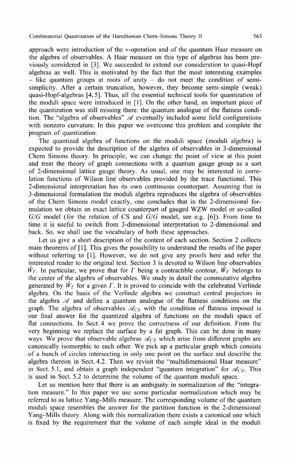
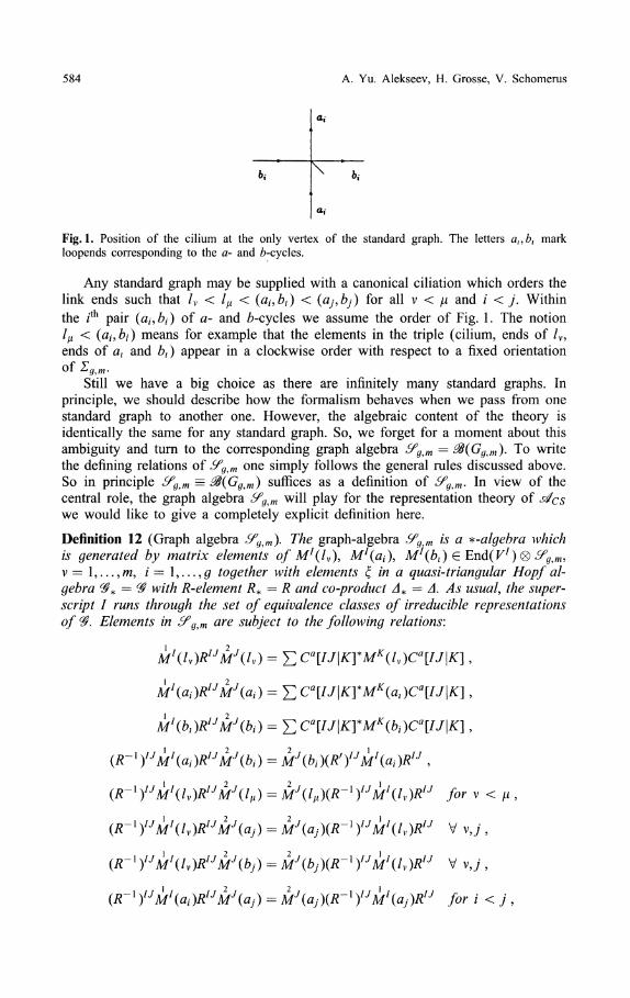
Fig. 1. Position of the cilium at the only vertex of the standard graph. The letters al,bl markloopends corresponding to the a- and ^-cycles.
Any standard graph may be supplied with a canonical ciliation which orders thelink ends such that /v < lμ < (fl/,6 z) < («/,&/) for all v < μ and / < j. Within
the /th pair (α/,6/) of a- and /^-cycles we assume the order of Fig. 1. The notionlμ < (aί>bi) means for example that the elements in the triple (cilium, ends of /v,ends of at and bt) appear in a clockwise order with respect to a fixed orientationθf Σgίfn.
Still we have a big choice as there are infinitely many standard graphs. Inprinciple, we should describe how the formalism behaves when we pass from onestandard graph to another one. However, the algebraic content of the theory isidentically the same for any standard graph. So, we forget for a moment about thisambiguity and turn to the corresponding graph algebra Sf^m = &(GCJ,m). To writethe defining relations of £fg^m one simply follows the general rules discussed above.So in principle £fg,m = $(βg,m) suffices as a definition of ,w In view of thecentral role, the graph algebra «9^>m will play for the representation theory of j/cswe would like to give a completely explicit definition here.
Definition 12 (Graph algebra ^,m). The graph-algebra ^w is a ^-algebra whichis generated by matrix elements of M7(/v), Ml(μι\ M7'(6,) e End(F7) ® m,v = !,...,/«, / = !,...,# together with elements ξ in a quasi-triangular Hopf al-gebra ^* — with R-element R* — R and co-product Δ* —A. As usual, the super-script I runs through the set of equivalence classes of irreducible representationsof . Elements in <9^m are subject to the following relations:
= ΣCa[IJ\K]*Mκ(lv)Ca[IJ\K]
MI(ai)RIJM\ai) =
M\bl)RIJMJ(bi) =
(R-lyJM!(lv)RIJMJ(lμ) = M\lμ)(R~l)IJMI(lv)RIJ for v < μ ,
(R-v)IJM\lv)RIJM\aj)=M\aj)(R-l}IJMI(lv)RIJ V vj ,
(R-λyjMI(lv)tfJM'(bj) = MJ(bj)(R-l)IJM!(lv)RIJ V vj ,
(R~ιyjMI(ai)RIJMJ(aj) = MJ(aj}(R~l yjM!(aj)B?J for i<j,
Combinatorial Quantization of the Hamiltonian Chern-Simons Theory II 585
(R-])'JMI(a,)RIJMJ(bj) = MJ(bj)(/T')IJMI(aJ)RIJ for i <j,
(R-]yjM!(bi)RIJMJ(bj) = MJ(bj)(R-[yjM1(bj)RIJ for i < j ,
-1 IJ ' / IJ 2 J 2 J -1 IJ ] I IJ
μJ(ξ)MJ(lv)=MJ(lv)μJ(ξ),
μ\ξ)MJ(ai) = MJ(ai)μ/(ξ) , μj (ξ)MJ (b,) = MJ(b^J(ξ) ,
where μ\ξ) = (τ1 0 id)(zl(O) € End(K7) 0 $ as before. With M7(-/v), M7(-αz)and M\—bt) being constructed from M7(/v), M7(βz) and Ml(b[) with the help offormula (3.10) (s0 ί/zαί M7(/V)M7(-/V) = β7 e/c.) ί/ze αcί/ow 6>/ί//e ^-operation on^0,m ^ S' ^w through
(a,)T = σκ(R'M'(-a,)(R-]y) ,
where σκ means conjugation by K (see Sect. 2 for details).
This definition requires some comments. All links of the standard graph areclosed ("loops"). This explains why all the functoriality relations have the form(3.7). The relations between generators on different loops reflect the particular cili-ation described above and follow strictly from the rules given in Sect. 2. To verifythis, one should recall that quantum lattice connections on closed links were definedin Sect. 4 as special elements in a larger lattice algebra &(G). Here G is a graphon which all loops have been divided into two (non-closed) links by introducingadditional sites on the loops. After one has gained some experience with this typeof exchange relations, the rather pedantic procedure of dividing links will becomesuperfluous.
There is one more remark we need in order to prepare for a calculation in thenext section. We saw in Proposition 2 that holonomies which are made up fromproducts of lattice connections assigned to different links satisfy the same type offunctoriality as the lattice connection U!(i) themselves. A similar property holdsfor the lattice connections M7(/) on loops /. We demonstrate this at the exampleof M7(α«), Ml(bi) G End(F7) 0 «9^m,
κγlMI(bi)MI(ai)RIJκJlM\bi)MJ(al)
. (Rl)IJCb[IJ\LγML(al)Cb[IJ\L\
= Σκ-lCa[IJ\K]*Mκ(bl)Mκ(ai)Cb[IJ\K] .
586 A. Yu. Alekseev, H. Grosse, V. Schomerus
From this one can easily derive the following formula, which is similar to Eq. (3.10):
κγλMI(bi}MI(al) = rf/tr't/^'fc/A^ . (4.9)
It will be used in Subsect. 5.2.
5. Quantum Integration
The "multidimensional Haar measure" ω : stf >—» C mentioned in Theorem 1 restrictsto a positive functional on the algebra s$cs of Chern Simons observables. Whenthe latter is properly normalized, it does not depend on the choice of the graphand thus furnishes a distinguished functional COYM : <s#cs •—» C. This functional is ageneralization of the integration measure in the lattice Yang-Mills theory. We usethis to calculate the volume of the quantum moduli space in the second subsection.
5.7. The Yang-Mills Functional ωYM. To define the functional ωYM we use thesame notations as in Sect. 3.2. In particular, the graph G which we have drawn onthe punctured Riemann surface Σ is supposed to possess M plaquettes. With thefinite real constant Jf = (]C(d/)2)~1/2 introduced in relation (3.20) we define
ωYM(A) = J^-2Mω(A) for all A e J/^} . (5.1)
Obviously, COYM inherits its positivity from the positivity of ω.
We have seen at the end of the preceding section that the algebra s$Cs = ^csdoes not depend on the graph G. The main purpose of this subsection is to establishthe graph-independence for ωγM-
Proposition 13 (Graph-independence of COYM)- Let G be a graph and suppose thatG' is a second graph so that either
1. G1 is obtained from G by dividing one link i on G into links i\,Ϊ2 on G1 byadding one additional site x on /,
2. G' is obtained from G by contracting one link ί on G so that i is removedand its endpoints are identified on G1',
3. G' is obtained from G by erasure of a link ί on the common boundary oftwo plaquettes P,P', with P containing no marked point.
Then the Yang-Mills functional OJYM for the graph G is equal to the Yang-Mills functional ωr
YM assigned to the graph G' (since in all three cases the corre-
sponding algebras s$cs — cs(G) are isomorphic to A'cs = j/^^ (G7), equalityof the functίonals is well defined).
Proof The first case is essentially trivial. It follows directly from Definition (2.23)of ω. 2. can be derived by combining the first and the last case. The simple argumentis left to the reader. In turning to the proof of 3., let ^,#' denote two curves onthe boundary of P,P' such that {^,/} and {—/, *&'} are closed. Both are assumedto move counter-clockwise. By definition, an element A in s$cs is of the formA = ecsΛ. with
fτ\ m
ecs = 4V = Π ΛP) Π/W (5.2)
Combinatorial Quantization of the Hamiltonian Chern-Simons Theory II 587
being the unit element in the moduli algebra s#cs According to Proposition 10,the element A G s$ can be written without usage of U!(±i). Given an arbitrarypresentation of A one simply has to replace UI(±i) by ί/7(=F^). In the followingwe will assume that this replacement has been made. The image of A under the
isomorphism between jtfcs and £#'Cs ^s ~ ecs^ (ecs ^s tne umt element in jtf'cs).With these notations, the statement of the proposition,
is equivalent to
Λ'-2Mω(ecsA) = -2(M-^ω(e'csA) . (5.3)
The different powers of Jf are due to the fact that G1 has one plaquette less thanG. This equation is a consequence of the following lemma.
Lemma 3. Suppose that F G stf — stf(G) does not contain elements U!(±i) with ibeing on the common boundary of two arbitrary plaquettes P, P' of G. After i isremoved, the plaquettes P,Pf merge into a single plaquette P U P' on G' — G — i.We have
ω(c\P}cJ(P')F) = (d1Γλω(cI(P^P')F)δu . (5.4)
Here cI(P),cJ(Pf) and c!(P(JP') are given by Eq. (3.19) (which holds for arbi-trary but fixed dilations).
Proof of the Lemma. We want to show first that the left-hand side of Eq. (5.4) isnonzero only for / =J. The formula (2.23) for ω reveals that the value of ω can benonzero, only if the argument has a component which contains the factor UQ(i). Theproduct cI(P)cJ(P')F contains U!(i) and UJ(-i) and these are the only elementsassociated with the link i. Now UJ(—i) can be expressed as a linear combination
of UJ (i). The "operator product" of U!(i) and UJ(i) has components proportionalto ί/°(/), if and only if / is the conjugate of J, i.e. iff / = J. So we can set / = Jfor the rest of the proof. For simplicity we will also assume that the cilia at thesites x = t(i) and y = t(—i) lie outside of both P and P' . For different positionsof eyelashes, the proof contains some additional phases ( v / ) ± l which cancel in theend. By Eqs. (3.19) and (3.18) we have
0), (5.5)
cI(Pf) = trj](UI\i)Ur(-Vf)). (5.6)
Functoriality on the link / gives
u'wu'wu'wu^-V) = Σ
If we apply tr l
q ® tr l
q to this relation, we multiply with F and evaluate the resultingexpression with ω to obtain
ω(cI(P)cJ(P')F)
= ω
588 A. Yu. Alekseev, H. Grosse, V. Schomerus
A formula similar to Eq. (3.5) allows us to rewrite the right-hand side so that itbecomes
This proves formula (5.4) and thus Lemma 3.With the explicit expressions (3.22) for the characteristic projectors and Lemma 3
we can calculate
= ^2dκdLSκJSLjω(cI(P)cJ(Pl)F)
dfrlω(cί(PυP')F)
SRΪω(cI(P U P')F)
PUP')F) . (5.7)«/?
Proof of Proposition 13 (3.) (continued). For Proposition 13, P was assumed notto contain a marked point so that it contributed with a factor χ°(P) to ecs P' wasarbitrary and so is the associated factor χL(P'). In the calculation leading to (5.7)we can set K = 0 and use
with ' meaning that the product is restricted to plaquettes nonequal to P,P' ' . Withc/o — 1 and N%L = OL,R this gives the formula (5.3) and hence proves the proposi-tion.
5.2. Volume of the Quantum Moduli Space. To demonstrate how computationscan be performed within the framework of this paper, the volume of quantummoduli space of flat connections on a marked Riemann surface Σ is calculated2. Inpractice we define the volume of the quantum space as an integral or trace of thecharacteristic projector. In the framework of the 2-dimensional lattice gauge modelone can interpret this result as a partition function of the system. As there is noHamiltonian involved, we shall get just a number.
The "characteristic function" for the quantum moduli space is the projector
ecs = 47ί} = Π xV) ΠxVv) , (5.8)
which contains one factor for every plaquette of the graph which we have drawnon the marked Riemann surface Σg^m. The 7V, v = l , . . . ,m, are the labels sittingat the m punctures. ^0 denotes the set of plaquettes without marked point. If acharacteristic function is integrated, this gives the volume of the correspondingspace. In our case, integration is defined with the help of the Yang-Mills functional
ojγM and this means that the volume of the moduli space is O)YM(^CS )• Using
the graph independence of the algebra ^^s anc* me functional ωYM, we fix a
A similar calculation was also done recently by Buffenoir and Roche [15].
Combinatorial Quantization of the Hamiltonian Chern-Simons Theory II 589
particular graph from the very beginning. Let us use the standard graph discussedin Sect. 4.2 for this purpose. This is certainly not necessary for the computationsto follow, but it simplifies the presentation and can help to make it as concrete aspossible. Before we give the general result, we would like to discuss two examples.
Example 1. Genus 0. Recall that the standard graph G^m on a Riemann spherewith m marked points consists of m loops which start and end at the same vertex.The standard graph has m + 1 plaquettes, one of which does not contain a markedpoint. So the characteristic projector is
To calculate its expectation value, one should recall the formula (5.7). It allows
to relate the expectation value of the characteristic projector e^ on the standardgraph Gm to a similar expectation value on a simpler graph, from which one linkand one plaquette has been removed. One can actually iterate this procedure to get
Here P = \J™~Q
} Λ> and we used do = 1 and N%J = δj,κ. We stopped the calculationbefore we integrate over the last link on the graph which separates the two plaquettesP and Pm. From the definition of characteristic projectors and Eq. (3.22) one infers
XK(P) = lf(Pm) Using the property χκ(Pm)χL(Pm) = δκ,Lχκ(Pm) we can treat theremaining expectation value as follows:
We made use of the normalization of (OYM on a graph with two plaquettes, thedefinition (3.22) of characteristic projectors, the property ω(c7) = <5/?0 and propertiesof the S-matrix. The result implies for the volume
' = (ΓR,)Σ<^\ V=l / Kn
Ί'2X7*1/3...»Λ.-2'»^-2κ{ "κ2
no Λ
We want to rewrite this using properties of the matrix S. To this end we insert
7V0 ιn~2 '" = ^2Sκm_2jSjιm and move the first S through the product of fusion matri-ces. This results is
(5.9)
Example 2. Genus 1 . The standard graph G\tfn has again m + 1 plaquettes. But thistime the plaquette PQ is bounded by the links /v as well as by a- and 6-cycles on
590 A. Yu. Alekseev, H. Grosse, V. Schomerus
the torus. Let us merge step by step all plaquettes into one and call it P. In thisway we erase all /v links so that the boundary of P looks as ba~{b~la. Using thesame arguments as in the first example we see that
_ . (5.10)Kμ
Observe that the boundary of P contains every link twice so that the evaluation ofω(χκ(P)) is quite nontrivial. Before one can integrate over the degrees of freedomassigned to a particular link on the graph, one has to ensure that this link appearsonly once and only in one orientation in the integrand. This can be done with thehelp of exchange relations and functoriality. Let us calculate the expectation valueof (^(P) first. To this end we insert the formula (3.19) for ^(P) and invert theorientation of the {— α, — b} in the middle. This is done with the help of Eq. (4.9).Next functoriality can be applied on the link b which then allows to perform theintegration on b. In formulas this is
= djω((MJ <g> tr7~)[M
• C[JJ\0]MJ(a)gJ])
= djω((trj ® trJ)[C[JJ\Q]*C[JJ\0]MJ\a)(RfyJC[JJ\QT
- κjω((trj
In this expression we inserted the definition (2.11) of the g -trace. Now we canintegrate on the link a. The formula
t^(MJ(a))MJ(a) = £>/[(*- V"' ' C[JJ\K}*MK(a)C[JJ\Kl\
follows from functoriality and was derived earlier in Sect. 3. It shows that
ω(tr/(MJ(α))M-/(α)) = [v^ff1 C[JJ\K]*C[JJ\K}} = vjldjl .
We may insert this into our expression for ω(c'(Po)) which then becomes
ω(cJ(P)) = dj\trj <S>trJ)[C[jJ|0]*C[jJ|0]ί7J]
= </72tr,V) = </,-'. (5.11)
With the normalization of ωγM on a graph having only one plaquette, we find
Combinatorial Quantization of the Hamiltonian Chern-Simons Theory II 591
When this is finally plugged into the formula above, we can write an expressionfor the volume,
l 2 Λ Γ 1 3 Λ T /Π— 2\ Nκ2 •••Nκm_l
J \ V—\
where the last line employs the same type of algebra described in the first example.Now we are sufficiently prepared to deal with the general case.
Proposition 14 (Volume of the moduli space). The volume of the quantum modulispace of flat connections on a compact Rίemann surface ΣCJ^m of genus g and withm punctures marked by 7V, v = l , . . . ,w evaluated with the Yang-Mills measureis given through
(5.13)
Proof. The proof of this formula is again done with a calculation on the standardgraph (70, m. The latter has m -f 1 plaquettes. When we erase all links lv we are leftwith the plaquette P which is bounded by a combination of a- and Z>-cycles whichcorresponds to Eq. (4.8). We designed the proof for the g = 1 case in such a way,that it can be applied directly to the higher genus. We leave this to the reader.Let us just do the power counting for dj. A generalization of formula (5.11) forthe value of ω(cJ(P)) shows that every pair (#/,&/) of a- and ό-cycles contributeswith a factor dj2 until only ϊτj
q(ej) is left. So the g pairs (#/,&,) together with
tΐq(ej) = dj give rise to dj~2g, i.e.
Compared to the result for the torus, this gives an extra factor of d2~2fj in the finalformula for the volume of the moduli space.
5.3. Canonical Measure and Verlinde Formula. The functional ωYM that we havediscussed so far had the fundamental properties of being gauge invariant and graphindependent. These invariances fix the functional only up to a coefficient which maydepend on the genus g, the number m of marked points, the labels 7V, v = 1, . . . , m atthe punctures and on the deformation parameter q. Actually, there exists a canonicalnormalization of the measure. This is used in the Chern Simons theory and we call itojcs- The different normalizations of ωcs and MYM can be encoded in the followingrelation:
= λ(g,m,I\,...,Im9q)ωYM . (5.14)
The aim of this subsection is to explain the choice of the positive coefficients λ.One can define the canonical normalization in two different ways. The first
approach is through the representation theory of the moduli algebra. Assume for amoment that the latter is finite dimensional (this is indeed the case for q being a rootof unity). As a *-algebra with positive inner product, the moduli algebra is semi-simple and splits into a direct sum of matrix algebras. One can fix the canonical
592 A. Yu. Alekseev, H. Grosse, V. Schomerus
functional ωcs by the requirement that -when restricted to a simple summand-itcoincides with the usual matrix trace. This approach furnishes a proper definition forωcs which is fundamental for the considerations to follow below. On the other hand,a direct computation of the canonical normalization from this definition requires thefull information about the representation theory. This is the subject of the subsequentpaper [14] where the representation theory of the moduli algebra is considered indetail.
Another approach refers to the theory of deformation quantization. Treating thedeformation parameter q as an exponent q — exp(h) of the Planck constant, one canexpand the commutation relations of the moduli algebra into formal power series inh and identify this picture with deformation quantization of the moduli space (formore details see [24]). According to the theorem of Tsygan and Nest [23] thereexists a unique canonical trace in the framework of deformation quantization. Weconjecture that this trace coincides with an expansion into the formal power seriesin h of the canonical functional ωcs defined via the representation theory.
Both ways to normalize the functional ω include some complicated analysiswhich is beyond the scope of this paper. Instead, we plan to describe a different wayto determine the coefficients λ(g,mj\^...jm,q) which characterize the canonicalfunctional ωcs This computation is based on several suggestive properties of themoduli algebra which are more natural to prove in the context of the paper [14]. Weformulate these properties as theorems labeled by latin letters. Assuming validity ofthese theorems, our method gives a derivation of the canonically functional ωcsActually, we are going to combine the ideology of the Topological Field Theoryand the algebraic approach of this paper.
Let us introduce some new notations first. Using the graph algebra correspondingto some standard graph, one can assign a bunch of matrix generators M\x) to eachcycle x on a Riemann surface. As we have discussed above, they furnish elementsc7(jc)-one for every label /-when they are evaluated with the g-trace. For thehomologically trivial cycle c, the corresponding elements c7(x) belong to the centerof the graph algebra. If the cycle x is nontrivial, they are no longer central. Theiralgebraic relations, however, remain those of a fusion algebra, i.e.
c'(X)cJ(X) = N'KJcIi(x\ (c'(X)Y=cI(X), (5.15)
K
for arbitrary cycle x. We denote this algebra by i^(x).Suppose that 3C be a subalgebra of an algebra ®/. The (relative) commutant of
3C e <& will be denoted by <g(SC,<3f).
Let jtfgtm" be a moduli algebra corresponding to a Riemann surface of genusg and with m marked points. Consider the 0-cycle ag of some standard graph andthe fusion algebra i^(ag). Without proof we state
Theorem A (Induction in the genus g}. The commutant ^(i^(ag), J^g,™""* ) splitsinto the direct sum of moduli algebras of genus g — 1 with m + 2 marked points
ΓJ f1 - (5-16)
Here the sum runs over all classes of irreducible representations of the symmetryHopf algebra.
Combinatorial Quantization of the Hamiltonian Chern-Simons Theory II 593
In the language of Topological Field Theory, evaluation of the commutant cor-responds to shrinking the cycle ag so that we get a surface of lower genus. It hastwo marked points at the place where the handle is pinched - one on either sideof the cut. Shrinking all the ^-cycles one after another, one produces spheres withm-\-2g marked points.
We apply a similar technique to reduce the number of marked points. Consider
the moduli algebra ^om corresponding to a sphere with m marked points. Pickup a cycle / = lm-\ o lm (i.e. the product of the two elementary loops lm-\ and lm)and construct the fusion algebra i^(l). As before, we investigate the commutant of
^(/) in j/ow"" The result is given by the following theorem.
Theorem B (Induction in the number m of punctures). The commutant of 1^(1) in
j^Om''"' m* splits into the direct sum of products of moduli algebras correspondingto m - 1 and 3 marked points
#(T^(/),^o wv"'/w*) - Θ^om'-ι/m~2'/} ® Q7/'""1'7'"* (5-17)7
Here the sum runs over all classes of irreducible representations of the symmetryHopf algebra.
In Topological Field Theory the evaluation of the commutant should be inter-preted as a fusion of two marked points into one. As before, one can imagine thatwe create a long neck which separates these two points from the rest of the surface.When we cut the neck, the surface splits into two pieces. The "main part" carriesthe rest of the marked points and a new one created by the cut. The other piecehas only three punctures, two of them are those that we wish to fuse and the newone appears because of the cut. Iteration of this procedure results in a product of3-punctured spheres.
In the following we will need two simple consequences of Theorems A and B.Namely, the decomposition of the commutant of the fusion algebra determines thefollowing decompositions of the unit:
β{/b..,/m} = ^e{h^im^ΐ} ?
7 &
ί7b...,7m} _ ί7lv..,w} ^Jΰπ-iΛ,}
Here e}}^ denotes the unit of the moduli algebra s$\^ The equations are a simpleconsequence of the completeness of characteristic projectors, i.e. of Σ/Λ*) = id.
Now we can turn back to the discussion of the canonical functional cocs- Bydefinition, it is supposed to coincide with a usual matrix trace. When the standardproperties of a matrix trace are combined with the decomposition formulas for the
units egtm'"' » one arrives at
594 A. Yu. Alekseev, H. Grosse, V. Schomerus
By iterations, these equations reduce the evaluation of o)cs(eg,m ) to the knowledge
of ωcs(eQJ3K) This has a simple geometric interpretation. The algebraic informationin Theorem A and B about the decomposition of the commutant and the definitionof the canonical functional ωcs as the standard matrix trace mean that the volumeof the quantum moduli space does not change under pinching when it is evaluatedwith the canonical measure ωcs Using this invariance, one can first decomposethe moduli space according to the decomposition of a punctured Riemann surfaceinto 3 -punctured spheres and then calculate the volume directly as a function of thevolume of the quantum moduli-space assigned to the 3-punctured sphere, i.e. as a
function of ωcs
In the algebraic context, the numbers c o c s ' ' ) nave to ^e determined fromthe representation theory. For this we anticipate the following simple result (a proofwill be given in [14]).
Theorem C (3-punctured sphere). The moduli algebra ^ corresponding to a 3-
punctured sphere is ίsomorphίc to a full matrix algebra of the dimension d =
This means that the canonical functional ωcs obeys
Putting all this together, the normalization of ωcs is completely determined, i.e.
tt>cs(eg,m ) can be calculated. After rewriting everything in terms of the matrix S,the result is
J \J=l^
In particular, for a surface of genus g without marked points one recovers thefamous Verlinde formula,
j
These formulas have to be compared with the corresponding formula for ωYM inProposition 14. From this comparison one infers
λ(g, m,Iι9...9Im9q) = 2~2g [dι . (5.20)\ / /
Let us note that the Verlinde formula has been designed to compute the numberof conformal blocks in the WZW model. Witten related the space of conformalbolcks to the space of holomorphic sections of the quantum line bundle over themoduli space of flat connections. The latter is a natural Hubert space associated toquantization of the moduli space by geometric quantization. We deal with anotherquantization scheme which associates to the moduli space a quantized algebra offimctions. In this approach, the Hubert space arises as a representation space ofthe moduli algebra. Actually, the canonical trace functional evaluated at the unitelement of the algebra provides a dimension provided by the Verlinde formula.Equation (5.19) proves that this is indeed the case.
We get another interpretation of formula (5.19) if we switch to the point ofview of the two-dimensional lattice model. Then the canonical trace gives a partitionfunction of the lattice gauge model with the quantum gauge group. As this partition
Combinatorial Quantization of the Hamiltonian Chern-Simons Theory II 595
function coincides with the Verlinde number, it is natural to conjecture that thelattice gauge model at hand is an exact lattice approximation of the gauged WZWmodel (also called the G/G model). This is supported by the fact that the gaugedWZW model is equivalent to the CS model on the manifold which is a product ofa Riemann surface and a circle. To establish the equivalence one should considerarbitrary correlation functions. The partition function is the simplest among them.We do not go into detailed consideration in this paper.
6. Generalization to Quasi-Hopf Symmetries
All the theory developed above was valid under the assumption that the symmetryalgebras yx are semisimple. It is well known that this requirement is not satisfied forthe quantum group algebras Uq(&) when q is a root of unity. To treat this importantcase we proposed (cp. [1]) to use the semisimple truncation of Uq(f&\ qp = 1,which has been constructed in [5]. in this truncation, semisimplicity is gained inexchange for co-associativity, i.e. the truncated Uq(&) of [5] are only quasi-co-associative. In addition, the co-product A of these truncated structures is not unitpreserving (i.e. A(e)ή=e®e). This leads to a generalization of Drinfeld's axioms[10] which was called "weak quasi-Hopf-algebra" in [5]. To fulfill our program,we have to explain how the theory of Sects. 2 to 5 generalises to (weak) quasi-Hopf algebras. In order not to clutter the presentation, we decided to outline proofswithout conceptual significance in a separate appendix.
In the quasi-Hopf context, there appear three additional distinguished elementsassociated with the local gauge symmetry <gx. These are the elements aX9βx G &x andthe re-associator φx — 3?x 0 &x 0 &x. The re-associator φx satisfies the fundamentalrelation
φx(Δx ® id)Δx(ξ) = (id ® Δx)Δx(ξ)φx for all ξ € <3X
and is quasi-invertible in the sense that
φxφ~λ = (id <g) Ax)Ax(e)9 φ~λ φx = (Δx ® \ά)Δx(e) .
Following DrinfeΓd, (x.X9βx are required to obey
&(£)*& = *xex(ξ), ξl
σβxyx(ξl) = βA(ξ),
ψlβx£fx(φ2
xσ)*xφlσ = e, ^X(φl
xσ)axφ2
xσβx^x(φl) = e ,
with ζσ,φxσ,φxσ being defined through the expansions of Ax(ξ)9φX9φx — φ~λ asusual. As remarked in [1], consistency with the *-operation means
Details and further relations can be found elsewhere (see e.g. [1] and referencestherein).
An element ux G x is defined by relations similar to (2.1),
Notice that the second equation follows from the first by taking adjoints. ux andthe ribbon element vx G &x continue to satisfy vx = ux^x(ux). All other relations(2.2,2.3) of the ribbon element remain true as well. As for ribbon-Hopf algebras,
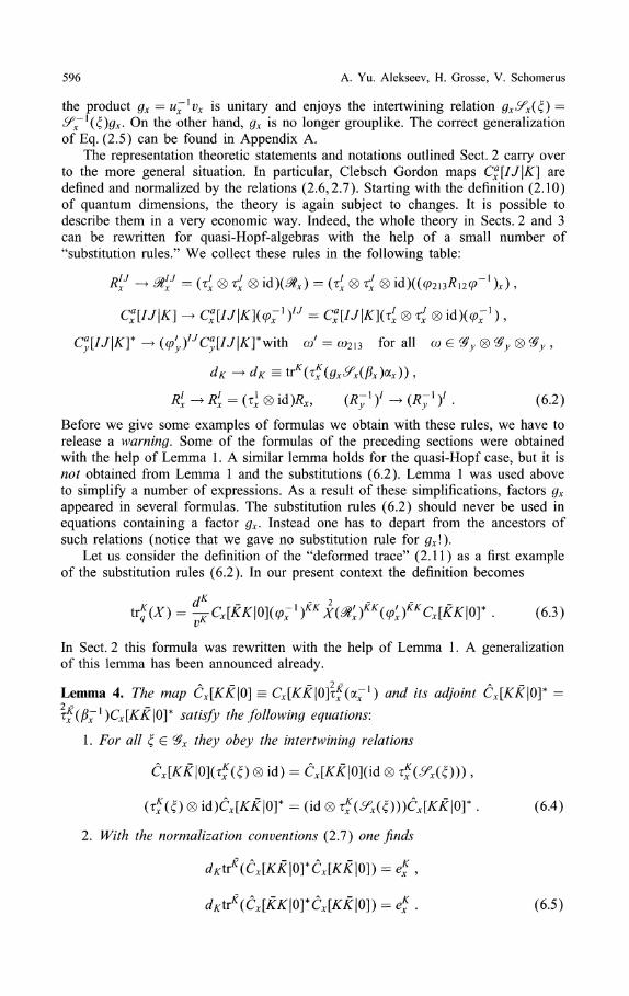
596 A. Yu. Alekseev, H. Grosse, V. Schomerus
the product gx = u~lvx is unitary and enjoys the intertwining relation gx^x(ξ) =On the other hand, gx is no longer grouplike. The correct generalization
of Eq. (2.5) can be found in Appendix A.The representation theoretic statements and notations outlined Sect. 2 carry over
to the more general situation. In particular, Clebsch Gordon maps CX[IJ\K] aredefined and normalized by the relations (2.6,2.7). Starting with the definition (2.10)of quantum dimensions, the theory is again subject to changes. It is possible todescribe them in a very economic way. Indeed, the whole theory in Sects. 2 and 3can be rewritten for quasi-Hopf-algebras with the help of a small number of"substitution rules." We collect these rules in the following table:
R(J -> &X
J = (τί ® ® id)(ΛΛ) - (τ^Θ r, <g> id)((φ2i3R\2φ'l)x) ,
C;[IJ\K] - Ca
x[IJ\K](φx
lyj = Ca
x[IJ\K}(τ!
x ® < ®
Ca
y[IJ\K]* -> (φ'yyjCa
y[IJ\K]*with ω' = ω2ι3 for all ω
> (Λ;1 / . (6.2)
Before we give some examples of formulas we obtain with these rules, we have torelease a warning. Some of the formulas of the preceding sections were obtainedwith the help of Lemma 1 . A similar lemma holds for the quasi-Hopf case, but it isnot obtained from Lemma 1 and the substitutions (6.2). Lemma 1 was used aboveto simplify a number of expressions. As a result of these simplifications, factors gx
appeared in several formulas. The substitution rules (6.2) should never be used inequations containing a factor gx. Instead one has to depart from the ancestors ofsuch relations (notice that we gave no substitution rule for gx\).
Let us consider the definition of the "deformed trace" (2.11) as a first exampleof the substitution rules (6.2). In our present context the definition becomes
tή(X) = ^Cx[KK\0](φ-lfκX(^'xfκ(φ'xf
κCx[KK\OT (6.3)
In Sect. 2 this formula was rewritten with the help of Lemma 1 . A generalizationof this lemma has been announced already.
Lemma 4. The map CX[KK\0] = Cx[KK\0]τj (α~ !) and its adjoint CX[KK\Q]* =
τx(β~l)Cx[KK\Q]* satisfy the following equations:
1. For all ξ G &x they obey the intertwining relations
Cx[KK\ϋ\(τ*(ξ) Θ id) = Cx[KK\0](id ® τ?(^(£))) ,
(τf (ξ) ® id)Cx[KK\θr = (id ® τ*(ίex(ξ)))Cx[KK\0\* . (6.4)
2. With the normalization conventions (2.7) one finds
= eκ
x ,
= eκ
x . (6.5)
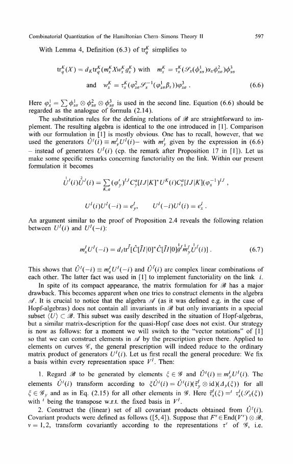
Combinatorial Quantization of the Hamiltonian Chern-Simons Theory II 597
With Lemma 4, Definition (6.3) of tr^ simplifies to
) with n£ = τ?(yx(ώ*)oίxώln)ώ*
and wf = ^(φ2
xσ^χ-[(φlβx))φlσ. (6.6)
Here q>χ = Σ Φxσ ® Φxσ ® Φxσ is used in me second line. Equation (6.6) should beregarded as the analogue of formula (2.14).
The substitution rules for the defining relations of $ are straightforward to im-plement. The resulting algebra is identical to the one introduced in [1]. Comparisonwith our formulation in [1] is mostly obvious. One has to recall, however, that weused the generators ϋl(ι) = m!
yU!(i)- with m!
y given by the expression in (6.6)
- instead of generators U!(i) (cp. the remark after Proposition 17 in [1]). Let usmake some specific remarks concerning functoriality on the link. Within our presentformulation it becomes
i/7(Ot/7(-o = 4, i/7(-/)i/7(i) = 4 .An argument similar to the proof of Proposition 2.4 reveals the following relationbetween £/7(ι) and U'(-i):
ntxU!(-i) = d^ClϊIlOYCίϊIlOm^U^i)] . (6.7)
This shows that U!(-i) = w7t/7(-z) and Uf(i) are complex linear combinations ofeach other. The latter fact was used in [1] to implement functoriality on the link /.
In spite of its compact appearance, the matrix formulation for & has a majordrawback. This becomes apparent when one tries to construct elements in the algebraj/. It is crucial to notice that the algebra stf (as it was defined e.g. in the case ofHopf-algebras) does not contain all invariants in $ but only invariants in a specialsubset (U) C &. This subset was easily described in the situation of Hopf-algebras,but a similar matrix-description for the quasi-Hopf case does not exist. Our strategyis now as follows: for a moment we will switch to the "vector notations" of [1]so that we can construct elements in sϋ by the prescription given there. Applied toelements on curves #, the general prescription will indeed reduce to the ordinarymatrix product of generators Ul(i\ Let us first recall the general procedure: We fixa basis within every representation space V1 . Then:
1. Regard Si to be generated by elements ξ G and U'(i) = ml
yU!(i). The
elements U*(i) transform according to ξU*(i) = ί/7(/)(τ7 0 i d ) ( A y ( ξ ) ) for all
ξe^y and as in Eq. (2.15) for all other elements in . Here τ*x(ξ) =' τ7(^(0)with l being the transpose w.r.t. the fixed basis in V1 ' .
2. Construct the (linear) set of all covariant products obtained from U!(i).Covariant products were defined as follows ([5,4]). Suppose that Fv GEnd(K v) 0 ,v = 1,2, transform covariantly according to the representations τv of $, i.e.
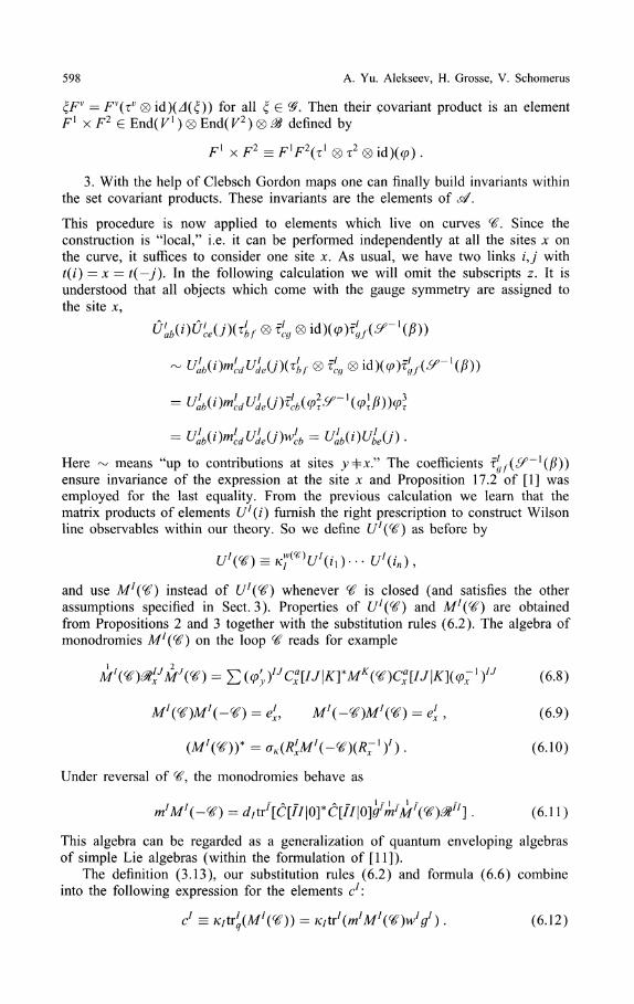
598 A. Yu. Alekseev, H. Grosse, V. Schomerus
ξFv = Fv(τv 0 id)( j(£)) for all ξe&. Then their covariant product is an elementF1 x F2 E EndCK1 ) 0 End(K2) <g> <# defined by
F1 x F2 = F'FV 0 τ2 0 id)(φ) .
3. With the help of Clebsch Gordon maps one can finally build invariants withinthe set covariant products. These invariants are the elements of stf .
This procedure is now applied to elements which live on curves (6. Since theconstruction is "local," i.e. it can be performed independently at all the sites c onthe curve, it suffices to consider one site x. As usual, we have two links ij witht(i) = x — t(—j). In the following calculation we will omit the subscripts z. It isunderstood that all objects which come with the gauge symmetry are assigned tothe site x,
Here ~ means "up to contributions at sites jyφx." The coefficients τ(jf(^ensure invariance of the expression at the site x and Proposition 17.2 of [1] wasemployed for the last equality. From the previous calculation we learn that thematrix products of elements U!(i) furnish the right prescription to construct Wilsonline observables within our theory. So we define (77(^) as before by
and use M7(^) instead of f/7(^) whenever ^ is closed (and satisfies the otherassumptions specified in Sect. 3). Properties of U1^) and M7(^) are obtainedfrom Propositions 2 and 3 together with the substitution rules (6.2). The algebra ofmonodromies M7(^) on the loop ^ reads for example
l)IJ (6.8)
(6.9)
(6.10)
Under reversal of , the monodromies behave as
. (6.1 1)
This algebra can be regarded as a generalization of quantum enveloping algebrasof simple Lie algebras (within the formulation of [11]).
The definition (3.13), our substitution rules (6.2) and formula (6.6) combineinto the following expression for the elements c1:
cl = /c/tr7(M7(^)) = κ:/tr/(m/M7(^)w7^7) . (6.12)
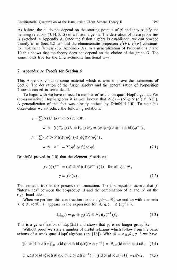
Combinatorial Quantization of the Hamiltonian Chern-Simons Theory II 599
As before, the c1 do not depend on the starting point x of ^ and they satisfy thedefining relations (3.14,3.15) of a fusion algebra. The derivation of these propertiesis sketched in Appendix A. Once the fusion algebra is established, we can proceedexactly as in Sect. 3.2 to build the characteristic projectors %!(P) XQ(P) continuesto implement flatness (cp. Appendix A). In a generalization of Propositions 7 and10 this shows that the theory does not depend on the choice of the graph G. Thesame holds true for the Chern-Simons functional
7. Appendix A: Proofs for Section 6
This Appendix contains some material which is used to prove the statements ofSect. 6. The derivation of the fusion algebra and the generalization of Proposition7 are discussed in some detail.
To begin with we have to recall a number of results on quasi-Hopf algebras. For(co-associative) Hopf-algebras it is well known that A ( ξ ) = (if 0 ^)Δ'(<f~\ζ}).A generalization of this fact was already noticed by DrinfeΓd [10]. To state hisobservation we introduce the following notations:
with Σ Tσ 0 Uσ 0 Vσ 0 Wσ = (φ 0 e)(Δ 0 id 0 idXφ"1 ) ,
/ = Σ (^ ® y)(A'(Φl
σ))yA(φ2
σβ&(φl)) ,
With φ-l=ΣΦlσ®Φ2σ®Φl (7.1)
DrinfeΓd proved in [10] that the element / satisfies
fA(ξ)f~l =(&><& ^)(A'(^-l(ξ)) for aΆ ξe& ,
Ί - /Λ(α) . (7.2)
This remains true in the presence of truncation. The first equation asserts that /"intertwines" between the co-product A and the combination of A and £f on theright-hand side.
When we perform this construction for the algebras ^ we end up with elementsfx £ &x ® jc fx appears in the expression for Δx(gx) = Δx(u~lvx),
AM = gx® gx(^x ® X/Γ1)/, (7.3)
This is a generalization of Eq. (2.5) and shows that gx is no longer grouplike.Without proof we state a number of useful relations which follow from the basic
axioms of a weak quasi-Hopf algebras (cp. [16]). With ^ = φ2i3^i2φ~1 we have
[(id 0 id 0 Λ)(φ)]23i4(id 0 A 0 id)(3t)(e 0 φ~l ) = ι34(id 0 id 0 Δ)St , (7.4)
0id0id)(^)(id0id0 JXφ" 1 ) = [(id 0 id 0 Λ)(^)] 1324^234 . (7.5)
600 A. Yu. Alekseev, H. Grosse, V. Schomerus
These two relations are in fact equivalent to Drinfeld's pentagon and hexagon equa-tions. If we use m = £f(φ[
σ)oίφ^ ® φ% and w = φ2
σ^~λ(φl
σβ) ® φ\ as before then
(id ®Δ)Δ(φl)(ιά <8> Δ)(w)(e <8>
= φ(Δ (8) id)(w) , (7.6)
Γ\<f <8> 50(<p* <g) <^)(e 0 m)(id o J)(/ιι)(id ® Δ)Δ(φ3
σ)
= (Δ®\A)(ni)φ-λ . (7.7)
Here f = Σfσ®fl is the element (7.1) and /' = Σ/2®/i of course> a11
these relations hold also "locally" at the sites x of the graph.We are now prepared to prove the basic properties of the elements c1 G #0
defined in (6.12).
Independence of x . The definition of c1 depends on the curve # on the boundaryof the plaquette P through the site x at which ^ starts and ends. We want to showthat c1 does not change, if we use the site y E dP instead of x. As in the proofof Proposition 4 we break the curve ^ at an arbitrary point y on dP and use thebraid relations
11^1). (7.8)From Eq. (7.4) one obtains
e 0 mz = (e ® ^Z(p2
zσ) 0 e)[(iά 0 Az)(mz)]2i3@z(plσ ® ^z(/4)) (7.9)
with ^z = Σplσ ®Pzσ ®Pzσ This relation and the co variance properties (2.15)furnish
Now we use the equation
to cancel the factors mz in between the two factors U1 . Then one multiplies the twocomponents of Eq. (7.10) and evaluates the trace tr7 of the product. To simplify theresulting expression, the formula
) 0 e)
is inserted. This leads to
trVXC^1)^2)^') = tr'ίmX^^VX) ,
which establishes the independence of c1 on the choice of the site x on dP.
Combinatorial Quantization of the Hamiltonian Chern-Simons Theory II 601
Fusion algebra. The derivation of the fusion algebra in the quasi-Hopf case departsfrom the "operator products" of monodromies
λ)IJ . (7.10)
Let us omit the subscript x for the rest of this section. Together with the covarianceof monodromies, μl(ζ)Ml(<$} = M7(^)μ7(O for all ξ E &X9 the formula (7.9) canbe used to convert the factor $ on the left-hand side of the operator product intoa factor m,
j J 2 Θ β ®
From here we can calculate e'er7 using the relation (6.12) and
(p\ ® A(pl))(e ® w)(e ® -'(Pσ) ® e) = ^T1 [(id 0 J)w]213
together with Eqs. (7.6,7.7). The result of a short calculation is
c!cj = K/K /Σί f r 7 ®trJ)[(ffyJCa[IJ\K]*mκMκ((g)wκ
^-1 0 5^-1)(/-1))/'/ flf7 9J]
(tr7 0 tτJ)[Ca[IJ\KγmκMκ(^)wκgκCa[IJ\K](R-l)IJ] .
The last equality is a consequence of Eq. (7.3). The fusion algebra clcj =finally follows from the normalization (2.7).
Evaluation of (c7)* is left as an exercise. As an intermediate result one shows
Then relation (6.11) is inserted. After application of Lemma 4 one uses Eq. (6.1)
and writes 3t as a product φ2i3^i2φ~1 This gives the result (c7)* = cl .
Flatness. Every line in the prrof of Proposition (7) can be "translated" with thesubstitution rules (6.2). There is only one problem. In the second part of the proof(i.e. after Lemma 2) we exploit the completeness (3.27) of Clebsch Gordon maps,which fails to hold in the case of truncation. Even though completeness was thefastest way to get the desired results, it is not necessary. In fact, (quasi )-associativityof the co-product does suffice. We want to show this with φ = e 0 e 0 e. The caseof nontrivial φ is again obtained with the rules (6.2). From associativity of thetensor product of representation it follows that
eJCx[KK\0] = Σ Fab(I J K)Cb
x[ΪK\J]Ca
x[JK\ϊ] .
602 A. Yu. Alekseev, H. Grosse, V. Schomerus
The complex coefficients are a subset of 6j-symbols. We may use the normalization(2.7) to rewrite this as
κ)cb
x[ϊκ\j].
These two formulas can be inserted into the first equation after relation (3.27) andfurnish an alternative calculation of χ°MJ. It does not use the completeness (3.27)and remains valid in the case of truncation.
8. Discussion and Outlook
In this paper we have introduced a new quantum algebra. It is natural to interpretit as a quantized algebra of functions on the moduli space of flat connections (modulialgebra). This algebra plays the role of the observable algebra in the HamiltonianChern Simons theory. The construction of the moduli algebra requires a quasi-triangular ribbon *-Hopf algebra to be used as a gauge symmetry. A lot of examplesof such symmetry algebras are provided by quantized universal enveloping alge-bras of simple Lie algebras. Given a Riemann surface of genus g with m markedpoints, a simple Lie algebra, a onumber q being some root of unity and a setof m representation-classes [/v] of the corresponding quantized universal envelop-
ing algebra, one can construct the moduli algebra <$$ c$ . This means that we havecompleted the program of deformation quantization of the moduli space and nowwe are going to discuss perspectives of the combinatorial approach to quantizationof the Chern Simons model.
The main question which arises naturally is the comparison to other quanti-zation schemes already applied to Chern Simons theory. Among them we pick uptwo approaches which are the most suitable for comparison. These are geometricquantization [17,18] and the Conformal Field Theory approach which was usedoriginally to solve the Chern Simons model [19]. Both these approaches use theHamiltonian picture of quantization. So, their results may be easily compared to theresults of combinatorial approach.
Opening the list of unsolved questions we start with
1. Compare results of geometric quantization and the Conformal Field Theoryapproach to combinatorial quantization.
Geometric quantization as well as Conformal Field Theory produces the Hubertspace of the Chern Simons model rather than the observable algebra. In the Confor-mal Field Theory approach, vectors in the Hubert space are identified with conformalblocks of the WZW model. More precisely, they come as solutions of a certain sys-tem of linear differential equations. In the case of the Riemann sphere this systemof equations was discovered in [20] and called the Knizhnik-Zamolodchikov equa-tion. For higher genera it was considered in [21,17] etc. Geometric quantizationprovides a more abstract picture of the Hubert space. There it appears as a spaceof holomorphic sections of the quantum line bundle over the moduli space. It ispossible to find a contact between these two pictures, of the Hubert space. The keyobservation is that each complex structure on the underlying Riemann surface pro-
vides a complex structure on the moduli space. Thus, the δ-operator in the quantumline bundle depends on this complex structure. One can think that for each complexstructure on the surface we get its own geometric quantization and its own Hubert
Combinatorial Quantization of the Hamiltonian Chern-Simons Theory II 603
space. One needs a projectively flat connection on the space of complex structuresin order to identify these bunch of Hubert spaces with the unique Hubert spaceof the quantum theory. Here one makes a bridge with the Conformal Field Theoryapproach. It appears [17] that the linear system of equations for conformal blocksmay be reinterpreted as a covariance conditions with respect to some projectivelyflat connection.
While these approaches to quantization provide Hubert spaces, our combinatorialquantization provides an algebra of observables. The natural route for comparisonis to realise the algebra of observables in given Hubert spaces. This is the secondpoint in our list.2. Represent the moduli algebra in the Hubert spaces of the Chern-Simons theoryprovided by geometric quantization and Conformal Field Theory.
In principle, this is the central question of the whole program and-providedit is done-one can stop here. However, there are a couple of questions that oneshould add to the list. The first one concerns the action of the mapping class group.It is known that the project!ve representation of the mapping class group acts inthe Hubert space of the Chern-Simons theory. This representation proves to beuseful in constructing invariants of 3-manifolds. One can try to relate this idea tothe moduli algebra.3. Construct the action of the mapping class group on the moduli algebra.
The last question which we would like to mention here concerns a very par-ticular application of the machinery that we have developed. It has been recentlyproven that the relativistic analogue of the Calogero-Moser integrable model maybe naturally realized on the moduli space of flat connections on a torus with amarked point [22]. It would be interesting to develop this idea from the point ofview of the moduli algebra.4. Work out details for the example of a torus with a marked point.
We are going to consider the listed problems in the forthcoming paper [14].
Acknowledgements. It is a pleasure to acknowledge the hospitality of the Erwin SchrόdingerInternational Institute in Vienna which helped a lot to initiate this work. A.A. wants to thankthe Physics Department at Harvard University and the II. Institut fΐir Theoretische Physik of theUniversitat Hamburg for their hospitality. The work of V.S. was partly supported by theDepartment of Energy under DOE Grant No. DE-FG02-88ER25065. A.A. was supported bythe Swedish Natural Science Research Council (NFR) under the contract F-FU 06821-304. Thework of H.G. was done in the framework of the project P8916-PHY of the "Fonds sur Fόrderungder wissenschaftlichen Forschung in Osterreich".
References
1. Alekseev, A. Yu., Grosse, H., Schomerus, V.: Combinatorial quantization of the HamiltonianChern Simons thoery. HUTMP 94-B336, Commun. Math. Phys. (in press)
2. Fock, V.V., Rosly, A.A.: Poisson structures on moduli of flat connections on Riemann surfacesand r-matrices. Preprint ITEP 72-92, June 1992, Moscow
3. Boulatov, D.V.: g-deformed lattice gauge theory and three manifold invariants. Int. J. Mod.Phys. A8, 3139 (1993)
4. Mack, G., Schomerus, V.: Action of truncated quantum groups on quasi quantum planes anda quasi-associative differential geometry and calculus. Commun. Math. Phys. 149, 513 (1992)
5. Mack, G., Schomerus, V.: Quasi Hopf quantum symmetry in quantum theory. Nucl. Phys.B370, 185 (1992)
604 A. Yu. Alekseev, H. Grosse, V. Schomerus
6. Gerasimov, A.: Localization in GWZW and Verlinde formula. Uppsala preprint HEP-TH/9305090
7. Verlinde, E.: Fusion rules and modular transformations if 2D conformal field theory. Nucl.Phys. B300, 360 (1988)
8. Blau, M., Thompson, G.: Derivation of the Verlinde formula from Chern-Simons Theory andG/G model. Nucl. Phys. B408, 345 (1993)
9. Reshetikhin, N., Turaev, V.G.: Ribbon graphs and their invariants derived from quantumgroups. Commun. Math. Phys. 127, 1 (1990)
10. DrinfeΓd, V.G.: Quasi Hopf algebras and Knizhnik Zamolodchikov equations. In: Problems ofmodern quantum field theory. Proceedings Alushta 1989, Research reports in Physics. Berlin,Heidelberg, New York: Springer, 1989; DrinfeΓd, V.G.: Quasi-Hopf algebras. Leningrad. Math.J. Vol. 1, No. 6 (1990)
11. Reshetikhin, N., Semenov-Tian-Shansky, M.: Lett. Math. Phys. 19, 133 (1990)12. Frohlich, J., Gabbiani, F.: Braid statistics in local quantum theory. Rev. Math. Phys. 2, 251
(1991)13. Reshetikhin, N., Turaev V.G.: Invariants of 3-manifolds via link polynomials and quantum
groups. Invent. Math. 103, 547 (1991)14. Alekseev, A. Yu., Schomerus, V.: Representation theory of Chern Simons observables. Preprint
HUTMP 95-B342, ?-alg 950301615. Buffenoir, E., Roche, Ph.: Two dimensional lattice gauge theory based on a quantum group.
Commun. Math. Phys. 170, 669 (1995)16. Schomerus, V.: Construction of field algebras with quantum symmetry from local observables.
Commun. Math. Phys. 169, 193 (1995)17. Axelrod, S., Delia Pietra, S., Witten, E.: Geometric quantization of Chern-Simons gauge the-
ory. J. Differential Geometry 33, 787 (1991)18. Gawedzki, K.: SU(2) WZNW model at higher genera from gauge field functional integral.
St.-Petersburg Math. J. (to appear)19. Witten, E.: Quantum field theory and the Jones polynomial. Commun. Math. Phys. 121, 351
(1989)20. Knizhnik, V.G., Zamolodchikov, A.B.: Current algebra and Wess-Zumino model in two
dimensions. Nucl. Phys. B247, 83 (1984)21. Bernard, D.: On the Wess-Zumino-Witten Models on Riemann surfaces. Nucl. Phys. B309,
145 (1988)22. Gorsky, A., Nekrasov, N.: Relativistic Calogero-Moser model as gauged WZW theory. Nucl.
Phys. B436, 582 (1995)23. Nest, R., Tsygan, B.: Algebraic index theorem. Commun. Math. Phys. (to appear)24. Andersen, J., Mattis, J., Reshetikhin, N.: In preparation
Communicated by G. Felder
Related Documents