MATHEMATICAL MODELLING OF CHEMICAL ...Mathematical modelling of chemical engineering systems 771 three-dimensional problems, but approximations to these can be obtained by solving

Comput. Math..4pplic. Vol. 15, No. 9, pp. 769-794, 1988 0097-4943/88 $3.00+0.00 Printed in Great Britain. All rights reserved Copyright © 1988 Pergamon Press plc

M A T H E M A T I C A L M O D E L L I N G O F C H E M I C A L

E N G I N E E R I N G S Y S T E M S BY F I N I T E E L E M E N T

A N A L Y S I S U S I N G P D E / P R O T R A N

P. L. MILLS and P. A. RAMACHANDRAN ~Monsanto Company, Central Research Laboratory, St Louis, MO 63167, U.S.A.

~Vashington University, Department of Chemical Engineering, St Louis, MO 63130, U.S.A.

(Received 8 October 1987)

Communicated by E. Y. Rodin

Abstract--The use of commercially available software for obtaining finite-element solutions to partial differential equations encountered in engineering and the applied sciences is considered. A particular software package called PDE/PROTRAN that can solve a general class of either time-dependent, steady-state, or eigenvalue type PDEs in two space dimensions is examined from both a theoretical and practical perspective. To illustrate the application of PDE/PROTRAN, two example problems that have an origin in the engineering sciences are posed and translated into a working computer code. Solutions to these mathematical models, which describe diffusion-reaction phenomena and fluid dynamics, are also given and compared to previous solutions where available. Some advantages and limitations of the program and possible enhancements are also discussed.

I N T R O D U C T I O N

Mathematical models for many systems that are encountered in engineering, physics, and other applied sciences are often developed by applying various laws that describe the conservation of mass, momentum, and energy [1]. In their microscopic form, these models are usually given as a single or set of ordinary or partial differential equations along with appropriate initial and boundary conditions which apply over the region R and the boundary t~R. Solution of these equations using appropriate analytical or numerical methods provides local numerical values for the dependent variables of interest, such as fluid velocity, pressure, species concentration, temperature, force and electric potential. Due to the mathematical complexities of most problems, numerical techniques based upon finite differences [2-4], the method of lines [5-12], the method of weighted residuals [4, 13-21], and the finite element method [4, 16, 17, 21-33] are often used to solve the equations to obtain approximate values for these dependent variables. Among these various methods, the finite element method (FEM) is perhaps the most general since it can be applied to both linear and nonlinear model equations posed on regular or irregular regions. However, it is well known that translation of a set of model equations into a working computer code that implements the FEM can be extremely tedious and time consuming [27-29] which represents a disadvantage.

Application of the FEM to specific types of problems in engineering, such as structural analysis, fracture mechanics, heat transfer, and fluid mechanics, over the past 20-30 years has resulted in the development of a variety of commercial software packages which relieve user's from developing problem specific computer codes. Examples of these codes include ADINA, ANSYS, ASKA, FIDAP, FLUID, MARC, NASTRAN, PROBE, SAP, and TITUS [34-39]. Most of these programs are designed to solve a specific form or general set of conservation equations, for example, the linear equations of elasticity or the Navier-Stokes equations. Unfortunately, many are awkward and tedious to use due to their design which includes outdated methods for input of problem parameters and other simulation data, lack of modem graphics software for visual display of intermediate and final results, and insufficient input and run-time error checking, to name a few. Scientists and engineers who have a working knowledge of the finite element method, yet are primarily interested in focusing their efforts upon developing realistic mathematical models versus developing FEM computer software, may find that the above packages are not very appealing as a result.

769

770 P.L. MILLS and P. A. RAMACHANDRAN

Recently, a more modern computer software package that implements the finite element method on a general class of partial differential equations has become available. This package, which is called PDE/PROTRAN, is part of the IMSL family of mathematical software and has some advanced features which make it more attractive from a users perspective. The principle objective of this paper is to introduce scientists, engineers and students who are interested in using the finite element method as a mathematical modelling tool to the use of PDE/PROTRAN. Another objective is to illustrate usage of the package through selected example problems from engineering applications that may be useful to both industrial technologists and to instructors when using or teaching the finite-element method as part of courses on applied mathematics or mathematical modelling. The particular examples given here are primarily based upon chemical engineering applications, but this should not be viewed as a limitation since PDE/PROTRAN is designed to be of general applicability. Some examples from other fields are given elsewhere [41, 42] to which the interested reader is referred.

THE PDE/PROTRAN CODE

The PDE/PROTRAN package is part of the International Mathematical Subroutine Library (hereafter abbreviated as IMSL) and represents an improvement over its predecessor which was called TWODEPEP. The principle improvement was the addition of a powerful preprocessor that allows the user to specify the problem to be solved through descriptive program statements. These statements are called PROTRAN by IMSL due to their similarity to certain aspects of FORTRAN. The format and structure for some of these will be introduced through the examples that are given later. A more detailed description is available in the IMSL manual [40] and in the monograph of Sewell [41].

An attractive feature of PDE/PROTRAN is that it can be used to solve a set of partial differential equations containing a maximum of nine dependent variables t7 which depend upon the spatial coordinates x and y and time t. The general forms of these equations and the associated boundary conditions are given below for the three classes of problems for which PDE/PROTRAN is designed to solve.

(1) Steady-state problems:

O=Ax(x,y,~,~x,~y)+l~y(X,y,~,~x,~y)+F(x,y, ft,~x,~y) in R; (la)

~=Fb(x,y) on ~3Rt; (lb)

Anx+Bny=Crb(x,y,~ ) on t3R 2. (lc)

(2) Time-dependent problems:

C(x,y,t, ft)~,=Ax(X,y,t,~,tJ~,gty)+By(x,y,t,~,ftx,~y)+l~(x,y,t, ft, f~x,~y) in R; (2a)

---- Fb(X, y, t) on ~Rl; (2b)

-4nx + nny = ab(x ,y , t, ~) on OR2; (2c)

tT=Oo(x,y) at t=to. (2d)

(3) Eigenvalue problems:

o=gx(x,y ,a ,~,ay)+l~y(x,y ,a , ax, ay)+F(x,y,a,a~,ay)+2P(x,y)f~; (3a)

u = 0 on ORi; (3b)

.4nx + Bny = Gb(x, y, a) on OR 2. (3c)

The subscripts x, y, and t in the above equations denote partial derivatives in the spatial coordinates or time, while the subscript b is used to designate a function on the boundary. The unit normals on the boundary OR 2 a r e given by nx and ny where the outward direction is positive which is consistent with the usual convention. Appropriate definitions for the components of ,4, /~, C', and / r allows specific forms of various conservation laws that are typically encountered in engineering and the applied sciences to be developed. PDE/PROTRAN cannot be used to solve

Mathematical modelling of chemical engineering systems 771

three-dimensional problems, but approximations to these can be obtained by solving a series of two-dimensional problems in the plane of the third coordinate. This represents one limitation of the package, but it is not significant since many practical problems can be defined in one or two spatial coordinates.

Development of the working equations needed to solve equations (l)-(3) and the computer algorithms used to obtain the numerical results are explained in detail by Sewell [41] so that a description of the key results will be given here. Emphasis will be placed upon the steady-state and time-dependent systems described by (1) and (2) since these are the ones most often encountered in applications.

Solution of the steady-state system

Solution of the steady-state system described by (laj(lc) is initiated by assuming that an approximate solution z&(x, y) can be expressed as a linear combination of unknown expansion coefficients Zj and piecewise polynomials 4j(x, y):

&(x9Y)=&l(x~Y)+ 2 zj4ji(x9Y)* (4) j=l

The piecewise polynomials are selected so that c#I~(x, y) = 0 forj = 1,2, . . . , Non the boundary M, with C&(X, y) =Fb(x, y) so that the Dirichlet boundary condition given by (lb) is satisfied. Application of the weak formulation of the Galerkin finite-element method (c$ Section 2.1 in [41]) to equation (la) and evaluating the functions K, B, F, and C* at the local spatial coordinates x and y in terms of z&(x, y) and its derivatives gives the following system of N x m linear or nonlinear algebraic equations whose unknowns are the components of 4:

ss {-KG(~k)x-BG(~k)y+FG~L}dxdy+ &&ds=O for k=l,2,...,N. (5)

R 5 aR2

Here, it has been assumed that the number of partial differential equations is m. The piecewise polynomials tiji(x, y) used by PDE/PROTRAN to represent the solution within each element are triangles that can have either 6, 10, of 15 nodes depending upon whether the user selects quadratic, cubic, or quartic degree polynomials. The precise forms for these polynomials are given in Section 2.2 of [41].

The system of either linear or nonlinear equations given by equation (5) are solved by PDE/ PROTRAN using a modified form of Newton-Raphson type iteration. The working equation used to determine the Cs, is

J(Zk)C? =J(dk), (6)

where J(Z&) denotes the Jacobian of (5) evaluated at dk and

afk+ 1 = $ _ &jk. (7)

The Jacobian J(ak) is a N x m by N x m matrix that can be viewed as a N x N matrix whose components are the following m x m Jacobians

Jkj = ss

R{$k, (&k)x,(&)y}T -:.“u -%

[

-::r

-B.U -B.UX -B.UY I[ 1 (:), dx dY

(#j)y

The quantitites F.U, F.UX, etc. in equation (8) represent shorthand notation for the m x m Jacobian matrices #/au, aFpu,, respectively, evaluated in terms of the approximate solution z&(x, y) defined above by (5).

The matrix b that appears in (7) would assume a value of unity for the usual type of Newton-Raphson iteration. While this may lead to converged solutions for certain problems, PDE/PROTRAN permits the user to select the above form of damped Newton-Raphson iteration when convergence is particularly difficult to obtain, such as that encountered in certain nonlinear


problems. By defining the elements of /~ to be (cf Section 3.1 in [41])

O. = min(1, 0.3 Ilak[I (9)

the change in any component of a is limited to 30% of the norm of ti. Thus, large step-sizes near a singularity in the Jacobian J(a k) are prevented while quadratic convergence near the root is preserved since Di; will become unity as the d; become small.

Solution of the linear equations given by (6) can be performed by one of three user-selected options. These include: (1) Gaussian elimination applied to the band matrix obtained when the finite-element nodes are arranged according to the reverse Cuthill-McKee algorithm [42]; (2) the frontal method [43] in which part of the matrix is stored out-of-core with appropriate methods for input and output of the matrix elements on disk; and (3) the Lanczos or bi-conjugate gradient method [44] which is an iterative method that is presumably very robust, especially for systems leading to positive definite matrices. Detailed explanations of these are available in the references, so this will not be provided here. It suffices to say that the choice of one method over another can be determined by numerical experiments where comparisons between factors such as computer memory usage, CPU time requirements, and relative accuracy are made. An example where these are compared is given in Section 3.4 of [41] for interested readers.

Approximation errors that occur as a result of using the Galerkin finite element method are controlled in PDE/PROTRAN by varying the triangle density within the region R. Suppose that u;(x, y) is the approximate solution value obtained when the n th order Taylor piecewise polynomial interpolant to u(x, y) at the triangle midpoint is evaluated at the nodes of the triangle and averaged with the solution values obtained at the intersecting nodes of the adjacent triangle. The minimum absolute error between the approximate solution value obtained in this fashion and the exact solution will occur when

{ff. J)<"+')': rain Ilui - u I1~ ~< K',(NT) -~"+~)12 (D"+~u) 21~"+~) dx dy} , (10) ulE S n

where S, are the Lagrangian piecewise polynomials of degree n, NT is the total number of triangles, K', is a constant that varies with n, and D"+~u denotes the partial derivative O"+~u/Ox~Oy j where n = i + j - 1 .

PDE/PROTRAN implements the above equation by first requiring the user to divide the region R over which the solution for ti is desired into the smallest number of triangles. Some rules must be followed for this division and these are outlined in the first example given in a later section. If the user can provide an estimate for (Dn+lU)2/(n+l), then PDE/PROTRAN will evaluate the double integral that appears in equation (10) by numerical quadrature for each triangle. Then, it will divide the triangle with the largest value into two triangles by bisecting the largest side and connecting the bisection point to the opposite vertex. This process of evaluation, comparison, and bisection will continue until the total number of triangles specified by the user NT is achieved. The resulting set of triangles is the one that will result in the minimal error according to (10) for the assumed number of triangles. When tested against a problem where an exact solution was available, the errors between the exact and approximate solution obtained by PDE/PROTRAN satisfied the prediction of (10) (cf Section 2.4 in [41]). When an estimate for (D ~+ ~u) 2/~+ ~ cannot be easily made, then a uniform grading of triangles is used.

Solution of the unsteady-state system

The methods used to solve the unsteady-state system set forth by equations (2a)-(2d) are more complicated than the steady-state system, but many of the supporting algorithms are used. The approximation to the exact solution if(x, y, t) is given by

N

Ft,(x, y, t) = q~o(X, y, t )+ ~ aj(t)~pj(x, y), (11) j=l

which is similar to the one used for the steady-state problem except that the aj and ~b 0 are now functions of the time variable t. The function q~0(x, y, t) is selected to satisfy the Dirichlet boundary condition equation (2b) on 0R~.


Application of the weak formulation of the Galerkin finite-element method to (2a) and the boundary condition (2c) leads to the following set of ordinary differential equations when the functions ~-, J~, •, F, and •b are evaluated in terms of tic(x, y, t):

+ + dx dy + OS2 4'k't' =O

for k = 1,2 . . . . . N. (12)

If the time derivatives are discretized by a simple first-order difference formula, then equation (12) translates into the form

f fR {-X~(~Dx- g~(ckk), + lr.cbk- c=[FPo(x, y, t.+O - ,~o(x, y, t.)

j = 1 R 2

In this case, the approximate solution tic(x, y, t) in (11) can be written as N

tic(x, y, t) = q~0(x, y, t,) + ~t[~b0(x, y, t,+,) - q~0(x, y, t.)] + ~ [tij' + ~(d "+' - a;)] ~bj(x, y). (14) j = 1

The time variable t is evaluated at

t = t, + ~tAt,, (15)

where At, = t.+~ - t, and the subscript at = 1 for a backwards difference approximation, or a = 0.5 for a Crank-Nicholson method. The subscript ~ in (13) implies that the indicated functions are to be evaluated at the time given by (15).

The system of algebraic equations defined by (13) is solved for the coefficients tij at each time step n using a pseudo Newton-Raphson iteration. Here, values for d, = ~k+ ~ _ ~k are obtained from solving the following linear system using one of the three equation solvers that were described earlier:

Go Jk = --f(6k)A/,/Ato, (16)

where f(ak) corresponds to (13). The Jacobian Go is the one obtained at an earlier time step At0. Generally, it is obtained by evaluating 0/ad ~+l of (13) and has elements

Gky=ffR{--Iq~O(X'y't '+')--C~°(X'y't~)+~(a~+'--a')q~J

x -ffffu ~PJckk/At" -- C.dpj~bk/At. dx dy + Ct(Jkj)., (17) ot

where the Jkj are obtained from (8). In many problems, the function C does not have a functional dependence upon ti so that OC/t3ti = 0. The expression for Gkj then reduces to

= fro {-C.(ajC~k/At.} dx dy + ~t(Jkj)., (18)

H

Gkj

where n corresponds to the time t = t. + ~tAt.. For linear problems, Gkj will be independent of u so that it only needs to be evaluated at the onset of the solution.

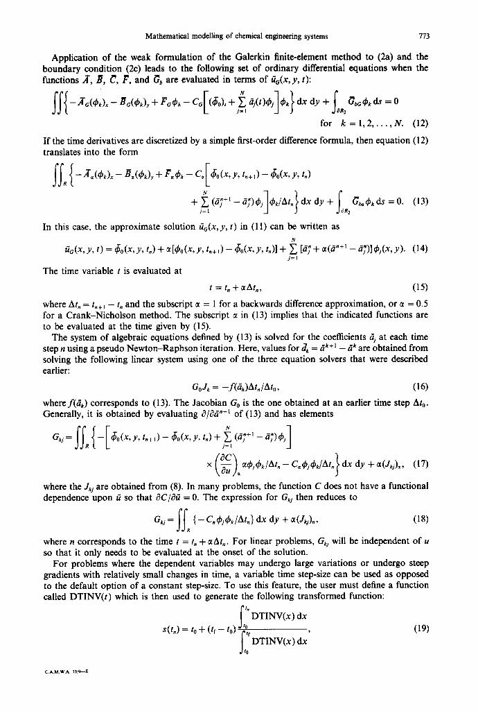
For problems where the dependent variables may undergo large variations or undergo steep gradients with relatively small changes in time, a variable time step-size can be used as opposed to the default option of a constant step-size. To use this feature, the user must define a function called DTINV(t) which is then used to generate the following transformed function:

' [ ' DTINV(x) dx

s(t.) = to + ( t f - to) iilt , (19) DTINV(x) dx

C.A.M.W.A. 15/9---E


where to and tf denote the initial and final values of time. All functions in (13) are then evaluated at the graded values of time t, = t[s(t,) + ~At] where ~ = 1/2 or 1 for the Crank-Nicholson or backwards difference methods, and At is the average step-size. The transformation defined above by (19) provides an array of time base points that allow the use of an optional Richardson's extrapolation to double the order of convergence.

When the time-dependent problem defined by (2a)-(2d) is a hyperbolic system as opposed to a parabolic system, the potential development of discontinuities in the solution may result in spurious or solutions of low accuracy when P D E / P R O T R A N is applied. This is not surprising since it employs a fixed spatial grid and one based upon moving grid has been demonstrated to be superior [26]. By the addition of appropriate terms in the model equations that introduce artificial diffusion, smooth solutions that extend beyond discontinuities can be obtained. The details associated with this procedure and other related aspects are available in Chapter 5 of [41], to which the interested reader is directed.

E X A M P L E A P P L I C A T I O N S OF P D E / P R O T R A N

Several examples that illustrate the use of P D E / P R O T R A N are now introduced to familiarize the reader with translation of typical mathematical modelling equations into a working computer code. While P D E / P R O T R A N has many advanced features, the usage of these here is minimized to avoid possible confusion. Once familiarity with the basic features is mastered, the user can then begin to explore more complex problems where the advanced programming capabilities of P R O T R A N are desirable.

Example 1. Diffusion and reaction in a partially wetted catalyst

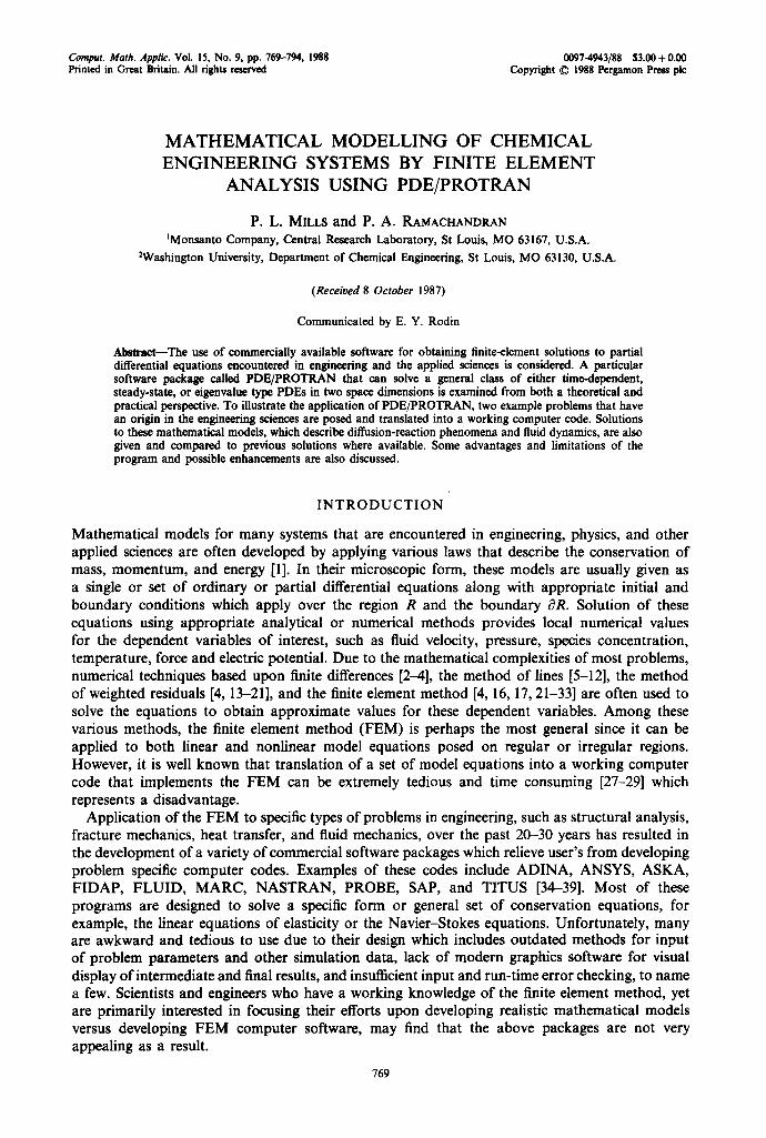
One reactor type that is commonly used in the petroleum and chemical industries to carry out complex reactions at elevated temperature and pressure is the trickle-bed reactor [45]. Here, a gaseous reactant, such as hydrogen, is pumped under pressure to the top of a cylindrical tower where it mixes with a heated flowing liquid stream, such as crude oil. These two streams, which now co-exist as distinct gas-liquid phases, flow under the influence of gravity and pressure differential downward through the tower which is randomly packed with small catalyst pellets. The catalyst pellets, whose diameter is typically 3.2 cm, consist of a porous material, such as ~-alumina with mixed metal oxides, that promote the conversion of sulfur-bearing organic molecules in the crude oil to hydrogen sulfide which is later removed. Due to process constraints and other reasons, the reactors are often operated such that some of the catalyst surfaces are covered by thin, flowing liquid rivulets, while others are covered by stagnant liquid films or exist in direct contact with the gas [46]. To develop accurate predictions of the reactor performance, a mathematical model that describes the effect of catalyst wetting on overall catalyst performance is useful. One model that has been used to perform this task involves a description of diffusion and reaction of the key reactants into the porous catalyst. A detailed derivation of this model is available for several cases of interest [46] so that one of these will be lightly sketched here for clarity in the development that follows.

Referring to Fig. la, a single reaction having the stoichiometry A ( g ) + B( I )~P( I ) is assumed to occur in a catalyst pellet having a rectangular shape whose width and half thickness are w and L respectively. Other more realistic catalyst shapes, such as spheres and cylinders, could be used, but predictions from these are similar to those obtained from the rectangular geometry problem when appropriate shape normalization factors are introduced [46, 49]. Since the rectangular geometry problem posed on Cartesian coordinates is easiest to solve, the choice of this shape is used here. Within the catalyst pellet, the gas A or liquid reactant B is assumed to react according to a power law rate equation of the form R = kC ~ where C = CA is the dissolved gas concentration when the gas is the limiting reactant, or C = Cn is the liquid concentration when the liquid is the limiting reactant. The lower edge of the catalyst y = 0 is assumed to be wetted by actively flowing liquid for 0 ~< x < p , and covered by a stagnant liquid or in direct contact with the gas for p < x ~< w. The line of symmetry is at y = L, while the remaining catalyst surfaces at x = 0 and x = w are impermeable to reactant. With these assumptions, the mass balance equation and


dU - 0

dU - 0 O'q

~'2 u = (b~U (x

i

0 p/w

1 du + u = 1 . 1 Ou BI w o-q Bi d a~

"q

1 . 0

(~U = 0 0.5 1

0.0

I - - - - + U = ~

0.0

$

5

5

2 I

- 2 o r 2 I 3 I I

p/w

4

3

t I

1.0

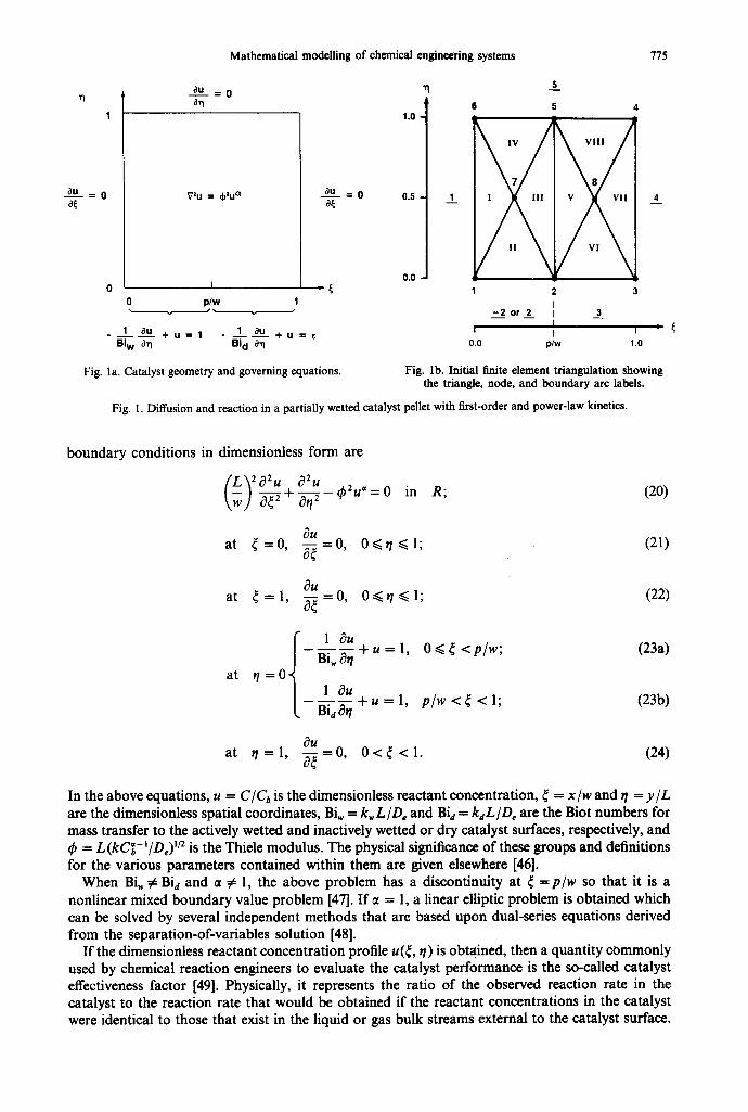
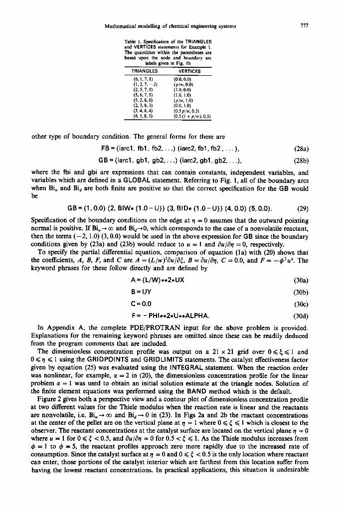
Fig. la. Catalyst geometry and governing equations. Fig. lb. Initial finite element triangulation showing the triangle, node, and boundary arc labels.

Fig. I. Diffusion and reaction in a partially wetted catalyst pellet with first-order and power-law kinetics.

boundary conditions in dimensionless form are

( L V o 2 u ~2u 2 ;) = o in R; (20)

~u at ~ = 0 , - ~ = 0 , O~<r/~<l; (21)

o~

at ¢ = 1 , ~ = 0 , O ~ < n ~ < l ; (22) a~

at f 1 8u

-Bi---Sa---~ + u = 1, 0~<~ <p/w; (23a)

r / = 0 1 au

-- Bi---dd-r~ + u = 1, p/w < ~ < 1; (23b)

~u at ~ = 1, ~ = O, 0 < ~ < 1. (24)

og

In the above equations, u = C/Cb is the dimensionless reactant concentration, ~ = x/w and ~ = y/L are the dimensionless spatial coordinates, Biw = kwL/D~ and Bid = kdL/D~ are the Biot numbers for mass transfer to the actively wetted and inactively wetted or dry catalyst surfaces, respectively, and dp = L (kC~-t/De)I/2 is the Thiele modulus. The physical significance of these groups and definitions for the various parameters contained within them are given elsewhere [46].

When Biw # Bid and ~t # 1, the above problem has a discontinuity at ~ =p/w so that it is a nonlinear mixed boundary value problem [47]. If ~ = 1, a linear elliptic problem is obtained which can be solved by several independent methods that are based upon dual-series equations derived from the separation-of-variables solution [48].

If the dimensionless reactant concentration profile u (~, r/) is obtained, then a quantity commonly used by chemical reaction engineers to evaluate the catalyst performance is the so-called catalyst effectiveness factor [49]. Physically, it represents the ratio of the observed reaction rate in the catalyst to the reaction rate that would be obtained if the reactant concentrations in the catalyst were identical to those that exist in the liquid or gas bulk streams external to the catalyst surface.


It is given by the following quadrature which will be bounded between 0 and 1 for the cases of interest here:

fo'fo' r/rB = U=(~, ~/) d~ d~/. (25)

Thus, the catalyst effectiveness factor is the volume contained beneath the u=(~, r/) surface for 0 ~ < ~ < 1 and 0~r /~< 1.

To solve the above system of equations given by (20)-(24) using PDE/PROTRAN, it is first necessary to develop an initial triangulation that has the simplest possible form without violating certain criteria. These criteria are: (1) at least one of the vertices of a given triangle must be within the interior of R, i.e. a maximum of two vertices of a given triangle can lie on the boundary of R; (2) the intersection of two or more boundary arcs must represent a vertex that is shared by two or more triangular elements; (3) a vertex located within the interior of R must be shared by three or more triangles; and (4) if the segment of a triangle is located on a boundary, it must have a uniform boundary condition applied along this segment or arc.

Figure lb gives the initial triangulation that can be developed when the above rules are applied to the geometry given in Fig. la. Since the boundary condition at t / = 0 has a boundary condition discontinuity at ~ = p/w, a triangle vertex must be placed there so that criterion (4) is not violated. To prevent any violation of the remaining rules, a total of eight triangles must be used for the initial triangulation.

Additional inspection of Fig. lb shows that both the triangles and triangle vertices or nodes are distinctly labeled with integers. The order in which the labels are assigned is arbitrary and left to the discretion of the user, but some consistent procedure is recommended. Here, Roman numerals were assigned to the triangles and Arabic numerals were assigned to the nodes, with both being placed in a counterclockwise rotation for simplicity.

The method used by PDE/PROTRAN to distinguish between the type of boundary condition is based upon the use of signed integers as boundary arc labels. Thus, any boundary arc that has a Dirichlet boundary condition corresponding to equations (lb), (2b), or (3b) must be assigned a negative integer, while any remaining type of boundary conditions, for example, Neumann or Robin types, must be assigned positive integers. In Fig. lb, the boundary arcs are labeled with integers 1-5 which are underlined to avoid possible confusion with the node labels. Thus use of positive integers is consistent with the Neumann and Robin boundary conditions given by (21)-(24). If the mass transfer resistance on the actively wetted surface is negligible, then Bi,--,oo in (23a) so that it reduces to the Dirichlet condition u = 1 and the boundary arc label assumes a value of - 2.

Once the triangles, triangle nodes or vertices, and boundary arcs are appropriately labeled, the user can specify the triangle nodes and vertex coordinates by constructing the T RIANG L ES and VERTICES statements. The general form of the TRIANGLES statement is

TRIANGLES = ( ia l , ib l , ic l , iarcl ) (ia2, ib2 . . . . ), (26)

where ial, ibl , and icl are the three integers which define the triangle nodes for a given triangle and iarcl is the integer that specifies the boundary arc. The integers that specify the triangle nodes must be arranged in the parentheses so that the nodes are defined in a counterclockwise rotation where the last node icl lies within the interior o f R. If the triangle segment formed by connecting the integers ial and ibl does not lie on the boundary, then iarcl = 0 for that triangle. To define the triangle vertices, one simply identifies the (x ,y) coordinates for each vertex or node and arranges these in increasing order through the statement

VERTICES = ( x l , y l ) (x2, y2) . . . (xN, yN). (27)

Table 1 gives a summary of the TRIANGLES and VERTICES statements for this example whose development follows directly from Fig. lb.

Specification of the boundary conditions on each of the boundary arcs is accomplished using the FR keywork phrase for Dirichlet boundary conditions, and the GB keyword phrase for any

Mathemat ica l modell ing o f chemical engineering systems 777

Table 1. Specification of the TRIANGLES and VERTICES statemonts for Example I. The quantitites within the parentheses are based upon the node and boundary arc

labels given in Fig. Ib

TRIANGLES VERTICES

(6, 1,7, 1) (0.0, 0.0) (1, 2, 7, - 2 ) (p/w, 0.0) (2, 5, 7, 0) (1.0, 0.0) (5, 6, 7, 5) (1.0, 1.0) (5, 2, 8, 0) (p/w, 1.0) (2, 3, 8, 3) (0.0, 1.0) (3, 4, 8, 4) (0.5p/w, 0.5) (4, 5, 8, 5) (0.5 (1 + p/w), 0.5)

other type of boundary condition. The general forms for these are

FB = (iarc1, fbl , fb2 . . . . ) (iarc2, fb l , fb2 . . . . ), (28a)

GB = (iarcl, gb l , gb2 . . . . ) (iarc2, gbl , gb2 . . . . ), (28b)

where the fbi and gbi are expressions that can contain constants, independent variables, and variables which are defined in a GLOBAL statement. Referring to Fig. l, all of the boundary arcs when Biw and Bi d a r e both finite are positive so that the correct specification for the G B would be

GB = (1 ,0 .0 ) (2, BIW, (1.0 - U)) (3, BID, ( 1 . 0 - U)) (4, 0.0) (5, 0.0). (29)

Specification of the boundary conditions on the edge at ~/= 0 assumes that the outward pointing normal is positive. If Biw--+ oo and Bid--+0 , which corresponds to the case of a nonvolatile reactant, then the terms ( - 2, 1.0) (3, 0.0) would be used in the above expression for G B since the boundary conditions given by (23a) and (23b) would reduce to u = 1 and c9u/c9~ I = 0, respectively.

To specify the partial differential equation, comparison of equation (la) with (20) shows that the coefficients, A, B, F, and C are A = ( L / w ) : a u / ~ , B = ~u/~tl, C = 0.0, and F = -~b:u =. The keyword phrases for these follow directly and are defined by

A = (L/W) **2, U X (30a)

B = UY (30b)

C = 0.0 (30c)

F = - PHI**2*U**ALPHA. (30d)

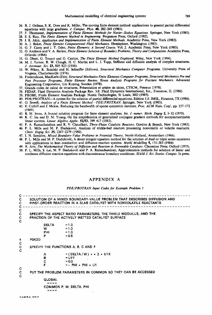
In Appendix A, the complete PDE/PROTRAN input for the above problem is provided. Explanations for the remaining keyword phrases are omitted since these can be readily deduced from the program comments that are included.

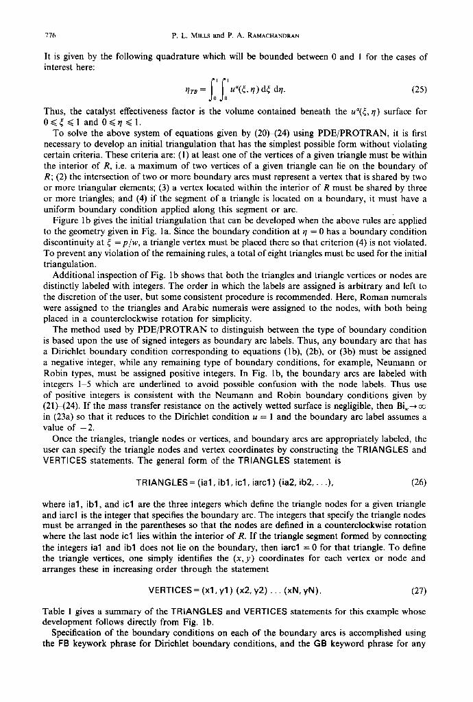
The dimensionless concentration profile was output on a 21 x 21 grid over 0 ~< ~ ~< 1 and 0 ~< r/~< 1 using the G R I O POI NTS and G R I D kl M ITS statements. The catalyst effectiveness factor given by equation (25) was evaluated using the INTEGRAL statement. When the reaction order was nonlinear, for example, = = 2 in (20), the dimensionless concentration profile for the linear problem ~t = 1 was used to obtain an initial solution estimate at the triangle nodes. Solution of the finite element equations was performed using the BAND method which is the default.

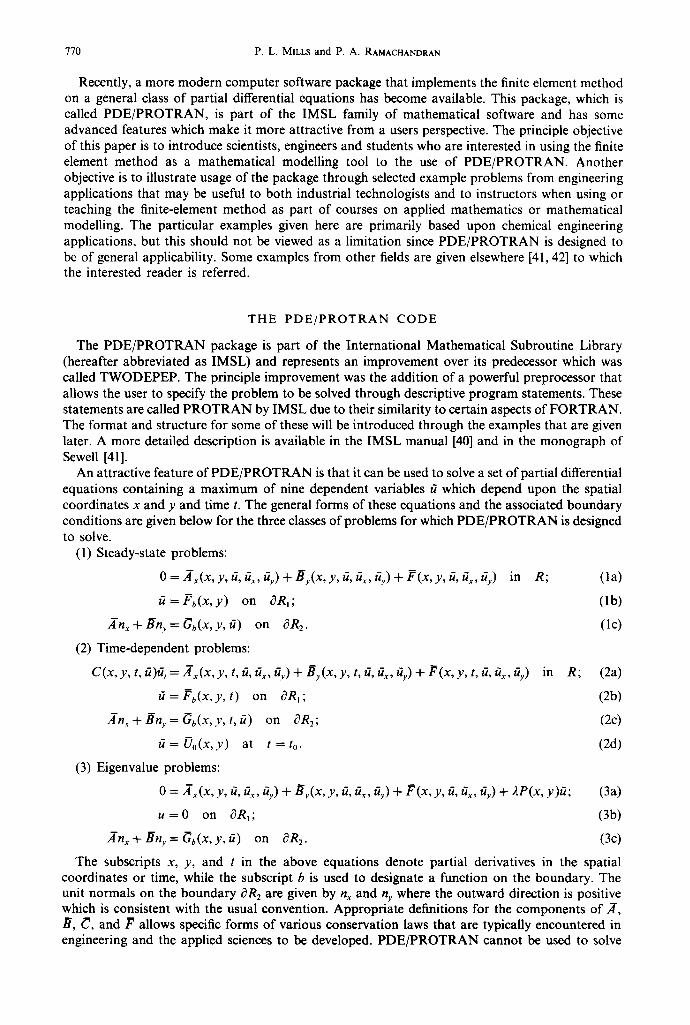
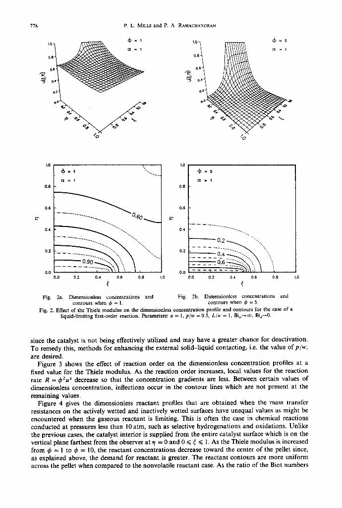
Figure 2 gives both a perspective view and a contour plot of dimensionless concentration profile at two different values for the Thiele modulus when the reaction rate is linear and the reactants are nonvolatile, i.e. Biw--* oo and Bid --* 0 in (23). In Figs 2a and 2b the reactant concentrations at the center of the pellet are on the vertical plane at t / = 1 where 0 ~< ~ ~< 1 which is closest to the observer. The reactant concentrations at the catalyst surface are located on the vertical plane r /= 0 where u = 1 for 0 ~< ~ < 0.5, and ~u/~l = 0 for 0.5 < ~ ~< 1. As the Thiele modulus increases from ~p = 1 to ~b = 5, the reactant profiles approach zero more rapidly due to the increased rate of consumption. Since the catalyst surface at r / = 0 and 0 ~ ~ < 0.5 is the only location where reactant can enter, those portions of the catalyst interior which are farthest from this location suffer from having the lowest reactant concentrations. In practical applications, this situation is undesirable

778 P. L. MILLS and P. A. RAMACHANDRAN

1.0

0.6

c

0.4

0.2

0.0

1.0

0.8

0.6

c

0.4

0.2

0.0

+=5

Q =l

0.0 0.2 0.4 0.6 0.6 1.0 0.0 0.2 0.4 0.6 0.6 I.0

t C

Fig. 2a. Dimensionless concentrations and Fig. 2b. Dimensionless concentrations and contours when I$ = 1. contours when 4 = 5.

Fig. 2. Effect of the Thiele modulus on the dimensionless concentration profile and contours for the case of a liquid-limiting first-order reaction. Parameters: a = 1, p/w = 0.5, L/w = 1, Bi,+a3, B&-+0.

since the catalyst is not being effectively utilized and may have a greater chance for deactivation. To remedy this, methods for enhancing the external solid-liquid contacting, i.e. the value of p/w, are desired.

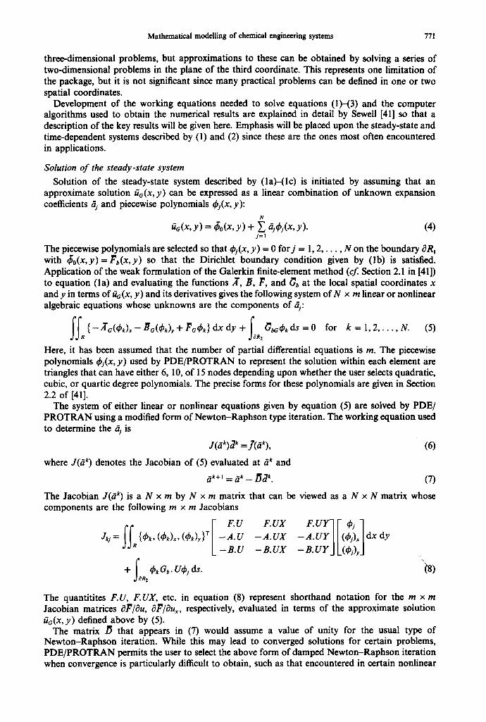
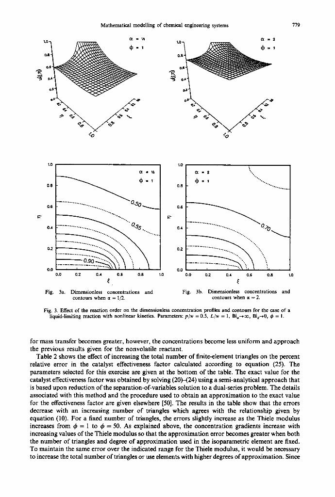
Figure 3 shows the effect of reaction order on the dimensionless concentration profiles at a fixed value for the Thiele modulus. As the reaction order increases, local values for the reaction rate R = c$%P decrease so that the concentration gradients are less. Between certain values of dimensionless concentration, inflections occur in the contour lines which are not present at the remaining values.

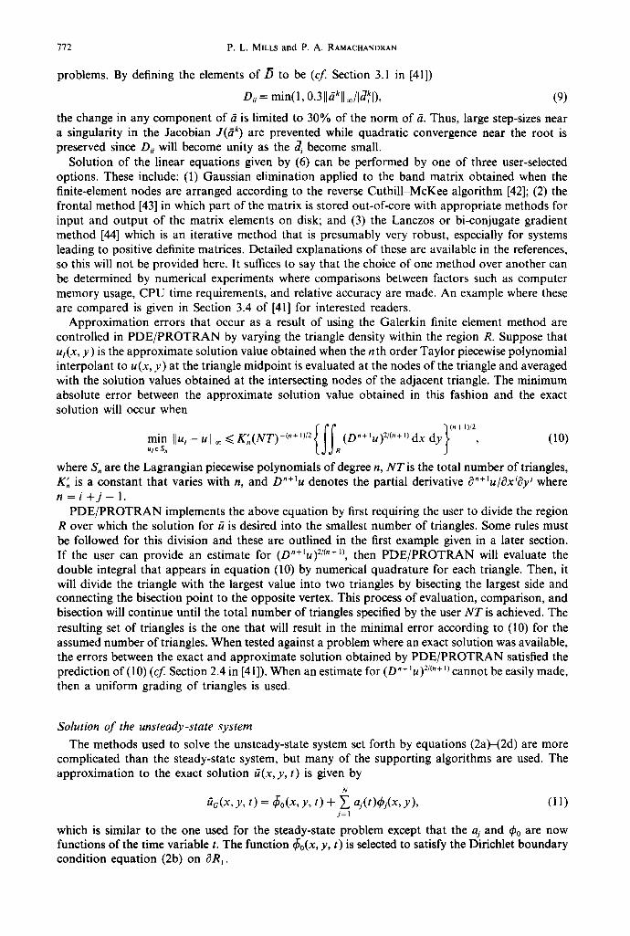
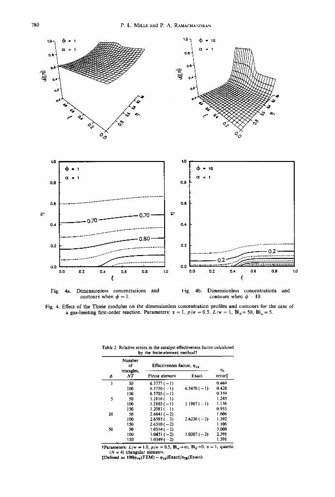
Figure 4 gives the dimensionless reactant profiles that are obtained when the mass transfer resistances on the actively wetted and inactively wetted surfaces have unequal values as might be encountered when the gaseous reactant is limiting. This is often the case in chemical reactions conducted at pressures less than 10 atm, such as selective hydrogenations and oxidations. Unlike the previous cases, the catalyst interior is supplied from the entire catalyst surface which is on the vertical plane farthest from the observer at q = 0 and 0 G 5 < 1. As the Thiele modulus is increased from 4 = 1 to 4 = 10, the reactant concentrations decrease toward the center of the pellet since, as explained above, the demand for reactant is greater. The reactant contours are more uniform across the pellet when compared to the nonvolatile reactant case. As the ratio of the Biot numbers


( ~ , : ½ i v = 2

to ':I) - 1 , , ~ , =

0•6 0•8

0 ~ 0.6

~ o~ -=-~ ,~

• , , ~ o.o ~,~ ~,'~'

• / o e o

K"

1.0 1.0

0 .8

o.6 ............... u"~O ~

0•4

0.0 ' ' 0 .0 0.0 0.2 0.4 0.6 0.8 1.0

Dimensionless concentrations and contours when • = I/2.

t~

0.8

0.8

0.4

0.2

G = 2 \', %,

~°.~o~ 0.0 0.2 0.4 0.6 0.8

Fig. 3a. Fig. 3b.

1.0

Dimensionless concentrations and contours when ~t = 2.

Fig. 3. Effect o f the reaction order on the dimensionless concentration profiles and contours for the case of a liquid-limiting reaction with nonlinear kinetics• Parameters: p/w = 0.5, L/w = 1, Biw--,~, Bid~0, ~b = 1.

for mass transfer becomes greater, however, the concentrations become less uniform and approach the previous results given for the nonvolatile reactant.

Table 2 shows the effect of increasing the total number of finite-element triangles on the percent relative error in the catalyst effectiveness factor calculated according to equation (25). The parameters selected for this exercise are given at the bottom of the table• The exact value for the catalyst effectiveness factor was obtained by solving (20)--(24) using a semi-analytical approach that is based upon reduction of the separation-of-variables solution to a dual-series problem. The details associated with this method and the procedure used to obtain an approximation to the exact value for the effectiveness factor are given elsewhere [50]. The results in the table show that the errors decrease with an increasing number of triangles which agrees with the relationship given by equation (10). For a fixed number of triangles, the errors slightly increase as the Thiele modulus increases from ~b = 1 to $ = 50. As explained above, the concentration gradients increase with increasing values of the Thiele modulus so that the approximation error becomes greater when both the number of triangles and degree of approximation used in the isoparametric element are fixed• To maintain the same error over the indicated range for the Thiele modulus, it would be necessary to increase the total number of triangles or use elements with higher degrees of approximation. Since

780 P . L . MILLS and P. A. RAMACHANDRAN

~.o -.~ ~ = t

Q . 8 ~

0. o ~ " ~ ~ o

o. o

/

0 = 10

O~ = 1 0.8

0.,~'

0.0

o .ox

: 0

g -

1.0 1.0

0.8

0.6

0 . = 1 0.8

0.6 g--

0.4 - - 0 .70 ~ 0.70

0.4

o , . . . . . . .

o.o , S - " ; . . . . . "~ . . . . . , . . . . . 7 . . . . . o .o

o.0 0.2 0.4 0.s 0.a 1.0

0.2

(X = 1

° - " " . . . . . . . . . . . . . . . . . . . . . . . . . . . . .

. . . . . . . . . . . . . . . . . . . . 0 .2

0 .0 0.2 0.4 0.6 0 .8 1.O

Fig. 4a. Dimensionless concentrat ions and Fig. 4b. Dimensionless concentrat ions and contours when ~b = 1. contours when ~b = 10.

Fig. 4. Effect of the Thiele modulus on the dimensionless concentrat ion profiles and contours for the case of a gas-limiting first-order reaction. Parameters: ~ = 1, p / w = 0.5, L / w = I, Bi d = 50, Biw = 5.

Table 2. Relative errors in the catalyst effectiveness factor calculated by the finite-element methodt

Number of Effectiveness factor, r/TS

triangles, % dp N T Finite element Exact error:~

1 50 6.5777 (-- 1) 0.469 100 6.5750 (-- 1) 6.5470 ( - 1) 0.428 150 6.5705 (-- 1) 0.359

5 50 1.2116 ( - l) 1.245 100 1.2103 ( - 1) 1.1967 ( - I ) 1.136 150 1.2081 ( - l) 0.953

20 50 2.6641 ( - 2) 1.606 100 2.6585 ( - 2) 2.6220 ( - 2) 1.392 150 2.6510 ( - 2) 1.106

50 50 1.0514 ( - 2) 3.008 100 1.0451 ( - 2 ) 1.0207 ( - 2 ) 2.391 150 1.0349 ( - 2) 1.391

tParameters: L / w = 1.0, p / w = 0.5, Biw--,co, Bid-~0, " = 1, quartic (N = 4) triangular elements.

:~Defined as 1001~/~(FEM) - I/Ts(Exactl/~TB(Exact).


the indicated errors are satisfactory for engineering applications, the additional computational effort is not justified.

Example 2. Incompressible flow over a step PDE/PROTRAN can be used to solve a wide variety of one- and two-dimensional problems in

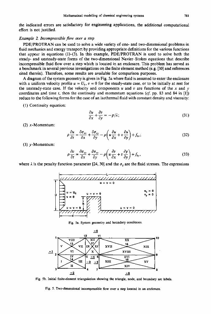
fluid mechanics and energy transport by providing appropriate definitions for the various functions that appear in equations (1)-(3). In this example, PDE/PROTRAN is used to solve both the steady- and unsteady-state forms of the two-dimensional Navier-Stokes equations that describe incompressible fluid flow over a step which is located in an enclosure. This problem has served as a benchmark in several previous investigations on the finite element method (e.g. [30] and references cited therein). Therefore, some results are available for comparison purposes.

A diagram of the system geometry is given in Fig. 5a where fluid is assumed to enter the enclosure with a uniform velocity profile u = U0, v = 0 for the steady-state case, or to be initially at rest for the unsteady-state case. If the velocity and components u and v are functions of the x and y coordinates and time t, then the continuity and momentum equations (cf. pp. 83 and 84 in [1]) reduce to the following forms for the case of an isothermal fluid with constant density and viscosity:

(1) Continuity equation:

(2) x-Momentum:

(3) y-Momentum:

~u ~v +-;- = --p/2; (31)

Ox oy

Ou OOxx OOx, ( Ou Ou) PN = Ox + 7 - f - ° +Ax; (32)

gv dy) +fby, (33) Ov OOxy Oo._p u~+v o N = Ox +-fly

where 2 is the penalty function parameter [24, 30] and the a 0 are the fluid stresses. The expressions

~ L "1 / / / / / / / / / / / / / / / / / / / / / / / / / / / / / / / / / J

u : v : o

_ U x = O Uo . - -v - -o v _ - o l v : ° '

Fig. 5a. System geometry and boundary conditions.

- 1

12 1 10

VIII j

- 8

11 XX \ x I I /

5 - 4

- 3 - 5

-....22 -....s6

Fig. 5b. Initial finite-element triangulation showing the triangle, node, and boundary arc labels.

Fig. 5. Two-dimensional incompressible flow over a step located in an enclosure.


for these latter quantities in terms of the velocity gradients are

axx = 2 ~xx + + 212 ~xx ; (34a)

ayy = 2 0 x x + + 2/2 ~yy, (34b)

axy = # ~xx + " (34c)

The initial and boundary conditions that apply to (31)-(33) are: (i) the fluid is initially at rest for t ~< 0, (ii) a uniform inlet velocity profile for t > 0, and (iii) no fluid slip at all solid walls. The specific ones for the geometry shown in Fig. 5a are summarized below:

at t = 0 , u = v = 0 in R; (35a)

x = o f U =Uo, 0 < y < D ; (35b) at \v = 0 , t >0 ; (35c)

at y = 0 , u = v = 0 , 0 < x < d , ( d + h ) < x < L , t > 0 ; (35d)

at y = h , u = v = 0 , d < x < d + h , t > 0 ; (35e)

at x = d , u = v = 0 , 0 < y < h , t > 0 ; (35f)

at x = d + h , u=v=O, 0 < y < h , t > 0 , (35g)

at y = D , u = v = 0 , 0 < x < L , t > 0 ; (35h)

at x = L , Ux=Vy=O, 0 < y < D , t > 0 . (35i)

Once equations (31)-(35) are solved, approximate values for the fluid pressure at (x,y) can be obtained by combining equations (31), (34a) and (34b) to yield

2((Txx .31- ayy) (36) P = P 0 2 ( 2 + p ) '

where P0 is a reference pressure at some reference coordinate (x0, Y0)- The choice of the penalty 2 that appears in the above equations is discussed in detail by Baker

[30]. An approximate criteria is that 2 = C max(v, vRe) where v = g/p is the kinematic viscosity, Re is the Reynolds number, and C is a constant. For the results presented here, it was determined by numerical experiments that convergence could be obtained by choosing 2 = 106-108 when the calculations were performed in double precision on an IBM 3083 (about 12-14 digits). If other problems are attempted, or another computer that carries a different number of digits is used, then use of another value for 2 may be necessary. Proper choice of the penalty function parameter will ensure that the continuity equation given by equation (34) will be automatically satisfied with an absolute value for the error of p/2 plus rounding errors once approximate values for the velocity vector components {u, v } have been obtained that satisfy the momentum equations at each of the element nodes.

Development of a P D E / P R O T R A N input code for this example is similar to that described in the previous example, except that there are now two unknowns {u, v} as opposed to one and the partial differential equations have stronger nonlinearities. Specification of the coefficients ,,T, B, •, and b" can be readily performed by comparison of equation (2a) to (32) and (33). This shows that

iT = (axx, trxy); (37a)

B = (axy, ayy); (37b)

~' = (p, p); (37c)

F = [-p(uux + vuy), -p(uv~ + VVy)], (37d)

where the body forces fox and foy in F are assumed to be negligible. The steady-state problem is obtained by defining ~' = {0.0, 0.0} since u, = vt = 0 in equations (32) and (33), respectively.

Mathema t i ca l model l ing o f chemical engineer ing sys tems 783

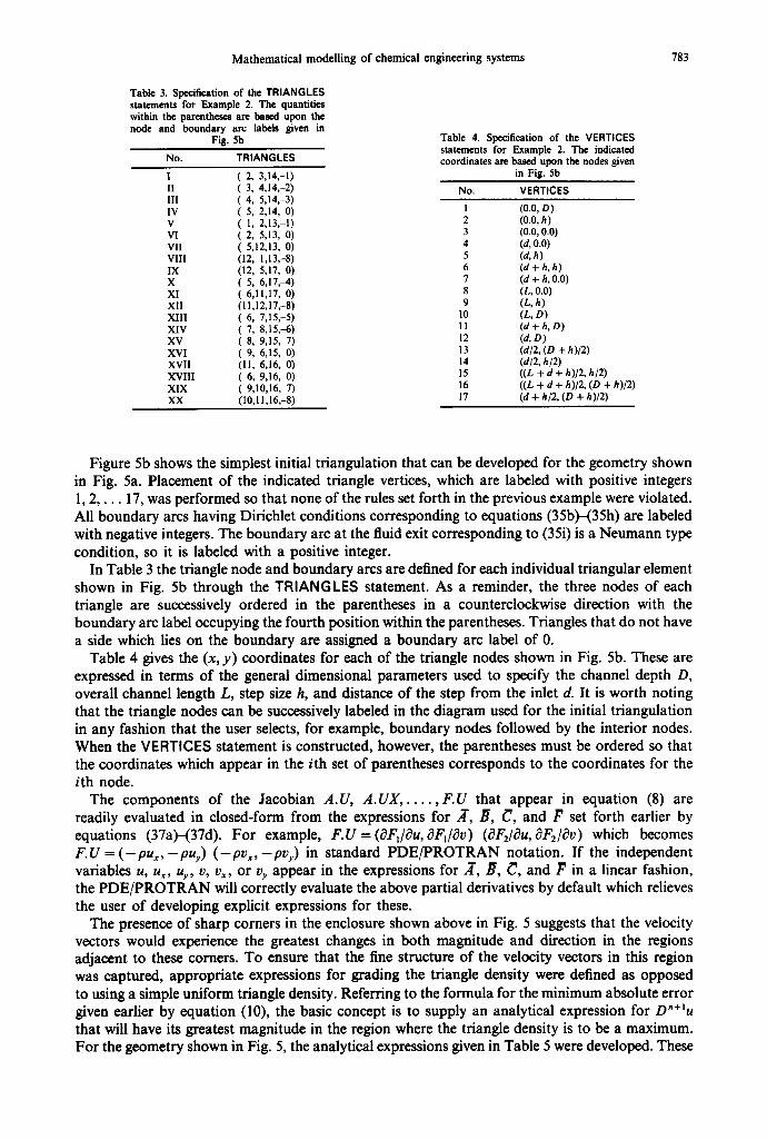
Table 3. Specification of the TRIANGLES smt~ 'n~ts for Example 2. The quantities within the parentheses are based upon the node and boundary arc labels given in

Fig. 5b Table 4. Specification of the VERTICES statements for Example 2. The indicated

No. TRIANGLES coordinates are based upon the nodes given I ( 2, 3,14,-1) in Fig. 5b I I ( 3, 4,14,-2) No. VERTICES III ( 4, 5,14,-3) IV ( 5, 2,14, 0) 1 (0.0, D) V ( 1, 2,13,-I) 2 (0.0, h) VI ( 2, 5,13, 0) 3 (0.0,0.0) VII ( 5,12,13, 0) 4 (d, 0.0) VIII (12, 1,13,-8) 5 (d, h) IX (12, 5,17, 0) 6 (d+h,h) X ( 5, 6,17,4) 7 (d+h,O.O) XI ( 6,11,17, 0) 8 (L,0.0) XII (11,12,17,-8) 9 (L, h) XIII ( 6, 7,15,-5) 10 (L, D) XIV ( 7, 8,15,-6) 11 (d+h,D) XV ( 8, 9,15, 7) 12 (d,O) XVI ( 9, 6,15, 0) 13 (d/2, (D + h)/2) XVII (1 l, 6,16, 0) 14 (d/2, hi2) XVIII ( 6, 9,16, 0) 15 ((L + d + h)/2, h/2) XIX ( 9,10,16, 7) 16 ((L + d + h)/2, (D + h)/2) XX (10,11,16,--8) 17 (d + h/2, (D + h)/2)

Figure 5b shows the simplest initial triangulation that can be developed for the geometry shown in Fig. 5a. Placement of the indicated triangle vertices, which are labeled with positive integers 1, 2 . . . . 17, was performed so that none of the rules set forth in the previous example were violated. All boundary arcs having Dirichlet conditions corresponding to equations (35b)-(35h) are labeled with negative integers. The boundary arc at the fluid exit corresponding to (35i) is a Neumann type condition, so it is labeled with a positive integer.

In Table 3 the triangle node and boundary arcs are defined for each individual triangular element shown in Fig. 5b through the TRIANGLES statement. As a reminder, the three nodes of each triangle are successively ordered in the parentheses in a counterclockwise direction with the boundary arc label occupying the fourth position within the parentheses. Triangles that do not have a side which lies on the boundary are assigned a boundary arc label of 0.

Table 4 gives the (x, y) coordinates for each of the triangle nodes shown in Fig. 5b. These are expressed in terms of the general dimensional parameters used to specify the channel depth D, overall channel length L, step size h, and distance of the step from the inlet d. It is worth noting that the triangle nodes can be successively labeled in the diagram used for the initial triangulation in any fashion that the user selects, for example, boundary nodes followed by the interior nodes. When the VERTICES statement is constructed, however, the parentheses must be ordered so that the coordinates which appear in the ith set of parentheses corresponds to the coordinates for the ith node.

The components of the Jacobian A.U, A . U X . . . . . . F.U that appear in equation (8) are readily evaluated in closed-form from the expressions for ~T, •, C, and F set forth earlier by equations (37a)-(37d). For example, F.U = (OF,/au, OFl/av) (OFE/OU, OF2/Ov) which becomes F.U = ( - p u x , - p U y ) ( - p v , , , - p r y ) in standard PDE/PROTRAN notation. If the independent variables u, ux, uy, v, vx, or vy appear in the expressions for/T, J~, C, and P in a linear fashion, the PDE/PROTRAN will correctly evaluate the above partial derivatives by default which relieves the user of developing explicit expressions for these.

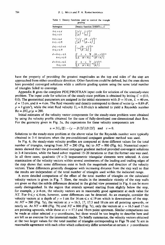
The presence of sharp comers in the enclosure shown above in Fig. 5 suggests that the velocity vectors would experience the greatest changes in both magnitude and direction in the regions adjacent to these comers. To ensure that the fine structure of the velocity vectors in this region was captured, appropriate expressions for grading the triangle density were defined as opposed to using a simple uniform triangle density. Referring to the formula for the minimum absolute error given earlier by equation (10), the basic concept is to supply an analytical expression for D"+tu that will have its greatest magnitude in the region where the triangle density is to be a maximum. For the geometry shown in Fig. 5, the analytical expressions given in Table 5 were developed. These

784 P. L. MILLS and P. A. RAMACHANDRAN

Table 5. Density functions used to control the triangle grading

Subregion Density function D3EST(x,y)

[(0 (Y)T O<~y<~h ~1 +

O<<.x<~d I(x) 2 (D - y)2] ',2 h < . y < O 2 +

h < ~ y ~ O L - ( d + h ) +

0~,.~<h L - -?d~h)j +

have the property of providing the greatest magnitudes as the top and sides of the step are approached from either coordinate direction. Other functions could be defined, but the ones shown here provided converged solutions while a uniform grading system using the same total number of triangles failed to converge.

Appendix B gives the complete P D E / P R O T R A N input code for solution of the unsteady-state problem. The input code for solution of the steady-state problem is obtained by letting C = (0.0, 0.0). The geometrical parameters are assigned in the initial statements with D = 10 cm, L = 40 cm, d = 12 cm, and h = 4 cm. The fluid viscosity and density correspond to those of water (/~ = 0.89 cP, p = 1 g/cm3), while the inlet fluid velocity U0 = 0.18 cm/s is selected to yield a Reynolds number Re = D U0 p/# = 200.

Initial estimates of the velocity vector components for the steady-state problem were obtained by using the velocity profile obtained for the case of fully-developed one-dimensional duct flow. For the geometry given in Fig. 5a, the expressions for these velocity components are

u = 3U0/2[1 -- (y -- D /2 )2 / (D/2 ) 2] and v = 0.

Solutions to the steady-state problem at the above value for the Reynolds number were typically obtained in 3--4 iterations when the pre-conditioned conjugate gradient method was used.

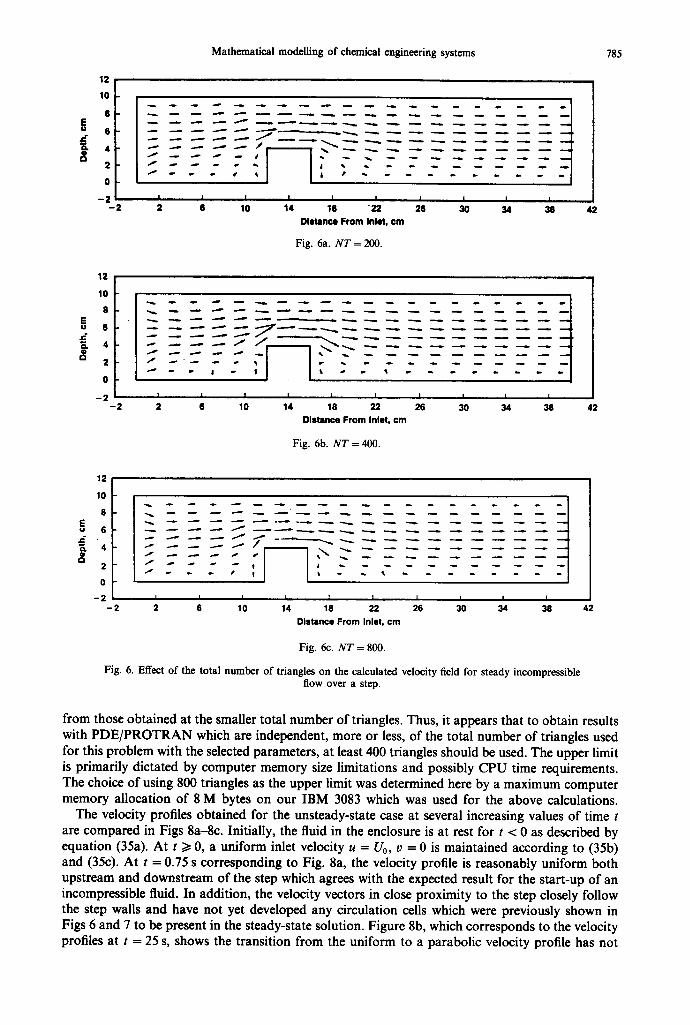
In Fig. 6, the steady-state velocity profiles are compared at three different values for the total number of triangles, ranging from N T = 200 (Fig. 6a) to N T = 800 (Fig. 6c). Numerical experiments showed that the pre-conditioned conjugate gradient method provided convergent solutions in 3-4 iterations, while the band solver required 15-20 iterations so that the former one was used. In all three cases, quadratic (N = 2) isoparametric triangular elements were selected. A close examination of the velocity vectors within several centimeters of the leading and trailing edges of the step shows that some differences exist in both the magnitude and direction of the velocity vectors. These differences generally disappear with increasing distance from the step wall so that the results are independent of the total number of triangles used within the indicated range.

A more detailed comparison of the effect of the total number of triangles on the calculated velocity vectors is given in Fig. 7. Here, the results in the immediate vicinity of the step walls are given so that the subtle differences detected in the global view presented in Fig. 6 can be more easily distinguished. In the region that extends upward starting from slightly below the step, for example, y /> 4 cm, the velocity vectors are in reasonably good agreement at each value for N T . For 0 ~< y ~< 4 cm, however, some differences can be detected. As an example, consider the velocity vectors at a depth of y = 1 cm for 16 cm ~< x ~< 19 ern which is downstream of the step. At N T = 200 (Fig. 7a), the vectors at x = 16.5, 17, 17.5 and 18 cm are all pointing upwards, or nearly so. At N T = 400 (Fig. 7b) and N T = 800 (Fig. 7c), only the vectors at x = 16.5 and 17 cm are pointing upwards, while those at x = 17.5 and 18 cm point upstream. Similar comparisons can be made at other selected x - y coordinates, but these would be too lengthy to describe here and are left as an exercise for the interested reader. To briefly summarize, the velocity vectors obtained at the two larger values for the total number of triangles corresponding to Figs 7b and 7c are in reasonable agreement with each other which collectively differ somewhat at certain x - y coordinates


12

E f J

J : : K

lO

8

6

4

2

0

- 2 - 2

. . ,4" :] I I I I ! I I I

2 6 10 14 111 "22 26 30 Distance From Inlet, cm

Fig. 6a. N T = 200.

I I 34 38 42

12

6 q

4

0

- 2 I - 2 2 6 10 14 111 22 26 30 34 38 42

Distance From Inlet, cm

Fig. 6b. N T = 400.

E

12

10

8

6

4 "~" J

2 f

0 - 2 I

- 2 2

~ ..... ~ i --'-"--~ ~

I I I I I I I I I

6 10 14 18 22 26 30 34 38


42

Fig. 6c. N T = 800.

Fig. 6. Effect of the total number of triangles on the calculated velocity field for steady incompressible flow over a step.

from those obtained at the smaller total number of triangles. Thus, it appears that to obtain results with PDE/PROTRAN which are independent, more or less, of the total number of triangles used for this problem with the selected parameters, at least 400 triangles should be used. The upper limit is primarily dictated by computer memory size limitations and possibly CPU time requirements. The choice of using 800 triangles as the upper limit was determined here by a maximum computer memory allocation of 8 M bytes on our IBM 3083 which was used for the above calculations.

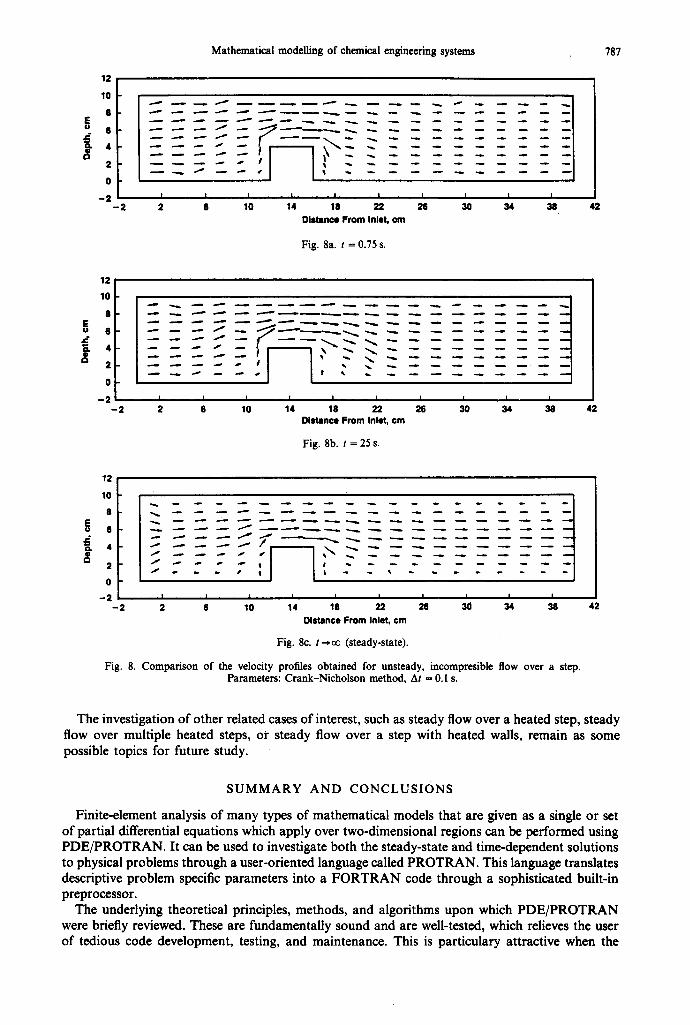
The velocity profiles obtained for the unsteady-state case at several increasing values of time t are compared in Figs 8a-8c. Initially, the fluid in the enclosure is at rest for t < 0 as described by equation (35a). At t /> 0, a uniform inlet velocity u = U0, v = 0 is maintained according to (35b) and (35c). At t = 0.75 s corresponding to Fig. 8a, the velocity profile is reasonably uniform both upstream and downstream of the step which agrees with the expected result for the start-up of an incompressible fluid. In addition, the velocity vectors in close proximity to the step closely follow the step walls and have not yet developed any circulation cells which were previously shown in Figs 6 and 7 to be present in the steady-state solution. Figure 8b, which corresponds to the velocity profiles at t = 25 s, shows the transition from the uniform to a parabolic velocity profile has not


- - # # O S ,

. . . . . .

. . . . , t

i . . . . . i

3

I

- - I 9 I 0 I

I h * L ' '

I * . . . .

i i i i

1 2 1 3 1 4 1 5

Distance From InLet, cm

Fig. 7a. N T = 200.

2o

3

~ 2

~ p p - - , ,

- - , , ~ t

- , ~ t a ,

i , . . . .

L , . . . .

Distance From InLet, cm

Fig. 7b. N T = 400 .

20

6 ,

E o 3

h /

. . . . , f

. . . . p *

, . ° . , ,

• , , . . .

Distance From InLet~ cm

Fig. 7c. N T = 800.

Fig. 7. Expanded view of the velocity vectors in close proximity to the step showing the effect of the total number of triangles.

yet occurred when compared to the steady-state solution in Fig. 8c. However, the velocity profile downstream of the step corresponding to 16 < x < 22 cm has changed noticeably from the one obtained earlier at t = 0.75 s shown in Fig. 8a. Calculations for larger values of time which show the full development of the parabolic velocity profile were not performed since the objective here was to briefly demonstrate the solution at smaller values of time t where the CPU time was not excessive,

--L 787 Mathematical modelling o f chemical engineering systems

12

10

i 6 i - -

2

0

- 2 I I I i I - 2 2 6 10 14 18 22 26 30 34 38


Fig. 8a. t = 0.75 s.

42

--t I

12

", "1 I' "

- 2 I I I I i - 2 2 6 10 14 18 22 26 30


Fig. 8b. t = 25 s.

I 34 38 42

J= D.

12

10

8

6

4

2

0

- 2

I L, I i i i I i i i I I 2 6 10 14 18 22 26 30 34 38

Ohltance From Inlet, cm

Fig. 8c. t-~oo (steady-state).

Fig. 8. Compar ison o f the velocity profiles obtained for unsteady, incompresible flow over a step. Parameters: Crank-Nicholson method, At = 0.1 s.

42

The investigation of other related cases of interest, such as steady flow over a heated step, steady flow over multiple heated steps, or steady flow over a step with heated walls, remain as some possible topics for future study.

SUMMARY AND CONCLUSIONS

Finite-element analysis of many types of mathematical models that are given as a single or set of partial differential equations which apply over two-dimeusional regions can be performed using PDE/PROTRAN. It can be used to investigate both the steady-state and time-dependent solutions to physical problems through a user-oriented language called PROTRAN. This language translates descriptive problem specific parameters into a FORTRAN code through a sophisticated built-in preprocessor.

The underlying theoretical principles, methods, and algorithms upon which PDE/PROTRAN were briefly reviewed. These are fundamentally sound and are well-tested, which relieves the user of tedious code development, testing, and maintenance. This is particulary attractive when the


applications encountered by the user are varied and minimal time is available for obtaining a solution. In addition, students of applied mathematics and engineering, once familiarized with the basics of the finite-element method, can readily use PDE/PROTRAN through problem solving to reinforce these basic concepts.

PDE/PROTRAN is not specifically designed to solve mathematical models involving free surfaces or other related problems where one or more of the boundaries are not known or fixed a priori . In addition, solutions to problems posed in three spatial dimensions cannot be developed since PDE/PROTRAN is limited to two spatial dimensions and time. This limitation is not particularly severe since most physical problems can be adequately approximated in two space dimensions. Finally, use of PDE/PROTRAN to investigate bifurcation phenomena has also not been demonstrated. This is a possible topic for future study.

The example problems considered in this work have demonstrated that PDE/PROTRAN is capable of providing reliable finite-element solutions with a minimum of effort on the part of the user. Various other problems, which are too numerous to describe here, have also been successfully solved with this package which supports its utility as a useful piece of numerical software for mathematical modelling. Comparisons between numerical results obtained by PDE/PROTRAN for the example problems to those obtained by other independent methods, where available, showed good agreement. Additional testing of PDE/PROTRAN on application problems and direct comparison of performance to other software packages would be useful information.

R E F E R E N C E S

1. R. B. Bird, W. E. Stewart and E. N. Lightfoot, Transport Phenomena. Wiley, New York (1960). 2. J. Isenberg and G. de Vahl Davis, in Topics in Transport Phenomena (Edited by G. Gutfinger), pp. 457 553. Hemisphere,

New York (1975). 3. A. R. Mitchell and D. F. Griffiths, The Finite Difference Method in Partial Differential Equations. Wiley-Interscience,

New York (1980). 4. B. A. Finlayson, Nonlinear Analysis in Chemical Engineering. McGraw-Hill, New York (1980). 5. O. A. Liskovets, The method of lines (review). Diffl Eqns 1, 1308-1323 (1965). 6. A. F. Cardenas and W. J. Karplus, PDEL--A language for partial differential equations. Commun. ACM 13(3), 184-191

(1970). 7. M. G. Zellner, DSS---distributed system simulator. Ph.D. Thesis, Lehigh University, Bethlehem, PA (1970). 8. M. R. Carver, FORSIM: A FORTRAN oriented simulation package for the automated solution of partial and ordinary

differential equation systems. Report AECL-4608, Atomic Energy of Canada, Limited, Chalk River, Ontario (1973). 9. N. K. Madsen and R. F. Sincovec, PDEPACK: A new tool for simulation. Proc. 1975 Summer Computer Simulation

Conf., San Francisco, CA (1975). 10. R. F. Sincovec and N. K. Madsen, Software for nonlinear partial differential equations. ACM Trans. math. Software

I(3), 232-260 (1975). 1 I. N. K. Madsen and R. F. Sincovec, General software for partial differential equations. In Numerical Methods for

Differential Systems (Edited by L. Lapidus and W. E. Schiesser), pp. 229-242. Academic Press, New York (1976). 12. M. Bieterman and I. Babu~ka, An adaptive method of lines with error control for parabolic equations of the

reaction-diffusion type. Laboratory for Numerical Analysis Technical Note BN-1023, University of Maryland, College Park, MD (1984).

13. B. A. Finlayson, The Method of Weighted Residuals and Variational Principles. Academic Press, New York (1972). 14. J. Villadsen and M. L. Michelsen, Solution of Differential Equations by Polynomial Approximation. Prentice-Hall, New

York (1978). 15. M. A. Neira and A. C. Payatakes, Collocation solution of creeping Newtonian flow through periodically constricted

tubes with piecewise continuous wall profile. AIChE J. 24(1), 43-54 (1978). 16. P. W. Chang, T. W. Patten and B. A. Finlayson, Collocation and Galerkin finite element methods for viscoelastic fluid

flow--I. Description of methods and problems with fixed geometry. Comput. Fluids 7, 267-283 (1979). 17. P. W. Chang, T. W. Patten and B. A. Finlayson, Collocation and Galerkin finite element methods for viscoelastic fluid

flow--II. Die swell problems with a free surface. Comput. Fluids 7, 285-293 (1979). 18. N. K. Madsen and R. F. Sincovec, PDECOL--General collocation software for partial differential equations.

ACM Trans. math. Software 5(3), 326-351 (1979). 19. H. H. Klein, Computer modeling of chemical process reactors. 1st Engineering Conf. Chemical Reaction Engineering,

Miramar Hotel, Santa Barbara, CA (1985). 20. U. Ascher, J. Christiansen and R. D. Russell, Collocation software for boundary-values ODEs. ACM Trans. math.

Software 7(2), 202-222 (1981). 21. L. Lapidus and G. F. Pinder, Numerical Solution of Partial Differential Equations in Science and Engineering.

Wiley-Interscience, New York (1982). 22. H. C. Martin and G. F. Carey, Introduction to Finite Element Analysis. McGraw-Hill, New York (1973). 23. C. Taylor and P. Hood, A numerical solution of the Navier-Stokes equations using the finite element technique.

Comput. Fluids 1, 73-100 (1973). 24. O. C. Zienkiewicz, The Finite Element Method, 3rd edn. McGraw-Hill, New York (1977). 25. A. Trotta and S. D. Giudiee, A finite element solution of coupled heat and mass transfer with chemical reaction.

Chem. Engng Sci. 35, 706-716 (1980).


26. R. J. Gelinas, S. K. Doss and K. Miller, The moving finite element method: applications to general partial differential equations with large gradients. J. Comput. Phys. 40, 202-249 (1981).

27. F. Thomasset, Implementation of Finite Element Methods for Navier-Stokes Equations. Springer, New York (1981). 28. S. S. Rao, The Finite Element Method in Engineering. Pergamon Press, Oxford (1982). 29. J. E. Akin, Application and Implementation of Finite Element Methods. Academic Press, New York (1982). 30. A. J. Baker, Finite Element Computational Fluid Mechanics. Hemisphere, Washington (1983). 31. G. F. Carey and J. T. Oden, Finite Elements: A Second Course, Vol. 2. Academic Press, New York (1983). 32. O. Axelsson and V. A. Barker, Finite Element Solution of Boundary Problems, Theory and Computation. Academic Press,

Orlando (1984). 33. G. Dhatt, G. Touzot and G. Canton, The Finite Element Method Displayed. Wiley, New York (1984). 34. M. J. Turner, R. W. Clough, H. C. Martin and L. J. Topp, Stiffness and diffusion analysis of complex structures.

J. Aeronaut. Sci. 23, 805-823 (1956). 35. W. Pilkey, K. Sczalski and H. Schaeffer (Editors), Structural Mechanics Computer Programs. University Press of

Virginia, Charlottesville (1974). 36. Frederickson, MacKerle (Eds), Structural Mechanics Finite Elements Computer Programs, Structural Mechanics Pre and

Post Processor Programs, Finite Element Review, Stress Analysis Programs for Fracture Mechanics. Advanced Engineering Corporation, Lin Koping, Sweden (1978).

37. Grands codes de calcul de structures, Pr6sentation et crit6re de choix, CTICM, Puteaux (1978). 38. FIDAP, Fluid Dynamics Analysis Package Rev. 3.0. Fluid Dynamics International, Inc., Evanston, IL (1986). 39. PROBE, Finite Element Analysis Package. Noetic Technologies, St Louis, MO (1985). 40. PDE/PROTRAN--A system for the solution of partial differential equations, Edition 1.0. IMSL, Houston, TX (1986). 41. G. Sewell, Analysis of a Finite Element Method--PDE/PROTRAN. Springer, New York (1985). 42. E. Cuthill and J. Mckc¢, Reducing the bandwidth of sparse symmetric matrices. Proc. ACM Natn. Conf., pp. 157-172

(1969). 43. B. M. Irons, A frontal solution program for finite element analyses. Int. J. numer. Meth. Engng 2, 5-32 (1970). 44. K. C. Jea and D. M. Young, On the simplification of generalized conjugate gradient methods for nonsymmetrizable

linear systems. Linear Algebra Applic. 52/53, 399-417 (1983). 45. P. A. Ramachandran and R. V. Chaudhari, Three-Phase Catalytic Reactors. Gordon & Breach, New York (1983). 46. P. L. Mills and M. P. Dudukovi~, Analysis of trickle-bed reactors processing nonvolatile or volatile reactants.

Chem. Engng Sci. 35, 2267-2279 (1980). 47. I. N. Sneddon, Mixed Boandary-Value Problems in Potential Theory. North-HoUand, Amsterdam (1966). 48. P. L. Mills and M. P. Dudukovi~, A direct integral equation method for the solution of dual or triple series equations

with applications to heat conduction and diffusion-reaction systems. Mathl Modelling 5, 171-203 (1984). 49. R. Aris, The Mathematical Theory of Diffusion and Reaction in Permeable Catalysts. Clarendon Press, Oxford (1975). 50. P. L. Mills, S. Lai, M. P. Dudukovi~ and P. A. Ramachandran, Approximation methods for solution of linear and

nonlinear diffusion reaction equations with discontinuous boundary conditions. SIAM J. Sci. Statist. Comput. In press.

C - -

C C C . . . . . . . .

A P P E N D I X A

PDE/PROTRAN Input Codes for Example Problem I

. . . . . . . . . . . . . . . . . . . . . . .

SOLUTION OF A MIXED BOUNDARY-VALUE PROBLEM THAT DESCRIBES DIFFUSION AND FIRST-ORDER REACTION IN A SLAB CATALYST WITH NONVOLATILE REACTANTS

C C C C

$ C C C

C C C

SPECIFY THE ASPECT RATIO PARAMETERS, THE THIELE MODULUS, AND THE FRACTION OF THE ACTIVELY WETTED CATALYST SURFACE

DELTA = 1.0 W = 1.0 PHI = 1.0 P =0.5

PDE2D

SPECIFY THE FUNCTIONS A, B, C AND F

A = ( D E L T A / W ) * * 2 * U1X B = U l Y C =0.0 F = - PHI * PHI * U1

PUT THE PROBLEM PARAMETERS IN COMMON SO THEY CAN BE ACCESSED

GLOBAL

COMMON P, W, DELTA, PHI

C.A.M.W.A. 15/9---F

790 P .L . MILLS and P. A. RAMACI-IANDRAN

C C C

C C C C

C C C C

SPECIFY THE X AND Y COORDINATES OF THE INITIAL TRIANGLE VERTICES

& &

VERTICES = (0.0,0.0) (P/W,0.0) (1.0,0.0) (1.0,1.0) (P/W,1.0) (0.0,1.0) (0.5*P/W,0.5) (0.5.(1.0 + P/W),0.5)

SPECIFY THE INITIAL TRIANGLES ACCORDING TO THE VERTEX INTEGERS AND ARC NUMBERS

& TRIANGLES = (6,1,7,1) (1,2,7,-2) (2,5,7,0) (5,6,7,5)

(5,2,8,0) (2,3,8,3) (3,4,8,4) (4,5,8,5)

SPECIFY THE BOUNDARY CONDITIONS ON EACH BOUNDARY ARC

GB = (1,0.0) (3,0.0) (4,0.0) (5,0.0) FB = (-2,1.0)

SPECIFY THE NUMBER OF TRIANGLES IN THE FINAL MESH, THE METHOD USED TO SOLVE THE FEM EQUATIONS, THE DEGREE OF ISOPARAMETRIC ELEMENT, AND THE MAXIMUM NUMBER OF ITERATIONS

NTRIANGLES = 50 BAND DEGREE = 4 MAXITERATIONS = 25

SPECIFY THE NUMBER OF X AND Y GRIDPOINTS AT WHICH THE SOLUTION WILL BE INTERPOLATED AND THE OUTPUT FILE NAME

GRIDPOINTS = (21, 21) GRIDLIMITS = ( 0., 1.0) (0., 1.0) SAVEFILE = PLOT

EVALUATE THE EFFECTIVENESS FACTOR BY INTEGRATING THE CONCENTRATION PROFILE OVER THE REGION R

$ END INTEGRAL = U1

C ...........................................................

C C C . . . . . . . .

C

C

C

C

SOLUTION OF A MIXED BOUNDARY-VALUE PROBLEM THAT DESCRIBES DIFFUSION AND NTH-ORDER REACTION IN A SLAB CATALYST WITH NONVOLATILE REACTANTS

. . . . . . . . . . . . . . . . . . . . . . . . . . . . . . . . . . . . . . . . . . . . . . . . . . .

SPECIFY THE ASPECT RATIO PARAMETERS, THE THIELE MODULUS, THE FRACTION OF THE CATALYST SURFACE THAT IS ACTIVELY WETTED, AND THE REACTION ORDER

DELTA = 1.0 W = 1.0 PHI = 5.0 P =2.0

PDE2D

SPECIFY THE DEPENDENT VARIABLE NAME

UNKNOWNS = U

SPECIFY THE FUNCTIONS A, B, C, AND F

A = ( D E L T A / W ) * * 2 * UX B = UY C =0.0 F = - PHI * PHI * U ** ORDER

SPECIFY THE REACTION ORDER

DEFINE

IF (T .LE. 1.0) THEN ORDER = 1.0 ELSE ORDER =2.0 END IF

C C C

C C C

C C C

C C C

Mathematical modelling of chemical engineering systems

SPECIFY THE JACOBIAN OF F, I.E., DF/DU

F.U =-ORDER • PHI • PHI • U ** (ORDER- 1.0)

PUT THE PROBLEM PARAMETERS IN COMMON SO THAT THEY CAN BE ACCESSED

GLOBAL = m m m

COMMON P , W , DELTA , PHI , ORDER

SPECIFY THE X AND Y COORDINATES OF THE INITIAL TRIANGLE VERTICES

VERTICES = (0.0,0.0) (P/W,0.0) (1.0,0.0) (1.0,1.0) & (P/W,1.0) (0.0,1.0) (0.5.P/W,0.5) & (0.5.(1.0+ P/W),0.5)

SPECIFY THE INTEGERS USED TO IDENTIFY THE TRIANGLE VERTICES

TRIANGLES = (6,1,7,1) (1,2,7,-2) (2,5,7,0) (5,6,7,5) & (5,2,8,0) (2,3,8,3) (3,4,8,4) (4,5,8,5)

SPECIFY THE BOUNDARY CONDITIONS ON EACH ARC

GB = (1,0.0) (3,0.0) (4,0.0) (5,0.0) FB = (-2,1.0)

SPECIFY AN INITIAL ESTIMATE OF THE CONCENTRATION PROFILE

U0 =P/W • COSH( PHI • ( 1 . - Y ) ) / COSH ( PHI )

SPECIFY THAT THE JACOBIAN ASSOCIATED WITH THE FUNCTIONS A, B, C AND F IS SYMMETRIC

SYMMETRIC

SPECIFY THE NUMBER OF TRIANGLES DESIRED IN THE FINAL TRIANGULATION AND THE MAXIMUM NUMBER OF ITERATIONS

NTRIANGLES = 200 MAXITERATIONS = 25 STEPLIMIT

SPECIFY THE NUMBER OF X AND Y GRIDPOINTS AT WHICH THE SOLUTION WILL BE EVALUATED AND THE X AND Y COORDINATE LIMITS

GRIDPOINTS = (21, 21 ) GRIDLIMITS = (0 .0 , 1.0) (0 .0 ,1 .0 )

SPECIFY THE OUTPUT FILE NAME WHERE THE SOLUTION WILL BE WRITTEN

SAVEFILE = PLOT END

791

Note added in proof The parameter DELTA that appears in the code listed in this appendix corresponds to the catalyst particle half-thickness

L, first appearing in equation (20) in the text.

C C C C C C

A P P E N D I X B

PDE/PROTRdN Input Code for Example Problem 2

SOLUTION OF THE TWO-DIMENSIONAL NAVIER-STOKES EQUATIONS FOR UNSTEADY INCOMPRESSIBLE FLOW OVER A STEP IN A CONFINED REGION

SPECIFY VARIOUS FIXED CONSTANTS

IMPLICIT REAL *8 (A-H,O-Z) ALAM = 1.0D + 06 X M U = 0 . 8 9 0 4 D - 0 2

792 P . L . MILLS and P. A, RAMACHANDRAN

C C C C

C C C

C C C

RHO UIN S M A L L D S M A L L H BIGD BIGL

PDE2D

= 1.0D ÷ O0 = 0 .17808D + 00 = 0 . 1 2 D ÷ 0 2 = 0 .40D + 01 = 0 . 1 0 D + 0 2 = 0 .40D + 02

SPECIFY THE PRECISION

PRECISION = D O U B L E

SPECIFY THE N U M B E R OF EQUATIONS TO BE SOLVED

NEQUATIONS = 2

SPECIFY THE VARIABLE N A M E S

U N K N O W N S = ( U , V )

SPECIFY THE FUNCTIONS A, B, C, A N D F

A &

B &

C F

( A L A M * (UX + VY) + 0 . 2 D + 0 1 * X M U * UX X M U * (VX + UY) ) X M U * (VX + UY) , A L A M * (UX + VY) + 0 . 2 D + 0 1 * X M U * VY R H O , RHO ) - R H O * P A R A * (U * UX + V * UY) , - R H O * P A R A * (U * VX + V * VY) )

SPECIFY THE ELEMENTS OF THE J A C O B I A N MATRIX

A.U A.UX

A.UY B.U B.UX B.UY

& F.U

&

F.UX &

F.UY &

0 . 0 D + 0 0 , 0 . 0 D + 0 0 ) ( 0 . 0 D + 0 0 , 0 . 0 D + 0 0 A L A M + 0 . 2 D + 0 1 * X M U , 0 . 0 D + 0 0 ) 0 . 0 D + 0 0 , X M U ) 0 . 0 D + 0 0 , A L A M ) ( X M U , 0 . 0 D + 0 0 ) 0 .0D + 0 0 , 0 .0D + 00 ) ( 0 .0D + 0 0 , 0.0D + 00 0 . 0 D + 0 0 , X M U ) ( A L A M , 0 . 0 D + 0 0 ) X M U , 0 .0D + 0 0 ) 0 . 0 D + 0 0 , A L A M + 0 . 2 D + 0 1 * X M U ) - R H O * PARA • UX , - RHO * PARA • UY ) - R H O * PARA * VX , - RHO * PARA * VY ) - R H O * PARA * U , 0 . 0 D + 0 0 ) 0 . 0 D + 0 0 , - R H O * P A R A * U ) - R H O * PARA • V , 0 .0D + 0 0 ) 0 . 0 D + 0 0 , - R H O * P A R A * V )

SPECIFY A PARAMETER THAT MULTIPLIES THE ACCELERATION TERMS SO THAT THE NONLINEAR EFFECT OF THESE IS SLOWLY INCREASED (NOT USED HERE)

DEFINE

PARA = 1.0D + 00 = = = =

SPECIFY VARIOUS CONSTANTS IN C O M M O N

G L O B A L

&

&

C O M M O N A L A M , RHO , X M U , UIN , S M A L L D , S M A L L H , B I G D , BIGL

DOUBLE PRECISION A L A M , RHO , X M U , UIN , S M A L L D , S M A L L H , B I G D , BIGL

SPECIFY THE COORDINATES OF ALL THE VERTICES IN THE TRIANGLES

& & & & &

VERTICES = ( 0 . 0 D + 0 0 , BIGD ) ( 0 . 0 D + 0 0 , S M A L L H ) ( 0 .0D + 0 0 , 0 .0D + 00 ) ( S M A L L D , 0.0D + 00) ( S M A L L D , S M A L L H ) ( ( S M A L L D + S M A L L H ) , S M A L L H ) ( ( S M A L L D + S M A L L H ) , 0 . 0 D + 0 0 ) ( B I G L , 0 . 0 D + 0 0 ) ( B I G L , S M A L L H ) ( B I G L , BIGD ) ( ( S M A L L D + S M A L L H ) , BIGD ) ( S M A L L D , BIGD )


C C C

& & & & & & & & &

( (0 .5D+00 * SMALLD) , ( 0 .5D+00 • ( BIGD + SMALLH ))) ( (0 .5D+00 • SMALLD) , (0 .5D+00 • SMALLH)) ( (0 .5D+00 * ( BIGL + SMALLD + SMALLH )) , (0.5D +00 * SMALLH))

( (0 .5D+00 • ( BIGL + SMALLD + SMALLH )) , (0 .5D+00 • ( BIGD + SMALLH)) )

((SMALLD + 0.SD+00 • SMALLH) , (0 .5D+00 • ( BIGD + SMALLH)) )

SPECIFY THE VERTEX NUMBERS AND ARC NUMBERS FOR ALL THE TRIANGLES

TRIANGLES = ( 2, 3,14,-1) & ( 5, 2,14, 0) & ( 5,12,13, 0) & ( 5, 6,17,-4) & ( 6, 7,15,-5) & ( 9, 6,15, 0) & ( 9,10,16, 7)

( 3, 4,14,-2) ( 4, 5,14,-3) ( 1, 2,13,-1) ( 2, 5,13, 0) (12, 1,13,-8) (12, 5,17, 0) ( 6,11,17, 0) (11,12,17,-8) ( 7, 8,15, -6) ( 8, 9,15, 7) (11, 6,16, 0) ( 6, 9,16, 0) (10,11,16,-8)

SPECIFY THE TOTAL NUMBER OF TRIANGLES IN THE FINAL MESH

NTRIAN G LES = 400

SPECIFY THE DIRICHLET BOUNDARY CONDITIONS

& & &

FB (-1, UIN , 0 .0D+00) (-2, 0.0D+00, 0 .0D+00) (-3, 0.0D+00, 0 .0D+00) (-4, 0.0D+00, 0 .0D+00) (-5, 0.0D + 00, 0.0D + 00) (-6, 0.0D + 00, 0.0D + 00) (-8, 0.0D+00, 0 .0D+00)

SPECIFY THE NEUMANN BOUNDARY CONDITIONS AT THE OUTLET

GB = ( 7, 0 . 0 D + 0 0 , 0 . 0 D + 0 0 )

SPECIFY THE TIME-DEPENDENT PARAMETERS

DT =0 .10D+00 TO = 0.00D + 00 TF = 0.25D + 02 CRANKNICOLSON NOUPDATE

SPECIFY THE INITIAL CONDITION

U0 = ( 0.0D + 0 0 , 0 . 0 D + 00)

SPECIFY THE SOLUTION METHOD

BAND

SPECIFY THE TRIANGLE DENSITY

TRIDENSITY =D3EST ( X , Y )

SPECIFY THE POLYNOMIAL DEGREE FOR THE BASIS FUNCTION

DEGREE =2

SPECIFY THE NUMBER OF X AND Y GRIDPOINTS AT WHICH THE VELOCITY VECTORS WILL BE EVALUATED

GRIDPOINTS = ( 20 , 9 ) GRIDLIMITS = ( 1 . 0 , 3 9 . 0 ) ( 1 . 0 , 9 . 0 )

SPECIFY THE OUTPUT FILE NAME AND THE SOLUTION OUTPUT FREQUENCY

END

SAVEFILE = STEP1 OUTFREQUENCY = 5

FUNCTION D3EST ( X , Y ) C

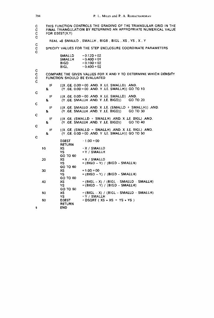
794 P .L . MILLS and P. A. RAMACHANDRAN

C C C C

C C C

C C C C

C

C

C

C

C

THIS FUNCTION CONTROLS THE GRADING OF THE TRIANGULAR GRID IN THE FINAL TRIANGULATION BY RETURNING AN APPROPRIATE NUMERICAL VALUE FOR D3EST(X,Y)

REAL *8 SMALLD , SMALLH , BIGB , BIGL , XS , YS , X , Y

SPECIFY VALUES FOR THE STEP ENCLOSURE COORDINATE PARAMETERS

SMALLD = 0 . 1 2 D + 0 2 SMALLH = 0.40D + 01 BIGD = 0.10D + 02 BIGL = 0.40D + 02

COMPARE THE GIVEN VALUES FOR X AND Y TO DETERMINE WHICH DENSITY FUNCTION SHOULD BE EVALUATED

IF ( (X.GE. 0.0D + 0 0 .AND. X.LE. SMALLD) .AND. & (Y .GE. 0.0D +00 .AND. Y .LE. SMALLH) ) GO TO 10

IF ( (X.GE. 0 . 0 D + 0 0 . A N D . X.LE. SMALLD) .AND. & (Y .GE. SMALLH .AND. Y .LE, BIGD)) GO TO 20

IF &

((X .GE. SMALLD .AND. X .LE. (SMALLD + SMALLH) ) .AND. (Y .GE. SMALLH .AND. Y .LE. BIGD)) GO TO 30

IF &

( (X.GE. (SMALLD + SMALLH) .AND. X.LE. BIGL) .AND. (Y .GE. SMALLH .AND. Y .LE. BIGD)) GO TO 40

IF ((X .GE. (SMALLD + SMALLH) .AND. X .LE. BIGL) .AND. & (Y .GE. 0.0D +00 .AND. Y .LE. SMALLH) ) GO TO 50

10

20

30

40

50

60

D3EST RETURN XS YS GO TO 60 XS YS GO TO 60 XS YS GO TO 60 XS YS GO TO 60 XS YS D3EST RETURN END

= 1.0D + 00

= X / SMALLD = Y / SMALLH

= X / SMALLD = (BIGD - Y) / (BIGD - SMALLH)

= 1.0D + 00 = (BIGD - Y) / (BIGD - SMALLH)

= (BIGL - X) / (BIGL - SMALLD - SMALLH) = ( B I G D - Y ) / ( B I G D - SMALLH)

= (BIGL - X) / (BIGL - SMALLD - SMALLH) =Y / SMALLH =DSQRT ( X S * XS + Y S * Y S )

MATHEMATICAL MODELLING OF CHEMICAL ...Mathematical modelling of chemical engineering systems 771 three-dimensional problems, but approximations to these can be obtained by solving

Documents