Introduction Differential equations Euler method Error analysis Mathematical Modelling Lecture 11 – Differential Equations Phil Hasnip [email protected] Phil Hasnip Mathematical Modelling

Mathematical Modelling Lecture 11 Differential …pjh503/mathematical_model/math...Title Mathematical Modelling Lecture 11 Differential Equations Author Phil [email protected]
Mar 12, 2020
Welcome message from author
This document is posted to help you gain knowledge. Please leave a comment to let me know what you think about it! Share it to your friends and learn new things together.
Transcript
IntroductionDifferential equations
Euler methodError analysis
Mathematical ModellingLecture 11 – Differential Equations
Phil [email protected]
Phil Hasnip Mathematical Modelling

IntroductionDifferential equations
Euler methodError analysis
Overview of Course
Model construction −→ dimensional analysisExperimental input −→ fittingFinding a ‘best’ answer −→ optimisationTools for constructing and manipulating models −→networks, differential equations, integrationTools for constructing and simulating models −→randomnessReal world difficulties −→ chaos and fractals
A First Course in Mathematical Modeling by Giordano, Weir &Fox, pub. Brooks/Cole. Today we’re in chapter 10.
Phil Hasnip Mathematical Modelling
IntroductionDifferential equations
Euler methodError analysis
Change?!
We often have to model dynamic systems.
Discrete −→ difference equationsContinuous −→ differential equations
Today we’re looking at differential equations.
Phil Hasnip Mathematical Modelling

IntroductionDifferential equations
Euler methodError analysis
Change?!
We often have to model dynamic systems.
Discrete −→ difference equationsContinuous −→ differential equations
Today we’re looking at differential equations.
Phil Hasnip Mathematical Modelling
IntroductionDifferential equations
Euler methodError analysis
Differential equations
The basic problem:
dxdt
= x = f (x , t)
subject to given boundary conditions.
Of course we may be interested in higher-order differentialequations!
Phil Hasnip Mathematical Modelling
IntroductionDifferential equations
Euler methodError analysis
Initial value problems
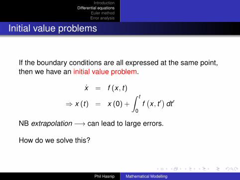
If the boundary conditions are all expressed at the same point,then we have an initial value problem.
x = f (x , t)
⇒ x (t) = x (0) +
∫ t
0f(x , t ′
)dt ′
NB extrapolation −→ can lead to large errors.
How do we solve this?
Phil Hasnip Mathematical Modelling
IntroductionDifferential equations
Euler methodError analysis
General method
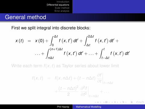
First we split integral into discrete blocks:
x (t) = x (0) +
∫ ∆t
0f(x , t ′
)dt ′ +
∫ 2∆t
∆tf(x , t ′
)dt ′ +
. . .+
∫ (n+1)∆t
n∆tf(x , t ′
)dt ′ + . . .+
∫ t
t−∆tf(x , t ′
)dt ′
Write each term f (x , t) as Taylor series about lower limit
f (x , t) = f (x ,n∆t) + (t − n∆t)∂f∂t
∣∣∣∣t=n∆t
+(t − n∆t)2
2∂2f∂t2
∣∣∣∣t=n∆t
+ . . .
Phil Hasnip Mathematical Modelling
IntroductionDifferential equations
Euler methodError analysis
General method
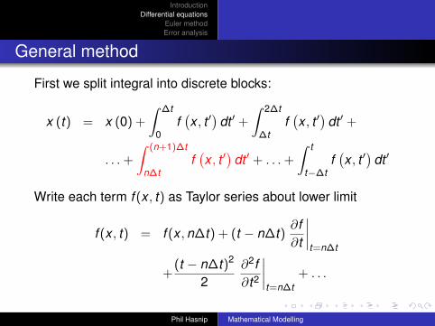
First we split integral into discrete blocks:
x (t) = x (0) +
∫ ∆t
0f(x , t ′
)dt ′ +
∫ 2∆t
∆tf(x , t ′
)dt ′ +
. . .+
∫ (n+1)∆t
n∆tf(x , t ′
)dt ′ + . . .+
∫ t
t−∆tf(x , t ′
)dt ′
Write each term f (x , t) as Taylor series about lower limit
f (x , t) = f (x ,n∆t) + (t − n∆t)∂f∂t
∣∣∣∣t=n∆t
+(t − n∆t)2
2∂2f∂t2
∣∣∣∣t=n∆t
+ . . .
Phil Hasnip Mathematical Modelling
IntroductionDifferential equations
Euler methodError analysis
Euler method
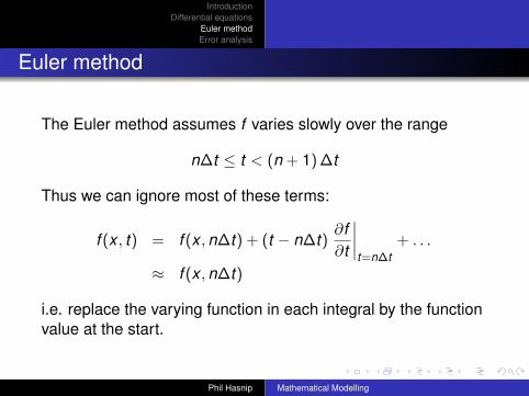
The Euler method assumes f varies slowly over the range
n∆t ≤ t < (n + 1) ∆t
Thus we can ignore most of these terms:
f (x , t) = f (x ,n∆t) + (t − n∆t)∂f∂t
∣∣∣∣t=n∆t
+ . . .
≈ f (x ,n∆t)
i.e. replace the varying function in each integral by the functionvalue at the start.
Phil Hasnip Mathematical Modelling

IntroductionDifferential equations
Euler methodError analysis
Euler method
We can now write:∫ (n+1)∆t
n∆tf(x , t ′
)dt ′ ≈
∫ (n+1)∆t
n∆tf (x (n∆t) ,n∆t) dt ′
= f (x (n∆t) ,n∆t) ∆t
Phil Hasnip Mathematical Modelling

IntroductionDifferential equations
Euler methodError analysis
Example 1: radioactive decay
dxdt
= −λx
which we can solve analytically. However, let’s use Euler –f (x , t) = −λx so we have:
xn+1 = xn + (−λxn)∆t
Let’s see what happens for λ = 1 and ∆t = 0.1.
Phil Hasnip Mathematical Modelling

IntroductionDifferential equations
Euler methodError analysis
Example 1: radioactive decay
λ = 1, ∆t = 0.1:
n tn xn analytic0 0.0 1.0 1.01 0.1 0.90 0.9048372 0.2 0.81 0.818731...
......
...10 1.0 0.348678 0.367879...
......
...50 5.0 0.005154 0.006738
Phil Hasnip Mathematical Modelling
IntroductionDifferential equations
Euler methodError analysis
Example 1: radioactive decay
The error doesn’t seem too bad.
Can reduce error by reducing ∆t −→ more stepsThis error is called truncation errorCan we keep reducing error this way? No!Also have finite precision, or roundoff errorthis limits the final accuracy of any numerical scheme
Phil Hasnip Mathematical Modelling
IntroductionDifferential equations
Euler methodError analysis
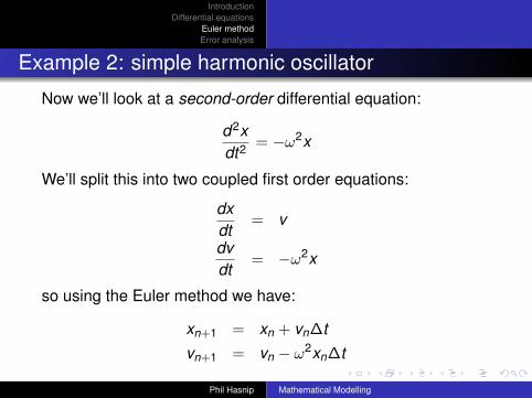
Example 2: simple harmonic oscillator
Now we’ll look at a second-order differential equation:
d2xdt2 = −ω2x
We’ll split this into two coupled first order equations:
dxdt
= v
dvdt
= −ω2x
so using the Euler method we have:
xn+1 = xn + vn∆tvn+1 = vn − ω2xn∆t
Phil Hasnip Mathematical Modelling
IntroductionDifferential equations
Euler methodError analysis
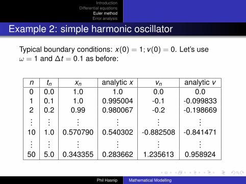
Example 2: simple harmonic oscillator
Typical boundary conditions: x(0) = 1; v(0) = 0. Let’s useω = 1 and ∆t = 0.1 as before:
n tn xn analytic x vn analytic v0 0.0 1.0 1.0 0.0 0.01 0.1 1.0 0.995004 -0.1 -0.0998332 0.2 0.99 0.980067 -0.2 -0.198669...
......
......
...10 1.0 0.570790 0.540302 -0.882508 -0.841471...
......
......
...50 5.0 0.343355 0.283662 1.235613 0.958924
Phil Hasnip Mathematical Modelling
IntroductionDifferential equations
Euler methodError analysis
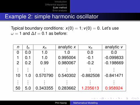
Example 2: simple harmonic oscillator
Typical boundary conditions: x(0) = 1; v(0) = 0. Let’s useω = 1 and ∆t = 0.1 as before:
n tn xn analytic x vn analytic v0 0.0 1.0 1.0 0.0 0.01 0.1 1.0 0.995004 -0.1 -0.0998332 0.2 0.99 0.980067 -0.2 -0.198669...
......
......
...10 1.0 0.570790 0.540302 -0.882508 -0.841471...
......
......
...50 5.0 0.343355 0.283662 1.235613 0.958924
Phil Hasnip Mathematical Modelling

IntroductionDifferential equations
Euler methodError analysis
Example 2: simple harmonic oscillator
Our Euler method leads to a nonphysical velocity v !Clearly something has gone wrong.Why?
Phil Hasnip Mathematical Modelling
IntroductionDifferential equations
Euler methodError analysis
Error analysis for Euler method
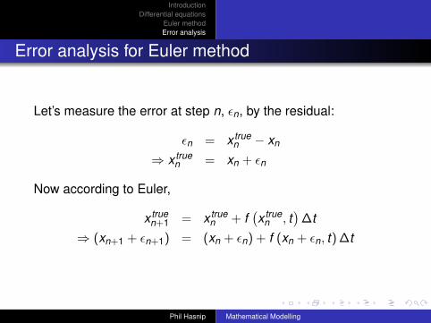
Let’s measure the error at step n, εn, by the residual:
εn = x truen − xn
⇒ x truen = xn + εn
Now according to Euler,
x truen+1 = x true
n + f(x true
n , t)
∆t⇒ (xn+1 + εn+1) = (xn + εn) + f (xn + εn, t) ∆t
Phil Hasnip Mathematical Modelling

IntroductionDifferential equations
Euler methodError analysis
Error analysis for Euler method
Assuming εn is small, we can use a Taylor expansion in x toshow that:
εn+1 = εn
(1 +
∂f∂x
∣∣∣∣x=xn
∆t
)= εnG
where G is the error gain term.
Phil Hasnip Mathematical Modelling
IntroductionDifferential equations
Euler methodError analysis
Error analysis for Euler method
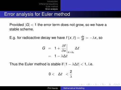
Provided |G| < 1 the error term does not grow, so we have astable scheme.
E.g. for radioactive decay we have f (x , t) = dxdt = −λx , so
G = 1 +∂f∂x
∣∣∣∣x=xn
∆t
= 1− λ∆t
Thus the Euler method is stable if |1− λ∆t | < 1, i.e.
0 < ∆t <2λ
Phil Hasnip Mathematical Modelling

IntroductionDifferential equations
Euler methodError analysis
Beyond Euler
Of course we can do better than Euler:
Predictor-correctorHigher-order methods (extending truncation scheme)
Phil Hasnip Mathematical Modelling
IntroductionDifferential equations
Euler methodError analysis
Beyond Euler
These schemes generally:
Are more accurate and stableAllow larger ∆tRequire more function evaluations per step and morecomputer storage
One common scheme is 4th-order Runge-Kutta – see any texton numerical methods for lots of details!
Phil Hasnip Mathematical Modelling

IntroductionDifferential equations
Euler methodError analysis
Summary
The Euler method can solve differential equationsnumericallyCare must be taken when choosing the time-stepHigher-order methods may be required
Phil Hasnip Mathematical Modelling
Related Documents