MATHEMATICAL MODELLING FOR BIOLOGICAL ...

MATHEMATICAL MODELLING FOR BIOLOGICAL WASTEWATER TREATMENT PLANTS, GAUTENG,

SOUTH AFRICA

Report to the WATER RESEARCH COMMISSION

by

JC NGILA1, AN MATHERI2, V MUCKOYA1, E NGIGI1, F NTULI2, T SEODIGENG2,3 & C ZVINOWANDA1

1Departmen Chemical Science, University of Johannesburg 2Department Chemical Engineering, University of Johannesburg

3Department Chemical Engineering, Vaal University of Technology

WRC Report No 2563/1/19 ISBN 978-0-6392-0114-6

February 2020

ii

Obtainable from Water Research Commission Private Box X03 Gezina, 0031 [email protected] or download from www.wrc.org.za

DISCLAIMER This report has been reviewed by the Water Research Commission (WRC) and approved

for publication. Approval does not signify that the content necessarily reflects the view and policies of the WRC, nor does mention of trade names or commercial products constitute

endorsement or recommendation for use.

© Water Research Commission

mailto:[email protected]

http://www.wrc.org.za/

iii

EXECUTIVE SUMMARY

Emerging contaminants in the water bodies pose a health hazard to the environment and human health. Discharge of effluents from wastewater treatment plants (WWTPs) into water bodies contribute to water pollution. The WWTPs face challenges in removing contaminants in real-time due to the continuously changing process parameters, diversity and pollutant concentrations.

Conventional mathematical modelling and simulation, artificial intelligence/deep learning/machine learning/evolution computation/internet of things (IoT), blockchain, sensor and big data are becoming integral components and essential to describe, predict, forecast and control the complicated interaction of the wastewater treatment processes that are of revolutionized emerging technology breakthrough in the awareness and implementation of the fourth industrial revolution (4IR) era. This is due to complex biological reaction mechanisms, lack of reliable on-line instrumentation, unforeseen changes in microbes, organic and inorganic compounds, multivariable aspects of the real wastewater treatment plant (WWTP) and highly time-varying that create a need for the intelligent technique for analysis of multi-dimensional process data known as the ‘big data’ and diagnoses of inter-relationship of the process variables in the WWTPs. The physical, measured and performance parameters were analysed according to international standards.

Review on the existing models were taken into consideration to reach a consensus concerning the simplest models that possess the capability of realistic predictions of the performance of the activated sludge and biofilm wastewater treatment plant on the nitrification-denitrification, oxygen demand, pH, alkalinity, temperature, mixed liquor of the suspended solids, nitrogen, phosphorus, primary settling, sludge retention time, emerging micropollutants-parabens, chlorination, COD and trace metals in the course of diurnal variations. The database was analyzed to determine bio-kinetic models’ parameters range by considering the specific parameters correlation.

Our study applied mass balance equations, activated sludge model (ASM1) and artificial neural network (ANN) using MATLAB (neural network toolbox), octave, python in prediction of the flow rates, organics (substrate and biomass growth), inorganics, micropollutants and trace metals speciation. This combined knowledge of the process dynamics with the prowess of mathematical methods for evaluation of the operation points, plant dimensions, biochemical parameters interaction with microbes, estimation and identification of the controller parameters had an excellent impact in addressing the challenges posed by the time-varying parameters.

Emphasis was put on the numerical solution’s ability to approximate the analytical solution of the conservation law of mass balance. Calibration of the models was adjusted with the set of influent data in the process of modification of the input data until the simulation models results matched the dataset. Validation was identified to meet the modelling objectives with the level of confidence. The goodness of the prediction (prediction performance) was attained using the coefficient of determination (R2) of 0.98-0.99, sum of square error (SSE) 0.00029-0.1598, room mean-square error (RMSE) of 0.0049-0.8673 and mean squared error (MSE) 2.7059e-14 to

iv

2.3175e-15. The models were found to be a robust tool for predicting WWTP performance. This revealed that the influent indices could be applied to the prediction of the effluent quality (EQ). The overall models were used to detect the inconsistency within the WWTP datasets through identification and confirmation of the mass flow into and out of the systems. The modelling and computation of the speciation of compounds offered an extremely powerful tool for the process design, data handling, troubleshooting and optimization representing a multivariable system that cannot be effectively handled without appropriate modelling, computer-based techniques and procurement for the best compliance with international standards plant upgrades efficiency and diversification.

The approach can also be used to handle many other types of waste treatment systems, environmental management, carbon capture and emerging technologies so as to meet the cost-effectiveness, environmental, technical criteria and wide range of big data support in the implementation of the national and sustainable development goals (SDGs).

The above summary highlights work done by the main doctoral student, whose project is entitled Mathematical modelling of biological wastewater treatment process and bioenergy production.

In Appendices F and G, we present a summary of studies by two other students under the WRC project. These studies covered (i) Method development of analytical techniques for sample analysis and (ii) Degradation of organics in the WWTP, using nanotechnology.

Briefly, for analysis of contaminants in the wastewater samples, we investigated multivariate-based optimization techniques for sample preconcentration using solid phase extraction (SPE) and dispersive liquid-liquid microextraction (DLLME) followed by chromatography-mass spectrometry techniques for quantification of parabens and polyaromatic hydrocarbons in the wastewater treatment plant. We also investigated the performance of tungsten trioxide (WO3) nanomaterials modified with various nanoparticles, to produce iron-doped WO3, cadmium sulphide-doped-WO3, and Z-scheme cobalt oxide-tungsten oxide (Co3O4/WO3) nanocomposites for the photocatalytic degradation of parabens and methylene blue. The best photodegradation results were produced with Z-scheme Co3O4/WO3 nanocomposite.

v

ACKNOWLEDGEMENTS Reference Group Members: Dr John Zvimba Water Research Commission (Chairperson) Prof Morris Onyango Department of Chemical Engineering, Tshwane University of Technology Dr Caliphs Zvinowanda Department of Chemical Science, University of Johannesburg Prof Richard Moutloali Department of Chemical Science, University of Johannesburg Prof Craig Sheridan University of the Witwatersrand Prof Thokozani Majozi University of the Witwatersrand Mr Kerneels C.M. Esterhuyse City of Tshwane: Water & Sanitation/Wastewater Treatment Works, Daspoort Prof Bobby Naidoo Department of Chemistry: Vaal University of Technology Prof Ochieng Aoyi Department of Chemical Engineering: Vaal University of Technology/Botswana International University of Science and Technology (BIUST) Mr Bennie Mokgonyana Water Research Commission Mr Nico van Blerk East Rand Water Care Association (ERWAT) Mr James Topkin East Rand Water Care Association (ERWAT) Mr Masilo Shai and Mr Mthokozisi Success Mahlalela (Operators) – City of Tshwane: Water & Sanitation/Wastewater Treatment Works, Daspoort Ms Sharene Janse van Rensburg – WaterLab

The following were supported by the WRC under the current project:

• Dr Anthony Njuguna Matheri PhD student’s project – Department of Chemical Engineering, University of Johannesburg

• Dr Geoffrey Bosire Post Doc – Department of Chemical Science, University of Johannesburg

• Dr Eric Ngigi PhD student’s project – Department of Chemical Science, University of Johannesburg

• Dr Valerie Muckoya PhD student’s project – Department of Chemical Science, University of Johannesburg

• Mr Solomon Pole MTech student’s project – Department of Chemical Science, University of Johannesburg

vi

This page was intentionally left lank

vii

TABLE OF CONTENTS

EXECUTIVE SUMMARY ..................................................................................................... iii ACKNOWLEDGEMENTS ....................................................................................................... v

LIST OF FIGURES ............................................................................................................... xiii

LIST OF TABLES ................................................................................................................... xv

LIST OF ABBREVIATIONS ................................................................................................. xvi LIST OF COMPUTATIONAL TOOLS ................................................................................. xxi

CHAPTER 1: INTRODUCTION ............................................................................................ 1

1.1 Background ................................................................................................................. 1

1.2 Aims and Objectives ................................................................................................... 5

1.2.1 Aims of the study ................................................................................................. 5 1.2.2 Objectives of the study......................................................................................... 6

CHAPTER 2: LITERATURE REVIEW ................................................................................. 7

2.1 Introduction ................................................................................................................. 7

2.2 Wastewater Treatment Plants in Gauteng Province, South Africa ............................. 7 2.2.1 Description of Distribution of WWTPs ............................................................... 8

2.2.2 The distribution of wastewater treatment works in Gauteng province ................ 9

2.3 Wastewater Treatment Processes .............................................................................. 16

2.3.1 Components of wastewater treatment plants ..................................................... 16 2.3.2 Classification of treatment methods................................................................... 16

2.3.3 Physical, chemical and biological characteristics of wastewater and their source. ................................................................................................................ 19

2.4 Mechanisms of the Treatment Processes .................................................................. 20

2.4.1 Sedimentation .................................................................................................... 21

2.4.2 Coagulation ........................................................................................................ 21 2.4.3 Filtration ............................................................................................................. 21

2.4.4 Disinfection ........................................................................................................ 21

2.4.5 Softening ............................................................................................................ 21

2.4.6 Aeration.............................................................................................................. 22 2.4.7 Trace elements removal ..................................................................................... 22

2.4.8 Anaerobic digestion ........................................................................................... 22

2.5 Technique used in Selecting Plants to Sample .......................................................... 25

viii

2.5.1 Multi-criteria decision analysis (MCDA) .......................................................... 25

2.6 Designs to be Considered in Selecting a WWTP ...................................................... 26

2.6.1 Establishment of design criteria ......................................................................... 27 2.6.2 Environmental and regulatory ............................................................................ 27

2.6.3 Wastewater characteristics ................................................................................. 27

2.6.4 System reliability ............................................................................................... 28

2.6.5 Site limitation ..................................................................................................... 28 2.6.6 Design life .......................................................................................................... 28

2.6.7 Cost .................................................................................................................... 28

2.7 Classification of WWTPs according to nature of influent ........................................ 28

2.7.1 Domestic or sanitary wastewater ....................................................................... 28 2.7.2 Industrial wastewater ......................................................................................... 28

2.7.3 Infiltration and inflow ........................................................................................ 29

2.7.4 Storm water ........................................................................................................ 29

2.8 Tracer Techniques and their Utilization in Wastewater Treatment Plants ................ 29 2.8.1 The success of radiotracer application depend on (IAEA, 2011a): ................... 30

2.8.2 Residence time distribution calculation using a tracer ...................................... 31

2.9 Economic Benefits of the Tracer Utilization in Wastewater Treatment Plant .......... 33

2.10 Conventional Tracer for WWTPs ............................................................................. 34 2.10.1 Chemical tracer .................................................................................................. 34

2.10.2 Optical tracers .................................................................................................... 34

2.11 Radioactive versus Conventional Tracer Techniques, Applied to WWTPs (IAEA, 2011a). ....................................................................................................................... 35

2.12 Modelling and Simulation of Wastewater Treatment Process .................................. 37

2.12.1 Models................................................................................................................ 37 2.12.2 Advantage of modelling in wastewater treatment processes ............................. 39

2.12.3 Mass balance analysis ........................................................................................ 39

2.12.4 Different types of models................................................................................... 42

2.12.5 Bio-chemical kinetics models ............................................................................ 42 2.12.6 Identification of constraints for the modelling scenarios:.................................. 43

2.13 Standards of Organics and Inorganics in Wastewater ............................................... 43

2.14 Sources of Trace Metals in Wastewater Treatment Plant ......................................... 45

2.15 Levels of Metals in WWTPs in Gauteng .................................................................. 45 2.16 Organic Compounds in Water and Sludge in WWTPs, Gauteng Province .............. 50

2.16.1 Polyaromatic hydrocarbons (PAHs) .................................................................. 50

ix

2.16.2 Pesticides............................................................................................................ 51

2.16.3 Disinfection by-products .................................................................................... 52

2.16.4 Personal care products ....................................................................................... 53 2.16.5 Parabens ............................................................................................................. 54

2.17 Production of Organic Compounds in Wastewater Sludge (WWS) ......................... 56

2.17.1 Occurrence of organic contaminants in wastewater sludge ............................... 57

2.17.2 Removal/biodegradation of organic contaminants in wastewater sludge (WWS) ............................................................................................................................ 58

2.18 Environmental and health impacts of organic contaminants in wastewater and wastewater sludge ..................................................................................................... 59

CHAPTER 3: MATHEMATICAL MODELLING AND MASS BALANCE FOR THE ORGANIC AND INORGANIC COMPOUNDS IN THE WASTEWATER TREATMENT PROCESSES ........................................................................................................................ 60

3.1 Summary ................................................................................................................... 60

3.2 Modelling Framework for Wastewater Treatment Processes ................................... 61

3.3 Wastewater Treatment Plant’s Selection and Sampling Positions ............................ 62

3.3.1 Questionnaire development and site identification ............................................ 62 3.3.2 Site reconnaissance (surveying) ......................................................................... 63

3.3.3 Site dimension .................................................................................................... 63

3.3.4 Identification of the sampling positions ............................................................. 64

3.4 Experimental Procedures........................................................................................... 64 3.4.1 Material, chemical and apparatus ...................................................................... 65

3.4.2 Equipment used for the wastewater analysis ..................................................... 66

3.4.3 Computation tools used in simulation modelling .............................................. 66

3.5 Wastewater Sample Preparation and Analysis .......................................................... 67 3.5.1 Sample source .................................................................................................... 67

3.5.2 Sampling procedure ........................................................................................... 67

3.5.3 Sample storage ................................................................................................... 67

3.5.4 Sample analysis .................................................................................................. 67 3.6 Wastewater Treatment Process Model Set-up .......................................................... 71

CHAPTER 4: MATHEMATICAL MODELLING AND MASS BALANCE FOR THE ORGANIC AND INORGANIC COMPOUNDS IN THE WASTEWATER TREATMENT PROCESSES ........................................................................................................................ 72

4.1 Summary ................................................................................................................... 72

4.2 Introduction ............................................................................................................... 73

4.3 Modelling .................................................................................................................. 74

x

4.3.1 A State-of-the-art model .................................................................................... 74

4.3.2 Conventional mathematical modelling .............................................................. 76

4.4 Experimental Procedures........................................................................................... 77 4.4.1 Mass balance of wastewater treatment plant ..................................................... 77

4.4.2 Primary settlement sizing and velocity .............................................................. 78

4.4.3 Organic volumetric loading rate ........................................................................ 78

4.4.4 Sludge retention time or sludge age ................................................................... 78 4.4.5 Specific organic loading rate ............................................................................. 79

4.4.6 Effect of temperature on metabolic activity ....................................................... 79

4.4.7 Effect of pH on metabolism ............................................................................... 79

4.4.8 Biomass concentration mass balance ................................................................. 80 4.4.9 Substrate mass balance ...................................................................................... 80

4.4.10 Mixed liquor solids concentration and solids production (MLVSS) mass balance ............................................................................................................................ 80

4.4.11 Nitrogen biological removal mass balance ........................................................ 81

4.4.12 Biological phosphorus removal ......................................................................... 82

4.4.13 Oxygen demand mass balance ........................................................................... 83 4.4.14 Biological removal of recalcitrant and trace organic compounds ..................... 83

4.4.15 Disinfectants used in the wastewater treatment ................................................. 84

4.4.16 Food to microorganism ratio .............................................................................. 84

4.4.17 Removal efficiency of the organic compounds’ removal .................................. 85 4.4.18 Calibration and validation .................................................................................. 85

4.5 Results and Discussions ............................................................................................ 85

4.5.1 Modelling analysis using microbial growth kinetics, mass balance, and activated sludge model No. 1 of the WWTP ...................................................... 85

4.5.2 Impact of primary settlement sizing and velocity .............................................. 86 4.5.3 Change of design flowrate (loading) with the hydraulic retention time ............ 86

4.5.4 Effect of the solid retention time in the WWTP ................................................ 88

4.5.5 Effect of temperature on microbial growth ........................................................ 89

4.5.6 Impact of pH and pH dependency at the WWTP .............................................. 90

4.5.7 Seasonal variation of the total alkalinity ............................................................ 93 4.5.8 Impact of the electrical conductivity.................................................................. 94

4.5.9 Fate and transport of emerging organics compounds ........................................ 96

4.5.10 Degradation of the organic matter inform of chemical oxygen demand ........... 97

4.5.11 Effect of the mixed liquor suspended solids .................................................... 102

xi

4.5.12 Impact of total suspended solids in the concentration of suspended solid fraction ............................................................................................................. 103

4.5.13 Variation of the volatile suspended solids in WWTP ....................................... 104

4.5.14 Effect of dissolved oxygen in the wastewater treatment processes ................. 105 4.5.15 Sequence in the biological nitrogen removal ................................................... 107

4.5.16 Effect of biological phosphorus removal ......................................................... 113

4.5.17 Behavior of sulphates in wastewater treatment plant ...................................... 116

4.5.18 Impact of chlorides in the disinfection of the wastewater ............................... 116 4.5.19 Impact of food and microbial (f/m) ratio and the efficiency of nutrients removal .......................................................................................................................... 118

4.6 Conclusion ............................................................................................................... 120

CHAPTER 5: TRACE METALS SPECIATION MODELLING IN THE WASTEWATER TREATMENT PROCESSES: GEOCHEMICAL MODELLING ........................................ 122

5.1 Summary ................................................................................................................. 122

5.2 Introduction ............................................................................................................. 122 5.3 Geochemical Modelling .......................................................................................... 124

5.4 Material and Methods.............................................................................................. 125

5.4.1 Analytical methods for trace metals ................................................................ 126

5.5 Results and Discussion ............................................................................................ 127 5.5.1 Trace metals mass balance ............................................................................... 127

5.5.2 Speciation of the trace metals .......................................................................... 129

5.6 Conclusion ............................................................................................................... 134

CHAPTER 6: AI-BASED BASED PREDICTION MODEL FOR TRACE METALS AND COD IN THE WASTEWATER TREATMENT USING ARTIFICIAL NEURAL NETWORKS ...................................................................................................................... 135

6.1 Summary ................................................................................................................. 135 6.2 Introduction ............................................................................................................. 135

6.3 Hybrid AI Techniques ............................................................................................. 137

6.4 Methodology ........................................................................................................... 138

6.4.1 Concept of deep learning (machine learning) with AI-modelling using artificial neural network ................................................................................................. 138

6.4.2 Model performance evaluation ........................................................................ 140 6.5 Results and Discussion ............................................................................................ 141

6.5.1 Effect of trace metals and chemical oxygen demand in the wastewater treatment process.............................................................................................................. 141

6.5.2 Process performance prediction ....................................................................... 145

6.6 Conclusion ............................................................................................................... 150

xii

CHAPTER 7: CONCLUSIONS AND RECOMMENDATIONS ...................................... 151

7.1 Conclusions ............................................................................................................. 151

7.2 Recommendations ................................................................................................... 153 REFERENCES ...................................................................................................................... 163

APPENDICES ....................................................................................................................... 180

Appendix A: Questionnaire on Selection of the Wastewater Treatment Plants ................ 180

Appendix B1: The Activated Sludge Model (ASM) No. 1 under International Association of Water Quality (IAWQ) ....................................................................................................... 189 Appendix B2: Activated Sludge Model No.1 Spreadsheet ................................................ 190

Appendix B3: Wastewater Treatment Plant Simulator ...................................................... 191

Appendix C: Daspoort Wastewater Treatment Plant: Site Survey, Tracer Application and Sampling Program .............................................................................................................. 192

Appendix D: Local and International Effluent Discharge Standards and the Specification ............................................................................................................................................ 193

Appendix E: Local and International Effluent Discharge Standards and the Specification ............................................................................................................................................ 195

Appendix F: Analytical Techniques for Montoring Water Pollutants……………………197

Appendix G: Photocatalytic Degration of Water Contaminants Using Nanomaterials…..204

xiii

LIST OF FIGURES

Figure 1.1: Distribution of WWTPs in Gauteng Province, South Africa (Department of Water Affairs, Accessed 2016). ............................................................................................................ 2 Figure 1.2: Gauteng province among other South African Provinces with a Provincial green drop score of 78.8% ................................................................................................................... 4 Figure 2.1: The map gives the geographic location of the Gauteng Province in relation to the other provinces in the country.................................................................................................... 7 Figure 2.2: Size distribution of wastewater treatment plants in South Africa ........................... 8 Figure 2.3: The status and distribution of wastewater treatment works in Gauteng linked to density, economies of scale and centralization engineering philosophy ................................... 9 Figure 2.4: General wastewater treatment process units operation (E. Metcalf). .................... 17 Figure 2.5: General schematic diagram of an activated sludge process .................................. 18 Figure 2.6: Flow diagram for unit operation and processes in physical, chemical and biological processes used in wastewater treatment (E. Metcalf). ............................................ 19 Figure 2.7: Degradation steps of anaerobic digestion process (Angelidaki et al., 1996). ....... 23 Figure 2.8: Principles of tracer residence time distribution (RTD) (de Souza Jr & Lorenz; I.A.E.A., 2011a)……………………………………………………………………………...31 Figure 2.9: Residence time distribution curve behaviour……………………………………32 Figure 2.10: Generic steps followed in henerating the model (Eva, 2010; Sanders, Veeken, Zeeman & van Lier, 2003)…………………………………………………………………...38 Figure 2.11: Mass balanceon its associate inouts and outputs……………………………….41 Figure 3.1: Modelling framework for wastewater treatment process ...................................... 61 Figure 3.2: Framework for the wastewater treatment process plant selection and the sampling positions ................................................................................................................................... 62 Figure 3.3: Multi-criteria decision analysis (MCDA) on the wastewater treatment process... 63 Figure 3.4: Framework for the development of the samplings programme, sample analysis and mass balance model........................................................................................................... 65 Figure 3.5: Overview of the modelling process ....................................................................... 71 Figure 4.1: Change of flow rates with HRT in the activated sludge wastewater treatment plant.................................................................................................................................................. 86 Figure 4.2: Change of flow rates and HRT in the biofilm wastewater treatment plant ........... 87 Figure 4.3: Seasonal sludge retention time for the wastewater treatment plant ...................... 88 Figure 4.4: Variation of seasonal temperature and reaction rate coefficient at the reaction temperature .............................................................................................................................. 89 Figure 4.5: Change of pH in the activated sludge WWTP ...................................................... 91 Figure 4.6: Change of pH in the biofilm WWTP..................................................................... 91 Figure 4.7: The seasonal variation of the pH and pH dependency in the wastewater treatment process...................................................................................................................................... 92 Figure 4.8: Total alkalinity of the wastewater treatment plant ................................................ 93 Figure 4.9: Electrical conductivity of the activated sludge WWTP ........................................ 94 Figure 4.10: Electrical conductivity of the biofilm WWTP .................................................... 95 Figure 4.11: Seasonal variation of electrical conductivity in the WWTP ............................... 95 Figure 4.12: Emerging micropollutants in the activated sludge WWTP ................................. 96 Figure 4.13: Emerging micro-pollutants in the biofilm WWTP .............................................. 97 Figure 4.14: Modelling of organic compounds in the activated sludge of the WWTP ........... 98

xiv

Figure 4.15: Modelling of organic compounds in the biofilm of the WWTP ......................... 99 Figure 4.16: Biological nutrient removal informs of COD from activated sludge WWTP .. 101 Figure 4.17: Biological nutrient removal informs of COD from biofilm WWTP ................. 101 Figure 4.18: Seasonal variation of the total suspended solids in the wastewater treatment plant................................................................................................................................................ 103 Figure 4.19: Seasonal variation of the volatile suspended solids-mixed mixed liquor of the WWTP. .................................................................................................................................. 104 Figure 4.20: Dissolved oxygen demand of the activated sludge WWTP .............................. 105 Figure 4.21: Dissolved oxygen demand of the biofilm WWTP ............................................ 106 Figure 4.22: Seasonal variation of the nitrates and nitrites as N in the WWTP .................... 108 Figure 4.23: Seasonal variation of the total Kjeldahl nitrogen in the WWTP ....................... 110 Figure 4.24: Variation of the TKN in the biological nutrient removal .................................. 111 Figure 4.25: Seasonal variation of the free and saline ammonium as N in the WWTP ........ 112 Figure 4.26: Seasonal variation of the free and saline ammonium as N for the mixed liquor in the WWTP ............................................................................................................................. 113 Figure 4.27: Effect of phosphate in the biological in-between process units of the wastewater treatment plant ....................................................................................................................... 114 Figure 4.28: Effect of phosphate inflow and outflow in the wastewater treatment plant ...... 115 Figure 4.29: Presence of sulphates in the wastewater treatment plant .................................. 116 Figure 4.30: Presence of chlorine in the wastewater treatment plant .................................... 117 Figure 4.31: Seasonal nutrient removal efficiency and the ratio of food to the microorganism of the activated sludge WWTP .............................................................................................. 118 Figure 4.32: Seasonal nutrient removal efficiency and the ratio of food to the microorganism of the biofilm WWTP ............................................................................................................ 119 Figure 5.1: Completely mixed reactor in series in the WWTP .............................................. 128 Figure 5.2: Speciation of the trace metals in the activated sludge plant ................................ 129 Figure 5.3: Speciation of the trace metals in the biofilm plant .............................................. 130 Figure 5.4: Daily variation of trace metals contents in the influence of the biofilm wastewater treatment plants ...................................................................................................................... 132 Figure 5.5: Daily variation of trace metals contents in the influence of the activated sludge wastewater treatment plants ................................................................................................... 133 Figure 6.1: Flow diagram of the concept of deep learning (machine learning) with AI-modelling using artificial neural network .............................................................................. 138 Figure 6.2: Schematic of the artificial neural network in AI-modelling using deep learning139 Figure 6.3: Trace metals speciation in the effluent wastewater treatment process ................ 142 Figure 6.4: The concentration of the effluent chemical oxygen demand (COD) in the wastewater treatment process ................................................................................................ 143 Figure 6.5: Function fit of the variation of the trace metals .................................................. 144 Figure 6.6: Function fit of the variation of the COD ............................................................. 144 Figure 6.7: Performance training and overfitting test of the datasets and prediction using regression R for the trace metals (network regression) ......................................................... 146 Figure 6.8: Validation performance of the trace metals using mean squared error ............... 147 Figure 6.9: Performance training and overfitting test of the datasets and prediction using regression R for the chemical oxygen demand ...................................................................... 148 Figure 6.10: Validation performance of the COD using mean squared error ........................ 149

xv

LIST OF TABLES

Table 1.1: Wastewater treatment plants distribution in Gauteng Province (Department of Water Affairs, Accessed 2016). ................................................................................................. 2 Table 2.1: The breakdown of municipal-owned WWTPs in Gauteng in terms of size and location ..................................................................................................................................... 10 Table 2.2: List of WWTPs in Gauteng with names of the plants, responsible authority, Municipality and the operating capacity – whether 100% performance or exceeding the design flow: .............................................................................................................................. 11 Table 2.3: A quick overview of the Standards NOT being met by the various WWTPs in Gauteng, as captured at the Department of Water Affairs and Forestry (DWAF, 2008) Regional Office. NB. ............................................................................................................... 13 Table 2.4: Important contaminants of concern in wastewater treatment (Henze & Comeau, 2008; E. Metcalf) ..................................................................................................................... 20 Table 2.5: Unit operation and processes in wastewater treatment plants (E. Metcalf)………24 Table 2.6: Saaty's scale intensity 1-9 (Saaty, 2004)………………………………………….26 Table 2.7: Comparison of radioactive and conventional tracer techniques using gas tracers in the WWTP (I.A.E.A., 2011a)………………………………………………………………...35 Table 2.8: Comparison of radioactive and conventional tracer techniques using liquid tracers in the WWTP (I.A.E.A., 2011a)……………………………………………………………..36 Table 2.9: Comparison of radioactive and conventional tracer techniques using solid tracers in the WWTP (I.A.E.A., 2011a)……………………………………………………………..37 Table 2.10: The metals of importance in wastewater managements………………………...44 Table 2.11: Discharge Standards Guidelines………………………………………………...47 Table 2.12: Metal contents (mg L-1) raw effluent from selected Gauteng WWTPs (City of Tshwane Data from 2011-2013)……………………………………………………………..48 Table 2.13: Metal contents (µg L-1) in treated effluent from selected Gauteng WWTPs (City of Tshwane Data from 2011-2013)…………………………………………………………..49 Table 2.14: Levels of Metals (mg L-1) in sludge from selected Gauteng WWTPs (City of Tshwane Data from 2011-2013)……………………………………………………………..49 Table 4.1: Kinetic constant and their temperature sensitivity for Autotrophic Nitrifier Organisms (ANO) for the ASM models .................................................................................. 81

xvi

LIST OF ABBREVIATIONS

Abbreviation Description ACN Acetonitrile ASMs Activated Sludge Models ASP Activated Sludge Process ANFIS Adaptive Neuro-Fuzzy Inference Systems APHA America Public Health Association AWWA American Water Works Association AA Amino Acid NH4-N Ammonia Nitrogen AD Anaerobic Digestion ADM Anaerobic Digestion Model AHP Analytic Hierarchy Process ANP Analytical Network Process AI Artificial Intelligence ANN Artificial Neural Network AMPTS 11 Automatic methane Potential Test System Machine ANO Autotrophic Nitrifier Organisms ADWF Average Dry Weather Flow BAT Best Available Technology BMPs Best Management Practices BMP Bio-chemical Methane Potential BOD Biochemical Oxygen Demand BPR Biological Phosphorus Removal BPC Bio-Process Control CV Calorific Value CHP Combine Heat and Power CHNS Carbon Hydrogen Nitrogen Sulphur CODH Carbon Monoxide Dehydrogenase C/N Carbon to Nitrogen Ratio CNHS Carbon, Nitrogen, Hydrogen and Sulphur CNSP Carbon, Nitrogen, Sulphur and Phosphorus CBR Case-Based Reasoning COD Chemical Oxygen Demand CoJ City of Johannesburg CoT City of Tshwane CSOs Combined Sewer Overflows CMAS Completely Mixed Activated Sludge CFD Computer Fluid Dynamics CGI Computer Generated Imagery CI Consistency Index CR Consistency Ration

xvii

CS Cryogenic Separation CW Constructed Wetlands CSTR Continuous Stirred Tank Reactor CRR Cumulative Risk Rating QDW Daily Quantity of Waste DMA Decision Matrix Approach DSS Decision Support Systems DESTA Decision Support Tool for Aquaculture TU Delft Delft University of Technology DNA Deoxyribonucleic Acid DWA Department of Water Affairs DCM Dichloromethane DE Differential Equation DCL Digestion Chamber Loading LDC Digestion Chamber Loading (kg of TS or VS/m3 of digestion chamber volume. day) DRB 200 Digital Digester DR 3900 Digital Programmable Analyzer DMU Discharge of Pumping and Mixing Unit DBPs Disinfection By-Products DO Dissolved Solids DAI Distributed Artificial Intelligent DS Dry Solids E Efficiency EC Electrical Conductivity EP Emerging Pollutant EDSS Environmental Decision Support Systems EPA Environmental Protection Agency ES Expert System EA External Aeration FM/AM Facilities Management/Automated Mapping FSIEG Financial Stability, Innovation and Economic Growth FAAS Flame Atomic Absorption Spectrometry F/M food and microorganism ratio HCHO Formaldehydes FIR Fourth Industrial Revolution FSA Free and Saline Ammonia FIS Fuzzy Inference System FL Fuzzy Logic GC Gas Chromatography GC-MS Gas Chromatography-Mass Spectrometer GA Genetic Algorithms GIS Geographical Information Systems GP Goal Programming GFAAS Graphite Furnace Atomic Absorption Spectrometry

xviii

GHG Greenhouse Gas GUA Growing Up Africa HSE Health, Safety and Environment HP-LC High-Performance Liquid Chromatograph HRT Hydraulic Retention Time Hydroponic hydroculture IPP Independent Power Producer ICP-MS Inductively Coupled Plasma-Mass Spectrometry ICP-OES Inductively Coupled Plasma-Optical Emission Spectroscopy IWC Influent Waste Concentration CIW Influent Waste Concentration (kg of TS or VS/m3 of digestion chamber volume) IH Innovation Hub ITSS Inorganic Total Suspended Solids ICA Instrumentation, Control and Automation IMSW-MS Integrated Municipal Solid Waste Management Systems IWM Integrated Waste Management IAEA International Atomic Energy Agency IBM International Business Machines Corporation IWA International Water Association KBS Knowledge-Based System KSOFM Kohonen Self-Organization Feature Maps LCMS Liquid Chromatography-Mass Spectrometer LCFA Long Chain Fatty Acids MAB Microalgae Biofixation MCLs Maximum Contaminants Level MBR Membrane Bioreactor MeOH Methanol MLSS Mixed Liquor Suspended Solids MLVSS Mixed Liquor Volatile Suspended Solids MC Moisture Content MS Monosaccharaides MCSM Monte Carlos Simulation Model MADM Multi-Attributes Decision Making MAPE Mean Absolute Percentage Error MCDA Multi-Criteria Decision Analysis MAIS Multi-Layered Artificial Immune Systems MODSS Multiple Objective Decision Support Systems MT Membrane Technology MSW Municipal Solid Waste MSE Mean Squared Error NOM Natural Organic Matter NNOs Nitrite to Nitrate nbVSS Nonbiodegradable Volatile Suspended Solids NGO Non-Government Organization

xix

OLI Open Learning Initiatives OASIS Operation Assistant and Simulated Intelligent System OFMSW Organic Fraction of Municipal Solid Waste OLD Organic Loading Rate PSA Pressure Swing Adsorption PPE Personal Protection Equipment PO4

3- Phosphates PFR Plug Flow Reactor PAHs Polycyclic Aromatic Hydrocarbon PS Pond System PEI Potential Environmental Impact PR Probabilistic Reasoning PEETS Process Energy Environmental Technology Station PFD Process Flow Diagram R&D Research and Development RI Random Index RDBMSs Relational Database Management Systems RAMS+CH Reliability, Availability, Maintainability, Safety and Plus Cost, Human Resource RS Remote Sensing REIPPPP Renewable Energy Independent Power Producer Procurement Programme RNG Renewable Natural Gas RTD Residence Time Distributions RNA Ribonucleic Acid RAC Risk Assessment Codes RBC Rotating Biological Contractors RMSE Root Mean Square Error RST Rough Set Theory RBS Rule-Based Reasoning SDWA Safe Drinking Water Act SSOs Sanitary Sewer Overflows SBR Sequencing Batch Reactors SMART Simple Multi-Attribute Rating Technique SRT Sludge Retention Time SCT Soft Computing Techniques SPE Solid Phase Extraction SABIA South Africa Biogas Industry Association SANS South Africa National Standards SMA Specific Methanogenic Activity SSE Sum of Square Error SVM Support Vector Machine SDG Sustainable Development Goal TUT Technical University of Tshwane TOPSIS Technique for Order Preference by Similarities to Ideal Solution TCD Thermal Conductivity Detector

xx

TDS Total Dissolved Solids TAC Total inorganic acids TKN Total Kjeldahl Nitrogen TOC Total Organic Carbon TP Total Phosphorus TN Total Solids TS Total Solids TSC Total Solids Concentration in digester TSW Total Solids Concentration of waste TSS Total Suspended Solids TF Trickling Filter THMs Trihalomethanes UV Ultraviolet Radiation UNEP United Nation Environmental Programme UNICEF United Nations Children Funds UNDP United Nations Development Programme UNIDO United Nations Industrial Development organization UCT University of Cape Town UJ University of Johannesburg UP University of Pretoria Wits University of Witwatersrand UASB Up-flow Anaerobic Sludge Blanket Reactor VUT Vaal University of Technology VBA Visual Basic Applications VFA Volatile Fatty Acid VOC Volatile organic acids VS Volatile Solids VSS Volatile Suspended Solids VDC Volume of Digestion Chamber WAR Waste Reduction Algorithms WWTP Wastewater Treatment Plant WPCF Water Pollution Control Federation WRC Water Research Commission WRRFs Water Resource Recovery Facilities WSM Weighted-Sum Method WBG World Bank Group WHO World Health Organization

xxi

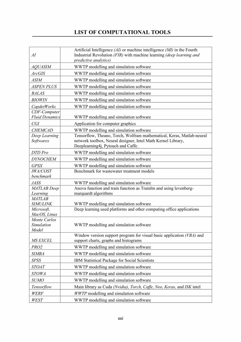
LIST OF COMPUTATIONAL TOOLS

AI

Artificial Intelligence (AI) or machine intelligence (MI) in the Fourth Industrial Revolution (FIR) with machine learning (deep learning and predictive analytics)

AQUASIM WWTP modelling and simulation software ArcGIS WWTP modelling and simulation software ASIM WWTP modelling and simulation software ASPEN PLUS WWTP modelling and simulation software BALAS WWTP modelling and simulation software BIOWIN WWTP modelling and simulation software CapdetWorks WWTP modelling and simulation software CDF-Computer Fluid Dynamics WWTP modelling and simulation software CGI Application for computer graphics CHEMCAD WWTP modelling and simulation software Deep Learning Softwares

Tensorflow, Theano, Torch, Wolfram mathematical, Keras, Matlab-neural network toolbox, Neural designer, Intel Math Kernel Library, Deeplearning4j, Pytouch and Caffe.

DTD Pro WWTP modelling and simulation software DYNOCHEM WWTP modelling and simulation software GPSX WWTP modelling and simulation software IWA/COST benchmark

Benchmark for wastewater treatment models

JASS WWTP modelling and simulation software MATLAB Deep Learning

Anova function and train function as Trainlm and using levenberg-marquardt algorithms

MATLAB SIMULINK WWTP modelling and simulation software Microsoft, MacOS, Linux

Deep learning used platforms and other computing office applications

Monte Carlos Simulation Model

WWTP modelling and simulation software

MS EXCEL Window version support program for visual basic application (VBA) and support charts, graphs and histograms

PRO2 WWTP modelling and simulation software SIMBA WWTP modelling and simulation software SPSS IBM Statistical Package for Social Scientists STOAT WWTP modelling and simulation software STOWA WWTP modelling and simulation software SUMO WWTP modelling and simulation software Tensorflow Main library as Cuda (Nvidia), Torch, Caffe, Neo, Keras, and ISK intel WERF WWTP modelling and simulation software WEST WWTP modelling and simulation software

xxii

This page was intentionally left blank

1

CHAPTER 1: INTRODUCTION

1.1 Background

The population growth, economic development, urbanization, improvement in living-

standards, awareness and in the implementation of the fourth industrial revolution (FIR) has

increased waste generation and introduced emerging contaminants into waste streams that may

pose sanitary and environmental risks (Al-Khatib, Monou, Zahra, Shaheen & Kassinos, 2010;

Amin, 2009; Matheri et al., 2018). These contaminants have increased the demand for

specialized emerging pollutants (EPs) removal techniques in wastewater. The emerging

contaminants of concern include (trace metals, personal care products, endocrine disruption

chemicals, flame retardants, pesticides, pharmaceutical, plasticizers, various fluorinated

compounds, nanomaterial, etc.) that has led to more stringent regulations on wastewater

discharge quality parameters (Stamou & Antizar-Ladislao, 2016). These contaminants end up

in water bodies and landfills, leading to pollution of the environment thus putting a strain on

health, economic and social sectors (Lemoine et al., 2013; Stamou & Antizar-Ladislao, 2016).

The rapid increase in the quantities of waste generated demand a wider coverage of existing

waste management system that provides sustainable standards for innovative technologies for

treatment. Achieving these standards requires the quantitative characterization of given waste

streams, implementation of innovative integrated waste management systems and reliable

waste management data which provides an all-inclusive resource for a comprehensive, critical

and informative evaluation of waste management options in all waste management

programmes (N.-B. Chang & Davila, 2008; Miezah, Obiri-Danso, Kádár, Fei-Baffoe &

Mensah, 2015; Ojeda-Benítez, Armijo-de Vega & Marquez-Montenegro, 2008).

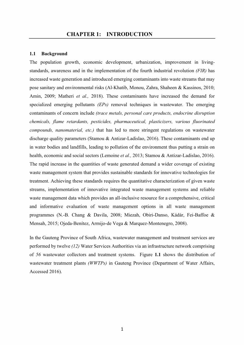
In the Gauteng Province of South Africa, wastewater management and treatment services are

performed by twelve (12) Water Services Authorities via an infrastructure network comprising

of 56 wastewater collectors and treatment systems. Figure 1.1 shows the distribution of

wastewater treatment plants (WWTPs) in Gauteng Province (Department of Water Affairs,

Accessed 2016).

2

Figure 1.1: Distribution of WWTPs in Gauteng Province, South Africa (Department of Water Affairs, Accessed 2016).

A total flow of 2579 ML/day is received at the 56 treatment facilities, which has a collective

hydraulic design capacity of 2595 ML/day (an average dry weather flow, ADWF). Gauteng

Province has some of the best wastewater practitioners’ and plants in South Africa and are

operated with non-renewable energy. These plants consistently produce high-quality effluent,

but organic and hydraulic loads exceed the theoretical design capacities (WWTPs.). To

maintain this achievement in effluent quality requires highly qualified plant managers,

adequate resources, operational adjustments and swift turnaround in scientific data collection

and analysis. Table 1.1 shows the number of WWTPs distribution in Gauteng Province, their

total design capacity in (ML/day) and total daily inflows (ML/day) (Department of Water

Affairs, Accessed 2016).

Table 1.1: Wastewater treatment plants distribution in Gauteng Province (Department of Water Affairs, Accessed 2016).

Micro Small Medium Large Macro Size Size Size Size Size Undetermined < 0.5 0.5-2 2-10. 10-25. >25 Total Ml/day Ml/day Ml/day Ml/day Ml/day Ml/day

No. of WWTPs 2 5 13 11 25 0 56

Total design capacity (Ml/day) 0.70 4.75 73.10 182 2334.50 0 2595.10

Total daily inflows (Ml/day) 0.71 3.40 59.60 131.60 2383.70 5 2576

Micro size3%

Small size9%

Medium size23%

Large size20%

Macro size45%

Distribution of WWTPs in Gauteng Province

3

South Africa adopted incentive-based regulations as a means to identify, ensure, reward, and

encourage excellence in the wastewater management (Stack, Huang, Wang & Hodge, 2011).

It is within this strategy that the Green Drop regulation programme was conceived within the

Department of Water Affairs (DWA) on the 11th September 2008, which is now referred to as

Department of Water and Sanitation (DWS). In parallel, the DWA commenced with a full-scale

assessment of all municipal WWTPs across South Africa and used this baseline to develop the

risk-based regulatory approach. This two-pronged approach by the water sector partners has

been widely acknowledged. The green drop certification incentive-based regulation seeks to

identify and develop the core competencies required for the water sector that if strengthened,

will gradually and sustainably improve the level of wastewater management in South Africa.

The risk-based regulation seeks to establish scientific baseline comprising of the critical risk

areas within the wastewater services production and to use continuous risk measurement and

reporting to ensure that corrective measures are taken to abate these high and critical risk areas

(Stack et al., 2011).

The green drop requirements are used to identify and assess the entire value chain involved in

the delivery of municipal wastewater services, whilst the risk analyses focused on the treatment

function specifically (WWTPs.). According to green drop 2009 and 2011 assessments used to

evaluate the various treatment processes applied by municipalities across the nine provinces in

South Africa, simplification of the WWTPs technology was done by grouping them into three

generic groups: (i) trickling biofilters (ii) activated sludge processes and variations and (iii)

pond and lagoon systems (Rudi & Marlene, 2013).

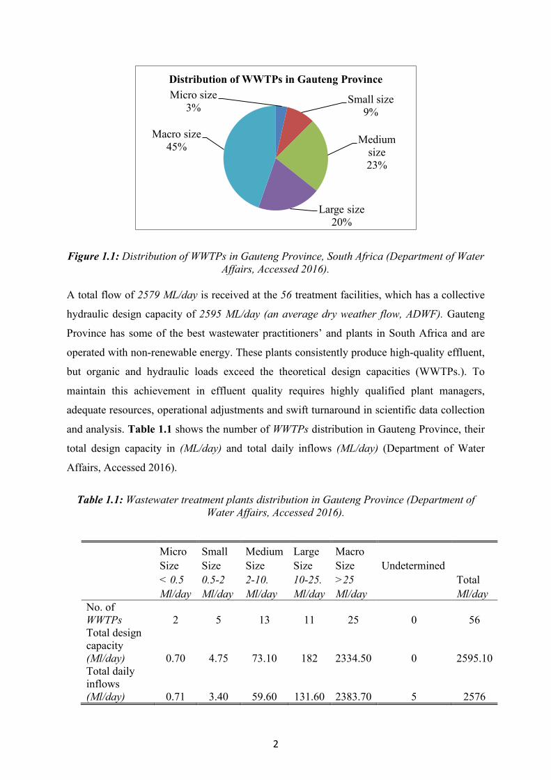
Gauteng Province has the leading numbers of wastewater treatment plants with a provincial

green drop score of 78.8%. Figure 1.2 shows the map of South Africa and Gauteng province

that serves as our research study case.

4

Figure 1.2: Gauteng province among other South African Provinces with a Provincial green drop score of 78.8%

The emerging contaminants of concern included trace metals, organics, inorganics and

micropollutants that have led to more stringent regulations on wastewater discharge quality

parameters. Wastewater treatment is inherently dynamic because of the large variation in the

influent concentration, flowrates and composition. The pollutants have attracted much attention

in recent years due to their bioaccumulation, toxicity and wide range of sources and persistence.

The presence of these pollutants is brought about by industrial activities that generate numerous

chemical elements. This creates a research gap on the construction of historical records of

contamination, quantification of the intensity of pollution based on enrichment factor, risk

assessment codes (RAC) and excess flux, and investigation of the sources by assessing inter-

elements relationships and through component analysis (Wang et al., 2015).

The automation of the wastewater treatment processes instrumentation, control and automation

(ICA) is the best approach in enhancing the efficiency of wastewater treatment process.

Developing countries still use elementary control that often fed with off-line data where the

on-line sensors that are both robust and accurate, either in-line (operating in a side stream) or

ex-situ (operating within the process), still pose major drawback and is still minimal up to date.

The is due to lack of understanding of the treatment processes and proper understanding of

mathematical models; plant constraints in flexibility to manipulate the process; lack of

fundamental knowledge concerning benefits versus costs of the automated treatment processes;

inadequate instrumentation and reliable technology; unsatisfactory communication in

designing of the plants among the designers, operators, researcher, government regulatory

agents, equipment manufacturers and suppliers and lastly lack of proper training to the

operators on how to operate the advanced sensor and control equipment (Jeppsson, 1996).

Designing and constructions of any WWTPs and selection of optimal WWTPs alternatives are

5

important issues and depends on the capital and operation cost (economic). It is provided in the

feasibility report on WWTPs project as to cut capital and operation cost (Zeng, Jiang, Huang,

Xu & Li, 2007). The development of conventional mathematical models, artificial intelligence

(AI) and optimization models in decision making has been of considerable concern over past

decade in the network design and complex interaction among various uncertain parameters

(Vahdani & Naderi-Beni, 2014). Selection of best method of treatment processes is important

before designing and implementation of programmable sampling for the cumulative risk rating

(CRR) assessment of wastewater treatment plants (Karimi, Mehrdadi, Hashemian, Bidhendi &

Moghaddam, 2011). Mathematical modelling and simulation become essential to describe,

forecast, predict and control the complicated interaction of the wastewater treatment processes

(Jeppsson, 1996). The models provide an idealized representation of an actual physical system

of the wastewater treatment system (WEF, 2011). Primary modelling allows determining

optimal working conditions which are theoretically possible to analyse and estimate the variety

of different process possibilities. This reduces additional costs for continuous and repeated

experiments. There are several computer programs that are used in the simulation modelling of

wastewater treatment processes; they include DYNOCHEM, WEST, CHEMCAD, MATLAB,

BIOWIN, WATERCAD, WEAP, STROAT, SIMBA Microsoft Excel, AI-based WWTPs

design tool and knowledge representation tool (e.g. deep learning/machine learning) in WWTP

domain among others. These programs are intended for the determination of the mass and

energy balance, and the modelling of chemical processes (Porubova, Bazbauers & Markova,

2011). Simulations by an adequate mathematical model is a novel tool for this purpose and

implementation of the mass balance models and Activated Sludge Models (ASMs) originally

proposed by the International Water Association (IWA) Task Group for mathematical

modelling of wastewater treatment processes and AI-based models are employed. The models

are validated by comparing the simulations with the laboratory experimental results and

historical big data (Henze, Gujer, Takashi & Van Loosdrecht, 2002; Parawira, 2004).

1.2 Aims and Objectives

1.2.1 Aims of the study The proposed study focused on carrying out mass balance and AI-based models of the organics,

inorganics, emerging micropollutants and trace metals on WWTPs in Gauteng province, South

Africa. The pollutants studied include trace metals (Al, As, Cd, Cr, Cu, Fe, Mn, Ni, Pb, and

Zn), total COD, filtered COD, soluble COD, (after flocculation and filtration), total nitrogen

(N), total kjeldahl nitrogen (TKN), ammonia nitrogen (NH4-N), nitrate/nitrite nitrogen, total

6

phosphorus (TP), phosphates (PO43-), volatile fatty acids (VFA), total suspended solids (TSS),

chlorine (Cl), micropollutants and trace metals.

1.2.2 Objectives of the study

The objectives of the study were:

i. To carry out site reconnaissance and dimension of the WWTPs process unit. This was

to assist in getting the complete picture (mass balance) about the occurrence,

concentration, fate and transport of trace metals, organic and inorganic compounds.

ii. To carry out in-depth sampling at different intervals (process units) based on retention

time from the liquid, mixed sludge, dewatered sludge and analyze organics, inorganics,

trace metals and emerging micropollutants.

iii. To analyse thermodynamic and reaction bio-kinetics models that will be used to gain a

better understanding of the variable dependency in the wastewater treatment process,

biosolids utilization.

iv. To carry out mathematical modelling and simulation of the trace metals, organic,

inorganic, micropollutant compounds, physically measured data (operation variables),

performance variables in the WWTPs. This will enable a better understanding of each

treatment unit and henceforth improved analytical strategies for the pollutant’s

removal.

v. To optimize parameters and validate empirical results through goodness of the

prediction (prediction performance) to ascertain comparability of satisfactory results.

7

CHAPTER 2: LITERATURE REVIEW

2.1 Introduction

This section outlines an overview of wastewater treatment plants (WWTPs in South Africa in

general and Gauteng Province in particular.

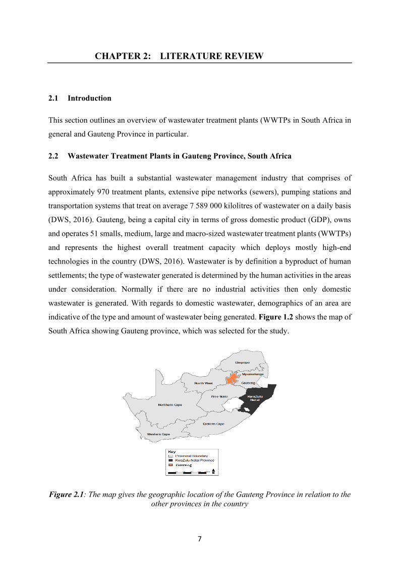
2.2 Wastewater Treatment Plants in Gauteng Province, South Africa

South Africa has built a substantial wastewater management industry that comprises of

approximately 970 treatment plants, extensive pipe networks (sewers), pumping stations and

transportation systems that treat on average 7 589 000 kilolitres of wastewater on a daily basis

(DWS, 2016). Gauteng, being a capital city in terms of gross domestic product (GDP), owns

and operates 51 smalls, medium, large and macro-sized wastewater treatment plants (WWTPs)

and represents the highest overall treatment capacity which deploys mostly high-end

technologies in the country (DWS, 2016). Wastewater is by definition a byproduct of human

settlements; the type of wastewater generated is determined by the human activities in the areas

under consideration. Normally if there are no industrial activities then only domestic

wastewater is generated. With regards to domestic wastewater, demographics of an area are

indicative of the type and amount of wastewater being generated. Figure 1.2 shows the map of

South Africa showing Gauteng province, which was selected for the study.

Figure 2.1: The map gives the geographic location of the Gauteng Province in relation to the other provinces in the country

8

The proper functioning of wastewater treatment works lies primarily with Water Service

Authorities (WSAs) and their providers (WSPs) who operate and maintain the physical

infrastructure, the chemical and biological processes. Generally, wastewater treatment plants

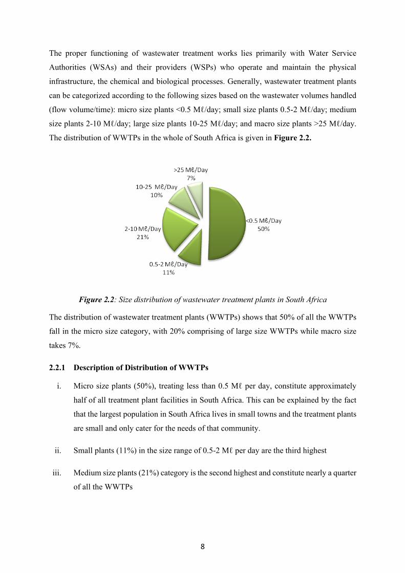
can be categorized according to the following sizes based on the wastewater volumes handled

(flow volume/time): micro size plants <0.5 Mℓ/day; small size plants 0.5-2 Mℓ/day; medium

size plants 2-10 Mℓ/day; large size plants 10-25 Mℓ/day; and macro size plants >25 Mℓ/day.

The distribution of WWTPs in the whole of South Africa is given in Figure 2.2.

Figure 2.2: Size distribution of wastewater treatment plants in South Africa

The distribution of wastewater treatment plants (WWTPs) shows that 50% of all the WWTPs

fall in the micro size category, with 20% comprising of large size WWTPs while macro size

takes 7%.

2.2.1 Description of Distribution of WWTPs

i. Micro size plants (50%), treating less than 0.5 Mℓ per day, constitute approximately

half of all treatment plant facilities in South Africa. This can be explained by the fact

that the largest population in South Africa lives in small towns and the treatment plants

are small and only cater for the needs of that community.

ii. Small plants (11%) in the size range of 0.5-2 Mℓ per day are the third highest

iii. Medium size plants (21%) category is the second highest and constitute nearly a quarter

of all the WWTPs

9

iv. Large plants (10%) category is the fourth largest of the wastewater treatment facilities

in South Africa.

v. Macro size (7%) plants >25 Mℓ/day category constitutes the smallest fraction of all the

categories of wastewater treatment facilities in South Africa. This can be understood

on the basis of the fact that the macro WWTPs are expensive to construct and maintain,

therefore can only be done in major cities like Johannesburg, Durban, Pretoria and Cape

Town.

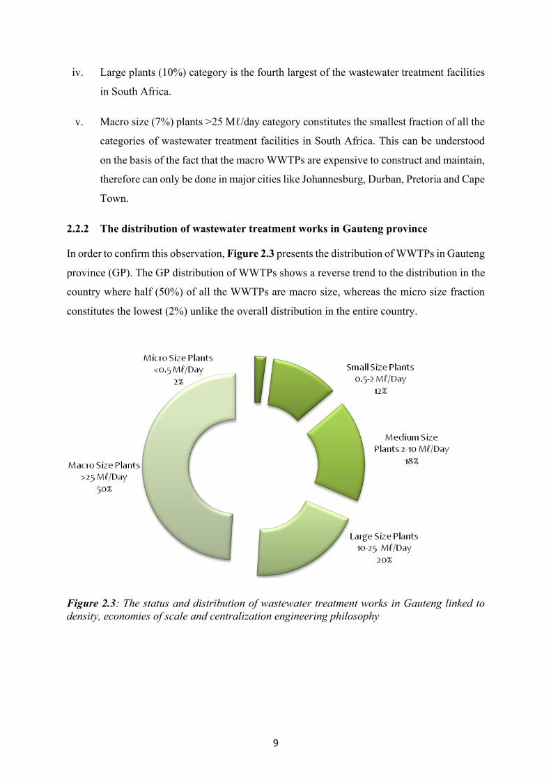
2.2.2 The distribution of wastewater treatment works in Gauteng province

In order to confirm this observation, Figure 2.3 presents the distribution of WWTPs in Gauteng

province (GP). The GP distribution of WWTPs shows a reverse trend to the distribution in the

country where half (50%) of all the WWTPs are macro size, whereas the micro size fraction

constitutes the lowest (2%) unlike the overall distribution in the entire country.

Figure 2.3: The status and distribution of wastewater treatment works in Gauteng linked to density, economies of scale and centralization engineering philosophy

10

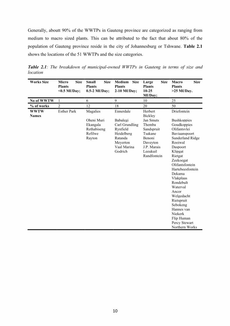
Generally, aboutt 90% of the WWTPs in Gauteng province are categorized as ranging from

medium to macro sized plants. This can be attributed to the fact that about 80% of the

population of Gauteng province reside in the city of Johannesburg or Tshwane. Table 2.1

shows the locations of the 51 WWTPs and the size categories.

Table 2.1: The breakdown of municipal-owned WWTPs in Gauteng in terms of size and location

Works Size Micro Size Plants <0.5 Mℓ/Day;

Small Size Plants 0.5-2 Mℓ/Day;

Medium Size Plants 2-10 Mℓ/Day;

Large Size Plants 10-25 Mℓ/Day;

Macro Size Plants >25 Mℓ/Day.

No of WWTW 1 6 9 10 25 % of works 2 12 18 20 50 WWTW Names

Esther Park Magalies Ennerdale Herbert Bickley

Driefontein

Oheni Muri Babalegi Jan Smuts Bushkoppies Ekangala Carl Grundling Themba Goudkoppies Rethabiseng Rynfield Sandspruit Olifantsvlei Refilwe Heidelberg Tsakane Baviaanspoort Rayton Ratanda Benoni Sunderland Ridge Meyerton Daveyton Rooiwal Vaal Marina J.P. Marais Daspoort Godrich Leeukuil Klipgat Randfontein Rietgat Zeekoegat Olifantsfontein Hartebeesfontein Dekama Vlakplaas Rondebult Waterval Ancor Welgedacht Rietspruit Sebokeng Hannes van

Niekerk Flip Human Percy Stewart Northern Works

11

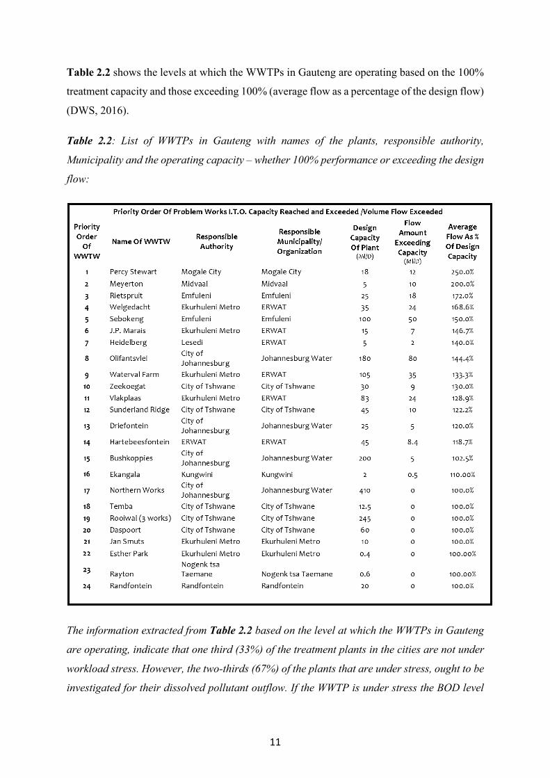
Table 2.2 shows the levels at which the WWTPs in Gauteng are operating based on the 100%

treatment capacity and those exceeding 100% (average flow as a percentage of the design flow)

(DWS, 2016).

Table 2.2: List of WWTPs in Gauteng with names of the plants, responsible authority,

Municipality and the operating capacity – whether 100% performance or exceeding the design

flow:

The information extracted from Table 2.2 based on the level at which the WWTPs in Gauteng

are operating, indicate that one third (33%) of the treatment plants in the cities are not under

workload stress. However, the two-thirds (67%) of the plants that are under stress, ought to be

investigated for their dissolved pollutant outflow. If the WWTP is under stress the BOD level

12

will be high and this might pose a challenge in the mobilization of heavy metals bound on

humic and fulvic acids.

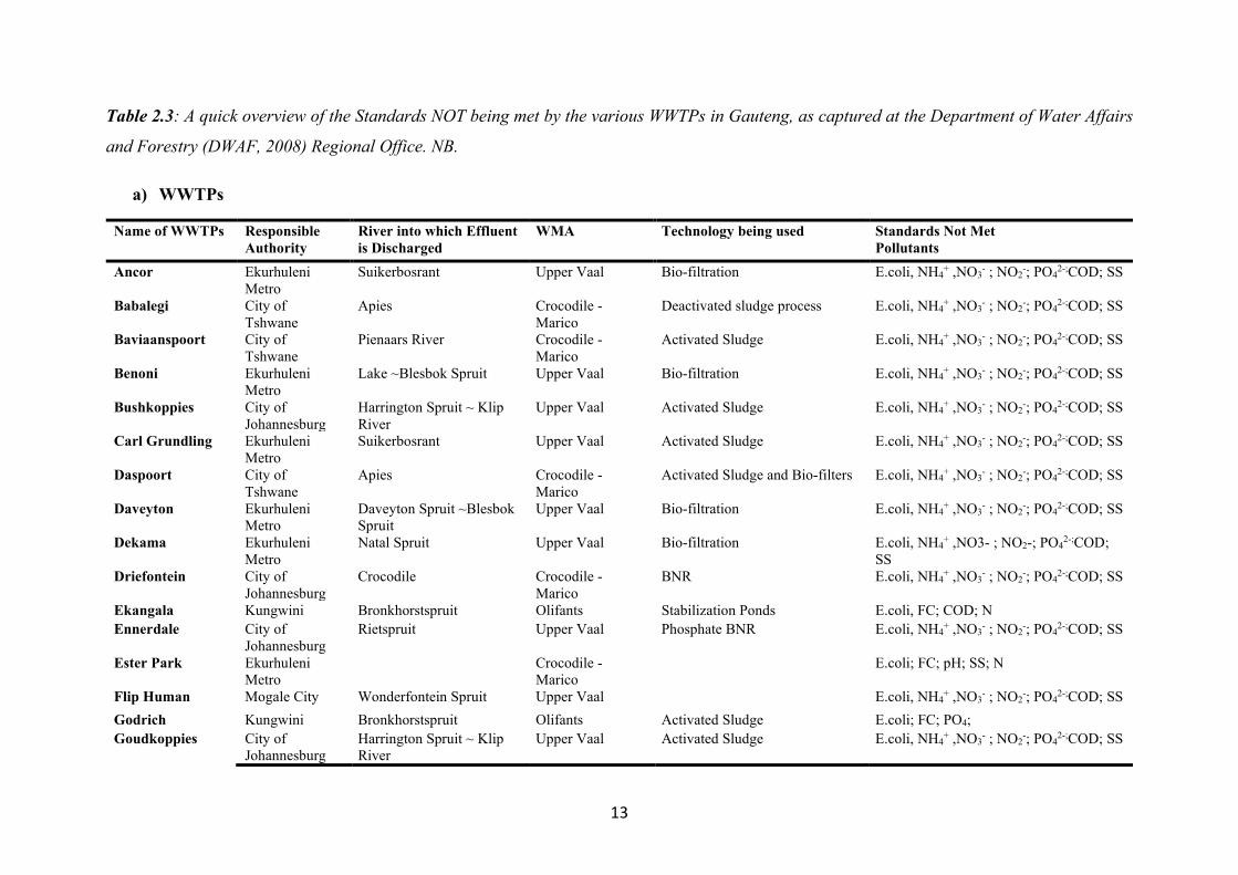
Table 2.3 is an overview of the Standards NOT being met by the various WWTPs in Gauteng,

as captured by the Department of Water and Sanitation (DWS, 2016) Regional Office (now

known as Department of Water & Sanitation).

13

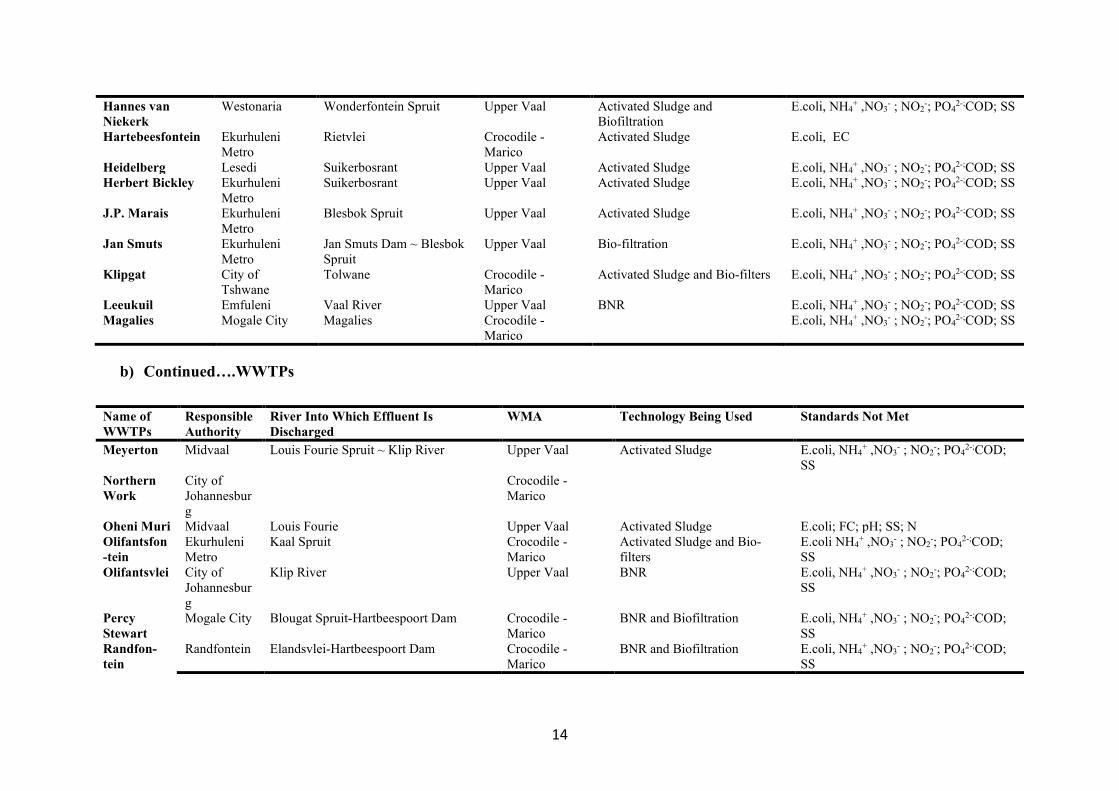
Table 2.3: A quick overview of the Standards NOT being met by the various WWTPs in Gauteng, as captured at the Department of Water Affairs

and Forestry (DWAF, 2008) Regional Office. NB.

a) WWTPs

Name of WWTPs Responsible Authority

River into which Effluent is Discharged

WMA Technology being used Standards Not Met Pollutants

Ancor Ekurhuleni Metro

Suikerbosrant Upper Vaal Bio-filtration E.coli, NH4+ ,NO3

- ; NO2-; PO4

2-;COD; SS

Babalegi City of Tshwane

Apies Crocodile - Marico

Deactivated sludge process E.coli, NH4+ ,NO3

- ; NO2-; PO4

2-;COD; SS

Baviaanspoort City of Tshwane

Pienaars River Crocodile - Marico

Activated Sludge E.coli, NH4+ ,NO3

- ; NO2-; PO4

2-;COD; SS

Benoni Ekurhuleni Metro

Lake ~Blesbok Spruit Upper Vaal Bio-filtration E.coli, NH4+ ,NO3

- ; NO2-; PO4

2-;COD; SS

Bushkoppies City of Johannesburg

Harrington Spruit ~ Klip River

Upper Vaal Activated Sludge E.coli, NH4+ ,NO3

- ; NO2-; PO4

2-;COD; SS

Carl Grundling Ekurhuleni Metro

Suikerbosrant Upper Vaal Activated Sludge E.coli, NH4+ ,NO3

- ; NO2-; PO4

2-;COD; SS

Daspoort City of Tshwane


Activated Sludge and Bio-filters E.coli, NH4+ ,NO3

- ; NO2-; PO4

2-;COD; SS

Daveyton Ekurhuleni Metro

Daveyton Spruit ~Blesbok Spruit

Upper Vaal Bio-filtration E.coli, NH4+ ,NO3

- ; NO2-; PO4

2-;COD; SS

Dekama Ekurhuleni Metro

Natal Spruit Upper Vaal Bio-filtration E.coli, NH4+ ,NO3- ; NO2-; PO4

2-;COD; SS

Driefontein City of Johannesburg

Crocodile Crocodile - Marico

BNR E.coli, NH4+ ,NO3

- ; NO2-; PO4

2-;COD; SS

Ekangala Kungwini Bronkhorstspruit Olifants Stabilization Ponds E.coli, FC; COD; N Ennerdale City of

Johannesburg Rietspruit Upper Vaal Phosphate BNR E.coli, NH4

+ ,NO3- ; NO2

-; PO42-;COD; SS

Ester Park Ekurhuleni Metro

Crocodile - Marico

E.coli; FC; pH; SS; N

Flip Human Mogale City Wonderfontein Spruit Upper Vaal E.coli, NH4+ ,NO3

- ; NO2-; PO4

2-;COD; SS Godrich Kungwini Bronkhorstspruit Olifants Activated Sludge E.coli; FC; PO4; Goudkoppies City of

Johannesburg Harrington Spruit ~ Klip River

Upper Vaal Activated Sludge E.coli, NH4+ ,NO3

- ; NO2-; PO4

2-;COD; SS

14

Hannes van Niekerk

Westonaria Wonderfontein Spruit Upper Vaal Activated Sludge and Biofiltration

E.coli, NH4+ ,NO3

- ; NO2-; PO4

2-;COD; SS

Hartebeesfontein Ekurhuleni Metro

Rietvlei Crocodile - Marico

Activated Sludge E.coli, EC

Heidelberg Lesedi Suikerbosrant Upper Vaal Activated Sludge E.coli, NH4+ ,NO3

- ; NO2-; PO4

2-;COD; SS Herbert Bickley Ekurhuleni

Metro Suikerbosrant Upper Vaal Activated Sludge E.coli, NH4

+ ,NO3- ; NO2

-; PO42-;COD; SS

J.P. Marais Ekurhuleni Metro

Blesbok Spruit Upper Vaal Activated Sludge E.coli, NH4+ ,NO3

- ; NO2-; PO4

2-;COD; SS

Jan Smuts Ekurhuleni Metro

Jan Smuts Dam ~ Blesbok Spruit

Upper Vaal Bio-filtration E.coli, NH4+ ,NO3

- ; NO2-; PO4

2-;COD; SS

Klipgat City of Tshwane

Tolwane Crocodile - Marico

Activated Sludge and Bio-filters E.coli, NH4+ ,NO3

- ; NO2-; PO4

2-;COD; SS

Leeukuil Emfuleni Vaal River Upper Vaal BNR E.coli, NH4+ ,NO3

- ; NO2-; PO4

2-;COD; SS Magalies Mogale City Magalies Crocodile -

Marico E.coli, NH4

+ ,NO3- ; NO2

-; PO42-;COD; SS

b) Continued….WWTPs

Name of WWTPs

Responsible Authority

River Into Which Effluent Is Discharged

WMA Technology Being Used Standards Not Met

Meyerton Midvaal Louis Fourie Spruit ~ Klip River Upper Vaal Activated Sludge E.coli, NH4+ ,NO3

- ; NO2-; PO4

2-;COD; SS

Northern Work

City of Johannesburg

Crocodile - Marico

Oheni Muri Midvaal Louis Fourie Upper Vaal Activated Sludge E.coli; FC; pH; SS; N Olifantsfon-tein

Ekurhuleni Metro

Kaal Spruit Crocodile - Marico

Activated Sludge and Bio-filters

E.coli NH4+ ,NO3

- ; NO2-; PO4

2-;COD; SS

Olifantsvlei City of Johannesburg

Klip River Upper Vaal BNR E.coli, NH4+ ,NO3

- ; NO2-; PO4

2-;COD; SS

Percy Stewart

Mogale City Blougat Spruit-Hartbeespoort Dam Crocodile - Marico

BNR and Biofiltration E.coli, NH4+ ,NO3

- ; NO2-; PO4

2-;COD; SS

Randfon-tein

Randfontein Elandsvlei-Hartbeespoort Dam Crocodile - Marico

BNR and Biofiltration E.coli, NH4+ ,NO3

- ; NO2-; PO4

2-;COD; SS

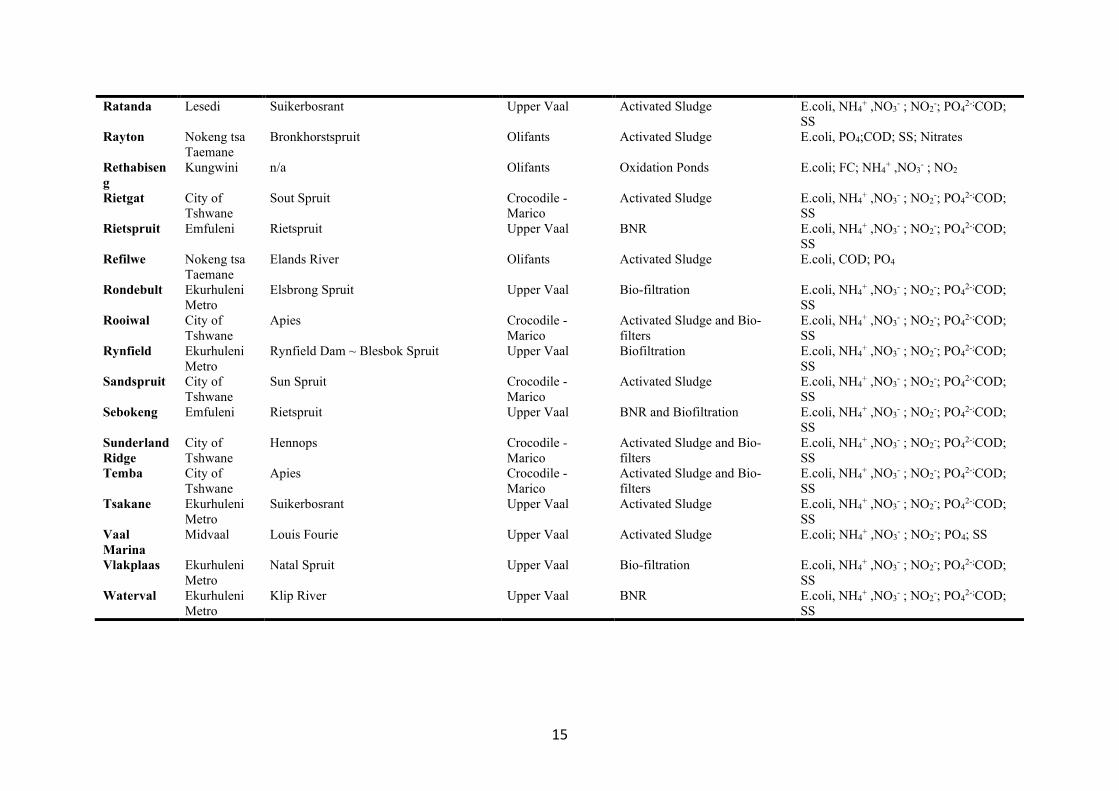
15

Ratanda Lesedi Suikerbosrant Upper Vaal Activated Sludge E.coli, NH4+ ,NO3

- ; NO2-; PO4

2-;COD; SS

Rayton Nokeng tsa Taemane

Bronkhorstspruit Olifants Activated Sludge E.coli, PO4;COD; SS; Nitrates

Rethabiseng

Kungwini n/a Olifants Oxidation Ponds E.coli; FC; NH4+ ,NO3

- ; NO2

Rietgat City of Tshwane

Sout Spruit Crocodile - Marico


- ; NO2-; PO4

2-;COD; SS

Rietspruit Emfuleni Rietspruit Upper Vaal BNR E.coli, NH4+ ,NO3

- ; NO2-; PO4

2-;COD; SS

Refilwe Nokeng tsa Taemane

Elands River Olifants Activated Sludge E.coli, COD; PO4

Rondebult Ekurhuleni Metro

Elsbrong Spruit Upper Vaal Bio-filtration E.coli, NH4+ ,NO3

- ; NO2-; PO4

2-;COD; SS

Rooiwal City of Tshwane



E.coli, NH4+ ,NO3

- ; NO2-; PO4

2-;COD; SS

Rynfield Ekurhuleni Metro

Rynfield Dam ~ Blesbok Spruit Upper Vaal Biofiltration E.coli, NH4+ ,NO3

- ; NO2-; PO4

2-;COD; SS

Sandspruit City of Tshwane

Sun Spruit Crocodile - Marico


- ; NO2-; PO4

2-;COD; SS

Sebokeng Emfuleni Rietspruit Upper Vaal BNR and Biofiltration E.coli, NH4+ ,NO3

- ; NO2-; PO4

2-;COD; SS

Sunderland Ridge

City of Tshwane

Hennops Crocodile - Marico


E.coli, NH4+ ,NO3

- ; NO2-; PO4

2-;COD; SS

Temba City of Tshwane



E.coli, NH4+ ,NO3

- ; NO2-; PO4

2-;COD; SS

Tsakane Ekurhuleni Metro

Suikerbosrant Upper Vaal Activated Sludge E.coli, NH4+ ,NO3

- ; NO2-; PO4

2-;COD; SS

Vaal Marina

Midvaal Louis Fourie Upper Vaal Activated Sludge E.coli; NH4+ ,NO3

- ; NO2-; PO4; SS

Vlakplaas Ekurhuleni Metro

Natal Spruit Upper Vaal Bio-filtration E.coli, NH4+ ,NO3

- ; NO2-; PO4

2-;COD; SS

Waterval Ekurhuleni Metro

Klip River Upper Vaal BNR E.coli, NH4+ ,NO3

- ; NO2-; PO4

2-;COD; SS

16

2.3 Wastewater Treatment Processes

Wastewater collected from cities and towns must ultimately be returned to receiving water or

to the land. The complex question that seeks to be answered relate to the nature and the extent

to which contaminants in wastewater must be removed to protect the environment. These

questions must be answered specifically for each case. This requires analyses of local

conditions and terms of reference, together with application of scientific knowledge,

engineering judgment consideration of the South Africa National Standards (SANS) or World

Health Organization (WHO) (Health.).

2.3.1 Components of wastewater treatment plants

The components that make up the wastewater flow from any community depends on the

following factors (E. Metcalf).

• Domestics (sanitary) wastewater, this is the wastewater discharged from residential,

commercial and institutional facilities.

• Industrial wastewater, this is wastewater discharge from the industry.

• Infiltration/inflow, this is the storm water that enters the sewer either indirectly or

directly. Infiltration is water that enters the sewer system through leaking joints, cracks

and breaks, or porous walls. Inflow is storm water that enters the sewer system from

storm drain connections (catch basins), roof leaders, foundation and basement drains,

or through manhole covers.

• Storm water, rainwater and snowmelt runoff.

2.3.2 Classification of treatment methods

The principal methods used for the treatment of wastewater and sludge are identified in Figure

2.4 where unit operations and processes are grouped together to provide various levels of

treatments. The term “preliminary” or “primary”, refers to physical unit operations,

“secondary” refers to chemical and biological unit processes, and “advanced” or “tertiary”

refers to combination of all three. The major stages in wastewater treatment plants and the unit

operations, processes or methods applicable to the removal of these contaminants, are shown

in Figure 2.4 (E. Metcalf).

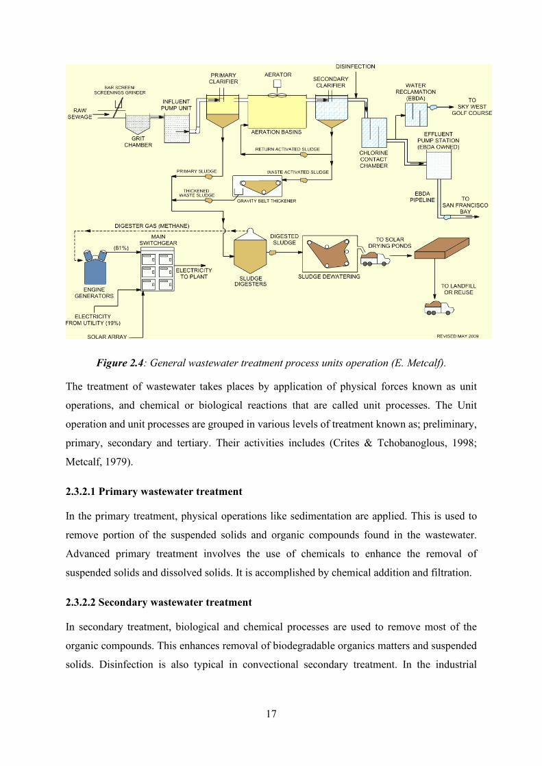
17

Figure 2.4: General wastewater treatment process units operation (E. Metcalf).

The treatment of wastewater takes places by application of physical forces known as unit

operations, and chemical or biological reactions that are called unit processes. The Unit

operation and unit processes are grouped in various levels of treatment known as; preliminary,

primary, secondary and tertiary. Their activities includes (Crites & Tchobanoglous, 1998;

Metcalf, 1979).

2.3.2.1 Primary wastewater treatment

In the primary treatment, physical operations like sedimentation are applied. This is used to

remove portion of the suspended solids and organic compounds found in the wastewater.

Advanced primary treatment involves the use of chemicals to enhance the removal of

suspended solids and dissolved solids. It is accomplished by chemical addition and filtration.

2.3.2.2 Secondary wastewater treatment

In secondary treatment, biological and chemical processes are used to remove most of the

organic compounds. This enhances removal of biodegradable organics matters and suspended

solids. Disinfection is also typical in convectional secondary treatment. In the industrial

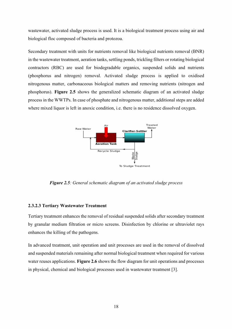
18

wastewater, activated sludge process is used. It is a biological treatment process using air and

biological floc composed of bacteria and protozoa.

Secondary treatment with units for nutrients removal like biological nutrients removal (BNR)

in the wastewater treatment, aeration tanks, settling ponds, trickling filters or rotating biological

contractors (RBC) are used for biodegradable organics, suspended solids and nutrients

(phosphorus and nitrogen) removal. Activated sludge process is applied to oxidised

nitrogenous matter, carbonaceous biological matters and removing nutrients (nitrogen and

phosphorus). Figure 2.5 shows the generalized schematic diagram of an activated sludge

process in the WWTPs. In case of phosphate and nitrogenous matter, additional steps are added

where mixed liquor is left in anoxic condition, i.e. there is no residence dissolved oxygen.

Figure 2.5: General schematic diagram of an activated sludge process

2.3.2.3 Tertiary Wastewater Treatment

Tertiary treatment enhances the removal of residual suspended solids after secondary treatment

by granular medium filtration or micro screens. Disinfection by chlorine or ultraviolet rays

enhances the killing of the pathogens.

In advanced treatment, unit operation and unit processes are used in the removal of dissolved

and suspended materials remaining after normal biological treatment when required for various

water reuses applications. Figure 2.6 shows the flow diagram for unit operations and processes

in physical, chemical and biological processes used in wastewater treatment [3].

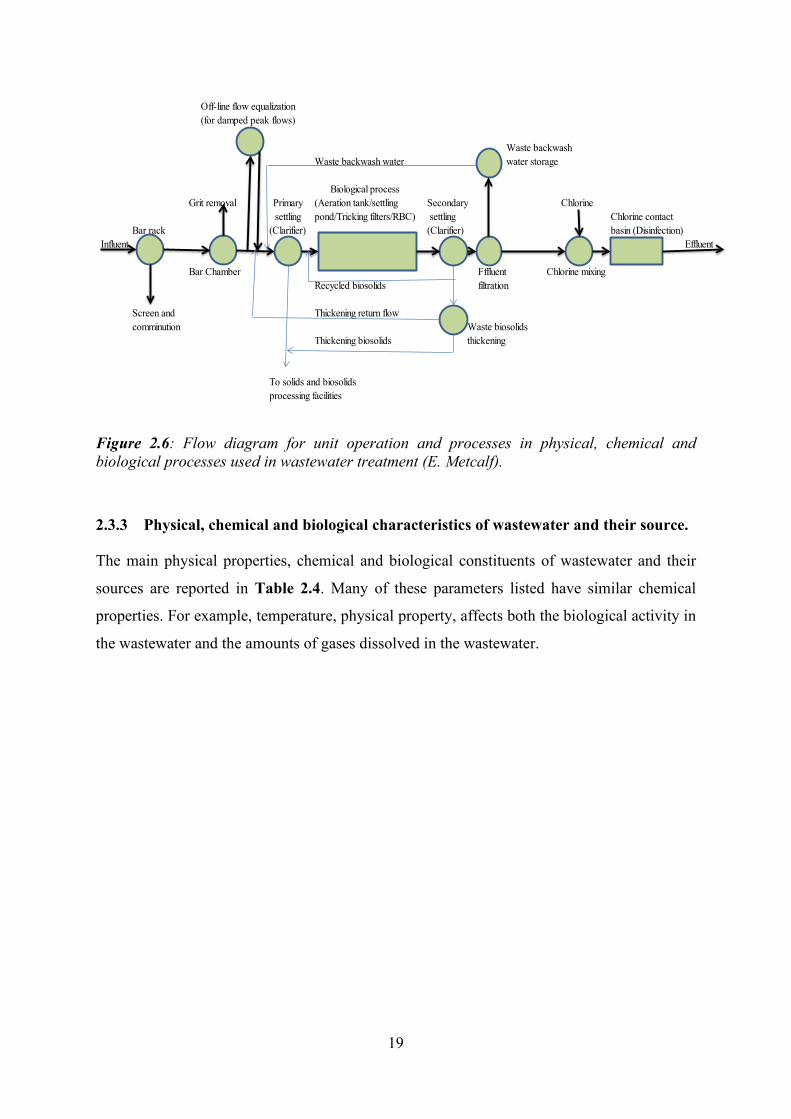
19

Figure 2.6: Flow diagram for unit operation and processes in physical, chemical and biological processes used in wastewater treatment (E. Metcalf).

2.3.3 Physical, chemical and biological characteristics of wastewater and their source.

The main physical properties, chemical and biological constituents of wastewater and their

sources are reported in Table 2.4. Many of these parameters listed have similar chemical

properties. For example, temperature, physical property, affects both the biological activity in

the wastewater and the amounts of gases dissolved in the wastewater.

Off-line flow equalization(for damped peak flows)

Waste backwashWaste backwash water water storage

Primary (Aeration tank/settling Secondarysettling pond/Tricking filters/RBC) settling Chlorine contact

Bar rack (Clarifier) (Clarifier) basin (Disinfection)Influent Effluent

Bar Chamber Fffluent Chlorine mixingRecycled biosolids filtration

Screen and Thickening return flowcomminution Waste biosolids

Thickening biosolids thickening

To solids and biosolids processing facilities

Grit removalBiological process

Chlorine

20

Table 2.4: Important contaminants of concern in wastewater treatment (Henze & Comeau,

2008; Metcalf, 1979)

Contaminants Reason for importance

Suspended solids Suspended solids can lead to the development of sludge deposits and anaerobic conditions when untreated wastewater is discharged in the aquatic environment

Biodegradable organics

Composed principally of proteins, carbohydrates and fats, biodegradable organics are measured most commonly in terms of BOD (Biochemical Oxygen Demand) and COD (Chemical Oxygen Demand). If untreated and discharged to the environment, their biological stabilization can lead to the depletion of the natural oxygen resources and to the development of septic condition.

Pathogens Communicable diseases can be transmitted but the pathogenic organisms in wastewater

Nutrients Both nitrogen and phosphorus, along with carbon are essential nutrients for growth. When discharged to the aquatic environment, these nutrients can lead to the growth of undesirable aquatics life thus leading to pollution of groundwater

Priority pollutants Organics and inorganics compounds selected on the basis on their known or suspected carcinogenicity, mutagenicity, teratogenicity, or high acute toxicity.

Refractory organics These organics tends to resist conventional methods of wastewater treatment. Typical examples include surfactants, phenols and agricultural pesticides

Heavy metals Heavy metals are usually added to wastewater from commercial and industrial activities and may have to be removed if the wastewater is to be reused

Dissolved inorganics Inorganics constituents such as calcium, sodium and sulphate are added to the original domestic’s water supply as a results of water use and may have to be removed if the wastewater is to be reused.

2.3.3.1 The quantitative methods of analysis: gravimetric, volumetric or physicochemical.

Analysis of the contaminants listed in Table 2.4 required different analytical methods

depending on the nature of the contaminant, the availability of the technique and the

information required.

• Physiochemical methods of analysis include; turbidity, calorimetry, potentiometry,

polarography, fluorometry, spectroscopy and nuclear radiation.

• Volumetric methods are based on; analysis volumes, e.g. flow rate of the wastewater.

• Gravimetric methods are based on; analysis mass of mass, e.g. methods to determine

suspended solids (E. Metcalf).

2.4 Mechanisms of the Treatment Processes

Different mechanisms or pollutant removal methods are available. These discussed below.

21

2.4.1 Sedimentation

Sedimentation is more or less effective for the removal of suspended matter, depending upon

the size and the density of the particles to be removed and time available for the process. Heavy

and large particles are removed in a relatively short time, while much light or finely divided

material takes longer period, e.g. clay soils. If the concentration of such “non-settleable”

particles is excessive, then sedimentation alone is not an adequate method of treatment, and

other means are employed (Metcalf, 1979).

2.4.2 Coagulation

This is a technique of treating water with certain chemicals for the purpose of collecting non-

settleable particles into larger or heavier aggregates which are more readily removed. The

resulting clumps of solids material, termed “floc” are removed by sedimentation, filtration, or

both. Optimum amount of chemicals are used in coagulation processes (Metcalf, 1979).

2.4.3 Filtration

This process in capable of removing particulate matters too light or too finely divided to be

removed by sedimentation. That is, sand, anthracite, diatomite and other fine-grained materials.

Filtration always follows sedimentation units, so that the larger quantity of relatively coarse

material is removed by sedimentation, to avoid rapid clogging of the filter, which in turn

remove the particles for which sedimentation is not effective. Fine screens or micro-strainers

are sometimes used prior to sand filtration (Metcalf, 1979).

2.4.4 Disinfection

Disinfection is conducted in order to destroy pathogenic organisms. It is usually accomplished

by the application of chlorine or certain chlorine compounds. Other methods using ultra violet

rays and ozonation are also currently in use. Disinfection is the only step which is intended

specifically for control of the bacteriological quality (Metcalf, 1979).

2.4.5 Softening

The removal of the elements which contribute to hardness of a water, primarily calcium and

magnesium, is called softening. When domestic supplies are softened, usually the lime-soda

process or the ion-exchange process, is used. Chemicals are added to precipitate calcium

carbonate, and if further softening is required, magnesium is precipitated as magnesium

hydroxide. Usually, the process results in a reduction of the total quantity of dissolved solids

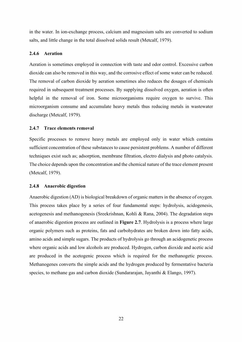
22

in the water. In ion-exchange process, calcium and magnesium salts are converted to sodium

salts, and little change in the total dissolved solids result (Metcalf, 1979).

2.4.6 Aeration

Aeration is sometimes employed in connection with taste and odor control. Excessive carbon

dioxide can also be removed in this way, and the corrosive effect of some water can be reduced.

The removal of carbon dioxide by aeration sometimes also reduces the dosages of chemicals

required in subsequent treatment processes. By supplying dissolved oxygen, aeration is often

helpful in the removal of iron. Some microorganisms require oxygen to survive. This

microorganism consume and accumulate heavy metals thus reducing metals in wastewater

discharge (Metcalf, 1979).

2.4.7 Trace elements removal

Specific processes to remove heavy metals are employed only in water which contains

sufficient concentration of these substances to cause persistent problems. A number of different

techniques exist such as; adsorption, membrane filtration, electro dialysis and photo catalysis.

The choice depends upon the concentration and the chemical nature of the trace element present

(Metcalf, 1979).

2.4.8 Anaerobic digestion

Anaerobic digestion (AD) is biological breakdown of organic matters in the absence of oxygen.

This process takes place by a series of four fundamental steps: hydrolysis, acidogenesis,

acetogenesis and methanogenesis (Sreekrishnan, Kohli & Rana, 2004). The degradation steps

of anaerobic digestion process are outlined in Figure 2.7. Hydrolysis is a process where large

organic polymers such as proteins, fats and carbohydrates are broken down into fatty acids,

amino acids and simple sugars. The products of hydrolysis go through an acidogenetic process

where organic acids and low alcohols are produced. Hydrogen, carbon dioxide and acetic acid

are produced in the acetogenic process which is required for the methanogetic process.

Methanogenes converts the simple acids and the hydrogen produced by fermentative bacteria

species, to methane gas and carbon dioxide (Sundararajan, Jayanthi & Elango, 1997).

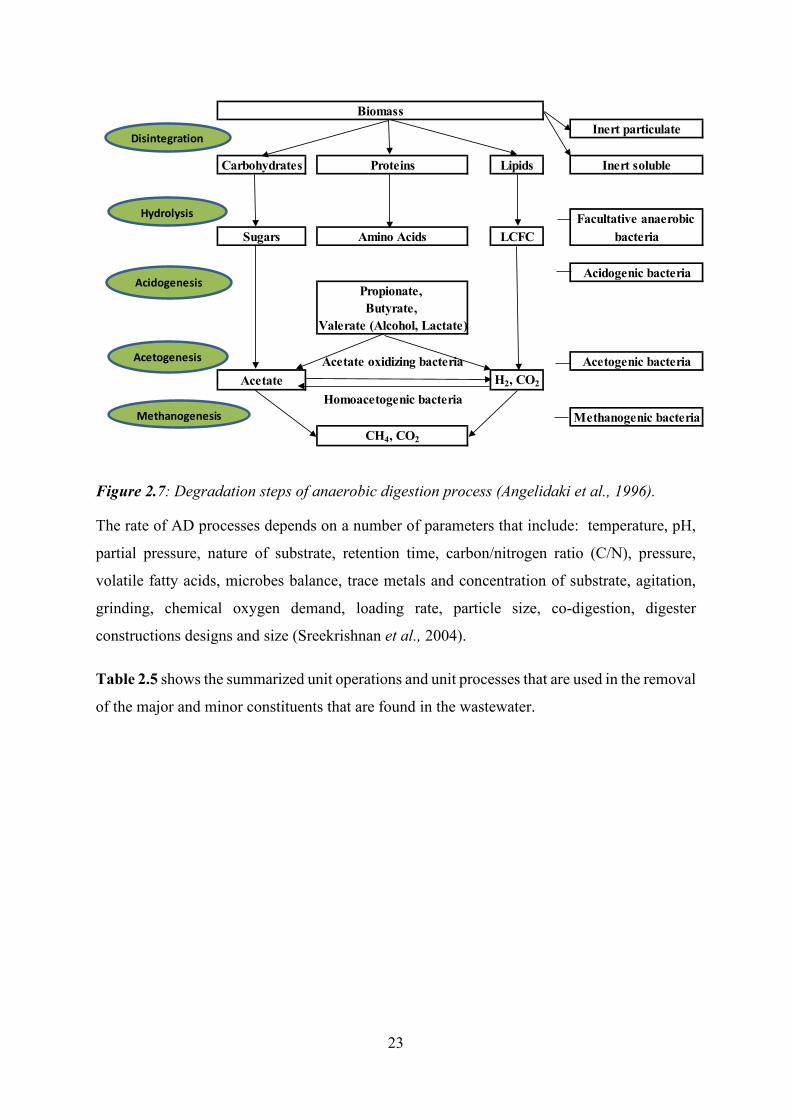
23

Figure 2.7: Degradation steps of anaerobic digestion process (Angelidaki et al., 1996).

The rate of AD processes depends on a number of parameters that include: temperature, pH,

partial pressure, nature of substrate, retention time, carbon/nitrogen ratio (C/N), pressure,

volatile fatty acids, microbes balance, trace metals and concentration of substrate, agitation,

grinding, chemical oxygen demand, loading rate, particle size, co-digestion, digester

constructions designs and size (Sreekrishnan et al., 2004).

Table 2.5 shows the summarized unit operations and unit processes that are used in the removal

of the major and minor constituents that are found in the wastewater.

Inert particulate

Carbohydrates Proteins Lipids Inert soluble

Facultative anaerobic Sugars Amino Acids LCFC bacteria

Acidogenic bacteriaPropionate, Butyrate,

Valerate (Alcohol, Lactate)

Acetate oxidizing bacteria Acetogenic bacteriaAcetate H2, CO2

Homoacetogenic bacteriaMethanogenic bacteria

CH4, CO2

Biomass

Hydrolysis

Acidogenesis

Acetogenesis

Methanogenesis

Disintegration

24

Table 2.5: Unit operation and processes in wastewater treatment plants (E. Metcalf)

Constituent Unit operation or process Suspended solids Screening Grit removal Sedimentation High-rate clarification Flotation Chemical precipitation Depth filtration Surface filtration Biodegradable organics Aerobic attached growth variation Aerobic suspended growth variation Anaerobic suspended growth variation Anaerobic attached growth variation Lagoon variation Physical-chemical systems Chemical oxidation Membrane filtration Phosphorus Chemical treatment Biological phosphorus removal Nitrogen Chemical oxidation (breakpoint chlorination) Suspended-growth/Fixed-film nitrification and denitrification variation Air stripping Ion exchange Nitrogen and Phosphorus Biological nutrients removal variations Pathogens Chlorine dioxide Chlorine compounds Ozone Ultraviolet (UV) radiation Colloidal and dissolved solids Membranes Carbon adsorption Ion exchange Chemical treatment Volatile organic compounds Air stripping Carbon adsorption Advanced oxidation Odors Carbon adsorption Chemical scrubbers Bio-filters

Compost filters

25

2.5 Technique used in Selecting Plants to Sample

Several methods have been developed to give unbiased results when it comes to decision

making on a choice of technology. In principle, all methods are based on the steps summarized

below (Kigozi, Aboyade & Muzenda, 2014);

• Identification of the problem

• Identification of stakeholders

• Seeking the unbiased opinions of the stakeholders in the form of solutions to the

identified problem. The identified solutions are treated as alternatives and the key

performance indicators of the chosen options become the selection criteria

• Modelling the obtained solutions so as to obtain impartial results through detailed

analyses. At the modelling stage is when the decision maker decides on which particular

selection method to employ basing on the nature of the problem at hand.

In modern times, technologies are probabilistic in nature and the evaluation criterion are multi-

dimensional. This calls for complex tools that can capture all the dimensions of a decision

problem. The existing technology selection methods include;

2.5.1 Multi-criteria decision analysis (MCDA)

Multi-criteria decision analysis (MCDA) is an approach employed by decision makers to make

recommendations from a set of finite seemingly similar options based on how well they score

against a pre-defined set of criteria. MCDA techniques aim to achieve a decision goal from a

set of alternatives using pre-set selection factors herein referred to as the criteria (Chai, Liu &

Ngai, 2013). The selection criteria are assigned weights by the decision maker basing on their

level of importance. Then using appropriate techniques, the alternatives are awarded scores

depending on how well they perform with regard to particular criteria. Finally ranks of

alternatives are computed as an aggregate sum of products of the alternatives with

corresponding criteria. From the ranking, a decision is then made (Dodgson, Spackman,

Pearman & Phillips, 2009).

There are several variations in MCDA techniques used currently employing mathematics and

psychology. These include; analytic hierarchy process (AHP), Simple multi-attribute rating

technique (SMART) and case-based reasoning (CBR).

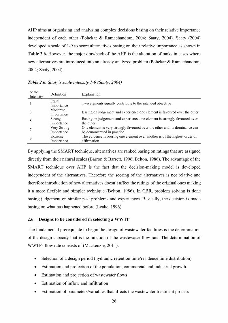
26

AHP aims at organizing and analyzing complex decisions basing on their relative importance

independent of each other (Pohekar & Ramachandran, 2004; Saaty, 2004). Saaty (2004)

developed a scale of 1-9 to score alternatives basing on their relative importance as shown in

Table 2.6. However, the major drawback of the AHP is the alteration of ranks in cases where

new alternatives are introduced into an already analyzed problem (Pohekar & Ramachandran,

2004; Saaty, 2004).

Table 2.6: Saaty’s scale intensity 1-9 (Saaty, 2004)

Scale Intensity Definition Explanation

1 Equal Importance Two elements equally contribute to the intended objective

3 Moderate importance Basing on judgement and experience one element is favoured over the other

5 Strong Importance

Basing on judgement and experience one element is strongly favoured over the other

7 Very Strong Importance

One element is very strongly favoured over the other and its dominance can be demonstrated in practice

9 Extreme Importance

The evidence favouring one element over another is of the highest order of affirmation

By applying the SMART technique, alternatives are ranked basing on ratings that are assigned

directly from their natural scales (Barron & Barrett, 1996; Belton, 1986). The advantage of the

SMART technique over AHP is the fact that the decision-making model is developed

independent of the alternatives. Therefore the scoring of the alternatives is not relative and

therefore introduction of new alternatives doesn’t affect the ratings of the original ones making

it a more flexible and simpler technique (Belton, 1986). In CBR, problem solving is done

basing judgement on similar past problems and experiences. Basically, the decision is made

basing on what has happened before (Leake, 1996).

2.6 Designs to be considered in selecting a WWTP

The fundamental prerequisite to begin the design of wastewater facilities is the determination

of the design capacity that is the function of the wastewater flow rate. The determination of

WWTPs flow rate consists of (Mackenzie, 2011):

• Selection of a design period (hydraulic retention time/residence time distribution)

• Estimation and projection of the population, commercial and industrial growth.

• Estimation and projection of wastewater flows

• Estimation of inflow and infiltration

• Estimation of parameters/variables that affects the wastewater treatment process

27

2.6.1 Establishment of design criteria

The design criteria for the construction of wastewater treatment consists of performance. This

establishes the functional performance of the plant. The design criterion is the combination of

the two. Performance criteria defines the desired objective but eliminates means of achieving

this (Mackenzie, 2011).

The factors to be considered in establishing the design criteria for the water and wastewater

treatment systems include:

• Environmental and regulatory standards

• Wastewater characteristics

• Site limits

• System reliability

• Design life

• Cost

2.6.2 Environmental and regulatory

The standards are prescribed by the regulating agency under the Law. This provides the basis

for elimination of treatment technologies that are not appropriate. The standards require that

WWTPs meets performance standards/numerical requirements for organic compounds and

trace elements concentration. Modeling can assist WWTPs in meeting the required standards.

The Agency do not prescribe the technology that is to be used in meeting the standards but set

goals to be achieved by the engineers when selecting the appropriate treatment processes

(Mackenzie, 2011).

2.6.3 Wastewater characteristics

Wastewater characteristics include the flow rate of the wastewater and its composition. The

wastewater characteristics include (Mackenzie, 2011):

• Contribution from commercial and industrial activity.

• Composition and strength of the wastewater

• Hourly, daily, weekly, monthly, and seasonal variations in flows and strength of the

wastewater

• Rainfall/runoff intrusion

28

2.6.4 System reliability

System reliability refers to the ability of a component or system to perform its designated

function without failure.

2.6.5 Site limitation

The area and location available for the treatment plant, sewer systems, and water distribution

system availability of roads, power, and a connection to the raw water supply define the site

limits.

2.6.6 Design life

Design life is the economic comparison of alternatives (components of processes with different

designs).

2.6.7 Cost

Design criteria for the process units and manpower depend on the economics evaluation. This

cost estimates consist of capital costs (construction, engineering, land, legal, and

administrative) and operating cost (personal, power, chemical, miscellaneous utilities). The

economic analysis includes; present worth, annual cash flow, rate of return, benefits-cost and

breakeven analysis.

2.7 Classification of WWTPs according to nature of influent

Wastewater is classified into the following categories (Mackenzie, 2011):

2.7.1 Domestic or sanitary wastewater

This is the wastewater discharged from residences, institutions, and commercial facilities.

Conversion of total wastewater flow to a per capita allows for the separation of population

growth from the growth in unit production of wastewater.

2.7.2 Industrial wastewater

This is the wastewater discharged from industries. It comprises of organic and inorganic

compounds. If the industrial water requirement is known, an estimate of wastewater flow may

be made by assuming about 85-90% of the water used becomes wastewater when internal plant

recycling is not practised.

29

2.7.3 Infiltration and inflow

Infiltration is water that enters the sewer system from sewer service connections and the ground

through foundation defective pipes, drains, pipe joints, connections, and manholes. In inflow,

water enters the sewer system from roof downspouts (leaders), area drains, cooling water

discharges, basements, swampy areas, catch basins, surface runoff, street water, manhole storm

water, and drainage.

2.7.4 Storm water

Storm water is the runoff from rainfall.

2.8 Tracer Techniques and their Utilization in Wastewater Treatment Plants

A tracer is any substance whose chemical, biological and physical properties provides

observation, identification and study of the behavior of chemical, biological and physical

processes that occur either in a given lapse of time or instantaneously (IAEA, 2011a).

The residence time distribution (RTD) is determined experimentally by injecting an inert tracer

into the reactor at an inlet and measuring the tracer concentration, C in the effluent stream over

time. The tracer must be (de Souza Jr & Lorenz):

Easily detectable

Should have physical properties close to the reacting mixture

Nonreactive species

Should be soluble in the system

The efficiency of an installation depends on the gas, liquid and solid phase flow structure and

their residence time distributions (RTDs) (Farooq, Khan, Gul, Palige & Dobrowolski, 2003;

IAEA, 2011a). In 1953, Danckwerts (Danckwerts, 1953) introduced the concept of residence

time distribution (RTD) which since then have become important tool in the analysis of

industrial units. Danckwerts showed that the RTD could be obtained by tracer methods if a

tracer behaves identically with all other fluid molecules. Generally, these methods rely on

tracer input in the inflow of the system under investigation and on interpreting the monitored

outlet tracer response of the system. Levenspiel (Levenspiel, 1972) thoroughly explained the

RTD approach showing how it may legitimately be used, how to use it, and when it is not

applicable what alternatives to turn to. Chmielewski et al., 1998 performed radiotracer

investigations of industrial wastewater equalizer-clarifiers and proposed a flow model for the

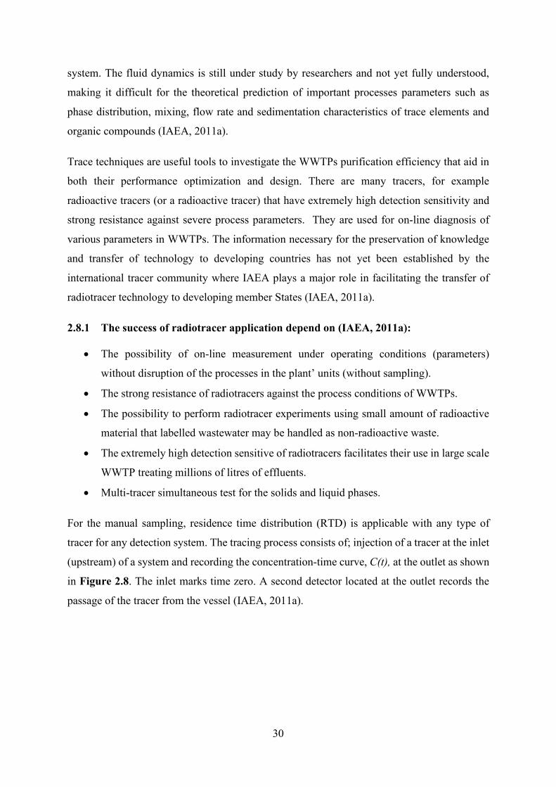
30

system. The fluid dynamics is still under study by researchers and not yet fully understood,

making it difficult for the theoretical prediction of important processes parameters such as

phase distribution, mixing, flow rate and sedimentation characteristics of trace elements and

organic compounds (IAEA, 2011a).

Trace techniques are useful tools to investigate the WWTPs purification efficiency that aid in

both their performance optimization and design. There are many tracers, for example

radioactive tracers (or a radioactive tracer) that have extremely high detection sensitivity and

strong resistance against severe process parameters. They are used for on-line diagnosis of

various parameters in WWTPs. The information necessary for the preservation of knowledge

and transfer of technology to developing countries has not yet been established by the

international tracer community where IAEA plays a major role in facilitating the transfer of

radiotracer technology to developing member States (IAEA, 2011a).

2.8.1 The success of radiotracer application depend on (IAEA, 2011a):

• The possibility of on-line measurement under operating conditions (parameters)

without disruption of the processes in the plant’ units (without sampling).

• The strong resistance of radiotracers against the process conditions of WWTPs.

• The possibility to perform radiotracer experiments using small amount of radioactive

material that labelled wastewater may be handled as non-radioactive waste.

• The extremely high detection sensitive of radiotracers facilitates their use in large scale

WWTP treating millions of litres of effluents.

• Multi-tracer simultaneous test for the solids and liquid phases.

For the manual sampling, residence time distribution (RTD) is applicable with any type of

tracer for any detection system. The tracing process consists of; injection of a tracer at the inlet

(upstream) of a system and recording the concentration-time curve, C(t), at the outlet as shown

in Figure 2.8. The inlet marks time zero. A second detector located at the outlet records the

passage of the tracer from the vessel (IAEA, 2011a).

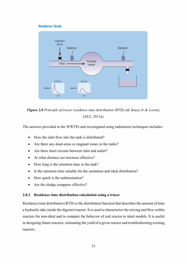
31

Figure 2.8 Principle of tracer residence time distribution (RTD) (de Souza Jr & Lorenz;

IAEA, 2011a).

The answers provided in the WWTPs and investigated using radiotracer techniques includes:

• How the inlet flow into the tank is distributed?

• Are there any dead areas or stagnant zones in the tanks?

• Are there short circuits between inlet and outlet?

• At what distance are mixtures effective?

• How long is the retention time in the tank?

• Is the retention time suitable for the sanitation and ideal distribution?

• How quick is the sedimentation?

• Are the sludge scrappers effective?

2.8.2 Residence time distribution calculation using a tracer

Residence time distribution (RTD) is the distribution function that describes the amount of time

a hydraulic take inside the digester/reactor. It is used to characterize the mixing and flow within

reactors for non-ideal and to compare the behavior of real reactor to ideal models. It is useful

in designing future reactors, estimating the yield of a given reactor and troubleshooting existing

reactors.

32

The non-ideality of industrial processes leads researchers to develop corrections to the ideal

models with less restriction. RTD is a function that describes the evolution of the average

instantaneous concentration against the elapsed time and expressed as normalized (Stenstrom,

2003).

At the tracer injection the concentration C0 is always low at the beginning, however it increases

with time due to flux in the reactor. If Co is the concentration of the tracer at the inlet of the

reactor, The fraction of tracer remaining in the reactor (F) of the tracer at the outlet of the

reactor will be given by the following Equations 2.1-2.4 (de Souza Jr & Lorenz):

𝐹𝐹(𝑡𝑡) = (𝐶𝐶(𝑡𝑡)𝐶𝐶0

………………………………….……………..………Eq. 2.1

The tracer concentration in the reactor outlet is given by:

𝐶𝐶(𝑡𝑡) = 𝐶𝐶0 ∫ 𝐸𝐸(𝑡𝑡)𝑡𝑡0 𝑑𝑑𝑡𝑡……………………………………………………….Eq. 2.2

Combining equation 2.1 and 2.2 gives

𝐹𝐹(𝑡𝑡) = ∫ 𝐸𝐸(𝑡𝑡)𝑑𝑑𝑡𝑡𝑡𝑡0 ………………………………………………………….Eq. 2.3

𝐸𝐸 (𝑡𝑡) = 𝑑𝑑𝑑𝑑(𝑡𝑡)𝑑𝑑𝑡𝑡

…………………………………….…………………………Eq. 2.4

The residence time distribution curve is shown in Figure 2.9. The curves can be analyzed

quantitatively and the behaviour of the flow inside the reactor can be outlined and observed.

Figure 2.9: Residence time distribution curve behavior

33

The E curve is the distribution needed to account for non-ideal flow (Stenstrom, 2003).

Residence time (τ) is another important parameter that needs to be determined. It is the time

that certain number of molecules has remained within a unit volume. For a fixed volume (V)

and flow rate (Q), the mean residence time ideal is given by Equation 2.5 (de Souza Jr &

Lorenz):

τ = 𝑉𝑉𝑄𝑄

………………………………………………………………………….. Eq. 2.5

Residence time distribution in the biochemical processes is related to hydraulic residence time

and bacteria residence time.

2.9 Economic Benefits of the Tracer Utilization in Wastewater Treatment Plant

Tracer technology allows movement of organic compounds and trace elements to be measured

in a range of wastewater application technologies. The tracer benefits includes (IAEA, 2011a):

• Cost effective monitoring technique

• Insight into many areas of water quality

• Sludge behaviour

• Plant processes:

WWTP flow balancing

Determination of effective volume in anaerobic digesters

Retention efficiency of storm tanks

Sediments dynamic studies

Location and quantification of sewage network infiltration.

• Enable clients to identify areas where substantial savings in both capital and operational

expenditure can be made.

• It reduces environmental impact of waste discharge.

• Provides data for the design of future plants

• Validation or/and provision of empirical data for computer fluid dynamics (CFD)

models

The experiment design consist in selection of tracer injection points, position of detectors,

radioisotopes transportation, radiological safety consideration, tracer injection, data

acquisition, treatment and interpretation (Rivera et al., 2012).

34

2.10 Conventional Tracer for WWTPs

The major non-radioactive tracers used for investigation of WWTPs units are optical and

chemical tracers.

2.10.1 Chemical tracer

Chemical tracer is easily detectable substance measurable off-line (by sampling) at very low

concentration by instrumental analytical techniques such as, gas chromatography (GC), high

performance liquid chromatography, neuron activation analysis, inductive coupled plasma

spectroscopy (ICP), etc. (IAEA, 2011a).

Sodium dichromate, sodium chloride, sodium iodide, sodium nitrite, potassium chloride,

manganese sulphate, sodium pertechnetate and lithium chloride are actively used for water

tracing in hydrology although they are not suitable and convenient to be used in WWTPs units

according to IAEA (IAEA, 2011a; Rivera et al., 2012). However, lithium chloride solution as

tracer was reported to be of use in WWTPs as reported by IAEA (IAEA, 2011a).

The advantages of lithium chloride include:

• It has no toxicity

• It does not react or degrade in wastewater

• It has a low detection and measurement limits (atomic absorption spectrometry)

2.10.2 Optical tracers

Optical tracer is divided into two categories (IAEA, 2011a):

• Colour tracer

• Fluorescent tracer

In colour tracers, the detected parameter is the colour of tracer which is measured through a

light or laser beam where a wavelength has to be adapted to fluid in order not to be absorbed

in it.

The fluorescent tracer is excited by a laser beam or light that mainly operates in the ultraviolet

(UV) region. The fluorescent tracer using Rhodamine WT and a fluorometer are reported for

online investigation of water phase dynamics in some WWTP units (designs, Accessed 2016;

IAEA, 2011a).

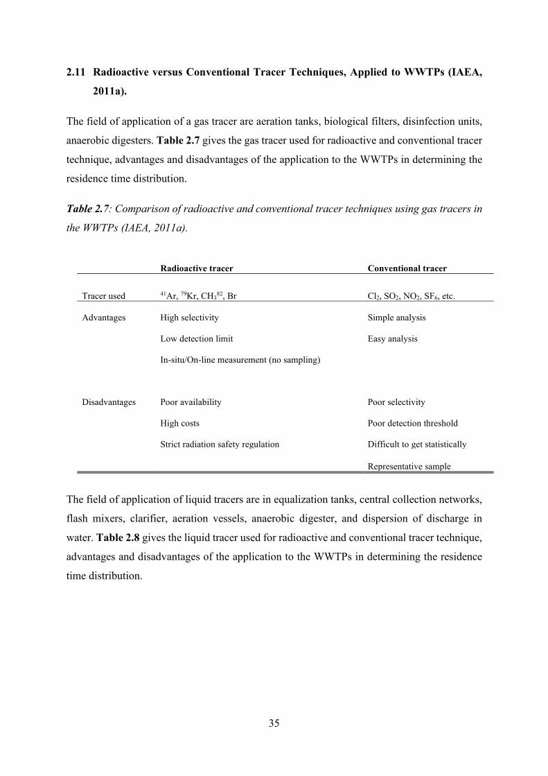
35

2.11 Radioactive versus Conventional Tracer Techniques, Applied to WWTPs (IAEA,

2011a).

The field of application of a gas tracer are aeration tanks, biological filters, disinfection units,

anaerobic digesters. Table 2.7 gives the gas tracer used for radioactive and conventional tracer

technique, advantages and disadvantages of the application to the WWTPs in determining the

residence time distribution.

Table 2.7: Comparison of radioactive and conventional tracer techniques using gas tracers in

the WWTPs (IAEA, 2011a).

Radioactive tracer Conventional tracer

Tracer used 41Ar, 79Kr, CH382, Br Cl2, SO2, NO2, SF6, etc.

Advantages High selectivity Simple analysis

Low detection limit Easy analysis

In-situ/On-line measurement (no sampling)

Disadvantages Poor availability Poor selectivity

High costs Poor detection threshold

Strict radiation safety regulation Difficult to get statistically

Representative sample

The field of application of liquid tracers are in equalization tanks, central collection networks,

flash mixers, clarifier, aeration vessels, anaerobic digester, and dispersion of discharge in

water. Table 2.8 gives the liquid tracer used for radioactive and conventional tracer technique,

advantages and disadvantages of the application to the WWTPs in determining the residence

time distribution.

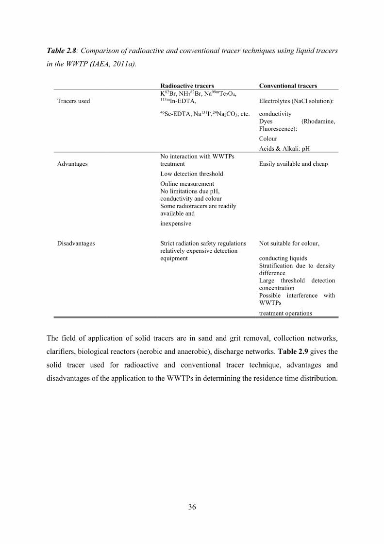
36

Table 2.8: Comparison of radioactive and conventional tracer techniques using liquid tracers

in the WWTP (IAEA, 2011a).

Radioactive tracers Conventional tracers

Tracers used K82Br, NH3

82Br, Na99mTc2O4, 113mIn-EDTA, Electrolytes (NaCl solution):

46Sc-EDTA, Na131I-,24Na2CO3, etc. conductivity

Dyes (Rhodamine, Fluorescence):

Colour Acids & Alkali: pH

Advantages No interaction with WWTPs

treatment Easily available and cheap Low detection threshold Online measurement

No limitations due pH,

conductivity and colour

Some radiotracers are readily

available and inexpensive Disadvantages Strict radiation safety regulations Not suitable for colour,

relatively expensive detection

equipment conducting liquids

Stratification due to density difference

Large threshold detection concentration

Possible interference with WWTPs

treatment operations

The field of application of solid tracers are in sand and grit removal, collection networks,

clarifiers, biological reactors (aerobic and anaerobic), discharge networks. Table 2.9 gives the

solid tracer used for radioactive and conventional tracer technique, advantages and

disadvantages of the application to the WWTPs in determining the residence time distribution.

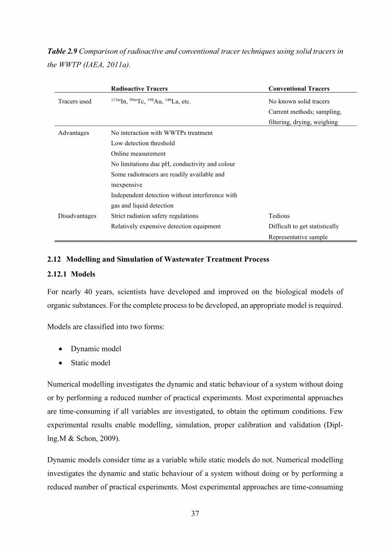
37

Table 2.9 Comparison of radioactive and conventional tracer techniques using solid tracers in

the WWTP (IAEA, 2011a).

Radioactive Tracers Conventional Tracers

Tracers used 113mIn, 99mTc, 198Au, 140La, etc. No known solid tracers Current methods; sampling, filtering, drying, weighing Advantages No interaction with WWTPs treatment Low detection threshold Online measurement No limitations due pH, conductivity and colour Some radiotracers are readily available and inexpensive Independent detection without interference with gas and liquid detection Disadvantages Strict radiation safety regulations Tedious Relatively expensive detection equipment Difficult to get statistically

Representative sample

2.12 Modelling and Simulation of Wastewater Treatment Process

2.12.1 Models

For nearly 40 years, scientists have developed and improved on the biological models of

organic substances. For the complete process to be developed, an appropriate model is required.

Models are classified into two forms:

• Dynamic model

• Static model

Numerical modelling investigates the dynamic and static behaviour of a system without doing

or by performing a reduced number of practical experiments. Most experimental approaches

are time-consuming if all variables are investigated, to obtain the optimum conditions. Few

experimental results enable modelling, simulation, proper calibration and validation (Dipl-

lng.M & Schon, 2009).

Dynamic models consider time as a variable while static models do not. Numerical modelling

investigates the dynamic and static behaviour of a system without doing or by performing a

reduced number of practical experiments. Most experimental approaches are time-consuming

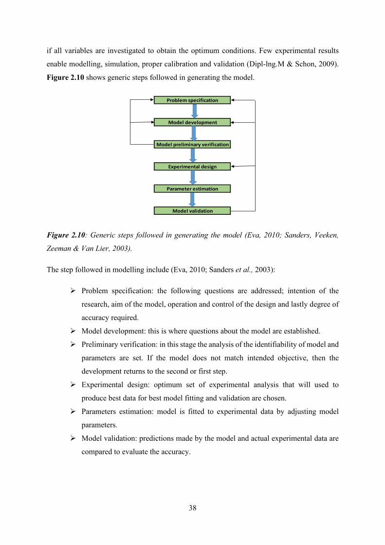
38

if all variables are investigated to obtain the optimum conditions. Few experimental results

enable modelling, simulation, proper calibration and validation (Dipl-lng.M & Schon, 2009).

Figure 2.10 shows generic steps followed in generating the model.

Figure 2.10: Generic steps followed in generating the model (Eva, 2010; Sanders, Veeken,

Zeeman & Van Lier, 2003).

The step followed in modelling include (Eva, 2010; Sanders et al., 2003):

Problem specification: the following questions are addressed; intention of the

research, aim of the model, operation and control of the design and lastly degree of

accuracy required.

Model development: this is where questions about the model are established.

Preliminary verification: in this stage the analysis of the identifiability of model and

parameters are set. If the model does not match intended objective, then the

development returns to the second or first step.

Experimental design: optimum set of experimental analysis that will used to

produce best data for best model fitting and validation are chosen.

Parameters estimation: model is fitted to experimental data by adjusting model

parameters.

Model validation: predictions made by the model and actual experimental data are

compared to evaluate the accuracy.

Problem specification

Model development

Model preliminary verification

Experimental design

Parameter estimation

Model validation

39

2.12.2 Advantage of modelling in wastewater treatment processes

The most prominent advantages of using the models in wastewater treatment process, are

(Henze, 2008):

Evaluating possible scenarios for upgrading

Evaluating new plant design

Supporting management decisions

Developing new control schemes

Providing operator training

Saving time and money in the process of technology/process selection.

Comparison of the system performance in a quantitative instead of a qualitative way

allows in many cases for easier decision‐making and rapid comparison of options

(Henze, 2008).

The second main reason for using model is the possibility of saving time and money in the

process of technology/process selection. Comparison of the system performance in a

quantitative instead of a qualitative way allows in many cases, for easier decision‐making and

rapid comparison of options (Henze, 2008).

Another strong reason for using model is the possibility of minimizing risks. By using model,

‘what if’ scenarios can be examined in a quantitative way in respect of what the effects of

potential risks are. Furthermore, application of models improves knowledge transfer and

decision‐making (Henze, 2008).

2.12.3 Mass balance analysis

Mass balance is the fundamental approach used to study the hydraulic flow characteristic of

reactors/digesters and to delineate the changes that takes place when a reaction takes place. It

defines what occurs in the treatment reactors as a function of hydraulic retention time. It is

based on the principle of mass conservation or law of conservation of mass, where mass is

neither created or destroyed but may transformed from one form to another (e.g. solid to liquid

to gases) (E. Metcalf). Mass balance for the heavy metals in primary, secondary and the whole

WWTPs process shows good closures for all metals species (Karvelas, Katsoyiannis & Samara,

2003).

40

The general steps used in preparing the mass balance analyses includes (E. Metcalf) :

Preparing a flow diagram or a simplified schematic of the system or the process for

which mass balance is to be prepared.

Drawing a system or control volume boundary to define the limits over which the

mass balance is to be applied.

List all of the assumptions and pertinent data that will be used in the preparation of

the material balance on the schematics of flow diagram.

Select a convenient basis on which the numerical calculation will be used.

To apply a mass-balance analysis to the liquid contents of the reactor in WWTPs, it will be

assumed that (E. Metcalf):

The volumetric flowrates into and out of the container is constant.

The liquid within the reactor is not subject to evaporation (isothermal conditions)

The liquid within the container is mixed completely

A chemical reaction involving the reactant C is occurring within the reactor

The rate of change in the concentration of the reactant C occurring within the reactor

is governed by a first-order reaction (rc= -kC-decrease in the reactant while rc=

+kC-increase in the reactant).

The general mass balance equation is given by.

Rate of

accumulation =

Rate of flow

the - Rate of flow +

Rate of generation

(utilization)

of reactant within

of reactant into

of reactant out of

of reactant within

the system

boundary

system

boundary

the system

boundary

the system boundary

The corresponding simplified word statement is given by Equation 2.6:

Accumulation = Inflow – Outflow + Generation Eq. 2.6

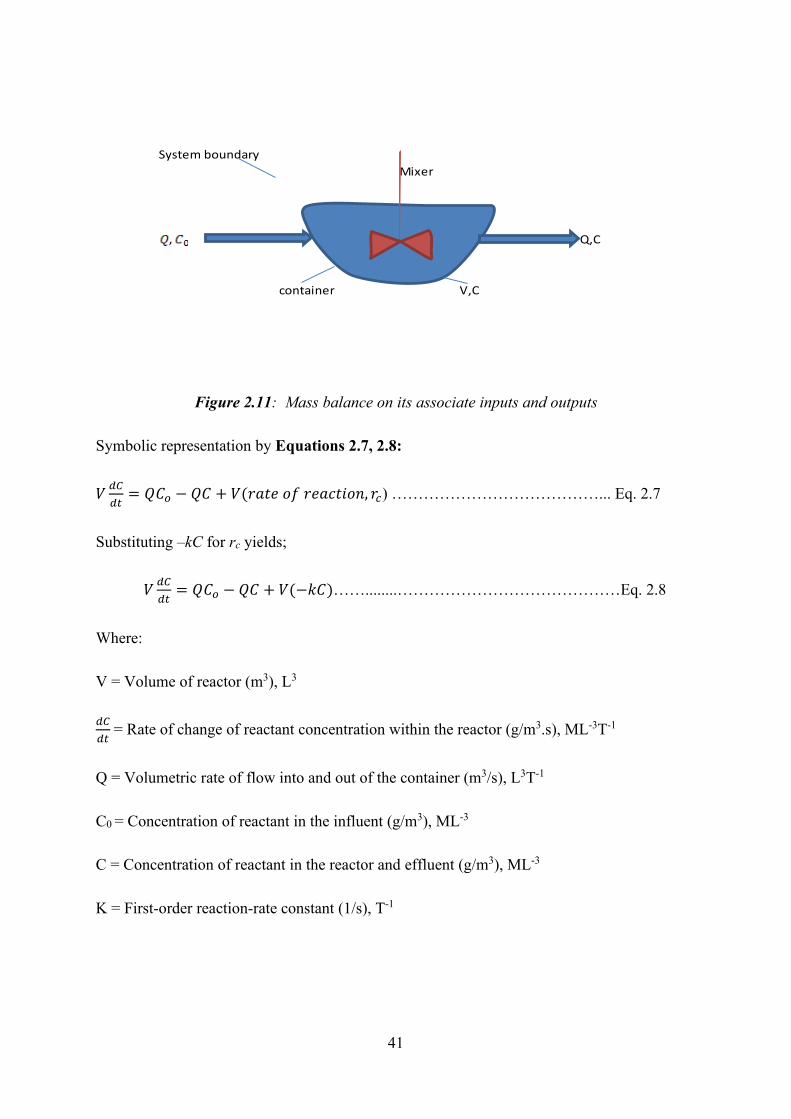
41

Figure 2.11: Mass balance on its associate inputs and outputs

Symbolic representation by Equations 2.7, 2.8:

𝑉𝑉 𝑑𝑑𝐶𝐶𝑑𝑑𝑡𝑡

= 𝑄𝑄𝐶𝐶𝑜𝑜 − 𝑄𝑄𝐶𝐶 + 𝑉𝑉(𝑟𝑟𝑟𝑟𝑡𝑡𝑟𝑟 𝑜𝑜𝑜𝑜 𝑟𝑟𝑟𝑟𝑟𝑟𝑟𝑟𝑡𝑡𝑟𝑟𝑜𝑜𝑟𝑟, 𝑟𝑟𝑐𝑐) …………………………………... Eq. 2.7

Substituting –kC for rc yields;

𝑉𝑉 𝑑𝑑𝐶𝐶𝑑𝑑𝑡𝑡

= 𝑄𝑄𝐶𝐶𝑜𝑜 − 𝑄𝑄𝐶𝐶 + 𝑉𝑉(−𝑘𝑘𝐶𝐶)……........……………………………………Eq. 2.8

Where:

V = Volume of reactor (m3), L3

𝑑𝑑𝐶𝐶𝑑𝑑𝑡𝑡

= Rate of change of reactant concentration within the reactor (g/m3.s), ML-3T-1

Q = Volumetric rate of flow into and out of the container (m3/s), L3T-1

C0 = Concentration of reactant in the influent (g/m3), ML-3

C = Concentration of reactant in the reactor and effluent (g/m3), ML-3

K = First-order reaction-rate constant (1/s), T-1

System boundaryMixer

Q,C

container V,C

42

2.12.4 Different types of models

Several mathematical models are available to describe the biochemical transformation and

degradation processes in WWTPs. The most popular is the IWA (International Water

Association) Activated Sludge Model (ASM) and Anaerobic Digestion Model 1 (ADM1)

family (Henze et al., 2000). ASM1 and ADM1 are very extensively used in the wastewater

community and has become the standard model for dynamic simulation of activated sludge

plants (Langergraber et al., 2004a).

Other types of the model for WWTPs include:

• DTS Pro-Modelling of gas, liquid and solid flows at a steady theoretical interpretation

framework for tracer.

• ASM2/2d are able to describe enhanced biological and chemical removal

(Langergraber et al., 2004a).

• ASM3 introduced a new set of processes to describe the COD flow (Langergraber et

al., 2004a).

• ASAL models for BOD removal (Langergraber et al., 2004a).

• Lawrence and McCarty model for COD and nutrients removal (H.).

• ADM1 as proposed by the International Water Association (IWA) group deals with

mathematical modelling of anaerobic digestion processes by Batstone et al., 2002a

(Eelke, 2014).

• Biosorption equilibrium models for metal removal.

2.12.5 Bio-chemical kinetics models

The theory of biological processes has been previously represented mathematically to represent

process kinetics (Porubova et al., 2011). Most of the models allow biological treatment process

calculations. This allows monitoring parameters and enhancing plant efficiency. The following

are some common kinetic expressions describing biological treatment (Gerber & Span, 2008):

Biosorption equilibrium models

First order kinetic model

Monod kinetic model

Chen and Hashimoto kinetic model

Contois kinetic model

43

Modified Gompertz kinetic model

Michaelis-Menten kinetic model

Anaerobic Digestion Model (ADM1)

Activated Sludge Models (ASM)

Biosorption equilibrium models

2.12.6 Identification of constraints for the modelling scenarios:

The constraints include equipment constraints such as lower capacities, pump limits, potential

unit out of service. And the operating constraint that includes solids retention time for

nitrification, anaerobic digester HRT, maximum allowable mixed liquor concentration,

dewatering facility operating shift length.

2.12.6.1 Establish key performance indicators (KPIs)

This involves which parameters should be tracked and it serves as a model output.

2.12.6.2 Establish modelling scenarios

This identifies temperature, flow and load pattern to apply in conjunction with estimated future

daily average flows and whether a plant can accommodate an additional input from a nearby

plant.

2.12.6.3 Run modelling scenarios

It is important to run model iteratively, particularly if the objective is to determine the ultimate

plant capacity with existing infrastructure.

2.13 Standards of Organics and Inorganics in Wastewater

Table 2.13 shows the water standards enacted by-law in various Government and Non-

Government institution Worldwide. It summarizes different substances/parameters

concentration. The American National Safe Drinking Water Act (SDWA) signed in 1974 and

enacted by the Environmental Protection Agency (EPA) shows the contaminants; organics,

inorganics, radionuclides and microbial, maximum contaminants level (MCLs) for the public

water quality standards, best available technology (BAT) and potential health effects.

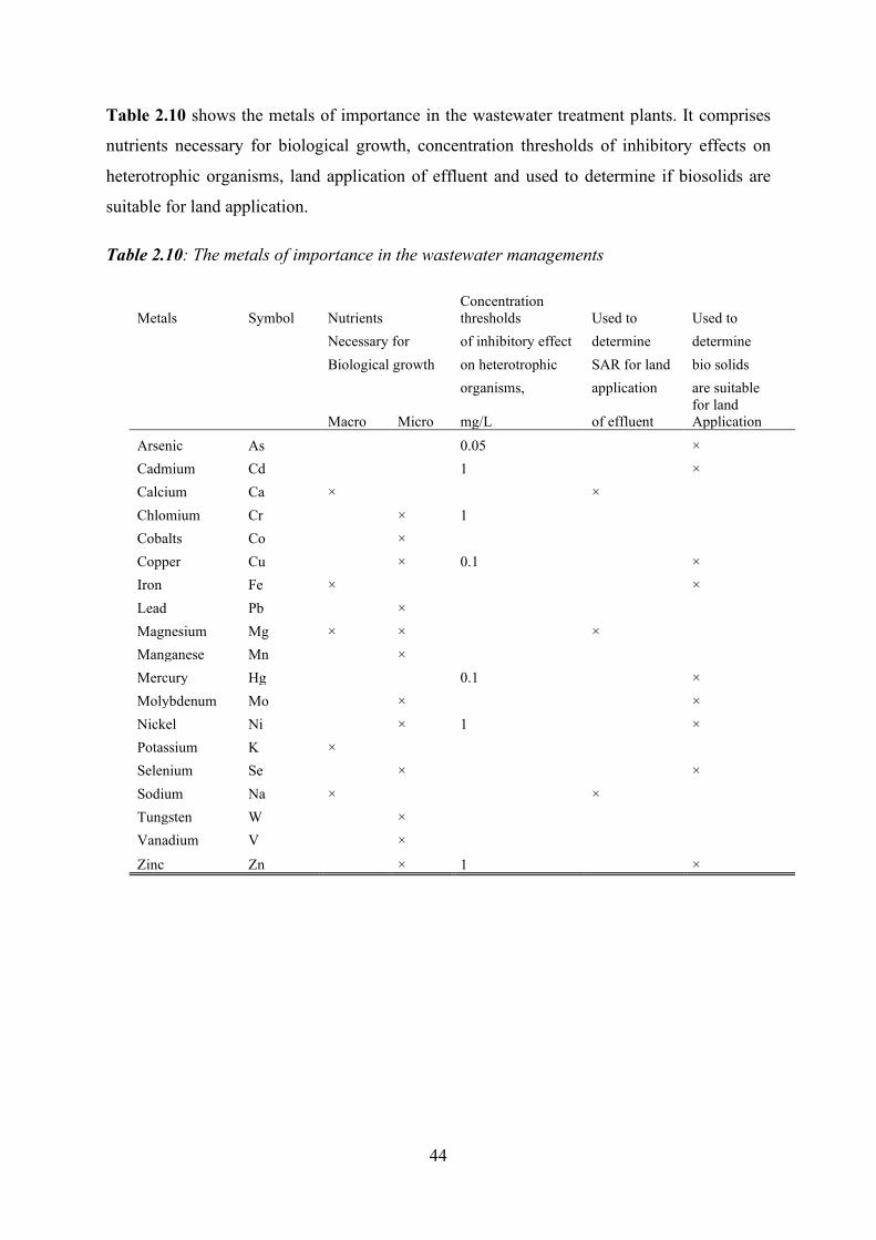
44

Table 2.10 shows the metals of importance in the wastewater treatment plants. It comprises

nutrients necessary for biological growth, concentration thresholds of inhibitory effects on

heterotrophic organisms, land application of effluent and used to determine if biosolids are

suitable for land application.

Table 2.10: The metals of importance in the wastewater managements

Metals Symbol Nutrients Concentration thresholds Used to Used to

Necessary for of inhibitory effect determine determine Biological growth on heterotrophic SAR for land bio solids organisms, application are suitable

Macro Micro mg/L of effluent for land Application

Arsenic As 0.05 × Cadmium Cd 1 × Calcium Ca × × Chlomium Cr × 1 Cobalts Co × Copper Cu × 0.1 × Iron Fe × × Lead Pb × Magnesium Mg × × × Manganese Mn × Mercury Hg 0.1 × Molybdenum Mo × × Nickel Ni × 1 × Potassium K × Selenium Se × × Sodium Na × × Tungsten W × Vanadium V ×

Zinc Zn × 1 ×

45

2.14 Sources of Trace Metals in Wastewater Treatment Plant

Trace elements pollution has attracted much attention in recent years due to its

bioaccumulation, toxicity and wide range of sources and persistence (Wang et al., 2015).

Besides the toxicity caused by inorganic metals, the latter also affect the ecosystems of the

receiving water (Berkun & Onal, 2004). The presence of these metals (e.g. Pb, Cd, Cr, Cu, Zn,

As, Mn, Al, etc.) are brought about by industrial activities that generate numerous chemical

elements (Wang et al., 2015). The metals concentrations could be analyzed by the use of

inductively coupled plasma-optical emission spectroscopy (ICP-OES), inductively coupled

plasma-mass spectrometry (ICP-MS), flame atomic absorption spectrometry (FAAS), and

graphite furnace atomic absorption spectrometry (GFAAS) (Mogolodi, Ngila & Mabuba, 2015;

Shamuyarira & Gumbo, 2014). Several methods have been developed for the removal of heavy

metal in the wastewater such as evaporation, precipitation, electroplating, membrane processes,

ion exchange, etc. These methods have several demerits such as high reagent requirement,

unpredictable metal ion removal, etc. (Das, Vimala & Karthika, 2008).

Metals are involved in metabolism and microbial growth in WWTPs. Essential metals like Ca,

Cu, Co, Fe, K, Mg, Mn and those with non-essential biological functions such as Al, Cd, Cs,

Hg, Pb, and Hg can be accumulated by microorganisms through non-specific physio-chemical

interactions as well as specific mechanisms of sequential transport (Barakat, 2011; Karvelas

et al., 2003; Van Wyk, 2011). Thus, research studies should be undertaken in order to construct

historical records of contamination and quantification of the intensity of heavy metal pollution

based on enrichment factor, risk assessment codes (RAC) and excess flux. Investigation of the

sources of heavy metals by assessing speciation relationships through component analysis, is

crucial (Wang et al., 2015).

2.15 Levels of Metals in WWTPs in Gauteng

In seven of the nine provinces of South Africa, more than half the water is provided by inter-

basin transfers (DWS, 2016). This demonstrates the intensity with which the country’s

available resources are already being used. The current status of water quality varies

substantially, with the most contaminated water resources being the Vaal River, Crocodile

West (Limpopo), Umgeni and Olifants River systems. Radionuclide and heavy metal

contamination in South Africa are the legacy of more than a century of unregulated gold

mining, coupled with high-density populations living in daily close contact with dust and

sediment arising from mine tailings dams (Van der Merwe-Botha, 2009). Parts of Soweto and

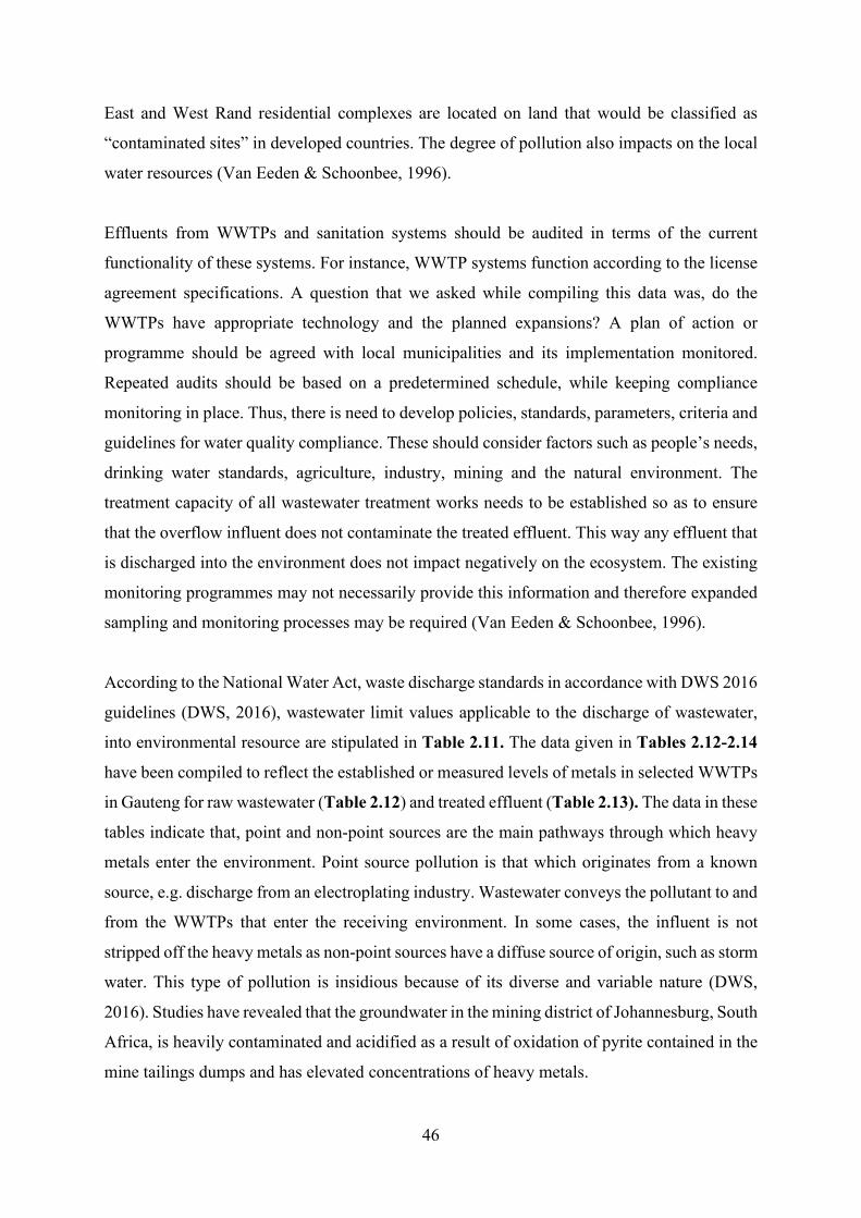
46

East and West Rand residential complexes are located on land that would be classified as

“contaminated sites” in developed countries. The degree of pollution also impacts on the local

water resources (Van Eeden & Schoonbee, 1996).

Effluents from WWTPs and sanitation systems should be audited in terms of the current

functionality of these systems. For instance, WWTP systems function according to the license

agreement specifications. A question that we asked while compiling this data was, do the

WWTPs have appropriate technology and the planned expansions? A plan of action or

programme should be agreed with local municipalities and its implementation monitored.

Repeated audits should be based on a predetermined schedule, while keeping compliance

monitoring in place. Thus, there is need to develop policies, standards, parameters, criteria and

guidelines for water quality compliance. These should consider factors such as people’s needs,

drinking water standards, agriculture, industry, mining and the natural environment. The

treatment capacity of all wastewater treatment works needs to be established so as to ensure

that the overflow influent does not contaminate the treated effluent. This way any effluent that

is discharged into the environment does not impact negatively on the ecosystem. The existing

monitoring programmes may not necessarily provide this information and therefore expanded

sampling and monitoring processes may be required (Van Eeden & Schoonbee, 1996).

According to the National Water Act, waste discharge standards in accordance with DWS 2016

guidelines (DWS, 2016), wastewater limit values applicable to the discharge of wastewater,

into environmental resource are stipulated in Table 2.11. The data given in Tables 2.12-2.14

have been compiled to reflect the established or measured levels of metals in selected WWTPs

in Gauteng for raw wastewater (Table 2.12) and treated effluent (Table 2.13). The data in these

tables indicate that, point and non-point sources are the main pathways through which heavy

metals enter the environment. Point source pollution is that which originates from a known

source, e.g. discharge from an electroplating industry. Wastewater conveys the pollutant to and

from the WWTPs that enter the receiving environment. In some cases, the influent is not

stripped off the heavy metals as non-point sources have a diffuse source of origin, such as storm

water. This type of pollution is insidious because of its diverse and variable nature (DWS,

2016). Studies have revealed that the groundwater in the mining district of Johannesburg, South

Africa, is heavily contaminated and acidified as a result of oxidation of pyrite contained in the

mine tailings dumps and has elevated concentrations of heavy metals.

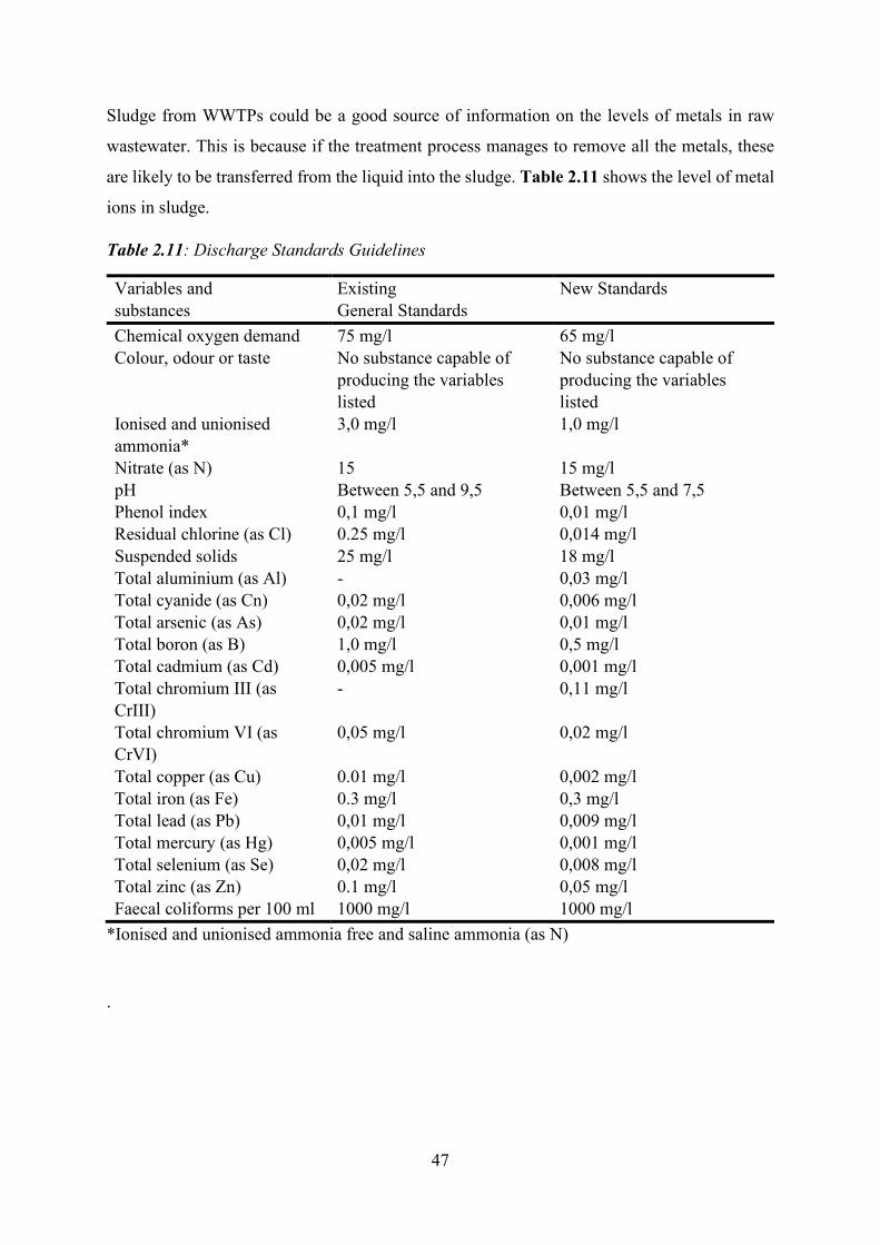
47

Sludge from WWTPs could be a good source of information on the levels of metals in raw

wastewater. This is because if the treatment process manages to remove all the metals, these

are likely to be transferred from the liquid into the sludge. Table 2.11 shows the level of metal

ions in sludge.

Table 2.11: Discharge Standards Guidelines

Variables and substances

Existing General Standards

New Standards

Chemical oxygen demand 75 mg/l 65 mg/l Colour, odour or taste No substance capable of

producing the variables listed

No substance capable of producing the variables listed

Ionised and unionised ammonia*

3,0 mg/l 1,0 mg/l

Nitrate (as N) 15 15 mg/l pH Between 5,5 and 9,5 Between 5,5 and 7,5 Phenol index 0,1 mg/l 0,01 mg/l Residual chlorine (as Cl) 0.25 mg/l 0,014 mg/l Suspended solids 25 mg/l 18 mg/l Total aluminium (as Al) - 0,03 mg/l Total cyanide (as Cn) 0,02 mg/l 0,006 mg/l Total arsenic (as As) 0,02 mg/l 0,01 mg/l Total boron (as B) 1,0 mg/l 0,5 mg/l Total cadmium (as Cd) 0,005 mg/l 0,001 mg/l Total chromium III (as CrIII)

- 0,11 mg/l

Total chromium VI (as CrVI)

0,05 mg/l 0,02 mg/l

Total copper (as Cu) 0.01 mg/l 0,002 mg/l Total iron (as Fe) 0.3 mg/l 0,3 mg/l Total lead (as Pb) 0,01 mg/l 0,009 mg/l Total mercury (as Hg) 0,005 mg/l 0,001 mg/l Total selenium (as Se) 0,02 mg/l 0,008 mg/l Total zinc (as Zn) 0.1 mg/l 0,05 mg/l Faecal coliforms per 100 ml 1000 mg/l 1000 mg/l

*Ionised and unionised ammonia free and saline ammonia (as N)

.

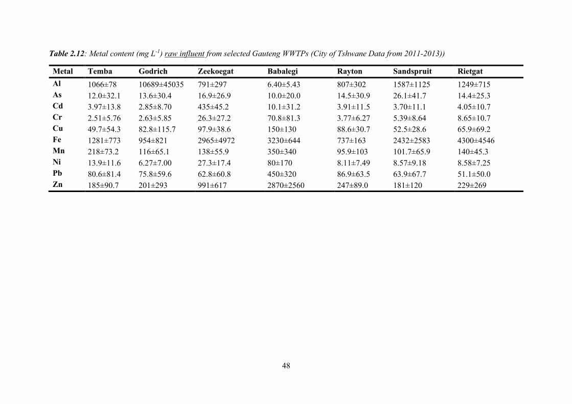
48

Table 2.12: Metal content (mg L-1) raw influent from selected Gauteng WWTPs (City of Tshwane Data from 2011-2013))

Metal Temba Godrich Zeekoegat Babalegi Rayton Sandspruit Rietgat Al 1066±78 10689±45035 791±297 6.40±5.43 807±302 1587±1125 1249±715 As 12.0±32.1 13.6±30.4 16.9±26.9 10.0±20.0 14.5±30.9 26.1±41.7 14.4±25.3 Cd 3.97±13.8 2.85±8.70 435±45.2 10.1±31.2 3.91±11.5 3.70±11.1 4.05±10.7 Cr 2.51±5.76 2.63±5.85 26.3±27.2 70.8±81.3 3.77±6.27 5.39±8.64 8.65±10.7 Cu 49.7±54.3 82.8±115.7 97.9±38.6 150±130 88.6±30.7 52.5±28.6 65.9±69.2 Fe 1281±773 954±821 2965±4972 3230±644 737±163 2432±2583 4300±4546 Mn 218±73.2 116±65.1 138±55.9 350±340 95.9±103 101.7±65.9 140±45.3 Ni 13.9±11.6 6.27±7.00 27.3±17.4 80±170 8.11±7.49 8.57±9.18 8.58±7.25 Pb 80.6±81.4 75.8±59.6 62.8±60.8 450±320 86.9±63.5 63.9±67.7 51.1±50.0 Zn 185±90.7 201±293 991±617 2870±2560 247±89.0 181±120 229±269

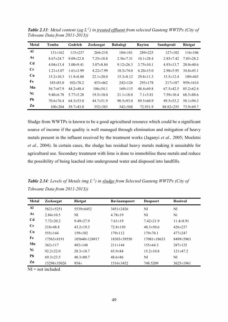
49

Table 2.13: Metal content (µg L-1) in treated effluent from selected Gauteng WWTPs (City of Tshwane Data from 2011-2013))

Metal Temba Godrich Zeekoegat Babalegi Rayton Sandspruit Rietgat

Al 131±162 115±237 264±218 184±181 289±225 127±102 116±106 As 8.67±24.7 9.09±22.8 7.25±18.8 2.56±7.31 10.1±28.4 2.85±7.42 7.85±28.2 Cd 4.04±13.4 3.00±9.41 3.07±8.84 9.12±26.3 3.75±10.1 4.93±13.7 20.0±40.6 Cr 1.21±3.07 1.61±3.99 4.22±7.99 18.5±74.0 6.20±15.0 2.98±5.95 34.8±45.1 Cu 15.2±10.3 11.9±8.88 22.1±20.0 15.3±8.12 29.8±11.3 15.5±12.4 109±443 Fe 185±83.0 102±70.2 453±462 242±126 293±178 217±187 959±1614 Mn 56.7±67.9 44.2±48.4 106±54.1 169±115 48.4±69.8 67.5±42.5 85.2±62.4 Ni 9.40±6.78 5.77±5.28 19.5±10.0 21.1±18.0 7.1±5.81 7.59±10.4 68.5±88.6 Pb 70.6±76.4 64.3±53.0 44.7±51.9 90.5±93.0 89.5±60.9 49.5±53.2 58.1±94.3 Zn 100±204 39.7±43.0 352±383 342±568 72.931.9 88.82±255 73.9±69.7

Sludge from WWTPs is known to be a good agricultural resource which could be a significant

source of income if the quality is well managed through elimination and mitigation of heavy

metals present in the influent received by the treatment works (Jaganyi et al., 2005; Moeletsi

et al., 2004). In certain cases, the sludge has residual heavy metals making it unsuitable for

agricultural use. Secondary treatment with lime is done to immobilise these metals and reduce

the possibility of being leached into underground water and disposed into landfills.

Table 2.14: Levels of Metals (mg L-1) in sludge from Selected Gauteng WWTPs (City of

Tshwane Data from 2011-2013))

Metal Zeekoegat Rietgat Baviaanspoort Daspoort Rooiwal

Al 5621±5251 5539±6452 3451±2426 NI NI As 2.84±10.5 NI 4.78±19 NI Ni Cd 7.72±20.2 9.49±27.9 7.61±19 7.42±21.9 11.4±8.91 Cr 218±48.8 43.2±19.3 72.8±150 48.3±50.6 426±237 Cu 555±144 159±102 179±112 179±70.1 477±247 Fe 17563±8191 105640±124917 18303±39550 17081±18633 8499±5963 Mn 362±117 492±148 211±144 155±64.3 287±125 Ni 92.2±22.0 28.3±18.7 65.9±84 15.2±10.8 121±47.2 Pb 69.3±23.5 48.3±80.7 48.6±86 NI NI Zn 15298±35026 954± 1516±3452 748.5209 3625±1961

NI = not included

50

2.16 Organic Compounds in Water and Sludge in WWTPs, Gauteng Province

Most of the organic contaminants in wastewater originates from products that are used in

everyday life and in very large quantities such as pharmaceuticals, personal care products,

pesticides, PAHs among others. Numerous previous studies have indicated that these

compounds undergo partial or no removal during treatment processes and are therefore

detected in the effluent water and in aquatic environments. These emerging compounds were

also not included in the relevant legislation for monitoring and hence there were no limit values

set for treated wastewater (Thomaidi, Stasinakis, Borova & Thomaidis, 2015).

Within the water treatment plants, there is secondary contamination which occurs from the

different processes within the plant used in treating the water. A well-known example is the

disinfection by-products (DBPS) which occur as a result of disinfection with, chlorine,

chloramine, ozone, chlorine dioxide with natural organic matter (NOM) and iodide or bromide

(Richardson & Ternes, 2011). These by-products include trihalomethanes (THMs) and

haloacetic acids, both of which are suspected human carcinogens and are now regulated by the

EPA for DBPs with the maximum contaminant levels of 80 and 60 µg/L, respectively (Zazouli

et al., 2007). Other DBPs include nitrosamines, bromonitromethanes iodo-trihalomethanes,

haloaldehydes, and halonitromethanes (Richardson & Ternes, 2011).

Emerging pollutants are defined as compounds that are not currently covered by existing water-

quality regulations. They are usually present in surface waters at trace levels and cause known

or suspected adverse ecological and/or human health effects (Boleda, Galceran & Ventura,

2011; Farré, Pérez, Kantiani & Barceló, 2008; Geissen et al., 2015). Modern society depends

on a large range of organic chemicals and compounds which ultimately enter urban wastewater,

posing potential environmental threats to the living (Bolong, Ismail, Salim & Matsuura, 2009;

Clarke & Smith, 2011). The examples of emerging pollutants found in wastewater include

endocrine disruptors compounds (EDCs), pharmaceuticals, drugs of abuse, personal-care

products, steroids and hormones, surfactants, perfluorinated compounds, flame retardants,

industrial additives and agents, gasoline additives,1,4-dioxane and swimming pool disinfection

by-products (Farré et al., 2008).

2.16.1 Polyaromatic hydrocarbons (PAHs)

PAHs are a class of diverse organic compounds with two or more aromatic rings of carbon and

hydrogen atoms. They are reported to be among the widespread organic contaminants in

51

aquatic environments including WWTP. PAHs do not degrade easily and are persistent to the

environment with an increase in molecular weight. They bioaccumulate in food chains,

rendering them harmful and toxic to humans and living organisms, via their carcinogenic,

mutagenic, and endocrine disruption effects (Ferretto et al., 2014). Sources of PAHs include

but not limited to forest and rangeland fires, oil seeps while their anthropogenic sources are

mostly combustion of fossil fuel, coal tar, used lubricating oil, municipal incineration and

petroleum spills and discharge. They are introduced into the aquatic life via discharge of oil in

transit from oil tankers during sea activities, industrial and urban wastes as a result of surface

runoff, wastewater effluent as well as atmospheric particles (Ferretto et al., 2014; Haritash &

Kaushik, 2009). PAHs up to now have always been on the priority list of regulated

contaminants by the European union (EU) and the USEPA (Ferretto et al., 2014). Due to their

constant introduction into aquatic life, it is of high importance that they are monitored for

effective removal in the WWTP.

2.16.2 Pesticides

Pesticides comprise a collective group of organic chemical compounds used for different

purposes such fungicides, herbicides, insecticides, rodenticides among other uses. They are

mostly used in agriculture for enhanced food production worldwide. Surface run-off from

agriculturally related use has been the most predominant source of entry pesticide

contamination into the environment. However, WWTP represents one of the main sources of

contamination in urban areas mostly attributed to non-agricultural uses (Köck-Schulmeyer

et al., 2013).

Pesticides can undergo environmental degradation to from transformation products (TPs)

through various mechanisms such as biological or chemical which occur through

hydrolysis,photolysis, and/or redox reactions. TPs are on the increase as recent detailed reports

by Vidal et al., [49] indicate that they could be more persistent and toxic than the parent

compound, e.g. carbamates, organophosphorus (Zhao & Hwang, 2009) DDE which is more

persistent that DDT. The presence of natural organic matter, as well as the disinfection process

present in WWTPs, play a role in the transformation of pesticides to their metabolites. A report

by Bavcon et al. (2003) [50], investigated the formation of transformation products of two

organophosphorus, i.e malathion and diazinon under different environmental conditions

(Bavcon, Trebše & Zupančič-Kralj, 2003). There is, therefore, a need to monitor pesticides and

52

their TPs in the wastewaters as most previous methods only focused on the parent compound

(Martínez Vidal, Plaza-Bolaños, Romero-González & Garrido Frenich, 2009).

Recent work by Dabrowski et at. (2014) [52] shows a wide use of pesticides in South

Africa,with reports of atrazine, simazine and terbuthylazine being frequently reported in

ground and surface water at relatively high concentrations, in areas where there is high maize

production. Atrazine application in maize crops which is the most widely produced crop in SA,

is in the tune of 1014.42 × 103 kg. This is a huge volume of pesticides and if not well monitored

for effective removal in wastewaters will ultimately be recycled throughout body systems via

various means of exposure aforementioned (Dabrowski, Shadung & Wepener, 2014). Hence

in this study, we shall use advanced chromatographic techniques coupled with mass

spectrometers in addition to modeling, as these instruments possess high sensitivity to ng/L

levels for developing a robust method for detecting a vast number of priority pesticides

compounds in South African wastewaters.

2.16.3 Disinfection by-products

Disinfectants are chemicals used in disinfection processes, pre-oxidation and for the removal

of taste and bad odour. Disinfection can thus be described as removal, deactivation or killing

of pathogenic microorganisms. Microorganisms are destroyed or deactivated, resulting in

termination of growth and reproduction (Peter & Freese, 2009). Disinfection in normally

carried out in the final stages of water treatment processes. Disinfection by-products (DBPs)

are toxic chemical substances formed as a result of the interaction between natural organic

matter, anthropogenic contaminants, bromide or iodide with disinfection agents such as

chlorine, chloramine, chlorine dioxide and ozone that are used in water treatment plants

(Fischer, Fries, Korner, Schmalz & Zwiener, 2012; Richardson, Plewa, Wagner, Schoeny &

DeMarini, 2007).

An intensive report was done by Richardson et al. (2007) [55], categorized the different classes

of DBPs as regulated and non-regulated (Richardson et al., 2007). The regulated ones include

trihalomethanes chloroform, bromodichloromethane, chlorodibromomethane, and

bromoform), haloacetic acid (chloroacetic acid, bromoacetic acid, chloroacetic acid, dibromo

acetic acid and trichloroacetic acid) and Oxyhalides (bromate and chlorite) (Acero, Benítez,

Real & González, 2008; Bond, Huang, Graham & Templeton, 2014). THMs were the first

reported DBPs and together with haloacetic acids (HAA), they are the most prevalent of all

DBPs, most of which are regulated by the EPA (Richardson et al., 2007). The contact pathways

53

of the THMs to humans have been reported to be via inhalation, ingestion, and dermal pathways

(Chowdhury, 2012). It has also been reported that use of UV and advanced oxidation

(UV/H2O2) increases the formation of DBPs in water treatment processes (Richardson &

Ternes, 2011). In another study, it was shown that ozonation followed by post chlorination led

to the formation of the highest number of halo nitromethanes. However, when ozone is used in

water treatment, it lowers the formation of THMs and HAAs, but the only challenge is the

presence of natural bromide at elevated levels which leads to the formation of dibromo acetic

acid, a high occurrence trans-species carcinogen (Richardson et al., 2007). Ozonation followed

by post chlorination is normally done as ozone has a short residual lifetime and hence giving

more chances for bacterial regrowth if not followed with chemical disinfection (Peter & Freese,

2009).

Halo-aldehydes, according to Richardson’s report [55], are the 3rd most prevalent DBPs after

THMs and HAAs. An example is trichloroacetaldehyde (chlorate hydrate CH), the most

common in this class. Its formation depends more on the type of NOM and increases in chlorine

dosage. Other groups of DBP include halonitromethanes, iodo-acids, halo-acids, iodo-THMs,

MX compounds, haloamides, halo acetonitriles, halopyrroles, nitrosamines, and aldehydes

(Richardson et al., 2007). In light of all of the above, it is imperative to assess the occurrence

of different classes of DBPs in South African wastewaters be conducted and hence make an

informed decision on how effectively to treat our waters with minimal risk of exposure to

environmental and human health.

2.16.4 Personal care products

The number of organic chemicals that comprise personal care products (PCPs) are in

thousands. These products are used daily and in large quantities by multitudes of individuals.

They include items such as shampoo, soaps, lotions fragrances and cosmetic products, dental

care products among others (Lubliner, Redding & Ragsdale, 2010). The organic compounds of

concern present in these products include but not limited to UV filter (e.g. benzophenone),

preservative (e.g. parabens), antimicrobials (e.g. triclosan (TCS) and triclocarban (TCC)) musk

fragrances (e.g. galaxolide), insect repellants (e.g. DEET), plasticizers (e.g. phthalates) among

others (Brausch & Rand, 2011). Unlike pharmaceuticals which are intended for internal use

and have been extensively studied unlike, PCPs are dermally applied and only enter the

wastewater mostly through wash off of the human body, improper disposal in toilets, sinks or

trash as they go down the drain. They may also be absorbed into the body and released through

54

urine or in other cases excreta (Pedrouzo, Borrull, Marcé & Pocurull, 2011). Due to their

frequent usage and continuous introduction into the wastewater systems, they become

ubiquitous to the environment. A review was done by Brausch et al. [60] who reported PCPs

as commonly detected in surface waters worldwide, but little research has been done on them

regarding their occurrence, toxicity and potential risk to the environment. The authors reported

that TCS and TCC are among the top most frequently detected PCPs in WWTP effluent with

TCS being detected with its methyl derivative M-TCS after biological methylation (Bedoux,

Roig, Thomas, Dupont & Le Bot, 2012; Brausch & Rand, 2011). A study by Bedoux et al.

[62], also indicated that TCS is partially eliminated in sewage treatment plants and has been

detected in µg/L level in influents, effluents, and sludge’s, natural waters as well as drinking

water (Bedoux et al., 2012). In another study, it was reported that benzophenone was detected

in approximately 50% of the treated and untreated. Benzophenone is a UV filter used as an

enhancer in fragrances and is also used in the manufacture of insecticide, agrochemicals, and

pharmaceuticals (Pitarch et al., 2010). This clearly indicates high detection rate in wastewater.

Benzophenone has been listed as one of the chemicals having endocrine disrupting effects

(Hernández, Portolés, Pitarch & López, 2007).

There are over 10,000 different chemicals used in PCPs are and only 11% have been tested for

human health and safety in the USA. In spite of this, the health effects associated with the

continuous exposure of these contaminants cannot be ignored (Russ, 2009). Organic chemicals

such as phthalates, triclosan paraben, and nitrosamines have been listed as endocrine disruptors

and human carcinogens. Phthalates and parabens mimic estrogen in the body, creating a

potential breast cancer risk (Russ, 2009).

2.16.5 Parabens

Among the emerging pollutants are personal-care products (PCPs) which are synthetic organic

compounds derived from the usage by individuals in soaps, lotions, toothpaste, cosmetics and

other PCPs (Pietrogrande & Basaglia, 2007). The latter are a major contaminant in water bodies

(Soni, Carabin & Burdock, 2005) due to continuous release through recreational waters,

domestic, urban and industrial wastewaters (Blanco, Casais, Mejuto & Cela, 2009). A sub-

group of these PCPs are parabens which are widely used as antimicrobial agents due to their

low toxicity, inertness and low cost (Boleda et al., 2011) used in cosmetic products and food

(Perlovich, Rodionov & Bauer-Brandl, 2005). These are homologous series of

55

ρ-hydroxybenzoic acid esterified at the C-4 in the chemical structure, and may be used as singly

or mixed to exert antimicrobial effect (Soni et al., 2005).

Parabens are considered safe preservatives have been in use for over 50 years (Sasi, Rayaroth,

Devadasan, Aravind & Aravindakumar, 2015; Steter, Rocha, Dionísio, Lanza & Motheo, 2014)

and have a long shelf life. The use of parabens as preservatives have been in existence for a

longer time and their continuous release into the environment and aquatic media through

domestic wastewater, is of concern as they give rise to long-term effects on wildlife (Canosa,

Rodríguez, Rubí, Negreira & Cela, 2006). Different authors explored the effects of parabens

on the environment and human health (Błędzka, Gromadzińska & Wąsowicz, 2014) with

antifungal effects on treatment of paper bio-deterioration (Neves, Schäfer, Phillips, Canejo &

Macedo, 2009) as they mimic oestrogen (Oishi, 2002; Prusakiewicz, Harville, Zhang,

Ackermann & Voorman, 2007) and are thus labelled as weak endocrine disruptor and allegedly

causing breast cancer (Shanmugam, Ramaswamy, Radhakrishnan & Tao, 2010). According to

the legislation laid out by the European Union, the overall content of parabens in cosmetics

should be 0.4% (w/w) for single treatment and 0.8% (w/w) for mixtures. In Japan most of the

cosmetic products contain 1% (w/w) (Terasaki, Yasuda, Makino & Shimoi, 2015) while in

Africa, especially South Africa, there is no legislation adopted on these pollutants.

Thus, parabens have been in existence for a long period of time and therefore urban wastewater

systems have contributed to the release of household chemicals that contain these pollutants in

the aquatic environment. Conventional methods mainly used in wastewater treatment plants

(WWTPs) have been reported with efficiency higher than 90% (Andersen, Lundsbye, Wedel,

Eriksson & Ledin, 2007; Haman, Dauchy, Rosin & Munoz, 2015; Trenholm, Vanderford,

Drewes & Snyder, 2008; Yu et al., 2011), thus reducing the concentrations of the inlet of

WWTPs. High removal efficiency of benzylparaben, butylparaben, and isobutyl paraben have

been found to be removed by batch-activated sludge treatment (Yamamoto, 2007a). However,

the high instability with the main by-product as ρ-hydroxybenzoic acid, have been detected in

high concentrations in both raw wastewater and effluents (Blanco et al., 2009). The drawbacks

of the conventional methods are that they partially remove the pollutants where the residuals

still register concentrations at ng l-1 levels as well as concentrations of the derivatives formed

by transformation of the parent compounds (Haman et al., 2015; Lee, Peart & Svoboda, 2005;

Trenholm et al., 2008).

56

Various researchers have reported methods of paraben detection in pharmaceuticals using

different techniques after extraction and separation MERC (Driouich, Takayanagi, Oshima &

Motomizu, 2000; Huang, Lai, Chiu & Yeh, 2003) and SPE (M.-R. Lee, Lin, Li & Tsai, 2006)

techniques with great ease due to their simplicity and effectiveness (Márquez-Sillero, Aguilera-

Herrador, Cárdenas & Valcárcel, 2010) using chromatography techniques HPLC (Belgaied &

Trabelsi, 2003) hyphenated to mass spectrometer GC-MS (Shanmugam et al., 2010) through

a derivatization step to determine the parabens in cosmetics, drugs, etc.

2.17 Production of Organic Compounds in Wastewater Sludge (WWS)

Sludge is the waste residue that is generated from the wastewater treatment processes that

involve the primary (physical and chemical), the secondary (biological) and tertiary processes.

The primary stage involves removal of solid particulates such as sand, debris, fats, mineral oils,

grease, surfactants and other particulate matter (Anjum, Al-Makishah & Barakat, 2016; Yang

et al., 2016). This step produces the primary sludge. The secondary process involves removal

of dissolved and colloidal constituents in the secondary settling tank leading to the generation

of secondary sludge. The combination of the primary and secondary processes constitute what

is referred to as activated sludge system (Anjum et al., 2016). Depending on the source of

solids inherent in the incoming influent and the type of the wastewater treatment plant

(WWTP), this leads to the production of large volumes of wastewater sludge (WWS) (Fytili &

Zabaniotou, 2008; Yang et al., 2016). The WWS is removed for further treatment before final

disposal, to the environment. The common disposal routes described by Verlicchi et al. [69]

are landfilling incineration, land application, ocean dumping and composting (Verlicchi &

Zambello, 2015). Some of these disposal methods such as ocean-disposal have been banned by

the EU (Fytili & Zabaniotou, 2008).

The WWS contains nutrients and other substances which can be beneficial for improving soil

properties and fertility such as phosphorus and nitrogen, which are vital for plants growth.

However, it has been widely reported that WWS contains harmful organic contaminants which

come as a result of sorption of organic chemicals onto the organic chemical substances in the

sludge matrix due to their lipophilicity or hydrophobicity which contain particles, charge and

functional groups (Semblante et al., 2015; Shaw, 2010). The concentration ranges as reported

in a review by Clarke et al., 2011 (Clarke & Smith, 2011), may be in the range of ng/kg to

percentages (%). This makes WWS potentially hazardous to human health (Clarke & Smith,

2011). Some of these organic contaminants include pesticides, polyaromatic hydrocarbons

57

(PAHs), pharmaceuticals, hormones, polychlorinated biphenyls (PCBs), among others.

Continuous application of wastewater sludge on farmland leads to the buildup of persistent

compounds in the soil, creating a possible threat to the soil ecosystem, especially for the soil

living organism. The organic compounds can also be up taken by the plant material and end up

in the human body system through the food chain (Verlicchi & Zambello, 2015).

2.17.1 Occurrence of organic contaminants in wastewater sludge

Hydrophobic organic contaminants are more prone to partition on the organic portion of the

WWS. This is largely dependent on the chemical structure of the compounds. Organic

compounds also sorb onto sludge via electrostatic attraction. Those that exist in their neutral or

positively charged form, have been reported to have high sorption capacity in primary and

secondary sludge, whereas those that are negatively charged do not significantly sorb onto the

(WWS). This is because of electrostatic repulsion (Stevens-Garmon, Drewes, Khan, McDonald

& Dickenson, 2011). The combination of hydrophobic, electrostatic as well as Van der Waals

forces, can, therefore, govern the behaviors and fate of these organic contaminants in

wastewater sludge (Hyland, Dickenson, Drewes & Higgins, 2012).

Compounds which are persistent in WWS include to polyaromatic hydrocarbons (PAHs), Di

(2-ethylhexyl) phthalate (DEHP), pesticides, polychlorinated by-phenyls (PCBs),personal care

products of different classes such as antimicrobials (triclosan (TCS) and triclocarban (TCC))

,nonylphenol ethoxylates, bisphenol A, to name a few (Barnabé, Brar, Tyagi, Beauchesne &

Surampalli, 2009). All these organic compounds are toxic, carcinogenic, mutagenic and

teratogenic, as well as their metabolites such as of Di (2-ethylhexyl) phthalate and bisphenol

A. Researchers such as Nalli et al. (Nalli, Cooper & Nicell, 2006; Nalli, Horn, Grochowalski,

Cooper,& Nicell, 2006) reported the toxicity of microbial metabolites of DEHP, 2-

ethylhexanol, 2-ehtylhexanal and 2-ethylhexanoic acid, compared to the parent compounds.

Triclosan and triclocarban found in personal care products such as shampoos, soaps, and

detergents, are been widely reported to partition into (WWS) during wastewater treatment

(Ying & Kookana, 2007). A mass balance in WWTPs was reported to show that 75% of TCC

and TCS was recovered in sludge (Heidler & Halden, 2007). Concentrations of di (2-

ethylhexyl) phthalate (DEHP) have also been reported to adsorb onto suspended organic matter

and consequently amassing in sewage sludge in the WWTP. Their concentrations have also

been reported to range between 1.8 to 1340 mg/kg d.w. (Chang, Wang & Yuan, 2007; Meng

et al., 2014). A recent review by Ramos et al. [82] on UV-filters showed that compounds like

58

benzophenone and benzotriazoles were detected in WWS in Spain, Australia and Norway, with

maximum concentrations peaks during the summer period with concentration ranging between

150-3303 ng/g-dw (Ramos, Homem, Alves & Santos, 2016). Liu et al. (Liu, Ying, Shareef &

Kookana, 2012) reported on the distribution of UV-filters in sludge in three different treatment

stages (anaerobic digestion, sludge retention (7 days) and sludge stabilization) in which the

highest concentrations were found in digested sludge. However, the final biosolids had lower

concentrations than the raw sludge. Concentrations of organic contaminants vary from one

treatment plant to another. It also depends on the physiochemical properties of the compound

such as molecular weight, hydrophobicity, water solubility and lipophilicity, resistance to

biodegradation, sludge characteristics, and operational procedures of the treatment plant.

2.17.2 Removal/biodegradation of organic contaminants in wastewater sludge (WWS)

Being a highly hazardous wastewater treatment by-product, WWS has to be stabilized and

treated for detoxification in order to attain a certain class of solids (class A), that complies with

the environmental regulation of international standards, prior to final disposal (Chang, You,

Damodar & Chen, 2011). There are a number of techniques used in treatment and dewatering

of WWS. They are biological processes, chemical degradation, and volatilization, the most

notable one is being biological processes. Biological processes that are being widely integrated

into WWTPs involve aerobic and anaerobic digestion for removal of toxic compounds and

pathogenic microorganism and to stabilize the waste activated sludge (Semblante et al., 2015).

A review by Kang et al. (Kang, Katayama & Kondo, 2006) revealed on the on the

biodegradation of BPA by bacteria, fungi, planktons, plants and animals and highlighted that

BPA degradation products could enhance estrogenicity or toxicity. Reports on BPA presence

are widely reported, however, no data is available on their toxic intermediates (Barnabé et al.,

2009). Due to the limitations that biological processes incur, the sludge has to be pre-treated

first prior to biological digestion. Various methods of sludge pretreatment include thermal

hydrolysis, photo-catalysis, ozonation, ultrasound, enzymatic lysis acidification, alkaline

hydrolysis, among others. This enhances the preceding biological treatment of the sludge and

lowers the solid retention time (SRT) needed during digestion (Chang et al., 2011; Zhang,

Chen, Zhao & Zhu, 2010). Anaerobic processes are more favorably accepted in comparison to

aerobic and composting methodologies due to the low energy footprint and reduced costs.

Membrane bioreactors (MBR) together with SRT have also been reported to aid in the removal

of some of these organic contaminants via adsorption onto sludge, with subsequent

59

biodegradation. Longer SRT results in the MBR to yield higher biodegradation rates as it was

the case with benzophenone in a study reported by Wijekoon et al., 2013.

Compounds that rapidly biodegrade enhance reaction with extracellular enzymes, however, the

organic compounds that biodegrade gradually, lower their bioavailability and aggravate

accumulation in sludge (Semblante et al., 2015). PAHS have been reported to biodegrade more

efficiently during aerobic processes. In addition, thermophilic composting also aids in the

removal of PAHs via intense microbial activity and volatilization owing to the temperature

favoring the movement of the PAHs and their solubility in water, and causing them to be

available to microorganisms (Stamatelatou, Pakou & Lyberatos, 2011).

2.18 Environmental and health impacts of organic contaminants in wastewater and

wastewater sludge (WWS)

There are various entry points in which organic contaminants can be introduced or re-

introduced into the environment. One of the ways is via disposal of final effluent and

wastewater sludge (WW) application that is loaded with toxic organics on terrestrial

environment. WWS is a potential threat to the environment. It has been mostly used in the

land application as fertilizer or soil conditioner for decades (Wijekoon et al., 2013). This

maybe is beneficial for agricultural use, however, exceeding concentrations of these organic

contaminants render them detrimental for agricultural purposes (Barnabé et al., 2009). The

organic contaminants that accrue in the sludge have a potential to enter the environment as not

all is removed during sludge treatment, and subsequently, accumulates in the agricultural soil

and finally end up in the food chain via uptake by crops (Zolfaghari et al., 2014). Human and

animal exposure to these organic contaminants leads to a vast array of health effects including

endocrine disruption, the problem with reproduction and immune system disorders, cancer and

consequently death. Aquatic life is also affected as effluent water that has traces of these

organic contaminants can decrease fish production by either reducing or eliminating the fish

population rendering them unsafe for human consumption. Poor water quality, impacts on the

water quantities required for drinking, industry, agriculture in a given area. Communities that

live nearby waterways such as rivers, in which the partially treated water is discharged, are also

greatly affected as their livelihood depend on these water sources (Meena et al., 2010).

60

CHAPTER 3: MATHEMATICAL MODELLING AND MASS BALANCE FOR THE

ORGANIC AND INORGANIC COMPOUNDS IN THE WASTEWATER TREATMENT PROCESSES

3.1 Summary

This section deals with the methodology used to collect data from Plant A wastewater

treatment plant in South Africa. The methodology covered the procedures which were used to

collect and analyse the design, operation and management data, process performance data, in

process and effluent quality data from wastewater treatment plants. Technology selection tools

as part of the questionnaire were developed and reviewed in collaboration with some of the

participating managers at the target sites. Pre-testing of the methodology was carried out and

comments from participating subjects were in cooperated into the final methodology which

was used in this study. Wastewater quality parameters which were measured in-situ were

identified and the initial analytical procedures amended from those which were described

during the project proposal stages. The sample selection and analysis procedures were revised

to be in line with the requirements of the mass balance modelling procedures. Procedures for

carrying out the bio-kinetic selection, mass balance, mathematical modelling (Activated Sludge

Model No.1) for wastewater quality parameters (i.e. emerging micro pollutants, organic and

inorganic compounds) were developed. Simulation modelling was undertaken and lastly,

calibration and validation was initiated. Conclusions were drawn with suggestions for follow

up studies, offered.

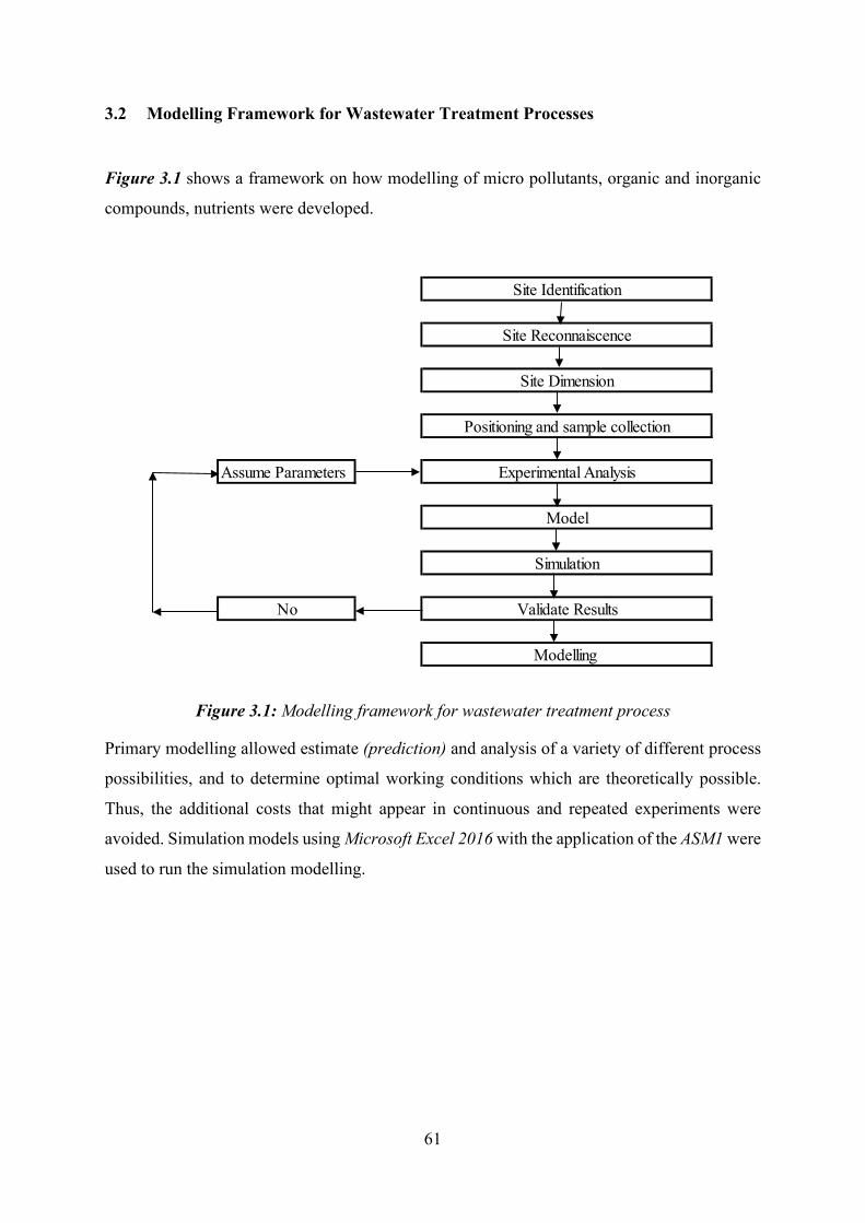
61

3.2 Modelling Framework for Wastewater Treatment Processes

Figure 3.1 shows a framework on how modelling of micro pollutants, organic and inorganic

compounds, nutrients were developed.

Figure 3.1: Modelling framework for wastewater treatment process

Primary modelling allowed estimate (prediction) and analysis of a variety of different process

possibilities, and to determine optimal working conditions which are theoretically possible.

Thus, the additional costs that might appear in continuous and repeated experiments were

avoided. Simulation models using Microsoft Excel 2016 with the application of the ASM1 were

used to run the simulation modelling.

Site Identification

Site Reconnaiscence

Site Dimension

Positioning and sample collection

Assume Parameters Experimental Analysis

Model

Simulation

No Validate Results

Modelling

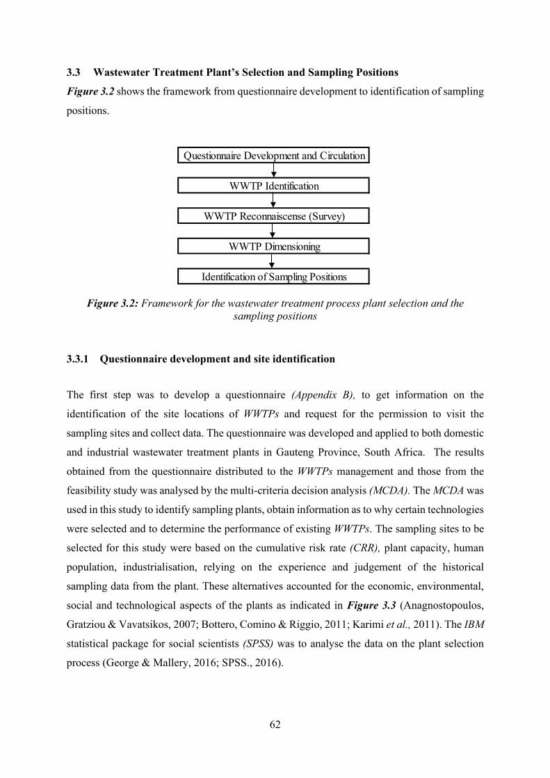
62

3.3 Wastewater Treatment Plant’s Selection and Sampling Positions

Figure 3.2 shows the framework from questionnaire development to identification of sampling

positions.

Figure 3.2: Framework for the wastewater treatment process plant selection and the

sampling positions

3.3.1 Questionnaire development and site identification

The first step was to develop a questionnaire (Appendix B), to get information on the

identification of the site locations of WWTPs and request for the permission to visit the

sampling sites and collect data. The questionnaire was developed and applied to both domestic

and industrial wastewater treatment plants in Gauteng Province, South Africa. The results

obtained from the questionnaire distributed to the WWTPs management and those from the

feasibility study was analysed by the multi-criteria decision analysis (MCDA). The MCDA was

used in this study to identify sampling plants, obtain information as to why certain technologies

were selected and to determine the performance of existing WWTPs. The sampling sites to be

selected for this study were based on the cumulative risk rate (CRR), plant capacity, human

population, industrialisation, relying on the experience and judgement of the historical

sampling data from the plant. These alternatives accounted for the economic, environmental,

social and technological aspects of the plants as indicated in Figure 3.3 (Anagnostopoulos,

Gratziou & Vavatsikos, 2007; Bottero, Comino & Riggio, 2011; Karimi et al., 2011). The IBM

statistical package for social scientists (SPSS) was to analyse the data on the plant selection

process (George & Mallery, 2016; SPSS., 2016).

Questionnaire Development and Circulation

WWTP Identification

WWTP Reconnaiscense (Survey)

WWTP Dimensioning

Identification of Sampling Positions

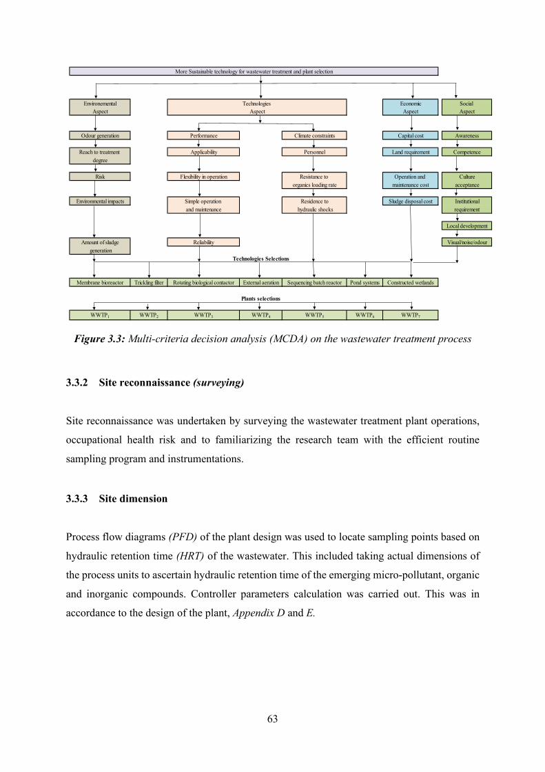
63

Figure 3.3: Multi-criteria decision analysis (MCDA) on the wastewater treatment process

3.3.2 Site reconnaissance (surveying)

Site reconnaissance was undertaken by surveying the wastewater treatment plant operations,

occupational health risk and to familiarizing the research team with the efficient routine

sampling program and instrumentations.

3.3.3 Site dimension

Process flow diagrams (PFD) of the plant design was used to locate sampling points based on

hydraulic retention time (HRT) of the wastewater. This included taking actual dimensions of

the process units to ascertain hydraulic retention time of the emerging micro-pollutant, organic

and inorganic compounds. Controller parameters calculation was carried out. This was in

accordance to the design of the plant, Appendix D and E.

Environemental Economic Social Aspect Aspect Aspect

Odour generation Performance Climate constraints Capital cost Awareness

Reach to treatment Applicability Personnel Land requirement Competencedegree

Risk Flexibility in operation Resistance to Operation and Cultureorganics loading rate maintenance cost acceptance

Environmental impacts Simple operation Residence to Sludge disposal cost Institutionaland maintenance hydraulic shocks requirement

Local development

Amount of sludge Reliability Visual/noise/odour generation

Technologies Selections

Membrane bioreactor Trickling filter Rotating biological contactor External aeration Sequencing batch reactor Pond systems Constructed wetlands

Plants selections

WWTP1 WWTP2 WWTP3 WWTP4 WWTP5 WWTP6 WWTP7

Technologies Aspect

More Sustainable technology for wastewater treatment and plant selection

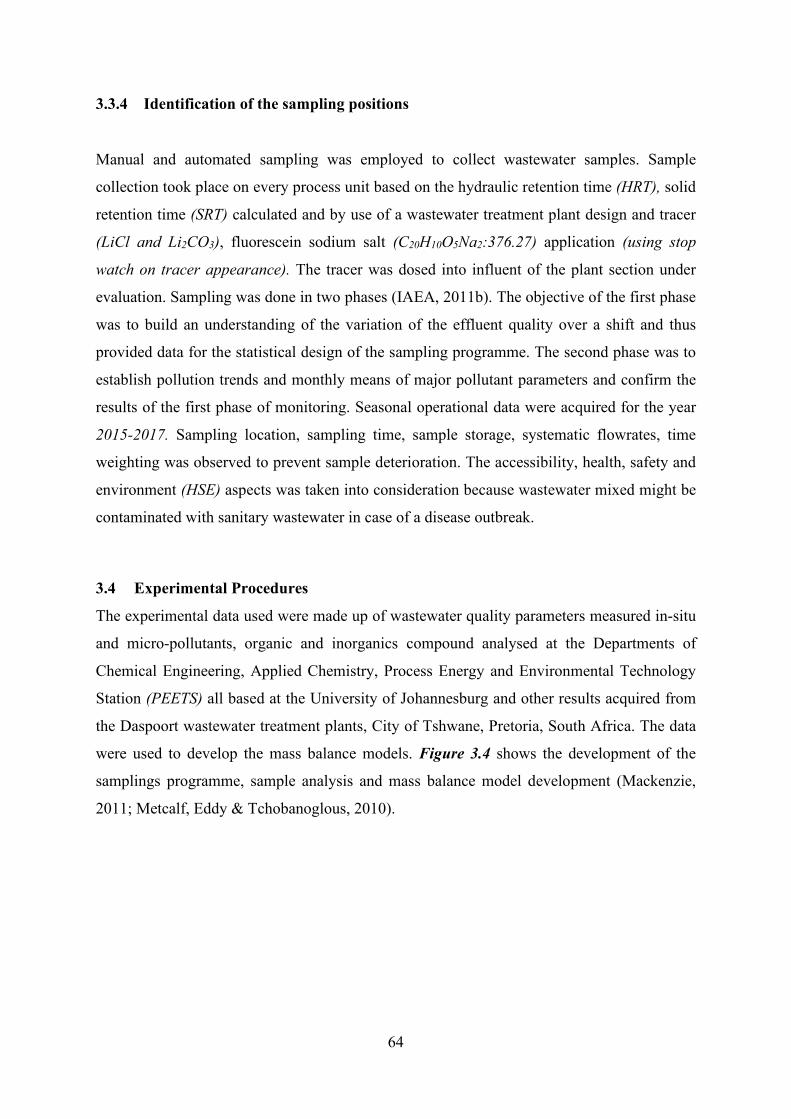
64

3.3.4 Identification of the sampling positions

Manual and automated sampling was employed to collect wastewater samples. Sample

collection took place on every process unit based on the hydraulic retention time (HRT), solid

retention time (SRT) calculated and by use of a wastewater treatment plant design and tracer

(LiCl and Li2CO3), fluorescein sodium salt (C20H10O5Na2:376.27) application (using stop

watch on tracer appearance). The tracer was dosed into influent of the plant section under

evaluation. Sampling was done in two phases (IAEA, 2011b). The objective of the first phase

was to build an understanding of the variation of the effluent quality over a shift and thus

provided data for the statistical design of the sampling programme. The second phase was to

establish pollution trends and monthly means of major pollutant parameters and confirm the

results of the first phase of monitoring. Seasonal operational data were acquired for the year

2015-2017. Sampling location, sampling time, sample storage, systematic flowrates, time

weighting was observed to prevent sample deterioration. The accessibility, health, safety and

environment (HSE) aspects was taken into consideration because wastewater mixed might be

contaminated with sanitary wastewater in case of a disease outbreak.

3.4 Experimental Procedures

The experimental data used were made up of wastewater quality parameters measured in-situ

and micro-pollutants, organic and inorganics compound analysed at the Departments of

Chemical Engineering, Applied Chemistry, Process Energy and Environmental Technology

Station (PEETS) all based at the University of Johannesburg and other results acquired from

the Daspoort wastewater treatment plants, City of Tshwane, Pretoria, South Africa. The data

were used to develop the mass balance models. Figure 3.4 shows the development of the

samplings programme, sample analysis and mass balance model development (Mackenzie,

2011; Metcalf, Eddy & Tchobanoglous, 2010).

65

Figure 3.4: Framework for the development of the samplings programme, sample analysis

and mass balance model

The measured influent organic and inorganic input data (influent wastewater characteristics)

were (American Public Health Association, 2005); total COD, filtered COD, soluble COD,

(after flocculation and filtration), total nitrogen (N), total kjeldahl nitrogen (TKN), ammonia

nitrogen (NH4-N), nitrate/nitrite nitrogen, free and saline ammonia (FSA), total phosphorus

(TP), phosphates (PO43-), volatile fatty acids (VFA), total suspended solids (TSS), chlorine (Cl)

and trace metals. The micro-pollutant analysed were; methylparabens, ethylparabens and

propylparabens. The physical measured data (operation variables) were tank volume, depth

and layouts, flow connections and hydraulic behaviours and flow rates. The performance

measured data were effluent organics, effluent nutrients, mixed liquor (MLSS and MLVSS),

dissolved solids (DO), temperature, pH, alkalinity, ortho phosphate. Second phase objective

was to establish pollution trends and monthly means of major pollutant parameters and confirm

the results of the first phase of monitoring. The accessibility, health, safety and environment

(HSE) aspects was taken into consideration because sometime wastewater is mixed with

sanitary wastewater before discharge to sewer.

3.4.1 Material, chemical and apparatus

3.4.1.1 Material, chemical and apparatus used for the trace metal analysis

Nitric acid was used to adjust the pH of the wastewater before analysis. Fluorescein Sodium

Salt (C20H10O5Na2:376.27), Lithium carbonate (Li2CO3) and lithium chloride (LiCl) was used

as a tracer in the wastewater treatment process. Argon was used as carrier gas for the

inductively coupled plasma optical emission spectrometry (ICP-OES) analysis. Multi-element

standards for trace elements in 100 ppm and 1000 ppm was used for ICP-OES calibration.

Nitric acid and hydrogen peroxide was used for the digestion of the samples prior to trace

elements analysis. The acrodiscs (0.22, 0.45 µm) syringe filters was used to filter the

wastewater samples prior to trace metals analysis.

Development of Sampling Programme

Calibration of the Instruments

Sampling and Analysis (Trace Metals and Organic Compounds)

Mass Balance Modelling

66

3.4.1.2 Reagents and materials used in micro pollutant-organic compounds analysis

The reagents used in the study to derivatize organics in wastewater and for reconstitution of

the final extract included; dichloromethane (DCM), methanol (MeOH), acetonitrile (ACN), n-

hexane formic acid, sodium sulphate and ammonium formate, were all purchased from Sigma-

Aldrich. Solid phase extraction (SPE) cartridges used for extraction of organic compounds in

this study were oasis HLB 500 mg and ENVI-18 500 mg. The acrodiscs (0.22 µm) syringe filters

was used to filter the wastewater samples prior to chromatographic analysis. Reference

analytical standards of the organics, all purchased from Sigma Aldrich for the measurements

of concentrations of analytes in sample solutions included the polycyclic aromatic hydrocarbon

(PAHs); benz[a]antracene, chrysene, acenaphthene, anthracene, naphthalene, pyrene,

organochlorines and organophosphorus, triclosan, disinfection-by-product organics that

included chloroacetic acid, dichloroacetic acid, trichloroacetic acid, and bromoacetic acid.

Deionized water (18 MΩ) was used in making aqueous solutions and standard preparations.

3.4.2 Equipment used for the wastewater analysis

Plastic sample bottles of 500 mL capacity were used to collect samples. Tracer detectors (LiCl

and Li2CO3), fluorescein sodium salt (C20H10O5Na2:376.27), and injector was used to establish

the residence time distribution for the fluid and sludge. A microwave and hotplate were used

in the digestion of the samples. A membrane filter (pore diameter 0.22 µm) was used to filter

the samples before analysis. Inductively coupled plasma optical emission spectrometry (ICP-

OES) was used for trace metals analysis. Organic compounds-micro pollutants were analysed

using gas/liquid chromatograph coupled to various detectors such as the mass spectrometer

(GC-MS and LC-MS) and with high-performance liquid chromatograph (HP-LC) with a UV

detector. Chemical Oxygen Demand (COD) were analysed using spectrophotometer from

Hach. Vials were used to hold liquid samples for analysis. Digital pH meter with electrodes for

measuring temperature and electrical conductivity (EC) were used to analyse pH, temperature

and EC respectively of wastewater treatment on-site.

3.4.3 Computation tools used in simulation modelling

The statistical analysis software package (SPSS) was used to analyse data collected from the

questionnaire for plants selection. Microsoft Excel 2016 was used to run the simulation models,

carry out the mass balance of the wastewater treatment process and preparing graphical

presentations.

67

3.5 Wastewater Sample Preparation and Analysis

3.5.1 Sample source The samples were sourced from Daspoort Wastewater Treatment Plant at City of Tshwane

(CoT) Metro, South Africa, according to the methodology proposed in this study.

3.5.2 Sampling procedure The samples were collected in 500 mL plastic containers, in duplicate, with no headspace

volume to minimise aerobic biodegradation of organics substrates. They were marked with the

indication of time, date and location of collection.

3.5.3 Sample storage The samples were preserved by refrigeration without chemical addition for all the parameters

measured except for trace metals sample to be analysed, where dilute nitric acid was used to

lower the pH to 2 before refrigeration at 4°C. This was to protect trace metals from precipitation

and sorption losses to the container walls (Mackenzie, 2011; Metcalf et al., 2010).

3.5.4 Sample analysis This constitutes sample collection, instrumentation for trace metal and organic compound analysis.

3.5.4.1 On-site analysis

Wastewater electrical conductivity (EC), pH and temperature were measured on-site after

sample collection.

3.5.4.2 Instrumentation for the trace metals analysis

Sample preparation methods for trace metals analysis involved using nitric acid (12 mL) and

hydrogen peroxide (4 mL) for digestion of the sample (10 mL) by hot plate digestion at 120°C

for 2 hours. Deionized water was added to dilute the sample to make 100 mL after digestion.

The sample was then filtered using cellulose acetate membrane filter (0.22 µm). The classes of

metals were: suspended metals, metals present in unacidified samples that are retained on the

0.45 µm membrane filter; dissolved metals, present in unacidified samples that pass through a

0.45 µm membrane filter; total metals, the total of the dissolved and suspended metals or the

concentration of metals determined on an unfiltered sample after digestion, and lastly acid

extractable metals, metals in solution after an unfiltered sample is treated with a hot dilute

mineral acids according to the standard method (Beamish, 2012; Biller & Bruland, 2012).

Calibration standards was prepared using multi-element calibration solutions prepared using-

100 mg/L nitric acid and deionized water. The sample was then analysed using inductively

68

coupled plasma optical emission spectrometry (ICP-OES-model ICAP 6500 Duo) –

(165 Spetro Arcos equipped with autosampler (Cetac ASX-520) technique. The parameters for

operating the ICP-OES was set as follows: instrument power 1400 W, the flow rate of the

auxiliary argon 2 L/min, argon gas flow rate 13 L/min, the flow rate of the argon nebuliser 0.95

L/min and iTEVA software was used. Based on the optical metals wavelength (lower

determination 166.250 nm and extending to 847.000 nm), the most prominent analytical lines

were chosen as follows: Al-396.152 nm, Cd-228.616.502 nm, Co-228.616 nm, Cr-283.565 nm,

Cu-324.754 nm, Fe-259.933 nm, Mn-257.610 nm, Ni-221.647 nm, Pb-220.353 nm, Ti-334.941

nm and Zn-213.856 nm. Dilution factor was applied to the concentration data. The metal of

interest included: Al, Cd, Co, Cr, Cu, Fe, Mn, Mo, Ni, Pb, Ti and Zn (Dimpe, Ngila, Mabuba

& Nomngongo, 2014; Scientific, 2009; Scientific., 2009; Wiel, 2003). Calculation of the

concentration of the elements in the aqueous sample and in the digested solid sample is shown

in (Eq. 3.1 and (Eq. 3.2 respectively (Wiel, 2003).

𝐶𝐶 = (𝐶𝐶1 − 𝐶𝐶𝑜𝑜)𝑜𝑜𝑑𝑑𝑜𝑜𝑎𝑎 Eq. 3.1

𝑤𝑤 = (𝐶𝐶1 − 𝐶𝐶)𝑜𝑜𝑎𝑎𝑉𝑉/𝑀𝑀 Eq. 3.2

Where:

C = concentration of the elements in the aqueous sample in mg/L

C1 = concentration of the elements in the test sample in mg/L

C0 = concentration of the elements in the blank sample in mg/L

fd = dilution factor due to digestion of an aqueous sample; in all other cases fd = 1

fa = dilution factor of the test portion

w = mass fraction of the elements in the solid sample in mg/kg

V = volume of the test sample (digest) in litres

M = mass of the digested sample in g

3.5.4.3 Instrumentation for the organic compound analysis

3.5.4.3.1 Liquid chromatography-mass spectrometry analysis of organics

The liquid chromatographic separation of the organic compounds was performed on a Nexera

UHPLC (Shimadzu corporation, Kyoto, Japan) interfaced to an electrospray-triple quadruple

69

(ESI-QqQ) mass spectrometer and fitted with an ultra-reverse phase biphenyl column (Restek

USA). The separation was achieved on an ultra-reverse phase biphenyl column and C-18

column (Restek, USA). A binary solvent mixture composed of MilliQ water (Mobile phase A)

containing 0.1% formic acid and methanol as mobile phase B was employed for the gradient

elution optimisation and analysis to achieve the analyte separation (Madikizela, Muthwa &

Chimuka, 2014). Stock and working standards solutions of triclosan, haloacetic acids and

parabens was prepared in HPLC grade methanol. A six-point calibration curve for each group

of standards ranging from 5 to 100 μg/L was prepared in the mobile phase. A 1 µg/mL mixed

standard solution was used in optimisation of instrument parameters such as linearity

assessment, column temperature and mass spectrometric operating conditions for maximum

sensitivity. This was done through direct infusion into the mass spectrometer (Paíga et al.,

2015).

3.5.4.3.2 Gas chromatography-mass spectrometry analysis of organics

A two-dimensional gas chromatography time of flight mass spectrometer (GC×GC-TOFMS)

system consisting of an Agilent 7890N GC system (Agilent Technologies, Paloalto, CA, USA)

equipped with an Agilent 7683 autosampler and a single-jet liquid nitrogen cryogenic

modulator and coupled to a Pegasus 4 dimension time-of-flight mass spectrometer (4D TOF)

(LECO Corporation, St. Joseph, MI), operating in the electron ionization (EI) mode, was used

for analysis. This involved screening and quantification of the analytes in the samples after

SPE procedure for analysis of organochlorines and organophosphorus pesticides, and

chlorinated disinfection-by-products (DBPS). The separation was performed using a fused

silica capillary Stabiwax-DA column (29.650 m × 0.32 mm × 0.5 μm, Restek, Bellefonte, PA,

USA). Confirmation of analytes was done by matching the retention times, structures, mass to

charge ratios (m/z) with those on the mass spectrometer (MS) libraries with an accuracy of not

less than 70%. The oven temperature programming for the GC and TOF-MS conditions was

optimised to obtain the most suitable conditions for the analysis. After screening, wastewater

samples identified as having the PAHs, pesticide, and DBPS was re-analysed in triplicate for

quantification purposes using reference calibration standards ranging from 1-100 µg/L

prepared in DCM solution (Skoczyńska, Korytár & Boer, 2008).

3.5.4.3.3 Solid phase extraction of organics in wastewater

The solid phase extraction (SPE) system was optimised to obtain the best extraction conditions

for organics in with good sensitivity and precision. The SPE procedure involved cartridge

70

conditioning, sample loading, analytes isolation and finally elution of the analytes. This was

carried out off-line on a 12-position vacuum manifold (Dimpe & Nomngongo, 2016). The

500 mg C18 SPE cartridges was conditioned by passing 5 mL methanol, 5 mL ethyl acetate:

DCM (50:50), 5 mL methanol and 5 mL water to avoid dryness (Moja & Mtunzi, 2013). The

wastewater samples were filtered before SPE analysis to avoid clogging in the cartridge. A

volume of 500 mL of wastewater sample was loaded automatically through the 500 mg C18

cartridge by use of a vacuum pump. After loading the samples through, the cartridge was

washed with 5 mL deionized water. The cartridge was air-dried, using vacuum for at least 30

min, and then eluted with 5 mL methanol. Where sensitivity was low, the eluate was

concentrated by nitrogen drying and thereafter the pre-concentrated extract was reconstituted

in an appropriate solvent and transferred to sample vials via microfiltration and made ready for

injection on GCXGC-TOFMS or LC-MS/MS (Kanchanamayoon & Tatrahun, 2008; Ma, 2009).

This process was applied to both spiked samples and wastewater samples.

3.5.4.3.4 Liquid-liquid extraction of organics in sludge

The sludge samples were extracted using liquid-liquid extraction followed by pre-

concentration and final analysis. The sludge samples was analysed on a dry weight basis.

Acetone was used in the initial step of extraction with 10 g of dried sample with moderate

shaking for 15 minutes. Thereafter, the acetone extract was subjected to liquid-liquid extraction

by addition of 100 mL deionized water, 20 mL of saturated NaCl solution and 50 mL of

dichloromethane. The organic phase was collected by filtering through a funnel containing

Na2SO4 salt. The sample extract was then pre-concentrated using a rotary evaporator to near

dryness and thereafter reconstituted with 1:9, acetone: hexane or for GCXGC-TOFMS analysis.

For LC-MS/MS analysis the sample was pre-concentrated to dryness and reconstituted in

methanol. Sample extracts were then filtered through 0.22 µm syringe filters prior to

chromatographic analysis (Verlicchi & Zambello, 2015; Zuloaga et al., 2012).

3.5.4.3.5 General standard methods for the wastewater analysis

The measures influent variable: total COD, filtered COD, soluble COD, (after flocculation and

filtration), total nitrogen (N), total kjeldahl nitrogen (TKN), ammonia nitrogen (NH4-N),

nitrate/nitrite nitrogen, free and saline ammonia (FSA), total phosphorus (TP), phosphates

(PO43-), volatile fatty acids (VFA), total suspended solids (TSS), chlorine (Cl) and the

performance measured data: effluent organics, effluent nutrients, mixed liquor (MLSS and

MLVSS), dissolved solids (DO), temperature, pH, alkalinity, ortho phosphate were measured

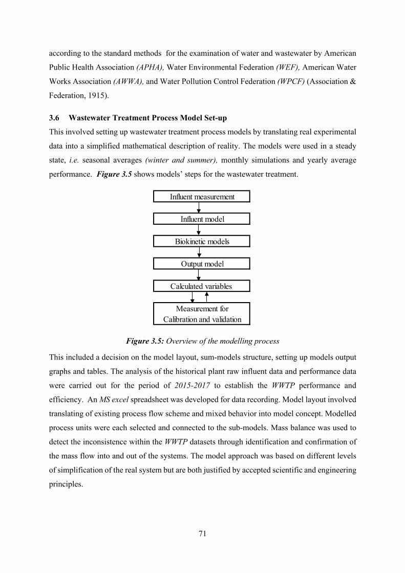
71

according to the standard methods for the examination of water and wastewater by American

Public Health Association (APHA), Water Environmental Federation (WEF), American Water

Works Association (AWWA), and Water Pollution Control Federation (WPCF) (Association &

Federation, 1915).

3.6 Wastewater Treatment Process Model Set-up

This involved setting up wastewater treatment process models by translating real experimental

data into a simplified mathematical description of reality. The models were used in a steady

state, i.e. seasonal averages (winter and summer), monthly simulations and yearly average

performance. Figure 3.5 shows models’ steps for the wastewater treatment.

Figure 3.5: Overview of the modelling process

This included a decision on the model layout, sum-models structure, setting up models output

graphs and tables. The analysis of the historical plant raw influent data and performance data

were carried out for the period of 2015-2017 to establish the WWTP performance and

efficiency. An MS excel spreadsheet was developed for data recording. Model layout involved

translating of existing process flow scheme and mixed behavior into model concept. Modelled

process units were each selected and connected to the sub-models. Mass balance was used to

detect the inconsistence within the WWTP datasets through identification and confirmation of

the mass flow into and out of the systems. The model approach was based on different levels

of simplification of the real system but are both justified by accepted scientific and engineering

principles.

Influent measurement

Influent model

Biokinetic models

Output model

Calculated variables

Measurement forCalibration and validation

72

CHAPTER 4: MATHEMATICAL MODELLING AND MASS BALANCE FOR THE

ORGANIC AND INORGANIC COMPOUNDS IN THE WASTEWATER TREATMENT PROCESSES

4.1 Summary

Wastewater treatment is inherently dynamic because of the large variation in the influent

wastewater concentration, flowrates and composition (i.e. organics, inorganics, and micro-

pollutants). The variations are to a large extent impossible to control in terms of time-varying

process parameters. Mathematical modelling and simulation have become essential to describe,

predict and control the complicated interaction of the wastewater treatment processes. The

study aims to apply mass balance equations and International Association of Water Quality

(IAWQ); Activated Sludge Model (ASM) No.1, abbreviated as ASM1, in the prediction of the

flow rates, organics (substrate and biomass growth), inorganics concentration and their

composition. This combined knowledge of the process dynamics with mathematical methods

for estimation and identification. Emphasis was put on the numerical solution’s ability to

approximate the analytical solution of the conservation law of mass balance. Review on the

existing models were taken into consideration that reached on a consensus concerning the

simplest models having the capability of realistic predictions of the performance of the

activated sludge and biofilm wastewater treatment plant on the nitrification-denitrification,

oxygen demand (DO), pH, alkalinity, phosphorus, temperature, mixed liquor of the suspended

solids, nitrogen, primary settling, sludge retention time, emerging micro pollutants-parabens,

chlorination, and lastly the COD model using the ASM1 and the conventional mass balance in

the course of diurnal variations. The database was analyzed to determine bio-kinetic model’s

parameters range by considering the specific parameters correlation. ASM1 and mass balance

were used as simulation models to simulate the wastewater treatment process. Mass balance

was used to detect the inconsistency within the wastewater treatment plant (WWTP) data sets

through identification and confirmation of the mass flow into and out of the systems. ASM1

facilitated better communication to stakeholders on the complex models that were essential to

the bio-kinetic modelling. Mass balance was a powerful tool that allowed detection of

inconsistencies within the WWTP datasets and assisted in identifying the systematic errors.

Most alternative biological models were influenced by large extent the IAWQ. Calibration of

the models was adjusted with the set of influent data in the process of modification of the input

data until the simulation models result match the dataset. Validation was identified to meet the

73

modelling objectives with the level of confidence. The overall results on the mathematical

modelling of the WWTP formed a framework that could be used in whole plant modelling such

as activated sludge and biofilm models, metabolic approaches, the fate of micro-pollutants and

trace metals reduction processes.

4.2 Introduction

Wastewater treatment processes can be considered as the largest industry in terms of treated

mass of raw materials (Jeppsson, 1996). Wastewater treatment is inherently dynamic because

of the large variation in the influent wastewater concentration, flowrates and composition (i.e.

organics, micro-pollutants and trace metals). The variations are to a large extent impossible to

control in terms of time-varying process parameters. Mathematical modelling and simulation

become essential to describe, predict and control the complicated interaction of the wastewater

treatment processes (Jeppsson, 1996). The models provide an idealized representation of an

actual physical system of the wastewater treatment system (WEF, 2011). Wastewater originates

from domestic wastewater, industrial wastewater, infiltration/inflow, groundwater, stormwater

and surface water. Untreated water results in odour, depletion of dissolved oxygen and the

release of the toxic, nutrients, pathogens and contaminants to the environment. Wastewater is

currently considered as a renewable recoverable source of energy, water and resources.

Wastewater treatment can be achieved by combining a variety of physical (screening, grits,

mixing, flocculation, sedimentation, settling, filtration and adsorption), chemical (oxidation,

coagulation, precipitation, membrane processes, oxidation, gas transfer, adsorption and

disinfection), biological (suspended or attached biomass conversion, nitrification and

denitrification) and thermal (drying, incineration) processes. Micro-organisms are used to

oxidize/convert the particulate and dissolved carbonaceous organic matter into simple end

products. They are also used to remove the nitrogen and phosphorus in wastewater treatment

processes. The major purpose of the secondary treatment is to oxidize the readily biodegradable

COD that escapes primary treatment and provides further removal of the suspended solids and

this includes nitrogen and phosphorus removal (Mackenzie, 2011). Oxygen, phosphate and

ammonia are nutrients needed to the conversion of the organic matter respective simple

products. Biological processes are configured to encourage the growth of bacteria with the

ability to take up and store a large amount of inorganic phosphorus in phosphorus removal.

Ammonia through nitrification is oxidized into nitrite and nitrate. Other bacteria reduce the

oxidized nitrogen into nitrogen gases (Metcalf et al., 2010). The two typical biological

processes for the wastewater treatment are attached growth (biofilm) and the suspended growth.

74

In the attached growth process, the microorganisms are attached to the packing materials (sand,

rocks, gravel, slag, synthetic materials and a wide range of plastic materials) where the organic

matter and nutrients are removed from the wastewater flowing past the attached growth

processes. Attached growth processes can be operated aerobic or anaerobic and mostly referred

to as trickling filters. In the suspended growth processes, the microorganisms responsible for

the treatment are maintained in liquid suspension by appropriate mixing methods. Mostly,

suspended growth in the treatment of industrial and municipality wastewater for biodegradation

of organic matter are operated with dissolved oxygen (aerobic) or nitrate/nitrite (anoxic)

utilization with the support of growth anaerobic (with the absence of oxygen) reactors (Metcalf

et al., 2010). The automation of the wastewater treatment processes instrumentation, control

and automation (ICA) is the best approach to enhancing the efficiency of wastewater treatment

process. Developing countries still use elementary controls which still pose major drawback

up to date. These elementary controls are often fed with off-line data where the on-line sensors

that are both robust and accurate, are either in-line (operating in a side stream) or in-situ

(operating within the process). This is due to; (i) lack of understanding in the treatment

processes and proper understanding of mathematical models; (ii) plant constraints in flexibility

to manipulate the process; (iii) lack of fundamental knowledge concerning benefits versus costs

of the automated treatment processes; (iv) Inadequate instrumentation and reliable technology;

(v) Unsatisfactory communication in designing of the plants among the designers, operators,

researcher, government regulatory agents, equipment manufacturers and supplier; and lastly

(vi) lack of proper training to the operators on how to operate the advanced sensor and control

equipment (Jeppsson, 1996).

Mathematical modelling and simulation have become essential to describe, predict and control

the complicated interaction of the wastewater treatment processes. The study therefore aims to

apply mass balance equations and IAWQ and ASM1, in the prediction of the flow rates,

composition and concentrations of organics which are substrates for biomass growth, and the

composition and concentrations of inorganics.

4.3 Modelling

4.3.1 A State-of-the-Art Model This section provides an overview of activated sludge modelling practice and mass balance of

the suspended and substrate growth of the treatment process of the wastewater. This is with

regards to the theoretical view, reality prediction, history of the models and validation of the

activated sludge modelling. The models’ objectives, structures and construction involve

75

identification, estimation, reduction and validation. The model can be defined as a purposely

representation or description that is often simplified of a system of interest. The model can

present a system that can predict some system behaviours. Mathematical models are used as a

simplification of reality that is relevant to understand and to deal with (Henze, Van Loosdrecht,

Ekama & Brdjanovic, 2008). The mathematical model of activated sludge systems usually

consists of many linked algebraic and differential equation that need to be solved efficiently

under different conditions. These calculations are performed by various algorithms ‘solver’

that form part of the simulator’s numerical ‘engine’. Mathematical models are used for

research, plant optimization, plant designs, training, modelling based development and testing

of the process control (Rieger et al., 2012). A numerical model represents a real-life situation

using mathematical equations. Simulation describes the use of the numerical model within a

software package known as simulator (Rieger et al., 2012). Modelling can be described into

three groups; dynamic state, steady state and frozen state where variation occurs as a function

of time (Henze et al., 2008; Wentzel & Ekama, 1997). Mathematical modelling of the activated

sludge systems has become a widely accepted tool for plants designs, training of the process

operators and engineers, and research tools. According to Rieger et al. (2012), models are only

useful in practice if the model predictions are reliable. For the WWTPs modelling, generally

steady-state and dynamic models are used.

The dynamic models are useful in predicting time-dependent systems response to an existing

or proposed system. Dynamic modelling demand much more stoichiometric and kinetic

constants for the systems design parameters that must be specified. The steady state models

have constant flows and loads and are relatively very simple that their simplicity makes models

very useful for designs.

Steady-state models are useful for calculating the dynamic models such as recycle and waste

flow, reactor volume, concentrations and cross-checking on the simulation models output

(Henze et al., 2008). Modelling of activated sludge processes has become a common part of

the control, operation, research and design. The objective of this study was to mathematically

model wastewater treatment using International Water Association (IWA); Activated Sludge

Models (ASMs) and their practice on application matrix notation of bio-kinetics models and

unified protocols of project definition, data collection and reconciliation, plant model set-up,

calibration/validation and lastly, simulation and results interpretation (Rieger et al., 2012).

Numerical models can be calibrated to one or more data set before applied and then followed

by validation that ensures that the model can be used to predict the behavior of the system

76

under operation. Numerical models can be educational purposes, diagnostic (understanding

mechanisms or processes) or prognostic (predict the future) (Rieger et al., 2012).

Frozen state means that the process changes with time, but not in the time interval that one is

interested in. Usually, the hydraulic retention time is 30 days, resulting in a characteristic time

of change in the digester being in the order of two to three weeks. The process taking place in

a digester can be taken as frozen state. There are processes that are so fast that they are steady

state or are in equilibrium condition. The process occurs so rapidly that the speed of change

exceeds by the dynamics that one is interested in. In the dynamic state, the process is time

varying. Frozen and steady-state processes can be considered continues processes with stable

concentrations under certain conditions like in the digester. The gradient of concentrations

inside the activated sludge floc that can theoretically be described by a model. In a standard

activated sludge modelling it is neglected as being not relevant enough to be considered.

4.3.2 Conventional mathematical modelling The basis for the development of reliable conventional mathematical models is a thorough

understanding of the involved process. Activated sludge systems are usually described by

mathematical models based on the mass balance equations that relate to change of the state

variables of the system (flow rates, concentration and composition) due to transport and the

transformation mechanisms (Jeppsson, 1996).

Activated sludge models (ASMs) are usually not designed to describe the system at the length

scale of an activated sludge floc but at the length scale of a reactor. Modelling of microbial

activity is important although black-box approach focuses on the wastewater treatment plant

influent and effluent characterization with nothing or very litter of microbial activity in the

system. Black-box model can work out well in practice as F/M ratio > ASM1,2,2D > ASM3 >

Metabolic models (Gujer, Henze, Mino & Van Loosdrecht, 1999; Smolders, Van der Meij, Van

Loosdrecht & Heijnen, 1995). The application of black-box models depends very much on the

purpose of the model. One can refine the approach of the plant design towards grey-box models

as activated sludge model 1 (ASM1), Activated sludge model 2, 2d (ASM2, 2d) and Activated

sludge 3 (ASM3) (Henze et al., 2002). The metabolism of the organisms and metabolic routes

inside the organism is described by glass-box modelling such as ASM3, TU Delft EBPR model

(TUDP model) (Henze et al., 2008; Van Veldhuizen, Van Loosdrecht & Heijnen, 2015). A

brief history of the wastewater models was based on BOD and mixed liquor suspended solids

(MLSS) UCT in 60s and carbon and nitrogen removal in 1983 ASM1 (Henze, Grady, Gujer,

Marais & Matsuo, 1987; Henze et al., 2002). The bio-phosphorus (bio-P) removal included

77

ASM2 (Rieger et al., 2012), Barker and Dold (Barker & Dold, 1997) and ASM2d (Henze et al.,

1999). The new concept of the C and N removal (ASM3) (Gujer et al., 1999), ASM3+Bio-P

(EAWAG) (Rieger, Koch, Kühni, Gujer & Siegrist, 2001), UCTPHO+ (Hauduc et al., 2010;

Hu, Wentzel & Ekama, 2007), metabolic model (Delft University) and elemental balances

(Takács & Vanrolleghem, 2006). Academic wastewater treatment models are characterized as

ASM1/2/2d/3, ASM3+Bio-P, Barker and Bold, UCTPHO+, TUDelft, etc. The engineering

models are integrated into commercial simulators, i.e. AQUASIM, BIOWIN, GPSX,

STROAT, SIMBA, WEST, MATLAB SIMULINK, SUMO, CHEMCAD, ASPEN PLUS,

BALAS, DTS PRO, DYNOCHEM, etc. (Committee, 2013). The ASM1 database contains 31

parameters set, where 22 are optimized parameters sets, and 9 are proposed new default

parameters (Rieger et al., 2012).

Steady-state and dynamic models are the mathematic models that describe wastewater

treatment systems. Steady state model simplicity makes them relatively simple to use in design

and process efficiency determination due to constant flows and loading rate. Dynamic models

are useful in prediction time-dependent systems response of an existing or proposed system.

Dynamic model guide in the development of the steady-state design models by identifying the

design parameters that have a major influence on the system response (Henze et al., 2008).

Wastewater treatment plant models are used to indicate the ensemble of the activated sludge

models, oxygen transfer model, hydraulic model and sedimentation tank model (Gernaey, Van

Loosdrecht, Henze, Lind & Jørgensen, 2004).

4.4 Experimental Procedures

The mathematical modelling-mass balance project was undertaken at Plant A Wastewater

treatment plant, South Africa. Models show the capability of realistic predictions of the

performance of the activated sludge and biofilm wastewater treatment plant on the nitrification-

denitrification, oxygen demand (DO), pH, alkalinity, phosphorus, temperature, mixed liquor of

the suspended solids, nitrogen, primary settling, sludge retention time, emerging micro

pollutants-parabens, chlorination, and lastly the COD model using the ASM1 and the

conventional mass balance in the course of diurnal variations.

4.4.1 Mass balance of wastewater treatment plant

Mass balance is an engineering tool that allowed the identification and confirmation of the

mass flow into and out of a processing system based on a mass conservation principle. Open

and closed mass balance was applied. The measured influent organic and suspended input data

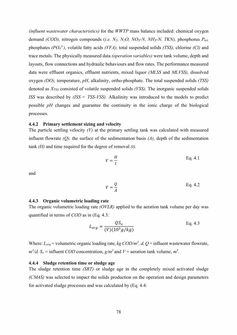
78

(influent wastewater characteristics) for the WWTP mass balance included: chemical oxygen

demand (COD), nitrogen compounds (i.e. N2, N2O, NOX-N, NHX-N, TKN), phosphorus Ptot,

phosphates (PO43-), volatile fatty acids (VFA), total suspended solids (TSS), chlorine (Cl) and

trace metals. The physically measured data (operation variables) were tank volume, depth and

layouts, flow connections and hydraulic behaviours and flow rates. The performance measured

data were effluent organics, effluent nutrients, mixed liquor (MLSS and MLVSS), dissolved

oxygen (DO), temperature, pH, alkalinity, ortho-phosphate. The total suspended solids (TSS)

denoted as XTSS consisted of volatile suspended solids (VSS). The inorganic suspended solids

ISS was described by (ISS = TSS-VSS). Alkalinity was introduced to the models to predict

possible pH changes and guarantee the continuity in the ionic charge of the biological

processes.

4.4.2 Primary settlement sizing and velocity The particle settling velocity (V) at the primary settling tank was calculated with measured

influent flowrate (Q), the surface of the sedimentation basis (A), depth of the sedimentation

tank (H) and time required for the degree of removal (t).

𝑉𝑉 =𝐻𝐻𝑡𝑡

Eq. 4.1

and

𝑉𝑉 =𝑄𝑄𝐴𝐴

Eq. 4.2

4.4.3 Organic volumetric loading rate The organic volumetric loading rate (OVLR) applied to the aeration tank volume per day was

quantified in terms of COD as in (Eq. 4.3:

𝐿𝐿𝑜𝑜𝑜𝑜𝑜𝑜 =𝑄𝑄𝑆𝑆𝑜𝑜

(𝑉𝑉)(103𝑔𝑔/𝑘𝑘𝑔𝑔)

Eq. 4.3

Where: Lorg = volumetric organic loading rate, kg COD/m3. d, Q = influent wastewater flowrate,

m3/d, So = influent COD concentration, g/m3 and V = aeration tank volume, m3.

4.4.4 Sludge retention time or sludge age The sludge retention time (SRT) or sludge age in the completely mixed activated sludge

(CMAS) was selected to impact the solids production on the operation and design parameters

for activated sludge processes and was calculated by (Eq. 4.4:

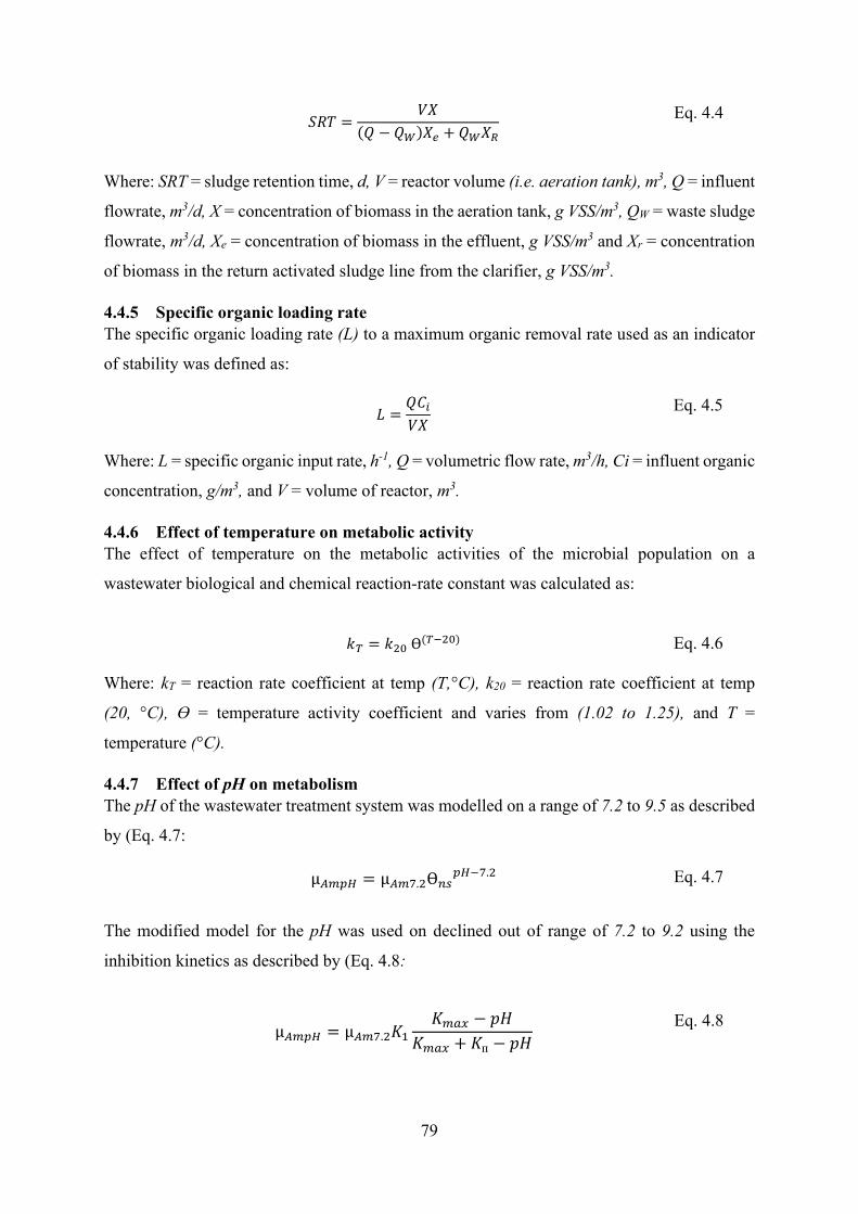
79

𝑆𝑆𝑅𝑅𝑅𝑅 =𝑉𝑉𝑉𝑉

(𝑄𝑄 − 𝑄𝑄𝑊𝑊)𝑉𝑉𝑒𝑒 + 𝑄𝑄𝑊𝑊𝑉𝑉𝑅𝑅 Eq. 4.4

Where: SRT = sludge retention time, d, V = reactor volume (i.e. aeration tank), m3, Q = influent

flowrate, m3/d, X = concentration of biomass in the aeration tank, g VSS/m3, QW = waste sludge

flowrate, m3/d, Xe = concentration of biomass in the effluent, g VSS/m3 and Xr = concentration

of biomass in the return activated sludge line from the clarifier, g VSS/m3.

4.4.5 Specific organic loading rate The specific organic loading rate (L) to a maximum organic removal rate used as an indicator

of stability was defined as:

𝐿𝐿 =𝑄𝑄𝐶𝐶𝑖𝑖𝑉𝑉𝑉𝑉

Eq. 4.5

Where: L = specific organic input rate, h-1, Q = volumetric flow rate, m3/h, Ci = influent organic

concentration, g/m3, and V = volume of reactor, m3.

4.4.6 Effect of temperature on metabolic activity The effect of temperature on the metabolic activities of the microbial population on a

wastewater biological and chemical reaction-rate constant was calculated as:

𝑘𝑘𝑇𝑇 = 𝑘𝑘20 Ɵ(𝑇𝑇−20)

Eq. 4.6

Where: kT = reaction rate coefficient at temp (T,°C), k20 = reaction rate coefficient at temp

(20, °C), Ɵ = temperature activity coefficient and varies from (1.02 to 1.25), and T =

temperature (°C).

4.4.7 Effect of pH on metabolism The pH of the wastewater treatment system was modelled on a range of 7.2 to 9.5 as described

by (Eq. 4.7:

µ𝐴𝐴𝐴𝐴𝐴𝐴𝐴𝐴 = µ𝐴𝐴𝐴𝐴7.2Ɵ𝑛𝑛𝑛𝑛𝐴𝐴𝐴𝐴−7.2

Eq. 4.7

The modified model for the pH was used on declined out of range of 7.2 to 9.2 using the

inhibition kinetics as described by (Eq. 4.8:

µ𝐴𝐴𝐴𝐴𝐴𝐴𝐴𝐴 = µ𝐴𝐴𝐴𝐴7.2𝐾𝐾1𝐾𝐾𝐴𝐴𝑎𝑎𝑚𝑚 − 𝑝𝑝𝐻𝐻

𝐾𝐾𝐴𝐴𝑎𝑎𝑚𝑚 + 𝐾𝐾п − 𝑝𝑝𝐻𝐻

Eq. 4.8

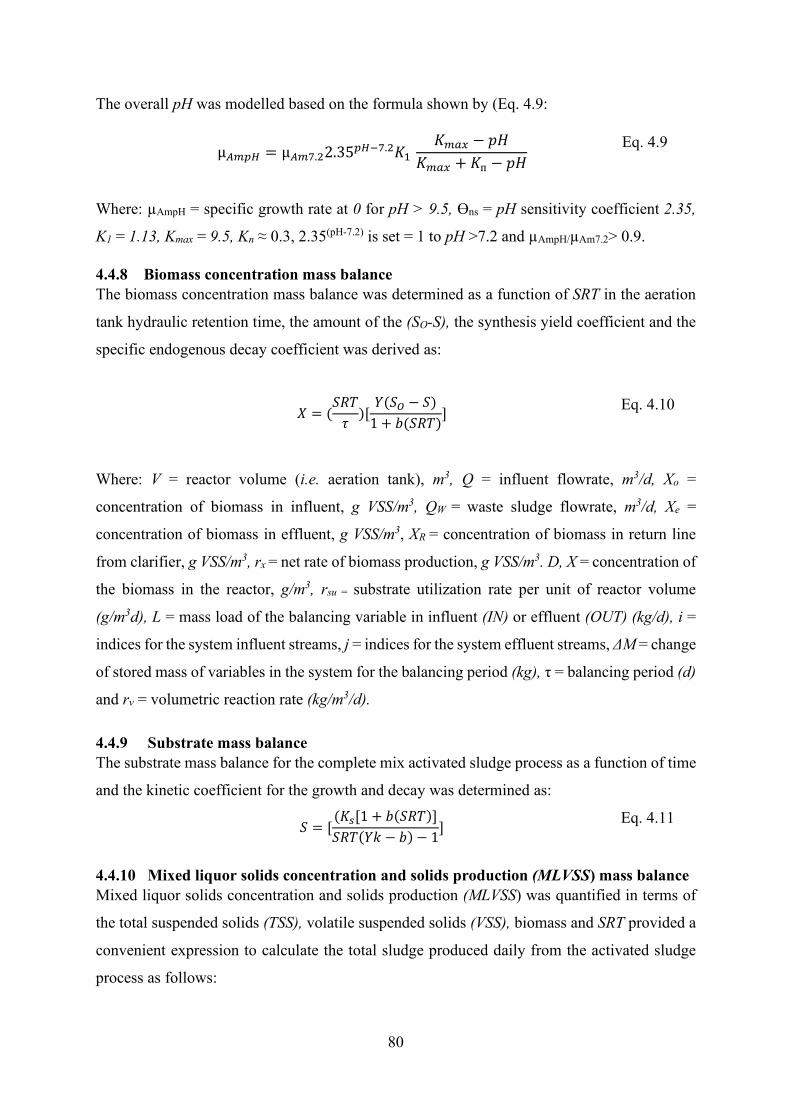
80

The overall pH was modelled based on the formula shown by (Eq. 4.9:

µ𝐴𝐴𝐴𝐴𝐴𝐴𝐴𝐴 = µ𝐴𝐴𝐴𝐴7.22.35𝐴𝐴𝐴𝐴−7.2𝐾𝐾1 𝐾𝐾𝐴𝐴𝑎𝑎𝑚𝑚 − 𝑝𝑝𝐻𝐻

𝐾𝐾𝐴𝐴𝑎𝑎𝑚𝑚 + 𝐾𝐾п − 𝑝𝑝𝐻𝐻

Eq. 4.9

Where: µAmpH = specific growth rate at 0 for pH > 9.5, Ɵns = pH sensitivity coefficient 2.35,

K1 = 1.13, Kmax = 9.5, Kп ≈ 0.3, 2.35(pH-7.2) is set = 1 to pH >7.2 and µAmpH/µAm7.2> 0.9.

4.4.8 Biomass concentration mass balance The biomass concentration mass balance was determined as a function of SRT in the aeration

tank hydraulic retention time, the amount of the (SO-S), the synthesis yield coefficient and the

specific endogenous decay coefficient was derived as:

𝑉𝑉 = (𝑆𝑆𝑅𝑅𝑅𝑅𝜏𝜏

)[𝑌𝑌(𝑆𝑆𝑂𝑂 − 𝑆𝑆)

1 + 𝑏𝑏(𝑆𝑆𝑅𝑅𝑅𝑅)] Eq. 4.10

Where: V = reactor volume (i.e. aeration tank), m3, Q = influent flowrate, m3/d, Xo =

concentration of biomass in influent, g VSS/m3, QW = waste sludge flowrate, m3/d, Xe =

concentration of biomass in effluent, g VSS/m3, XR = concentration of biomass in return line

from clarifier, g VSS/m3, rx = net rate of biomass production, g VSS/m3. D, X = concentration of

the biomass in the reactor, g/m3, rsu = substrate utilization rate per unit of reactor volume

(g/m3d), L = mass load of the balancing variable in influent (IN) or effluent (OUT) (kg/d), i =

indices for the system influent streams, j = indices for the system effluent streams, ΔM = change

of stored mass of variables in the system for the balancing period (kg), τ = balancing period (d)

and rv = volumetric reaction rate (kg/m3/d).

4.4.9 Substrate mass balance The substrate mass balance for the complete mix activated sludge process as a function of time

and the kinetic coefficient for the growth and decay was determined as:

𝑆𝑆 = [(𝐾𝐾𝑛𝑛[1 + 𝑏𝑏(𝑆𝑆𝑅𝑅𝑅𝑅)]𝑆𝑆𝑅𝑅𝑅𝑅(𝑌𝑌𝑘𝑘 − 𝑏𝑏) − 1

]

Eq. 4.11

4.4.10 Mixed liquor solids concentration and solids production (MLVSS) mass balance Mixed liquor solids concentration and solids production (MLVSS) was quantified in terms of

the total suspended solids (TSS), volatile suspended solids (VSS), biomass and SRT provided a

convenient expression to calculate the total sludge produced daily from the activated sludge

process as follows:

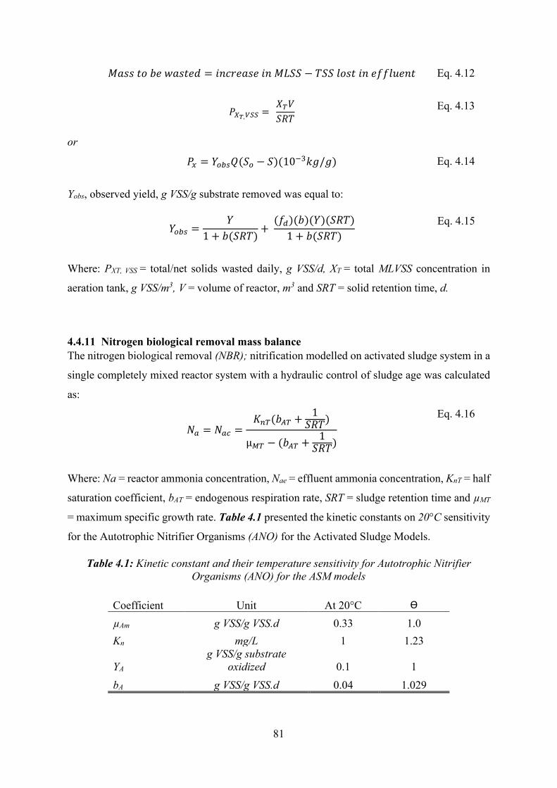
81

𝑀𝑀𝑟𝑟𝑀𝑀𝑀𝑀 𝑡𝑡𝑜𝑜 𝑏𝑏𝑟𝑟 𝑤𝑤𝑟𝑟𝑀𝑀𝑡𝑡𝑟𝑟𝑑𝑑 = 𝑟𝑟𝑟𝑟𝑟𝑟𝑟𝑟𝑟𝑟𝑟𝑟𝑀𝑀𝑟𝑟 𝑟𝑟𝑟𝑟 𝑀𝑀𝐿𝐿𝑆𝑆𝑆𝑆 − 𝑅𝑅𝑆𝑆𝑆𝑆 𝑙𝑙𝑜𝑜𝑀𝑀𝑡𝑡 𝑟𝑟𝑟𝑟 𝑟𝑟𝑜𝑜𝑜𝑜𝑙𝑙𝑒𝑒𝑟𝑟𝑟𝑟𝑡𝑡

Eq. 4.12

𝑃𝑃𝑋𝑋𝑇𝑇,𝑉𝑉𝑉𝑉𝑉𝑉 = 𝑉𝑉𝑇𝑇𝑉𝑉𝑆𝑆𝑅𝑅𝑅𝑅

Eq. 4.13

or

𝑃𝑃𝑚𝑚 = 𝑌𝑌𝑜𝑜𝑜𝑜𝑛𝑛𝑄𝑄(𝑆𝑆𝑜𝑜 − 𝑆𝑆)(10−3𝑘𝑘𝑔𝑔/𝑔𝑔)

Eq. 4.14

Yobs, observed yield, g VSS/g substrate removed was equal to:

𝑌𝑌𝑜𝑜𝑜𝑜𝑛𝑛 =

𝑌𝑌1 + 𝑏𝑏(𝑆𝑆𝑅𝑅𝑅𝑅)

+ (𝑜𝑜𝑑𝑑)(𝑏𝑏)(𝑌𝑌)(𝑆𝑆𝑅𝑅𝑅𝑅)

1 + 𝑏𝑏(𝑆𝑆𝑅𝑅𝑅𝑅)

Eq. 4.15

Where: PXT, VSS = total/net solids wasted daily, g VSS/d, XT = total MLVSS concentration in

aeration tank, g VSS/m3, V = volume of reactor, m3 and SRT = solid retention time, d.

4.4.11 Nitrogen biological removal mass balance The nitrogen biological removal (NBR); nitrification modelled on activated sludge system in a

single completely mixed reactor system with a hydraulic control of sludge age was calculated

as:

𝑁𝑁𝑎𝑎 = 𝑁𝑁𝑎𝑎𝑐𝑐 =

𝐾𝐾𝑛𝑛𝑇𝑇(𝑏𝑏𝐴𝐴𝑇𝑇 + 1𝑆𝑆𝑅𝑅𝑅𝑅)

µ𝑀𝑀𝑇𝑇 − (𝑏𝑏𝐴𝐴𝑇𝑇 + 1𝑆𝑆𝑅𝑅𝑅𝑅)

Eq. 4.16

Where: Na = reactor ammonia concentration, Nae = effluent ammonia concentration, KnT = half

saturation coefficient, bAT = endogenous respiration rate, SRT = sludge retention time and µMT

= maximum specific growth rate. Table 4.1 presented the kinetic constants on 20°C sensitivity

for the Autotrophic Nitrifier Organisms (ANO) for the Activated Sludge Models.

Table 4.1: Kinetic constant and their temperature sensitivity for Autotrophic Nitrifier Organisms (ANO) for the ASM models

Coefficient Unit At 20°C Ɵ

µAm g VSS/g VSS.d 0.33 1.0 Kn mg/L 1 1.23

YA g VSS/g substrate

oxidized 0.1 1 bA g VSS/g VSS.d 0.04 1.029

82

In order to be able to compare the data collected at different temperature in nitrification, all the

kinetic constants were corrected to a standard value of 20°C (temperature dependencies).

µ𝐴𝐴𝑇𝑇 = µ𝐴𝐴20. 1.0123(𝑇𝑇−20)

Eq. 4.17

𝑏𝑏𝐴𝐴𝑇𝑇 = 𝑏𝑏𝐴𝐴20. 1.0123(𝑇𝑇−20)

Eq. 4.18

𝐾𝐾𝑛𝑛𝑇𝑇 = 𝐾𝐾𝑛𝑛20. 1.0123(𝑇𝑇−20)

Eq. 4.19

𝑁𝑁𝑟𝑟𝑡𝑡𝑟𝑟𝑜𝑜𝑔𝑔𝑟𝑟𝑟𝑟 𝑜𝑜𝑜𝑜𝑟𝑟𝑑𝑑𝑟𝑟𝑀𝑀𝑟𝑟𝑑𝑑

= 𝑁𝑁𝑟𝑟𝑡𝑡𝑟𝑟𝑜𝑜𝑔𝑔𝑟𝑟𝑟𝑟 𝑟𝑟𝑟𝑟 𝑟𝑟𝑟𝑟𝑜𝑜𝑙𝑙𝑒𝑒𝑟𝑟𝑟𝑟𝑡𝑡 − 𝑁𝑁𝑟𝑟𝑡𝑡𝑟𝑟𝑜𝑜𝑔𝑔𝑟𝑟𝑟𝑟 𝑟𝑟𝑟𝑟 𝑟𝑟𝑜𝑜𝑜𝑜𝑙𝑙𝑒𝑒𝑟𝑟𝑟𝑟𝑡𝑡 − 𝑁𝑁𝑟𝑟𝑡𝑡𝑟𝑟𝑜𝑜𝑔𝑔𝑟𝑟𝑟𝑟 𝑟𝑟𝑟𝑟 𝑟𝑟𝑟𝑟𝑙𝑙𝑙𝑙 𝑡𝑡𝑟𝑟𝑀𝑀𝑀𝑀𝑒𝑒𝑟𝑟

Eq. 4.20

𝑁𝑁𝑁𝑁𝑋𝑋 = 𝑅𝑅𝐾𝐾𝑁𝑁𝑂𝑂 − 𝑁𝑁𝑒𝑒 − 0.12(𝑃𝑃𝑋𝑋𝑄𝑄

)

Eq. 4.21

Where: NOX = nitrogen oxidized, mg/L, TKNO = influent total Kjeldahl nitrogen, mg/L, and Ne

= effluent NH4-N, mg/L.

4.4.12 Biological phosphorus removal In the biological phosphorus removal (BPR), the total discharge or organic phosphorus with

the effluent was determined by the following equation:

𝑃𝑃𝑜𝑜𝐴𝐴𝑒𝑒 = 𝑜𝑜𝐴𝐴.𝑉𝑉𝑣𝑣𝑒𝑒 = 𝑜𝑜𝐴𝐴. 𝑜𝑜𝑣𝑣.𝑉𝑉𝑡𝑡𝑒𝑒

Eq. 4.22

Where: Ppe = inorganic phosphate, Poe = organic phosphorus, Pose = soluble organic

phosphorus, typically between 0.1 and 0.2 mg P.1-1, fp = phosphate residual (0.025 g P. g-1

VSS), Xve = concentration of VSS, fv = VSS residual, typically between (0.70 to 0.85 VSS .mg-1

TSS), and Xte = concentration of VSS.

The phosphate release in the anaerobic zone in the presence of an adequate (VFA, such as

acetate), the bio-P organisms transform internally stored polyphosphate into phosphate, a

process that releases the energy required for the absorption of VFA was determined by the

following equation:

83

𝑃𝑃𝑜𝑜 = 𝑜𝑜𝐴𝐴𝑜𝑜 . 𝑆𝑆𝑉𝑉𝑑𝑑𝐴𝐴

Eq. 4.23

Where: Pr = phosphate concentration released to the liquid phase (mg P.1-1), SVFA =

concentration of the volatile fatty acids (mg COD.1-1) and fpr = phosphorus release constant =

0.5 mg P. mg-1 COD absorbed.

4.4.13 Oxygen demand mass balance The oxygen required for the biodegradation of carbonaceous material was determined from a

mass balance using bCOD concentration of the wastewater treated and the amount of biomass

wasted from the system per day:

𝑅𝑅𝑂𝑂 = 𝑄𝑄(𝑆𝑆𝑂𝑂 − 𝑆𝑆) − 1.42𝑃𝑃𝑋𝑋,𝑜𝑜𝑖𝑖𝑜𝑜

Eq. 4.24

Where: Ro = oxygen required, kg/d, Q = wastewater flow rate into the aeration tank, m3/d, So =

influent bCOD, g/m3, S = effluent bCOD, g/m3, and Px, bio = biomass as VSS wasted per day,

(waste activated sludge produced) kg/d.

Dissolved oxygen concentration was formulated as follows:

µ𝐴𝐴𝑂𝑂 = µ𝐴𝐴𝐴𝐴𝑂𝑂𝑁𝑁2

𝐾𝐾𝑜𝑜 − 𝑁𝑁2

Eq. 4.25

Where: µAo = maximum specific growth rate (/d), µAmO = specific growth rate at DO of O

(mg/L), O2 = oxygen concentration in liquid (mgO2/L), and Ko = half saturation constant

(mgO2/L), range 0.3-2.

4.4.14 Biological removal of recalcitrant and trace organic compounds The mass balance for the biological removal of emerging organic compounds (emerging micro-

pollutants) resists conventional biodegradation in biological treatment processes referred to as

refractory (methylparabens, ethylparabens, propylparabens) was represented by:

𝑆𝑆 = [(𝐾𝐾𝑛𝑛[1 + 𝑏𝑏(𝑆𝑆𝑅𝑅𝑅𝑅)]𝑆𝑆𝑅𝑅𝑅𝑅�µ𝑚𝑚 − 𝑏𝑏� − 1

]

Eq. 4.26

Where: QSo = mass of the compounds in wastewater influent, g/d, rsu = biodegradation rate,

g/d, rad = solid adsorption rate, g/d, rrv = volatilization rate, g/d, QS = mass of compounds in

wastewater effluent, g/d, Q = hydraulic flow rate (m3/d), V = Aeration tank volume, m3, SO =

84

influent concentration (mg/L), S = effluent concentration (mg/L), SRT = solid retention time,

XT = total MLVSS concentration that includes all the biomass grown on various substrates plus

the nonbiodegradable VSS, XS = biomass concentration capable of degrading the specific

organic compounds, Y = synthesis yield coefficient, g biomass/g substrate used, KL as = gas-

liquid mass transfer coefficient, of organic compound, d , KP = partition coefficient, (L/g), τ =

aeration tank retention time (hydraulic retention time) and µm = maximum specific growth rate

(g/g.d).

4.4.15 Disinfectants used in the wastewater treatment Pathogens (fungi, viruses, helminth, protozoan oocysts, bacteria) were removed in the effluent

by the application of disinfectants; chlorine. The chemical disinfectant kinetics of the chlorine

was based on the pseudo-first order decay rate constants are shown below (Mackenzie, 2011;

U.S EPA, 1986):

𝐶𝐶 = 𝐶𝐶𝑂𝑂𝑟𝑟𝑜𝑜𝑝𝑝(−𝑘𝑘𝑑𝑑𝑡𝑡)

Eq. 4.27

Where: C = disinfectant concentration, mg/L, kd = first order decay rate constant, time-1 (0.0011

to 0.0101 min-1 surface water with the TOC of 2.3 to 3.8 mg/L, 0.71 to 11.09 d-1 distribution

system pipe, and 0.36 to 1.0 d-1 for distribution system storage tank, t = time, and

complementary units to kd.

4.4.16 Food to microorganism ratio Food to microorganism (F/M) ratio was defined as the rate of COD and applied per unit mixed

liquor as:

𝐹𝐹𝑀𝑀

=𝑅𝑅𝑜𝑜𝑡𝑡𝑟𝑟𝑙𝑙 𝑟𝑟𝑝𝑝𝑝𝑝𝑙𝑙𝑟𝑟𝑟𝑟𝑑𝑑 𝑀𝑀𝑒𝑒𝑏𝑏𝑀𝑀𝑡𝑡𝑟𝑟𝑟𝑟𝑡𝑡𝑟𝑟 𝑟𝑟𝑟𝑟𝑡𝑡𝑟𝑟𝑅𝑅𝑜𝑜𝑡𝑡𝑟𝑟𝑙𝑙 𝑚𝑚𝑟𝑟𝑟𝑟𝑟𝑟𝑜𝑜𝑏𝑏𝑟𝑟𝑟𝑟𝑙𝑙 𝑏𝑏𝑟𝑟𝑜𝑜𝑚𝑚𝑟𝑟𝑀𝑀𝑀𝑀

=𝑄𝑄𝑆𝑆𝑂𝑂𝑉𝑉𝑉𝑉

=𝑆𝑆𝑂𝑂𝜏𝜏𝑉𝑉

Eq. 4.28

Where: F/M = food to biomass ratio, bsCOD/g VSS.d, Q = influent wastewater flowrate into

the aeration tank, m3/d, So = influent biodegradable soluble bsCOD concentration, mg/L, X =

mixed liquor biomass concentration in the aeration tank, mg/L and τ = hydraulic retention time

of aeration tank, V/Q, d.

85

4.4.17 Removal efficiency of the organic compounds’ removal The process removal efficiency (E) as percent COD across the activated sludge system was

defined by:

𝐸𝐸 =𝑆𝑆𝑜𝑜 − 𝑆𝑆𝑆𝑆𝑜𝑜

(100)

Eq. 4.29

4.4.18 Calibration and validation Mathematical models were introduced at elucidating the mechanisms of the activated sludge

processes. Calibration of the models were adjusted with the set of influent experimental data

in the process of modification of the input data until the simulation model results match the

data set. The effluent results were counter checked for compliance with Department of Water;

wastewater treatment License, Appendix D. Validation was identified to meet the modelling

objectives with the level of confidence.

4.5 Results and Discussions

4.5.1 Modelling analysis using microbial growth kinetics, mass balance, and activated sludge model No. 1 of the WWTP The key objective for developing a model of the wastewater system included obtaining reliable

measurements (observation), the selection of the key behaviour and characteristic,

approximations and assumptions, the accuracy of the simulation model output

(calibration/validation) and realistic of the predictions. Mass balance was a powerful tool that

allowed detection of inconsistencies within the WWTP data sets and assists to identify the

systematic errors. Mass balance was carried under steady state to identify potential data

sampling and analytical errors monitoring. Steady-state modelling was again essential for plant

performance under various loading conditions and for future WWTP design and redesign. The

steady state satisfied the long-term behaviour of the flow rate and where there was no

significant inherent dynamics. The setting up of the influent characteristic was calibrated prior

to the kinetic parameters and the influent characteristics. According to Rieger et al. (2012),

mass balance does not provide information on the precision of a specific measurement. It was

possible to identify mass balance based on many variables that were set up of parallel mass

balance utilizing process variables. This was useful in identifying systematic measuring errors

in the overlapping mass balance. The rule of thumb expected for the mass balance on the data

was average 7%, close to residual in a range of ±5 to 10% (Rieger et al., 2012). All the models

were benchmarked according to the IWA task group on the control strategies of the WWTP

(IWA, [(Accessed February 2018]).

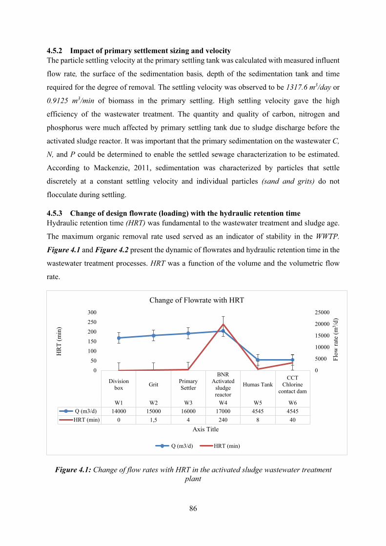
86

4.5.2 Impact of primary settlement sizing and velocity The particle settling velocity at the primary settling tank was calculated with measured influent

flow rate, the surface of the sedimentation basis, depth of the sedimentation tank and time

required for the degree of removal. The settling velocity was observed to be 1317.6 m3/day or

0.9125 m3/min of biomass in the primary settling. High settling velocity gave the high

efficiency of the wastewater treatment. The quantity and quality of carbon, nitrogen and

phosphorus were much affected by primary settling tank due to sludge discharge before the

activated sludge reactor. It was important that the primary sedimentation on the wastewater C,

N, and P could be determined to enable the settled sewage characterization to be estimated.

According to Mackenzie, 2011, sedimentation was characterized by particles that settle

discretely at a constant settling velocity and individual particles (sand and grits) do not

flocculate during settling.

4.5.3 Change of design flowrate (loading) with the hydraulic retention time Hydraulic retention time (HRT) was fundamental to the wastewater treatment and sludge age.

The maximum organic removal rate used served as an indicator of stability in the WWTP.

Figure 4.1 and Figure 4.2 present the dynamic of flowrates and hydraulic retention time in the

wastewater treatment processes. HRT was a function of the volume and the volumetric flow

rate.

Figure 4.1: Change of flow rates with HRT in the activated sludge wastewater treatment plant

Divisionbox Grit Primary

Settler

BNRActivated

sludgereactor

Humas TankCCT

Chlorinecontact dam

W1 W2 W3 W4 W5 W6 Q (m3/d) 14000 15000 16000 17000 4545 4545HRT (min) 0 1,5 4 240 8 40

050

100

150200250300

0

5000

10000

15000

20000

25000

HR

T (m

in)

Axis Title

Flow

rate

(m3 /d

)

Change of Flowrate with HRT

Q (m3/d) HRT (min)

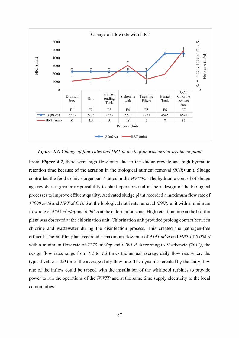
87

Figure 4.2: Change of flow rates and HRT in the biofilm wastewater treatment plant

From Figure 4.2, there were high flow rates due to the sludge recycle and high hydraulic

retention time because of the aeration in the biological nutrient removal (BNR) unit. Sludge

controlled the food to microorganisms’ ratios in the WWTPs. The hydraulic control of sludge

age revolves a greater responsibility to plant operators and in the redesign of the biological

processes to improve effluent quality. Activated sludge plant recorded a maximum flow rate of

17000 m3/d and HRT of 0.16 d at the biological nutrients removal (BNR) unit with a minimum

flow rate of 4545 m3/day and 0.005 d at the chlorination zone. High retention time at the biofilm

plant was observed at the chlorination unit. Chlorination unit provided prolong contact between

chlorine and wastewater during the disinfection process. This created the pathogen-free

effluent. The biofilm plant recorded a maximum flow rate of 4545 m3/d and HRT of 0.006 d

with a minimum flow rate of 2273 m3/day and 0.001 d. According to Mackenzie (2011), the

design flow rates range from 1.2 to 4.3 times the annual average daily flow rate where the

typical value is 2.0 times the average daily flow rate. The dynamics created by the daily flow

rate of the inflow could be tapped with the installation of the whirlpool turbines to provide

power to run the operations of the WWTP and at the same time supply electricity to the local

communities.

Divisionbox Grit

PrimarysettlingTank

Siphoningtank

TricklingFilters

HumasTank

CCTChlorinecontact

damE1 E2 E3 E4 E5 E6 E7

Q (m3/d) 2273 2273 2273 2273 2273 4545 4545HRT (min) 0 2,5 5 18 2 8 35

-10-5051015202530354045

0

1000

2000

3000

4000

5000

6000

Flow

rate

(m3 /d

)

Process Units

HR

T (m

in)

Change of Flowrate with HRT

Q (m3/d) HRT (min)

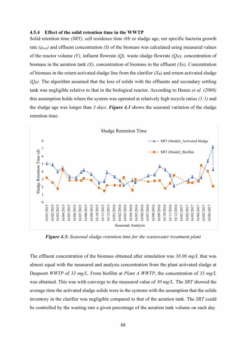
88

4.5.4 Effect of the solid retention time in the WWTP Solid retention time (SRT), cell residence time (Ɵ) or sludge age, net specific bacteria growth

rate (µnet) and effluent concentration (S) of the biomass was calculated using measured values

of the reactor volume (V), influent flowrate (Q), waste sludge flowrate (QW), concentration of

biomass in the aeration tank (X), concentration of biomass in the effluent (Xe), Concentration

of biomass in the return activated sludge line from the clarifier (XR) and return activated sludge

(QR). The algorithm assumed that the loss of solids with the effluents and secondary settling

tank was negligible relative to that in the biological reactor. According to Henze et al. (2008)

this assumption holds where the system was operated at relatively high recycle ratios (1:1) and

the sludge age was longer than 3 days. Figure 4.3 shows the seasonal variation of the sludge

retention time.

Figure 4.3: Seasonal sludge retention time for the wastewater treatment plant

The effluent concentration of the biomass obtained after simulation was 38.06 mg/L that was

almost equal with the measured and analysis concentration from the plant activated sludge at

Daspoort WWTP of 33 mg/L. From biofilm at Plant A WWTP, the concentration of 33 mg/L

was obtained. This was with converge to the measured value of 30 mg/L. The SRT showed the

average time the activated sludge solids were in the systems with the assumption that the solids

inventory in the clarifier was negligible compared to that of the aeration tank. The SRT could

be controlled by the wasting rate a given percentage of the aeration tank volume on each day.

0

1

2

3

4

5

6

7

8

16/0

1/20

1516

/02/

2015

16/0

3/20

1516

/04/

2015

16/0

5/20

1516

/06/

2015

16/0

7/20

1516

/08/

2015

16/0

9/20

1516

/10/

2015

16/1

1/20

1516

/12/

2015

16/0

1/20

1616

/02/

2016

16/0

3/20

1616

/04/

2016

16/0

5/20

1616

/06/

2016

16/0

7/20

1616

/08/

2016

16/0

9/20

1616

/10/

2016

16/1

1/20

1616

/12/

2016

16/0

1/20

1716

/02/

2017

16/0

3/20

1716

/04/

2017

16/0

5/20

1716

/06/

2017

Slud

ge R

eten

tion

Tim

e (d

)

Seasonal Analysis

Sludge Retention Time

SRT (Model)_Activated Sludge

SRT (Model)_Biofilm

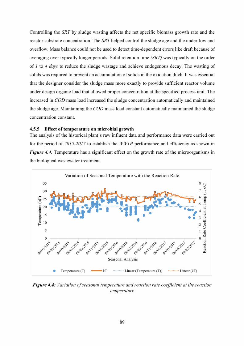
89

Controlling the SRT by sludge wasting affects the net specific biomass growth rate and the

reactor substrate concentration. The SRT helped control the sludge age and the underflow and

overflow. Mass balance could not be used to detect time-dependent errors like draft because of

averaging over typically longer periods. Solid retention time (SRT) was typically on the order

of 1 to 4 days to reduce the sludge wastage and achieve endogenous decay. The wasting of

solids was required to prevent an accumulation of solids in the oxidation ditch. It was essential

that the designer consider the sludge mass more exactly to provide sufficient reactor volume

under design organic load that allowed proper concentration at the specified process unit. The

increased in COD mass load increased the sludge concentration automatically and maintained

the sludge age. Maintaining the COD mass load constant automatically maintained the sludge

concentration constant.

4.5.5 Effect of temperature on microbial growth The analysis of the historical plant’s raw influent data and performance data were carried out

for the period of 2015-2017 to establish the WWTP performance and efficiency as shown in

Figure 4.4. Temperature has a significant effect on the growth rate of the microorganisms in

the biological wastewater treatment.

Figure 4.4: Variation of seasonal temperature and reaction rate coefficient at the reaction temperature

0

1

2

3

4

5

6

7

8

0

5

10

15

20

25

30

35

Rea

ctio

n R

ate

Coe

ffici

ent a

t Tem

p (T

, oC

)

Tem

pera

ture

(oC

)

Seasonal Analysis

Variation of Seasonal Temperature with the Reaction Rate

Temperature (T) kT Linear (Temperature (T)) Linear (kT)

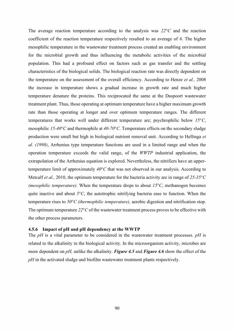
90

The average reaction temperature according to the analysis was 22°C and the reaction

coefficient of the reaction temperature respectively resulted to an average of 6. The higher

mesophilic temperature in the wastewater treatment process created an enabling environment

for the microbial growth and thus influencing the metabolic activities of the microbial

population. This had a profound effect on factors such as gas transfer and the settling

characteristics of the biological solids. The biological reaction rate was directly dependent on

the temperature on the assessment of the overall efficiency. According to Henze et al., 2008

the increase in temperature shows a gradual increase in growth rate and much higher

temperature denature the proteins. This reciprocated the same at the Daspoort wastewater

treatment plant. Thus, those operating at optimum temperature have a higher maximum growth

rate than those operating at longer and over optimum temperature ranges. The different

temperatures that works well under different temperature are; psychrophilic below 15°C,

mesophilic 15-40°C and thermophile at 40-70°C. Temperature effects on the secondary sludge

production were small but high in biological nutrient removal unit. According to Hellinga et

al. (1998), Arrhenius type temperature functions are used in a limited range and when the

operation temperature exceeds the valid range, of the WWTP industrial application, the

extrapolation of the Arrhenius equation is explored. Nevertheless, the nitrifiers have an upper-

temperature limit of approximately 40°C that was not observed in our analysis. According to

Metcalf et al., 2010, the optimum temperature for the bacteria activity are in range of 25-35°C

(mesophilic temperature). When the temperature drops to about 15°C, methanogen becomes

quite inactive and about 5°C, the autotrophic nitrifying bacteria ease to function. When the

temperature rises to 50°C (thermophilic temperature), aerobic digestion and nitrification stop.

The optimum temperature 22°C of the wastewater treatment process proves to be effective with

the other process parameters.

4.5.6 Impact of pH and pH dependency at the WWTP The pH is a vital parameter to be considered in the wastewater treatment processes. pH is

related to the alkalinity in the biological activity. In the microorganism activity, microbes are

more dependent on pH, unlike the alkalinity. Figure 4.5 and Figure 4.6 show the effect of the

pH in the activated sludge and biofilm wastewater treatment plants respectively.

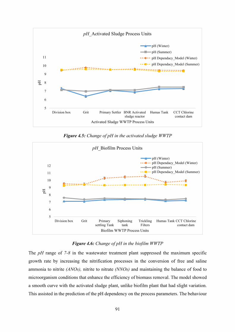
91

Figure 4.5: Change of pH in the activated sludge WWTP

Figure 4.6: Change of pH in the biofilm WWTP

The pH range of 7-8 in the wastewater treatment plant suppressed the maximum specific

growth rate by increasing the nitrification processes in the conversion of free and saline

ammonia to nitrite (ANOs), nitrite to nitrate (NNOs) and maintaining the balance of food to

microorganism conditions that enhance the efficiency of biomass removal. The model showed

a smooth curve with the activated sludge plant, unlike biofilm plant that had slight variation.

This assisted in the prediction of the pH dependency on the process parameters. The behaviour

5

6

7

8

9

10

11

Division box Grit Primary Settler BNR Activatedsludge reactor

Humas Tank CCT Chlorinecontact dam

pH

Activated Sludge WWTP Process Units

pH_Activated Sludge Process Units

pH (Winter)

pH (Summer)

pH Dependacy_Model (Winter)

pH Dependacy_Model (Summer)

5

6

7

8

9

10

11

12

Division box Grit Primarysettling Tank

Siphoningtank

TricklingFilters


pH

Biofilm WWTP Process Units

pH_Biofilm Process Units

pH (Winter)pH Dependacy_Model (Winter)pH (Summer)pH Dependacy_Model (Summer)

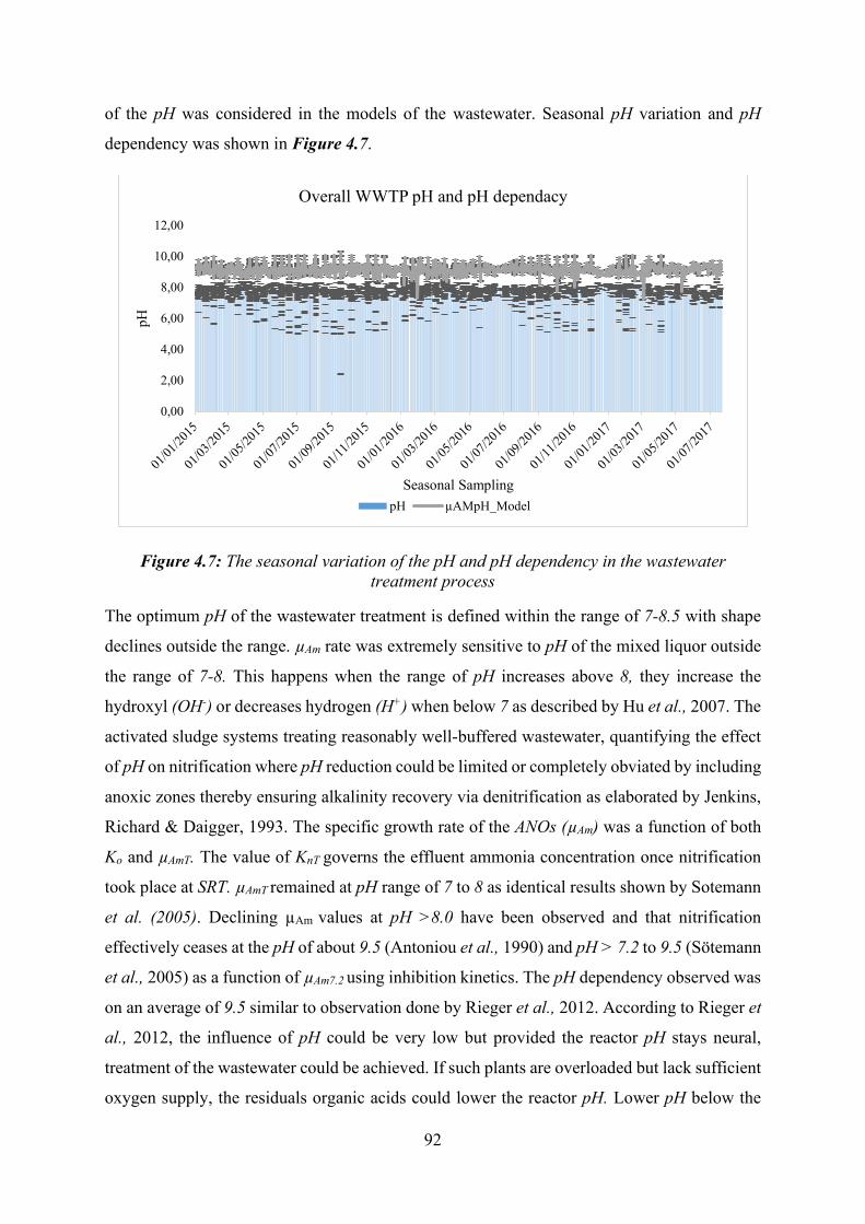
92

of the pH was considered in the models of the wastewater. Seasonal pH variation and pH

dependency was shown in Figure 4.7.

Figure 4.7: The seasonal variation of the pH and pH dependency in the wastewater treatment process

The optimum pH of the wastewater treatment is defined within the range of 7-8.5 with shape

declines outside the range. µAm rate was extremely sensitive to pH of the mixed liquor outside

the range of 7-8. This happens when the range of pH increases above 8, they increase the

hydroxyl (OH-) or decreases hydrogen (H+) when below 7 as described by Hu et al., 2007. The

activated sludge systems treating reasonably well-buffered wastewater, quantifying the effect

of pH on nitrification where pH reduction could be limited or completely obviated by including

anoxic zones thereby ensuring alkalinity recovery via denitrification as elaborated by Jenkins,

Richard & Daigger, 1993. The specific growth rate of the ANOs (µAm) was a function of both

Ko and µAmT. The value of KnT governs the effluent ammonia concentration once nitrification

took place at SRT. µAmT remained at pH range of 7 to 8 as identical results shown by Sotemann

et al. (2005). Declining µAm values at pH >8.0 have been observed and that nitrification

effectively ceases at the pH of about 9.5 (Antoniou et al., 1990) and pH > 7.2 to 9.5 (Sötemann

et al., 2005) as a function of µAm7.2 using inhibition kinetics. The pH dependency observed was

on an average of 9.5 similar to observation done by Rieger et al., 2012. According to Rieger et

al., 2012, the influence of pH could be very low but provided the reactor pH stays neural,

treatment of the wastewater could be achieved. If such plants are overloaded but lack sufficient

oxygen supply, the residuals organic acids could lower the reactor pH. Lower pH below the

0,00

2,00

4,00

6,00

8,00

10,00

12,00

pH

Seasonal Sampling

Overall WWTP pH and pH dependacy

pH µAMpH_Model

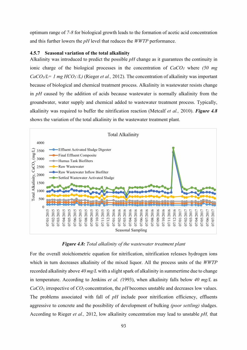
93

optimum range of 7-8 for biological growth leads to the formation of acetic acid concentration

and this further lowers the pH level that reduces the WWTP performance.

4.5.7 Seasonal variation of the total alkalinity Alkalinity was introduced to predict the possible pH change as it guarantees the continuity in

ionic charge of the biological processes in the concentration of CaCO3, where (50 mg

CaCO3/L= 1 mg HCO3-/L) (Rieger et al., 2012). The concentration of alkalinity was important

because of biological and chemical treatment process. Alkalinity in wastewater resists change

in pH caused by the addition of acids because wastewater is normally alkalinity from the

groundwater, water supply and chemical added to wastewater treatment process. Typically,

alkalinity was required to buffer the nitrification reaction (Metcalf et al., 2010). Figure 4.8

shows the variation of the total alkalinity in the wastewater treatment plant.

Figure 4.8: Total alkalinity of the wastewater treatment plant

For the overall stoichiometric equation for nitrification, nitrification releases hydrogen ions

which in turn decreases alkalinity of the mixed liquor. All the process units of the WWTP

recorded alkalinity above 40 mg/L with a slight spark of alkalinity in summertime due to change

in temperature. According to Jenkins et al. (1993), when alkalinity falls below 40 mg/L as

CaCO3, irrespective of CO2 concentration, the pH becomes unstable and decreases low values.

The problems associated with fall of pH include poor nitrification efficiency, effluents

aggressive to concrete and the possibility of development of bulking (poor settling) sludges.

According to Rieger et al., 2012, low alkalinity concentration may lead to unstable pH, that

0

500

1000

1500

2000

2500

3000

3500

4000

07/0

1/20

1507

/02/

2015

07/0

3/20

1507

/04/

2015

07/0

5/20

1507

/06/

2015

07/0

7/20

1507

/08/

2015

07/0

9/20

1507

/10/

2015

07/1

1/20

1507

/12/

2015

07/0

1/20

1607

/02/

2016

07/0

3/20

1607

/04/

2016

07/0

5/20

1607

/06/

2016

07/0

7/20

1607

/08/

2016

07/0

9/20

1607

/10/

2016

07/1

1/20

1607

/12/

2016

07/0

1/20

1707

/02/

2017

07/0

3/20

1707

/04/

2017

07/0

5/20

1707

/06/

2017

07/0

7/20

17

Tota

l Alk

alin

ity, C

aCO

3(m

g/L)

Seasonal Sampling

Total Alkalinity

Effluent Activated Sludge DigesterFinal Effluent CompositeHumus Tank BiofiltersRaw WastewaterRaw Wastewater Inflow BiofilterSettled Wastewater Activated Sludge

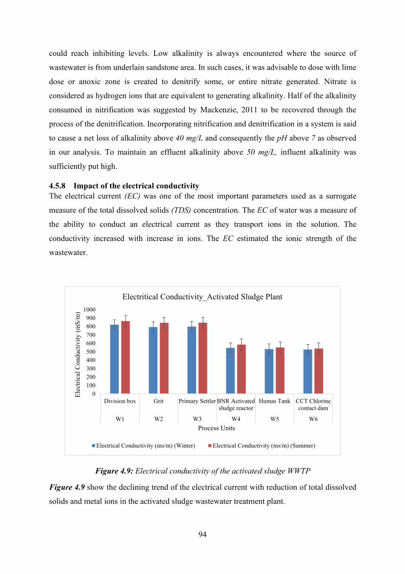
94

could reach inhibiting levels. Low alkalinity is always encountered where the source of

wastewater is from underlain sandstone area. In such cases, it was advisable to dose with lime

dose or anoxic zone is created to denitrify some, or entire nitrate generated. Nitrate is

considered as hydrogen ions that are equivalent to generating alkalinity. Half of the alkalinity

consumed in nitrification was suggested by Mackenzie, 2011 to be recovered through the

process of the denitrification. Incorporating nitrification and denitrification in a system is said

to cause a net loss of alkalinity above 40 mg/L and consequently the pH above 7 as observed

in our analysis. To maintain an effluent alkalinity above 50 mg/L, influent alkalinity was

sufficiently put high.

4.5.8 Impact of the electrical conductivity The electrical current (EC) was one of the most important parameters used as a surrogate

measure of the total dissolved solids (TDS) concentration. The EC of water was a measure of

the ability to conduct an electrical current as they transport ions in the solution. The

conductivity increased with increase in ions. The EC estimated the ionic strength of the

wastewater.

Figure 4.9: Electrical conductivity of the activated sludge WWTP

Figure 4.9 show the declining trend of the electrical current with reduction of total dissolved

solids and metal ions in the activated sludge wastewater treatment plant.

0100200300400500600700800900

1000



W1 W2 W3 W4 W5 W6

Elec

trica

l Con

duct

ivity

(mS/

m)

Process Units

Electritical Conductivity_Activated Sludge Plant

Electrical Conductivity (ms/m) (Winter) Electrical Conductivity (ms/m) (Summer)

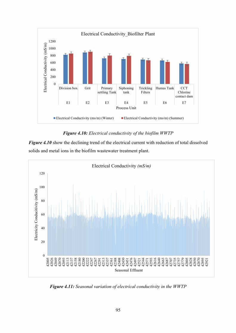
95

Figure 4.10: Electrical conductivity of the biofilm WWTP

Figure 4.10 show the declining trend of the electrical current with reduction of total dissolved

solids and metal ions in the biofilm wastewater treatment plant.

Figure 4.11: Seasonal variation of electrical conductivity in the WWTP

0

200

400

600

800

1000

1200


Siphoningtank

TricklingFilters

Humas Tank CCTChlorine

contact dam

E1 E2 E3 E4 E5 E6 E7

Elec

trica

l Con

duct

ivity

(mS/

m)

Process Unit

Electrical Conductivity_Biofilter Plant

Electrical Conductivity (ms/m) (Winter) Electrical Conductivity (ms/m) (Summer)

0

20

40

60

80

100

120

4200

542

026

4204

942

070

4209

342

113

4213

742

158

4218

042

200

4222

242

247

4226

742

291

4231

342

337

4236

142

388

4240

842

430

4245

142

476

4249

742

521

4254

442

571

4259

342

616

4264

042

663

4268

742

707

4273

542

757

4277

942

805

4282

842

850

4287

042

895

4292

1

Elec

trici

ty C

ondu

citiv

ity (m

S/m

)

Seasonal Effluent

Electrical Conductivity (mS/m)

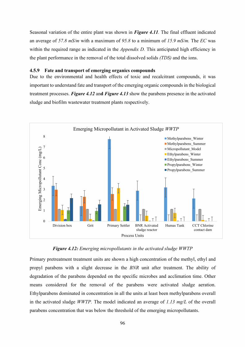
96

Seasonal variation of the entire plant was shown in Figure 4.11. The final effluent indicated

an average of 57.8 mS/m with a maximum of 95.8 to a minimum of 15.9 mS/m. The EC was

within the required range as indicated in the Appendix D. This anticipated high efficiency in

the plant performance in the removal of the total dissolved solids (TDS) and the ions.

4.5.9 Fate and transport of emerging organics compounds Due to the environmental and health effects of toxic and recalcitrant compounds, it was

important to understand fate and transport of the emerging organic compounds in the biological

treatment processes. Figure 4.12 and Figure 4.13 show the parabens presence in the activated

sludge and biofilm wastewater treatment plants respectively.

Figure 4.12: Emerging micropollutants in the activated sludge WWTP

Primary pretreatment treatment units are shown a high concentration of the methyl, ethyl and

propyl parabens with a slight decrease in the BNR unit after treatment. The ability of

degradation of the parabens depended on the specific microbes and acclimation time. Other

means considered for the removal of the parabens were activated sludge aeration.

Ethylparabens dominated in concentration in all the units at least been methylparabens overall

in the activated sludge WWTP. The model indicated an average of 1.13 mg/L of the overall

parabens concentration that was below the threshold of the emerging micropollutants.

0

1

2

3

4

5

6

7

8



Emer

ging

Mic

ropo

lluta

nt C

onc

(mg/

L)

Process Units

Emerging Micropollutant in Activated Sludge WWTP

Methylparabens_WinterMethylparabens_SummerMicropollutant_ModelEthylparabens_WinterEthylparabens_SummerPropylparabens_WinterPropylparabens_Summer

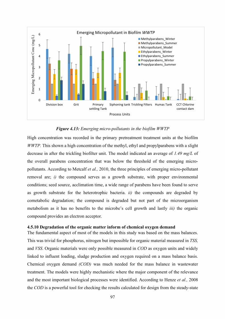
97

Figure 4.13: Emerging micro-pollutants in the biofilm WWTP

High concentration was recorded in the primary pretreatment treatment units at the biofilm

WWTP. This shown a high concentration of the methyl, ethyl and propylparabens with a slight

decrease in after the trickling biofilter unit. The model indicated an average of 1.49 mg/L of

the overall parabens concentration that was below the threshold of the emerging micro-

pollutants. According to Metcalf et al., 2010, the three principles of emerging micro-pollutant

removal are; i) the compound serves as a growth substrate, with proper environmental

conditions; seed source, acclimation time, a wide range of parabens have been found to serve

as growth substrate for the heterotrophic bacteria. ii) the compounds are degraded by

cometabolic degradation; the compound is degraded but not part of the microorganism

metabolism as it has no benefits to the microbe’s cell growth and lastly iii) the organic

compound provides an electron acceptor.

4.5.10 Degradation of the organic matter inform of chemical oxygen demand The fundamental aspect of most of the models in this study was based on the mass balances.

This was trivial for phosphorus, nitrogen but impossible for organic material measured in TSS,

and VSS. Organic materials were only possible measured in COD as oxygen units and widely

linked to influent loading, sludge production and oxygen required on a mass balance basis.

Chemical oxygen demand (COD) was much needed for the mass balance in wastewater

treatment. The models were highly mechanistic where the major component of the relevance

and the most important biological processes were identified. According to Henze et al., 2008

the COD is a powerful tool for checking the results calculated for design from the steady-state

0

1

2

3

4

5

6


Siphoning tank Trickling Filters Humas Tank CCT Chlorinecontact dam

Emer

ging

Mic

ropo

lluta

nt C

onc

(mg/

L)

Process Units

Emerging Micropollutant in Biofilm WWTPMethylparabens_WinterMethylparabens_SummerMicropollutant_ModelEthylparabens_WinterEthylparabens_SummerPropylparabens_WinterPropylparabens_Summer

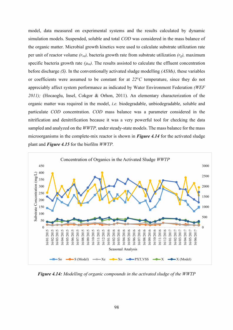
98

model, data measured on experimental systems and the results calculated by dynamic

simulation models. Suspended, soluble and total COD was considered in the mass balance of

the organic matter. Microbial growth kinetics were used to calculate substrate utilization rate

per unit of reactor volume (rsu), bacteria growth rate from substrate utilization (rg), maximum

specific bacteria growth rate (µm). The results assisted to calculate the effluent concentration

before discharge (S). In the conventionally activated sludge modelling (ASMs), these variables

or coefficients were assumed to be constant for at 22°C temperature, since they do not

appreciably affect system performance as indicated by Water Environment Federation (WEF

2011); (Hocaoglu, Insel, Cokgor & Orhon, 2011). An elementary characterization of the

organic matter was required in the model, i.e. biodegradable, unbiodegradable, soluble and

particulate COD concentration. COD mass balance was a parameter considered in the

nitrification and denitrification because it was a very powerful tool for checking the data

sampled and analyzed on the WWTP, under steady-state models. The mass balance for the mass

microorganisms in the complete-mix reactor is shown in Figure 4.14 for the activated sludge

plant and Figure 4.15 for the biofilm WWTP.

Figure 4.14: Modelling of organic compounds in the activated sludge of the WWTP

0

500

1000

1500

2000

2500

3000

0

50

100

150

200

250

300

350

400

450

16/0

1/20

1516

/02/

2015

16/0

3/20

1516

/04/

2015

16/0

5/20

1516

/06/

2015

16/0

7/20

1516

/08/

2015

16/0

9/20

1516

/10/

2015

16/1

1/20

1516

/12/

2015

16/0

1/20

1616

/02/

2016

16/0

3/20

1616

/04/

2016

16/0

5/20

1616

/06/

2016

16/0

7/20

1616

/08/

2016

16/0

9/20

1616

/10/

2016

16/1

1/20

1616

/12/

2016

16/0

1/20

1716

/02/

2017

16/0

3/20

1716

/04/

2017

16/0

5/20

1716

/06/

2017

Subs

trate

Con

cent

ratio

n (m

g/L)

Seasonal Analysis

Concentration of Organics in the Activated Sludge WWTP

So S (Model) Xe Xo PXT,VSS X X (Model)

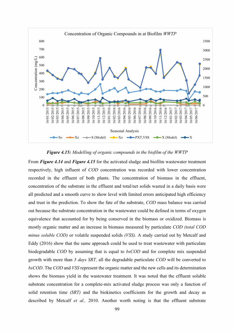
99

Figure 4.15: Modelling of organic compounds in the biofilm of the WWTP

From Figure 4.14 and Figure 4.15 for the activated sludge and biofilm wastewater treatment

respectively, high influent of COD concentration was recorded with lower concentration

recorded in the effluent of both plants. The concentration of biomass in the effluent,

concentration of the substrate in the effluent and total/net solids wasted in a daily basis were

all predicted and a smooth curve to show level with limited errors anticipated high efficiency

and trust in the prediction. To show the fate of the substrate, COD mass balance was carried

out because the substrate concentration in the wastewater could be defined in terms of oxygen

equivalence that accounted for by being conserved in the biomass or oxidized. Biomass is

mostly organic matter and an increase in biomass measured by particulate COD (total COD

minus soluble COD) or volatile suspended solids (VSS). A study carried out by Metcalf and

Eddy (2016) show that the same approach could be used to treat wastewater with particulate

biodegradable COD by assuming that is equal to bsCOD and for complete mix suspended

growth with more than 3 days SRT, all the degradable particulate COD will be converted to

bsCOD. The COD and VSS represent the organic matter and the new cells and its determination

shows the biomass yield in the wastewater treatment. It was noted that the effluent soluble

substrate concentration for a complete-mix activated sludge process was only a function of

solid retention time (SRT) and the biokinetics coefficients for the growth and decay as

described by Metcalf et al., 2010. Another worth noting is that the effluent substrate

0

500

1000

1500

2000

2500

3000

3500

0

100

200

300

400

500

600

700

80016

/01/

2015

16/0

2/20

1516

/03/

2015

16/0

4/20

1516

/05/

2015

16/0

6/20

1516

/07/

2015

16/0

8/20

1516

/09/

2015

16/1

0/20

1516

/11/

2015

16/1

2/20

1516

/01/

2016

16/0

2/20

1616

/03/

2016

16/0

4/20

1616

/05/

2016

16/0

6/20

1616

/07/

2016

16/0

8/20

1616

/09/

2016

16/1

0/20

1616

/11/

2016

16/1

2/20

1616

/01/

2017

16/0

2/20

1716

/03/

2017

16/0

4/20

1716

/05/

2017

16/0

6/20

17

Con

cent

ratio

n (m

g/L)

Seasonal Analysis

Concentration of Organic Compounds in at Biofilm WWTP

So Xe S (Model) Xo PXT,VSS X (Model) X

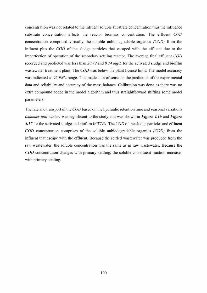
100

concentration was not related to the influent soluble substrate concentration thus the influence

substrate concentration affects the reactor biomass concentration. The effluent COD

concentration comprised virtually the soluble unbiodegradable organics (COD) from the

influent plus the COD of the sludge particles that escaped with the effluent due to the

imperfection of operation of the secondary settling reactor. The average final effluent COD

recorded and predicted was less than 20.72 and 0.74 mg/L for the activated sludge and biofilm

wastewater treatment plant. The COD was below the plant license limit. The model accuracy

was indicated as 95-98% range. That made a lot of sense on the prediction of the experimental

data and reliability and accuracy of the mass balance. Calibration was done as there was no

extra compound added in the model algorithm and thus straightforward shifting some model

parameters.

The fate and transport of the COD based on the hydraulic retention time and seasonal variations

(summer and winter) was significant to the study and was shown in Figure 4.16 and Figure

4.17 for the activated sludge and biofilm WWTPs. The COD of the sludge particles and effluent

COD concentration comprises of the soluble unbiodegradable organics (COD) from the

influent that escape with the effluent. Because the settled wastewater was produced from the

raw wastewater, the soluble concentration was the same as in raw wastewater. Because the

COD concentration changes with primary settling, the soluble constituent fraction increases

with primary settling.

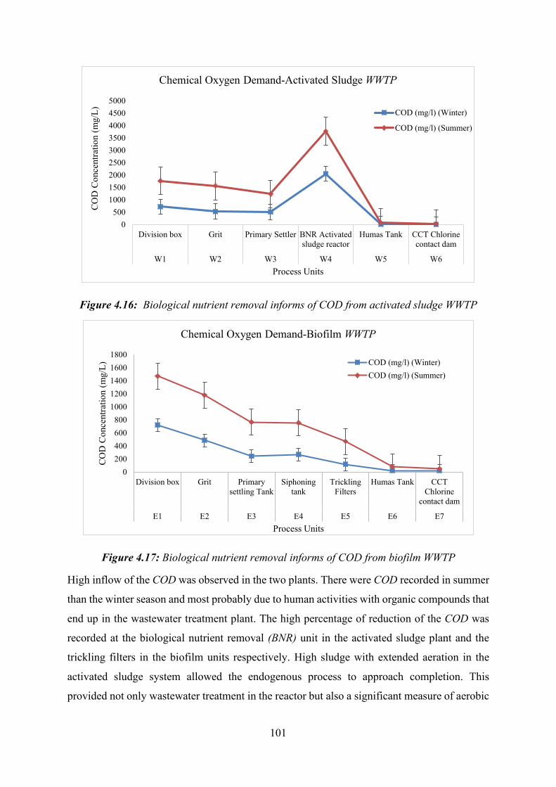
101

Figure 4.16: Biological nutrient removal informs of COD from activated sludge WWTP

Figure 4.17: Biological nutrient removal informs of COD from biofilm WWTP

High inflow of the COD was observed in the two plants. There were COD recorded in summer

than the winter season and most probably due to human activities with organic compounds that

end up in the wastewater treatment plant. The high percentage of reduction of the COD was

recorded at the biological nutrient removal (BNR) unit in the activated sludge plant and the

trickling filters in the biofilm units respectively. High sludge with extended aeration in the

activated sludge system allowed the endogenous process to approach completion. This

provided not only wastewater treatment in the reactor but also a significant measure of aerobic

0500

100015002000250030003500400045005000



W1 W2 W3 W4 W5 W6

CO

D C

once

ntra

tion

(mg/

L)

Process Units

Chemical Oxygen Demand-Activated Sludge WWTP

COD (mg/l) (Winter)

COD (mg/l) (Summer)

0200400600800

10001200140016001800


Siphoningtank

TricklingFilters

Humas Tank CCTChlorine

contact dam

E1 E2 E3 E4 E5 E6 E7

CO

D C

once

ntra

tion

(mg/

L)

Process Units

Chemical Oxygen Demand-Biofilm WWTP

COD (mg/l) (Winter)COD (mg/l) (Summer)

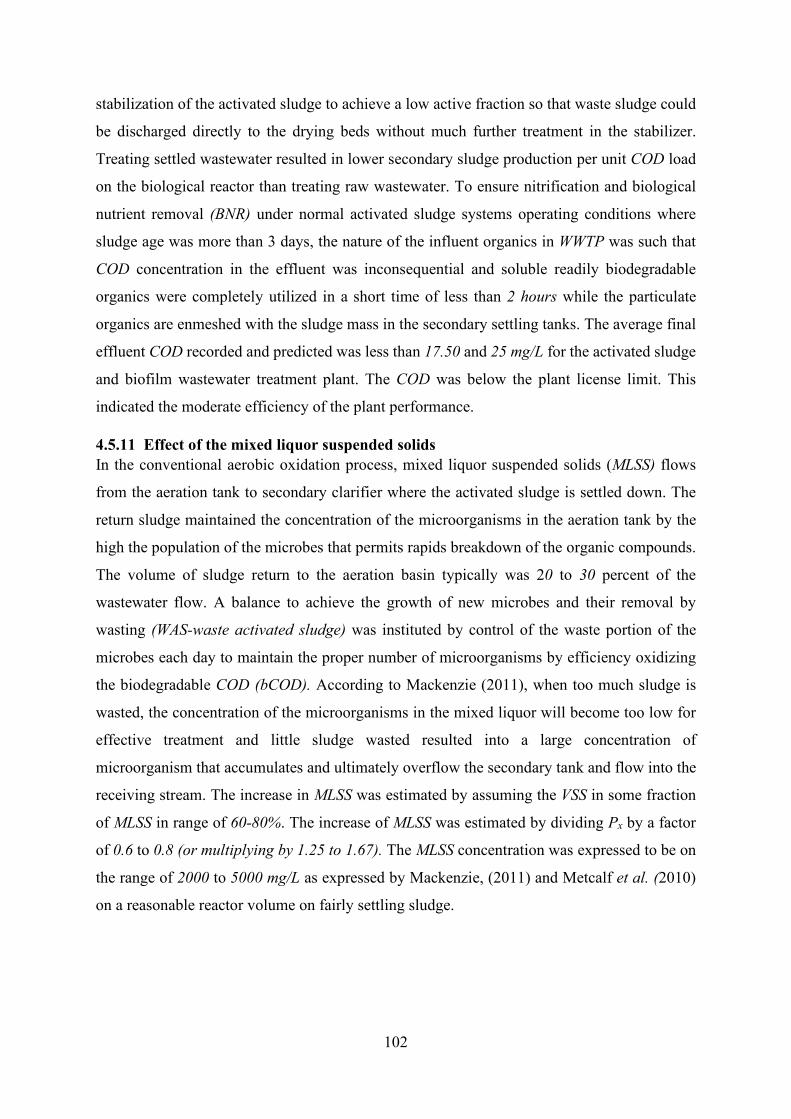
102

stabilization of the activated sludge to achieve a low active fraction so that waste sludge could

be discharged directly to the drying beds without much further treatment in the stabilizer.

Treating settled wastewater resulted in lower secondary sludge production per unit COD load

on the biological reactor than treating raw wastewater. To ensure nitrification and biological

nutrient removal (BNR) under normal activated sludge systems operating conditions where

sludge age was more than 3 days, the nature of the influent organics in WWTP was such that

COD concentration in the effluent was inconsequential and soluble readily biodegradable

organics were completely utilized in a short time of less than 2 hours while the particulate

organics are enmeshed with the sludge mass in the secondary settling tanks. The average final

effluent COD recorded and predicted was less than 17.50 and 25 mg/L for the activated sludge

and biofilm wastewater treatment plant. The COD was below the plant license limit. This

indicated the moderate efficiency of the plant performance.

4.5.11 Effect of the mixed liquor suspended solids In the conventional aerobic oxidation process, mixed liquor suspended solids (MLSS) flows

from the aeration tank to secondary clarifier where the activated sludge is settled down. The

return sludge maintained the concentration of the microorganisms in the aeration tank by the

high the population of the microbes that permits rapids breakdown of the organic compounds.

The volume of sludge return to the aeration basin typically was 20 to 30 percent of the

wastewater flow. A balance to achieve the growth of new microbes and their removal by

wasting (WAS-waste activated sludge) was instituted by control of the waste portion of the

microbes each day to maintain the proper number of microorganisms by efficiency oxidizing

the biodegradable COD (bCOD). According to Mackenzie (2011), when too much sludge is

wasted, the concentration of the microorganisms in the mixed liquor will become too low for

effective treatment and little sludge wasted resulted into a large concentration of

microorganism that accumulates and ultimately overflow the secondary tank and flow into the

receiving stream. The increase in MLSS was estimated by assuming the VSS in some fraction

of MLSS in range of 60-80%. The increase of MLSS was estimated by dividing Px by a factor

of 0.6 to 0.8 (or multiplying by 1.25 to 1.67). The MLSS concentration was expressed to be on

the range of 2000 to 5000 mg/L as expressed by Mackenzie, (2011) and Metcalf et al. (2010)

on a reasonable reactor volume on fairly settling sludge.

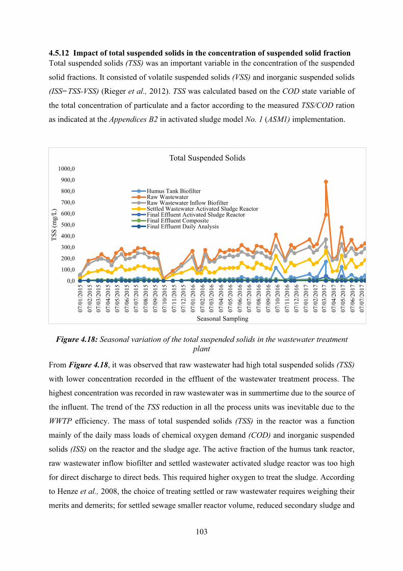
103

4.5.12 Impact of total suspended solids in the concentration of suspended solid fraction Total suspended solids (TSS) was an important variable in the concentration of the suspended

solid fractions. It consisted of volatile suspended solids (VSS) and inorganic suspended solids

(ISS=TSS-VSS) (Rieger et al., 2012). TSS was calculated based on the COD state variable of

the total concentration of particulate and a factor according to the measured TSS/COD ration

as indicated at the Appendices B2 in activated sludge model No. 1 (ASM1) implementation.

Figure 4.18: Seasonal variation of the total suspended solids in the wastewater treatment plant

From Figure 4.18, it was observed that raw wastewater had high total suspended solids (TSS)

with lower concentration recorded in the effluent of the wastewater treatment process. The

highest concentration was recorded in raw wastewater was in summertime due to the source of

the influent. The trend of the TSS reduction in all the process units was inevitable due to the

WWTP efficiency. The mass of total suspended solids (TSS) in the reactor was a function

mainly of the daily mass loads of chemical oxygen demand (COD) and inorganic suspended

solids (ISS) on the reactor and the sludge age. The active fraction of the humus tank reactor,

raw wastewater inflow biofilter and settled wastewater activated sludge reactor was too high

for direct discharge to direct beds. This required higher oxygen to treat the sludge. According

to Henze et al., 2008, the choice of treating settled or raw wastewater requires weighing their

merits and demerits; for settled sewage smaller reactor volume, reduced secondary sludge and

0,0

100,0

200,0

300,0

400,0

500,0

600,0

700,0

800,0

900,0

1000,0

07/0

1/20

1507

/02/

2015

07/0

3/20

1507

/04/

2015

07/0

5/20

1507

/06/

2015

07/0

7/20

1507

/08/

2015

07/0

9/20

1507

/10/

2015

07/1

1/20

1507

/12/

2015

07/0

1/20

1607

/02/

2016

07/0

3/20

1607

/04/

2016

07/0

5/20

1607

/06/

2016

07/0

7/20

1607

/08/

2016

07/0

9/20

1607

/10/

2016

07/1

1/20

1607

/12/

2016

07/0

1/20

1707

/02/

2017

07/0

3/20

1707

/04/

2017

07/0

5/20

1707

/06/

2017

07/0

7/20

17

TSS

(mg/

L)

Seasonal Sampling

Total Suspended Solids

Humus Tank BiofilterRaw WastewaterRaw Wastewater Inflow BiofilterSettled Wastewater Activated Sludge ReactorFinal Effluent Activated Sludge ReactorFinal Effluent CompositeFinal Effluent Daily Analysis

104

lower oxygen demand, but deals with secondary and primary sludge and their stabilization but

for raw sewage and larger reactor volume, higher oxygen demand and increased secondary

sludge production, but having no primary sludge to deal with. The TSS concentration difference

from the settled, raw wastewater arises because the sludge settle ability in conventional systems

could be poorer than extended aeration system and the wastewater flow per kg COD loaded on

the reactor for raw wastewater was significantly greater than that for settled wastewater. TSS

was used to assess the performance of the conventional treatment process and the need for

effluent filtration in reuse application. It was one of the universal used effluent standards by

which the performance of treatment plants was judged for the regulatory control purposes.

4.5.13 Variation of the volatile suspended solids in WWTP The mass of volatile suspended solids (VSS) in the reactor was a function of the daily COD

mass load on it and the sludge age. Figure 4.19 presents the seasonal variation of the VSS in

the wastewater treatment plant.

Figure 4.19: Seasonal variation of the volatile suspended solids-mixed mixed liquor of the WWTP.

A higher VSS of 5145 mg/L was recorded on the summer time with lower VSS of 64 mg/L

recorded in summer period again. This showed inconsistency in the efficiency with volatile

suspended solids in the plant’s operation and most probably the source of the influent defined

the source of the TSS in the plant. The average VSS was indicated as 1356.97 mg/L that was in

compliance with the wastewater treatment license (Appendix D).

0

1000

2000

3000

4000

5000

6000

04/0

2/20

1504

/03/

2015

04/0

4/20

1504

/05/

2015

04/0

6/20

1504

/07/

2015

04/0

8/20

1504

/09/

2015

04/1

0/20

1504

/11/

2015

04/1

2/20

1504

/01/

2016

04/0

2/20

1604

/03/

2016

04/0

4/20

1604

/05/

2016

04/0

6/20

1604

/07/

2016

04/0

8/20

1604

/09/

2016

04/1

0/20

1604

/11/

2016

04/1

2/20

1604

/01/

2017

04/0

2/20

1704

/03/

2017

04/0

4/20

1704

/05/

2017

04/0

6/20

1704

/07/

2017

VSS

(MG

/L)

Seasonal Analysis

Volatile Suspended Solids

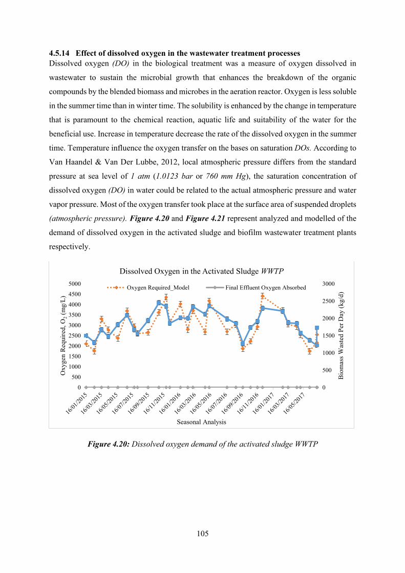
105

4.5.14 Effect of dissolved oxygen in the wastewater treatment processes Dissolved oxygen (DO) in the biological treatment was a measure of oxygen dissolved in

wastewater to sustain the microbial growth that enhances the breakdown of the organic

compounds by the blended biomass and microbes in the aeration reactor. Oxygen is less soluble

in the summer time than in winter time. The solubility is enhanced by the change in temperature

that is paramount to the chemical reaction, aquatic life and suitability of the water for the

beneficial use. Increase in temperature decrease the rate of the dissolved oxygen in the summer

time. Temperature influence the oxygen transfer on the bases on saturation DOs. According to

Van Haandel & Van Der Lubbe, 2012, local atmospheric pressure differs from the standard

pressure at sea level of 1 atm (1.0123 bar or 760 mm Hg), the saturation concentration of

dissolved oxygen (DO) in water could be related to the actual atmospheric pressure and water

vapor pressure. Most of the oxygen transfer took place at the surface area of suspended droplets

(atmospheric pressure). Figure 4.20 and Figure 4.21 represent analyzed and modelled of the

demand of dissolved oxygen in the activated sludge and biofilm wastewater treatment plants

respectively.

Figure 4.20: Dissolved oxygen demand of the activated sludge WWTP

0

500

1000

1500

2000

2500

3000

0

500

1000

1500

2000

2500

3000

3500

4000

4500

5000

Bio

mas

s W

aste

d Pe

r Day

(kg/

d)

Oxy

gen

Req

uire

d, O

2(m

g/L)

Seasonal Analysis

Dissolved Oxygen in the Activated Sludge WWTP

Oxygen Required_Model Final Effluent Oxygen Absorbed

106

Figure 4.21: Dissolved oxygen demand of the biofilm WWTP

The activated sludge plant showed the smooth curve of the model and analyzed DO, unlike the

biofilm where there were small errors in the variation due to lack of recycled stream to circulate

the oxygen like the MLSS in the aeration reactor. For the COD balance, the more oxygen that

is utilized in the system, the lower the sludge production and the lower the active fraction of

the sludge observed. An adequate supply of dissolved oxygen enhanced nitrification. Our

findings recorded high oxygen requirement from the model of a maximum of 596.70 mg/L and

minimum of 307.16 mg/L in the biofilm WWTP. Higher DO required was recorded in the

activated sludge due to plant capacity with the 4355.5 mg/L and minimum of 1759.5mg/L. At

DO value below Ko, the growth rate declined to less than half the rate where oxygen was present

in adequate concentration. High range of Ko risen when the concentration of DO was not same

as biological floc where the oxygen consumption took place. The DO level acted as the main

diffusion control parameter regulating the extent of simultaneous nitrification and

denitrification with different MLSS levels. The variation of DO depend on mixing intensity,

sludge settling properties floc size, microbial community, reactor volume due to discrete points

of oxygen input (mechanical aeration), and oxygen diffusion rate into the floc. The factors that

affect oxygen diffusion in flocs among others included the variation between measured results

due to steady-state and dynamic measuring techniques. According to Guo et al., 2009, lower

DO produces sludge with power settling properties but attain lower turbidities of the effluent

that high DO. DO deficiency was believed to be one of the most frequent causes responsible

for the most filamentous bacteria proliferation in activated sludge processes. The final effluent

0

500

1000

1500

2000

2500

3000

3500

0

100

200

300

400

500

600

700

Bio

mas

s W

aste

d pe

r day

(kg/

d)

Oxy

gen

Req

uire

d, O

2(m

g/L)

Seasonal Analysis

Dissolved Oxygen in the Biofilter WWTP

Oxygen Required_Model Final Effluent Oxygen Absorbed

107

oxygen absorbed recorded was 3.3 mg/L for the both activated sludge and biofilm WWTP.

According to Stenstrom & Poduska (1980), the maximum growth rate of both nitrification

reaction to be affected by dissolved oxygen concentration was in excess of 0.4 mg/L while

others have found that the most reliable range of DO concentration in nitrification to be

achieved as 0.5-2 mg/L. Another study by Henze et al., 2008 state that high dissolved oxygen

concentration up to 33 mg O2/L do not appear to affect the nitrification rates. However, low

oxygen concentration reduces the nitrification rates. Energy saving by low DO will be feasible

if sludge settleability did not become weak to affect the separation of sludge and effluent. It

was advisable for nitrification to proceed without inhibition by oxygen limitation though

adequately designed aeration equipment to supply the total oxygen demand. The DO above 2

mg/L allowed nitrification to proceed with efficiency because the surface aerators, adequate

velocity and aerator spacing were well fixed.

4.5.15 Sequence in the biological nitrogen removal

4.5.15.1 Nitrite and nitrate in form of N

All the biological materials and some unbiodegradable organic compounds contain nitrogen

(N). Biological nitrogen removal (BNR), (nitrification-denitrification-NDN or BNDN) requires

both anoxic and aerobic zone (Mackenzie, 2011; WEF, 2006). The volatile suspended solids

(VSS) that accumulate in the biological reactor comprises unbiodegradable particulate organics

(X1), active organisms (XBH), and endogenous residue (XEH). Nitrogen removal was assesses

based on monthly average data with the target effluent limit of 10 mg/L total nitrogen using a

steady state model.

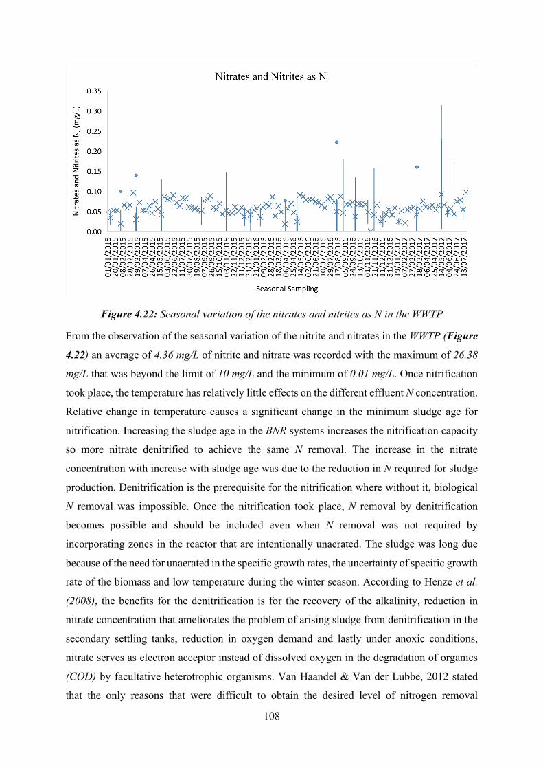
108

Figure 4.22: Seasonal variation of the nitrates and nitrites as N in the WWTP

From the observation of the seasonal variation of the nitrite and nitrates in the WWTP (Figure

4.22) an average of 4.36 mg/L of nitrite and nitrate was recorded with the maximum of 26.38

mg/L that was beyond the limit of 10 mg/L and the minimum of 0.01 mg/L. Once nitrification

took place, the temperature has relatively little effects on the different effluent N concentration.

Relative change in temperature causes a significant change in the minimum sludge age for

nitrification. Increasing the sludge age in the BNR systems increases the nitrification capacity

so more nitrate denitrified to achieve the same N removal. The increase in the nitrate

concentration with increase with sludge age was due to the reduction in N required for sludge

production. Denitrification is the prerequisite for the nitrification where without it, biological

N removal was impossible. Once the nitrification took place, N removal by denitrification

becomes possible and should be included even when N removal was not required by

incorporating zones in the reactor that are intentionally unaerated. The sludge was long due

because of the need for unaerated in the specific growth rates, the uncertainty of specific growth

rate of the biomass and low temperature during the winter season. According to Henze et al.

(2008), the benefits for the denitrification is for the recovery of the alkalinity, reduction in

nitrate concentration that ameliorates the problem of arising sludge from denitrification in the

secondary settling tanks, reduction in oxygen demand and lastly under anoxic conditions,

nitrate serves as electron acceptor instead of dissolved oxygen in the degradation of organics

(COD) by facultative heterotrophic organisms. Van Haandel & Van der Lubbe, 2012 stated

that the only reasons that were difficult to obtain the desired level of nitrogen removal

109

efficiency were because i) when nitrogen systems were overloaded; the anoxic sludge mass

fraction is often reduced to a level that insufficient denitrification capacity remains for proper

denitrification; ii) At anaerobic digestion, much quantity of nitrogen are released together with

solid digested to the liquid phase that returns to the activated sludge systems, this increase the

TKN/COD ratios of the influent; iii) TKN and COD ratios are high and that makes nitrogen

removal more difficult as nitrate produced is directly related to the TKN concentration in the

influent, whereas the denitrification capacity is directly linked to the presence of

(biodegradable) COD; iv) low sludge age enhance the bio-P removal at the expense of nitrogen

removal, whereas the opposite is true for a high sludge age; v) Primary clarifier or anaerobic

pre-treatment units increases the ratio between COD and TKN in the pre-treated wastewater.

4.5.15.2 Total Kjeldahl nitrogen

The dominant forms of N coming into a conventional facultative wastewater treatment system

are referred to as total Kjeldahl nitrogen (TKN), it’s the sum of organic nitrogen (N), ammonia

(NH3) and ammonium ions (NH4+) (Environmental Protection Agency, 2011). In the

component-based models, the organic nitrogen was typically split into a soluble and particulate

fraction where particulate fraction underwent a hydrolysis step to the soluble matter before it

was transformed into ammonia in an ammonification process. Nitrogen is produced in

microbial aggregates in which local physiochemical conditions differ from those in bulk liquid.

It was necessary to analyses in-situ N2O production and microbial community relation to local

physiochemical conditions to gain insight into N2O emission mechanisms as referenced by

Rathnayake et al., 2015. Figure 4.23 shows the seasonal variation of the TKN in the WWTP.

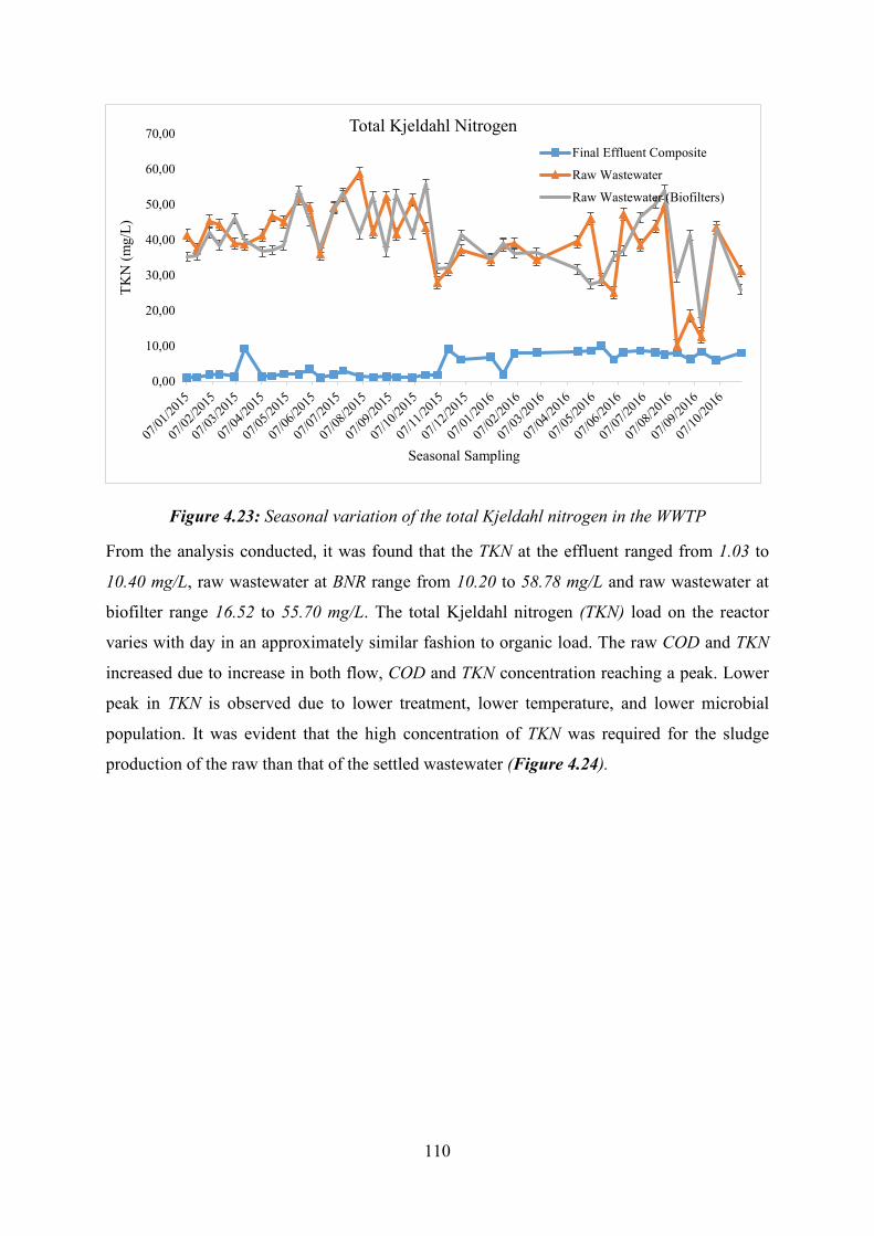
110

Figure 4.23: Seasonal variation of the total Kjeldahl nitrogen in the WWTP

From the analysis conducted, it was found that the TKN at the effluent ranged from 1.03 to

10.40 mg/L, raw wastewater at BNR range from 10.20 to 58.78 mg/L and raw wastewater at

biofilter range 16.52 to 55.70 mg/L. The total Kjeldahl nitrogen (TKN) load on the reactor

varies with day in an approximately similar fashion to organic load. The raw COD and TKN

increased due to increase in both flow, COD and TKN concentration reaching a peak. Lower

peak in TKN is observed due to lower treatment, lower temperature, and lower microbial

population. It was evident that the high concentration of TKN was required for the sludge

production of the raw than that of the settled wastewater (Figure 4.24).

0,00

10,00

20,00

30,00

40,00

50,00

60,00

70,00TK

N (m

g/L)

Seasonal Sampling

Total Kjeldahl NitrogenFinal Effluent Composite

Raw Wastewater

Raw Wastewater (Biofilters)

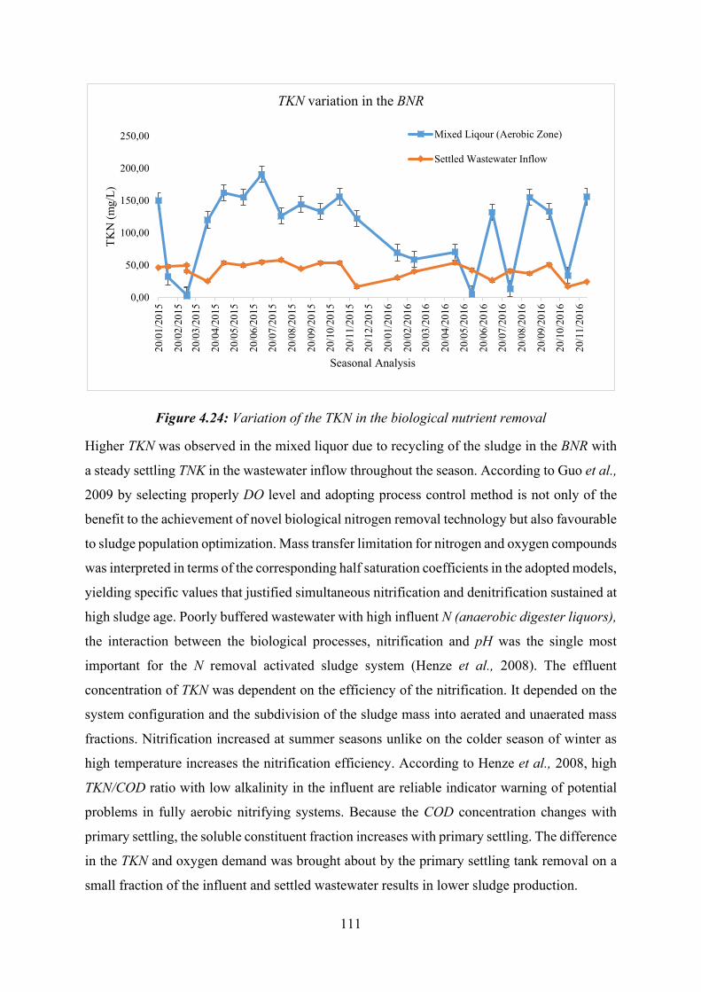
111

Figure 4.24: Variation of the TKN in the biological nutrient removal

Higher TKN was observed in the mixed liquor due to recycling of the sludge in the BNR with

a steady settling TNK in the wastewater inflow throughout the season. According to Guo et al.,

2009 by selecting properly DO level and adopting process control method is not only of the

benefit to the achievement of novel biological nitrogen removal technology but also favourable

to sludge population optimization. Mass transfer limitation for nitrogen and oxygen compounds

was interpreted in terms of the corresponding half saturation coefficients in the adopted models,

yielding specific values that justified simultaneous nitrification and denitrification sustained at

high sludge age. Poorly buffered wastewater with high influent N (anaerobic digester liquors),

the interaction between the biological processes, nitrification and pH was the single most

important for the N removal activated sludge system (Henze et al., 2008). The effluent

concentration of TKN was dependent on the efficiency of the nitrification. It depended on the

system configuration and the subdivision of the sludge mass into aerated and unaerated mass

fractions. Nitrification increased at summer seasons unlike on the colder season of winter as

high temperature increases the nitrification efficiency. According to Henze et al., 2008, high

TKN/COD ratio with low alkalinity in the influent are reliable indicator warning of potential

problems in fully aerobic nitrifying systems. Because the COD concentration changes with

primary settling, the soluble constituent fraction increases with primary settling. The difference

in the TKN and oxygen demand was brought about by the primary settling tank removal on a

small fraction of the influent and settled wastewater results in lower sludge production.

0,00

50,00

100,00

150,00

200,00

250,00

20/0

1/20

15

20/0

2/20

15

20/0

3/20

15

20/0

4/20

15

20/0

5/20

15

20/0

6/20

15

20/0

7/20

15

20/0

8/20

15

20/0

9/20

15

20/1

0/20

15

20/1

1/20

15

20/1

2/20

15

20/0

1/20

16

20/0

2/20

16

20/0

3/20

16

20/0

4/20

16

20/0

5/20

16

20/0

6/20

16

20/0

7/20

16

20/0

8/20

16

20/0

9/20

16

20/1

0/20

16

20/1

1/20

16

TKN

(mg/

L)

Seasonal Analysis

TKN variation in the BNR

Mixed Liqour (Aerobic Zone)

Settled Wastewater Inflow

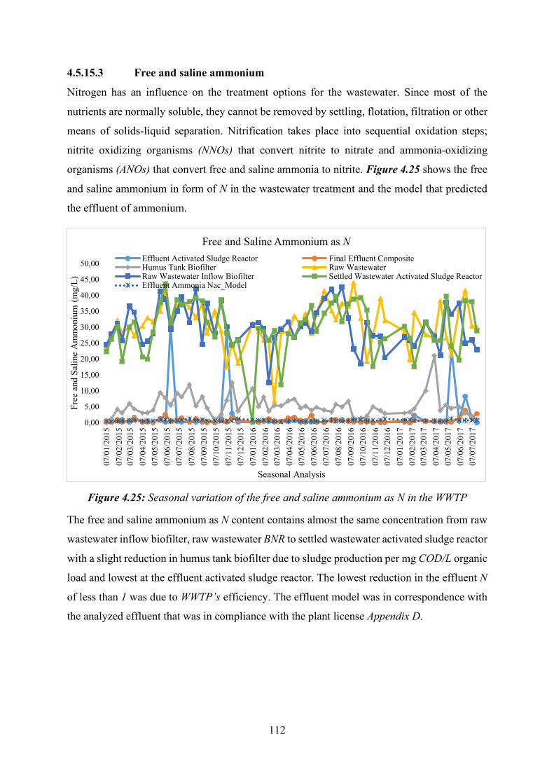
112

4.5.15.3 Free and saline ammonium

Nitrogen has an influence on the treatment options for the wastewater. Since most of the

nutrients are normally soluble, they cannot be removed by settling, flotation, filtration or other

means of solids-liquid separation. Nitrification takes place into sequential oxidation steps;

nitrite oxidizing organisms (NNOs) that convert nitrite to nitrate and ammonia-oxidizing

organisms (ANOs) that convert free and saline ammonia to nitrite. Figure 4.25 shows the free

and saline ammonium in form of N in the wastewater treatment and the model that predicted

the effluent of ammonium.

Figure 4.25: Seasonal variation of the free and saline ammonium as N in the WWTP

The free and saline ammonium as N content contains almost the same concentration from raw

wastewater inflow biofilter, raw wastewater BNR to settled wastewater activated sludge reactor

with a slight reduction in humus tank biofilter due to sludge production per mg COD/L organic

load and lowest at the effluent activated sludge reactor. The lowest reduction in the effluent N

of less than 1 was due to WWTP’s efficiency. The effluent model was in correspondence with

the analyzed effluent that was in compliance with the plant license Appendix D.

0,00

5,00

10,00

15,00

20,00

25,00

30,00

35,00

40,00

45,00

50,00

07/0

1/20

1507

/02/

2015

07/0

3/20

1507

/04/

2015

07/0

5/20

1507

/06/

2015

07/0

7/20

1507

/08/

2015

07/0

9/20

1507

/10/

2015

07/1

1/20

1507

/12/

2015

07/0

1/20

1607

/02/

2016

07/0

3/20

1607

/04/

2016

07/0

5/20

1607

/06/

2016

07/0

7/20

1607

/08/

2016

07/0

9/20

1607

/10/

2016

07/1

1/20

1607

/12/

2016

07/0

1/20

1707

/02/

2017

07/0

3/20

1707

/04/

2017

07/0

5/20

1707

/06/

2017

07/0

7/20

17

Free

and

Sal

ine

Am

mon

ium

(mg/

L)

Seasonal Analysis

Free and Saline Ammonium as NEffluent Activated Sludge Reactor Final Effluent CompositeHumus Tank Biofilter Raw WastewaterRaw Wastewater Inflow Biofilter Settled Wastewater Activated Sludge ReactorEffluent Ammonia Nac_Model

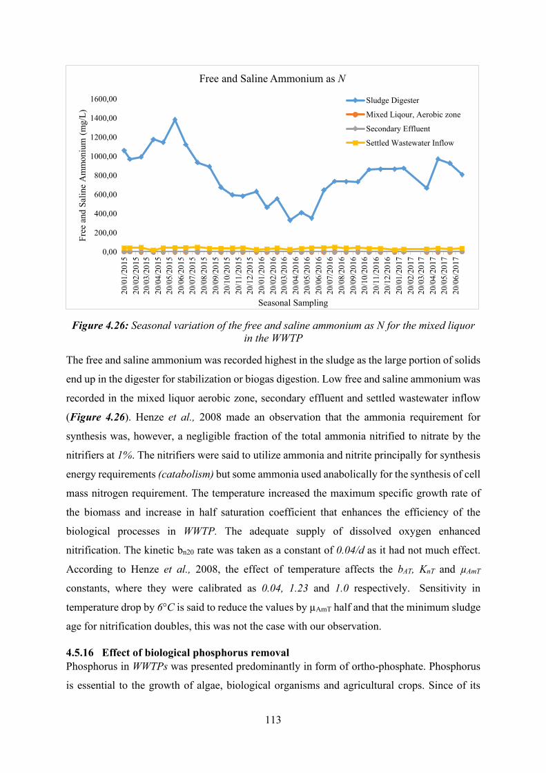
113

Figure 4.26: Seasonal variation of the free and saline ammonium as N for the mixed liquor in the WWTP

The free and saline ammonium was recorded highest in the sludge as the large portion of solids

end up in the digester for stabilization or biogas digestion. Low free and saline ammonium was

recorded in the mixed liquor aerobic zone, secondary effluent and settled wastewater inflow

(Figure 4.26). Henze et al., 2008 made an observation that the ammonia requirement for

synthesis was, however, a negligible fraction of the total ammonia nitrified to nitrate by the

nitrifiers at 1%. The nitrifiers were said to utilize ammonia and nitrite principally for synthesis

energy requirements (catabolism) but some ammonia used anabolically for the synthesis of cell

mass nitrogen requirement. The temperature increased the maximum specific growth rate of

the biomass and increase in half saturation coefficient that enhances the efficiency of the

biological processes in WWTP. The adequate supply of dissolved oxygen enhanced

nitrification. The kinetic bn20 rate was taken as a constant of 0.04/d as it had not much effect.

According to Henze et al., 2008, the effect of temperature affects the bAT, KnT and µAmT

constants, where they were calibrated as 0.04, 1.23 and 1.0 respectively. Sensitivity in

temperature drop by 6°C is said to reduce the values by µAmT half and that the minimum sludge

age for nitrification doubles, this was not the case with our observation.

4.5.16 Effect of biological phosphorus removal Phosphorus in WWTPs was presented predominantly in form of ortho-phosphate. Phosphorus

is essential to the growth of algae, biological organisms and agricultural crops. Since of its

0,00

200,00

400,00

600,00

800,00

1000,00

1200,00

1400,00

1600,00

20/0

1/20

1520

/02/

2015

20/0

3/20

1520

/04/

2015

20/0

5/20

1520

/06/

2015

20/0

7/20

1520

/08/

2015

20/0

9/20

1520

/10/

2015

20/1

1/20

1520

/12/

2015

20/0

1/20

1620

/02/

2016

20/0

3/20

1620

/04/

2016

20/0

5/20

1620

/06/

2016

20/0

7/20

1620

/08/

2016

20/0

9/20

1620

/10/

2016

20/1

1/20

1620

/12/

2016

20/0

1/20

1720

/02/

2017

20/0

3/20

1720

/04/

2017

20/0

5/20

1720

/06/

2017

Free

and

Sal

ine

Am

mon

ium

(mg/

L)

Seasonal Sampling

Free and Saline Ammonium as N

Sludge Digester

Mixed Liqour, Aerobic zone

Secondary Effluent

Settled Wastewater Inflow

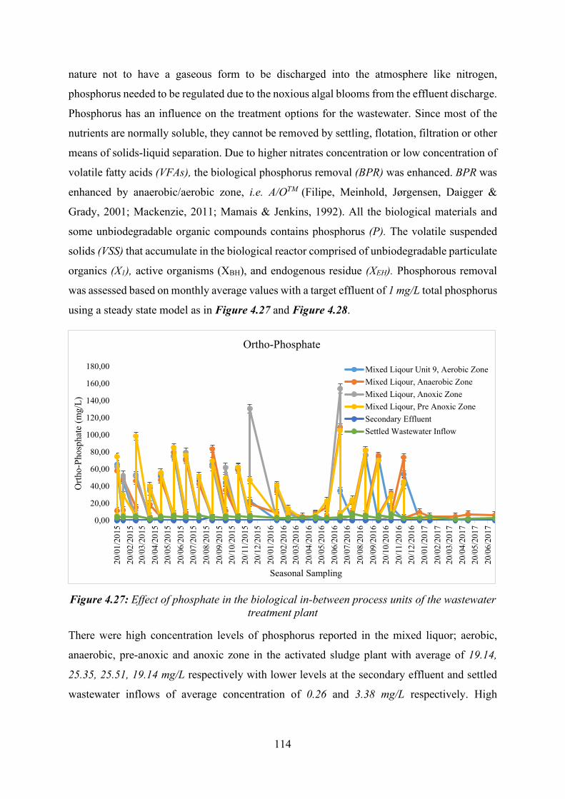
114

nature not to have a gaseous form to be discharged into the atmosphere like nitrogen,

phosphorus needed to be regulated due to the noxious algal blooms from the effluent discharge.

Phosphorus has an influence on the treatment options for the wastewater. Since most of the

nutrients are normally soluble, they cannot be removed by settling, flotation, filtration or other

means of solids-liquid separation. Due to higher nitrates concentration or low concentration of

volatile fatty acids (VFAs), the biological phosphorus removal (BPR) was enhanced. BPR was

enhanced by anaerobic/aerobic zone, i.e. A/OTM (Filipe, Meinhold, Jørgensen, Daigger &

Grady, 2001; Mackenzie, 2011; Mamais & Jenkins, 1992). All the biological materials and

some unbiodegradable organic compounds contains phosphorus (P). The volatile suspended

solids (VSS) that accumulate in the biological reactor comprised of unbiodegradable particulate

organics (X1), active organisms (XBH), and endogenous residue (XEH). Phosphorous removal

was assessed based on monthly average values with a target effluent of 1 mg/L total phosphorus

using a steady state model as in Figure 4.27 and Figure 4.28.

Figure 4.27: Effect of phosphate in the biological in-between process units of the wastewater treatment plant

There were high concentration levels of phosphorus reported in the mixed liquor; aerobic,

anaerobic, pre-anoxic and anoxic zone in the activated sludge plant with average of 19.14,

25.35, 25.51, 19.14 mg/L respectively with lower levels at the secondary effluent and settled

wastewater inflows of average concentration of 0.26 and 3.38 mg/L respectively. High

0,00

20,00

40,00

60,00

80,00

100,00

120,00

140,00

160,00

180,00

20/0

1/20

1520

/02/

2015

20/0

3/20

1520

/04/

2015

20/0

5/20

1520

/06/

2015

20/0

7/20

1520

/08/

2015

20/0

9/20

1520

/10/

2015

20/1

1/20

1520

/12/

2015

20/0

1/20

1620

/02/

2016

20/0

3/20

1620

/04/

2016

20/0

5/20

1620

/06/

2016

20/0

7/20

1620

/08/

2016

20/0

9/20

1620

/10/

2016

20/1

1/20

1620

/12/

2016

20/0

1/20

1720

/02/

2017

20/0

3/20

1720

/04/

2017

20/0

5/20

1720

/06/

2017

Orth

o-Ph

osph

ate

(mg/

L)

Seasonal Sampling

Ortho-Phosphate

Mixed Liqour Unit 9, Aerobic ZoneMixed Liqour, Anaerobic ZoneMixed Liqour, Anoxic ZoneMixed Liqour, Pre Anoxic ZoneSecondary EffluentSettled Wastewater Inflow

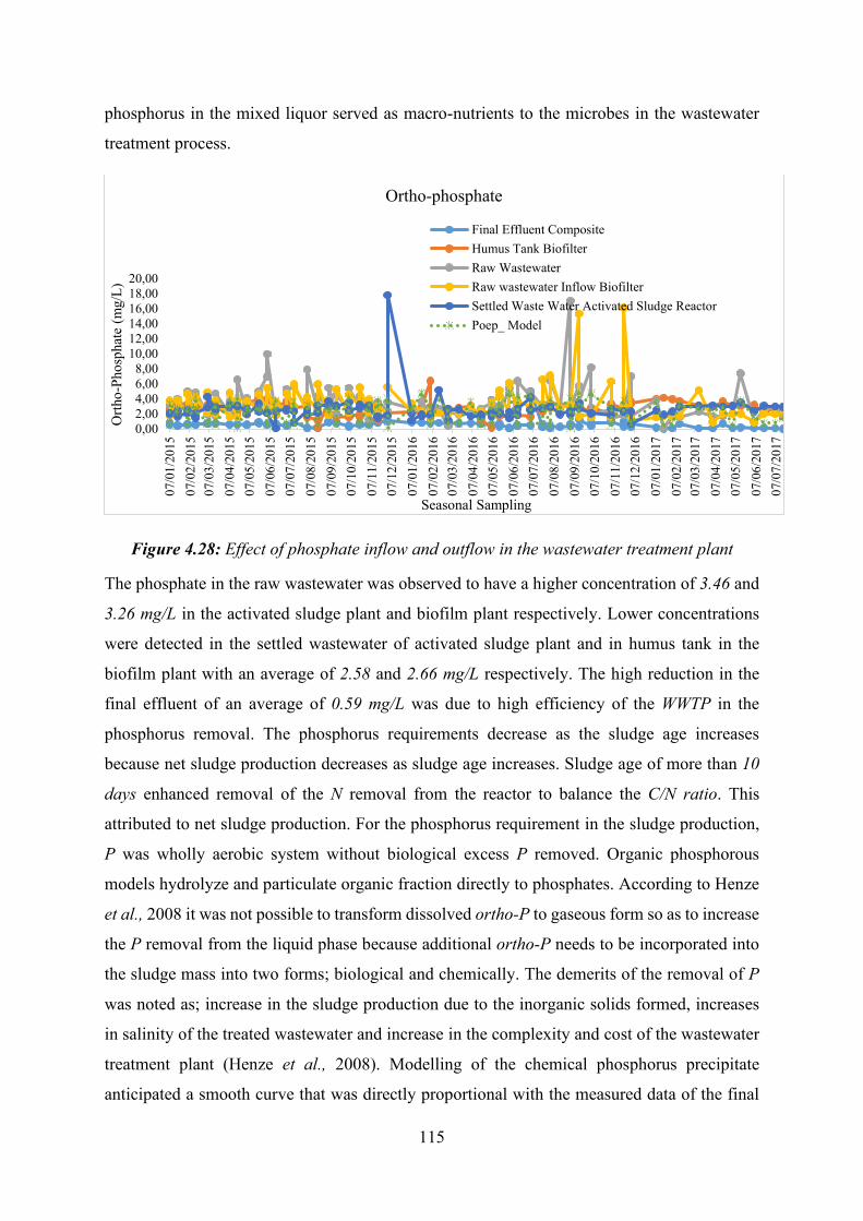
115

phosphorus in the mixed liquor served as macro-nutrients to the microbes in the wastewater

treatment process.

Figure 4.28: Effect of phosphate inflow and outflow in the wastewater treatment plant

The phosphate in the raw wastewater was observed to have a higher concentration of 3.46 and

3.26 mg/L in the activated sludge plant and biofilm plant respectively. Lower concentrations

were detected in the settled wastewater of activated sludge plant and in humus tank in the

biofilm plant with an average of 2.58 and 2.66 mg/L respectively. The high reduction in the

final effluent of an average of 0.59 mg/L was due to high efficiency of the WWTP in the

phosphorus removal. The phosphorus requirements decrease as the sludge age increases

because net sludge production decreases as sludge age increases. Sludge age of more than 10

days enhanced removal of the N removal from the reactor to balance the C/N ratio. This

attributed to net sludge production. For the phosphorus requirement in the sludge production,

P was wholly aerobic system without biological excess P removed. Organic phosphorous

models hydrolyze and particulate organic fraction directly to phosphates. According to Henze

et al., 2008 it was not possible to transform dissolved ortho-P to gaseous form so as to increase

the P removal from the liquid phase because additional ortho-P needs to be incorporated into

the sludge mass into two forms; biological and chemically. The demerits of the removal of P

was noted as; increase in the sludge production due to the inorganic solids formed, increases

in salinity of the treated wastewater and increase in the complexity and cost of the wastewater

treatment plant (Henze et al., 2008). Modelling of the chemical phosphorus precipitate

anticipated a smooth curve that was directly proportional with the measured data of the final

0,002,004,006,008,00

10,0012,0014,0016,0018,0020,00

07/0

1/20

1507

/02/

2015

07/0

3/20

1507

/04/

2015

07/0

5/20

1507

/06/

2015

07/0

7/20

1507

/08/

2015

07/0

9/20

1507

/10/

2015

07/1

1/20

1507

/12/

2015

07/0

1/20

1607

/02/

2016

07/0

3/20

1607

/04/

2016

07/0

5/20

1607

/06/

2016

07/0

7/20

1607

/08/

2016

07/0

9/20

1607

/10/

2016

07/1

1/20

1607

/12/

2016

07/0

1/20

1707

/02/

2017

07/0

3/20

1707

/04/

2017

07/0

5/20

1707

/06/

2017

07/0

7/20

17

Orth

o-Ph

osph

ate

(mg/

L)

Seasonal Sampling

Ortho-phosphate

Final Effluent CompositeHumus Tank BiofilterRaw WastewaterRaw wastewater Inflow BiofilterSettled Waste Water Activated Sludge ReactorPoep_ Model

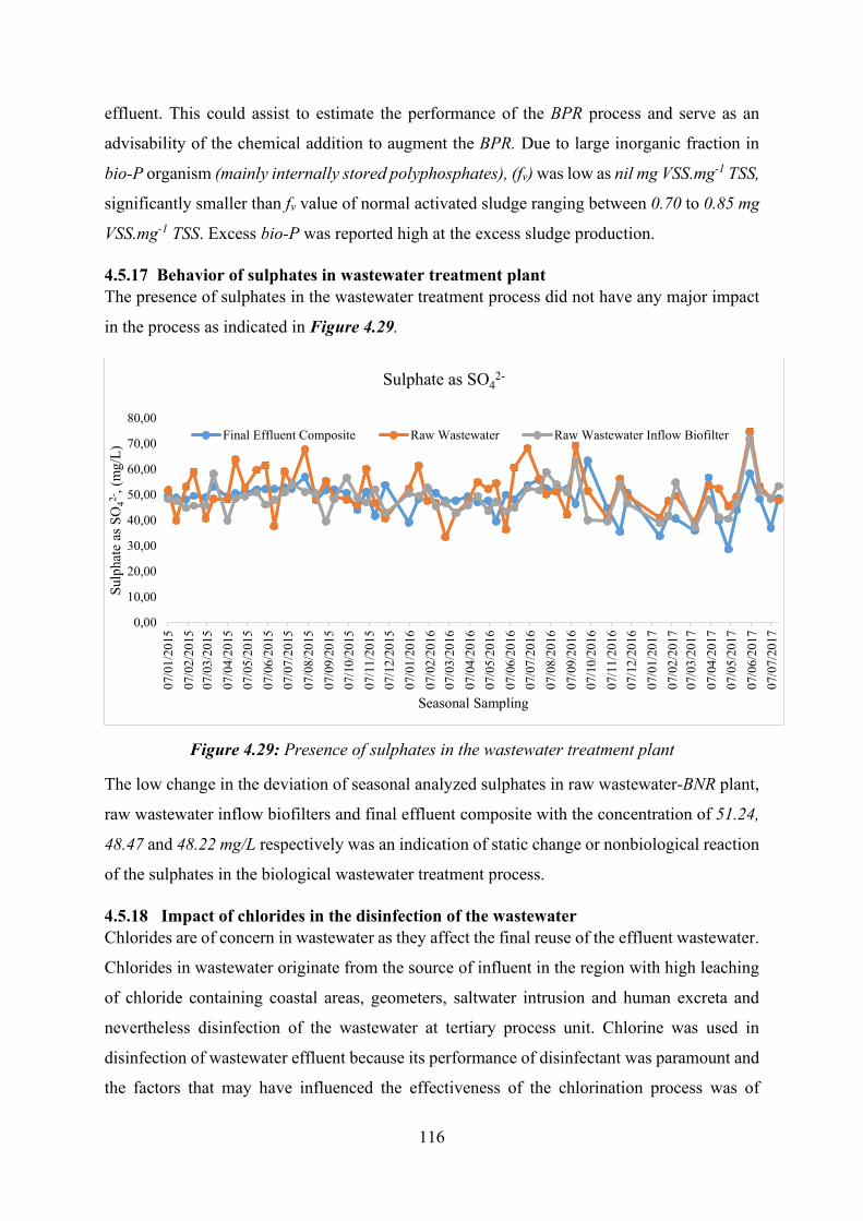
116

effluent. This could assist to estimate the performance of the BPR process and serve as an

advisability of the chemical addition to augment the BPR. Due to large inorganic fraction in

bio-P organism (mainly internally stored polyphosphates), (fv) was low as nil mg VSS.mg-1 TSS,

significantly smaller than fv value of normal activated sludge ranging between 0.70 to 0.85 mg

VSS.mg-1 TSS. Excess bio-P was reported high at the excess sludge production.

4.5.17 Behavior of sulphates in wastewater treatment plant The presence of sulphates in the wastewater treatment process did not have any major impact

in the process as indicated in Figure 4.29.

Figure 4.29: Presence of sulphates in the wastewater treatment plant

The low change in the deviation of seasonal analyzed sulphates in raw wastewater-BNR plant,

raw wastewater inflow biofilters and final effluent composite with the concentration of 51.24,

48.47 and 48.22 mg/L respectively was an indication of static change or nonbiological reaction

of the sulphates in the biological wastewater treatment process.

4.5.18 Impact of chlorides in the disinfection of the wastewater Chlorides are of concern in wastewater as they affect the final reuse of the effluent wastewater.

Chlorides in wastewater originate from the source of influent in the region with high leaching

of chloride containing coastal areas, geometers, saltwater intrusion and human excreta and

nevertheless disinfection of the wastewater at tertiary process unit. Chlorine was used in

disinfection of wastewater effluent because its performance of disinfectant was paramount and

the factors that may have influenced the effectiveness of the chlorination process was of

0,00

10,00

20,00

30,00

40,00

50,00

60,00

70,00

80,00

07/0

1/20

1507

/02/

2015

07/0

3/20

1507

/04/

2015

07/0

5/20

1507

/06/

2015

07/0

7/20

1507

/08/

2015

07/0

9/20

1507

/10/

2015

07/1

1/20

1507

/12/

2015

07/0

1/20

1607

/02/

2016

07/0

3/20

1607

/04/

2016

07/0

5/20

1607

/06/

2016

07/0

7/20

1607

/08/

2016

07/0

9/20

1607

/10/

2016

07/1

1/20

1607

/12/

2016

07/0

1/20

1707

/02/

2017

07/0

3/20

1707

/04/

2017

07/0

5/20

1707

/06/

2017

07/0

7/20

17

Sulp

hate

as S

O42-

, (m

g/L)

Seasonal Sampling

Sulphate as SO42-

Final Effluent Composite Raw Wastewater Raw Wastewater Inflow Biofilter

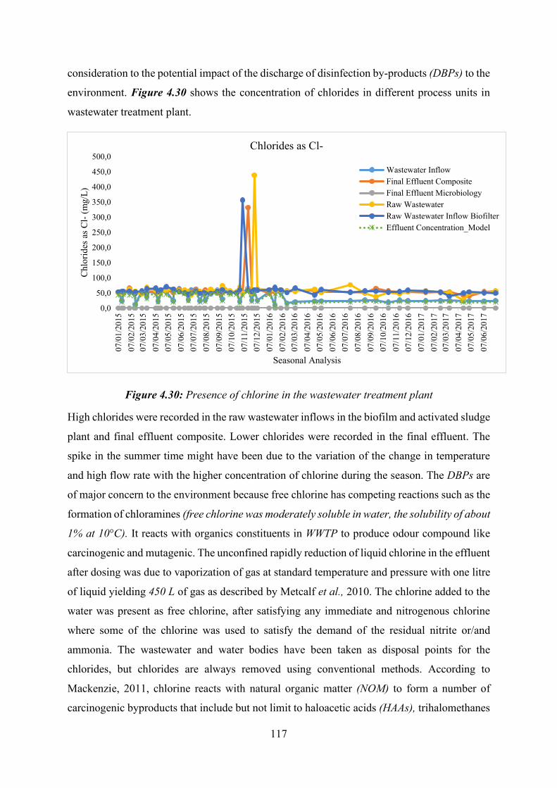
117

consideration to the potential impact of the discharge of disinfection by-products (DBPs) to the

environment. Figure 4.30 shows the concentration of chlorides in different process units in

wastewater treatment plant.

Figure 4.30: Presence of chlorine in the wastewater treatment plant

High chlorides were recorded in the raw wastewater inflows in the biofilm and activated sludge

plant and final effluent composite. Lower chlorides were recorded in the final effluent. The

spike in the summer time might have been due to the variation of the change in temperature

and high flow rate with the higher concentration of chlorine during the season. The DBPs are

of major concern to the environment because free chlorine has competing reactions such as the

formation of chloramines (free chlorine was moderately soluble in water, the solubility of about

1% at 10°C). It reacts with organics constituents in WWTP to produce odour compound like

carcinogenic and mutagenic. The unconfined rapidly reduction of liquid chlorine in the effluent

after dosing was due to vaporization of gas at standard temperature and pressure with one litre

of liquid yielding 450 L of gas as described by Metcalf et al., 2010. The chlorine added to the

water was present as free chlorine, after satisfying any immediate and nitrogenous chlorine

where some of the chlorine was used to satisfy the demand of the residual nitrite or/and

ammonia. The wastewater and water bodies have been taken as disposal points for the

chlorides, but chlorides are always removed using conventional methods. According to

Mackenzie, 2011, chlorine reacts with natural organic matter (NOM) to form a number of

carcinogenic byproducts that include but not limit to haloacetic acids (HAAs), trihalomethanes

0,0

50,0

100,0

150,0

200,0

250,0

300,0

350,0

400,0

450,0

500,0

07/0

1/20

1507

/02/

2015

07/0

3/20

1507

/04/

2015

07/0

5/20

1507

/06/

2015

07/0

7/20

1507

/08/

2015

07/0

9/20

1507

/10/

2015

07/1

1/20

1507

/12/

2015

07/0

1/20

1607

/02/

2016

07/0

3/20

1607

/04/

2016

07/0

5/20

1607

/06/

2016

07/0

7/20

1607

/08/

2016

07/0

9/20

1607

/10/

2016

07/1

1/20

1607

/12/

2016

07/0

1/20

1707

/02/

2017

07/0

3/20

1707

/04/

2017

07/0

5/20

1707

/06/

2017

Chl

orid

es a

s Cl-

(mg/

L)

Seasonal Analysis

Chlorides as Cl-

Wastewater InflowFinal Effluent CompositeFinal Effluent MicrobiologyRaw WastewaterRaw Wastewater Inflow BiofilterEffluent Concentration_Model

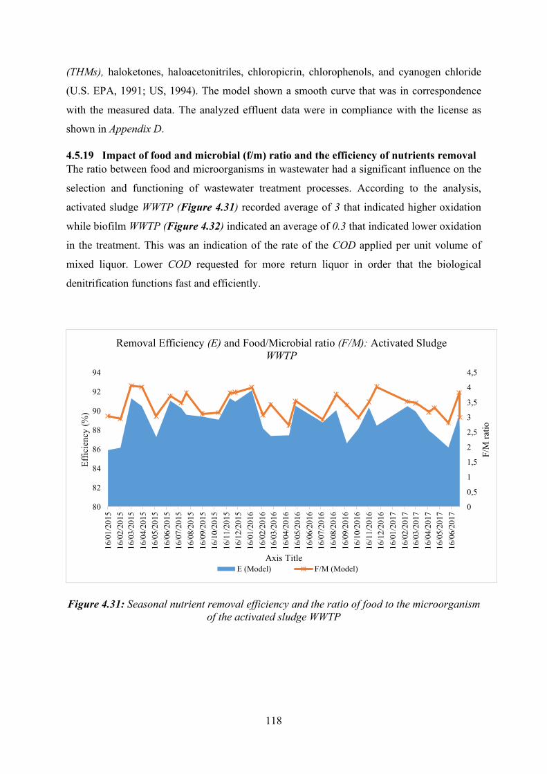
118

(THMs), haloketones, haloacetonitriles, chloropicrin, chlorophenols, and cyanogen chloride

(U.S. EPA, 1991; US, 1994). The model shown a smooth curve that was in correspondence

with the measured data. The analyzed effluent data were in compliance with the license as

shown in Appendix D.

4.5.19 Impact of food and microbial (f/m) ratio and the efficiency of nutrients removal The ratio between food and microorganisms in wastewater had a significant influence on the

selection and functioning of wastewater treatment processes. According to the analysis,

activated sludge WWTP (Figure 4.31) recorded average of 3 that indicated higher oxidation

while biofilm WWTP (Figure 4.32) indicated an average of 0.3 that indicated lower oxidation

in the treatment. This was an indication of the rate of the COD applied per unit volume of

mixed liquor. Lower COD requested for more return liquor in order that the biological

denitrification functions fast and efficiently.

Figure 4.31: Seasonal nutrient removal efficiency and the ratio of food to the microorganism of the activated sludge WWTP

0

0,5

1

1,5

2

2,5

3

3,5

4

4,5

80

82

84

86

88

90

92

94

16/0

1/20

1516

/02/

2015

16/0

3/20

1516

/04/

2015

16/0

5/20

1516

/06/

2015

16/0

7/20

1516

/08/

2015

16/0

9/20

1516

/10/

2015

16/1

1/20

1516

/12/

2015

16/0

1/20

1616

/02/

2016

16/0

3/20

1616

/04/

2016

16/0

5/20

1616

/06/

2016

16/0

7/20

1616

/08/

2016

16/0

9/20

1616

/10/

2016

16/1

1/20

1616

/12/

2016

16/0

1/20

1716

/02/

2017

16/0

3/20

1716

/04/

2017

16/0

5/20

1716

/06/

2017

F/M

ratio

Effic

ienc

y (%

)

Axis Title

Removal Efficiency (E) and Food/Microbial ratio (F/M): Activated Sludge WWTP

E (Model) F/M (Model)

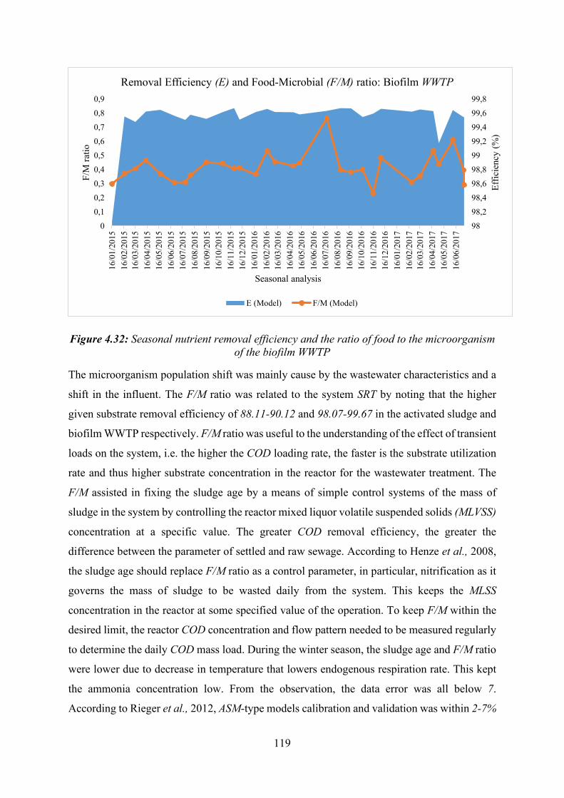
119

Figure 4.32: Seasonal nutrient removal efficiency and the ratio of food to the microorganism of the biofilm WWTP

The microorganism population shift was mainly cause by the wastewater characteristics and a

shift in the influent. The F/M ratio was related to the system SRT by noting that the higher

given substrate removal efficiency of 88.11-90.12 and 98.07-99.67 in the activated sludge and

biofilm WWTP respectively. F/M ratio was useful to the understanding of the effect of transient

loads on the system, i.e. the higher the COD loading rate, the faster is the substrate utilization

rate and thus higher substrate concentration in the reactor for the wastewater treatment. The

F/M assisted in fixing the sludge age by a means of simple control systems of the mass of

sludge in the system by controlling the reactor mixed liquor volatile suspended solids (MLVSS)

concentration at a specific value. The greater COD removal efficiency, the greater the

difference between the parameter of settled and raw sewage. According to Henze et al., 2008,

the sludge age should replace F/M ratio as a control parameter, in particular, nitrification as it

governs the mass of sludge to be wasted daily from the system. This keeps the MLSS

concentration in the reactor at some specified value of the operation. To keep F/M within the

desired limit, the reactor COD concentration and flow pattern needed to be measured regularly

to determine the daily COD mass load. During the winter season, the sludge age and F/M ratio

were lower due to decrease in temperature that lowers endogenous respiration rate. This kept

the ammonia concentration low. From the observation, the data error was all below 7.

According to Rieger et al., 2012, ASM-type models calibration and validation was within 2-7%

9898,298,498,698,89999,299,499,699,8

00,10,20,30,40,50,60,70,80,9

16/0

1/20

1516

/02/

2015

16/0

3/20

1516

/04/

2015

16/0

5/20

1516

/06/

2015

16/0

7/20

1516

/08/

2015

16/0

9/20

1516

/10/

2015

16/1

1/20

1516

/12/

2015

16/0

1/20

1616

/02/

2016

16/0

3/20

1616

/04/

2016

16/0

5/20

1616

/06/

2016

16/0

7/20

1616

/08/

2016

16/0

9/20

1616

/10/

2016

16/1

1/20

1616

/12/

2016

16/0

1/20

1716

/02/

2017

16/0

3/20

1716

/04/

2017

16/0

5/20

1716

/06/

2017

Effic

ienc

y (%

)

F/M

ratio

Seasonal analysis

Removal Efficiency (E) and Food-Microbial (F/M) ratio: Biofilm WWTP

E (Model) F/M (Model)

120

of high-quality data, except at very low effluent concentrations where the acceptable margin

was higher.

4.6 Conclusion

Wastewater treatment process can be considered as the largest industry in terms of waste

management industries. The biological behaviour of biotechnological processes occurring in a

bioreactor has a complexity unparalleled in the chemistry application principles. The complex

systems, therefore, resulted in the involvement of the models based on the mathematical

description of the process after the off-line sampling and analysis due to lack of the on-line

sensor. The study applied practical knowledge of IAWQ Activated Sludge Model No.1 and

mass balance through a database that combines experience from expert knowledge and

modelling experience. The basis for the development of reliable mathematical models was the

thorough understanding of the involved process. Activated sludge systems were described by

mathematical models based on mass balance equations that relate to change of the state

variables of the system (flow rates, concentration and composition) due to transport and the

transformation mechanisms. The authors combine the ASM1 principles, substrate and

microorganisms’ kinetics in mass balance and thus resulting in a standardized methodology for

expressing nomenclature that is useful for the WWTP modellers and other experts. This will

enhance coding in the programming of the simulation software by eliminating error-prone part

of the model implementation. The spreadsheet provided corrected matrices with all

stoichiometric coefficient for the bio-kinetic models. The presence of emerging micro-

pollutants (methylparabens, ethylparabens, propylparabens) and the inclusion of water

chemistry indicated that the plant has the capability and is effective in removing the fate of

micro-pollutants. COD mass balance made a lot of sense on the prediction of the experimental

data that was reliable and accurate. Monitoring the reactor concentration and its changes at a

fixed parameter created a long-term change in the loading rate on the WWTP and thus increase

its efficiency. The structured framework of the models was useful among modellers, operators

and management at the WWTPs, and other wastewater stakeholders. The models provided

guidance in identifying the key design parameters and quantify system parameters that ensured

optimal performance. The information provided an insight into the wastewater characteristic

that included; biodegradability, flow distribution, contaminants and potential for the source

control. These models provided the quantitative predictions of quality of effluent to be expected

from a design of the existing WWTP and guidance to the direct attention needed in the system

and control response. Use of the ASM1 facilitated communication of the complex models and

121

allowed the concentration of discussion on the bio-kinetics models. Mass balance was a

powerful tool that allowed detection of inconsistencies within the WWTP data sets and assists

to identify the systematic errors. The models were verified by conforming to internal mass

balance and adequate validation against the experimental tests. The results contributed to the

knowledge transfer on activated sludge and biofilm modelling.

122

CHAPTER 5: TRACE METALS SPECIATION MODELLING IN THE

WASTEWATER TREATMENT PROCESSES: GEOCHEMICAL MODELLING

5.1 Summary

The speciation of trace metals in the wastewater treatment plants (WWTPs) determines its

ultimate fate in natural surface waters due to biological and chemical processes. The

quantification of the trace metals speciation studies was undertaken in the influent and effluent

of the WWTP and was of special concern due to their persistence and recalcitrance in the

biosphere. The metals of interest included: Al, Cd, Co, Cr, Cu, Fe, Mn, Mo, Ni, Pb, Ti and Zn.

Trace metals accumulated dependent and independent on metabolism; the biomass as well as

in cellular products such as polysaccharides for metals removal were determined using

geochemical modelling-mass balance. The mass balance model had a numerical cost

optimization procedure that uses steady state together with a set of predefined constraints to

evaluate operation points, plant dimensions and controller parameters. Mass balance model

allowed detection of inconsistencies within the trace metals datasets and assisted in identifying

the systematic errors in the metal reduction to quantify the overall removal and fate of these

compounds in biological treatment plants. Mass balance comprising of seasonal programmable

sampling showed a significant reduction in the number of trace metals. Removal of metals from

biological treatment processes was mainly by complexation of the metals with microorganisms,

precipitation and adsorption. The comparison of the available measured data indicated an

increasing trend of high concentration in the sludge (biomass) that could be of danger to the

human population, flora and fauna of the receiving water bodies. Geochemical modelling and

computation of the speciation of the trace metals offer an extremely powerful tool for the

process design, troubleshooting and optimization representing a multivariable system that

cannot be effectively handled without appropriate modelling and computer-based techniques.

5.2 Introduction

The accelerating industrialization and urban activities in developing countries (mining and

commercial region) introduces a significant amount of pollutants (organics, inorganics,

emerging contaminants, trace metals, etc.) into the water systems, consequently ecological

123

degradation, environmental and causing a high anthropogenic emission of the pollutants into

the biosphere (Cheng, Grosse, Karrenbrock & Thoennessen, 2002; Kamika, Coetzee, Mamba,

Msagati & Momba, 2014). In the recent years, trace metals production emission has decreased

in many countries due to legislation, improved cleaning technology and altered industrial

activities (Karvelas et al., 2003). With the fourth industrial revolution (FIR), the exponentially

increasing population push a need for controlling trace metals speciation into the environment

in a more pronounced due to the high level of toxicity, bioaccumulation and wide range of

source and persistence (Wang et al., 2015). The xenobiotic of the trace metals allows them to

accumulate in the environment (Burgess, Quarmby & Stephenson, 1999). To follow the fate of

metallic species after that have intensified environmental pollution and deteriorate the

ecosystems, with the accumulation of pollutants that has become persistence and recalcitrance

in the biosphere (Veglio & Beolchini, 1997; Volesky, 2001). This results in health problems

that demonstrate themselves on the acute as well as chronic levels that reflected in the society’s

spiraling health care cost (Volesky, 2001). The hazardous of trace metals pollution of

wastewater to the environment is well explained by Fu and Wang (2011) (Fu & Wang, 2011).

Growing attention has been given to the potential health hazard presented by the trace metals

to the environment. Another emerging technological advancement (nanotechnology) with a

sparkling bright future has nanoparticles entering water streams and wastewater treatment

process (Shamuyarira & Gumbo, 2014). Mining industries and industrial activities have been

considered as major sources of trace metals contaminants. The trace metals can be precipitated,

dissolved, co-precipitated with metal oxides, adsorbed or involve in microbial metabolism.

Trace metals can be found in form of hydroxides, oxides, sulphide, silicates, sulphates, organic

binding forming complexes with humic compounds and complex sugar (Gawdzik & Gawdzik,

2012). To eliminate the environmental hazards associated with the trace metals wastewater

steams should be treated using a robust technique (Singanan & Peters, 2013). The current

economic, technical, effective conventional treatment technologies processes for the removal

of the trace metals include: membrane technology, flotation, oxidation, electrodialysis,

photocatalysis, coagulation-flocculation, ion-exchange, electrochemical, adsorption, chemical

precipitation and biological process-microbial biomass (biosorption) based on trace metals

binding capacities of various biological matters (where bacteria, algae, yeast and fungi has

proved to be potential metal sorbents) (Barakat, 2011; Davis, Volesky & Mucci, 2003; Fu &

Wang, 2011; Mohan & Pittman Jr, 2007; Sheoran & Sheoran, 2006; Veglio & Beolchini, 1997).

The life cycle assessment (LCA) is put in place to analyze the environmental impact of different

technologies for the wastewater treatment in the populations. Gallego, Hospido, Moreira &

124

Feijoo, 2008 describe LCA as an environmental tool that allows the calculation of all the

environmental loads related to a service/process/product. It is thus important to treat trace

metals contaminated wastewater prior to its discharge to the environment.

Besides the hazard posed by the high-level concentration of trace metals, WWTPs contain also

necessary nutrients for the cell growth in microbiology within the concentration threshold

(Karlsson et al., 2012; Matheri, Mbohwa, Belaid, Seodigeng & Ngila, 2016; Schattauer,

Abdoun, Weiland, Plöchl & Heiermann, 2011; L. Zhang, Ouyang & Lia, 2012). Many of the

trace metals are important micro-nutrients and acts as microbial agents (enzyme and co-

enzyme) however, an excessive amount may result in toxicity or inhibition (Bożym, Florczak,

Zdanowska, Wojdalski & Klimkiewicz, 2015; Edokpayi, Odiyo, Popoola & Msagati, 2016;

Schattauer et al., 2011). Trace metals are adsorbed to the surface of negatively charged bacteria

fibrils that extend into bulk solution from cells membrane through cell walls. The fibrils are

negatively charged by the ionization from key functional groups such as hydroxyl-OH and

COOH. Once adsorbed, trace metals are absorbed by bacterial cells. The inside cells trace

metals attack enzyme systems. Trace metals toxicity is believed to occur through the structure

disruption of the enzymes and proteins molecules with the cells. Zhang et al., 2012 reported

that selected trace metals are limiting factor when included in co-enzymes, where the cells’

synthesis is seriously affected by the deficiency, or cell become more sensitive to inhibitory

substances. Meanwhile, the trace metals are valuable resources that should be recovered as

much as possible from the waste (Wang, Lu & Li, 2016). The maximum acceptance

concentrations are regulated by the wastewater treatment plant license compliance, World

Health Organization (WHO), US. Environmental Protection Agency (EPA), Agency for Toxic

Substances and Diseases Registry (ATSDR) among others (Abdel-Shafy & Mansour, 2014;

Department of Water and Sanitation, [Accessed June 2016]; Raval, Shah & Shah, 2016).

5.3 Geochemical Modelling

Modelling the fate of transport and occurrence of the micro-pollutants (i.e. trace metal) through

the wastewater treatment plants is of the present concern (Pomiès, Choubert, Wisniewski &

Coquery, 2013). Geochemical modelling and computation of the speciation of the trace metals

offer an extremely powerful tool for the process design, troubleshooting and optimization

representing a multivariable system cannot be effectively handled without appropriate

modelling and computer-based techniques (Volesky, 2001). The modelling assumes basic mass

125

balance principles (model-based predictive) and simple reaction kinetics (Srivastava &

Majumder, 2008). The mass balance has a numerical cost optimization procedure that uses

steady state or dynamic state together with a set of predefined constraints to evaluate operation

points, plant dimensions and controller parameters. The constraints are selected to ensure that

process variable and some controllability measures lie within specified bounds (Vega,

Alawneh, Gonzalez, Francisco & Perez). The mass balance is valuable tools for investigating

the general performance of the wastewater treatment plants and an effective method to assess

the reliability of the available data (Gans, Mobini & Zhang). According to Sötemann, Wentzel

& Ekama, 2006, the primary purpose of the steady-state model is to determine the fate of

transport of trace metals, organic, organic and emerging contaminants, reactor volume, sludge

age, oxygen demand or gas production of the main biological process units in WWTP. Once

the parameters are determined, the individual process units can be modelled with the simulation

models to check their load response, cyclic flow and performance. The step for modelling

consists of the definition of the objectives, collection of the plant routine data and model

selection, data quality control, evaluation of the model structure and experimental design, data

collection for simulation study, and lastly calibration and validation (Langergraber et al.,

2004b).

The objective of the study was to predict the occurrence, fate and transport of the speciation

trace metals in the wastewater treatment plant by carrying out a geochemical modelling using

a mass balance.

5.4 Material and Methods

Sampling was undertaken from the inflow and outflow of the Daspoort wastewater treatment

plant, Gauteng Province, South Africa. The sampling points were division box, primary

clarifier (settler), biological nutrients removal (BNR) for activated sludge WWTP or trickling

filter for the biofilm WWTP, humus tank, and chlorine contact dam (CCT). The samples were

collected in 500 mL plastic containers with no headspace volume to minimise aerobic

biodegradation of organics substrates. They were marked with the indication of time, date and

location of collection. Aliquots for trace metals analysis were acidified to a pH of about 2 with

nitric acid (16 M) and stored in the dark at 4°C. This was to protect trace metals from

precipitation and sorption losses to the container walls (Mackenzie, 2011; Metcalf et al., 2010).

126

5.4.1 Analytical methods for trace metals

Sample preparation methods for trace metals analysis involved using nitric acid (12 mL) and

hydrogen peroxide (4 mL) for digestion of the sample (10 mL) by hot plate digestion at 120°C

for 2 hours. Deionized water was added to dilute the sample and make 100 mL after digestion.

The sample was then filtered using cellulose acetate membrane filter (0.22 µm). The classes of

metals were: suspended metals, metals present in unacidified samples that are retained on the

0.45 µm membrane filter; dissolved metals, present in unacidified samples that pass through a

0.45 µm membrane filter; total metals, the total of the dissolved and suspended metals or the

concentration of metals determined on an unfiltered sample after digestion, and lastly acid

extractable metals, metals in solution after an unfiltered sample is treated with a hot dilute

mineral acids according to the standard method (Beamish, 2012; Biller & Bruland, 2012).

Calibration standards were prepared using multi-element calibration solutions prepared using-

100 mg/L nitric acid and deionized water. The sample was then analysed using inductively

coupled plasma optical emission spectrometry (ICP-OES-model ICAP 6500 Duo) – (165

Spectro Arcos equipped with autosampler (Cetac ASX-520) technique. The parameters for

operating the ICP-OES was set as follows: instrument power 1400 W, the flow rate of the

auxiliary argon 2 L/min, argon gas flow rate 13 L/min, the flow rate of the argon nebuliser 0.95

L/min and iTEVA software was used. Based on the optical metals wavelength (lower

determination 166.250 nm and extending to 847.000 nm), the most prominent analytical lines

were chosen as follows: Al-396.152 nm, Cd-228.616.502 nm, Co-228.616 nm, Cr-283.565 nm,

Cu-324.754 nm, Fe-259.933 nm, Mn-257.610 nm, Ni-221.647 nm, Pb-220.353 nm, Ti-334.941

nm and Zn-213.856 nm. Dilution factor was applied to the concentration data. The trace metal

of interest included: Al, Cd, Co, Cr, Cu, Fe, Mn, Mo, Ni, Pb, Ti and Zn (Dimpe et al., 2014;

Scientific, 2009; Scientific., 2009; Wiel, 2003). Calculation of the concentration of the

elements in the aqueous sample and in the digested solid sample is shown in Equation 5.1 and

Equation 5.2 respectively (Wiel, 2003).

𝐶𝐶 = (𝐶𝐶1 − 𝐶𝐶𝑜𝑜)𝑜𝑜𝑑𝑑𝑜𝑜𝑎𝑎 Eq. 5.1

𝑤𝑤 = (𝐶𝐶1 − 𝐶𝐶)𝑜𝑜𝑎𝑎𝑉𝑉/𝑀𝑀 Eq. 5.2

Where: C = concentration of the elements in the aqueous sample in mg/L, C1 = concentration

of the elements in the test sample in mg/L, C0 = concentration of the elements in the blank

127

sample in mg/L, fd = dilution factor due to digestion of an aqueous sample; in all other cases fd

= 1, fa = dilution factor of the test portion, w = mass fraction of the elements in the solid sample

in mg/kg, V = volume of the test sample (digest) in litres and M = mass of the digested sample

in grams (g).

5.5 Results and Discussion

5.5.1 Trace metals mass balance The mass balance modelling of the trace metals was based on wastewater monitoring data

(measured data) and theoretical data. Geochemical modelling of mass transport in fluid

systems was mostly based on the chemical kinetics controlled only by basic/acid properties of

the exposed cell wall surface as described by Mullen et al. (1989) and Fein, Daughney, Yee &

Davis, 1997. Trace metals accumulated dependent and independent on metabolism; both living

and dead biomass as well in cellular products such as polysaccharides for metal removal was

determined using a mass balance of the completely mixed reactor as:


𝑉𝑉 = 𝑄𝑄𝐶𝐶𝑂𝑂 − 𝑄𝑄𝐶𝐶 + 𝑟𝑟𝐶𝐶𝑉𝑉

Eq. 5.3

Assuming first order removal kinetics (𝑟𝑟𝐶𝐶 = −𝑘𝑘𝐶𝐶), where:


= 𝐶𝐶′ Eq. 5.4

ß = 𝑘𝑘 +𝑄𝑄𝑉𝑉

Eq. 5.5

Substituting and integrating gave:

𝐶𝐶 =𝑄𝑄𝑉𝑉𝐶𝐶𝑂𝑂ß

+ 𝐾𝐾𝑟𝑟−ß𝑡𝑡

Eq. 5.6

But when t = 0, C = Co and K was equal to:

𝐾𝐾 = 𝐶𝐶𝑜𝑜 −𝑄𝑄𝑉𝑉𝐶𝐶𝑂𝑂ß

Eq. 5.7

Substituting the K to the expression at non-steady state solution gave Eq. 5.8.

𝐶𝐶 =𝑄𝑄𝑉𝑉𝐶𝐶𝑂𝑂ß�1 − 𝑟𝑟−ß𝑡𝑡� + 𝐶𝐶𝑜𝑜𝑟𝑟−ß𝑡𝑡 Eq. 5.8

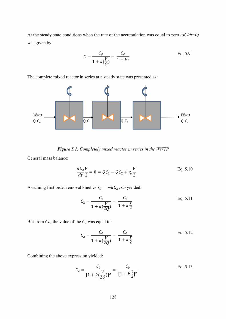
128

At the steady state conditions when the rate of the accumulation was equal to zero (dC/dt=0)

was given by:

𝐶𝐶 =𝐶𝐶𝑂𝑂

1 + 𝑘𝑘(𝑉𝑉𝑄𝑄)=

𝐶𝐶𝑂𝑂1 + 𝑘𝑘𝜏𝜏

Eq. 5.9

The complete mixed reactor in series at a steady state was presented as:

Figure 5.1: Completely mixed reactor in series in the WWTP

General mass balance:

𝑑𝑑𝐶𝐶2𝑑𝑑𝑡𝑡

𝑉𝑉2

= 0 = 𝑄𝑄𝐶𝐶1 − 𝑄𝑄𝐶𝐶2 + 𝑟𝑟𝑣𝑣𝑉𝑉2

Eq. 5.10

Assuming first order removal kinetics 𝑟𝑟𝐶𝐶 = −𝑘𝑘𝐶𝐶2 , C2 yielded:

𝐶𝐶2 =𝐶𝐶1

1 + 𝑘𝑘( 𝑉𝑉2𝑄𝑄)=

𝐶𝐶11 + 𝑘𝑘 𝜏𝜏2

Eq. 5.11

But from Co, the value of the C1 was equal to:


1 + 𝑘𝑘( 𝑉𝑉2𝑄𝑄)=

𝐶𝐶01 + 𝑘𝑘 𝜏𝜏2

Eq. 5.12

Combining the above expression yielded:


[1 + 𝑘𝑘( 𝑉𝑉2𝑄𝑄)]2=

𝐶𝐶0[1 + 𝑘𝑘 𝜏𝜏2]2

Eq. 5.13

Influent EffluentQ, Co Q, C1 Q, C2 Q, Cn

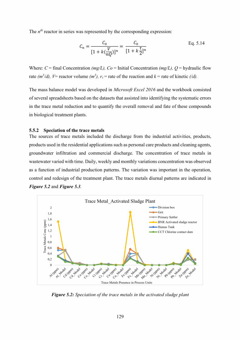
129

The nth reactor in series was represented by the corresponding expression:

𝐶𝐶𝑛𝑛 =𝐶𝐶0

[1 + 𝑘𝑘( 𝑉𝑉𝑟𝑟𝑄𝑄)]𝑛𝑛=

𝐶𝐶0[1 + 𝑘𝑘 𝜏𝜏2]𝑛𝑛

Eq. 5.14

Where: C = final Concentration (mg/L), Co = Initial Concentration (mg/L), Q = hydraulic flow

rate (m3/d), V= reactor volume (m3), rc = rate of the reaction and k = rate of kinetic (/d).

The mass balance model was developed in Microsoft Excel 2016 and the workbook consisted

of several spreadsheets based on the datasets that assisted into identifying the systematic errors

in the trace metal reduction and to quantify the overall removal and fate of these compounds

in biological treatment plants.

5.5.2 Speciation of the trace metals The sources of trace metals included the discharge from the industrial activities, products,

products used in the residential applications such as personal care products and cleaning agents,

groundwater infiltration and commercial discharge. The concentration of trace metals in

wastewater varied with time. Daily, weekly and monthly variations concentration was observed

as a function of industrial production patterns. The variation was important in the operation,

control and redesign of the treatment plant. The trace metals diurnal patterns are indicated in

Figure 5.2 and Figure 5.3.

Figure 5.2: Speciation of the trace metals in the activated sludge plant

0

0,2

0,4

0,6

0,8

1

1,2

1,4

1,6

1,8

2

Trac

e M

etal

s Con

c (p

pm)

Trace Metals Presence in Process Units

Trace Metal_Activated Sludge PlantDivision boxGritPrimary SettlerBNR Activated sludge reactorHumas TankCCT Chlorine contact dam

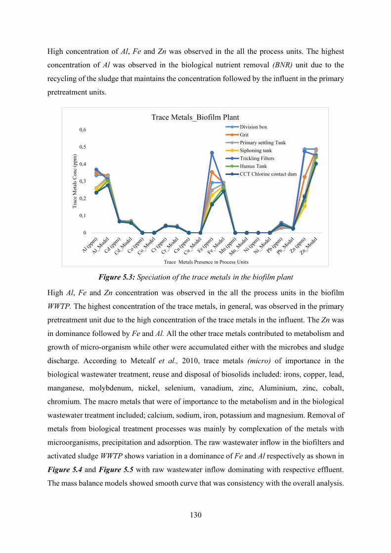
130

High concentration of Al, Fe and Zn was observed in the all the process units. The highest

concentration of Al was observed in the biological nutrient removal (BNR) unit due to the

recycling of the sludge that maintains the concentration followed by the influent in the primary

pretreatment units.

Figure 5.3: Speciation of the trace metals in the biofilm plant

High Al, Fe and Zn concentration was observed in the all the process units in the biofilm

WWTP. The highest concentration of the trace metals, in general, was observed in the primary

pretreatment unit due to the high concentration of the trace metals in the influent. The Zn was

in dominance followed by Fe and Al. All the other trace metals contributed to metabolism and

growth of micro-organism while other were accumulated either with the microbes and sludge

discharge. According to Metcalf et al., 2010, trace metals (micro) of importance in the

biological wastewater treatment, reuse and disposal of biosolids included: irons, copper, lead,

manganese, molybdenum, nickel, selenium, vanadium, zinc, Aluminium, zinc, cobalt,

chromium. The macro metals that were of importance to the metabolism and in the biological

wastewater treatment included; calcium, sodium, iron, potassium and magnesium. Removal of

metals from biological treatment processes was mainly by complexation of the metals with

microorganisms, precipitation and adsorption. The raw wastewater inflow in the biofilters and

activated sludge WWTP shows variation in a dominance of Fe and Al respectively as shown in

Figure 5.4 and Figure 5.5 with raw wastewater inflow dominating with respective effluent.

The mass balance models showed smooth curve that was consistency with the overall analysis.

0

0,1

0,2

0,3

0,4

0,5

0,6

Trac

e M

etal

s Con

c (p

pm)

Trace Metals Presence in Process Units

Trace Metals_Biofilm PlantDivision boxGritPrimary settling TankSiphoning tankTrickling FiltersHumas TankCCT Chlorine contact dam

131

Mass balance model allowed detection of inconsistencies within the trace metals datasets and

assisted in identifying the systematic errors in the metal reduction.

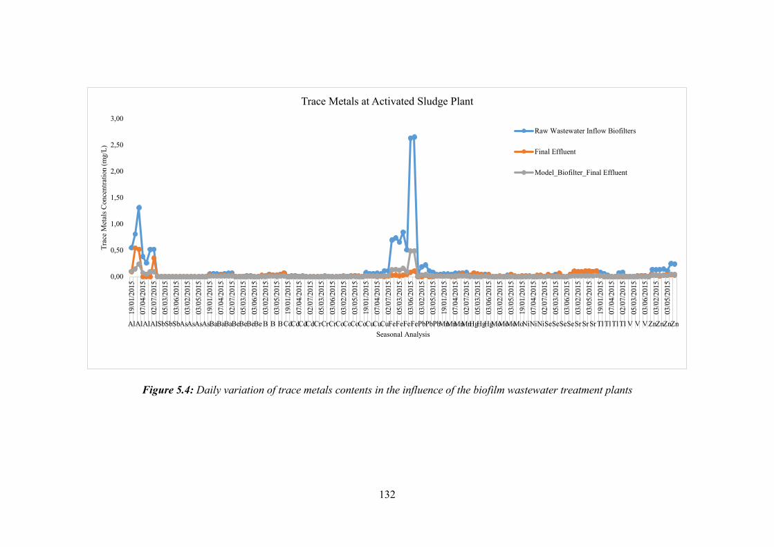
132

Figure 5.4: Daily variation of trace metals contents in the influence of the biofilm wastewater treatment plants

0,00

0,50

1,00

1,50

2,00

2,50

3,00

19/0

1/20

1507

/04/

2015

02/0

7/20

1505

/03/

2015

03/0

6/20

1503

/02/

2015

03/0

5/20

1519

/01/

2015

07/0

4/20

1502

/07/

2015

05/0

3/20

1503

/06/

2015

03/0

2/20

1503

/05/

2015

19/0

1/20

1507

/04/

2015

02/0

7/20

1505

/03/

2015

03/0

6/20

1503

/02/

2015

03/0

5/20

1519

/01/

2015

07/0

4/20

1502

/07/

2015

05/0

3/20

1503

/06/

2015

03/0

2/20

1503

/05/

2015

19/0

1/20

1507

/04/

2015

02/0

7/20

1505

/03/

2015

03/0

6/20

1503

/02/

2015

03/0

5/20

1519

/01/

2015

07/0

4/20

1502

/07/

2015

05/0

3/20

1503

/06/

2015

03/0

2/20

1503

/05/

2015

19/0

1/20

1507

/04/

2015

02/0

7/20

1505

/03/

2015

03/0

6/20

1503

/02/

2015

03/0

5/20

15

AlAlAlAlSbSbSbAsAsAsAsBaBaBaBeBeBeBe B B BCdCdCdCdCrCrCrCoCoCoCoCuCuCuFeFeFeFePbPbPbMnMnMnMnHgHgHgMoMoMoMoNiNiNiSeSeSeSeSrSrSrTlTlTlTl V V VZnZnZnZn

Trac

e M

etal

s Con

cent

ratio

n (m

g/L)

Seasonal Analysis

Trace Metals at Activated Sludge Plant

Raw Wastewater Inflow Biofilters

Final Effluent

Model_Biofilter_Final Effluent

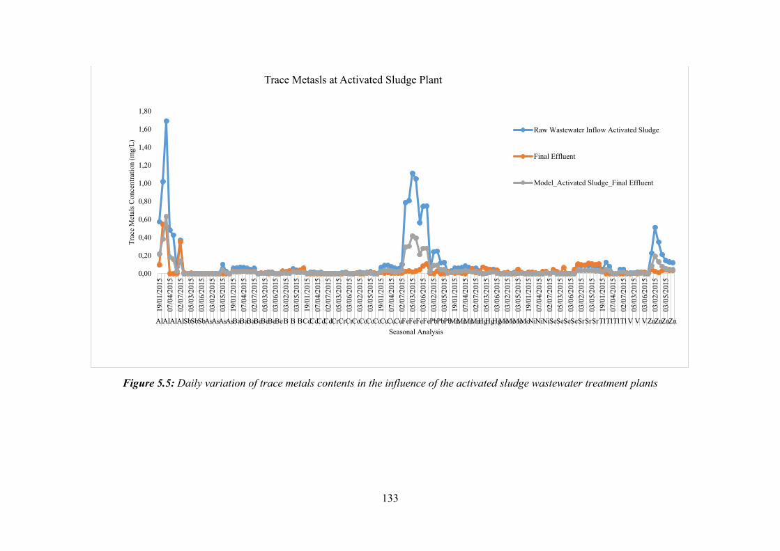
133

Figure 5.5: Daily variation of trace metals contents in the influence of the activated sludge wastewater treatment plants

0,00

0,20

0,40

0,60

0,80

1,00

1,20

1,40

1,60

1,80

19/0

1/20

1507

/04/

2015

02/0

7/20

1505

/03/

2015

03/0

6/20

1503

/02/

2015

03/0

5/20

1519

/01/

2015

07/0

4/20

1502

/07/

2015

05/0

3/20

1503

/06/

2015

03/0

2/20

1503

/05/

2015

19/0

1/20

1507

/04/

2015

02/0

7/20

1505

/03/

2015

03/0

6/20

1503

/02/

2015

03/0

5/20

1519

/01/

2015

07/0

4/20

1502

/07/

2015

05/0

3/20

1503

/06/

2015

03/0

2/20

1503

/05/

2015

19/0

1/20

1507

/04/

2015

02/0

7/20

1505

/03/

2015

03/0

6/20

1503

/02/

2015

03/0

5/20

1519

/01/

2015

07/0

4/20

1502

/07/

2015

05/0

3/20

1503

/06/

2015

03/0

2/20

1503

/05/

2015

19/0

1/20

1507

/04/

2015

02/0

7/20

1505

/03/

2015

03/0

6/20

1503

/02/

2015

03/0

5/20

15

AlAlAlAlSbSbSbAsAsAsAsBaBaBaBeBeBeBeB B BCdCdCdCdCrCrCrCoCoCoCoCuCuCuFeFeFeFePbPbPbMnMnMnMnHgHgHgMoMoMoMoNiNiNiSeSeSeSeSrSrSrTlTlTlTl V V VZnZnZnZn

Trac

e M

etal

s Con

cent

ratio

n (m

g/L)

Seasonal Analysis

Trace Metasls at Activated Sludge Plant

Raw Wastewater Inflow Activated Sludge

Final Effluent

Model_Activated Sludge_Final Effluent

134

All the treatment plants showed a distinctly marked profile with a high concentration of trace

metals independence of the high load. The trace metals in the wastewater could influence the

possibilities for reuse of the wastewater treatment sludge to the agriculture sector by providing

the nutrients to the soil. Trace metals in wastewater have a benefactor in metabolism, the

growth of biological life and absence of sufficient quantities that lead to micro-pollution,

toxicity and limit the growth of algae. According to Metcalf et al., 2010, microbes combine

with metals ions and negatively discharge to the surface. The precipitation works under

addition of chlorides for the formation of metal sulfides in anaerobic digestion. Trace metals

are said to be complexed by carboxyl group found in microbial polysaccharides and other

polymers or absorbed by protein materials in the biological cells (Metcalf et al., 2010).

According to Mullen et al. (1989) and Ahluwalia & Goyal (2007) Freundlich isotherm models,

the removal of metals in biological processes were found to fit into the adsorption

characteristics. All the trace metals were below the threshold 20 mg/L and compiled with the

wastewater treatment plant license and international standards (see Appendix D) (Abdel-Shafy

& Mansour, 2014; Department of Water and Sanitation, [Accessed June 2016]; Mackenzie,

2011; Raval et al., 2016). According to Pomiès et al. (2013), the removal efficiency depends

on physio-chemical of the trace metals, WWTP operating conditions (parameters), hydraulic

retention time (HRT), sludge retention time (SRT) and temperature. Another study by Luo et

al., 2014 suggested regardless of the technology employed, the trace metal removal depends

on physio-chemical properties of the micropollutants and the treatment conditions, and it is

essential for the effectively predicting of the impact on the receiving environment.

5.6 Conclusion

The effective operation of wastewater treatment plants played an important role in

minimalizing the release of trace metals into the aquatic environment. The predicted fate of

transport of the trace metals in the wastewater treatment plant was modelled using mass balance

concept. This show a speciation of the trace metals in multiple units associated with water, air,

microbes, biosolids and biomass, with biological treatment systems with the quantitative

dependent upon physical-chemical and biological properties. Using the mass balance model

made the integrated design process friendly and easier especially in data-entry and making

results of the analysis process easy and understandable. The mass balance showed removal

performance and treatment efficiency of the wastewater treatment plant.

135

CHAPTER 6: AI-BASED BASED PREDICTION MODEL FOR TRACE METALS AND

COD IN THE WASTEWATER TREATMENT USING ARTIFICIAL NEURAL NETWORKS

6.1 Summary

Artificial intelligence (AI) applications are finding their ways into the mainstream lifestyles in

our day to day operations. Novel AI application techniques such as the artificial neural network

(ANN), expert systems (ES), fuzzy logic (FL) and genetic algorithms (GA) have gain popularity

and space program in the fourth industrial revolution (FIR). The goal of the wastewater

treatment process is the reduction of the level of pollutants prior to discharge to the

environment. The interrelationship between COD and pH was studied using AI-based

prediction model (data-driven modelling) with ANNs (universal approximators) incorporated

in MATLAB (neural network toolbox). Supervised learning algorithm was adopted for training

the ANNs and to relate input data to output data. The appropriate architecture of the ANNs was

determined using several steps of training and testing of the models. The training aimed at

estimating, validating, predicting the parameters by an error function minimization. The ANN

model provided accurate predictions of the effluent stream, in terms of COD and trace metals

speciation. The goodness of the prediction (prediction performance) was attained with the

coefficient of determination (R2) of 0.98-0.99, sum of square error (SSE) 0.00029-0.1598, room

mean-square error (RMSE) of 0.0049-0.8673, mean squared error (MSE) 2.7059e-14 to

2.3175e-15. The ANN-based models were found to be a robust tool for predicting WWTP

performance. This revealed that the influent indices could be applied to the prediction of the

effluent quality (EQ). The approach can also be used to handle many other types of waste

treatment plants, environmental management, and emerging technologies so as to meet the

cost-effectiveness, environmental, technical criteria and wide range of big data support in the

implementation of the sustainable development goals (SDGs).

6.2 Introduction

The increasing rhythm of urbanization, industrialization, and population increase has created

uncertainty on the environmental problems with the uncertainty of knowledge and multiplicity

of scales in the FIR (Poch, Comas, Rodríguez, Sanchez & Cortés, 2004). Improper maintenance

136

of wastewater treatment plant (WWTP), the wide range of operating conditions, can trigger

serious public health problem and ecological that affects the flora and fauna (Manu & Thalla,

2017). Due to complex interactions between biological reaction mechanisms, physical,

chemical reaction, kinetics, catalysis, separation, transport phenomena, emerging

micropollutants, multi-variables aspects of the wastewater treatment process, highly non-

linear, highly time-varying, the diagnosis of the WWTP practice, heterogeneity,

incompleteness, and imprecision of the WWTP’s data, etc. makes WWTP to have a unique

characteristic as compared to other environmental and biotechnological industrial processes

(Hong, Rosen & Bhamidimarri, 2003; Poch et al., 2004; Zeng et al., 2003). The biological

WWTP often receive variation in raw wastewater composition that can pose substantial quality

environmental imbalance and a high cost of operation if not well control and predicted, strength

and flow rates because of the complex nature of the treatment process (Belanche, Valdés,

Comas, Roda & Poch, 1999; Nasr, Moustafa, Seif & El Kobrosy, 2012; Qing, Wang & Meng,

2005). Missing data (datasets) due to error handling systems, has been reported to affect the

learning and classification accuracies in data analysis, prediction and modelling (Duma,

Marwala, Twala & Nelwamondo, 2013). The successful management of these systems requires

multidisciplinary approaches from different engineering, big data, AI, machine learning (ML),

deep learning (DL), data science, data mining, advanced analytics, automation, blockchain

technology, biotechnology, microbiology, data streaming, social science and other scientific

fields. AI techniques (data-driven modeling) have been used in different sectors such as

engineering, marine, economics, meteorological, remote sensing, medicine, military, etc. to

prediction, forecasting, optimization, modeling, identification, and control of complex systems

in the quest of implementing and achieving the sustainable development goals (Mellit &

Kalogirou, 2008).

The application of the artificial intelligence using multi-dimensional process datasets,

visualization techniques can be applied to the prediction and forecast of the WWTP (Hong et

al., 2003). The complexity of environmental problems makes it necessary to develop and apply

to new tools capable of processing data and decision-making processes using tools like

environmental decision support systems (EDSSs). EDSS can integrate the AI techniques,

geographical information systems (GIS), statistical/numerical methods and environmental

tautologies (Poch et al., 2004; Rizzoli & Young, 1997). It is difficult to make most

environmental, economic, technical, social and ecological decision without careful forecasting,

prediction, modelling and analysis of the development scenarios. This enables the management

137

and stakeholders to choose an option that satisfies a large number of identified conditions and

taking into consideration the precaution measure in advance (Palani, Liong & Tkalich, 2008).

Various control actions have to be implemented for efficient monitoring of process performed

during the operation of WWTP (Manu & Thalla, 2017). Most WWTP designs are based on

waste resources and energy, crisis conditions, and reduce the cost-effectiveness of reaching

permissible effluent levels (Wen & Vassiliadis, 1998). The engineers and scientist have

extensive experience on the process-based model and data-driven techniques like artificial

intelligence with deep learning/machine learning. Process-based models can provide good

estimations of the wastewater process parameters or variables but require approximation and

estimation of the process variables and lengthy data calibration process. Process-based models

require a lot of the input data and a large number of specification model parameters that are

unknown unlike the data-driven model techniques that are computational fast, and requires

fewer inputs parameters and thus provides alternative to the process-based model (Hong et al.,

2003; Palani et al., 2008).

6.3 Hybrid AI Techniques

Artificial intelligent models application tools such as artificial neural network (ANN), fuzzy

logic (FL), expert systems (ES), support vector machine (SVM), neuro-fuzzy inference systems

(ANFIS), knowledge-based systems (KBS), fuzzy logic control (FLC), pattern recognition

(PR), case-based systems (CBS), ruled-based reasoning (RBR), ruled based systems (RBS),

swarm intelligence (SI), reinforcement learning (RL), hybrid systems (HS), expert systems (ES)

and genetic algorithms (GA) have gain popularity and space program in the fourth industrial

revolution (Chen, Jakeman & Norton, 2008; Choi & Park, 2001; Dellana & West, 2009; Pai et

al., 2009; Poch et al., 2004; Wen & Vassiliadis, 1998). Global development of supervision

tools and reliable real-time control was applied to wastewater treatment process. ANN has

proven to be the universal tool for forecasting and prediction where the desired input-output

transformation is usually determined by external, supervised adjustment of the system

parameters (Hong et al., 2003). ANNs are designed to solve the type of problems where the

outputs are required are unknown (unsupervised learning algorithms) and known output

(supervised learning algorithms) (Hong et al., 2003). The basic structures of an ANN are: (1)

input layer where data are introduced to the model and computational of the weighted sum of

the input is performed, (b) the hidden layer(s) where the data are processed and lastly, (3)

output layer, where the results of the ANN are produced (Singh, Basant, Malik & Jain, 2009).

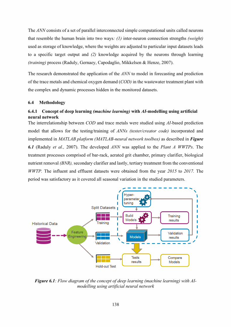
138

The ANN consists of a set of parallel interconnected simple computational units called neurons

that resemble the human brain into two ways: (1) inter-neuron connection strengths (weight)

used as storage of knowledge, where the weights are adjusted to particular input datasets leads

to a specific target output and (2) knowledge acquired by the neurons through learning

(training) process (Raduly, Gernaey, Capodaglio, Mikkelsen & Henze, 2007).

The research demonstrated the application of the ANN to model in forecasting and prediction

of the trace metals and chemical oxygen demand (COD) in the wastewater treatment plant with

the complex and dynamic processes hidden in the monitored datasets.

6.4 Methodology

6.4.1 Concept of deep learning (machine learning) with AI-modelling using artificial neural network The interrelationship between COD and trace metals were studied using AI-based prediction

model that allows for the testing/training of ANNs (tester/creator code) incorporated and

implemented in MATLAB platform (MATLAB-neural network toolbox) as described in Figure

6.1 (Raduly et al., 2007). The developed ANN was applied to the Plant A WWTPs. The

treatment processes comprised of bar-rack, aerated grit chamber, primary clarifier, biological

nutrient removal (BNR), secondary clarifier and lastly, tertiary treatment from the conventional

WWTP. The influent and effluent datasets were obtained from the year 2015 to 2017. The

period was satisfactory as it covered all seasonal variation in the studied parameters.

Figure 6.1: Flow diagram of the concept of deep learning (machine learning) with AI-modelling using artificial neural network

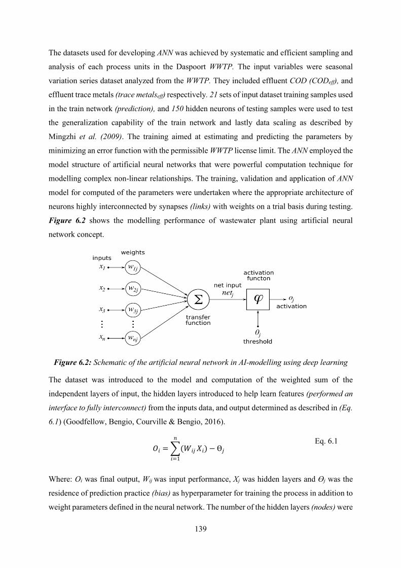
139

The datasets used for developing ANN was achieved by systematic and efficient sampling and

analysis of each process units in the Daspoort WWTP. The input variables were seasonal

variation series dataset analyzed from the WWTP. They included effluent COD (CODeff), and

effluent trace metals (trace metalseff) respectively. 21 sets of input dataset training samples used

in the train network (prediction), and 150 hidden neurons of testing samples were used to test

the generalization capability of the train network and lastly data scaling as described by

Mingzhi et al. (2009). The training aimed at estimating and predicting the parameters by

minimizing an error function with the permissible WWTP license limit. The ANN employed the

model structure of artificial neural networks that were powerful computation technique for

modelling complex non-linear relationships. The training, validation and application of ANN

model for computed of the parameters were undertaken where the appropriate architecture of

neurons highly interconnected by synapses (links) with weights on a trial basis during testing.

Figure 6.2 shows the modelling performance of wastewater plant using artificial neural

network concept.

Figure 6.2: Schematic of the artificial neural network in AI-modelling using deep learning

The dataset was introduced to the model and computation of the weighted sum of the

independent layers of input, the hidden layers introduced to help learn features (performed an

interface to fully interconnect) from the inputs data, and output determined as described in (Eq.

6.1) (Goodfellow, Bengio, Courville & Bengio, 2016).

𝑁𝑁𝑟𝑟 = �(𝑊𝑊𝑟𝑟𝑖𝑖

𝑟𝑟

𝑟𝑟=1𝑉𝑉𝑟𝑟)−Ɵ𝑖𝑖

Eq. 6.1

Where: Oi was final output, Wij was input performance, Xj was hidden layers and Ɵj was the

residence of prediction practice (bias) as hyperparameter for training the process in addition to

weight parameters defined in the neural network. The number of the hidden layers (nodes) were

140

determined on trial and error basis with a rule of thumb relied on the fact of the number of

samples in the training set should at least be greater than the number of the synaptic weights.

The node’s output determined using a mathematical operation on the node’s net input with

transfer function operation (sigmoid, hyperbolic tangent, liner transfer function) as (Nasr et

al., 2012):

• Sigmoid transfer function (Eq. 6.2:

𝑜𝑜(𝑜𝑜) =1

1 + 𝑟𝑟−𝑚𝑚 0 ≤ 𝑜𝑜(𝑜𝑜) ≤ 1

Eq. 6.2

• Hyperbolic tangent transfer function (Eq. 6.3:

𝑜𝑜(𝑜𝑜) = 𝑡𝑡𝑟𝑟𝑟𝑟ℎ (𝑜𝑜) =𝑟𝑟𝑚𝑚 − 𝑟𝑟−𝑚𝑚

𝑟𝑟𝑚𝑚 + 𝑟𝑟−𝑚𝑚 − 1 ≤ 𝑜𝑜(𝑜𝑜) ≤ 1

Eq. 6.3

• Linear transfer function (Eq. 6.4

𝑜𝑜(𝑜𝑜) = 𝑜𝑜 −∞ < 𝑜𝑜(𝑜𝑜) < +∞

Eq. 6.4

The train and test data were generated by the probability distribution over datasets called data

generating process. To achieve the machine learning (deep learning) modern practice goals, a

foundational concept such as bias, variance and parameters estimation was useful to formally

characterize the notion of overfitting, underfitting and generalization. The prediction problems,

a supervised learning algorithm was adopted for training the network. The MATLAB opens the

network/data manager window (App Toolbox-Neural Network Fitting Tool-nftool) that allows

the user to import, create, use and export neural networks and data. The networks properties

included: network inputs-COD effluent and trace metals effluent, network output-permissible

effluent limits, network type-feed-forward back propagation, training function-TRAINLM,

adaptation learning function-LEARNGDM, number of hidden layers (neurons)-150 and use of

default Levenberg-Marquardt algorithms for training (Mjalli, Al-Asheh & Alfadala, 2007).

6.4.2 Model performance evaluation This minimized the error (deviation of the forecasting analysis) while the model makes the

perfectly correct prediction in machine training (deep learning). All the computations were

done with Microsoft Excel 2016 and MATLAB (MathWorks, Inc.)-deep learning with

Levenberg-Marquardt algorithms (LMA) for solving generic curve-fitting problems (non-linear

least square problems) (Mathworks, 1994-2018a, 1994-2018b; Ngia & Sjoberg, 2000)

(Mathworks, 2016).

141

The goodness of the prediction (prediction performance) was attained with room mean-square

error (RMSE)-(Eq. 6.5), mean squared error (MSE)-(Eq. 6.6), sum of squared error (SSE)- (Eq.

6.7), coefficient of determination (R2)-(Eq. 6.8) (Mingzhi et al., 2009; Pai et al., 2011; Wan et

al., 2011).

𝑅𝑅𝑀𝑀𝑆𝑆𝐸𝐸 = �1𝑟𝑟�(𝑌𝑌𝑎𝑎 − 𝑌𝑌𝑜𝑜)2𝑛𝑛

𝑡𝑡=1

Eq. 6.5

𝑀𝑀𝑆𝑆𝐸𝐸 = �

(𝑌𝑌𝑎𝑎 − 𝑌𝑌𝑜𝑜)2

𝑟𝑟

𝑛𝑛

𝑡𝑡=2

Eq. 6.6

𝑆𝑆𝑆𝑆𝐸𝐸 = �(𝑌𝑌𝑎𝑎 − 𝑌𝑌𝑜𝑜)2𝑛𝑛

𝑡𝑡=2

Eq. 6.7

𝑅𝑅2 = 1−𝑆𝑆𝑆𝑆𝑅𝑅𝑟𝑟𝑔𝑔𝑟𝑟𝑟𝑟𝑀𝑀𝑀𝑀𝑟𝑟𝑜𝑜𝑟𝑟𝑆𝑆𝑆𝑆𝑅𝑅𝑜𝑜𝑡𝑡𝑟𝑟𝑙𝑙

Eq. 6.8

Where: n is the number of data point/training/test samples, Ya is the target/actual/desired output,

Yo is the network/predict output, SSTotal total summed squared error based on the mean,

SSRegression is the sum of squared error based off the regression line.

6.5 Results and Discussion

6.5.1 Effect of trace metals and chemical oxygen demand in the wastewater treatment process Due to the inherent complexity, chemical composition, incoherent flow rate and higher safety

factor in the effective operation of the biological wastewater treatment process, the AI-based

model was extensively tested in managing the wastewater treatment operations. Modelling was

accomplished with ANN (universal approximator) due to WWTP non-uniformity and non-

linearity of the biological treatment. The plant input and output data were used to predict the

plant without using mechanistic bio-modelling that involves a great degree of complexity and

uncertainty. The effect of the COD and trace metal in the wastewater treatment processes were

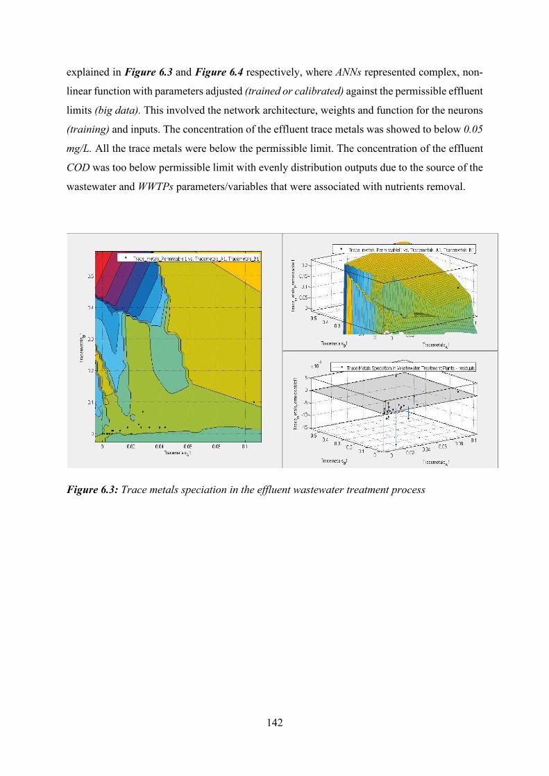
142

explained in Figure 6.3 and Figure 6.4 respectively, where ANNs represented complex, non-

linear function with parameters adjusted (trained or calibrated) against the permissible effluent

limits (big data). This involved the network architecture, weights and function for the neurons

(training) and inputs. The concentration of the effluent trace metals was showed to below 0.05

mg/L. All the trace metals were below the permissible limit. The concentration of the effluent

COD was too below permissible limit with evenly distribution outputs due to the source of the

wastewater and WWTPs parameters/variables that were associated with nutrients removal.

Figure 6.3: Trace metals speciation in the effluent wastewater treatment process

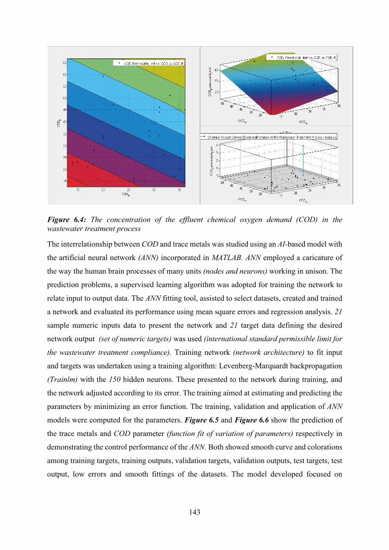
143

Figure 6.4: The concentration of the effluent chemical oxygen demand (COD) in the wastewater treatment process

The interrelationship between COD and trace metals was studied using an AI-based model with

the artificial neural network (ANN) incorporated in MATLAB. ANN employed a caricature of

the way the human brain processes of many units (nodes and neurons) working in unison. The

prediction problems, a supervised learning algorithm was adopted for training the network to

relate input to output data. The ANN fitting tool, assisted to select datasets, created and trained

a network and evaluated its performance using mean square errors and regression analysis. 21

sample numeric inputs data to present the network and 21 target data defining the desired

network output (set of numeric targets) was used (international standard permissible limit for

the wastewater treatment compliance). Training network (network architecture) to fit input

and targets was undertaken using a training algorithm: Levenberg-Marquardt backpropagation

(Trainlm) with the 150 hidden neurons. These presented to the network during training, and

the network adjusted according to its error. The training aimed at estimating and predicting the

parameters by minimizing an error function. The training, validation and application of ANN

models were computed for the parameters. Figure 6.5 and Figure 6.6 show the prediction of

the trace metals and COD parameter (function fit of variation of parameters) respectively in

demonstrating the control performance of the ANN. Both showed smooth curve and colorations

among training targets, training outputs, validation targets, validation outputs, test targets, test

output, low errors and smooth fittings of the datasets. The model developed focused on

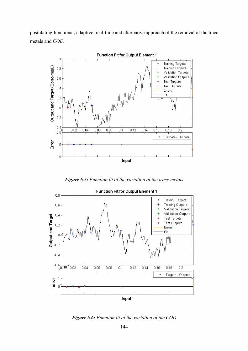
144

postulating functional, adaptive, real-time and alternative approach of the removal of the trace

metals and COD.

Figure 6.5: Function fit of the variation of the trace metals

Figure 6.6: Function fit of the variation of the COD

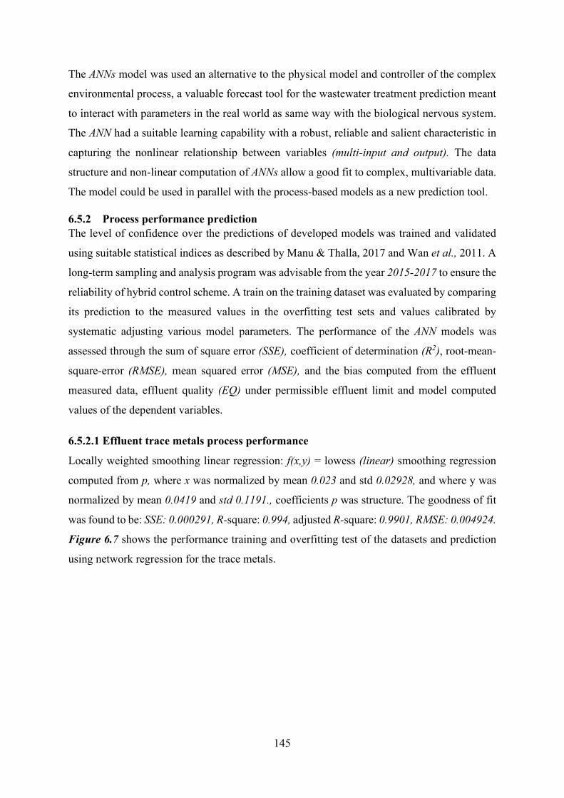
145

The ANNs model was used an alternative to the physical model and controller of the complex

environmental process, a valuable forecast tool for the wastewater treatment prediction meant

to interact with parameters in the real world as same way with the biological nervous system.

The ANN had a suitable learning capability with a robust, reliable and salient characteristic in

capturing the nonlinear relationship between variables (multi-input and output). The data

structure and non-linear computation of ANNs allow a good fit to complex, multivariable data.

The model could be used in parallel with the process-based models as a new prediction tool.

6.5.2 Process performance prediction The level of confidence over the predictions of developed models was trained and validated

using suitable statistical indices as described by Manu & Thalla, 2017 and Wan et al., 2011. A

long-term sampling and analysis program was advisable from the year 2015-2017 to ensure the

reliability of hybrid control scheme. A train on the training dataset was evaluated by comparing

its prediction to the measured values in the overfitting test sets and values calibrated by

systematic adjusting various model parameters. The performance of the ANN models was

assessed through the sum of square error (SSE), coefficient of determination (R2), root-mean-

square-error (RMSE), mean squared error (MSE), and the bias computed from the effluent

measured data, effluent quality (EQ) under permissible effluent limit and model computed

values of the dependent variables.

6.5.2.1 Effluent trace metals process performance

Locally weighted smoothing linear regression: f(x,y) = lowess (linear) smoothing regression

computed from p, where x was normalized by mean 0.023 and std 0.02928, and where y was

normalized by mean 0.0419 and std 0.1191., coefficients p was structure. The goodness of fit

was found to be: SSE: 0.000291, R-square: 0.994, adjusted R-square: 0.9901, RMSE: 0.004924.

Figure 6.7 shows the performance training and overfitting test of the datasets and prediction

using network regression for the trace metals.

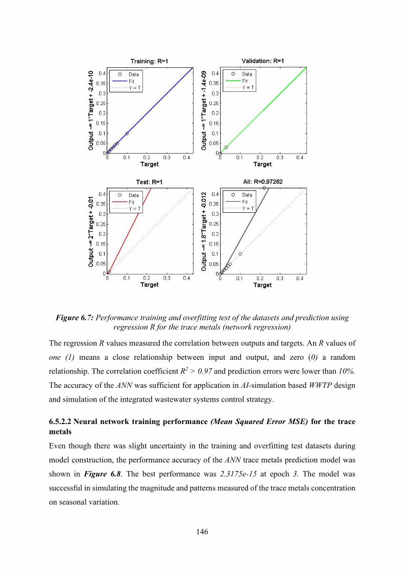
146

Figure 6.7: Performance training and overfitting test of the datasets and prediction using regression R for the trace metals (network regression)

The regression R values measured the correlation between outputs and targets. An R values of

one (1) means a close relationship between input and output, and zero (0) a random

relationship. The correlation coefficient R2 > 0.97 and prediction errors were lower than 10%.

The accuracy of the ANN was sufficient for application in AI-simulation based WWTP design

and simulation of the integrated wastewater systems control strategy.

6.5.2.2 Neural network training performance (Mean Squared Error MSE) for the trace metals

Even though there was slight uncertainty in the training and overfitting test datasets during

model construction, the performance accuracy of the ANN trace metals prediction model was

shown in Figure 6.8. The best performance was 2.3175e-15 at epoch 3. The model was

successful in simulating the magnitude and patterns measured of the trace metals concentration

on seasonal variation.

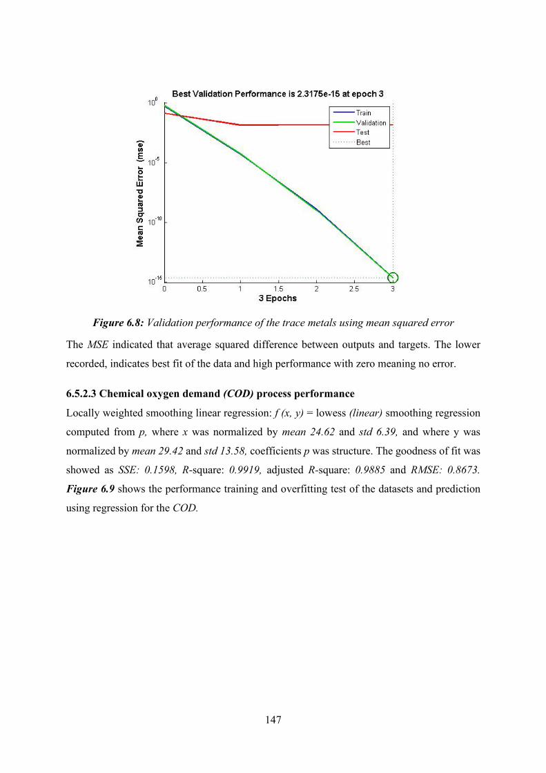
147

Figure 6.8: Validation performance of the trace metals using mean squared error

The MSE indicated that average squared difference between outputs and targets. The lower

recorded, indicates best fit of the data and high performance with zero meaning no error.

6.5.2.3 Chemical oxygen demand (COD) process performance

Locally weighted smoothing linear regression: f (x, y) = lowess (linear) smoothing regression

computed from p, where x was normalized by mean 24.62 and std 6.39, and where y was

normalized by mean 29.42 and std 13.58, coefficients p was structure. The goodness of fit was

showed as SSE: 0.1598, R-square: 0.9919, adjusted R-square: 0.9885 and RMSE: 0.8673.

Figure 6.9 shows the performance training and overfitting test of the datasets and prediction

using regression for the COD.

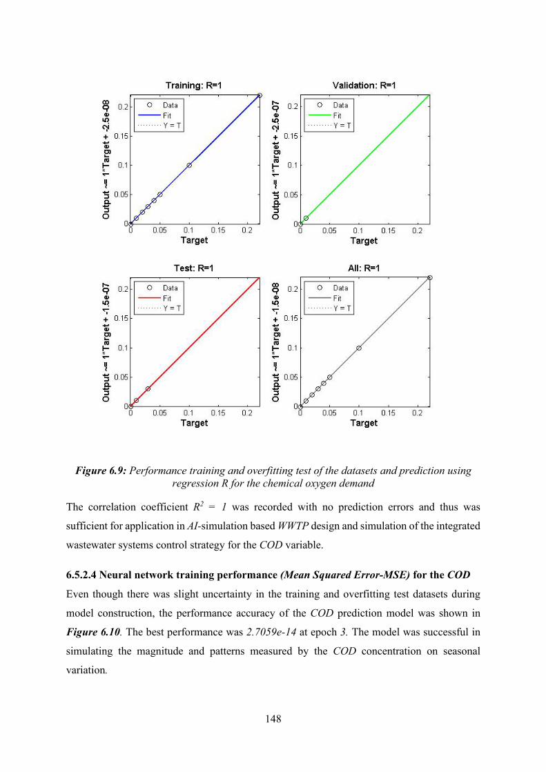
148

Figure 6.9: Performance training and overfitting test of the datasets and prediction using regression R for the chemical oxygen demand

The correlation coefficient R2 = 1 was recorded with no prediction errors and thus was

sufficient for application in AI-simulation based WWTP design and simulation of the integrated

wastewater systems control strategy for the COD variable.

6.5.2.4 Neural network training performance (Mean Squared Error-MSE) for the COD

Even though there was slight uncertainty in the training and overfitting test datasets during

model construction, the performance accuracy of the COD prediction model was shown in

Figure 6.10. The best performance was 2.7059e-14 at epoch 3. The model was successful in

simulating the magnitude and patterns measured by the COD concentration on seasonal

variation.

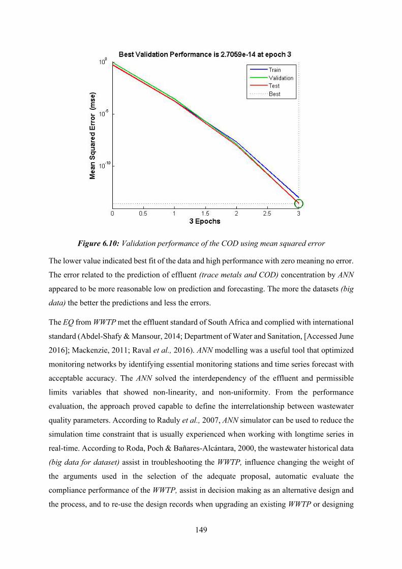
149

Figure 6.10: Validation performance of the COD using mean squared error

The lower value indicated best fit of the data and high performance with zero meaning no error.

The error related to the prediction of effluent (trace metals and COD) concentration by ANN

appeared to be more reasonable low on prediction and forecasting. The more the datasets (big

data) the better the predictions and less the errors.

The EQ from WWTP met the effluent standard of South Africa and complied with international

standard (Abdel-Shafy & Mansour, 2014; Department of Water and Sanitation, [Accessed June

2016]; Mackenzie, 2011; Raval et al., 2016). ANN modelling was a useful tool that optimized

monitoring networks by identifying essential monitoring stations and time series forecast with

acceptable accuracy. The ANN solved the interdependency of the effluent and permissible

limits variables that showed non-linearity, and non-uniformity. From the performance

evaluation, the approach proved capable to define the interrelationship between wastewater

quality parameters. According to Raduly et al., 2007, ANN simulator can be used to reduce the

simulation time constraint that is usually experienced when working with longtime series in

real-time. According to Roda, Poch & Bañares-Alcántara, 2000, the wastewater historical data

(big data for dataset) assist in troubleshooting the WWTP, influence changing the weight of

the arguments used in the selection of the adequate proposal, automatic evaluate the

compliance performance of the WWTP, assist in decision making as an alternative design and

the process, and to re-use the design records when upgrading an existing WWTP or designing

150

a similar WWTP capacity. Deep learning with machine learning in AI-modelling approach

could provide alternatives to a generic framework for the modelling of other treatment

processes.

6.6 Conclusion

The widely used artificial intelligence (AI)-based prediction models ANN, using MATLAB

platform incorporated with machine learning (deep learning) was used to predict the real-life

problems of the wastewater treatment processes. Since there was no need to define complex

reaction, mathematical and biochemical equation in the use of the AI-based models, it was

suggested to conduct the simultaneous machine learning with the most appropriate model

structure for the specific problems. The deep learning, a new area of a set of algorithms in

machine learning principles was efficient and elegant techniques served with a modern

paradigm for computing and simulating biological; and environmental design processes with a

basic principle of the prediction modelling. The efficiency of operating biological wastewater

treatment processes was significantly influenced by an overload in a local community due to

varying wastewater source, flow rate and chemical composition. The results presented

confirmed that ANNs as a good tool for the simulation model of the WWTP designs and

development of the integrated wastewater systems. The limited time used to train big data

(datasets) allows faster performance evaluation as compared to conventional modelling. The

ANN was useful in solving data-intensive problems where algorithm or rules to solve the

problem was limited/unknown/difficult to express and can be used as the objective function or

constraints in optimization for the best operation or design in the future studies. The goodness

of the prediction (prediction performance) was attained with the coefficient of determination

(R2) of 0.98-0.99, sum of square error (SSE) 0.00029-0.1598, room mean-square error (RMSE)

of 0.0049-0.8673, mean squared error (MSE) 2.7059e-14 to 2.3175e-15 for the trace metals and

COD concentration respectively. The prediction accuracy of the ANN was sufficient for the

applications envisaged in the simulation of the non-linear behaviour of the plant and valuable

performance assessment tool for WWTP operations and decision making in troubleshooting. It

revealed that the influent indices could be applied to the prediction of the effluent quality.

151

CHAPTER 7: CONCLUSIONS AND RECOMMENDATIONS

7.1 Conclusions

Wastewater treatment process can be considered as the largest industry in terms of waste

management industries. The biological behavior of biotechnological processes occurring in a

bioreactor has a complexity unparalleled in the chemistry application principles. The complex

systems therefore result in involvement of the models based on mathematical description of

the process after the off-line sampling and analysis due to lack of the on-line sensor. The study

applied practical knowledge of IAWQ Activated Sludge Model No.1 and mass balance through

a database that combines experience from expert knowledge and modelling experience. The

basis for the development of reliable mathematical models was a thorough understanding of

the process involved. Activated sludge systems was described by mathematical models based

on mass balance equations that relate to change of the state variables of the system (flow rates,

concentration and composition) due to transport and the transformation mechanisms. The

authors combine the ASM1 principles, substrate and microorganisms’ kinetics in mass balance,

thus resulting in a standardized methodology for expressing nomenclature that is useful for the

WWTP modelers and other experts. This will enhance coding in programming of the simulation

software by eliminating error-prone part of model implementation. The spreadsheet provided

corrected matrices with all stoichiometric coefficient for the bio-kinetic models. The presence

of emerging micro-pollutants such as methyparabens, ethylparabens, propylparabens and the

inclusion of water chemistry indicated that the plant has the capability and is effective in

removing the fate of micro-pollutants. COD mass balance made a lot of sense on prediction of

the experimental data that was reliable and accurate. Monitoring the reactor concentration and

its changes at a fixed parameter created a long-term change in the loading rate on the WWTP

and thus increase its efficiency. The structured framework of the models was useful among

modellers, operators and management at the WWTPs and other wastewater stakeholders. The

models provided guidance in identifying the key design parameters and quantify system

parameters that ensured optimal performance. The information provided an insight into the

wastewater characteristic that included biodegradability, flow distribution, contaminants and

potential for the source control. These models provided the quantitative predictions of quality

of effluent to be expected from the design of the existing WWTP and guidance to the direct

attention needed in the system and control response. Use of the ASM1 facilitated

communication of the complex models and enabled a focus on the bio-kinetics models. Mass

152

balance was a powerful tool that allowed detection of inconsistencies within the WWTP data

sets and assisted to identify the systematic errors. The models were verified by conforming to

internal mass balance and adequate validation against the experimental tests. The results

contributed to the knowledge transfer on activated sludge and biofilm modelling. No alarm was

raised from the Daspoort WWTP data analysis efficiency performance and thus the plant met

regulatory targets (permissible effluent limits).

The effective operation of wastewater treatment plants played an important role in

minimalizing the release of trace metals into the aquatic environment. The predicted fate of

transport of the trace metals in the wastewater treatment plant was modelled using mass balance

concept. This show a speciation of the trace metals in multiple units associated with water, air,

microbes, biosolids and biomass, with biological treatment systems with the quantitative

dependent upon physical-chemical and biological properties. Using the mass balance model

made the integrated design process friendly and easier especially for data-entry and the ease of

understanding results of the analysis process. The mass balance showed removal performance

and treatment efficiency of the wastewater treatment plant.

The widely-used artificial intelligence/machine learning/deep learning-based prediction

models ANN, using MATLAB platform was used to predict the real-life problems of the

wastewater treatment processes. Since there was no need to define complex reaction,

mathematical and biochemical equation in the use of the AI-based models, it was suggested to

conduct the simultaneous machine learning with the most appropriate model structure for the

specific problems. The deep learning, a new area of a set of algorithms in machine learning

principles, was efficient and elegant techniques served with a modern paradigm for computing

and simulating biological and environmental design processes with a basic principle of the

prediction modelling. The efficiency of operating biological wastewater treatment processes

was significantly influenced by an overload in a local community due to varying wastewater

source, flow rate and chemical composition. The results presented confirmed ANNs as a good

tool for the simulation model of the WWTP designs and development of the integrated

wastewater systems. The limited time used to train big data (datasets) allows faster

performance evaluation as compared to conventional modelling. The ANN was useful in

solving data-intensive problems where algorithm or rules to solve the problem was

limited/unknown/difficult to express and can be used as the objective function or constraints in

optimization for the best operation or design in the future studies. The goodness of the

153

prediction (prediction performance) was attained with coefficient of determination (R2) of

0.98-0.99, sum of square error (SSE) 0.00029-0.1598, room mean-square error (RMSE) of

0.0049-0.8673 and mean squared error (MSE) 2.7059e-14 to 2.3175e-15 for the trace metals

and COD concentration respectively. The prediction accuracy of the ANN was sufficient for

the applications envisaged in the simulation of the non-linear behavior of the plant and valuable

performance assessment tool for WWTP operations and decision-making in troubleshooting. It

revealed that the influent indices could be applied to the prediction of the effluent quality. The

mathematical modelling study developed an effective design for wastewater treatment plant

process.

7.2 Recommendations

The initial objectives of this project were as follows:

i. To carry out site reconnaissance and dimension of the WWTPs process unit. This was

to assist in getting the complete picture (mass balance) about the occurrence, concentration,

fate and transport of trace metals, organic and inorganic compounds.

ii. To carry out in-depth sampling at different intervals (process units) based on retention

time from the liquid, mixed sludge, dewatered sludge and analyze organics, inorganics, trace

metals and emerging micropollutants.

iii. To analyse thermodynamic and reaction bio-kinetics models that will be used to gain a

better understanding of the variable dependency in the wastewater treatment process, biosolids

utilization.

iv. To carry out mathematical modelling and simulation of the trace metals, organic,

inorganic, micropollutant compounds, physically measured data (operation variables),

performance variables in the WWTPs. This will enable a better understanding of each treatment

unit and henceforth improved analytical strategies for the pollutant’s removal.

v. To optimize parameters and validate empirical results through goodness of the

prediction (prediction performance) to ascertain comparability of satisfactory results.

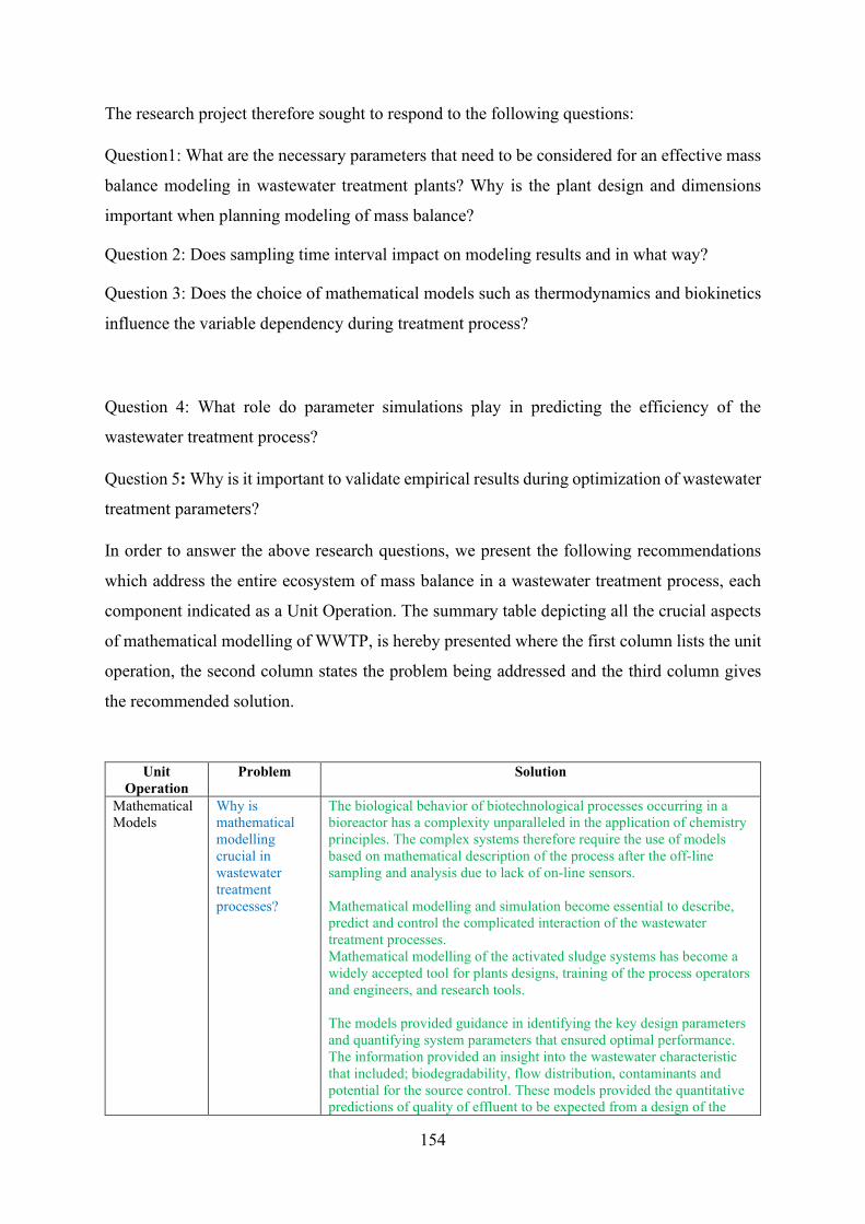
154

The research project therefore sought to respond to the following questions:

Question1: What are the necessary parameters that need to be considered for an effective mass

balance modeling in wastewater treatment plants? Why is the plant design and dimensions

important when planning modeling of mass balance?

Question 2: Does sampling time interval impact on modeling results and in what way?

Question 3: Does the choice of mathematical models such as thermodynamics and biokinetics

influence the variable dependency during treatment process?

Question 4: What role do parameter simulations play in predicting the efficiency of the

wastewater treatment process?

Question 5: Why is it important to validate empirical results during optimization of wastewater

treatment parameters?

In order to answer the above research questions, we present the following recommendations

which address the entire ecosystem of mass balance in a wastewater treatment process, each

component indicated as a Unit Operation. The summary table depicting all the crucial aspects

of mathematical modelling of WWTP, is hereby presented where the first column lists the unit

operation, the second column states the problem being addressed and the third column gives

the recommended solution.

Unit Operation

Problem Solution

Mathematical Models

Why is mathematical modelling crucial in wastewater treatment processes?

The biological behavior of biotechnological processes occurring in a bioreactor has a complexity unparalleled in the application of chemistry principles. The complex systems therefore require the use of models based on mathematical description of the process after the off-line sampling and analysis due to lack of on-line sensors. Mathematical modelling and simulation become essential to describe, predict and control the complicated interaction of the wastewater treatment processes. Mathematical modelling of the activated sludge systems has become a widely accepted tool for plants designs, training of the process operators and engineers, and research tools. The models provided guidance in identifying the key design parameters and quantifying system parameters that ensured optimal performance. The information provided an insight into the wastewater characteristic that included; biodegradability, flow distribution, contaminants and potential for the source control. These models provided the quantitative predictions of quality of effluent to be expected from a design of the

155

existing WWTP and guidance to the direct attention needed in the system and control response.

Control of the process parameters (concentration, flowrates and composition) in terms of real-time

How does population growth globally, economic development, urbanization impact on wastewater treatment processes?

The global population growth, economic development, urbanization, improvement in living-standards has increased waste generation and introduced emerging contaminants into waste streams that may pose sanitary and environmental risks. These contaminants have increased the demand for new approaches to addressing emerging pollutant removals in wastewater. Therefore, to handle smart wastewater treatment processes, instrumentation, control and automation (ICA) is the best approach to enhancing the efficiency of wastewater treatment process. Achieving these process control standards requires the programmable biochemical quantitative-characterization analysis of given waste streams, implementation of innovative integrated waste management systems and reliable waste management data which provides an all-inclusive resource for a comprehensive, critical and informative evaluation of waste management options in waste management programmes. This is due to complex biological reaction mechanisms, lack of reliable on-line instrumentation, unforeseen changes in microbes, organic and inorganic compounds, multivariable aspects of the real wastewater treatment plant (WWTP) and highly time-varying process variables that create a need for the intelligent technique for analysis of multi-dimensional process data known as the ‘big data’ and diagnoses of inter-relationship of the process variables in the WWTPs. This reveal that the influent indices could be applied to the prediction of the effluent quality (EQ). The approach can also be used to handle many other types of waste treatment systems, environmental management, carbon capture and emerging technologies so as to meet the cost-effectiveness, environmental, technical criteria and wide range of big data support in the implementation of the national and sustainable development goals (SDGs).

Impact of primary settlement sizing and velocity

Do carbon, nitrogen and phosphorous elements in the primary sedimentation processes have an impact on the primary sedimentation

The quantity and quality of carbon, nitrogen and phosphorus are much affected by primary settling tank due to sludge discharge before the activated sludge reactor. It is important that the primary sedimentation on the wastewater C, N, and P be determined to enable the settled sewage characterization to be estimated. Sedimentation is characterized by particles that settle discretely at a constant settling velocity and individual particles (sand and grits) do not flocculate during settling. High settling velocity give the high efficiency of the wastewater treatment.

Change of design flowrate (loading) with the hydraulic retention time

How does sludge age affect the efficiency of wastewater treatment?

The hydraulic control of sludge age revolves a greater responsibility to plant operators and in the redesign of the biological processes to improve effluent quality. This can create a pathogen-free effluent. The dynamics created by the daily flow rate of the inflow could be tapped with the installation of the whirlpool turbines to provide power to run the operations of the WWTP and at the same time supply electricity to the local communities.

Effect of the solid retention time in the WWTP

What considerations does one need to take into

The following plant parameters must be considered in the design of the plant: solid retention time (SRT), cell residence time (Ɵ) or sludge age, net specific bacteria growth rate (µnet) and effluent concentration (S) of the biomass

156

account when determining the rate of sedimentation of particles in wastewater?

The SRT could be controlled by the wasting rate a given percentage of the aeration tank volume on each day. Controlling the SRT by sludge wasting affects the net specific biomass growth rate and the reactor substrate concentration. The SRT helped control the sludge age and the underflow and overflow. The wasting of solids is required to prevent an accumulation of solids in the oxidation ditch. It is essential that the designer consider the sludge mass more exactly to provide sufficient reactor volume under design organic load that allowed proper concentration at the specified process unit. The increased in COD mass load increased the sludge concentration automatically and maintained the sludge age. Maintaining the COD mass load constant automatically maintained the sludge concentration constant.

Effect of temperature on microbial growth

What is the significance of temperature in a biological wastewater treatment?

Temperature has a significant effect on the growth rate of the microorganisms in the biological wastewater treatment. The biological reaction rate is directly dependent on the temperature on the assessment of the overall efficiency. The higher mesophilic temperature in the wastewater treatment process creates an enabling environment for the microbial growth and thus influencing the metabolic activities of the microbial population. This has a profound effect on factors such as gas transfer and the settling characteristics of the biological solids. The different temperatures phase that works well are; psychrophilic below 15°C, mesophilic 15-40°C and thermophile at 40-70°C. The increase in temperature shows a gradual increase in growth rate and much higher temperature denature the proteins. When the temperature drops to about 15°C, methanogen becomes quite inactive and about 5°C, the autotrophic nitrifying bacteria ease to function. When the temperature rises to 50°C (thermophilic temperature), aerobic digestion and nitrification stop. The optimum temperature 22°C of the wastewater treatment process proves to be effective with the other process parameters.

Impact of pH and pH dependency at the WWTP

What is the role of microorganism on the treatment process?

The pH range of 7-8 in the wastewater treatment plant suppressed the maximum specific growth rate by increasing the nitrification processes in the conversion of free and saline ammonia to nitrite (ANOs), nitrite to nitrate (NNOs) and maintaining the balance of food to microorganism conditions that enhance the efficiency of biomass removal. Overloaded WWTPs lack sufficient oxygen supply and the residuals organic acids could lower the reactor pH. Lower pH below the optimum range of 7-8 for biological growth leads to the formation of acetic acid concentration and this further lowers the pH level that reduces the WWTP performance.

Seasonal variation of the total alkalinity

What is the significance of total alkalinity in a biological wastewater treatment?

Alkalinity in wastewater resists change in pH caused by the addition of acids because wastewater is normally alkalinity from the groundwater, water supply and chemical added to wastewater treatment process. Typically, alkalinity is required to buffer the nitrification reaction. When alkalinity falls below 40 mg/L as CaCO3, irrespective of CO2 concentration, the pH becomes unstable and decreases low values. The problems associated with fall of pH include poor nitrification efficiency, effluents aggressive to concrete and the possibility of development of bulking (poor settling) sludges. Alkalinity is introduced to predict the possible pH change as it guarantees the continuity in ionic charge of the biological processes in the concentration of CaCO3

, where (50 mg CaCO3/L= 1 mg HCO3

-/L).

157

Low alkalinity concentration may lead to unstable pH that could reach inhibiting levels. Low alkalinity is always encountered where the source of wastewater is from underlain sandstone area. In such cases, it is advisable to dose with lime or anoxic zone is created to denitrify some, or entire nitrate generated. Nitrate is considered as hydrogen ions that are equivalent to generating alkalinity. Incorporating nitrification and denitrification in a system is said to cause a net loss of alkalinity above 40 mg/L and consequently the pH above 7 as observed in our analysis. To maintain an effluent alkalinity above 50 mg/L, influent alkalinity was sufficiently put high.

Impact of the electrical conductivity (EC)

What is the significance of electrical conductivity in a biological wastewater treatment?

The EC of water is a measure of the ability to conduct an electrical current as they transport ions in the solution. The conductivity increased with increase in ions. Optimum range of EC anticipate efficiency in the plant performance ND effective removal of the total dissolved solids (TDS) and the ions.

Fate and transport of emerging organic compounds

What processes are involved in the degradation of emerging organic compounds?

The ability of degradation of the emerging micro-pollutants depend on specific microbes and acclimation time. The three principles of emerging micro-pollutant removal are that; i) the compound serves as a growth substrate, with proper environmental conditions; seed source, acclimation time, a wide range of parabens have been found to serve as growth substrate for the heterotrophic bacteria. ii) the compounds are degraded by cometabolic degradation; the compound is degraded but not part of the microorganism metabolism as it has no benefits to the microbe’s cell growth and lastly iii) the organic compound provides an electron acceptor.

Degradation of the organic matter inform of chemical oxygen demand

What is the significance of COD in a biological wastewater treatment?

The COD is a powerful tool for checking the results calculated for design from the steady-state model, data measured on experimental systems and the results calculated by dynamic simulation models for the overall plant nutrients removal efficiency. Biomass is mostly organic matter and an increase in biomass measured by particulate COD (total COD minus soluble COD) or volatile suspended solids (VSS). The COD of the sludge particles and effluent COD concentration comprises of the soluble unbiodegradable organics (COD) from the influent that escape with the effluent. Note that the effluent soluble substrate concentration for a complete-mix activated sludge process is the function of solid retention time (SRT) and the biokinetics coefficients for the growth and decay. The effluent COD concentration comprised virtually the soluble unbiodegradable organics (COD) from the influent plus the COD of the sludge particles that escaped with the effluent due to the imperfection of operation of the secondary settling reactor. To ensure nitrification and biological nutrient removal (BNR) under normal activated sludge systems operating conditions where sludge age is more than 3 days, the nature of the influent organics in WWTP is such that COD concentration in the effluent is inconsequential and soluble readily biodegradable organics is completely utilized in a short time of less than 2 hours while the particulate organics are enmeshed with the sludge mass in the secondary settling tanks.

Effect of the mixed liquor suspended solids

What is the significance of mixed liquor in a biological wastewater treatment?

In the conventional aerobic oxidation process, mixed liquor suspended solids (MLSS) flows from the aeration tank to secondary clarifier where the activated sludge is settled down. The return sludge maintained the concentration of the microorganisms in the aeration tank by the high the population of the microbes that permits rapids breakdown of the organic compounds. The volume of sludge return to the aeration basin typically is 20 to 30 percent of the wastewater flow. A balance to achieve the

158

growth of new microbes and their removal by wasting (WAS-waste activated sludge) is instituted by control of the waste portion of the microbes each day to maintain the proper number of microorganisms by efficiency oxidizing the biodegradable COD (bCOD). When too much sludge is wasted, the concentration of the microorganisms in the mixed liquor will become too low for effective treatment and little sludge wasted resulted into a large concentration of microorganism that accumulates and ultimately overflow the secondary tank and flow into the receiving stream.

Impact of total suspended solids in the concentration of suspended solid fraction

What is the significance of total suspended solids in a biological wastewater treatment?

Total suspended solids (TSS) is an important variable in the concentration of the suspended solid fractions. It consisted of volatile suspended solids (VSS) and inorganic suspended solids (ISS): (ISS=TSS-VSS). The mass of total suspended solids (TSS) in the reactor was a function mainly of the daily mass loads of chemical oxygen demand (COD) and inorganic suspended solids (ISS) on the reactor and the sludge age. The choice of treating settled or raw wastewater requires weighing their merits and demerits; for settled sewage smaller reactor volume, reduced secondary sludge and lower oxygen demand, but deals with secondary and primary sludge and their stabilization but for raw sewage and larger reactor volume, higher oxygen demand and increased secondary sludge production, but having no primary sludge to deal with. TSS is used to assess the universal effluent standards by which the performance of treatment plants was judged for the regulatory control purposes.

Effect of dissolved oxygen in the wastewater treatment processes

What is the significance of dissolved oxygen in a biological wastewater treatment?

Dissolved oxygen (DO) in the biological treatment is a measure of oxygen dissolved in wastewater to sustain the microbial growth that enhances the breakdown of the organic compounds by the blended biomass and microbes in the aeration reactor. Oxygen is less soluble in the summer time than in winter time. The solubility is enhanced by the change in temperature that is paramount to the chemical reaction, aquatic life and suitability of the water for the beneficial use. Increase in temperature decrease the rate of the dissolved oxygen in the summer time. Temperature influence the oxygen transfer on the bases on saturation DOs. For the COD balance, the more oxygen that is utilized in the system, the lower the sludge production and the lower the active fraction of the sludge observed. An adequate supply of dissolved oxygen enhanced nitrification. The DO level acted as the main diffusion control parameter regulating the extent of simultaneous nitrification and denitrification with different MLSS levels. The variation of DO depend on mixing intensity, sludge settling properties floc size, microbial community, reactor volume due to discrete points of oxygen input (mechanical aeration), and oxygen diffusion rate into the floc. The factors that affect oxygen diffusion in flocs among others included the variation between measured results due to steady-state and dynamic measuring techniques. Lower DO produces sludge with power settling properties but attain lower turbidities of the effluent that high DO. DO deficiency was believed to be one of the most frequent causes responsible for the most filamentous bacteria proliferation in activated sludge processes.

159

Energy saving by low DO is feasible if sludge settleability does not become weak to affect the separation of sludge and effluent. It is advisable for nitrification to proceed without inhibition by oxygen limitation though adequately designed aeration equipment to supply the total oxygen demand. The DO above 2 mg/L allow nitrification to proceed with efficiency because the surface aerators, adequate velocity and aerator spacing were well fixed.

Sequence in the biological nitrogen removal

What is the significance of nitrogen in a biological wastewater treatment?

The reasons why it is difficult to obtain the desired level of nitrogen removal efficiency are: i) when nitrogen systems are overloaded; the anoxic sludge mass fraction is often reduced to a level that insufficient denitrification capacity remains for proper denitrification; ii) At anaerobic digestion, much quantity of nitrogen are released together with solid digested to the liquid phase that returns to the activated sludge systems, this increase the TKN/COD ratios of the influent; iii) TKN and COD ratios are high and that makes nitrogen removal more difficult as nitrate produced is directly related to the TKN concentration in the influent, whereas the denitrification capacity is directly linked to the presence of (biodegradable) COD; iv) low sludge age enhance the bio-P removal at the expense of nitrogen removal, whereas the opposite is true for a high sludge age; v) Primary clarifier or anaerobic pre-treatment units increases the ratio between COD and TKN in the pre-treated wastewater. The ammonia requirement for synthesis is, however, a negligible fraction of the total ammonia nitrified to nitrate by the nitrifiers at 1%. The nitrifiers is said to utilize ammonia and nitrite principally for synthesis energy requirements (catabolism) but some ammonia uses anabolically for the synthesis of cell mass nitrogen requirement. The temperature increases the maximum specific growth rate of the biomass and increase in half saturation coefficient that enhances the efficiency of the biological processes in WWTP. The adequate supply of dissolved oxygen enhanced nitrification.

Effect of biological phosphorus removal

What is the significance of phosphorus in a biological wastewater treatment?

Phosphorus has an influence on the treatment options for the wastewater. This is because most of the nutrients are normally soluble, and hence they cannot be removed by settling, flotation, filtration or other means of solids-liquid separation. Due to higher nitrates concentration or low concentration of volatile fatty acids (VFAs), the biological phosphorus removal (BPR) is enhanced. High phosphorus in the mixed liquor served as macro-nutrients to the microbes in the wastewater treatment process. The phosphorus requirements decrease as the sludge age increases because net sludge production decreases as sludge age increases. Organic phosphorous models hydrolyze and particulate organic fraction directly to phosphates. It is not possible to transform dissolved ortho-P to gaseous form so as to increase the P removal from the liquid phase because additional ortho-P needs to be incorporated into the sludge mass into two forms; biological and chemically. The demerits of the removal of P is noted as; increase in the sludge production due to the inorganic solids formed, increases in salinity of the treated wastewater and increase in the complexity and cost of the wastewater treatment plant.

Impact of chlorine in the disinfection of the wastewater

What is the significance of chlorine in a biological wastewater treatment?

Chlorides are of concern in wastewater as they affect the final reuse of the effluent wastewater. Chlorine reacts with organics constituents in WWTP to produce odour compound like carcinogenic and mutagenic. The unconfined rapidly reduction of liquid chlorine in the effluent after dosing is due to vaporization of gas at standard temperature and pressure.

160

Chlorine reacts with natural organic matter (NOM) to form a number of carcinogenic byproducts that include but not limit to haloacetic acids (HAAs), trihalomethanes (THMs), haloketones, haloacetonitriles, chloropicrin, chlorophenols, and cyanogen chloride. The wastewater and water bodies have been taken as disposal points for the chlorides, but chlorides are always removed using conventional methods.

Impact of food and microbial (f/m) ratio and the efficiency of nutrients removal

What is the significance of food to microbial ratio in a biological wastewater treatment?

The food to microbial ratio F/M ratio is related to the system solid retention time (SRT). F/M ratio is useful to the understanding of the effect of transient loads on the system, i.e. the higher the COD loading rate, the faster is the substrate utilization rate and thus higher substrate concentration in the reactor for the wastewater treatment. The F/M assist in fixing the sludge age by a means of simple control systems of the mass of sludge in the system by controlling the reactor mixed liquor volatile suspended solids (MLVSS) concentration at a specific value. The greater COD removal efficiency, the greater the difference between the parameter of settled and raw sewage. The sludge age should replace F/M ratio as a control parameter. In particular, nitrification governs the mass of sludge to be wasted daily from the system. This keeps the MLSS concentration in the reactor at some specified value of the operation. To keep F/M within the desired limit, the reactor COD concentration and flow pattern needed to be measured regularly to determine the daily COD mass load. During the winter season, the sludge age and F/M ratio were lower due to decrease in temperature that lowers endogenous respiration rate. This kept the ammonia concentration low.

Speciation of the trace metals

What is the impact of trace metals in biological wastewater treatment processes?

The sources of trace metals included the discharge from the industrial activities, products, products used in the residential applications such as personal care products and cleaning agents, groundwater infiltration and commercial discharge. Most trace metals contributed to metabolism and growth of micro-organism while others are accumulated either with the microbes and sludge discharge. Trace metals in wastewater are beneficial in terms of in metabolism, the growth of biological life and absence of sufficient quantities that lead to micro-pollution, toxicity and limit the growth of algae. Trace metals (micro) of importance in the biological wastewater treatment, reuse and disposal of biosolids included: irons, copper, lead, manganese, molybdenum, nickel, selenium, vanadium, zinc, aluminium, zinc, cobalt, chromium. The macro metals that are of importance to the metabolism and in the biological wastewater treatment included; calcium, sodium, iron, potassium and magnesium. Removal of trace metals from biological treatment processes is mainly by complexation of the metals with microorganisms, precipitation and adsorption. Microbes combine with metals ions and are discharge to the surface. The precipitation works under addition of chlorides for the formation of metal sulfides in anaerobic digestion. Trace metals are said to be complexed by carboxyl group found in microbial polysaccharides and other polymers or absorbed by protein materials in the biological cells. Regardless of the technology employed, the trace metal removal depends on physio-chemical properties of the micropollutants and the treatment conditions.

Bioinformatic What are

bioinformatics tools applied in

Implementation of the bioinformatics tools for mathematical modeling analysis in the intelligent wastewater treatment systems in counter-checking the behaviors of complex biomolecular systems, explanatory,

161

mathematical modelling in wastewater treatment processes?

forecasting and predictions that are useful in the decision making and precisely engineering cellular functions, troubleshooting, design of new and upgrade of the existing WWTPs, and enhancing the effluent permissible limits on discharge to the environment.

Biomass Utilization and Beneficiations

What are the modern technologies for the biosolid utilization and beneficiation in the wastewater treatment plant?

Utilize biochar produced from sludge as an alternative adsorbent for commercial activated carbon for the removal of trace metal in wastewater treatment processes, tooth whitening and facial cleaning. Adopt blockchain quantitative-characterization of biomass that would contribute to affordable, sustainable, reliable, carbon-neutral form of modern energy and development of adequate waste-to-energy recovery management strategies in bridging the gap of the fourth industrial revolution. Scaling up and commercialization of the waste-to-energy (energy of thing) technologies (biomethane production) to cut off the operation cost and adoption of the sewage sludge as adsorbent (biochar) for the trace metal reduction in the wastewater treatment. A big-data anaerobic digestion platform by artificial neural network will assist on the comprehensive quantitative-characterization, microbial activities and parameters optimization in the biomethane production. In the renewable energy sector, a sensor attached to energy production equipment would transmit readings on parameters like the current, intake pressure and temperature leading to higher energy efficiency. Accumulated data can be analyzed to produce models correlating parameter changes to equipment problems. These models can be deployed to operations and new sensor data scored against them to flag potential issues for investigation before production is affected. The models can act as a realistic performance benchmark for the wastewater treatment process.

Wastewater to water utilization

What are the modern technologies for the wastewater utilization and beneficiation in the wastewater treatment plant?

Data science tools, big data, visual analytics and real-time stream processing capabilities on intelligence equipment management and production optimization can be used to process historical sensor error to surface patterns that predict process unit equipment efficiency. Making use of the effluent for the zero-soil (hydroculture) vertical and horizontal farming (hydroponic), landscaping, cooling systems, hydropower generation, and irrigation that will eventually bring great value to the agribusiness investment.

Artificial Intelligence

What is the impact of Fourth Industrial Revolution (4IR) in the wastewater treatment technologies?

Further evaluation exploration of AI will prove beneficial in the WWTPs in developing a system that helps decision makers to arrive at a more transparent and systematics decision. Prioritized the innovative of on-line (sensor) in the parameter detection, sample analysis, data analysis and implementation. This will enhance holistic, automation, proactive and continuous monitoring, analysis, accumulation of historical quality data to WWTP monitoring risk network, enhance best WWTP practice and management, hotspot identification and increasing performance that meet regulatory (permissible limits) target. Embracing and driving fourth wave generation blockchain disruptive technology, robotics, sensors, automation technologies, sharing technologies, dematerialization, mobile ubiquity, advanced data analytics in the revolution of the wastewater systems, water management, renewable energy generation, environmentalism, mitigation of climate change, poverty eradication, improve health care, social and economic aspect in the realization of the National and United Nation sustainable development goals.

162

Online wastewater treatment

What is modern online technologies for the wastewater treatment?

Embrace innovative suction technology, decentralized intelligent wastewater treatment processes, biodegradable flush-less systems that save water loss in toilet flushing and online wastewater treatment before reaching wastewater treatment plant. This will cut operation cost in the treatment. Tap the inflows dynamics of the wastewater flows and implement the man-made whirlpool/underwater turbine transforming into electric energy for the running wastewater treatment plant and domestic use to the local communities. Online wastewater treatment in providing a renewable, sustainable and neural form of energy (biomethane) for implementation fourth industrial revolution: automation, blockchains, artificial intelligence, robotics, hyperloop and other vehicles, electricity generation, home and industrial heat and fire.

Energy-Water-Food nexus

How can we embrace the energy-water-food nexus in realization of the 2030 national goals and UN sustainable development goals?

Embracing the principles of the global trend in the energy-water-food nexus, emerging technologies with the 17 sustainable development goals are the world’s bold and ambitious plan to end poverty, protect the plant and ensure that all mankind enjoy peace and prosperity. Implementation and policy measures with regards to the water-food-energy exploitation due to disruptive technologies such as AI, robotics, blockchain and advanced analytics should be enhanced. Enhance people, process and technology (PPT), upskilling to achieve objectives, achieving alternatives, operation cost recovery (OCR) and prove of concept (POC) implementation. Implement security data network (security data issue reduction measures) among the professional service providers (PSP). Embrace decision making through data-driven culture (data economy) in achieving 2030 national goals and UN sustainable development goals.

163

REFERENCES

Abdel-Shafy, H.I. & Mansour, M.S.M. (2014). Biogas production as affected by heavy metals in the anaerobic digestion of sludge. Egyptian Journal of Petroleum, 23(4), 409-417.

Acero, J.L., Benítez, F.J., Real, F.J. & González, M. (2008). Chlorination of organophosphorus pesticides in natural waters. Journal of hazardous materials, 153(1-2), 320-328. doi: http://dx.doi.org/10.1016/j.jhazmat.2007.08.051

Ahluwalia, S.S. & Goyal, D. (2007). Microbial and plant derived biomass for removal of heavy metals from wastewater. Bioresource technology, 98(12), 2243-2257.

Al-Khatib, I.A., Monou, M., Zahra, A.S.F.A., Shaheen, H.Q. & Kassinos, D. (2010). Solid waste characterization, quantification and management practices in developing countries. A case study: Nablus district – Palestine. Journal of Environmental Management, 91(5), 1131-1138.

American Public Health Association (APHA) (2005). Standard methods for the examination of water and wastewater. American Public Health Association (APHA): Washington, DC, USA.

Amin, S. (2009). Review on biofuel oil and gas production processes from microalgae. Energy conversion and management, 50(7), 1834-1840.

Anagnostopoulos, K.P., Gratziou, M. & Vavatsikos, A.P. (2007). Using the fuzzy analytic hierarchy process for selecting wastewater facilities at prefecture level. European Water, 19(20), 15-24.

Andersen, H.R., Lundsbye, M., Wedel, H.V., Eriksson, E. & Ledin, A. (2007). Estrogenic personal care products in a greywater reuse system. Water Science and Technology, 56(12), 45.

Angelidaki, I., Hendriksen, H.V., Mathrani, I., Schmidt, J., Sørensen, A. & Ahring, B. (1996). The biogas process. Lecture notes for: Energy from biomass (6362).

Anjum, M., Al-Makishah, N.H. & Barakat, M.A. (2016). Wastewater sludge stabilization using pre-treatment methods. Process Safety and Environmental Protection, 102, 615-632.

Annika, K., Julika, P. & Adelphi, R. (Accessed 2016). Guidelines and StandardS for Wastewater Reuse. EM-Learning-Berlin.

Antoniou, P., Hamilton, J., Koopman, B., Jain, R., Holloway, B., Lyberatos, G. & Svoronos, S.A. (1990). Effect of temperature and pH on the effective maximum specific growth rate of nitrifying bacteria. Water research, 24(1), 97-101.

Association., (American Public Health Association), A.W.W., Federation., W.P.C. & Federation., W.E. (1915). Standard methods for the examination of water and wastewater (Vol. 2): American Public Health Association.

Barakat, M.A. (2011). New trends in removing heavy metals from industrial wastewater. Arabian Journal of Chemistry, 4(4), 361-377.

Barker, P.S. & Dold, P.L. (1997). General model for biological nutrient removal activated-sludge systems: model application. Water Environment Research, 69(5), 985-991.

Barnabé, S., Brar, S.K., Tyagi, R.D., Beauchesne, I. & Surampalli, R.Y. (2009). Pre-treatment and bioconversion of wastewater sludge to value-added products − Fate of endocrine disrupting compounds. Science of the Total Environment, 407(5), 1471-1488.

http://dx.doi.org/10.1016/j.jhazmat.2007.08.051

164

Barron, F.H. & Barrett, B.E. (1996). The efficacy of SMARTER − Simple multi-attribute rating technique extended to ranking. Acta Psychologica, 93(1), 23-36.

Bavcon, M., Trebše, P. & Zupančič-Kralj, L. (2003). Investigations of the determination and transformations of diazinon and malathion under environmental conditions using gas chromatography coupled with a flame ionisation detector. Chemosphere, 50(5), 595-601. doi: http://dx.doi.org/10.1016/S0045-6535(02)00643-4

Beamish, F.E. (2012). Analysis of noble metals: Overview and selected methods: Elsevier. Bedoux, G., Roig, B., Thomas, O., Dupont, V. & Le Bot, B. (2012). Occurrence and toxicity

of antimicrobial triclosan and by-products in the environment. Environmental Science and Pollution Research, 19(4), 1044-1065.

Belanche, L.A., Valdés, J.J., Comas, J., Roda, I.R. & Poch, M. (1999). Towards a model of input-output behaviour of wastewater treatment plants using soft computing techniques. Environmental modelling & software, 14(5), 409-419.

Belgaied, J.E. & Trabelsi, H. (2003). Determination of cisapride, its oxidation product, propyl and butyl parabens in pharmaceutical dosage form by reversed-phase liquid chromatography. Journal of Pharmaceutical and Biomedical Analysis, 33(5), 991-998. doi: http://dx.doi.org/10.1016/S0731-7085(03)00421-7

Belton, V. (1986). A comparison of the analytic hierarchy process and a simple multi-attribute value function. European Journal of Operational Research, 26(1), 7-21.

Berkun, M. & Onal, A. (2004). Effects of inorganic metals on respirometric oxygen uptake and related Sag curve formations in streams. Water S. A., 30(2), 273-278.

Biller, D.V. & Bruland, K.W. (2012). Analysis of Mn, Fe, Co, Ni, Cu, Zn, Cd, and Pb in seawater using the Nobias-chelate PA1 resin and magnetic sector inductively coupled plasma mass spectrometry (ICP-MS). Marine Chemistry, 130, 12-20.

Blanco, E., Casais, M.d.C., Mejuto, M.d.C. & Cela, R. (2009). Combination of off-line solid-phase extraction and on-column sample stacking for sensitive determination of parabens and p-hydroxybenzoic acid in waters by non-aqueous capillary electrophoresis. Analytica Chimica Acta, 647(1), 104-111. doi: http://dx.doi.org/10.1016/j.aca.2009.05.024

Błędzka, D., Gromadzińska, J. & Wąsowicz, W. (2014). Parabens. From environmental studies to human health. Environment International, 67, 27-42. doi: http://dx.doi.org/10.1016/j.envint.2014.02.007

Boleda, M.R., Galceran, M.T. & Ventura, F. (2011). Behavior of pharmaceuticals and drugs of abuse in a drinking water treatment plant (DWTP) using combined conventional and ultrafiltration and reverse osmosis (UF/RO) treatments. Environmental Pollution, 159(6), 1584-1591. doi: http://dx.doi.org/10.1016/j.envpol.2011.02.051

Bolong, N., Ismail, A.F., Salim, M.R. & Matsuura, T. (2009). A review of the effects of emerging contaminants in wastewater and options for their removal. Desalination, 239(1-3), 229-246. doi: http://dx.doi.org/10.1016/j.desal.2008.03.020

Bond, T., Huang, J., Graham, N.J.D. & Templeton, M.l.R. (2014). Examining the interrelationship between DOC, bromide and chlorine dose on DBP formation in drinking water − A case study. Science of the Total Environment, 470-471, 469-479. doi: http://dx.doi.org/10.1016/j.scitotenv.2013.09.106

http://dx.doi.org/10.1016/S0045-6535(02)00643-4

http://dx.doi.org/10.1016/S0731-7085(03)00421-7

http://dx.doi.org/10.1016/j.aca.2009.05.024

http://dx.doi.org/10.1016/j.envint.2014.02.007

http://dx.doi.org/10.1016/j.envpol.2011.02.051

http://dx.doi.org/10.1016/j.desal.2008.03.020

http://dx.doi.org/10.1016/j.scitotenv.2013.09.106

165

Bottero, M., Comino, E. & Riggio, V. (2011). Application of the analytic hierarchy process and the analytic network process for the assessment of different wastewater treatment systems. Environmental modelling & software, 26(10), 1211-1224.

Bożym, M., Florczak, I., Zdanowska, P., Wojdalski, J. & Klimkiewicz, M. (2015). An analysis of metal concentrations in food wastes for biogas production. Renewable energy, 77, 467-472.

Brausch, J.M. & Rand, G.M. (2011). A review of personal care products in the aquatic environment: environmental concentrations and toxicity. Chemosphere, 82(11), 1518-1532.

Burgess, J.E., Quarmby, J. & Stephenson, T. (1999). Role of micronutrients in activated sludge-based biotreatment of industrial effluents. Biotechnology advances, 17(1), 49-70.

Canosa, P., Rodríguez, I., Rubí, E., Negreira, N. & Cela, R. (2006). Formation of halogenated by-products of parabens in chlorinated water. Analytica Chimica Acta, 575(1), 106-113. doi: http://dx.doi.org/10.1016/j.aca.2006.05.068

Chai, J., Liu, J.N.K. & Ngai, E.W.T. (2013). Application of decision-making techniques in supplier selection: A systematic review of literature. Expert Systems with Applications, 40(10), 3872-3885.

Chang, B.V., Wang, T.H. & Yuan, S.Y. (2007). Biodegradation of four phthalate esters in sludge. Chemosphere, 69(7), 1116-1123.

Chang, N.-B. & Davila, E. (2008). Municipal solid waste characterizations and management strategies for the Lower Rio Grande Valley, Texas. Waste management, 28(5), 776-794.

Chang, T.C., You, S.J., Damodar, R.l.A. & Chen, Y.Y. (2011). Ultrasound pre-treatment step for performance enhancement in an aerobic sludge digestion process. Journal of the Taiwan Institute of Chemical Engineers, 42(5), 801-808.

Chen, S.H., Jakeman, A.J. & Norton, J.P. (2008). Artificial intelligence techniques: an introduction to their use for modelling environmental systems. Mathematics and computers in simulation, 78(2-3), 379-400.

Cheng, S., Grosse, W., Karrenbrock, F. & Thoennessen, M. (2002). Efficiency of constructed wetlands in decontamination of water polluted by heavy metals. Ecological Engineering, 18(3), 317-325.

Chmielewski, A.G., Owczarczyk, A. & Palige, J. (1998). Radiotracer investigations of industrial waste water equalizer-clarifiers. Nukleonika, 43(2), 185-194.

Choi, D.J. & Park, H. (2001). A hybrid artificial neural network as a software sensor for optimal control of a wastewater treatment process. Water research, 35(16), 3959-3967.

Chowdhury, S. (2012). Associated cancer risks and medical expenses. Journal of Hazardous Materials 187: 574-584). Journal of hazardous materials, 237, 384-385. doi: 10.1016/j.jhazmat.2011.09.047

Clarke, B.O. & Smith, S.R. (2011). Review of ‘emerging’ organic contaminants in biosolids and assessment of international research priorities for the agricultural use of biosolids. Environment International, 37(1), 226-247. doi: http://dx.doi.org/10.1016/j.envint.2010.06.004

http://dx.doi.org/10.1016/j.aca.2006.05.068

http://dx.doi.org/10.1016/j.envint.2010.06.004

166

Committee, W.T.p. (2013). Wastewater Treatment Process Modelling (Vol. Second Edition). Crites, R. & Tchobanoglous, G. (1998). Small and Decentralized Wastewater Treatment

Systems. Boston/London, WCB/McGraw-Hill. Dabrowski, J.M., Shadung, J.M. & Wepener, V. (2014). Prioritizing agricultural pesticides

used in South Africa based on their environmental mobility and potential human health effects. Environment international, 62, 31-40.

Danckwerts, P.V. (1953). Continuous flow systems: distribution of residence times. Chemical Engineering Science, 2(1), 1-13.

Das, N., Vimala, R. & Karthika, P. (2008). Biosorption of heavy metals-An overview. Indian journal of Biotechnology, 7(2), 159-169.

Davis, T.A., Volesky, B. & Mucci, A. (2003). A review of the biochemistry of heavy metal biosorption by brown algae. Water research, 37(18), 4311-4330.

De Souza Jr, L.R. & Lorenz, L. Residence Time Distribution for Tubular Reactors. Dellana, S.A. & West, D. (2009). Predictive modeling for wastewater applications: Linear and

nonlinear approaches. Environmental modelling & software, 24(1), 96-106. Department of Water Affairs (DWA) (Accessed 2016). Wastewater treatment Plants in

Gauteng. https://www.dwa.gov.za/documents/gd/gdgt.pdf. Department of Water and Sanitation (DWS) (Accessed June 2016). General and Special

Standards for the Wastewater Treatment, Requirements for The Purification of Waste Water or Effluent, Water Act 54 of 1984, South Africa.

Designs, T. (Accessed 2016). Application Note: Fluorescent Tracer Studies (www.turnerdesigns.com). 998-5121, pp2-2.

Dimpe, K.M., Ngila, J.C., Mabuba, N. & Nomngongo, P.N. (2014). Evaluation of sample preparation methods for the detection of total metal content using inductively coupled plasma optical emission spectrometry (ICP-OES) in wastewater and sludge. Physics and Chemistry of the Earth, Parts A/B/C, 76, 42-48.

Dimpe, K.M. & Nomngongo, P.N. (2016). Current sample preparation methodologies for analysis of emerging pollutants in different environmental matrices. TrAC Trends in Analytical Chemistry, 82, 199-207.

Dipl-lng. M. & Schon, B.W. (2009). ”Numerical modeling of anaerobic digestion processes in Agricultural Biogas plants”. 4-26.

Dodgson, J.S., Spackman, M., Pearman, A. & Phillips, L.D. (2009). Multi-criteria analysis: a manual: Department for Communities and Local Government: London.

Driouich, R., Takayanagi, T., Oshima, M. & Motomizu, S. (2000). Separation and determination of haloperidol, parabens and some of their degradation products by micellar electrokinetic chromatography. Journal of Chromatography A, 903(1-2), 271-278. doi: http://dx.doi.org/10.1016/S0021-9673(00)00869-4

Duma, M., Marwala, T., Twala, B. & Nelwamondo, F. (2013). Partial imputation of unseen records to improve classification using a hybrid multi-layered artificial immune system and genetic algorithm. Applied Soft Computing, 13(12), 4461-4480.

DWS. (2016). Department of Water and Sanitation, Wastewater treatment Plants in Gauteng. https://www.dwa.gov.za/documents/gd/gdgt.pdf.

https://www.dwa.gov.za/documents/gd/gdgt.pdf

http://www.turnerdesigns.com)/

http://dx.doi.org/10.1016/S0021-9673(00)00869-4

https://www.dwa.gov.za/documents/gd/gdgt.pdf

167

Edokpayi, J.N., Odiyo, J.O., Popoola, O.E. & Msagati, T.A.M. (2016). Assessment of Trace metals contamination of surface water and sediment: A case study of Mvudi River, South Africa. Sustainability, 8(2), 135.

Eelke, L.B. (2014). ’Building an explorative model of Biogas production process in an anaerobic digester,’. Wageningen University, 2-3.

Environmental Protection Agency (EPA) (2011). Principles of Design and Operations of Wastewate, Treatment Pond Systems for Plant Operators, Engineers, and Managers. National Risk Management Research Laboratory – Land Remediation and Pollution Control Division.

EPA (Environmental Protection Agency) (Accessed 2016). Standards and Potential Health effects of the Contaminants regulated under National Safe Drinking Water Act (SDWA) Environmental Protection Agency (EPA)-USA, Act 1974.

Eva, E. (2010). Workshop 3 Modelling of Biogas production http://www.mrtc.mdh.se/han/FoPlan/ass3-eva_ericson.

Farooq, M., Khan, I., Gul, S., Palige, J. & Dobrowolski, A. (2003). Radiotracer investigations of municipal sewage treatment stations. Nukleonika, 48(1), 57-61.

Farré, M.L., Pérez, S., Kantiani, L. & Barceló, D. (2008). Fate and toxicity of emerging pollutants, their metabolites and transformation products in the aquatic environment. TrAC Trends in Analytical Chemistry, 27(11), 991-1007. doi: http://dx.doi.org/10.1016/j.trac.2008.09.010

Fein, J.B., Daughney, C.J., Yee, N. & Davis, T.A. (1997). A chemical equilibrium model for metal adsorption onto bacterial surfaces. Geochimica et Cosmochimica Acta, 61(16), 3319-3328.

Ferretto, N., Tedetti, M., Guigue, C., Mounier, S., Redon, R. & Goutx, M. (2014). Identification and quantification of known polycyclic aromatic hydrocarbons and pesticides in complex mixtures using fluorescence excitation-emission matrices and parallel factor analysis. Chemosphere, 107, 344-353. doi: http://dx.doi.org/10.1016/j.chemosphere.2013.12.087

Filipe, C.D.M., Meinhold, J., Jørgensen, S.B., Daigger, G.T. & Grady, C.P. (2001). Evaluation of the potential effects of equalization on the performance of biological phosphorus removal systems. Water Environment Research, 73(3), 276-285.

Fischer, K., Fries, E., Korner, W., Schmalz, C. & Zwiener, C. (2012). New developments in the trace analysis of organic water pollutants. Appl Microbiol Biotechnol, 94(1), 11-28. doi: 10.1007/s00253-012-3929-z

Fu, F. & Wang, Q. (2011). Removal of heavy metal ions from wastewaters: a review. Journal of Environmental Management, 92(3), 407-418.

Fytili, D. & Zabaniotou, A. (2008). Utilization of sewage sludge in EU application of old and new methods − a review. Renewable and Sustainable Energy Reviews, 12(1), 116-140.

Gallego, A., Hospido, A., Moreira, M.T. & Feijoo, G. (2008). Environmental performance of wastewater treatment plants for small populations. Resources, Conservation and Recycling, 52(6), 931-940.

Gans, N., Mobini, S. & Zhang, X.N. Appendix E. Mass and Energy Balances at the Gaobeidian Wastewater Treatment Plant in Beijing, China.

http://www.mrtc.mdh.se/han/FoPlan/ass3-eva_ericson

http://dx.doi.org/10.1016/j.trac.2008.09.010

http://dx.doi.org/10.1016/j.chemosphere.2013.12.087

168

Gawdzik, J. & Gawdzik, B. (2012). Mobility of Heavy Metals in Municipal Sewage Sludge from Different Throughput Sewage Treatment Plants. Polish Journal of Environmental Studies, 21(6).

Geissen, V., Mol, H., Klumpp, E., Umlauf, G., Nadal, M., Van der Ploeg, M., . . . Ritsema, C.J. (2015). Emerging pollutants in the environment: A challenge for water resource management. International Soil and Water Conservation Research, 3(1), 57-65. doi: http://dx.doi.org/10.1016/j.iswcr.2015.03.002

George, D. & Mallery, P. (2016). IBM SPSS Statistics 23 step by step: A simple guide and reference: Routledge.

Gerber, M. & Span, R. (2008). An analysis of available mathematical models for anaerobic digestion of organic substances for production of biogas. Proc. IGRC, Paris.

Gernaey, K.V., Van Loosdrecht, M.C.M., Henze, M., Lind, M. & Jørgensen, S.B. (2004). Activated sludge wastewater treatment plant modelling and simulation: state of the art. Environmental modelling & software, 19(9), 763-783.

Goodfellow, I., Bengio, Y., Courville, A. & Bengio, Y. (2016). Deep learning (Vol. 1): MIT press Cambridge.

Gujer, W., Henze, M., Mino, T. & Van Loosdrecht, M. (1999). Activated sludge model no. 3. Water science and technology, 39(1), 183-193.

Guo, J., Peng, Y., Wang, S., Zheng, Y., Huang, H. & Wang, Z. (2009). Long-term effect of dissolved oxygen on partial nitrification performance and microbial community structure. Bioresource technology, 100(11), 2796-2802.

H., H.K. Design of an Activated Sludge Simulation Plant for the Treatment of Wastewater Using ChemCAD Simulation Software. Water & Air Enterprises Ltd., Vancouver, BC. Canada.

Haman, C., Dauchy, X., Rosin, C. & Munoz, J.-F. (2015). Occurrence, fate and behavior of parabens in aquatic environments: A review. Water Research, 68, 1-11. doi: http://dx.doi.org/10.1016/j.watres.2014.09.030

Haritash, A.K. & Kaushik, C.P. (2009). Biodegradation aspects of polycyclic aromatic hydrocarbons (PAHs): a review. Journal of hazardous materials, 169(1), 1-15.

Hauduc, H., Rieger, L., Takács, I., Héduit, A., Vanrolleghem, P.A. & Gillot, S. (2010). A systematic approach for model verification: application on seven published activated sludge models. Water science and technology, 61(4), 825-839.

Health., N.Y.S.D. o. “Manual of Instruction for Water Treatment Plant Operators “. Heidler, J. & Halden, R.U. (2007). Mass balance assessment of triclosan removal during

conventional sewage treatment. Chemosphere, 66(2), 362-369. Hellinga, C., Schellen, A.A.J.C., Mulder, J.W., Van Loosdrecht, M.C.M. & Heijnen, J.J.

(1998). The SHARON process: an innovative method for nitrogen removal from ammonium-rich waste water. Water science and technology, 37(9), 135-142.

Henze, M. (2000). Activated sludge models ASM1, ASM2, ASM2d and ASM3 (Vol. 9): IWA publishing.

Henze, M. (2008). Biological wastewater treatment: principles, modelling and design. London: IWA Publ, 401-437.

Henze, M. & Comeau, Y. (2008). Wastewater characterization. Biological wastewater treatment: principles, modelling and design. IWA Publishing, London, 33-52.

http://dx.doi.org/10.1016/j.iswcr.2015.03.002

http://dx.doi.org/10.1016/j.watres.2014.09.030

169

Henze, M., Grady, C.P.L., Gujer, W., Marais, G.V.R. & Matsuo, T. (1987). Activated sludge model No. 1. IAWPRC Task group on mathematical modelling for design and operation of biological wastewater treatment. IAWPRC Scientific and Technical Reports, London.

Henze, M., Gujer, W., Mino, T., Matsuo, T., Wentzel, M.C., vR Marais, G. & Van Loosdrecht, M.C.M. (1999). Activated sludge model no. 2d, ASM2d. Water science and technology, 39(1), 165-182.

Henze, M., Gujer, W., Takashi, M. & Van Loosdrecht, M. (2002). Activated Sludge Models ASM1, ASM2, ASM2D and ASM3; IWA Task group on Mathematical Modelling for Design and Operation of Biological Wastewater Treatment. IWA Publisher.

Henze, M., Van Loosdrecht, M.C.M., Ekama, G.A. & Brdjanovic, D. (2008). Biological wastewater treatment: IWA publishing.

Hernández, F., Portolés, T., Pitarch, E.A. & López, F.O.J. (2007). Target and nontarget screening of organic micropollutants in water by solid-phase microextraction combined with gas chromatography/high-resolution time-of-flight mass spectrometry. Analytical Chemistry, 79(24), 9494-9504.

Herselman, J.E. & Moodley, P. (2009). Guideline for the utilization and disposal of wastewater sludge. Water Research Commission Report No. TT 350/09, 4 and 5.

Hocaoglu, S.M., Insel, G., Cokgor, E.U. & Orhon, D. (2011). Effect of low dissolved oxygen on simultaneous nitrification and denitrification in a membrane bioreactor treating black water. Bioresource technology, 102(6), 4333-4340.

Hong, Y.T., Rosen, M.R. & Bhamidimarri, R. (2003). Analysis of a municipal wastewater treatment plant using a neural network-based pattern analysis. Water research, 37(7), 1608-1618.

Hu, Z., Wentzel, M.C. & Ekama, G.A. (2007). A general kinetic model for biological nutrient removal activated sludge systems: Model development. Biotechnology and Bioengineering, 98(6), 1242-1258.

Huang, H.-Y., Lai, Y.-C., Chiu, C.-W. & Yeh, J.-M. (2003). Comparing micellar electrokinetic chromatography and microemulsion electrokinetic chromatography for the analysis of preservatives in pharmaceutical and cosmetic products. Journal of Chromatography A, 993(1-2), 153-164. doi: http://dx.doi.org/10.1016/S0021-9673(03)00395-9

Hyland, K.C., Dickenson, E.R.V., Drewes, J.E. & Higgins, C.R.P. (2012). Sorption of ionized and neutral emerging trace organic compounds onto activated sludge from different wastewater treatment configurations. Water research, 46(6), 1958-1968.

IAEA (International Atomic Energy Agency) (2011a). Radioactive applications in wastewater treatment plants. International Atomic Energy Agency., Training course series 46.

IAEA (2011b). Radioactive applications in wastewater treatment plants. International Atomic Energy Agency. Training course series 46.

IWA (International Water Association ((Accessed February 2018). International Water Association (IWA) Task Group on Benchmarking of Control Strategies for WWTPs. http://apps.ensic.inpl-nancy.fr/benchmarkWWTP/.

Jenkins, D., Richard, M G. & Daigger, G.T. (1993). Manual on the causes and control of activated sludge bulking and foaming. 2 Manual on the causes and control of activated sludge bulking and foaming. 2. ed: Lewis.

http://dx.doi.org/10.1016/S0021-9673(03)00395-9

http://apps.ensic.inpl-nancy.fr/benchmarkWWTP/

170

Jeppsson, U. (1996). Modelling aspects of wastewater treatment processes: IEA, LTH, Box 118, SE-221 00 Lund, Sweden.

Kamika, I., Coetzee, M., Mamba, B.B., Msagati, T. & Momba, M.B.N. (2014). The impact of microbial ecology and chemical profile on the enhanced biological phosphorus removal (EBPR) process: a case study of Northern Wastewater Treatment Works, Johannesburg. International journal of environmental research and public health, 11(3), 2876-2898.

Kanchanamayoon, W. & Tatrahun, N. (2008). Determination of polycyclic aromatic hydrocarbons in water samples by solid-phase extraction and gas chromatography. World J Chem, p. 51-54.

Kang, J.H., Katayama, Y. & Kondo, F. (2006). Biodegradation or metabolism of bisphenol A: from microorganisms to mammals. Toxicology, 217(2), 81-90.

Karimi, A.R., Mehrdadi, N., Hashemian, S.J., Bidhendi, G.R.N. & Moghaddam, R.T. (2011). Selection of wastewater treatment process based on the analytical hierarchy process and fuzzy analytical hierarchy process methods. International Journal of Environmental Science & Technology, 8(2), 267-280.

Karlsson, A., Einarsson, P., Schnürer, A., Sundberg, C., Ejlertsson, J. & Svensson, B.H. (2012). Impact of trace element addition on degradation efficiency of volatile fatty acids, oleic acid and phenyl acetate and on microbial populations in a biogas digester. Journal of bioscience and bioengineering, 114(4), 446-452.

Karvelas, M., Katsoyiannis, A. & Samara, C. (2003). Occurrence and fate of heavy metals in the wastewater treatment process. Chemosphere, 53(10), 1201-1210.

Kigozi, R., Aboyade, A.O. & Muzenda, E. (2014). Technology selection of biogas digesters for OFMSW via multi-criteria decision analysis.

Köck-Schulmeyer, M., Villagrasa, M., de Alda, M.L., Céspedes-Sánchez, R., Ventura, F. & Barceló, D. (2013). Occurrence and behavior of pesticides in wastewater treatment plants and their environmental impact. Science of the Total Environment, 458, 466-476.

Langergraber, G., Rieger, L., Winkler, S., Alex, J., Wiese, J., Owerdieck, C., . . . Maurer, M. (2004a). A guideline for simulation studies of wastewater treatment plants. Water Science & Technology, 50(7), 131-138.

Leake, D.B. (1996). Case-Based Reasoning: Experiences, lessons and future directions: MIT press.

Lee, H.-B., Peart, T.E. & Svoboda, M.L. (2005). Determination of endocrine-disrupting phenols, acidic pharmaceuticals, and personal-care products in sewage by solid-phase extraction and gas chromatography-mass spectrometry. Journal of Chromatography A, 1094(1-2), 122-129. doi: http://dx.doi.org/10.1016/j.chroma.2005.07.070

Lee, M.-R., Lin, C.-Y., Li, Z.-G. & Tsai, T.-F. (2006). Simultaneous analysis of antioxidants and preservatives in cosmetics by supercritical fluid extraction combined with liquid chromatography-mass spectrometry. Journal of Chromatography A, 1120(1-2), 244-251. doi: http://dx.doi.org/10.1016/j.chroma.2006.01.075

Lemoine, F., Maupin, I., Lemée, L., Lavoie, J.-M., Lemberton, J.-L., Pouilloux, Y. & Pinard, L. (2013). Alternative fuel production by catalytic hydroliquefaction of solid municipal wastes, primary sludges and microalgae. Bioresource technology, 142, 1-8.

Levenspiel, O. (1972). Chemical reaction engineering. Wiley, New York, 2nd. Ed

http://dx.doi.org/10.1016/j.chroma.2005.07.070


171

Liu, Y S., Ying, G.G., Shareef, A. & Kookana, R.S. (2012). Occurrence and removal of benzotriazoles and ultraviolet filters in a municipal wastewater treatment plant. Environmental pollution, 165, 225-232. doi: http://dx.doi.org/10.1016/j.envpol.2011.10.009

Lubliner, B., Redding, M. . & Ragsdale, D. (2010). Pharmaceuticals and personal care products in municipal wastewater and their removal by nutrient treatment technologies: Washington State Department of Ecology.

Luo, Y., Guo, W., Ngo, H.H., Nghiem, L.D., Hai, F.I., Zhang, J., . . . Wang, X.C. (2014). A review on the occurrence of micropollutants in the aquatic environment and their fate and removal during wastewater treatment. Science of The Total Environment, 473, 619-641.

Ma, J. et al. (2009). Determination of organophosphorus pesticides in underground water by SPE-GC-MS. . Journal of chromatographic science, 47(2), p. 110-115.

Mackenzie, L.D. (2011). Water and wastewater engineering, design principles and practice. McGraw-Hill International Edition.

Madikizela, L.M., Muthwa, S.F. & Chimuka, L. (2014). Determination of Triclosan and Ketoprofen in river water and wastewater by solid phase extraction and high performance liquid chromatography. South African Journal of Chemistry, 67, 0-0.

Mamais, D. & Jenkins, D. (1992). The effects of MCRT and temperature on enhanced biological phosphorus removal. Water science and technology, 26(5-6), 955-965.

Manu, D.S. & Thalla, A.K. (2017). Artificial intelligence models for predicting the performance of biological wastewater treatment plant in the removal of Kjeldahl Nitrogen from wastewater. Applied Water Science, 1-9.

Marlene, M.B. & Leonardo, M. (Accessed 2016). Operational monitoring and management procedures for municipal wastewater treatment operations. Water Research Commission, Report TT489/11.

Márquez-Sillero, I., Aguilera-Herrador, E., Cárdenas, S. & Valcárcel, M. (2010). Determination of parabens in cosmetic products using multi-walled carbon nanotubes as solid phase extraction sorbent and corona-charged aerosol detection system. Journal of Chromatography A, 1217(1), 1-6. doi: http://dx.doi.org/10.1016/j.chroma.2009.11.005

Martínez Vidal, J. L., Plaza-Bolaños, P., Romero-González, R. & Garrido Frenich, A. (2009). Determination of pesticide transformation products: A review of extraction and detection methods. Journal of Chromatography A, 1216(40), 6767-6788. doi: http://dx.doi.org/10.1016/j.chroma.2009.08.013

Matheri, A.N., Mbohwa, C., Belaid, M., Seodigeng, T. & Ngila, J.C. (2016). Multi-criteria analysis of different technologies for the bioenergy recovery from OFMSW.

Matheri, A.N., Mbohwa, C., Ntuli, F., Belaid, M., Seodigeng, T., Ngila, J.C. & Njenga, C.K. (2018). Waste to energy bio-digester selection and design model for the organic fraction of municipal solid waste. Renewable and Sustainable Energy Reviews, 82, 1113-1121.

Mathworks, I. (1994-2018a). Deep learning, https://www.mathworks.com/discovery/deep-learning.html.

Meena, P., Peter, H.G., Lucy, A., Michael, J.C., Juliet, C.S. & Courtne, Y.S. (2010). Clearing the Waters A focus on the water quality solutions. 1-91.

http://dx.doi.org/10.1016/j.envpol.2011.10.009



https://www.mathworks.com/discovery/deep-learning.html

https://www.mathworks.com/discovery/deep-learning.html

172

Mellit, A. & Kalogirou, S.A. (2008). Artificial intelligence techniques for photovoltaic applications: A review. Progress in energy and combustion science, 34(5), 574-632.

Meng, X.Z., Wang, Y., Xiang, N., Chen, L., Liu, Z., Wu, B., . . . Ebinghaus, R. (2014). Flow of sewage sludge-borne phthalate esters (PAEs) from human release to human intake: implication for risk assessment of sludge applied to soil. Science of the Total Environment, 476, 242-249.

Metcalf, E. (1979). ”Wastewater Engineering Treatment, Disposal “Reuse, McGraw-Hill 2nd Edition

Metcalf, E. “Wastewater Engineering Treatment, Disposal and Reuse”, McGraw-hill International Editions 3rd Edition.

Metcalf, L., Eddy, H.P. & Tchobanoglous, G. (2010). Waste Water Engineering: Treatment, Disposal, and Reuse. McGraw-Hill.

Miezah, K., Obiri-Danso, K., Kádár, Z., Fei-Baffoe, B. & Mensah, M.Y. (2015). Municipal solid waste characterization and quantification as a measure towards effective waste management in Ghana. Waste management, 46, 15-27.

Mingzhi, H., Jinquan, W., Yongwen, M., Yan, W., Weijiang, L. & Xiaofei, S. (2009). Control rules of aeration in a submerged biofilm wastewater treatment process using fuzzy neural networks. Expert Systems with Applications, 36(7), 10428-10437.

Mjalli, F.S., Al-Asheh, S. & Alfadala, H.E. (2007). Use of artificial neural network black-box modeling for the prediction of wastewater treatment plants performance. Journal of Environmental Management, 83(3), 329-338.

Mogolodi, D., Ngila, J.C. & Mabuba, N. (2015). Sample preparation techniques for determination of total metal content in wastewater treatment plants in Gauteng province. https://ujdigispace.uj.ac.za/bitstream/handle/10210/13709/Dimpe%20MsC%20Thesis%2817-02-15%29-Finale.pdf?sequence=1&isAllowed=y.

Mohan, D. & Pittman Jr, C.U. (2007). Arsenic removal from water/wastewater using adsorbents − a critical review. Journal of hazardous materials, 142(1-2), 1-53.

Moja, S.J. & Mtunzi, F. (2013). Application of solid phase extraction (SPE) method in determining polycyclic aromatic hydrocarbons (PAHs) in river water samples. Journal of environmental chemistry and ecotoxicology, 5(11), 278-283.

Mullen, M.D., Wolf, D.C., Ferris, F.G., Beveridge, T.J., Flemming, C.A. & Bailey, G.W. (1989). Bacterial sorption of heavy metals. Applied and environmental microbiology, 55(12), 3143-3149.

Murthy, R.C. (Accessed 2016). Analysis of heavy metals in the water and wastewater. Metal analysis laboratory Industrial Toxicology Research Centre, Lucknow, Chapter 6.

Nalli, S., Cooper, D.G. & Nicell, J.A. (2006). Metabolites from the biodegradation of di-ester plasticizers by Rhodococcus rhodochrous. Science of the Total Environment, 366(1), 286-294.

Nalli, S., Horn, O.J., Grochowalski, A.R., Cooper, D.G. & Nicell, J.A. (2006). Origin of 2-ethylhexanol as a VOC. Environmental pollution, 140(1), 181-185.

Nasr, M.S., Moustafa, M.A.E., Seif, H.A.E. & El Kobrosy, G. (2012). Application of Artificial Neural Network (ANN) for the prediction of EL-AGAMY wastewater treatment plant performance-EGYPT. Alexandria engineering journal, 51(1), 37-43.

https://ujdigispace.uj.ac.za/bitstream/handle/10210/13709/Dimpe%20MsC%20Thesis%2817-02-15%29-Finale.pdf?sequence=1&isAllowed=y

https://ujdigispace.uj.ac.za/bitstream/handle/10210/13709/Dimpe%20MsC%20Thesis%2817-02-15%29-Finale.pdf?sequence=1&isAllowed=y

173

Neves, E.R., Schäfer, S., Phillips, A., Canejo, J. & Macedo, M.F. (2009). Antifungal effect of different methyl and propyl paraben mixtures on the treatment of paper biodeterioration. International Biodeterioration & Biodegradation, 63(3), 267-272. doi: http://dx.doi.org/10.1016/j.ibiod.2008.07.011

Ngia, L.S.H. & Sjoberg, J. (2000). Efficient training of neural nets for nonlinear adaptive filtering using a recursive Levenberg-Marquardt algorithm. IEEE Transactions on Signal Processing, 48(7), 1915-1927.

Oishi, S. (2002). Effects of propyl paraben on the male reproductive system. Food and Chemical Toxicology, 40(12), 1807-1813. doi: http://dx.doi.org/10.1016/S0278-6915(02)00204-1

Ojeda-Benítez, S., Armijo-de Vega, C. & Marquez-Montenegro, M.Y. (2008). Household solid waste characterization by family socioeconomic profile as unit of analysis. Resources, Conservation and Recycling, 52(7), 992-999.

P.S., V. (2001). Exemption granted in terms of section 21 (4) of the water act, 1956 in respect of the purificaton or treatment of water used for industrial purposes. Department of Water Affairs and Forestry-South Africa.

Pai, T.Y., Wan, T.J., Hsu, S.T., Chang, T.C., Tsai, Y.P., Lin, C.Y., . . . Yu, L.F. (2009). Using fuzzy inference system to improve neural network for predicting hospital wastewater treatment plant effluent. Computers & Chemical Engineering, 33(7), 1272-1278.

Pai, T.Y., Yang, P.Y., Wang, S.C., Lo, M.H., Chiang, C.F., Kuo, J.L., . . . Hu, H.C. (2011). Predicting effluent from the wastewater treatment plant of industrial park based on fuzzy network and influent quality. Applied Mathematical Modelling, 35(8), 3674-3684.

Paíga, P., Lolić, A., Hellebuyck, F., Santos, L.H., Correia, M. & Delerue-Matos, C. (2015). Development of a SPE-UHPLC-MS/MS methodology for the determination of non-steroidal anti-inflammatory and analgesic pharmaceuticals in seawater. Journal of pharmaceutical and biomedical analysis, 106, 61-70.

Palani, S., Liong, S. & Tkalich, P. (2008). An ANN application for water quality forecasting. Marine pollution bulletin, 56(9), 1586-1597.

Parawira, W. (2004). Anaerobic Treatment of Agricultural Residues and Wastewater-Application of High-Rate Reactors: Lund University.

Pedrouzo, M., Borrull, F., Marcé, R.M. & Pocurull, E. (2011). Analytical methods for personal-care products in environmental waters. TrAC Trends in Analytical Chemistry, 30(5), 749-760. doi: http://dx.doi.org/10.1016/j.trac.2011.01.009

Perlovich, G.L., Rodionov, S.V. & Bauer-Brandl, A. (2005). Thermodynamics of solubility, sublimation and solvation processes of parabens. European Journal of Pharmaceutical Sciences, 24(1), 25-33. doi: http://dx.doi.org/10.1016/j.ejps.2004.09.007

Peter, L. & Freese, S. (2009). A Simple Guide to the Chemistry Selection and Use of Chemicals for Water and Wastewater Treatment (pp. 1-136). Pretoria: Water Research Commission.

Pietrogrande, M.C. & Basaglia, G. (2007). GC-MS analytical methods for the determination of personal-care products in water matrices. TrAC Trends in Analytical Chemistry, 26(11), 1086-1094. doi: http://dx.doi.org/10.1016/j.trac.2007.09.013

http://dx.doi.org/10.1016/j.ibiod.2008.07.011

http://dx.doi.org/10.1016/S0278-6915(02)00204-1

http://dx.doi.org/10.1016/S0278-6915(02)00204-1


http://dx.doi.org/10.1016/j.ejps.2004.09.007


174

Pitarch, E., Portoles, T., Marin, J.M., Ibanez, M., Albarran, F. & Hernandez, F. (2010). Analytical strategy based on the use of liquid chromatography and gas chromatography with triple-quadrupole and time-of-flight MS analyzers for investigating organic contaminants in wastewater. Analytical and Bioanalytical Chemistry, 397(7), 2763-2776. doi: 10.1007/s00216-010-3692-x

Poch, M., Comas, J., Rodríguez-R.I., Sanchez-M.M. & Cortés, U. (2004). Designing and building real environmental decision support systems. Environmental modelling & software, 19(9), 857-873.

Pohekar, S.D. & Ramachandran, M. (2004). Application of multi-criteria decision making to sustainable energy planning − a review. Renewable and Sustainable Energy Reviews, 8(4), 365-381.

Pomiès, M., Choubert, J.M., Wisniewski, C. & Coquery, M. (2013). Modelling of micropollutant removal in biological wastewater treatments: a review. Science of The Total Environment, 443, 733-748.

Porubova, J., Bazbauers, G. & Markova, D. (2011). Modeling of the Adiabatic and Isothermal Methanation Process. Scientific Journal of Riga Technical University. Environmental and Climate Technologies, 6(1), 79-84.

Prusakiewicz, J. J., Harville, H. M., Zhang, Y., Ackermann, C. & Voorman, R. L. (2007). Parabens inhibit human skin estrogen sulfotransferase activity: Possible link to paraben estrogenic effects. Toxicology, 232(3), 248-256. doi: http://dx.doi.org/10.1016/j.tox.2007.01.010

Qing, X.X., Wang, B. & Meng, D. (2005). Applications of artificial intelligence technology to wastewater treatment fields in China. Journal of Chongqing University, 4(4), 213-217.

Raduly, B., Gernaey, K.V., Capodaglio, A.G., Mikkelsen, P.S. & Henze, M. (2007). Artificial neural networks for rapid WWTP performance evaluation: Methodology and case study. Environmental modelling & software, 22(8), 1208-1216.

Ramos, S., Homem, V., Alves, A. & Santos, L. (2016). A review of organic UV-filters in wastewater treatment plants. Environment international, 86, 24-44.

Rathnayake, R.M.L.D., Oshiki, M., Ishii, S., Segawa, T., Satoh, H. & Okabe, S. (2015). Effects of dissolved oxygen and pH on nitrous oxide production rates in autotrophic partial nitrification granules. Bioresource technology, 197, 15-22.

Raval, N. P., Shah, P.U. & Shah, N.K. (2016). Adsorptive removal of nickel (II) ions from aqueous environment: a review. Journal of Environmental Management, 179, 1-20.

Richardson, S.D., Plewa, M.L.J., Wagner, E.D., Schoeny, R. & DeMarini, D.M. (2007). Occurrence, genotoxicity, and carcinogenicity of regulated and emerging disinfection by-products in drinking water: a review and roadmap for research. Mutation Research/Reviews in Mutation Research, 636(1), 178-242.

Richardson, S.D. & Ternes, T.A. (2011). Water Analysis: Emerging Contaminants and Current Issues. Analytical Chemistry, 83(12), 4614-4648. doi: 10.1021/ac200915r

Rieger, L., Gillot, S., Langergraber, G., Ohtsuki, T., Shaw, A., Takacs, I. & Winkler, S. (2012). Guidelines for using activated sludge models: IWA publishing.

Rieger, L., Koch, G., Kühni, M., Gujer, W. & Siegrist, H. (2001). The EAWAG Bio-P module for activated sludge model No. 3. Water research, 35(16), 3887-3903.

http://dx.doi.org/10.1016/j.tox.2007.01.010

175

Rivera, F., Pinzón, R., Barragán, M., Arjona, I., Broce, K., Deago, E., . . . Brisset, P. (2012). radiotracer test performed at Howard Waste Water Treatment Plant in Panamá City, Panamá. Tracer 7 – Seventh International Conference Tracers and Tracing Methods.

Rizzoli, A.E. & Young, W.J. (1997). Delivering environmental decision support systems: software tools and techniques. Environmental modelling & software, 12(2-3), 237-249.

Roda, I.R., Poch, M. & Bañares-Alcántara, R. (2000). Application of a support system to the design of wastewater treatment plants. Artificial Intelligence in Engineering, 14(1), 45-61.

Rudi, S. & Marlene, V.M. (2013). “Wastewater treatment plants in South Africa’’. Russ, K. (2009). A Review of the Evidence: Health Effects of Personal Care Products. Nursing

for Women's Health, 13(5), 392-401. Saaty, T.L. (2004). Decision making − the analytic hierarchy and network processes

(AHP/ANP). Journal of systems science and systems engineering, 13(1), 1-35. Sanders, W.T.M., Veeken, A.H.M., Zeeman, G. & Van Lier, J.B. (2003). Analysis and

optimization of the anaerobic digestion of the organic fraction of municipal solid waste. Biomethanization of the organic fraction of municipal solid wastes. IWA, London, 63-90.

Sasi, S., Rayaroth, M.P., Devadasan, D., Aravind, U.K. & Aravindakumar, C.T. (2015). Influence of inorganic ions and selected emerging contaminants on the degradation of Methylparaben: A sonochemical approach. Journal of Hazardous Materials, 300, 202-209. doi: http://dx.doi.org/10.1016/j.jhazmat.2015.06.072

Schattauer, A., Abdoun, E., Weiland, P., Plöchl, M. & Heiermann, M. (2011). Abundance of trace elements in demonstration biogas plants. Biosystems Engineering, 108(1), 57-65.

Scientific, T.F. (2009). iTEVA software manual. Scientific, T.F. (2009). ICP emission spectrometer. ICAP 6000 series. Semblante, G.U., Hai, F.I., Huang, X., Ball, A.S., Price, W.E. & Nghiem, L.D. (2015). Trace

organic contaminants in biosolids: impact of conventional wastewater and sludge processing technologies and emerging alternatives. Journal of hazardous materials, 300, 1-17.

Shamuyarira, K.K. & Gumbo, J.R. (2014). Assessment of heavy metals in municipal sewage sludge: A case study of Limpopo Province, South Africa. International journal of environmental research and public health, 11(3), 2569-2579.

Shanmugam, G., Ramaswamy, B.R., Radhakrishnan, V. & Tao, H. (2010). GC-MS method for the determination of paraben preservatives in the human breast cancerous tissue. Microchemical Journal, 96(2), 391-396. doi: http://dx.doi.org/10.1016/j.microc.2010.07.005

Shaw, S. (2010). Halogenated flame retardants: do the fire safety benefits justify the risks? Reviews on environmental health, 25(4), 261-306.

Sheoran, A.S. & Sheoran, V. (2006). Heavy metal removal mechanism of acid mine drainage in wetlands: a critical review. Minerals engineering, 19(2), 105-116.

Singanan, M. & Peters, E. (2013). Removal of toxic heavy metals from synthetic wastewater using a novel biocarbon technology. Journal of Environmental Chemical Engineering, 1(4), 884-890.

http://dx.doi.org/10.1016/j.jhazmat.2015.06.072

http://dx.doi.org/10.1016/j.microc.2010.07.005

176

Singh, K.P., Basant, A., Malik, A. & Jain, G. (2009). Artificial neural network modeling of the river water quality − a case study. Ecological Modelling, 220(6), 888-895.

Skoczyńska, E., Korytár, P. & Boer, J.d. (2008). Maximizing chromatographic information from environmental extracts by GCxGC-ToF-MS. Environmental science & technology, 42(17), 6611-6618.

Smolders, G.J.F., Van der Meij, J., Van Loosdrecht, M.C.M. & Heijnen, J.J. (1995). A structured metabolic model for anaerobic and aerobic stoichiometry and kinetics of the biological phosphorus removal process. Biotechnology and Bioengineering, 47(3), 277-287.

Soni, M.G., Carabin, I.G. & Burdock, G.A. (2005). Safety assessment of esters of p-hydroxybenzoic acid (parabens). Food and Chemical Toxicology, 43(7), 985-1015. doi: http://dx.doi.org/10.1016/j.fct.2005.01.020

Sötemann, S.W., Van Rensburg, P., Ristow, N.E., Wentzel, M.C., Loewenthal, R.E. & Ekama, G.A. (2005). Integrated chemical/physical and biological processes modeling Part 2-Anaerobic digestion of sewage sludges. Water Sa, 31(4), 545-568.

Sötemann, S.W., Wentzel, M.C. & Ekama, G.A. (2006). Mass balance-based plant-wide wastewater treatment plant models – Part 4: Aerobic digestion of primary and waste activated sludges. Water Sa, 32(3), 297-306.

SPSS, I. (2016). Statistical analysis software package – IBM SPSS Statistics. Sreekrishnan, T.R., Kohli, S. & Rana, V. (2004). Enhancement of biogas production from solid

substrates using different techniques – a review. Bioresource technology, 95(1), 1-10. Srivastava, N.K. & Majumder, C.B. (2008). Novel biofiltration methods for the treatment of

heavy metals from industrial wastewater. Journal of hazardous materials, 151(1), 1-8. Stack, M. M., Huang, W., Wang, G. & Hodge, C. (2011). Some views on the construction of

bio-tribo-corrosion maps for Titanium alloys in Hank's solution: Particle concentration and applied loads effects. Tribology International, 44(12), 1827-1837.

Stamatelatou, K., Pakou, C. & Lyberatos, G. (2011). Occurrence, Toxicity, and Biodegradation of Selected Emerging Priority Pollutants in Municipal Sewage Sludge. Comprehensive Biotechnology . M. Moo-Young: Burlington, Academic Press.

Stamou, I. & Antizar-Ladislao, B. (2016). A life cycle assessment of the use of compost from contaminated biodegradable municipal solid waste with silver and titanium dioxide nanoparticles. Journal of cleaner production, 135, 884-891.

Stenstrom, M.K. & Poduska, R.A. (1980). The effect of dissolved oxygen concentration on nitrification. Water research, 14(6), 643-649.

Stenstrom., M.K. (2003). Fundamentals of Chemical Reactor Theory. . Civil & Environmental Engineering Department, University of California, Los Angeles.

Steter, J.R., Rocha, R.S., Dionísio, D., Lanza, M.R.V. & Motheo, A.J. (2014). Electrochemical oxidation route of methyl paraben on a boron-doped diamond anode. Electrochimica Acta, 117, 127-133. doi: http://dx.doi.org/10.1016/j.electacta.2013.11.118

Stevens-Garmon, J., Drewes, J. E., Khan, S.J., McDonald, J.A. & Dickenson, E.R.V. (2011). Sorption of emerging trace organic compounds onto wastewater sludge solids. Water research, 45(11), 3417-3426.

http://dx.doi.org/10.1016/j.fct.2005.01.020

http://dx.doi.org/10.1016/j.electacta.2013.11.118

177

Sundararajan, R., Jayanthi, S. & Elango, R. (1997). Anaerobic digestion of organic fractions of municipal solid waste and domestic sewage of Coimbatore. Indian Journal of Environmental Health, 39(3), 193-196.

Takács, I. & Vanrolleghem, P.A. (2006). Elemental balances in activated sludge modelling. Paper presented at the Proceedings of IWA World Water Congress.

Terasaki, M., Yasuda, M., Makino, M. & Shimoi, K. (2015). Aryl hydrocarbon receptor potency of chlorinated parabens in the aquatic environment. Environmental Science: Water Research & Technology, 1(3), 375-382. doi: 10.1039/C5EW00047E

Thomaidi, V.S., Stasinakis, A.S., Borova, V.L. & Thomaidis, N.S. (2015). Is there a risk for the aquatic environment due to the existence of emerging organic contaminants in treated domestic wastewater? Greece as a case-study. J Hazard Mater, 283, 740-747. doi: 10.1016/j.jhazmat.2014.10.023. S0304-3894(14)00844-9 [pii]

Trenholm, R.A., Vanderford, B.J., Drewes, J.E. & Snyder, S.A. (2008). Determination of household chemicals using gas chromatography and liquid chromatography with tandem mass spectrometry. Journal of Chromatography A, 1190(1-2), 253-262. doi: http://dx.doi.org/10.1016/j.chroma.2008.02.032

USEPA (U.S Environmental Protection Agency) (1986). Design Manual: Municipal Wastewater Disinfection, U.S Environmental Protection Agency Publication EPA 625/1-86/021, Washington, D.C.

USEPA (1991). (1991) Guidance Manual for Compliance with Filtration and Disinfection Requirements for Public Water Systems Using Surface Water Sources. U.S. Environmental Protection Agency, Washington, D.C.

USEPA (1994). National Primary Drinking Water Regulations; Disinfectants and Disinfection Byproducts: Proposed. Federal Register, 59, 38,668-638,829.

Vahdani, B. & Naderi-Beni, M. (2014). A mathematical programming model for recycling network design under uncertainty: an interval-stochastic robust optimization model. The International Journal of Advanced Manufacturing Technology, 73(5-8), 1057-1071.

Van der Merwe-Botha, M. (2009). Water quality: A vital dimension of water security. Development Planning Division Working Paper No, 14.

Van Eeden, P.H. & Schoonbee, H.J. (1996). Metal concentration in liver, kidney, bone and blood of three species of birds from metals polluted wetland. Water SA.

Van Haandel, A. & Van Der Lubbe, J. (2012). Handbook of biological wastewater treatment: Iwa Publishing.

Van Veldhuizen, H.M., Van Loosdrecht, M.C.M. & Heijnen, J.J. (2015). Model development and full‐scale testing. Applications of Activated Sludge Models, 69.

Van Wyk, C.S. (2011). Removal of heavy metals from metal-containing effluent by yeast biomass. African Journal of Biotechnology, 10(55), 11557-11561.

Vega, P., Alawneh, F., Gonzalez, L., Francisco, M. & Perez, B. A Computer Based Tool for the Simulation, Integrated Design and Advanced Control of Wastewater Treatment Processes.

Veglio, F. & Beolchini, F. (1997). Removal of metals by biosorption: a review. Hydrometallurgy, 44(3), 301-316.


178

Verlicchi, P. & Zambello, E. (2015). Pharmaceuticals and personal care products in untreated and treated sewage sludge: occurrence and environmental risk in the case of an application on soil − a critical review. The science of the Total Environment, 538, p. 750-767.

Volesky, B. (2001). Detoxification of metal-bearing effluents: biosorption for the next century. Hydrometallurgy, 59(2-3), 203-216.

Wan, J., Huang, M., Ma, Y., Guo, W., Wang, Y., Zhang, H., . . . Sun, X. (2011). Prediction of effluent quality of a paper mill wastewater treatment using an adaptive network-based fuzzy inference system. Applied Soft Computing, 11(3), 3238-3246.

Wang, F., Lu, X. & Li, X. (2016). Selective removals of heavy metals (Pb2+, Cu2+, and Cd2+) from wastewater by gelation with alginate for effective metal recovery. Journal of hazardous materials, 308, 75-83.

Wang, S., Wang, Y., Zhang, R., Wang, W., Xu, D., Guo, J., . . . Yu, K. (2015). Historical levels of heavy metals reconstructed from sedimentary record in the Hejiang River, located in a typical mining region of Southern China. Science of The Total Environment, 532, 645-654.

WEF (Water Environment Federation) (2006). Biological Nutrient Removal (BNR) Operation in Wastewater Treatment Plants (pp. 25, 105-226.): American society of civil Engineers, Enviromental and water resource Institute, and Water Environment Federation. Alexandria, Virginia: McGraw-Hill.

WEF (Water Environment Federation) (2011). Information Technology in Water and Wastewater Utilities. Prepared by the Information Technology in Water and Wastewater Utilities Task Force of the Water Environment Federation®. Alexandria, Virginia: McGraw-Hill, 33.

Wen, C.H. & Vassiliadis, C.A. (1998). Applying hybrid artificial intelligence techniques in wastewater treatment. Engineering Applications of Artificial Intelligence, 11(6), 685-705.

Wentzel, M.C. & Ekama, G.A. (1997). Principles in the design of single-sludge activated-sludge systems for biological removal of carbon, nitrogen, and phosphorus. Water Environment Research, 69(7), 1222-1231.

Wiel, H.J.V.d. (2003). Determination of elements by ICP-AES and ICP-MS. National Institute of Public Health and the Environment (RIVM), Horizontal-19.

Wijekoon, K.C., Hai, F.I., Kang, J.H., Price, W.E., Guo, W., Ngo, H.H. & Nghiem, L.D. (2013). The fate of pharmaceuticals, steroid hormones, phytoestrogens, UV-filters and pesticides during MBR treatment. Bioresource technology, 144, 247-254.

Yamamoto, H.W.M., Hirata, Y., Nakamura, Y., Nakamura, Y., Kitani, C., Sekizawa, J., Uchida, M., Nakamura, H., Kagami, Y., Koshio, M., Hirai, N., Tatarazako, N. (2007a). Preliminary ecological risk assessment of butylparaben and benzylparaben -1. Removal efficiency in wastewater treatment, acute/chronic toxicity for aquatic organisms, and effects on medaka gene expression. Environmental Sciences : an International Journal of Environmental Physiology and Toxicology, 14 Suppl:73-87.

Yang, S., Hai, F.I., Price, W.E., McDonald, J.A., Khan, S.J. & Nghiem, L.D. (2016). Occurrence of trace organic contaminants in wastewater sludge and their removals by anaerobic digestion. Bioresource technology, 210, 153-159.

179

Ying, G.G. & Kookana, R.S. (2007). Triclosan in wastewaters and biosolids from Australian wastewater treatment plants. Environment international, 33(2), 199-205.

Yu, Y., Huang, Q., Wang, Z., Zhang, K., Tang, C., Cui, J., . . . Peng, X. (2011). Occurrence and behavior of pharmaceuticals, steroid hormones, and endocrine-disrupting personal care products in wastewater and the recipient river water of the Pearl River Delta, South China. Journal of Environmental Monitoring, 13(4), 871-878. doi: 10.1039/C0EM00602E

Zazouli, M.A., Nasseri, S., Mahvi, A.H., Mesdaghinia, A.R., Younecian, M. & Gholami, M. (2007). Determination of hydrophobic and hydrophilic fractions of natural organic matter in raw water of Jalalieh and Tehranspars water treatment plants (Tehran). J Appl Sci, 7(18), 2651-2655.

Zeng, G., Jiang, R., Huang, G., Xu, M. & Li, J. (2007). Optimization of wastewater treatment alternative selection by hierarchy grey relational analysis. Journal of Environmental Management, 82(2), 250-259.

Zeng, G.M., Qin, X.S., He, L., Huang, G.H., Liu, H.L. & Lin, Y.P. (2003). A neural network predictive control system for paper mill wastewater treatment. Engineering Applications of Artificial Intelligence, 16(2), 121-129.

Zhang, D., Chen, Y.Y., Zhao, Y. & Zhu, X. (2010). New sludge pretreatment method to improve methane production in waste activated sludge digestion. Environmental Science & Technology, 44(12), 4802-4808.

Zhang, L., Ouyang, W. & Lia, A. (2012). Essential role of trace elements in continuous anaerobic digestion of food waste. Procedia Environmental Sciences, 16, 102-111.

Zhao, X. & Hwang, H.-M. (2009). A Study of the Degradation of Organophosphorus Pesticides in River Waters and the Identification of Their Degradation Products by Chromatography Coupled with Mass Spectrometry. Archives of Environmental Contamination and Toxicology, 56(4), 646-653. doi: 10.1007/s00244-008-9220-8

Zolfaghari, M., Drogui, P., Seyhi, B., Brar, S.K., Buelna, G. & Dubé, R. (2014). Occurrence, fate and effects of Di (2-ethylhexyl) phthalate in wastewater treatment plants: A review. Environmental pollution, 194, 281-293.

Zuloaga, O., Navarro, P., Bizkarguenaga, E., Iparraguirre, A., Vallejo, A., Olivares, M. & Prieto, A. (2012). Overview of extraction, clean-up and detection techniques for the determination of organic pollutants in sewage sludge: a review. Analytica chimica acta, 736, 7-29.

180

APPENDICES

Appendix A: Questionnaire on Selection of the Wastewater Treatment Plants

Questionnaire on Selection of the Wastewater Treatment Plants (WWTPs) and Technologies used in Gauteng Province, South Africa

Stakeholders are: Services, Management and Consultants

My name is Anthony Njuguna Matheri, a PhD student in the department of Chemical Engineering, University of Johannesburg (UJ)

This project is a collaboration between Water Research Commission (WRC) and UJ

The questionnaire is addressed to key institutions and organisations in the Gauteng Province, South Africa, with competences on the safe discharge of wastewater. Your organisation has been identified as one of these institutions.

This study aims to collect basic information (questionnaire survey) from wastewater treatment plants operations and management, stakeholders, Department of Water and Sanitation (DWS), Water Research Commission (WRC). The aim is to help in the identification, selection of appropriate wastewater treatment technologies, optimisation of operational parameters and hence effective plant design and efficient plant operation. This will also assist municipalities in achieving green drop certification of wastewater treatment plants for the removal of organic compounds and inorganics (trace elements). This questionnaire will take into account the plant design and general conditions of wastewater treatment plants; economic, environmental, social-cultural, and technologies/technical criteria.

Prepared by: Mr Anthony Njuguna Matheri (UJ), Prof Freeman Ntuli (UJ), Prof Jane Catherine Ngila (UJ), Dr Tumisang Seodigeng (VUT), Dr John Zvimba (WRC), Dr Zvinowanda Caliphs (UJ), Dr Geoffrey Orina Bosire (UJ), and Dr Van Staden Juliana (UJ). Correspondence: Department of Chemical Engineering, University of Johannesburg, +27616686335, [email protected] or [email protected]


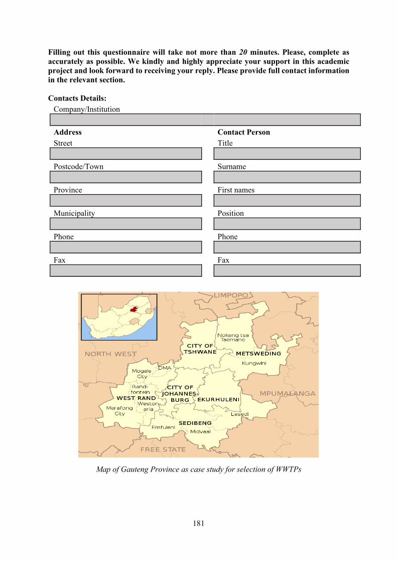
181

Filling out this questionnaire will take not more than 20 minutes. Please, complete as accurately as possible. We kindly and highly appreciate your support in this academic project and look forward to receiving your reply. Please provide full contact information in the relevant section. Contacts Details:

Company/Institution Address Contact Person Street Title Postcode/Town Surname Province First names Municipality Position Phone Phone Fax Fax

Map of Gauteng Province as case study for selection of WWTPs

182

Plant Design

1. What is the latest green drop score for the WWTP?

2. What is the latest WWTP cumulative risk rating (CRR)?

3. What is the average design capacity of WWTP in ML/day in the past 12 months?

4. What is the daily inflow of the WWTP in ML/day the last 12 months?

5. Is your plant designed to Nitrify or De-nitrify?

(indicate appropriate answer with 'X')

a) Nitrify

b) De-nitrify

6. What is the type of treated wastewater? (indicate appropriate answer with 'X')

Domestic

Industrial

Combined

7. Do you ever receive wastewater from the

following sources? (indicate appropriate answer with 'X')

i. Abattoir

ii. Food processing

plants

iii. Landfill iv. Septic tanks v. Mining plants

vi. Sources high in

fats and oil

vii. Sources of soaps

and surfactants

viii. Health care ix. Cosmetics Plants

8. How much sludge is hauled off-site on a daily basis (m3)

9. Please specify if there are anoxic or anaerobic stages and the stage/zone

Anoxic

Stage/zone

(Before, after or within the aeration tank)? Anaerobic

Stage/zone

183

10. Do organic and hydraulic loads exceed theoretical plant design capacities?

Yes

No

11. What is the typical MLSS that the sludge digester is run at? mg/l

12. What is the typical sludge age that the sludge digester is run at? days

13. Are chemicals dosed for phosphate removal? Yes No 14. Are chemicals dosed for Nitrates removal? Yes No 15. Are anti-forming agents used? Yes No

16. Are chemicals dosed directly into the aeration basins? Yes No (Please state what and approximately how much)

17. Does the plant have chemical enhanced primary

treatment (CEPT)? Yes

No

18. What is the average dissolved oxygen (DO) within the aeration basin?

19. Does the level of dissolved oxygen in the basin ever get

as low as 1.0 mgO2/l? Yes

No

20. What is the average pH of the settled sewage?

21. Does the plant have different inflows? (If the answer is Yes, kindly specify the number of inflows)

184

21. What type/s is the secondary treatment unit for nutrients removal in the WWTP?

[ Indicate appropriate answer with X in the first column and the corresponding hydraulic retention time (HRT)]:

HRT (hours)

Biological nutrients removal (BNR)

Aeration tanks Settling ponds Trickling filters Rotating biological contactors (RBC)

Membrane bioreactor (MBR)

Sequencing batch reactor (SBR)

22. Which process/es is used to treat the sludge in your WWTP? [Indicate appropriate answer with X in the first column and the corresponding hydraulic retention time (HRT):

HRT (hours) Anaerobic digestion Biogas production Gasification Pyrolysis Sludge thickening Sludge combustion Sludge draining Sludge drying Sludge processing

23. Are you aware of the waste (sludge) to energy technology (WtE)-renewable energy as a source of green (clean) energy?

Yes No

185

24. Does the plant use renewable energy technologies? Yes No

25. How do you rate the COD removal as recommended by Department of Water and Sanitation

(Water/Waste Act 49)? [Indicate appropriate answer with X] i. Poor

ii. Excellent

26. What is the major source of COD in the WWTP?

27. How do you rate the inorganic (Heavy metals) compounds removal as recommended by DWS

(Water/Waste Act 49)? [Indicate appropriate answer with X] i. Poor

ii. Excellent

28. What is the major source of trace elements in the WWTP?

29. Choose the measuring instruments used in your laboratory and on-site in the WWTP. You can

tick more than one instrument/technique if applicable [Indicate appropriate answer with X on either Laboratory or on-site]

Laboratory On-site Automatic analysers Microbial load test Chlorine measuring test COD measuring device BOD measuring device Densitometers ICP for inorganic (heavy metals) analyser Flow meters, current meters, level meters Gas analysers Gas indicators, gas detectors Gas chromatograph mass spectrometry (GC-MS) Liquid chromatograph mass spectrometry (LC-MS) High-performance liquid chromatograph (HPLC) Atomic absorption spectrometry (AAS)

186

Ion chromatography Carbon measuring instrument Calorimeter Conductimeters Flow meter Ozonometers Organic and inorganic tracer pH-value measuring devices Photometers Refractometers Oxygen content measuring devices Sludge measuring devices (Characterization of sludge: VFA, VOC, etc.) Spectrometers Thermometer Automatic titration Turbidimeters Other measuring instruments

30. The questions are about the environmental impacts of WWT technologies/processes in

your plant [Indicate appropriate answer with X].

i) Does the plant have geological impact on groundwater pollution? Yes No

ii) Does the plant experience strong odour generation? Yes No iii) Does the plant experience large amount of water

evaporation? Yes No

iv) Does the plant conduct a health safety environment (HSE) audit? Yes No

31. What are the requirements of the personal in the WWTP?

32. Specify occupational health risk in the WWTP

187

33. The following questions are about the technological/technical aspect of WWT technologies/processes in your plant. [Please indicate appropriate answer with X]

i) Is the plant performing efficiently and meeting regulatory

standards in terms of percentage removals of parameters such as COD, BOD, Total Suspended Solid (TSS), Total Phosphorus (TP), Total Nitrogen (TN), Faecal Coliforms and Heavy Metals? Yes No

ii) Does the plant have an efficient routine sampling program? Yes No iii) Does the plant have specialized and skilful personnel to handle the

WWT technologies? Yes No iv) Does the plant have a training program for staff capacity building? Yes No v) Does the plant have the capacity to handle the average organic

loading rates? Yes No vi) Does the plant accommodate excess inflow from storm water

e.g. flooding? Yes No

34. The following questions are about the economic aspect of WWT technologies/processes in your plant?

i) Does the plant have the ability to accommodate additional

operational facilities and future expansions? Yes No ii) Does the plant have sufficient funds for operation and

maintenance costs? Yes No

iii) Does the plant have sludge disposal facilities? Yes No

35. Describe any approach that you think would improve the efficiency of the plant and lower the cost of the wastewater treatment.

36. Identify any policy hindrance in the development plan, plant efficiency and regulatory standards.

Please email the electronic copies to [email protected] , [email protected] or Send hard copies to:

Dr Anthony Njuguna Matheri, Department of Chemical Engineering, University of Johannesburg, Doornfontein, Johannesburg 2028, South Africa. Office Number 4150 Cell: +27616986335 Email: [email protected] or [email protected]





188

If you would like to be kept informed of the progress of the project, then please ensure that you provide a contact name and email address at the beginning of the questionnaire.

Place, Date Signature

189

Appendix B1: The Activated Sludge Model (ASM) No. 1 under International Association of Water Quality (IAWQ)

Table B1: Process Kinetics and Stoichiometry for Carbon Oxidation, Nitrification, and Denitrification

Components i 1 2 3 4 5 6 7 8 9 10 11 12 13 Process Ratej Process S1 SS X1 XS XB,HXB,A XP SO SNO SNH SND XND SALK

1 Aerobic growth of heterotrophs 1

2 Anoxic growth of heterotrophs 1

3 Aerobic growth of autotrophs 1

4 Decay of heterotrophs -1

5 Decay of autotrophs

6 Ammonification of soluble organic nitrogen 1 -1

7 Hydrolysis of entrapped organics 1 -1

8 Hydrolysis of entrapped nitrogen 1 -1

Kinetics Parameters:

Heterotrophic growth and decay: µH, KS, KO ,H, KNO, bH

Autotrophic growth and decay: µA, KNH, KO ,A, bA

Correction factor for anoxic gowth of heterotrophs: ŋg

Ammonication: ka

Hydrolysis: kh, Kx

Correction factor for anoxic hydrolysis: ŋh

Observed Conversion Rate [ML-3T-1]

Mass N/Maas COD in product from biomass: iXP

Soluble inert organic matter [M

(CO

D)L -3)

Readily biodegrable substrate [M

(CO

D)L

-3)

Particulate inert organic matter [M

(CO

D)L -3)

Slowly biodegrable substrate [M

(CO

D)L -3)Mass N/Maas COD in biomass: iXB

Stoichiometry parameters:

Heterotrophic yield: YH

Autotrophic yield: YA

Fraction of biomass yielding particulate products: fpSoluble biodegradable organic nitrogen [M

(N)L -3)

Particulate biodegradable organic nitrogen [M(N

)L -3)

Alkalinity-M

olar units

Active heterotrophic biom

ass [M(C

OD

)L -3)

Active autotrophic biom

ass [M(C

OD

)L -3)

Particulate products arising from biom

ass decay [M(C

OD

)L -3)

Oxygen (negative C

OD

) [M(-C

OD

)L-3)

Nitrate and nitrite nitrogen [M

(N)L -3)

NH

4 ++NH

3 nitrogen [M(N

)L-3)

−1𝑌𝑌𝐴𝐴

−1𝑌𝑌𝐴𝐴

1−𝑜𝑜𝐴𝐴

1−𝑜𝑜𝐴𝐴

𝑜𝑜𝐴𝐴

𝑜𝑜𝐴𝐴

−1− 𝑌𝑌𝐴𝐴𝑌𝑌𝐴𝐴

−4.57−𝑌𝑌𝐴𝐴

𝑌𝑌𝐴𝐴

−1− 𝑌𝑌𝐴𝐴2.86𝑌𝑌𝐴𝐴

1𝑌𝑌𝐴𝐴

-𝑟𝑟𝑋𝑋𝐵

-𝑟𝑟𝑋𝑋𝐵

−𝑟𝑟𝑋𝑋𝐵−1𝑌𝑌𝐴𝐴

𝑟𝑟𝑋𝑋𝐵− 𝑜𝑜𝑃𝑟𝑟𝑋𝑋𝑃𝑟𝑟𝑋𝑋𝐵− 𝑜𝑜𝑃𝑟𝑟𝑋𝑋𝑃

𝑟𝑟𝑖𝑖 = �𝑣𝑖𝑖𝑗𝑗

𝑝𝑝𝑗

114

−𝑟𝑟𝑋𝑋𝐵14 −

17𝑌𝑌𝐴𝐴

−𝑟𝑟𝑋𝑋𝐵14

1 − 𝑌𝑌𝐴𝐴14 − 2.86𝑌𝑌𝐴𝐴

−𝑟𝑟𝑋𝑋𝐵14

𝑃𝑃7(𝑉𝑉𝑁𝐷/𝑉𝑉𝑉𝑉

𝑏𝑏𝐴𝐴𝑉𝑉𝐵,𝐴𝐴

𝑏𝑏𝐴𝐴𝑉𝑉𝐵,𝐴𝐴

𝑘𝑘𝑎𝑎𝑆𝑆𝑁𝐷𝑉𝑉𝐵,𝐴𝐴

𝑘𝑘ℎ

𝑉𝑉𝑛𝑛𝑉𝑉𝐵,𝐴𝐴

𝐾𝐾𝑋𝑋 + ( 𝑉𝑉𝑉𝑉𝑉𝑉𝐵,𝐴𝐴

)[

𝑆𝑆𝑂𝑂𝐾𝐾𝑂𝑂,𝐴𝐴 + 𝑆𝑆𝑂𝑂

)

+ (ŋℎ𝐾𝐾𝑂𝑂,𝐴𝐴

𝐾𝐾𝑂𝑂,𝐴𝐴 − 𝑆𝑆𝑂𝑂)(

𝑆𝑆𝑁𝑂𝑂𝐾𝐾𝑁𝑂𝑂 − 𝑆𝑆𝑁𝑂𝑂

)]𝑉𝑉𝐵,𝐴𝐴

μ𝐴𝐴(𝑆𝑆𝑉𝑉

𝐾𝐾𝑉𝑉 − 𝑆𝑆𝑉𝑉)(

𝑆𝑆𝑂𝑂𝐾𝐾𝑂𝑂,𝐴𝐴− 𝑆𝑆𝑂𝑂


μ𝐴𝐴(𝑆𝑆𝑁𝐴𝐴

𝐾𝐾𝑁𝐴𝐴 − 𝑆𝑆𝑁𝐴𝐴)(

𝑆𝑆𝑂𝑂𝐾𝐾𝑂𝑂,𝐴𝐴 − 𝑆𝑆𝑂𝑂


μ𝐴𝐴(𝑆𝑆𝑉𝑉

𝐾𝐾𝑉𝑉 − 𝑆𝑆𝑉𝑉)(

𝐾𝐾𝑂𝑂,𝐴𝐴𝐾𝐾𝑂𝑂,𝐴𝐴 − 𝑆𝑆𝑂𝑂

)]∗ (𝑆𝑆𝑁𝑂𝑂

𝐾𝐾𝑁𝑂𝑂 + 𝑆𝑆𝑁𝑂𝑂)ŋ𝑜𝑜𝑉𝑉𝐵,𝐴𝐴

ρ𝐽[𝑀𝑀𝐿𝐿−3𝑅𝑅−1]

190

Appendix B2: Activated Sludge Model No.1 Spreadsheet

Municipal influent

Exercise: Please fill out all cells marked with

Step 1: Available measurements in blue Step 2: calculated fractions (for data quality check)Symbol Value Unit Symbol Value Evaluation typical

CODtot TCOD 723.0 mgCOD/LCollodial CCOD 141.0 mgCOD/LParticulate COD XCOD 245.0 mgCOD/LFiltered COD SCCOD 478.0 mgCOD/L Filtered COD fraction SCCOD/TCOD 0.66 478 0.4Floc-filtered COD SCOD 337.0 mgCOD/L Floc-filtered COD fraction SCOD/TCOD 0.47 337Effluent floc-filtered COD SI 30.0 mgCOD/LTKN TKN 39.0 mgN/LNHx-N SNHx 28.0 mgN/L Ammonia fraction NHx/TKN 0.72 0.6-0.8VSS VSS 218.8 mgVSS/L COD/VSS ratio CCOD+XCCOD/VSS 1.76 1.5-1.8TSS TSS 251.0 mgTSS/L VSS/TSS ratio VSS/TSS 0.87 0.8-0.9BOD BOD 350.0 mgO2/L COD/BOD ratio TCOD/BOD 2.07 2.0-2.5Alkalinity SALK 250.0 mgCaCO3/L

green easy to measure, yellow requires some assumptions but not so important, red is important and difficult to measure

Step 3: Resulting model state variablesSoluble Species Symbol old Symbol new Value Unit Calculation Fraction of CODtot Particulate Species Symbol old Symbol new Value Unit Calculation Fraction of CODtot

Oxygen, O2 SO SO2 0.0 gO2/m3 Inert COD XI XU,Inf 94.0 gCOD/m3 XI = 13% of TCOD 0.13 Inert COD SI SU 30.0 gCOD/m3 0.04 Substrate COD XS XB 255.9 gCOD/m3 0.4 Substrate COD SS SB 307.0 gCOD/m3 (SCOD-SI) 0.42 Het BM COD XBH XOHO 36.2 gCOD/m3 XBH = 5% of TCOD 0.05 Ammonium N SNH SNHx 28.0 gN/m3 Aut BM COD XBA XANO 0.0 gCOD/m3 XBA = 0% of TCOD 0 Nitrate N SNO SNOx 0.0 gN/m3 Part XP COD XP XU,E 0.0 gCOD/m3 0 Organic N SND SB,N 5.5 gN/m3

(TKN-SNH)/2 Org Nitrogen XND XCB,N 5.5 gN/m3(TKN-SNH)/2

Alkalinity mmol SALK SAlk 5.0 mol/m3divide value in mgCaCO3/L by 50 Inorg. Suspended Solids ISS X_ISS 32.3 g ISS/m3

TSS-VSS

Step 4: Comparing model predicted combined variables with measurementsSymbol Model Measured Comment

Biodegradable COD bCOD 599.0Carbonaceous BOD5 BOD 399.3 350.0VSS VSS 218.8 218.8TSS TSS 251.0 251.0COD COD 723.0 723.0

VSS divided by measured VSS/TSS ratio. All COD states.

EvaluationAll biodegradable CODApprox. 2/3rd of bCODAll particulate COD divided by COD/VSS ratio.

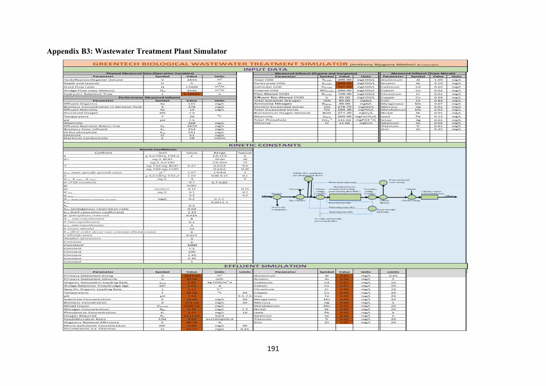
191

Appendix B3: Wastewater Treatment Plant Simulator

Parameter Symbol Value Units Parameter Symbol Value Units Parameter Symbol Value Units

Tank/Reactor/Digester Volume V 2833 m3 Total COD TCOD 495.00 mgCOD/L Aluminium Al 1.69 mg/L

Depth and Layouts H 5 m Particulate COD XCOD 245.00 mgCOD/L Arsenic As 0.10 mg/L

Fluid Flow rates Q 17000 m3/h Colloidal COD CCOD 141.00 mgCOD/L Cadmium Cd 0.02 mg/L

Sludge Flow rates (Return) Qw 4545 m3/h Filtered COD SCCOD 250.00 mgCOD/L Cobalt Co 0.02 mg/L

hydraulic Retention Time t 0.16665 h Floc-filtered COD SCOD 109.00 mgCOD/L Chromium Cr 0.01 mg/L

Effluent floc-filtered COD SI 25.00 mgCOD/L Copper Cu 0.09 mg/LParameter Symbol Value Units Total Kjeldahkl Nitrogen TKN 40.00 mgN/L Iron Fe 0.84 mg/L

Effluent Organics So 141 mg/L Ammonia Nitrogen SNHx 30.00 mgN/L Manganese Mn 0.07 mg/LBiomass Concentration in Aeration Tank X 278 mg/L Volatile Suspended Solids VSS 218.75 mgVSS/L Mercury Hg 0.01 mg/LEffluent Nutrients Xe 19 mg/L Total Suspended Solids TSS 254.36 mgTSS/L Molybdenum Mo 0.03 mg/LDissolved Oxygen DO 7.5 Biochemical Oxygen Demand BOD 271.35 mgO2/L Nickel Ni 0.01 mg/L

Temperature T 20 0C Alkalinity SALK 220.00 mgCaCO3/L Lead Pb 0.12 mg/L

pH pH 7.5 Total Phosphate PO4-3 241.00 mgPO4-3/L Silver Ag 0.01 mg/L

Alkalinity 268 mg/L Chlorine Cl 51.00 mgCl/L Selenium Se 0.05 mg/LEffluent Nutrients Return l ine XR 2670 mg/L Titanium Ti 0.01 mg/LBiomass Conc Influent Xo 254 mg/L Zinc Zn 0.25 mg/LOrtho phosphate Xve 241 mg/LChlorine Cl 51 mg/LElectrical Conductivity E 58 mS/m

Coeffient Unit Value Range Typicalk g bsCOD/g VSS.d 4 4.0-12.0 6Ks mg/L BOD 20-60 30

mg/L bsCOD 5.0-30.0 15Y mg VSS/mg BOD 0.45 0.4-0.8 0.6

mg VSS/mg COD 0.4-0.6 0.45µ m (max specific growth rate) d -1 1.07 1.0-8.0 3b g bsCOD/g VSS.d 1.04 0.06-0.15 0.1K S , K NH4 , K NO2 mg/L 9 9fv (VSS residual) 0.7 0.7-0.85fp 0.001fd unitless 0.15 0.15K O2 mg/L 0.2 0.2K max 9.5 9.5K o (half saturation constant, oxygen) mg/L 0.2 0.3-2k d 0.0011-1kn 0.3bAT (endogenous respiration rate) 0.04knT (half saturation coefficient) 1.23fp (phosphous removal) 0.025K s (micropollutant) 8b (micropollutant) 0.1µ m (micropollutant) 3k (trace metals) 12k d (first order decay rate constant-Disinfectant) 6t (disinfectant) 0.027Number of reactors 3Constant 2Constant 1000Constant 7.2Constant 100Constant 1.42Constant 2.35Constant 1

Parameter Symbol Value Units Limits Parameter Symbol Value Units Limits

Primary Settlement Sizing V 2833.00 m3 Aluminium Al 0.61 mg/L 0.05Primary Settlement Velocity V 30.00 m/h Arsenic As 0.04 mg/L 5

Organic Volumetric Loading Rate Lorg 0.85 kg COD/m3.d Cadmium Cd 0.01 mg/L 10Sludge Retention Time/Sludge Age SRT 5.04 d Cobalt Co 0.01 mg/L 20

Specific Organic Loading Rate L 1.11 h-1 Chromium Cr 0.00 mg/L 10

Temperature T 20.00 oC 44 Copper Cu 0.03 mg/L 20pH pH 7.50 5.5-7.5 Iron Fe 0.30 mg/L 20Substrate Concentration S 16.66 mg/L 30 Manganese Mn 0.03 mg/L 20Biomass Concetration X 271.13 mg/L 30 Mercury Hg 0.00 mg/L 5Mixed Liquor PXT,VSS 1500.16 mg/L Molybdenum Mo 0.01 mg/L 20Nitrogen Concentration Nae 0.35 mg/L 1.5 Nickel Ni 0.00 mg/L 20Phosphorus Concentration Pr 4.22 mg/L 10 Lead Pb 0.04 mg/L 5Oxygen Required Ro 2111.57 kd/d Selenium Se 0.00 mg/L 5Food/Microbial Ratio F/M 0.00 bsCOD/gVSS.d Titanium Ti 0.02 mg/L 20Organics Removal Efficiency E 88.18 % Zinc Zn 0.00 mg/L 20Micro-pollutants Concentration MP 0.88 mg/L 30Disinfectants (i.e. Chlorine) Cl 43.37 mg/L 0.25

GREENTECH BIOLOGICAL WASTEWATER TREATMENT SIMULATOR (Anthony Njuguna Matheri @ Copyright)

INPUT DATA

KINETIC CONSTANTS

EFFLUENT SIMULATION

Physical Measured Data (Operation Variables) Measured Influent (Organic and Inorganics)

Performance Measured Influent

Measured Influent (Trace Metals)

Kinetic Coefficients

Off-line flow equalization(for damped peak flows)

Waste backwashWaste backwash water water storage

Primary (Aeration tank/settling Secondarysettling pond/Tricking filters/RBC) settling Chlorine contact

Bar rack (Clarifier) (Clarifier) basin (Disinfection)Influent Effluent

Bar Chamber Fffluent Chlorine mixingRecycled biosolids filtration

Screen and Thickening return flowcomminution Waste biosolids

Thickening biosolids thickening

To solids and biosolids processing facilities

Grit removalBiological process

Chlorine

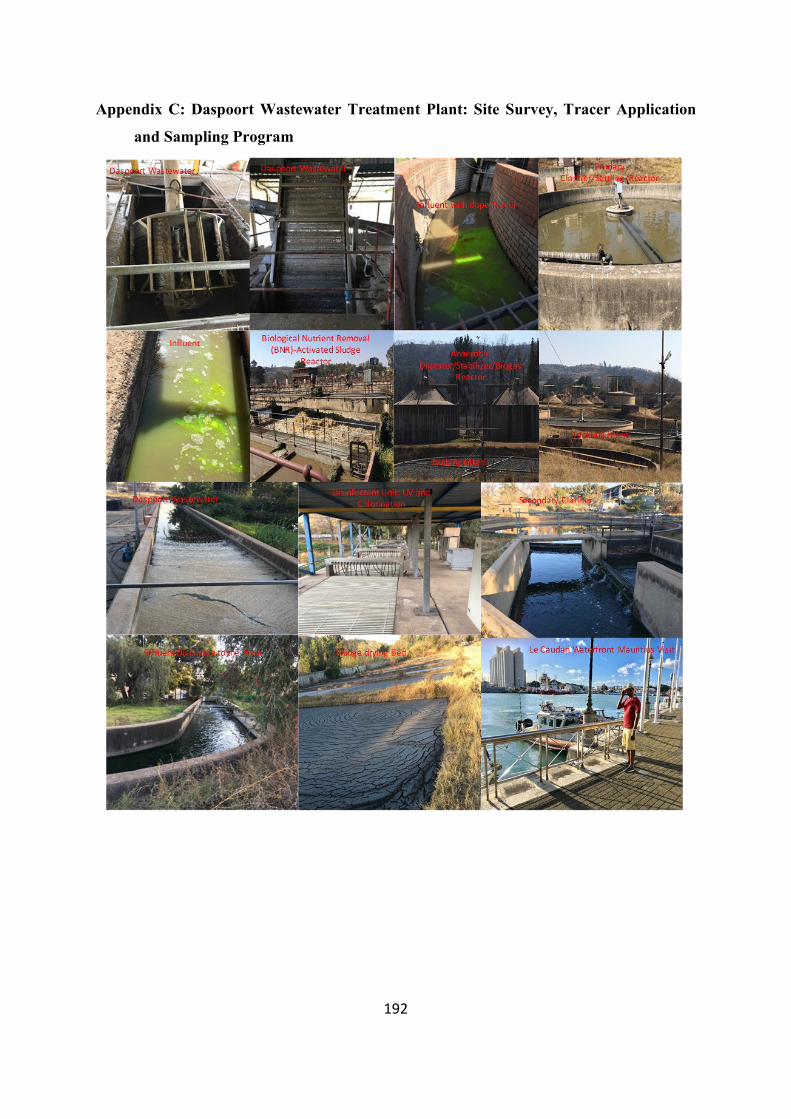
192

Appendix C: Daspoort Wastewater Treatment Plant: Site Survey, Tracer Application

and Sampling Program

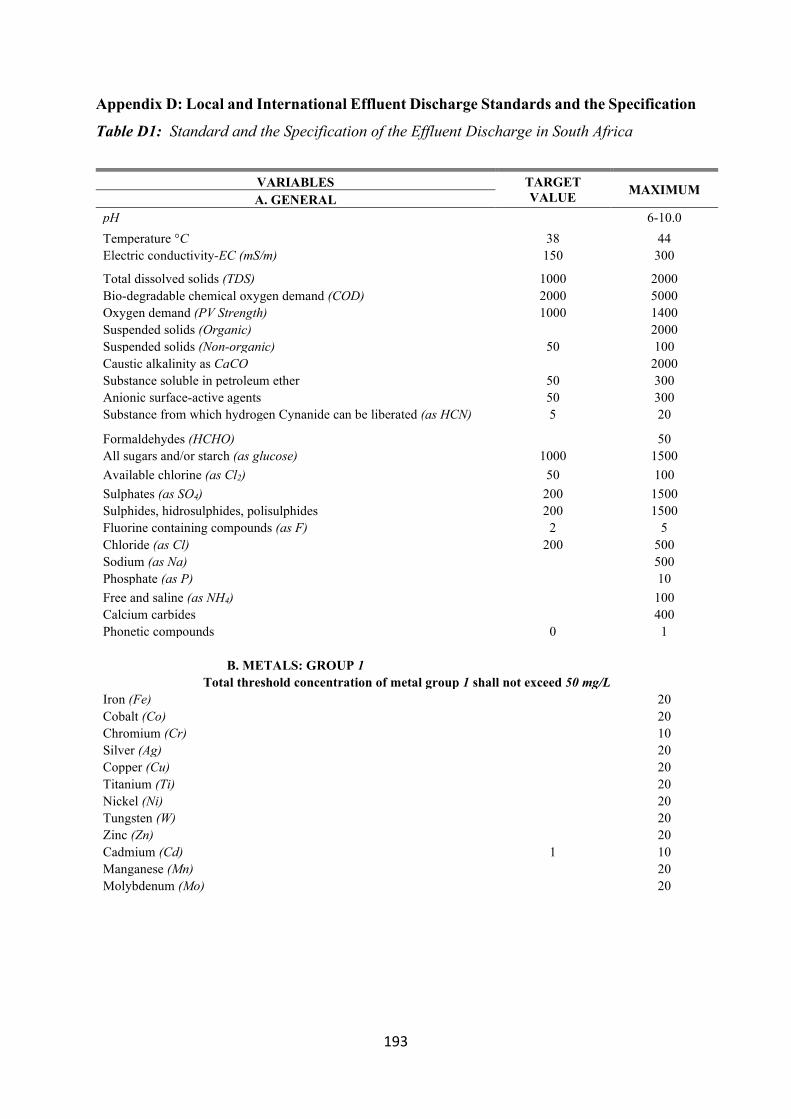
193

Appendix D: Local and International Effluent Discharge Standards and the Specification

Table D1: Standard and the Specification of the Effluent Discharge in South Africa

VARIABLES TARGET

VALUE MAXIMUM A. GENERAL

pH 6-10.0 Temperature °C 38 44 Electric conductivity-EC (mS/m) 150 300

Total dissolved solids (TDS) 1000 2000 Bio-degradable chemical oxygen demand (COD) 2000 5000 Oxygen demand (PV Strength) 1000 1400 Suspended solids (Organic) 2000 Suspended solids (Non-organic) 50 100 Caustic alkalinity as CaCO 2000 Substance soluble in petroleum ether 50 300 Anionic surface-active agents 50 300 Substance from which hydrogen Cynanide can be liberated (as HCN) 5 20

Formaldehydes (HCHO) 50 All sugars and/or starch (as glucose) 1000 1500 Available chlorine (as Cl2) 50 100 Sulphates (as SO4) 200 1500 Sulphides, hidrosulphides, polisulphides 200 1500 Fluorine containing compounds (as F) 2 5 Chloride (as Cl) 200 500 Sodium (as Na) 500 Phosphate (as P) 10 Free and saline (as NH4) 100 Calcium carbides 400 Phonetic compounds 0 1

B. METALS: GROUP 1

Total threshold concentration of metal group 1 shall not exceed 50 mg/L Iron (Fe) 20 Cobalt (Co) 20 Chromium (Cr) 10 Silver (Ag) 20 Copper (Cu) 20 Titanium (Ti) 20 Nickel (Ni) 20 Tungsten (W) 20 Zinc (Zn) 20 Cadmium (Cd) 1 10 Manganese (Mn) 20 Molybdenum (Mo) 20

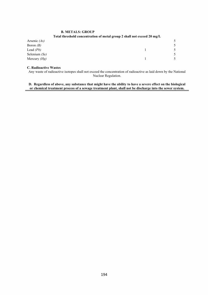
194

B. METALS: GROUP

Total threshold concentration of metal group 2 shall not exceed 20 mg/L Arsenic (As) 5 Boron (B) 5 Lead (Pb) 1 5 Selenium (Se) 5 Mercury (Hg) 1 5 C. Radioactive Wastes Any waste of radioactive isotopes shall not exceed the concentration of radioactive as laid down by the National

Nuclear Regulation.

D. Regardless of above, any substance that might have the ability to have a severe effect on the biological or chemical treatment process of a sewage treatment plant, shall not be discharge into the sewer system.

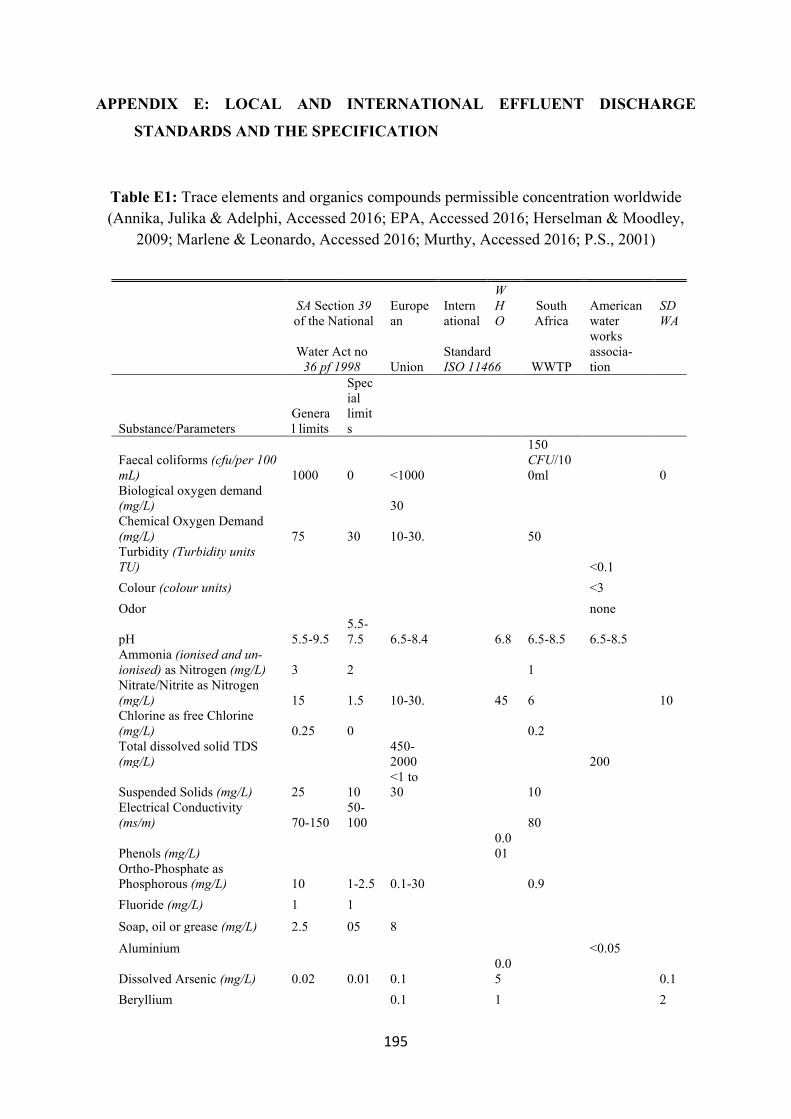
195

APPENDIX E: LOCAL AND INTERNATIONAL EFFLUENT DISCHARGE

STANDARDS AND THE SPECIFICATION

Table E1: Trace elements and organics compounds permissible concentration worldwide (Annika, Julika & Adelphi, Accessed 2016; EPA, Accessed 2016; Herselman & Moodley,

2009; Marlene & Leonardo, Accessed 2016; Murthy, Accessed 2016; P.S., 2001)

SA Section 39 of the National

European

International

WHO

South Africa

American water

SDWA

Water Act no

36 pf 1998 Union Standard ISO 11466 WWTP

works associa-tion

Substance/Parameters General limits

Special limits

Faecal coliforms (cfu/per 100 mL) 1000 0 <1000

150 CFU/100ml 0

Biological oxygen demand (mg/L) 30

Chemical Oxygen Demand (mg/L) 75 30 10-30. 50

Turbidity (Turbidity units TU) <0.1

Colour (colour units) <3 Odor none

pH 5.5-9.5 5.5-7.5 6.5-8.4 6.8 6.5-8.5 6.5-8.5

Ammonia (ionised and un-ionised) as Nitrogen (mg/L) 3 2 1

Nitrate/Nitrite as Nitrogen (mg/L) 15 1.5 10-30. 45 6 10

Chlorine as free Chlorine (mg/L) 0.25 0 0.2

Total dissolved solid TDS (mg/L)

450-2000 200

Suspended Solids (mg/L) 25 10 <1 to 30 10

Electrical Conductivity (ms/m) 70-150

50-100 80

Phenols (mg/L) 0.001

Ortho-Phosphate as Phosphorous (mg/L) 10 1-2.5 0.1-30 0.9

Fluoride (mg/L) 1 1 Soap, oil or grease (mg/L) 2.5 05 8 Aluminium <0.05

Dissolved Arsenic (mg/L) 0.02 0.01 0.1 0.05 0.1

Beryllium 0.1 1 2

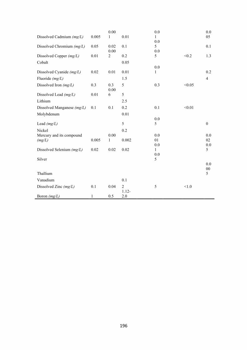
196

Dissolved Cadmium (mg/L) 0.005 0.001 0.01

0.01

0.005

Dissolved Chromium (mg/L) 0.05 0.02 0.1 0.05 0.1

Dissolved Copper (mg/L) 0.01 0.002 0.2

0.05 <0.2 1.3

Cobalt 0.05

Dissolved Cyanide (mg/L) 0.02 0.01 0.01 0.01 0.2

Fluoride (mg/L) 1.5 4 Dissolved Iron (mg/L) 0.3 0.3 5 0.3 <0.05

Dissolved Lead (mg/L) 0.01 0.006 5

Lithium 2.5 Dissolved Manganese (mg/L) 0.1 0.1 0.2 0.1 <0.01 Molybdenum 0.01

Lead (mg/L) 5 0.05 0

Nickel 0.2

Mercury and its compound (mg/L) 0.005

0.001 0.002

0.001

0.002

Dissolved Selenium (mg/L) 0.02 0.02 0.02 0.01

0.05

Silver 0.05

Thallium

0.0005

Vanadium 0.1 Dissolved Zinc (mg/L) 0.1 0.04 2 5 <1.0

Boron (mg/L) 1 0.5 1.12-2.0

197

APPENDIX F: ANALYTICAL TECHNIQUES FOR MONITORING WATER

POLLUTANTS

F1: Introduction

F1.1 Analytical techniques for monitoring water pollutants

Development and validation of novel analytical techniques for preconcentration and

determination of organic contaminants was considered. To test the robustness of the analytical

system for monitoring of organics in wastewater, three compounds in the class of parabens

were studied, namely, methylparaben, ethylparaben and propylparaben. Sample preparation

methods (extraction of analyte compounds) using solid phase extraction (SPE) methods were

studied. Analyte detection techniques based on ultra-high performance liquid chromatography

hyphenated to tandem mass spectrometry (UHPLC-MS/MS) was investigated. Experimental

factors such as sample pH, sample volume and eluent volume, were optimized using a two-

level (2k) full factorial design in conjunction with response surface methodology (RSM). The

chemometric approach is advantageous in that it decreases the number of experimental runs

resulting in reduced analysis times, reagent consumption, sample volume as well as the cost of

analysis [1]. Various extraction techniques either conventional or newly developed, were

employed for the determination of parabens in wastewater. They include dispersive liquid-

liquid microextraction (DLLME) [2], solid phase microextraction (SPME) [3], dispersive ionic

liquid (IL)-DLLME [4], magnetic solid phase extraction (MSPE) [5], rotating disk sorptive

extraction (RDSE) [1], among many others. However, the most common and robust extraction

and pre-concentration method, for extraction of parabens is solid phase extraction (SPE) [6,3].

This is largely due to its versatility in retaining these compounds and the availability of a wide

array of adsorbents, chemistries and sizes of the SPE cartridges, making it a robust and selective

extraction technique [7]. Liquid chromatography-tandem mass spectrometry (LC-MS/MS) is

the most frequently used method for determination of parabens due to its sensitivity, selectivity

and very low detection levels (µg L-1 to ng L-1) [8]. In addition, no derivatization is required as

is the case with gas chromatograhy (GC) analysis [1,9]. The UHPLC technique uses sub-2-

µm particle size columns which makes it more favourable over the traditional HPLC, as it

tremendously improves resolution with increased peak capacity and shortened analysis times

[10].

198

F2. Sample collection for analytical techniques

The analytical procedures used for sample preparation for quantification of the organic

contaminants in wastewater included sample collection; solid phase extraction (SPE),

experimental design, application of carbon nanodots in SPE. The quantification techniques

included liquid chromatography and gas chromatography hyphenated to tandem mass

spectrometry. Chemometric techniques were used for the optimization of sample extraction

procedures as per Muckoya et al. [11]. The collection of samples from WWTP in Gauteng was

done from two locations in the east and west of the plant. There were 7 sampling sites from the

east plant and 6 sampling sites on the west plant. Two samples were collected per sampling

site while observing the retention times calculated by the use of the tracer [12]. Solid phase

extraction procedure: Extraction of parabens from the wastewater samples was performed

using Oasis HLB cartridges (6 mL, 200 mg). Prior to the extraction, the samples were filtered

on a Millipore filtration unit using 0.45 µm filter paper to remove any suspended matter that

may otherwise interfere with the SPE extraction due to clogging. A multivariate experimental

design was employed for optimization of SPE experimental conditions [12]. The parameters

studied were sample volume, elution volume and sample pH. Solid phase extraction of

parabens with packed carbon nanodots (CNDs). Characterization of synthesized was done with

TEM, SEM, FTIR, XRD techniques. The carbon nanodots were synthesized according to

previous literature [13] with slight modification as per Muckoya et al. [14]. The application of

the CNDs for extraction of methyl-, ethyl- and propyl paraben (MePB, EthPB, ProPB),

azinphos-methyl and parathion-methyl from the wastewater samples, was performed using pre-

packed SPE cartridges with the CNDs. Chromatographic-mass spectrometry experimental runs

were conducted using Nexera Ultra High-Performance Liquid Chromatography (UHPLC

Shimadzu, Japan). Separation of the analytes was obtained using a pinnacle DB biphenyl

column of 100 x 2.1 mm and 3 µm particle size (RESTEK, USA). The mass spectrometry

detection was acquired in multiple reaction monitoring (MRM) mode. The detailed procedures

are given in [15].

F3. Summary Results on Analytical Techniques for Water Sample Preparation and

Analyte Detection

The WWTP East side (E1-E7) is the trickling unit and West (W1-W6) is the biological nutrients

removal (BNR) unit. The various sampling points are as shown in Table F1 where sampling

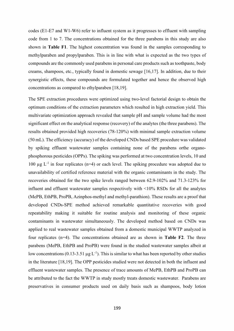
199

codes (E1-E7 and W1-W6) refer to influent system as it progresses to effluent with sampling

code from 1 to 7. The concentrations obtained for the three parabens in this study are also

shown in Table F1. The highest concentration was found in the samples corresponding to

methylparaben and propylparaben. This is in line with what is expected as the two types of

compounds are the commonly used parabens in personal care products such as toothpaste, body

creams, shampoos, etc., typically found in domestic sewage [16,17]. In addition, due to their

synergistic effects, these compounds are formulated together and hence the observed high

concentrations as compared to ethylparaben [18,19].

The SPE extraction procedures were optimized using two-level factorial design to obtain the

optimum conditions of the extraction parameters which resulted in high extraction yield. This

multivariate optimization approach revealed that sample pH and sample volume had the most

significant effect on the analytical response (recovery) of the analytes (the three parabens). The

results obtained provided high recoveries (78-120%) with minimal sample extraction volume

(50 mL). The efficiency (accuracy) of the developed CNDs based SPE procedure was validated

by spiking effluent wastewater samples containing none of the parabens orthe organo-

phosphorous pesticides (OPPs). The spiking was performed at two concentration levels, 10 and

100 µg L-1 in four replicates (n=4) or each level. The spiking procedure was adopted due to

unavailability of certified reference material with the organic contaminants in the study. The

recoveries obtained for the two spike levels ranged between 62.9-102% and 71.3-123% for

influent and effluent wastewater samples respectively with <10% RSDs for all the analytes

(MePB, EthPB, ProPB, Azinphos-methyl and methyl-parathion). These results are a proof that

developed CNDs-SPE method achieved remarkable quantitative recoveries with good

repeatability making it suitable for routine analysis and monitoring of these organic

contaminants in wastewater simultaneously. The developed method based on CNDs was

applied to real wastewater samples obtained from a domestic municipal WWTP analyzed in

four replicates (n=4). The concentrations obtained are as shown in Table F2. The three

parabens (MePB, EthPB and ProPB) were found in the studied wastewater samples albeit at

low concentrations (0.13-3.51 µg L-1). This is similar to what has been reported by other studies

in the literature [18,19]. The OPP pesticides studied were not detected in both the influent and

effluent wastewater samples. The presence of trace amounts of MePB, EthPB and ProPB can

be attributed to the fact the WWTP in study mostly treats domestic wastewater. Parabens are

preservatives in consumer products used on daily basis such as shampoos, body lotion

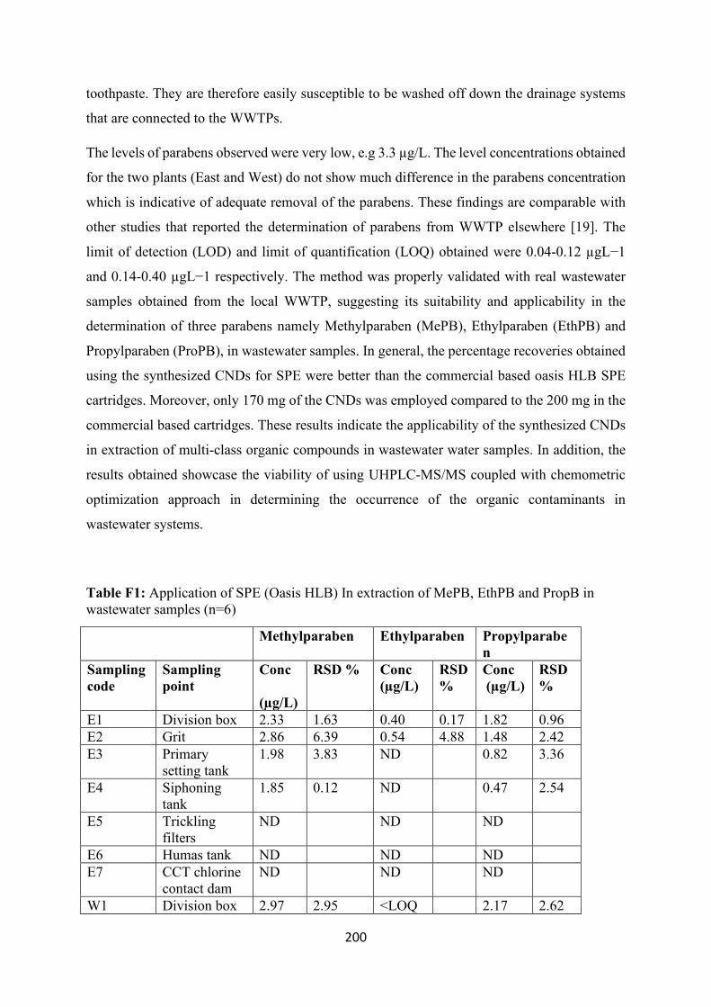
200

toothpaste. They are therefore easily susceptible to be washed off down the drainage systems

that are connected to the WWTPs.

The levels of parabens observed were very low, e.g 3.3 µg/L. The level concentrations obtained

for the two plants (East and West) do not show much difference in the parabens concentration

which is indicative of adequate removal of the parabens. These findings are comparable with

other studies that reported the determination of parabens from WWTP elsewhere [19]. The

limit of detection (LOD) and limit of quantification (LOQ) obtained were 0.04-0.12 µgL−1

and 0.14-0.40 µgL−1 respectively. The method was properly validated with real wastewater

samples obtained from the local WWTP, suggesting its suitability and applicability in the

determination of three parabens namely Methylparaben (MePB), Ethylparaben (EthPB) and

Propylparaben (ProPB), in wastewater samples. In general, the percentage recoveries obtained

using the synthesized CNDs for SPE were better than the commercial based oasis HLB SPE

cartridges. Moreover, only 170 mg of the CNDs was employed compared to the 200 mg in the

commercial based cartridges. These results indicate the applicability of the synthesized CNDs

in extraction of multi-class organic compounds in wastewater water samples. In addition, the

results obtained showcase the viability of using UHPLC-MS/MS coupled with chemometric

optimization approach in determining the occurrence of the organic contaminants in

wastewater systems.

Table F1: Application of SPE (Oasis HLB) In extraction of MePB, EthPB and PropB in wastewater samples (n=6)

Methylparaben Ethylparaben Propylparaben

Sampling code

Sampling point

Conc (µg/L)

RSD % Conc (µg/L)

RSD %

Conc (µg/L)

RSD %

E1 Division box 2.33 1.63 0.40 0.17 1.82 0.96 E2 Grit 2.86 6.39 0.54 4.88 1.48 2.42 E3 Primary

setting tank 1.98 3.83 ND 0.82 3.36

E4 Siphoning tank

1.85 0.12 ND 0.47 2.54

E5 Trickling filters

ND ND ND

E6 Humas tank ND ND ND E7 CCT chlorine

contact dam ND ND ND

W1 Division box 2.97 2.95 <LOQ 2.17 2.62

201

W2 Grit 2.30 1.86 ND 1.58 0.95 W3 Primary setter 2.56 2.25 ND 1.54 0.28 W4 BNR

activated sludge reactor

ND ND ND

W5 Humas tank ND ND ND W6 CCT chlorine

contact dam ND ND ND

ND: not detected, Conc: concentration, E: East, W: West, BNR: biological nutrients removal

Table F2: Application of proposed method on unspiked wastewater samples (n=4) Influent water Effluent water

Conc (µg/L) RSD % Conc (µg/L) Methylparaben 3.51 2.63 <LOD Ethylparaben 0.13 3.36 <LOD Propylparaben 1.46 5.44 <LOD Azinphos-Methyl <LOD <LOD Parathion-methyl <LOD <LOD

F4. Conclusions

The results obtained from optimized analytical techniques showed that, the percentage analyte

recoveries obtained using the synthesized carbon nanodots (CNDs) packing of SPE were better

than the commercial based oasis HLB SPE cartridges. Only 170 mg of the CNDs was employed

compared to the 200 mg in the commercial based cartridges. These results indicate the

applicability of the synthesized CNDs in extraction of multi-class organic compounds in

wastewater samples. For analyte quantification, UHPLC-MS/MS coupled proved to be highly

efficient when combined with chemometric optimization method in determining the presence

of the organic contaminants in wastewater systems.

F5. References

[1] Becerra-Herrera M, Miranda V, Arismendi D, Richter P (2018) Chemometric

optimization of the extraction and derivatization of parabens for their determination in water

samples by rotating-disk sorptive extraction and gas chromatography mass spectrometry.

Talanta 176:551-557

[2] Xue Y, Chen N, Luo C, Wang X, Sun C (2013) Simultaneous determination of seven

preservatives in cosmetics by dispersive liquid-liquid microextraction coupled with high

performance capillary electrophoresis. Analytical Methods 5 (9):2391-2397

202

[3] López-Darias J, Pino V, Meng Y, Anderson LJ, Afonso MA (2010) Utilization of a

benzyl functionalized polymeric ionic liquid for the sensitive determination of polycyclic

aromatic hydrocarbons; parabens and alkylphenols

in waters using solid-phase microextraction coupled to gas chromatography-flame ionization

detection. Journal of Chromatography A 1217:7189-7719. doi:10.1016/

[4] Ma T, Li Z, Jia Q, Zhou W (2016) Ultrasound‐assisted temperature‐controlled ionic liquid

emulsification microextraction coupled with capillary electrophoresis for the determination of

parabens in personal care products. Electrophoresis 37 (12):1624-1631

[5] Chen Y, Cao S, Zhang L, Xi C, Chen Z (2017) Modified QuEChERS combination with

magnetic solid-phase extraction for the determination of 16 preservatives by gas

chromatography-mass spectrometry. Food Analytical Methods 10 (3):587-595

[6] González-Mariño I, Quintana JB, Rodríguez I, Cela R (2009) Simultaneous determination

of parabens, triclosan and triclocarban in water by liquid chromatography/electrospray

ionisation tandem mass spectrometry. Rapid Communications in Mass Spectrometry 23

(12):1756-1766. doi:10.1002/rcm.4069

[7] Piao C, Chen. L, Wang Y (2014) A review of the extraction and chromatographic

determination methods for the analysis of parabens. Journal of chromatograpy B 969:139-148

[8] Pedrouzo M, Borrull F, Marcé RM, Pocurull (2009) Ultra-high-performance liquid

chromatography-tandem mass spectrometry for determining the presence of eleven personal

care products in surface and wastewaters. Journal of Chromatography A 1216 (42):6994-

7000. doi:10.1016/j.chroma.2009.08.039

[9] Zgoła-Grześkowiak A, Jeszka-Skowron M, Czarczyńska-Goślińska B, Grześkowiak T

(2016) Determination of parabens in polish river and lake water as a function of season.

Analytical Letters 49 (11):1734-1747.

[10] Jaume A, Danie lR, Bozo Z, Sandra P, Damià B (2015) Liquid Chromatography-Mass

Spectrometry quantification and confirmation aspects.

[11] Vallerie AM, Philiswa NN, Ngila* JC (2018) Factorial Design Optimisation of Solid

Phase Extraction for Preconcentration of Parabens in Wastewater Using Ultra-High

Performance Liquid Chromatography Triple Quadrupole Mass Spectrometry. Current

Analytical Chemistry 14:1-10. doi:http://dx.doi.org/10.2174/1573411014666180627150854

[12] Kunkel U, Radke M (2011) Reactive tracer test to evaluate the fate of pharmaceuticals in

rivers. Environmental science & technology 45 (15):6296-6302

[13] Leardi R (2009) Experimental design in chemistry: A tutorial. Analytica chimica acta

652 (1-2):161-172. doi:10.1016/j.aca.2009.06.015

http://dx.doi.org/10.2174/1573411014666180627150854

203

[14] Shi L, Li X, Li Y, Wen X, Li J, Choi MM, Dong C, Shuang S (2015) Naked oats-derived

dual-emission carbon nanodots for ratiometric sensing and cellular imaging. Sensors and

Actuators B: Chemical 210:533-541

[15] Albero B, Pérez RA, Sánchez-Brunete Co, Tadeo JL (2012) Occurrence and analysis of

parabens in municipal sewage sludge from wastewater treatment plants in Madrid (Spain).

Journal of hazardous materials 239-240:48-55. doi:10.1016/j.jhazmat.2012.05.017

[16] Núñez L, Tadeo JL, García-Valcárcel AI, Turiel E (2008) Determination of parabens in

environmental solid samples by ultrasonic-assisted extraction and liquid chromatography

with triple quadrupole mass spectrometry. Journal of Chromatography A 1214 (1-2):178-182.

doi:10.1016/j.chroma.2008.10.105

[17] Canosa P, Rodríguez I, Rubí E, Bollaín MH, Cela R (2006) Optimisation of a solid-

phase microextraction method for the determination of parabens in water samples at the low

ng per litre level. Journal of Chromatography A 1124 (1-2):3-10.

doi:10.1016/j.chroma.2006.03.045

[18] Regueiro J, Becerril E, Garcia-Jares C, Llompart M (2009) Trace analysis of parabens,

triclosan and related chlorophenols in water by headspace solid-phase microextraction with in

situ derivatization and gas chromatography-tandem mass spectrometry. Journal of

Chromatography A 1216 (23):4693-4702

[19] Mashile G, Mpupa A, Nomngongo P (2018) In-Syringe Micro Solid-Phase Extraction

Method for the Separation and Preconcentration of Parabens in Environmental Water

Samples. Molecules 23 (6):1450

204

APPENDIX G:

PHOTOCATALYTIC DEGRADATION OF WATER CONTAMINANTS USING

NANOMATERIALS

G1. Introduction

Photocatalysis is considered as one of the most promising technique in water treatment since it

has a great potential utilizing green and sustainable solar energy in removing organic pollutants

and harmful bacteria present in polluted water systems [31]. The photocatalytic technology

uses light and a photocatalyst (e.g metal oxide) in the decomposition of organic pollutants.

Semiconductors have been used in photocatalysis for decomposing the organic pollutants

rapidly and in an environmentally friendly manner [32-35]. Tungsten trioxide (WO3) is a

promising n-type semiconductor photocatalyst with an optical band gap (Eg) of 2.8 eV that has

received attention in recent times [36,37]. Doping of photocatalysts plays an important role in

modifying the catalyst properties. Iron (Fe) was used for doping WO3 to form Fe-doped WO3

nanocomposite material for the photodegradation of methylparaben as model organic substance

to test the efficiency of the nano-photocatalyst using advanced oxidation process [38]. WO3

was also doped with a metal chalcogenide namely, cadmium sulphide (with a small band gap

of 2.4 eV), to form CdS-WO3 for degradation of ethylparaben (EP) under solar simulated light.

The photocatalyst employed Z-scheme nanocomposite where two semiconductors are

employed as they exhibit better photoactivity due to suitable bandgap matching between the

semiconductors. Novel Z-scheme Co3O4/WO3 nanocomposite was studied for photocatalytic

degradation of ethylparaben and methylene blue under visible light irradiation. Another dopant

for WO3 investigated, was tricobalt tetroxide (Co3O4) to form Co3O4/WO3, used as a novel Z-

scheme photocatalyst Co3O4/WO3, investigated for the photodegradation of organic pollutants

namely, ethylparaben and methylene blue under simulated solar light.

G2. Nanotechnology Methods for Degradation of Organic Contaminants

Samples collected from the secondary treated water were subjected to filtration using

nanomaterials for water treatment. These nanomaterials were fabricated in our laboratory in

the Department of Applied Chemistry, University of Johannesburg. Briefly, the following

experimental procedures were employed in the preparation of nanomaterials. WO3

nanoparticles were prepared by use of microwave used by [44]. In the synthesis of Fe-doped

WO3 nanoparticles, microwave was used as per Abhudhahir and Kandasamy [44] with

modifications according to [45] producing final products for WO3 and Fe-doped WO3 as pale

205

yellow and brown, respectively. . Similar methods by [46] were used for syntheses of CdS-

doped WO3 to obtain orange powder as confirmation of CdS-WO3 nanocomposite. The

preparation of Z-scheme CO3O4/WO3 a deep green-yellow powder indicated successful

formation of CdS-WO3 nanocomposite. The synthesized nanomaterials including pristine WO3

materials, Fe-doped WO3, CdS-doped WO3, Z-scheme Co3O4-doped WO3 nanocomposites

were characterized using X-ray diffraction, Brunauer-Emmett-Teller (BET)-nitrogen

adsorption-desorption isotherms, UV-Vis diffuse reflectance spectroscopy, Raman analysis,

transmission electron microscope and high-resolution transmission electron microscopy (TEM

and HRTEM), X-ray Photoelectron Spectroscopy (XPS).

G3. Summary Results on Photocatalytic Nanomaterials for Degradation of Organics

Figure G1 shows a remarkable performance of Z-scheme Co3O4/WO3 heterojunction

photonano catalyst owing to doping of WO3 by Co3O4, and also due formation of Z-scheme

between n-type WO3 and p-type Co3O4 which aided in lowering the electron-hole pair

recombination at the interface.

It was observed that the degradation of ethylparaben by Co3O4/WO3 nanocomposite

photocatalyst can be quantified by first-order equation [54] shown in Equation G1:

− ln𝐶𝐶𝑡𝑡/𝐶𝐶𝑜𝑜 = 𝑘𝑘𝑎𝑎𝐴𝐴𝐴𝐴𝑡𝑡 Eq. G1

Where Co is the concentration of pollutants before degradation, Ct is the concentration of

pollutants at irradiation time t, and 𝑘𝑘𝑎𝑎𝐴𝐴𝐴𝐴 is the apparent kinetic coefficient (min−1) of the

degradation reaction.

The k values for degradation of EP and MB over Co3O4/WO3 was 0.0353 min-1 and 0.2558

min-1, respectively. These results represented 1.756 times higher than Co3O4 (0.0201min-1)

and 1.878 times for WO3 (0.0188 min-1) in EP and 4.490 times higher than Co3O4 (0.0575

min-1) and 3.242 times higher than bare WO3 (0.0789 min-1) in degradation of MB.

206

Figure G1: Adsorption and photodegradation of ethyl paraben (EP) and methyl blue (MB)

Co3O4, WO3, and by Z-scheme Co3O4/WO3 nanocomposite

G4. Conclusions

Degradation of parabens and methyl blue in the wastewater using photocatalyst nanomaterials

was investigated using tungsten trioxide (WO3) modified with various dopants. The

photodegradation by-products were analysed with LC-MS/MS to identify and quantify these

products. The novel Z-scheme Co3O4/WO3 nanocomposite proved to be an excellent candidate

for the photocatalytic degradation of organic pollutants. Pollutant removal efficiency of 99%

was achieved when secondary treated water was subjected to in-house fabricated nanosorbents

as filters.

G5. References

[1] Che H, Liu C, Hu W, Hu H, Li J, Dou J, Shi W, Li C, Dong H (2018) NGQD active sites

as effective collectors of charge carriers for improving the photocatalytic performance of Z-

scheme g-C3N4/Bi2WO6 heterojunctions. Catalysis Science & Technology 8 (2):622-631.

doi:10.1039/C7CY01709J

[2] Ye L, Su Y, Jin X, Xie H, Zhang C (2014) Recent advances in BiOX (X= Cl, Br and I)

photocatalysts: synthesis, modification, facet effects and mechanisms. Environmental

Science: Nano 1 (2):90-112

[3] Dong S, Feng J, Fan M, Pi Y, Hu L, Han X, Liu M, Sun J, Sun J (2015) Recent

developments in heterogeneous photocatalytic water treatment using visible light-responsive

photocatalysts: a review. RSC Advances 5 (19):14610-14630. doi:10.1039/C4RA13734E

(a) (b)

207

[4] Wen Z, Wu W, Liu Z, Zhang H, Li J, Chen J (2013) Ultrahigh-efficiency photocatalysts

based on mesoporous Pt-WO3 nanohybrids. Physical Chemistry Chemical Physics 15

(18):6773-6778. doi:10.1039/C3CP50647A

[5] Che H, Che G, Dong H, Hu W, Hu H, Liu C, Li C (2018) Fabrication of Z-scheme

Bi3O4Cl/g-C3N4 2D/2D heterojunctions with enhanced interfacial charge separation and

photocatalytic degradation various organic pollutants activity. Applied Surface Science

455:705-716. doi:https://doi.org/10.1016/j.apsusc.2018.06.038

[6] Adhikari S, Sarkar D (2014) Hydrothermal synthesis and electrochromism of WO3

nanocuboids. RSC Advances 4 (39):20145-20153. doi:10.1039/C4RA00023D

[7] Qian J, Zhao Z, Shen Z, Zhang G, Peng Z, Fu X (2016) Oxide vacancies enhanced visible

active photocatalytic W19O55 NMRs via strong adsorption. RSC Advances 6 (10):8061-8069.

doi:10.1039/C5RA23655J

[8] Ahmed Y, Yaakob Z, Akhtar P (2016) Correction: Degradation and mineralization of

methylene blue using a heterogeneous photo-Fenton catalyst under visible and solar light

irradiation. Catalysis Science & Technology 6 (4):1233-1233. doi:10.1039/C6CY90011A

[9] Sayed Abhudhahir MH, Kandasamy J (2015) Synthesis and characterization of

Manganese doped Tungsten oxide by Microwave irradiation method. Materials Science in

Semiconductor Processing 40:695-700. doi:http://dx.doi.org/10.1016/j.mssp.2015.07.031

[10] Ngigi EM, Nomngongo PN, Ngila JC (2019) Synthesis and Application of Fe-Doped

WO 3 Nanoparticles for Photocatalytic Degradation of Methylparaben Using Visible-Light

Radiation and H 2 O 2. Catalysis Letters 149 (1):49-60

[11] Ngigi EM, Kiarii EM, Nomngongo PN, Ngila CJ (2018) Application of Z-Scheme CdS

WO3 Nanocomposite for Photodegradation of Ethylparaben under Irradiation with Visible

Light: A Combined Experimental and Theoretical Study. ChemistrySelect 3 (34):9845-9856

[12] Li K, Liang Y, Yang J, Zhang H, Yang G, Lei W (2018) BiOCl/Fe2O3 heterojunction

nanoplates with enhanced visible-light-driven photocatalytic performance for degrading

organic pollutants and reducing Cr(VI). Journal of Photochemistry and Photobiology A:

Chemistry 364:240-249. doi:https://doi.org/10.1016/j.jphotochem.2018.06.001

https://doi.org/10.1016/j.apsusc.2018.06.038

http://dx.doi.org/10.1016/j.mssp.2015.07.031

https://doi.org/10.1016/j.jphotochem.2018.06.001

MATHEMATICAL MODELLING FOR BIOLOGICAL ...

Documents