Mathematical model of geometry and fibrous structure of the heart

Mathematical model of geometry and fibrous structure of the heart

P. M. F. NIELSEN, I. J. LE GRICE, B. H. SMAILL, AND P. J. HUNTER Department of Engineering Science, School of Engineering, and Department of Physiology, School of Medicine, University of Auckland, Auckland, New Zealand

NIELSEN, P. M. F., I. J. LE GRICE, B. H. SMAILL, AND P. J. HUNTER. Mathematical model of geometry and fibrous structure of the heart. Am. J. Physiol. 260 (Heart Circ. Physiol. 29): H1365-H1378,1991.-We developed a mathematical representation of ventricular geometry and muscle fiber organization using three-dimensional finite elements referred to a prolate spheroid coordinate system. Within elements, fields are approximated using basis functions with associated parameters defined at the element nodes. Four parameters per node are used to describe ventricular geometry. The radial coordinate is interpolated using cubic Hermite basis functions that preserve slope continuity, while the angular coordinates are interpolated linearly. Two further nodal parameters describe the orientation of myocardial fibers. The orientation of fibers within coordinate planes bounded by epicardial and endocardial surfaces is interpolated linearly, with transmural variation given by cubic Her- mite basis functions. Left and right ventricular geometry and myocardial fiber orientations were characterized for a canine heart arrested in diastole and fixed at zero transmural pressure. The geometry was represented by a 24-element ensemble with 41 nodes. Nodal parameters fitted using least squares provided a realistic description of ventricular epicardial [root mean square (RMS) error < 0.9 mm] and endocardial (RMS error < 2.6 mm) surfaces. Measured fiber fields were also fitted (RMS error < 17”) with a 60-element, 99-node mesh obtained by subdividing the U-element mesh. These methods provide a compact and accurate anatomic description of the ventricles suitable for use in finite element stress analysis, simulation of cardiac electrical activation, and other cardiac field modeling problems.

finite element model; ventricular geometry; myocardial fiber orientation

A MATHEMATICAL MODEL of cardiac architecture, which provides realistic descriptions of both the geometry of left and right ventricles and the organization of muscle fibers within the ventricular myocardium, is necessary for quantitative analysis of many aspects of cardiac function. In particular, such a model is required for finite element analysis of cardiac stress and deformation (33) and the simulation of cardiac electrical activation (19).

The first attempts to model cardiac geometry concen- trated solely on the left ventricle and treated it as a thick-walled axisymmetric shell. It was argued that the

epicardial and endocardial surfaces of the left ventricle could be represented as truncated confocal prolate spheroids (4, 5, 27). More detailed reconstructions of dynamic left ventricular geometry were obtained from anterior or posterior cineangiographic projections of the left ventricle, again assuming axial symmetry (8).

Full three-dimensional reconstructions of left ventricular geom etry have been obtained using a variety of imaging methods. These include biplane cineangiography (3, 18, 31, 32) and two-dimensional ultrasound (7). In addition, a special purpose computer tomography system has been used to image right and left ventricles in the beating heart (21). It was not possible to identify a well- defined reference state in any of these studies, and this has limited the utility of the geometric data obtained. However, conventional anatomic techniques have been adapted to obtain more detailed information from serial sections of the right and left ventricles (12, 15, 16).

In many of the studies described above, finite element meshes have been fitted to reconstructed spatial coordinates to represent ventricular epicardial and endocardial surfaces. However, these models provide an incomplete description of cardiac architecture. In no case is there a realistic three-dimensional representation of right and left ventricular geometry that also incorporates an accurate description of myocardial fiber distributions.

The first quantitative measurements of fiber orientation through the heart wall were made by Streeter and Bassett (26). They found a smooth transmural variation of fiber orientation and argued that the myocardium was a continuum rather than an assembly of discrete fiber bundles, as had been postulated by MacCallum (13) and Mall (14). Since this time there have been numerous studies of myocardial fiber orientation in a variety of species (1, 6, 9, 23, 28, 29). In these studies, muscle fiber orientation was mapped out at a limited number of transmural ventricular sites, and fiber architecture was not quantitatively referred to ventricular geometry. The data obtained therefore provide a limited and essentially qualitative description of cardiac fiber distribution within the myocardium.

Two methods intended to provide more comprehensive information on cardiac muscle fiber organization have

0363-6135/91 $1.50 Copyright 0 1991 the American Physiological Society H1365

H1366 FINITE ELEMENT MODEL OF CARDIAC ANATOMY

been reported (15, 16). Both involve three-dimensional reconstruction of muscle architecture from fiber paths in serial sections. In the first of these studies (X5), fiber orientation was obtained at a limited number of sites only. The more recent approach of McLean et al. (16), in which fiber paths are tracked in serial transverse or longitudinal planes, has the limitation that both orthogonal planes cannot be studied in a single heart.

In summary, there is a clear need to develop improved measurement techniques to characterize cardiac architecture. Moreover, if the data obtained are to be of general use, then they must be reduced to an efficient mathematical representation. The objective of this study was to establish a compact and realistic finite element model of the geometry and the fibrous organization of the left and right ventricles in a well-defined reference state. It is intended that this model should be used for finite element stress analysis, the simulation of cardiac electrical activation, and for any other field problem requiring an accurate anatomic description of the heart.

MATHEMATICAL MODEL

We adopt the standard piecewise polynomial approximation methods characteristic of the finite element method (35). We use a prolate spheroidal coordinate system rather than rectangular Cartesian coordinates because the prolate spheroid provides a good initial approximation to ventricular boundary geometry and per- mits the use of a linear least-squares fitting algorithm in which only the radial (X) coordinate is fitted (see below).

A material point in the myocardium described by the coordinates (X, p, 8) has rectangular Cartesian coordinates

X = a cash X cos p

Y = a sinh X sin p cos 0

2 = a sinh X sin ,u sin 8

where a is the location of the focus on the x-axis, as shown in Fig. IA.

The true position of a material point, identified by material coordinates (&, &, &) within an element, is approximated by an interpolation of parameters defined at the element nodes. For linear interpolation, these parameters are simply the values of the coordinates at the nodes (X,, pu,, &). Thus a trilinear interpolation of the nodal values of the O-coordinate is

et&, 42, (3) = Ll&>Ll(42)Ll(t3)~1 + L2(tl&l(t2@&3)~2

+ Ld~d-'2(f2)Ll(~3>~3 + L2(4‘1&2(t2>Ll(t3)~4

+ Ll&>Ll($2)L2(~3)& + L2(tl)Ll(f2)L2(t3>& (1)

+ Ll&)L2(f2&2(t3>& + L2(tl)L2(t2>L2(t3h

where L&) = 1 - 4 and L,(t) = 4 are one-dimensional linear Lagrange basis functions (35). The element material coordinates &, t2, and [3 are chosen to lie in the circumferential, azimuthal, and transmural directions, respectively, as shown in Fig. 1E

The use of nodal parameters and their associated basis functions, rather than a polynomial representation 8 = a +bL+cL+.... has the twofold advantage of ensuring

interelement continuity without the need for explicit constraints and providing parameters that have an immediate physical interpretation (0, are the O-coordinate values at node n).

The prolate spheroidal p-coordinate is also interpolated with linear Lagrange basis functions. However, to achieve first-order continuity (i.e., continuity of slope) between elements we use bicubic Hermite basis functions (35) for interpolating the X-coordinate in the (41, &)- plane

+ H?&)f@4[2)~3 + H;(El)H%[2)~4

where the one-dimensional cubic Hermite basis functions are defined by

dX aA The interpolation of the first derivatives F and F

1 2

d"X and cross derivative -

@1@2

at the element nodes would

aA dX ensure continuity of - and - throughout the model if

at 1 at 2

elements were evenly spaced. However, because & is an dX

element coordinate, the value of - at one element vertex at 1

dX will not necessarily be the same as the value of - at the

at 1

vertex of an adjacent element associated with the same global node. We therefore define the derivative of X with respect to the arc length sl in the &-direction at the

dX global nodes, as,

dX and define the element derivative -

1 at 1

bY

ah aX dsl ---- - at 1 as1 &

ds where 1

& is an element scaling factor that accounts for

FINITE ELEMENT MODEL OF CARDIAC ANATOMY H1367

the difference in &-spacing with arc length in contiguous elements. (Notice that sl, by definition, does not vary with &.) A similar argument holds for &, giving

ah aX dsZ -E-P at 2 as2 a2

and

a2X d2X dsI ds2 - = --- Wf2 aSlaS2 & dt2

aX aX a% The parameters X, g, z, and ds defined at the

1 2 12

nodes of the finite element mesh, together with the ds ds

element scaling factors 1 and 2 and the interpolation a 1 dt 2

functions given above (trilinear for 8 and p, bicubic Hermite linear for X, in the &, t2, & material element coordinates), define the myocardial geometry.

To fit a finite element mesh to the measured geometry of the epicardial and endocardial surfaces of the heart, the nodal values of 0 and p were held fixed and the nodal

aX aii values of X, - -, and

a% asl' as2

- were fitted using a least- aSIdS

squares algorithm described below. To model the muscle fiber orientations, we assume

that the fibers lie in (&, t2)-coordinate planes and sub- tend an angle v with the (circumferential) &coordinate. The angle q is then given by an interpolation of nodal parameters at the same node positions used to define the geometry.

The basis functions used to interpolate q within an element were chosen to give linear interpolation in & and t2 (in the plane of the wall; Fig. 1) and cubic Hermite interpolation in 43 (transmurally). Similar to the geometric variable derivatives, the fiber angle cubic Hermite element derivative must be obtained from its global node counterpart by using an element scaling factor

a?? ar ds3 -c-P at 3 as3 a3

ar The nodal values of q and g were fitted by least squares

3

FIG. 1. Cardiac prolate spheroid coordinate system. A: prolate spheroid coordinate system (X, p, 8) in relation to rectangular coordinates (x, y, z); a is focus. Ellipsoid of revolution about x- axis is represented by X = constant. B: element material coordinates (&, &, [a) lie in circumferential, azimuthal, and radial directions, respectively.

to the fiber angle measurements after the geometric fit, using a more refined mesh than that needed for the geometric data (see below).

METHODS

Experimental preparation. Mongrel dogs weighing 20- 33 kg were anesthetized with 25 mg/kg thiopental sodium and maintained with oxygen and 2% halothane using positive-pressure ventilation. A thoracotomy was per- formed, and a ligature was placed loosely around the ascending aorta. The ligature was tightened as a 50-ml bolus of 15% potassium citrate at 4°C was injected rapidly into the left ventricle via a 14-gauge needle inserted through the apex, causing immediate cardiac arrest in diastole.

The heart was rapidly excised and suspended vertically from points around the base in cold (1OOC) 0.9% NaCl solution. The atria and pulmonary trunk were cut away, and the aorta was transected 20-30 mm above the aortic valve. Left and right coronary arteries were cannulated, and the coronary circulation was flushed with cold car- dioplegic solution (30). The heart was then immersed in 3% formaldehyde in phosphate buffer (room tempera- ture) while the coronary circulation was perfused with the formaldehyde solution for 30 min at a pressure of 13 kPa. Because the heart was held at neutral buoyancy in a fluid, ventricular transmural pressure was zero and fixation occurred in a well-defined unloaded state.

To prepare the heart for measurement, a stainless steel spindle was inserted through the fibrous tissue between the mitral and aortic valves and through the apex (the origin of the left ventricular vortex). This formed the longitudinal axis to which geometric data was initially referenced. A circular stainless steel end plate was located on the spindle. Pins were passed through the valve orifices into right and left ventricular cavities, positioned in radial slots milled in the end plate, and locked in place. Both ventricular cavities were then filled with silicone rubber (Dow Corning RTE) under gravity. The end plate assembly ensured that the heart was firmly located with respect to the spindle even when parts of the myocardium were later dissected away.


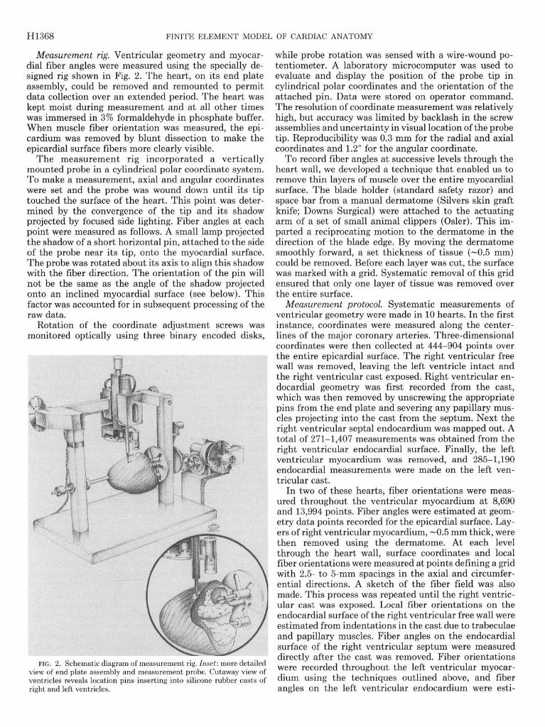
Measurement rig. Ventricular geometry and myocar- while probe rotation was sensed with a wire-wound po- dial fiber angles were measured using the specially de- tentiometer. A laboratory microcomputer was used to signed rig shown in Fig. 2. The heart, on its end plate evaluate and display the position of the probe tip in assembly, could be removed and remounted to permit cylindrical polar coordinates and the orientation of the data collection over an extended period. The heart was attached pin. Data were stored on operator command. kept moist during measurement and at all other times The resolution of coordinate measurement was relatively was immersed in 3% formaldehyde in phosphate buffer. high, but accuracy was limited by backlash in the screw When muscle fiber orientation was measured, the epi- assemblies and uncertainty in visual location of the probe cardium was removed by blunt dissection to make the tip. Reproducibility was 0.3 mm for the radial and axial epicardial surface fibers more clearly visible. coordinates and 1.2” for the angular coordinate.

The measurement rig incorporated a vertically To record fiber angles at successive levels through the mounted probe in a cylindrical polar coordinate system. heart wall, we developed a technique that enabled us to To make a measurement, axial and angular coordinates remove thin layers of muscle over the entire myocardial were set and the probe was wound down until its tip surface. The blade holder (standard safety razor) and touched the surface of the heart. This point was deter- space bar from a manual dermatome (Silvers skin graft mined by the convergence of the tip and its shadow knife; Downs Surgical) were attached to the actuating projected by focused side lighting. Fiber angles at each arm of a set of small animal clippers (Osler). This im- point were measured as follows. A small lamp projected parted a reciprocating motion to the dermatome in the the shadow of a short horizontal pin, attached to the side direction of the blade edge. By moving the dermatome of the probe near its tip, onto the myocardial surface. smoothly forward, a set thickness of tissue (-0.5 mm) The probe was rotated about its axis to align this shadow could be removed. Before each layer was cut, the surface with the fiber direction. The orientation of the pin will was marked with a grid. Systematic removal of this grid not be the same as the angle of the shadow projected ensured that only one layer of tissue was removed over onto an inclined myocardial surface (see below). This the entire surface. factor was accounted for in subsequent processing of the Measurement protocol. Systematic measurements of raw data. ventricular geometry were made in 10 hearts. In the first

Rotation of the coordinate adjustment screws was instance, coordinates were measured along the center- monitored optically using three binary encoded disks, lines of the major coronary arteries. Three-dimensional

coordinates were then collected at 444-904 points over the entire epicardial surface. The right ventricular free wall was removed, leaving the left ventricle intact and the right ventricular cast exposed. Right ventricular endocardial geometry was first recorded from the cast, which was then removed by unscrewing the appropriate pins from the end plate and severing any papillary muscles projecting into the cast from the septum. Next the right ventricular septal endocardium was mapped out. A total of 271-1,407 measurements was obtained from the right ventricular endocardial surface. Finally, the left ventricular myocardium was removed, and 2851,190 endocardial measurements were made on the left ventricular cast.

In two of these hearts, fiber orientations were measured throughout the ventricular myocardium at 8,690 and 13,994 points. Fiber angles were estimated at geometry data points recorded for the epicardial surface. Lay- ers of right ventricular myocardium, -0.5 mm thick, were then removed using the dermatome. At each level through the heart wall, surface coordinates and local fiber orientations were measured at points defining a grid with 2.5 to 5-mm spacings in the axial and circumferential directions. A sketch of the fiber field was also made. This process was repeated until the right ventricular cast was exposed. Local fiber orientations on the endocardial surface of the right ventricular free wall were estimated from indentations in the cast due to trabeculae and papillary muscles. Fiber angles on the endocardial surface of the right ventricular septum were measured

FIG. 2. Schematic diagram of measurement rig. Inset: more detailed directly after the cast was removed. Fiber orientations

view of end plate assembly and measurement probe. Cutaway view of were recorded throughout the left ventricular myocar-

ventricles reveals location pins inserting into silicone rubber casts of dium using the techniques outlined above, and fiber right and left ventricles. angles on the left ventricular endocardium were esti-


mated from the left ventricular cast. Data fitting. The choice of a polar coordinate system

for describing the geometry of the heart has a major benefit when fitting the nodal coordinates of the model to the surface measurements, because only the radial coordinate need enter the least-squares fitting procedure. However, even with a polar coordinate system, the surface coordinates ([f, 6:) obtained from the orthogonal projection of data point d onto the model surface change as the finite element ensemble is moved from the initial configuration to one minimizing the sum of squared projection lengths. For fitting the heart surface measurements, this change can be minimized by adopting a prolate spheroidal coordinate system (Fig. 3). If it is assumed that the coordinates ([f, [f) for each data point do not change at all from their initial values, then a linear-fitting procedure may be obtained by minimizing the sum of squares (S)

s = c w,[x([;“, [if) - b12 (3)

where Ad is the X-coordinate of the measured point d, A([?, [$) is the X-coordinate of the projection-of data point d onto the model surface along lines of constant p and 8, and wd is a weight associated with data point d. A@, t$) is given by a bicubic Hermite interpolation of

a~, aX, d”X, the nodal parameters X,, -, -, and -

as1 as2 ds ds . Although

12

minimizing the sum of squares given by Eq. 3 is not the same as minimizing a Euclidean norm, the difference in fitting surface parameters is negligible in comparison with mean measurement error, and the computational cost of this linear fitting procedure is orders of magnitude less than the cost of the nonlinear procedure (17).

The arc lengths s1 and s2 are defined to be linear with respect to & and 42, respectively, in the initial unfitted finite element mesh and not altered during the fitting procedure. Because 8 and p are constrained to be linear in & and t2 by the choice of basis function, & and 42 are linear in 8 and p and therefore cannot be linear in arc length on the fitted mesh. Thus s1 and s2 should be interpreted not as physical arc lengths but as arbitrary parameters specified along the & and t2-coordinate directions, respectively, which provide the connection between global derivatives and element derivatives in the

Initial finite element ensemble .

>- Final ensemble .w

ata point onto h coordi nate

FIG. 3. Schematic diagram of linear least-squares fit of finite element ensemble to geometric data in prolate spheroid coord .inate system.

cubic Hermite interpolation. They are arbitrary to the 81 dsl

extent that they only appear in products such as - - as1 dE1

and can therefore be scaled by an arbitrary multiplicative constant, provided the scaling is applied consistently. If &-coordinate lines were to follow p = constant trajectories and t2-coordinate lines were to follow 0 = con .stant trajectories, then we c ould choose s1 to be 8 and s2 to be p. However, this is not possible here where, for example, the boundaries of the right ventricle are modeled by t2- coordinate lines that vary with both 8 and p.

An ensemble of 24 bicubic elements was used to fit the geometry of left and right ventricles (Fig. 4). The free wall of the right ventricle was represented by 4 elements, the interventricular septum was represented by 4 elements, and the remaining 16 elements were used to describe the balance of the left ventricular myocardiu .m. With this ensemble topology, 52 degrees of freedom were available as fitting parameters for the epicardial surface, while left and right endocardial surfaces were fitted using 52 and 44 parameters, respectively. Bicubic Hermite elements ensured that first-order continuity of the radial coordinate was maintained over all surfaces.

The nodes defining the right ventricular boundaries (where free and septal endocardial surfaces become continuous) require special attention, as there are surface data only to one side of these nodes. The surface derivatives at these sites were very sensitive to local surface irregularities. We therefore allowed X at these nodes to enter the fit to the local surface data but fixed the derivative at the adjacent epicardial value. This con- straint is not unreasonable, as the thin-walled right ventricle at its borders is parallel to the epicardium.

-Y

FIG. 4. Schematic diagram of finite element mesh. Node numbers are shown. Free wall of right ventricle is represented by 4 elements (nodes 1, 2, 4, 5, 6, 8, 9, 10, 12, 14, 15, 17, 19, 20, 22, 24, 25, 27).


It was necessary to preprocess the raw data before fitting. The local surface orientation was determined at each measurement point, which enabled us to estimate the true fiber orientation from the recorded angle (see APPENDIX). The geometric data was then transformed from the original cylindrical polar coordinates to prolate spheroidal coordinates. The closest approximation of the aortic and mitral valves was set to an azimuthal coordinate of 120”. The focal position for the prolate spheroidal coordinate system was set so that the radial coordinate of the apex assumed a value of unity. In practice this provided a convenient method for normalizing the heart, allowing direct comparison of the geometry of different- sized hearts. The zero point of the rotational coordinate was set to the average of the right ventricular measurements. The above transformation to prolate spheroidal coordinates ensured that the hearts were described in a well-defined reference configuration, eliminating the differences that might occur in mounting hearts on the measurement rig.

Because the measured fiber angles showed rapid changes in the circumferential direction at the boundaries of the right ventricle, we chose to use a 60-element, 99-node mesh obtained by subdividing the 24-element mesh used to fit the geometry. With this more refined mesh, having 10 elements circumferentially, 3 axially, and 2 transmurally, it was found that linear interpolation in the (&, &)-coordinates and cubic Hermite interpolation in the &-coordinate provided sufficient degrees of freedom to represent the fiber field data with acceptable accuracy.

The three-dimensional fiber field parameters were found by first fitting the epicardial, left ventricular endocardial, and right ventricular endocardial surfaces with bilinear surface variation of the surface node q-parameters and then fitting the transmural myocardial fiber measurements with the remaining interior node values of q together with the complete set of nodal derivatives

d17

dss l

The surface fits were obtained by projecting the surface fiber angle measurements onto the adjacent fitted geometric surface. This strategy was required to obtain accurate epicardial and endocardial fits in regions where the fiber angle changed rapidly near the surface and the model geometry did not exactly match the real heart. For example, if fiber data at some point on the real epicardium lay slightly outside the model epicardium they would not be included in a three-dimensional fit, with the result that the model fiber distribution at that point on the model surface would reflect subendocardial fiber angles rather than the (possibly quite different) epicardial fiber angles. An alternative strategy for coping with this problem is to extend the basis function defini- tions outside the element boundaries so that data exter- nal to the model would be included in the fit [see Nielsen

W)l. Fiber angle data are only unique within a principal

angle range of 180”. It is sometimes necessary to adjust the principal angle of the data to ensure that the restricted principal value range does not produce artifac-

tual discontinuities of angle for data in which the fiber angle is in fact varying smoothly around the ventricles and through the wall. Use of the conventional principal angle range for fiber orientation creates problems at the junction of the right ventricular free wall and the ventricular septum. In the right ventricular free wall, fiber orientation typically varies from -60” at the epicardium to +90” at the endocardium, whereas in the septal wall the fiber angle ranges from about -90” at the right ventricular endocardium to around +80” at the left ventricular endocardium. On either side of the right ventricular border, therefore, the principal angle for endocardial fibers with a common orientation differs by 180”. To accommodate this abrupt change in principal value, three nodes are used at each of these right ventricular border sites: one for the right ventricular free wall, one for the septal wall, and one for the adjacent left ventricular free wall. The latter is used because there is, in fact, a real discontinuity in fiber angle due to the merging of right ventricular free wall and septal fibers with left ventricular fibers. This required 2 extra nodes at 9 sites giving a total of 117 nodes used in the fiber fits. We also localized the errors due to these discontinuities by decreasing the size of the elements at these sites.

RESULTS

Ventricular geometry. The ensemble of 24 bicubic elements provides an excellent representation of the geometry of right and left ventricles. In Fig. 5A, measurements of epicardial surface geometry are projected onto the initial prolate spheroid mesh. The same data points in Fig. 5B are projected onto the best-fit epicardial surface mesh. Projection vectors in Fig. 5B cannot be observed due to the goodness of fit.

The accuracy with which the smooth epicardial surface was fitted is indicated by the root mean square error, which was CO.9 mm in all cases. The finite element ensembles fitted to the endocardial surfaces of left and right ventricles provide a realistic description of major structures, such as the papillary muscles, but smooth out the sharp dimensional variations characteristic of the endocardium. Thus there were significant variations in local fitting error because of the presence of deep trabe- culations that could not be represented. The root mean square errors for right and left ventricular endocardial surface fits were ~2.1 and 2.6 mm, respectively.

The resolution of these surface meshes in the &- and &-directions (4 elements circumferentially and 3 elements axially) was chosen in conjunction with the basis functions such that the mean fitting error was comparable with the mean measurement error for the surface data. Figure 6 shows a plot of fitting error vs. degrees of freedom for the epicardium with 2, 4, 8, and 16 elements in the & (circumferential)-direction and 3, 6, and 12 elements in the & (axial)-direction, both for bilinear and bicubic basis functions. The results are given in Table 1. Notice that the 12-element bicubic mesh lies close to the knee of the curve. Doubling the number of degrees of freedom reduces the error by lo%, whereas halving the number of degrees of freedom increases the error by 400%.


FIG. 5. Least-square fitting of finite element nodal X-parameters to epicardial geometry measurements. Data points projected onto initial prolate spheroid (A) and optimized finite element surface mesh (23). Dotted line projections are from data points to sites on mesh with same p, O-coordinates.

5-

. n Bilinear basis

Lg. + Bicubic basis

z + 4 x 3 Elements

-3-.m . bicubic basis

; - ++ k

+

Q) 2-

H

n

: w

l- + 9 4

$

0 . I . I I 1 . 1

0 100 200 300 400

Total mesh degrees of freedom

FIG. 6. Root mean square (RMS) error of fit plotted against total number of degrees of freedom for various finite element meshes. Fitting errors are given in Table 1. Note that 4 x 3 bicubic mesh used in this study appears at knee of curve. Decreasing number of degrees of freedom results in marked increase in error; increasing number of degrees of freedom reduces error very little.

TABLE 1. Root mean squared error in relation to degrees of freedom when fitting epicardial geometry using bilinear or bicubic bases

No. of Axial

Elements

No. of Circumferential Elements

2 4 8 16

DF (bilinear) 7 13 25 49 Error 4.19 2.86 1.61 1.19 DF (bicubic) 27 51 99 195

Error 2.48 0.89 0.75 0.71 DF (bilinear) 13 25 49 97 Error 4.07 2.77 1.34 0.85 DF (bicubic) 51 99 195 387 Error 2.47 0.78 0.58 0.51 DF (bilinear) 25 49 97 193 Error 4.01 2.75 1.25 0.69 DF (bicubic) 99 195 387 Error 2.35 0.75 0.54

DF, degrees of freedom.

The linear procedures used to fit the finite element surface geometry required -65 s on a Vaxstation 3100 computer.

Figure 7 shows the epicardial and left ventricular en-

docardial surfaces rendered with a Programmer’s Hier- archical Interactive Graphics System shading/lighting algorithm. To obtain these plots, each element was divided into 10 x IO pairs of triangular facets with Giroud shading to smooth the change of slope at facet boundaries. A sequence of ventricular cross sections at different longitudinal positions is given in Fig. 8. This shows that the right ventricular free wall and the interventricular septum are each represented by a single element in the transmural (43) direction.

Myocardial fiber field. The root mean squared error was 47” overall and ranged from 7 to 36” in individual elements.

In Fig. 9, fitted fiber orientation vectors for a typical heart are shown on the geometric model of the ventricles. Anterior views of fiber distributions on the anterior epicardial surface and the anterior left ventricular endocardial surface are given in Fig. 9, A and B, respectively. Myocardial fibers follow the expected left-hand helical pathway (as viewed from the base) on the epicardium, whereas at the endocardium, fiber orientation is reversed.

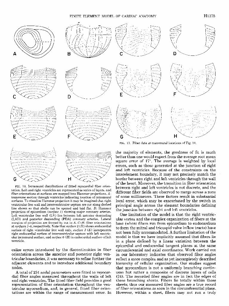
The distributions of fiber orientations in the three- * dimensional geometric model are shown in Fig. IO. The right ventricle is represented as a single shell continuous with the outer layer of the free wall of the left ventricle, and the interventricular septum is divided into three layers. The fiber field at each of the surfaces (Fig. IOA) has been mapped into a Hammer projection (20). To visualize this projection, imagine that a transmural cut is made from base to apex through the center of both the right ventricle and the interventricular septum and that each shell is then laid flat. The Hammer projection preserves relative surface area and retains the apex as a single point. Although this transformation imposes some spatial distortion on the fiber field, it is relatively simple to interpret and demonstrates qualitative differences in fiber orientation from apex to base between the anterior and posterior aspects of the left ventricle and between the left ventricular free wall and septum.

To provide landmarks, the approximate location of epicardial coronary arteries are superimposed on the


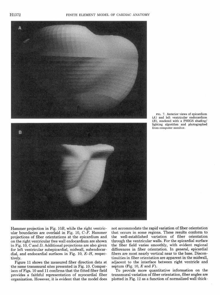
FIG. 7. Anterior views of eF (A) and left ventricular end (B), rendered with a PHIGS lighting algorithm and phot from computer monitor.

jicardium ocardium shading/

.ographed

Hammer projection in Fig. lOB, while the right ventricular boundaries are overlaid in Fig. 10, C-F. Hammer projections of fiber orientations at the epicardium and on the right ventricular free wall endocardium are shown in Fig. 10, C and D. Additional projections are also given for left ventricular subepicardial, midwall, subendocardial, and endocardial surfaces in Fig. 10, E-H, respectively.

Figure 11 shows the measured fiber direction data at the same transmural sites presented in Fig. 10. Compar- ison of Figs. 10 and 11 confirms that the fitted fiber field provides a faithful representation of myocardial fiber organization. However, it is evident that the model does

not accommodate the rapid variation of fiber orientation that occurs in some regions. These results conform to the well-established variation of fiber orientation through the ventricular walls. For the epicardial surface the fiber field varies smoothly, with evident regional differences in fiber orientation. In general, epicardial fibers are most nearly vertical near to the base. Discon- tinuities in fiber orientation are apparent in the midwall, adjacent to the interface between right ventricle and septum (Fig. 10, E and F).

To provide more quantitative information on the transmural variation of fiber orientation, fiber angles are plotted in Fig. 12 as a function of normalized wall thick-


c Q x - -5.0

4

Q

x = 5.0

X = 25.0

x = 35.0

)

0

x = 0.0

a trr:? x = 20.0

x = 30.0

x = 40.0

FIG. 8. Ventricular cross sections from finite element model at various axial locations (values given are in mm; 0 mm represents equatorial plane).

ness. In Fig. 12, A-F, distributions of fitted fiber angles in the right ventricular free wall are presented, together with surrounding data, for the sites indicated at the top of the figure. In addition, in Fig. 12, A and B, we have superimposed comparable data from Streeter et al. (29) for similar transmural sites. The extent of transmural fiber angle variation is greatest in the interventricular septum and is least for the free wall of the right ventricle. For the left ventricular free wall, the transmural variation of fiber angle is sigmoidal at equatorial sites (Fig. 12, A, C, and D) and relatively linear at a more apical site (Fig. 12B). This trend is a consistent feature of our data and indicates that the proportion of circumferentially orientated fibers is greater toward the base.

All figures presented relate to a single heart in which coordinate measurements were made at 576 points on the epicardium and at 360 and 403 points, respectively, on the left and right ventricular endocardial surfaces.

Myocardial fiber orientations were estimated at 8,690 points?

DISCUSSION

The techniques of continuum mechanics may be used to study many aspects of cardiac function. Particular examples include finite element analysis of ventricular stress and deformation (2, 11, 33) and the modeling of cardiac electrical activation (11,19). However, to employ this approach effectively, it is first necessary to imple- ment a realistic mathematical description of the three- dimensional geometry of the ventricles (17, 31). An accurate representation of ventricular muscle fiber organization is also required, since many of the physical properties of myocardium are dependent on local fiber orientation (22, 34). Finally, any such description of structure must be as compact as possible to ensure efficient solution of problems based on it. We have developed a finite element model that meets these requirements and provides, for the first time, a comprehensive and quantitative description of ventricular architecture.

In formulating this model we have employed the well- established finite element technique of approximating multidimensional fields using piecewise polynomials (35). Interpolation parameters, defined at each element node, have been fitted to detailed measurements of ventricular geometry and myocardial fiber orientation. Be- cause the finite element ensembles are referred to a coordinate system that closely matches ventricular boundary geometry, the mathematical description of structure is highly efficient. A further advantage of this representation is that parameters can be efficiently fitted using linear least-squares procedures.

The essential features of the model are as follows. 1) A prolate spheroid coordinate system is used to

represent the geometry. This leads to an efficient mathematical description because only X, the radial coordinate, requires a high-order basis. The remaining two angular coordinates, p and 0, are interpolated linearly. Another advantage of the prolate spheroidal model is that it provides a set of normalized coordinates with a single dimensional scaling factor, the focus distance a. This allows the geometry of hearts of different sizes to be compared readily.

2) The radial coordinate X is interpolated with bicubic Hermite basis functions in the surface coordinates & and &. The Hermite basis provides first-order derivative continuity of the X-coordinate, which means that few elements are needed to describe the endocardial and epicardial surfaces of the ventricles.

3) The fiber orientation field is described in the model by assuming that fibers lie in (&, &J-coordinate planes (which at one extreme form the epicardial surface and at the other the endocardial surface). The orientation of fibers with respect to the circumferential direction in these planes is described by a bilinear interpolation of nodal parameters, and the transmural variation of fiber angle has a cubic Hermite basis.

’ Copies of the raw data together with the sets of fitted parameters for both geometry and fiber angle fields are available on request from

P. J. Hunter (please enclose a Macintosh 3.5in. high-density disk).


Detailed descriptions of left and right ventricular geometry have been presented by Janicki et al. (12) and McLean and Prothero (15). However, these investigators made little attempt to compress their extensive data sets and did not present them in a parametric form directly amenable to modeling applications. In the present study we have demonstrated that relatively few elements are required to represent epicardial and endocardial surface geometry. A total of 164 nodal parameters have been fitted to the geometric data sets. This representation describes epicardial surface geometry with considerable accuracy and faithfully reproduces the important structural features of the endocardial surfaces of right and left ventricles.

Although there have been numerous studies of the transmural variation of ventricular muscle fiber orientation (1, 6, 9, 23, 28, 29), these have typically been restricted to relatively small numbers of measurement sites. One systematic approach explored by Nielsen (17) and by McLean and Prothero (15) is to cut right and left ventricles into thick serial slices transverse to the base- apex axis. Each slice is subdivided into wedges that are sectioned at transmural intervals using standard histo- logical procedures, and the distribution of fiber orientations across each wedge is determined from the serial sections. Detailed characterization of fiber distribution in this way clearly involves a daunting amount of work, which probably accounts for the present lack of comprehensive data. Moreover, conventional sectioning methods present a number of further problems. Tissue preparation and sectioning inevitably involves some distortion, which may introduce errors in spatial registration. To measure fiber orientation it is customary to section in a plane tangential to the epicardial surface, but in regions of rapidly varying curvature, this may be difficult to achieve. Finally, because of the complexity of fiber branching, it is usually advisable to average fiber orientation over a substantial section area, which limits the number of transmural sites at which the distribution of fiber orientation can be determined. More recently, McLean et al. (16) traced projected fiber paths in transverse and longitudinal planes. However, this approach cannot be used for precise three-dimensional reconstruc-

FIG. 9. Myocardial fiber orientation vectors at epicardium (A) and endocardial surface (B ) of left ventricle shown on corresponding Sdimensional finite element surface meshes. Only anterior views are given.

tion of cardiac muscle fiber orientation. Our technique of removing fine layers of myocardium

from an intact preparation overcomes many of the problems associated with conventional sectioning methods. At a given transmural depth it is possible to sample fiber orientations at large numbers of sites, and because the absolute coordinates of each site are monitored, spatial registration is implicitly preserved. A further advantage in sampling from a complete surface is that local fiber orientations may be determined with reference to the surrounding myocardium. Our technique is also relatively efficient, enabling comprehensive measurements of fiber orientation to be made throughout the myocardium. Nonetheless, the exhaustive mapping of fiber orientation reported here required many days of measurement.

The resolution of our measurement system is adequate for the present purpose. However, there are aspects of the mechanical design that could be improved. For instance, when making measurements from casts of the endocardial surface, it was sometimes not possible to advance the pointer into the concave regions associated with papillary muscles. Also, in estimating fiber orientation from the shadow cast on the myocardial surface, increasing uncertainty is introduced as the angle between the pointer and the surface tangent plane is reduced. It can be demonstrated that neither of these factors introduced systematic or substantial errors. Nevertheless, it would be possible to overcome these problems by rede- signing the measurement system so that the pointer could be oriented with respect to local material coordinates.

The model outlined here provides a very accurate representation of epicardial surface geometry and reproduces the most important features of the endocardial surfaces. Our analysis of fitting error indicates that the 24-bicubic element mesh used for this model is optimal in that it provides accuracy consistent with the measurement error for the least number of degrees of freedom.

When fitting fiber orientation data, the finite element mesh used for geometric fitting was refined in the circumferential direction to accommodate the observed variation in fiber orientation. Moreover. to reduce and lo-

FINITE ELEMENT MODEL OF CARDIAC ANATOMY

.

HI375

FIG. 10. Intramural distributions of fitted myocardial fiber orientation. Left and right ventricles are represented as series of layers, and fiber orientations at surfaces are mapped into Hammer projections. A: transverse section through ventricles indicating location of intramural surfaces. To visualize Hammer projection it may be imagined that right ventricular free wall and interventricular septum are cut along dashed line shown so that shells can be opened and laid flat. B: Hammer projection of epicardium (surface 1) showing major coronary arteries. Left ventricular free wall (LV) lies between left anterior descending (LAD) and posterior descending (PDA) coronary arteries. Lateral margins of projection are formed by cut in A. C-H: fiber orientations at surfaces l-6, respectively. Note that surface 2 (D) shows endocardial surface of right ventricular free wall only, surface 3 (E) incorporates right endocardial surface of interventricular septum with left ventricular intramural surface, and surface 6 (H) is endocardial surface of left ventricle.

calize errors introduced by the discontinuities in fiber orientation across the anterior and posterior right ventricular boundaries, it was necessary to refine further the adjacent elements and to introduce additional boundary nodes.

A total of 234 nodal parameters were fitted to myocardial fiber angles measured throughout the walls of left and right ventricles. The fitted fiber field provides a good representation of fiber orientation throughout the ventricular myocardium, and, in general, fitted fiber orientations are within the range of measurement error. In

FIG. 11. Fiber data at transmural locations of Fig. 10.

the majority of elements, the goodness of fit is much better than one would expect from the average root mean square error of 17”. The average is weighted by local errors, such as those generated at the junction of right and left ventricles. Because of the constraints on the interelement boundary, it may not precisely match the border between right and left ventricles through the wall of the heart. Moreover, the transition in fiber orientation between right and left ventricles is not discrete, and the different fiber fields are observed to merge across a zone of some millimeters. These factors result in substantial local error, which may be exacerbated by the switch in principal angle across the element boundaries defining the junction between right and left ventricles.

One limitation of the model is that the right ventricular vortex and the complex organization of fibers at the base (where fibers run from epicardium to endocardium to form the mitral and tricuspid valve inflow tracts) have not been fully accommodated. A further limitation of the model is that we have implicitly assumed that fibers lie in a plane defined by a linear variation between the epicardial and endocardial tangent planes at the same circumferential and axial coordinates. Work carried out in our laboratory indicates that observed fiber angles reflect a more complex and as yet incompletely described hierarchy of cellular organization. Our studies suggest that myocardium is not a uniformly branching continuum but rather a composite of discrete layers of cells (24). The recorded fiber angles are in fact the edges of these branching sheets. Fibers lie totally within these sheets; thus our measured fiber angles are a true record of fiber orientations as seen in the circumferential plane. However, within a sheet, fibers may not run a truly


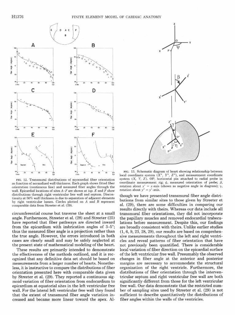
P

FIG. 12. Transmural distributions of myocardial fiber orientation as function of normalized wall thickness. Each graph shows fitted fiber orientation (continuous line) and measured fiber angles through the wall. Epicardial locations of sites A-F are shown at top. E and F show distributions through right ventricular free wall and septum. Discon- tinuity at 50% wall thickness is due to separation of adjacent elements by right ventricular lumen. Circles plotted on A and B represent comparable data from Streeter et al. (29).

circumferential course but traverse the sheet at a small angle. Furthermore, Streeter et al. (28) and Streeter (25) have reported that fiber pathways are directed inward from the epicardium with imbrication angles of 3-5”; thus the measured fiber angle is a projection rather than the true angle. However, the errors introduced in both cases are clearly small and may be safely neglected at the present state of mathematical modeling of the heart.

These results are primarily intended to demonstrate the effectiveness of the methods outlined, and it is rec- ognized that any definitive data set should be based on measurements from a larger number of hearts. Nonethe- less, it is instructive to compare the distributions of fiber orientation presented here with comparable data given by Streeter et al. (29). They reported a continuous sig- moid variation of fiber orientation from endocardium to epicardium at equatorial sites in the left ventricular free wall. For the lateral left ventricular free wall they found that the extent of transmural fiber angle variation in- creased and became more linear toward the apex. Al-

FIG. 13. Schematic diagram of heart showing relationship between local coordinate system (X”, Y”, Z”), and measurement coordinate system (X, Y, 2). OP, horizontal pin attached to radial probe in coordinate measurement rig; #, measured orientation of probe; p, rotation about x’ = x-axis (shown as negative angle in diagram); y, rotation about y” = y’-axis.

though we have presented transmural fiber angle distributions from similar sites to those given by Streeter et al. (29), there are some difficulties in comparing our results directly with theirs. Whereas our data include all transmural fiber orientations, they did not incorporate the papillary muscles and removed endocardial trabecu- lations before measurement. Despite this, our findings are broadly consistent with theirs. Unlike earlier studies (1, 6, 9, 23, 28, 29), our results are based on comprehensive measurements throughout the left and right ventricles and reveal patterns of fiber orientation that have not previously been quantified. There is considerable local variation of fiber direction on the epicardial surface of the left ventricular free wall. Presumably the observed changes in fiber angle at the anterior and posterior margins are necessary to accommodate the structural organization of the right ventricle. Furthermore, the distributions of fiber orientation through the interventricular septum and right ventricular free wall are both significantly different from those for the left ventricular free wall. Our data demonstrate that the restricted number of sampling sites used by Streeter et al. (29) is not sufficient to describe quantitatively the distributions of fiber angles within the walls of the ventricles.

FINITE ELEMENT MODEL

In conclusion, we have developed a finite element model that provides a compact and realistic mathematical representation of the geometry and fibrous organization of the right and left ventricles. We have also implemented specialized measurement techniques to obtain the anatomic data necessary to set up the model. These methods have yielded a more comprehensive and quantitative representation of ventricular structure than has previously been available, and at present we are extending the study to establish a representative description of canine ventricular architecture. The main objective of the work has been to support continuum mechanics analyses of various aspects of cardiac function. How- ever, the finite element model has also proved useful for displaying and analyzing potential fields measured on the epicardium during cardiac excitation where detailed information on ventricular geometry and fiber orientation is required.

APPENDIX

Fiber Angle Correction

In Fig. 13, OP represents the horizontal pin attached to the radial probe in the coordinate measurement rig. The probe is rotated about its axis until the shadow of the pin on the myocardial surface is aligned with the local fiber direction. To estimate the fiber angle q from +, the measured orientation of the probe about its axis, we assume that the fibers lie in the plane tangential to the point of probe contact 0”. The local coordinate system (X”, Y”, 2”) has 2” orthogonal to the tangent plane, and 0”P” is the projection of the pin in this plane. In the local coordinate system, the coordinates of P” are (x”, y”, 0) and the fiber angle 31 is given by

cot?j YN =- XN

(Al)

The relationship between the local coordinate system (X”, Y”, 2”) and the measurement coordinate system (X, Y, 2) is represented in Fig. 13. The coordinate transformation is illus- trated as a rotation y about the Y”-axis into the coordinate system (X’, Y’, 2’) followed by a rotation ,B about the XI-axis. The transformation matrix is

X

[I [

cosy 0 siny XII

Y = -sin@iny co@ sin@cosy

z -cos@iny -sir@ cospcosy IL 1 y” 2”

Therefore

Y = OPcos$ = y”co@ - x”sin@iny

X = OPsin# = XNcos~

and from Eqs. Al and A2

bw

cotq cosy

= - cot+ + sinytanp cosp

W)

The angles ,8 and y, which specify the orientation of the surface with respect to the measurement coordinate system, are derived from adjacent data points and used in Eq. A3 to estimate the fiber angle.

We gratefully acknowledge the expert technical assistance of Joan Ready, Tian Xin, and Martin Garrett; the PHIGS graphical program-

OF CARDIAC ANATOMY H1377

ming assistance of Alistair Young; and the skilled artwork of Arthur Ellis.

This work was supported by project grants from the Life Insurance Medical Research Foundation of Australia and New Zealand and the National Heart Foundation of New Zealand. I. Le Grice is funded by the Auckland Medical Research Foundation.

Address for reprint requests: P. J. Hunter, Dept. of Engineering Science, School of Engineering, Univ. of Aukland, Private Bag, Auk- land, New Zealand.

Received 15 May 1989; accepted in final form 19 November 1990.

REFERENCES

1.

2.

3.

4.

5.

6.

7.

8.

9.

10.

11.

12.

13.

14.

15.

16.

17.

18.

19.

ARMOUR, J. A., AND W. C. RANDALL. Structural basis for cardiac function. Am. J. Physiol. 218: 1517-1523, 1970.

BERGEL, D. A., AND P. J. HUNTER. Mechanics of the heart. In: Quantitative Cardiovascular Studies: Clinical and Research Appli- cations of Engineering Principles, edited by N. H. C. Wang, D. R. Gross, and D. J. Patel. Baltimore, MD: University Park, 1979, p. 151-213.

CHANG, S. K., AND C. K. CHOW. The reconstruction of three- dimensional objects from two orthogonal projections and its appli- cation to cardiac cineangiography. IEEE Trans. Comput. 22: 18- 25, 1973. DIEUDONNE, J. M. The left ventricle as confocal spheroids. BULL. Math. Biophys. 31: 433-439, 1969. FALSETTI, H. L., R. E. MATES, C. GRANT, D. G. GREEN, AND I. L. BUNNELL. Left ventricular wall stress calculated from one-plane cineangiography: an approach to force-velocity analysis in man. Circ. Res. 26: 71-83, 1970. FOX, C. C., AND G. M. HUTCHINS. The architecture of the human ventricular myocardium. Johns Hopkins Med. J. 130: 289-299, 1972. GEISER, E. A., S. M. LUPKIEWICZ, L. G. CHRISTIE, M. ARIET, D. A. CONETTA, AND C. R. CONTI. A framework for three-dimensional time-varying reconstruction of the human left ventricle: sources of error and estimation of their magnitude. Comput. Biomed. Res. 13: 225-241, 1980. GOULD, P., D. GHISTA, L. BROMBOLICH, AND I. MIRSKY. In vivo stresses in the human left ventricular wall: analysis accounting for the irregular 3dimensional geometry and comparison with ideal- ised geometry analyses. J. Biomech. 5: 521-539, 1972. GREENBAUM, R. A., S. Y. Ho, D. G. GIBSON, A. E. BECKER, AND

R. H. ANDERSON. Left ventricular fibre architecture in man. Br. Heart J. 45: 248-263, 1981. HUNTER, P. J., A. D. MCCULLOCH, P. M. F. NEILSEN, AND B. H. SMAILL. A finite element model of passive ventricular mechanics. In: Computational Methods in Bioengineering, edited by R. L. Spilker and B. R. Simon. New York: Am. Sot. Mech. Eng., 1988, vol. 9, p. 387-397. HUNTER, P. J., AND B. H. SMAILL. The analysis of cardiac function: a continuum approach. Prog. Biophys. Mol. Biol. 52: lOl-164,1989. JANICKI, J. S., K. T. WEBER, R. F. GOCHMAN, S. SHROFF, AND F. J. GEHEB. Three-dimensional myocardial and ventricular shape: a surface representation. Am. J. Physiol. 241 (Heart Circ. Physiol. 10): Hl-Hll, 1981. MACCALLUM, J. B. On the muscular architecture and growth of the ventricles of the heart. Johns Hopkins Hosp. Rep. 9: 307-335, 1900. MALL, F. P. On the muscular architecture of the ventricles of the human heart. Am. J. Anat. 11: Zll-266,191l. MCLEAN, M. R., AND J. PROTHERO. Coordinated three-dimensional reconstruction from serial sections at macroscopic and mi- croscopic levels of resolution; the human heart. Anat. Rec. 219: 434-439,1987. MCLEAN, M., M. A. Ross, AND J. PROTHERO. Three-dimensional reconstruction of the myofiber pattern in the fetal and neonatal mouse heart. Anat. Rec. 224: 392-406, 1989. NIELSEN, P. M. F. The Anatomy of the Heart: A Finite Element ModeZ (PhD thesis). Auckland, New Zealand: Univ. of Auckland, 1987. PAO, Y. C., E. L. RITMAN, AND E. H. WOOD. Finite-element analysis of left ventricular myocardial stresses. J. Biomech. 7: 469- 477, 1974. PLONSEY, R., AND R. C. BARR. Mathematical modeling of electrical


20. 21.

22.

23.

24.

25.

26.

27.

activity of the heart. J. Electrocardiol. 20: 219-226, 1987. RAISZ, E. Principles of Cartography. New York: McGraw-Hill, 1962. RITMAN, E. L., J. H. KINSEY, R. A. ROBB, B. K. GILBERT, L. D. HARRIS, AND E. H. WOOD. Three-dimensional imaging of heart, lungs, and circulation. Science Wash. DC 210: 273-280, 1980. ROBERTS, D. E., L. T. HERSH, AND A. M. SCHER. Influence of cardiac fiber orientation on wavefront voltage, conduction velocity, and tissue resistivity in the dog. Circ. Res. 44: 701-712, 1979. Ross, M. A., AND D. D. STREETER, JR. Nonuniform subendocardial fiber orientation in the normal macaque left ventricle. Eur. J. Cardiol. 3: 229-247, 1975. SMAILL, B. H., AND P. J. HUNTER. Structure and function of the diastolic heart: material properties of the passive myocardium. In: Theory of the Heart, edited by L. Glass, P. J. Hunter, and A. D. McCulloch. New York: Springer-Verlag. In press. STREETER, D. .D., JR. Gross morphology and fiber geometry of the heart. In: Handbook of Physiology. The Cardiovascular System. Bethesda, MD: Am. Physiol. Sot., 1979, sect. 2, vol. I, chapt. 4, p. 61-112. STREETER, D. D., JR., AND D. L. BASSETT. An engineering analysis of myocardial fiber orientation in pig’s left ventricle in systole. Anat. Rec. 155: 503-511, 1966. STREETER, D. D., JR., AND W. T. HANNA. Engineering mechanics for successive states in canine left ventricular myocardium. 1.

Cavity and wall geometry. Circ. Res. 33: 639-655, 1973. 28. STREETER, D. D., JR., W. E. POWERS, M. A. Ross, AND F.

TORRENT-GUASP. Three-dimensional fiber orientation in the mammalian left ventricular wall. In: Cardiovascular System Dy- namics, edited by J. Baan, A. Noordergraaf, and J. Raines. Cam- bridge, MA: MIT, 1978, p. 73-84.

29. STREETER, D. D., JR., H. M. SPOTNITZ, D. P. PATEL, J. Ross, JR., AND E. H. SONNENBLICK. Fiber orientation in the canine left ventricle during diastole and systole. Circ. Res. 24: 339-347, 1969.

30. WRIGHT, R. L., S. LEVITSKY, C. HOLLAND, AND H. FEINBURG.

Beneficial effects of potassium cardioplegia during intermittent aortic cross-clamping and reperfusion. J. Surg. Res. 24: 201-209, 1978.

31. YETTRAM, A. L., AND C. A. VINSON. Geometric modelling of the human left ventricle. J. Biomech. Eng. 101: 221-223, 1979.

32. YETTRAM, A. L., C. A. VINSON, AND D. G. GIBSON. Computer modelling of the human left ventricle. J. Biomech. Eng. 104: 148- 152, 1982.

33. YIN, F. C. P. Ventricular wall stress. Circ. Res. 49: 829-842, 1981. 34. YIN, F. C. P., R. K. STRUMPF, P. H. CHEW, AND S. L. ZEGER.

Quantification of the mechanical properties of non-contracting canine myocardium. J. Biomech. 20: 577-589, 1987.

35. ZIENKIEWICZ, 0. C., AND K. MORGAN. Finite Elements and Ap- proximation. New York: Wiley, 1982.

Mathematical model of geometry and fibrous structure of the heart

Documents