Mathematical Methods of Engineering Analysis Erhan C ¸ inlar Robert J. Vanderbei February 2, 2000

Welcome message from author
This document is posted to help you gain knowledge. Please leave a comment to let me know what you think about it! Share it to your friends and learn new things together.
Transcript

Mathematical Methods of Engineering Analysis
Erhan Cinlar Robert J. Vanderbei
February 2, 2000

Contents
Sets and Functions 11 Sets . . . . . . . . . . . . . . . . . . . . . . . . . . . . . . . . . . . 1
Subsets . . . . . . . . . . . . . . . . . . . . . . . . . . . . . 2Set Operations . . . . . . . . . . . . . . . . . . . . . . . . . 2Disjoint Sets . . . . . . . . . . . . . . . . . . . . . . . . . . 3Products of Sets . . . . . . . . . . . . . . . . . . . . . . . . 3
2 Functions and Sequences . . . . . . . . . . . . . . . . . . . . . . . . 4Injections, Surjections, Bijections . . . . . . . . . . . . . . . 4Sequences . . . . . . . . . . . . . . . . . . . . . . . . . . . . 5
3 Countability . . . . . . . . . . . . . . . . . . . . . . . . . . . . . . . 64 On the Real Line . . . . . . . . . . . . . . . . . . . . . . . . . . . . 8
Positive and Negative . . . . . . . . . . . . . . . . . . . . . . 9Increasing, Decreasing . . . . . . . . . . . . . . . . . . . . . 9Bounds . . . . . . . . . . . . . . . . . . . . . . . . . . . . . 9Supremum and Infimum . . . . . . . . . . . . . . . . . . . . 9Limits . . . . . . . . . . . . . . . . . . . . . . . . . . . . . . 10Convergence of Sequences . . . . . . . . . . . . . . . . . . . 11
5 Series . . . . . . . . . . . . . . . . . . . . . . . . . . . . . . . . . . 14Ratio Test, Root Test . . . . . . . . . . . . . . . . . . . . . . 16Power Series . . . . . . . . . . . . . . . . . . . . . . . . . . 17Absolute Convergence . . . . . . . . . . . . . . . . . . . . . 18Rearrangements . . . . . . . . . . . . . . . . . . . . . . . . . 19
Metric Spaces 236 Euclidean Spaces . . . . . . . . . . . . . . . . . . . . . . . . . . . . 23
Inner Product and Norm . . . . . . . . . . . . . . . . . . . . 23Euclidean Distance . . . . . . . . . . . . . . . . . . . . . . . 24
7 Metric Spaces . . . . . . . . . . . . . . . . . . . . . . . . . . . . . . 25Usage . . . . . . . . . . . . . . . . . . . . . . . . . . . . . . 26Distances from Points to Sets and from Sets to Sets . . . . . . 26Balls . . . . . . . . . . . . . . . . . . . . . . . . . . . . . . 26
8 Open and Closed Sets . . . . . . . . . . . . . . . . . . . . . . . . . . 29Closed Sets . . . . . . . . . . . . . . . . . . . . . . . . . . . 30Interior, Closure, and Boundary . . . . . . . . . . . . . . . . 30
i

Open Subsets of the Real Line . . . . . . . . . . . . . . . . . 319 Convergence . . . . . . . . . . . . . . . . . . . . . . . . . . . . . . 34
Subsequences . . . . . . . . . . . . . . . . . . . . . . . . . . 35Convergence and Closed Sets . . . . . . . . . . . . . . . . . 36
10 Completeness . . . . . . . . . . . . . . . . . . . . . . . . . . . . . . 37Cauchy Sequences . . . . . . . . . . . . . . . . . . . . . . . 37Complete Metric Spaces . . . . . . . . . . . . . . . . . . . . 38
11 Compactness . . . . . . . . . . . . . . . . . . . . . . . . . . . . . . 40Compact Subspaces . . . . . . . . . . . . . . . . . . . . . . 40Cluster Points, Convergence, Completeness . . . . . . . . . . 41Compactness in Euclidean Spaces . . . . . . . . . . . . . . . 42
Functions on Metric Spaces 4512 Continuous Mappings . . . . . . . . . . . . . . . . . . . . . . . . . . 45
Continuity and Open Sets . . . . . . . . . . . . . . . . . . . 46Continuity and Convergence . . . . . . . . . . . . . . . . . . 46Compositions . . . . . . . . . . . . . . . . . . . . . . . . . . 47Real-Valued Functions . . . . . . . . . . . . . . . . . . . . . 48Rn-Valued Functions . . . . . . . . . . . . . . . . . . . . . . 48
13 Compactness and Uniform Continuity . . . . . . . . . . . . . . . . . 50Uniform Continuity . . . . . . . . . . . . . . . . . . . . . . . 51
14 Sequences of Functions . . . . . . . . . . . . . . . . . . . . . . . . . 53Cauchy Criterion . . . . . . . . . . . . . . . . . . . . . . . . 54Continuity of Limit Functions . . . . . . . . . . . . . . . . . 56
15 Spaces of Continuous Functions . . . . . . . . . . . . . . . . . . . . 57Convergence inC . . . . . . . . . . . . . . . . . . . . . . . . 57Lipschitz Continuous Functions . . . . . . . . . . . . . . . . 58Completeness . . . . . . . . . . . . . . . . . . . . . . . . . . 60Functionals . . . . . . . . . . . . . . . . . . . . . . . . . . . 60
Differential and Integral Equations 6316 Contraction Mappings . . . . . . . . . . . . . . . . . . . . . . . . . 63
Fixed Point Theorem . . . . . . . . . . . . . . . . . . . . . . 6417 Systems of Linear Equations . . . . . . . . . . . . . . . . . . . . . . 69
Maximum Norm . . . . . . . . . . . . . . . . . . . . . . . . 69Manhattan Metric . . . . . . . . . . . . . . . . . . . . . . . . 70Euclidean Metric . . . . . . . . . . . . . . . . . . . . . . . . 70Conclusion . . . . . . . . . . . . . . . . . . . . . . . . . . . 71
18 Integral Equations . . . . . . . . . . . . . . . . . . . . . . . . . . . . 71Fredholm Equation . . . . . . . . . . . . . . . . . . . . . . . 71Volterra Equation . . . . . . . . . . . . . . . . . . . . . . . . 76Generalization of the Fixed Point Theorem . . . . . . . . . . 77
19 Differential Equations . . . . . . . . . . . . . . . . . . . . . . . . . . 78
ii
Convex Analysis 8320 Convex Sets and Convex Functions . . . . . . . . . . . . . . . . . . . 8321 Projection . . . . . . . . . . . . . . . . . . . . . . . . . . . . . . . . 8622 Supporting Hyperplane Theorem . . . . . . . . . . . . . . . . . . . . 90
Measure and Integration 9123 Motivation . . . . . . . . . . . . . . . . . . . . . . . . . . . . . . . . 9124 Algebras . . . . . . . . . . . . . . . . . . . . . . . . . . . . . . . . . 93
Monotone Class Theorem . . . . . . . . . . . . . . . . . . . 9425 Measurable Spaces and Functions . . . . . . . . . . . . . . . . . . . 96
Measurable Functions . . . . . . . . . . . . . . . . . . . . . 96Borel Functions . . . . . . . . . . . . . . . . . . . . . . . . . 97Compositions of Functions . . . . . . . . . . . . . . . . . . . 97Numerical Functions . . . . . . . . . . . . . . . . . . . . . . 97Positive and Negative Parts of a Function . . . . . . . . . . . 98Indicators and Simple Functions . . . . . . . . . . . . . . . . 98Approximations by Simple Functions . . . . . . . . . . . . . 99Limits of Sequences of Functions . . . . . . . . . . . . . . . 100Monotone Classes of Functions . . . . . . . . . . . . . . . . 100Notation . . . . . . . . . . . . . . . . . . . . . . . . . . . . 101
26 Measures . . . . . . . . . . . . . . . . . . . . . . . . . . . . . . . . 103Arithmetic of Measures . . . . . . . . . . . . . . . . . . . . . 104Finite,σ-finite, Σ-finite measures . . . . . . . . . . . . . . . 104Specification of Measures . . . . . . . . . . . . . . . . . . . 105Image of Measure . . . . . . . . . . . . . . . . . . . . . . . 106Almost Everywhere . . . . . . . . . . . . . . . . . . . . . . 106
27 Integration . . . . . . . . . . . . . . . . . . . . . . . . . . . . . . . . 108Definition of the Integral . . . . . . . . . . . . . . . . . . . . 109Integral over a Set . . . . . . . . . . . . . . . . . . . . . . . 110Integrability . . . . . . . . . . . . . . . . . . . . . . . . . . . 110Elementary Properties . . . . . . . . . . . . . . . . . . . . . 110Monotone Convergence Theorem . . . . . . . . . . . . . . . 111Linearity of Integration . . . . . . . . . . . . . . . . . . . . . 113Fatou’s Lemma . . . . . . . . . . . . . . . . . . . . . . . . . 113Dominated Convergence Theorem . . . . . . . . . . . . . . . 114
iii

Sets and Functions
This introductory chapter is devoted to general notions regarding sets, functions, se-quences, and series. The aim is to introduce and review the basic notation, terminology,conventions, and elementary facts.
1 Sets
A setis a collection of some objects. Given a set, the objects that form it are called itselements. Given a setA, we writex ∈ A to mean thatx is an element ofA. To say thatx ∈ A, we also use phrases likex is in A, x is a member ofA, x belongs toA, andAincludesx.
To specify a set, one can either write down all its elements inside curly brackets (ifthis is feasible), or indicate the properties that distinguish its elements. For example,A = {a, b, c} is the set whose elements area, b, andc, andB = {x : x > 2.7} is theset of all numbers exceeding2.7. The following are some special sets:
∅: Theempty set. It has no elements.
N = {1, 2, 3, . . .}: Set ofnatural numbers.
Z = {0, 1,−1, 2,−2, . . .}: Set ofintegers.
Z+ = {0, 1, 2, . . .}: Set ofpositive integers.
Q = {mn : m ∈ Z, n ∈ N}: Set ofrationals.
R = (−∞,∞) = {x : −∞ < x < +∞}: Set ofreals.
[a, b] = {x ∈ R : a ≤ x ≤ b}: Closed intervals.
(a, b) = {x ∈ R : a < x < b}: Open intervals.
R+ = [0,∞) = {x ∈ R : x ≥ 0}: Set ofpositive reals.
1

2 SETS AND FUNCTIONS
Subsets
A setA is said to be asubsetof a setB if every element ofA is an element ofB. Wewrite A ⊂ B or B ⊃ A to indicate it and use expressions likeA is contained inB,B containsA, to the same effect. The setsA andB are the same, and then we writeA = B, if and only if A ⊂ B andA ⊃ B. We writeA 6= B whenA andB are not thesame. The setA is called aproper subsetof B if A is a subset ofB andA andB arenot the same.
The empty set is a subset of every set. This is a point of logic: letA be a set;the claim is that∅ ⊂ A, that is, that every element of∅ is also an element ofA,or equivalently, there is no element of∅ that does not belong toA. But the last isobviously true simply because∅ has no elements.
Set Operations
LetA andB be sets. Theirunion, denoted byA∪B, is the set consisting of all elementsthat belong to eitherA or B (or both). Theirintersection, denoted byA ∩ B, is theset of all elements that belong to bothA andB. Thecomplementof A in B, denotedby B \ A, is the set of all elements ofB that are not inA. Sometimes, whenB isunderstood from context,B \ A is also called the complement ofA and is denoted byAc. Regarding these operations, the following hold:
Commutative laws:
A ∪B = B ∪A,
A ∩B = B ∩A.
Associative laws:
(A ∪B) ∪ C = A ∪ (B ∪ C),(A ∩B) ∩ C = A ∩ (B ∩ C).
Distributive laws:
A ∩ (B ∪ C) = (A ∩B) ∪ (A ∩ C),A ∪ (B ∩ C) = (A ∪B) ∩ (A ∪ C).
The associative laws show thatA∪B∪C andA∩B∩C have unambiguous meanings.Definitions of unions and intersections can be extended to arbitrary collections of
sets. LetI be a set. For eachi ∈ I, let Ai be a set. Theunionof the setsAi, i ∈ I, isthe setA such thatx ∈ A if and only if x ∈ Ai for somei in I. The following notationsare used to denote the union and intersection respectively:⋃
i∈I
Ai,⋂i∈I
Ai.

1. SETS 3
WhenI = N = {1, 2, 3, . . .}, it is customary to write
∞⋃i=1
Ai,∞⋂
i=1
Ai.
All of these notations follow the conventions for sums of numbers. For instance,
n⋃i=1
Ai = A1 ∪ · · · ∪An,13⋂
i=5
Ai = A5 ∩A6 ∩ · · · ∩A13
stand, respectively, for the union overI = {1, . . . , n} and the intersection overI ={5, 6, . . . , 13}.
Disjoint Sets
Two sets are said to bedisjoint if their intersection is empty; that is, if they have noelements in common. A collection{Ai : i ∈ I} of sets is said to bedisjointedif Ai
andAj are disjoint for alli andj in I with i 6= j.
Products of Sets
Let A andB be sets. Theirproduct, denoted byA×B, is the set of all pairs(x, y) withx in A andy in B. It is also called therectanglewith sidesA andB.
If A1, . . . , An are sets, then their productA1 × · · · × An is the set of all n-tuples(x1, . . . , xn) wherex1 ∈ A1, . . . , xn ∈ An. This product is called, variously, a rect-angle, or a box, or an n-dimensional box. IfA1 = · · · = An = A, thenA1 × · · · ×An
is denoted byAn. Thus,R2 is the plane,R3 is the three-dimensional space,R2+ is the
positive quadrant of the plane, etc.
Exercises:1.1 Let E be a set. Show the following for subsetsA,B,C, andAi of E.
Here, all complements are with respect toE; for instance,Ac = E \A.
1. (Ac)c = A
2. B \A = B ∩Ac
3. (B \A) ∩ C = (B ∩ C) \ (A ∩ C)4. (A ∪B)c = Ac ∩Bc
5. (A ∩B)c = Ac ∪Bc
6. (⋃
i∈I Ai)c =⋂
i∈I Aci
7. (⋂
i∈I Ai)c =⋃
i∈I Aci
1.2 Leta andb be real numbers witha < b. Find∞⋃
n=1
[a +1n
, b− 1n
],∞⋂
n=1
[a− 1n
, b +1n
]

4 SETS AND FUNCTIONS
1.3 Describe the following sets in words and pictures:
1. A = {x ∈ R2 : x21 + x2
2 < 1}2. B = {x ∈ R2 : x2
1 + x22 ≤ 1}
3. C = B \A
4. D = C ×B
5. S = C × C
1.4 LetAn be the set of points(x, y) ∈ R2 lying on the curvey = 1/xn,0 < x < ∞. What is
⋂n≥1 An?
2 Functions and Sequences
Let E and F be sets. With each elementx of E, let there be associated a uniqueelementf(x) of F . Thenf is called afunctionfrom E into F , andf is said tomapEinto F . We writef : E 7→ F to indicate it.
Let f be a function fromE into F . For x in E, the pointf(x) in F is called theimageof x or the value off atx. Similarly, forA ⊂ E, the set
{y ∈ F : y = f(x) for somex ∈ A}
is called theimageof A. In particular, the image ofE is called therangeof f . Movingin the opposite direction, forB ⊂ F ,
f−1(B) = {x ∈ E : f(x) ∈ B}2.1
is called theinverse imageof B underf . Obviously, the inverse ofF is E.Terms like mapping, operator, transformation are synonyms for the term “function”
with varying shades of meaning depending on the context and on the setsE andF . Weshall become familiar with them in time. Sometimes, we writex 7→ f(x) to indicatethe mappingf ; for instance, the mappingx 7→ x3 + 5 from R into R is the functionf : R 7→ R defined byf(x) = x3 + 5.
Injections, Surjections, Bijections
Let f be a function fromE into F . It is called aninjection, or is said to beinjective, oris said to beone-to-one, if distinct points have distinct images (that is, ifx 6= y impliesf(x) 6= f(y)). It is called asurjection, or is said to besurjective, if its range isF ,in which casef is said to be fromE ontoF . It is called abijection, or is said to bebijective, if it is both injective and surjective.
These terms are relative toE andF . For examples,x 7→ ex is an injection fromRinto R, but is a bijection fromR into (0,∞). The functionx 7→ sinx from R into R isneither injective nor surjective, but it is a surjection fromR onto[−1, 1].

2. FUNCTIONS AND SEQUENCES 5
Sequences
A sequenceis a function fromN into some set. Iff is a sequence, it is custom-ary to denotef(n) by something likexn and write(xn) or (x1, x2, . . .) for the se-quence (instead off ). Then, thexn are called thetermsof the sequence. For instance,(1, 3, 4, 7, 11, . . .) is a sequence whose first, second, etc. terms arex1 = 1, x2 = 3, ....
If A is a set and every term of the sequence(xn) belongs toA, then(xn) is said tobe a sequence inA or a sequence of elements ofA, and we write(xn) ⊂ A to indicatethis.
A sequence(xn) is said to be asubsequenceof (yn) if there exist integers1 ≤k1 < k2 < k3 < · · · such that
xn = ykn
for eachn. For instance, the sequence(1, 1/2, 1/4, 1/8, . . .) is a subsequence of(1, 1/2, 1/3, 1/4, 1/5, . . .).
Exercises:
2.1 Letf be a mapping fromE into F . Show that
1. f−1(∅) = ∅,2. f−1(F ) = E,
3. f−1(B \ C) = f−1(B) \ f−1(C),
4. f−1(⋃
i∈I Bi) =⋃
i∈I f−1(Bi),
5. f−1(⋂
i∈I Bi) =⋂
i∈I f−1(Bi),
for all subsetsB,C,Bi of F .
2.2 Show thatx 7→ e−x is a bijection fromR+ onto (0, 1]. Show thatx 7→log x is a bijection from(0,∞) onto R. (Incidentally,log x is the loga-rithm of x to the basee, which is nowadays called the natural logarithm.We call it the logarithm. Let others call their logarithms “unnatural.”)
2.3 Letf be defined by the arrows below:
1 2 3 4 5 6 7 · · ·↓ ↓ ↓ ↓ ↓ ↓ ↓0 −1 1 −2 2 −3 3 · · ·
This defines a bijection fromN ontoZ. Using this, construct a bijectionfrom Z ontoN.
2.4 Letf : N×N 7→ N be defined by the table below wheref(i, j) is the entryin the ith row and thejth column. Use this and the preceding exercise toconstruct a bijection fromZ× Z ontoN.

6 SETS AND FUNCTIONS
... j 1 2 3 4 5 6 · · ·
i...
1 1 3 6 10 15 212 2 5 9 14 203 4 8 13 194 7 12 185 11 176 16...
2.5 Functional Inverses.Let f be a bijection fromE ontoF . Then, for eachy in F there is a uniquex in E such thatf(x) = y. In other words, inthe notation of (2.1),f−1({y}) = {x} for eachy in F and some uniquex in E. In this case, we drop some brackets and writef−1(y) = x. Theresulting functionf−1 is a bijection fromF ontoE; it is called the func-tional inverse off . This particular usage should not be confused with thegeneral notation off−1. (Note that (2.1) defines a functionf−1 form Finto E , whereF is the collection of all subsets ofF andE is the collectionof all subsets ofE.)
3 Countability
Two setsA andB are said to have the same cardinality, and then we writeA ∼ B, ifthere exists a bijection fromA ontoB. Obviously, having the same cardinality is anequivalence relation; it is
1. reflexive:A ∼ A,
2. symmetric:A ∼ B ⇒ B ∼ A,
3. transitive:A ∼ B andB ∼ C ⇒ A ∼ C.
A set is said to befinite if it is empty or has the same cardinality as{1, 2, . . . , n} forsomen in N; in the former case it has0 elements, in the latter exactlyn. It is said tobecountableif it is finite or has the same cardinality asN; in the latter case it is said tohave a countable infinity of elements.
In particular,N is countable. So areZ, N × N in view of exercises 2.3 and 2.4.Note that an infinite set can have the same cardinality as one of its proper subsets. Forinstance,Z ∼ N, R+ ∼ (0, 1], R ∼ R+ ∼ (0, 1); see exercise 2.2 for the latter.Incidentally,R+, R, etc. are uncountable, as we shall show shortly.
A set is countable if and only if it can be injected intoN, or equivalently, if andonly if there is a surjection fromN onto it. Thus, a setA is countable if and only ifthere is a sequence(xn) whose range isA. The following lemma follows easily fromthese remarks.

3. COUNTABILITY 7
3.1 LEMMA. If A can be injected intoB andB is countable, thenA is countable. IfA is countable and there is a surjection fromA ontoB, thenB is countable.
3.2 THEOREM.The product of two countable sets is countable.
PROOF. LetA andB be countable. If one of them is empty, thenA×B is empty andthere is nothing to prove. Suppose that neither is empty. Then, there exist injectionsf : A 7→ N andg : B 7→ N. For each pair(x, y) in A×B, let h(x, y) = (f(x), g(y));thenh is an injection fromA×B into N×N. SinceN×N is countable (see Exercise(2.4)), this implies via the preceding lemma thatA×B is countable 2
3.3 COROLLARY.The set of all rational numbers is countable.
PROOF. Recall that the setQ of all rationals consists of ratiosm/n with m ∈ Z andn ∈ N. Thus,f(m,n) = m/n defines a surjection fromZ×N ontoQ. SinceZ andNare countable, so isZ×N by the preceding theorem. Hence,Q is countable by Lemma3.1. 2
3.4 THEOREM.The union of a countable collection of countable sets is countable.
PROOF. LetI be a countable set, and letAi be a countable set for eachi in I. Theclaim is thatA =
⋃i∈I Ai is countable. Now, there is a surjectionfi : N 7→ Ai for
eachi, and there is a surjectiong : N 7→ I; these follow from the countability ofI andtheAi. Note that, then,h(m,n) = fg(m)(n) defines a surjectionh from N × N ontoA. SinceN× N is countable, this implies via Lemma 3.1 thatA is countable. 2
The following theorem exhibits an uncountable set. As a corollary, we show thatRis uncountable.
3.5 THEOREM.LetE be the set of all sequences whose terms are the digits0 and1.Then,E is uncountable.
PROOF. LetA be a countable subset ofE. Let x1, x2, . . . be an enumeration of theelements ofA, that is,A is the range of(xn). Note that eachxn is a sequence of zerosand ones, sayxn = (xn,1, xn,2, . . .) where each termxn,m is either0 or 1. We definea new sequencey = (yn) by lettingyn = 1− xn,n. The sequencey differs from everyone of the sequencesx1, x2, . . . in at least one position. Thus,y is not inA but is inE.
We have shown that ifA ⊂ E and is countable, then there is ay ∈ E such thaty 6∈ A. If E were countable, the preceding would hold forA = E, which would be

8 SETS AND FUNCTIONS
absurd. Hence,E must be uncountable. 2
3.6 COROLLARY.The set of all real numbers is uncountable.
PROOF. It is enough to show that the interval[0, 1) is uncountable. For eachx ∈ [0, 1),let 0.x1x2x3 · · · be the binary expansion ofx (in casex is dyadic, sayx = k/2n forsomek andn in N, there are two such possible binary expansions, in which case wetake the expansion with infinitely many zeros), and we identify the binary expansionwith the sequence(x1, x2, . . .) in the setE of the preceding theorem. Thus, to eachx in [0, 1) there corresponds a unique elementf(x) of E. In fact, f is a surjectiononto the setE \ D whereD denotes the set of all sequences of zeros and ones thatare eventually all ones. It is easy to show thatD is countable and hence thatE \D isuncountable. From this it follows that[0, 1) is uncountable. 2
Exercises:3.1 Dyadics.A number is said to be dyadic if it has the formk/2n for some in-
tegersk andn in Z+. Show that the set of all dyadic numbers is countable.Of course, every dyadic number is rational.
3.2 LetD denote the set of all sequences of zeros and ones that are eventuallyall ones. Show thatD is countable.
3.3 Suppose thatA is uncountable and thatB is countable. Show thatA \ Bis uncountable.
3.4 Letx be a real number. For eachn ∈ Z+, let xn be the smallest dyadicnumber of the formk/2n that exceedsx. Show thatx0 ≥ x1 ≥ x2 ≥ · · ·and thatxn > x for eachn. Show that, for everyε > 0, there is annε suchthatxn − x < ε for all n ≥ nε.
4 On the Real Line
The object is to review some facts and establish some terminology regarding the setR of all real numbers and the setR = [−∞,+∞] of all extended real numbers. Theextended real number systemconsists ofR and two extra symbols,−∞ and∞. Therelation< is extended toR by postulating that−∞ < x < +∞ for every real numberx. The arithmetic operations are extended toR as follows: for eachx ∈ R,
x +∞ = x− (−∞) = ∞x + (−∞) = x−∞ = −∞
x · ∞ ={
∞ if x > 0−∞ if x < 0
4. ON THE REAL LINE 9
x · (−∞) = (−x) · ∞x/∞ = x/(−∞) = 0
∞+∞ = ∞(−∞) + (−∞) = −∞
∞ ·∞ = (−∞) · (−∞) = ∞∞ · (−∞) = −∞.
The operations0 · (±∞), (−∞)− (−∞), +∞/+∞, and−∞/−∞ are undefined.
Positive and Negative
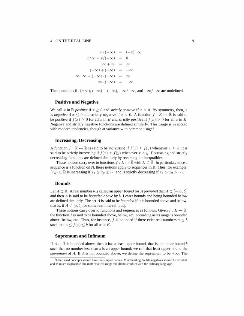
We callx in R positiveif x ≥ 0 andstrictly positiveif x > 0. By symmetry, then,xis negativeif x ≤ 0 and strictly negative ifx < 0. A function f : E 7→ R is said tobepositiveif f(x) ≥ 0 for all x in E andstrictly positiveif f(x) > 0 for all x in E.Negative and strictly negative functions are defined similarly. This usage is in accordwith modern tendencies, though at variance with common usage1.
Increasing, Decreasing
A function f : R 7→ R is said to beincreasingif f(x) ≤ f(y) wheneverx ≤ y. It issaid to bestrictly increasingif f(x) < f(y) wheneverx < y. Decreasing and strictlydecreasing functions are defined similarly by reversing the inequalities.
These notions carry over to functionsf : E 7→ R with E ⊂ R. In particular, since asequence is a function onN, these notions apply to sequences inR. Thus, for example,(xn) ⊂ R is increasing ifx1 ≤ x2 ≤ · · · and is strictly decreasing ifx1 > x2 > · · ·.
Bounds
LetA ⊂ R. A real numberb is called anupper boundfor A provided thatA ⊂ [−∞, b],and thenA is said to bebounded aboveby b. Lower bounds and being bounded beloware defined similarly. The setA is said to beboundedif it is bounded above and below;that is, ifA ⊂ [a, b] for some real interval[a, b].
These notions carry over to functions and sequences as follows. Givenf : E 7→ R,the functionf is said to be bounded above, below, etc. according as its range is boundedabove, below, etc. Thus, for instance,f is bounded if there exist real numbersa ≤ bsuch thata ≤ f(x) ≤ b for all x in E.
Supremum and Infimum
If A ⊂ R is bounded above, then it has a least upper bound, that is, an upper boundbsuch that no number less thanb is an upper bound; we call that least upper bound thesupremumof A. If A is not bounded above, we define the supremum to be+∞. The
1Often used concepts should have the simpler names. Mindbending double negatives should be avoided,and as much as possible, the mathematical usage should not conflict with the ordinary language.

10 SETS AND FUNCTIONS
infimumof A is defined similarly; it is−∞ if A has no lower bound and is the greatestlower bound otherwise. We let
inf A, supA
denote the infimum and supremum ofA, respectively. For example,
inf{1, 1/2, 1/3, . . .} = 0, sup{1, 1/2, 1/3, . . .} = 1,
inf(a, b] = inf[a, b] = a, sup(a, b) = sup(a, b] = b.
In particular,inf ∅ = +∞ andsup ∅ = −∞. If A is finite, theninf A is the smallestelement ofA, andsupA is the largest. Even whenA in infinite, it is possible thatinf Ais an element ofA, in which case it is called theminimumof A. Similarly, if supA isan element ofA, then it is also called themaximumof A.
If f : E 7→ R, it is customary to write
infx∈D
f(x) = inf{f(x) : x ∈ D}
and call it the infimum (or maximum) off overD ⊂ E, and similarly with the supre-mum. In the case of sequences(xn) ⊂ R,
inf xn, supxn
denote, respectively, the infimum and supremum of the range of(xn). Other suchnotations are generally self-explanatory; for example,
infn≥k
xn = inf{xk, xk+1, . . .}, supk≥1
xnk = sup{xn1, xn2, . . .}.
Limits
If (xn) is an increasing sequence inR, thensupxn is also called thelimit of (xn) andis denoted bylimxn. If it is a decreasing sequence, theninf xn is called the limit of(xn) and again denoted bylim xn.
Let (xn) ⊂ R be an arbitrary sequence. Then
xm = infn≥m
xn, xm = supn≥m
xn, m ∈ N,4.1
define two sequences;(xn) is increasing, and(xn) is decreasing. Their limits are calledthe limit inferior and thelimit superior, respectively, of the sequence(xn):
lim inf xn = lim xn = supm
infn≥m
xn,4.2
lim sup xn = lim xn = infm
supn≥m
xn,4.3
Figure 1 is worthy of careful study. Note that, in general,
−∞ ≤ lim inf xn ≤ lim supxn ≤ +∞.4.4
If lim inf xn = lim sup xn, then the common value is called thelimit of (xn) and isdenoted bylim xn. Otherwise, if limits inferior and superior are not equal, the sequence(xn) does not have a limit.

4. ON THE REAL LINE 11
Figure 1: Lim Sup and Lim Inf. The pairs(n, xn) are connected by the solid lines forclarity. The pairs(n, xn) form the lower dotted line and(n, xn) the upper dotted line.
Convergence of Sequences
A sequence(xn) of real numbers is said to beconvergentif lim xn exists and is a realnumber.
An examination of Figure 1 shows that this is equivalent to the classical definitionof convergence:(xn) converges tox if for every ε > 0, there is annε such that|xn−x| < ε for all n ≥ nε. The phrase “there isnε ... for alln ≥ nε” can be expressedin more geometric terms by phrases like “the number of terms outside(x− ε, x + ε) isfinite,” or “all but finitely many terms are in(x− ε, x + ε),” or “ |xn − x| < ε for all nlarge enough.”
The following is a summary of the relations between convergence and algebraicoperations. The proof will be omitted.
4.5 THEOREM.Let (xn) and (yn) be convergent sequences with limitsx andy re-spectively. Then,
1. lim cxn = cx,
2. lim(xn + yn) = x + y,
3. lim xnyn = xy,
4. lim xn/yn = x/y provided thatyn, y 6= 0.
In practice, we do not have the sequence laid out before us. Instead, some rule isgiven for generating the sequence and the object is to show that the resulting sequencewill converge. For instance, a function may be specified somehow and a proceduredescribed to find its maximum; starting from some point, the procedure will give the

12 SETS AND FUNCTIONS
successive pointsx1, x2, . . . which are meant to form the sequence that converges tothe pointx where the maximum is achieved.
Often, to find the limit of(xn), one starts with a search for sequences that bound(xn) from above and below and whose limits can be computed easily: suppose that
yn ≤ xn ≤ zn for all n, lim yn = lim zn,
then lim xn exists and is equal to the limit of the other two. The art involved is infinding such sequences(yn) and(zn).
4.6 EXAMPLE. This example illustrates the technique mentioned above. We want toshow that(n1/n) converges. Note thatn1/n ≥ 1 always, and putxn = n1/n − 1, andconsider the sequnce(xn). Now, (1 + xn)n = n, and by the binomial theorem
(a + b)n = an + nan−1b +n(n− 1)
2an−2b2 + · · ·+ bn
≥ n(n− 1)2
an−2b2
for a, b ≥ 0 andn ≥ 2. So,
n = (1 + xn)n ≥ n(n− 1)2
x2n,
or
0 ≤ xn ≤√
2n− 1
.
It follows thatlim xn = 0, and hence
limn1/n = 1.
Exercises:4.1 Show that ifA ⊃ B theninf A ≤ inf B ≤ supB ≤ supA. Use this to
show that, ifA1 ⊃ A2 ⊃ · · ·, then
inf A1 ≤ inf A2 ≤ · · · ≤ inf An ≤ · · · ≤
≤ supAn ≤ · · · ≤ supA2 ≤ supA1.
Use this to show that(xn) is increasing,(xn) is decreasing, andlimxn ≤lim xn (see (4.1) – (4.3) for definitions).
4.2 Show thatsup(−xn) = − inf xn for any sequence(xn) in R. Concludethatlim sup(−xn) = − lim inf xn.

4. ON THE REAL LINE 13
4.3 Cauchy Criterion. Sequence(xn) is convergent if and only if for everyε > 0 there is annε such that|xm − xn| ≤ ε for all m ≥ n ≥ nε. Provethis by examining Figure 1 on the definition of the limit.
4.4 Monotone Sequences.If (xn) is increasing, thenlim xn exists (but couldbe +∞). Thus, such a sequence converges if and only if it is boundedabove. Show this. State the version of this for decreasing sequences.
4.5 Iterative Sequences.Often,xn+1 is obtained fromxn via some rule, thatis, xn+1 = f(xn) for some functionf . If (xn) is so obtained from somefunction f , it is said to be iterative. If(xn) is such andf is continuousand lim xn = x exists, thenx = f(x). This works well for identifyingthe limit especially whenf is simple andx = f(x) has only one solution.In general, with complicated functionsf , the reverse is true: To findxsatisfyingx = f(x), one starts at some pointx0, computesx1 = f(x0),x2 = f(x1), ..., and tries to show thatx = lim xn exists and satisfiesx = f(x).
4.6 Domination.A sequence(xn) is said to be dominated by a sequence(yn)if xn ≤ yn for eachn. Show that, if so
1. inf xn ≤ inf yn,
2. supxn ≤ sup yn,
3. lim inf xn ≤ lim inf yn,
4. lim sup xn ≤ lim sup yn.
In particular, if the limits exist,limxn ≤ lim yn.
Incidentally, (xn) defined by (4.1) is the maximal increasing sequencedominated by(xn), and(xn) is the minimal decreasing sequence domi-nating(xn).
4.7 Comparisons.Let (xn) be a positive sequence. Then,(xn) converges to0 if and only if it is dominated by a sequence(yn) with lim sup yn = 0.Show this.
Favorite sequences(yn) used in this role are given byyn = 1/n, yn = rn
for some fixed numberr ∈ (0, 1), andyn = nprn with p ∈ (−∞,+∞)andr ∈ (0, 1).
4.8 Existence of Least Upper Bounds.Let A be a nonempty subset ofR andlet B = {b : b is an upper bound ofA}. Assuming thatB is nonempty,show thatB has a minimum element.

14 SETS AND FUNCTIONS
5 Series
Given a sequence(xn) ⊂ R, the sequence(sn) defined by
sn =n∑
i=1
xi5.1
is called the sequence of partial sums of(xn), and the symbolic expression∑xn5.2
is called theseriesassociated with(xn). The series is said toconvergeto s, and thenwe write
∞∑1
xn = s5.3
if and only if the sequence(sn) converges tos.Sometimes, we writex1 +x2 + · · · for the series (5.2). Sometimes, for convenience
of notation, we shall consider series of the form∑∞
0 or∑∞
m , depending on the indexset. Here are a few examples:
∞∑n=0
xn =1
1− xfor x ∈ (−1, 1),
∞∑n=0
xn
n!= ex for x ∈ R,
∞∑n=1
1n2
=π2
6,
∞∑n=m
xn =xm
1− xfor x ∈ (−1, 1).
The following result is obtained by applying the Cauchy Criterion (Exercise 4.3) tothe sequence of partial sums.
5.4 THEOREM.The series∑
xn converges if and only if for everyε > 0 there is annε such that
|m∑
i=n
xi| ≤ ε5.5
for all m ≥ n ≥ nε.
In particular, takingm = n in (5.5) we obtain|xn| ≤ ε. Thus we have obtained thefollowing:
5.6 COROLLARY.If∑
xn converges, thenlimxn = 0.

5. SERIES 15
The converse is not true. For example,lim 1/n = 0 but∑
1/n is divergent. Inthe case of series with positive terms, partial sums form an increasing sequence, andhence, the following holds (see Exercise 4.4):
5.7 PROPOSITION.Suppose that thexn are positive. Then∑
xn converges if andonly if the sequence of partial sums is bounded.
In many cases, we encounter series whose terms are positive and decreasing. Thefollowing theorem due to Cauchy is helpful in such cases, especially if the terms in-volve powers. Note the way a rather thin sequence determines the convergence ordivergence of the whole series.
5.8 THEOREM.Suppose that(xn) is decreasing and positive. Then∑
xn convergesif and only if the series
x1 + 2x2 + 4x4 + 8x8 + · · ·
converges.
PROOF. Letsn = x1 + · · ·+ xn as usual and puttk = x1 + 2x2 + · · ·+ 2kx2k . Now,for n ≤ 2k, sincex1 ≥ x2 ≥ · · · ≥ 0,
sn ≤ x1 + (x2 + x3) + (x4 + · · ·x7) + · · ·+ (x2k + · · ·+ x2k+1−1)≤ x1 + 2x2 + 4x4 + · · ·+ 2kx2k
= tk,
and forn ≥ 2k,
sn ≥ x1 + x2 + (x3 + x4) + (x5 + · · ·x8) + · · ·+ (x2k−1+1 + · · ·+ x2k)
≥ 12x1 + x2 + 2x4 + · · ·+ 2k−1x2k
=12tk.
Thus, the sequences(sn) and(tn) are either both bounded or both unbounded, whichcompletes the proof via Proposition 5.7 2
5.9 EXAMPLE.∑
1/np converges ifp > 1 and diverges ifp ≤ 1. For p ≤ 0, theclaim is trivial to see. Forp > 0, the termsxn = 1/np form a decreasing positivesequnce, and thus, the preceding theorem applies. Now,
∞∑k=0
2kx2k =∑
(21−p)k,
which converges if21−p < 1 and diverges otherwise. Since21−p < 1 if and only ifp > 1, we are done.

16 SETS AND FUNCTIONS
5.10 EXAMPLE. The series∞∑2
1n(log n)p
converges ifp ∈ (1,∞) and diverges otherwise. Here we start the series withn = 2sincelog 1 = 0. Since the logarithm function is monotone increasing, Theorem 5.8applies. Now,xn = 1/n(log n)p and so
∞∑k=1
2kx2k =∞∑1
2k 12k(log 2k)p
=1
(log 2)p
∞∑1
1kp
,
which converges if and only ifp > 1 in view of the preceding example.
Ratio Test, Root Test
The ratio test ties the convergence of∑
xn to the behavior of the ratiosxn+1/xn forlargen; it is highly useful.
5.11 THEOREM.
1. If lim sup |xn+1/xn| < 1, then∑
xn converges.
2. If lim inf |xn+1/xn| > 1, then∑
xn diverges.
PROOF. (1) Iflim sup |xn+1/xn| < 1, then there is a numberr ∈ [0, 1) and an integern0 such that|xn+1/xn| ≤ r for all n ≥ n0. Thus|xn0+k| ≤ |xn0 |rk for all k ≥ 0, andtherefore, form > n > n0,
|m∑
i=n
xi| ≤∞∑
i=n
|xi| ≤ |xn0 |∞∑
i=n
ri−n0 = |xn0 |rn−n0
1− r.
Given ε > 0 choosenε so that|xn0 |rnε−n0/(1 − r) < ε. Then Cauchy’s criterionworks with thisnε and
∑xn converges.
(2) If lim inf |xn+1/xn| > 1 then there is an integern0 such that|xn+1| ≥ |xn|for all n ≥ n0. Hence,|xn| ≥ |xn0 | for all n ≥ n0 which shows that(xn) does notconverge to0 as it must in order for
∑xn to converge (see Corollary 5.6). 2
The preceding test gives no information in cases where
lim inf |xn+1/xn| ≤ 1 ≤ lim sup |xn+1/xn|.
5. SERIES 17
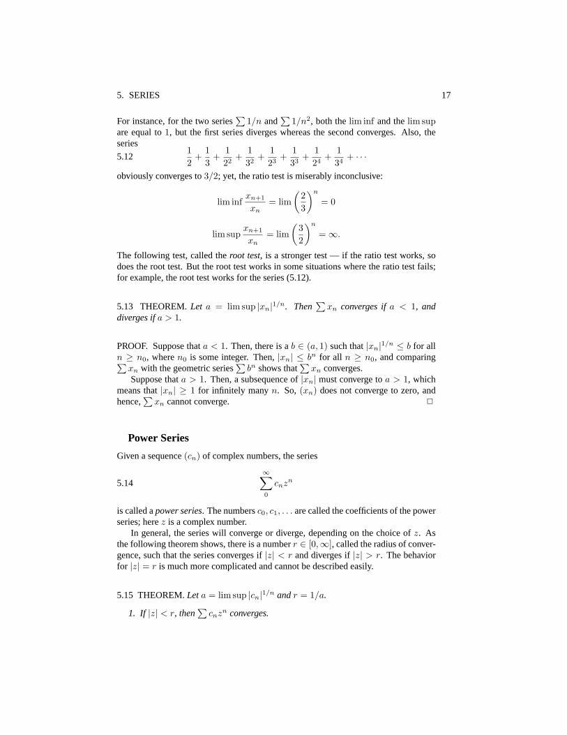
For instance, for the two series∑
1/n and∑
1/n2, both thelim inf and thelim supare equal to1, but the first series diverges whereas the second converges. Also, theseries
12
+13
+122
+132
+123
+133
+124
+134
+ · · ·5.12
obviously converges to3/2; yet, the ratio test is miserably inconclusive:
lim infxn+1
xn= lim
(23
)n
= 0
lim supxn+1
xn= lim
(32
)n
= ∞.
The following test, called theroot test, is a stronger test — if the ratio test works, sodoes the root test. But the root test works in some situations where the ratio test fails;for example, the root test works for the series (5.12).
5.13 THEOREM.Let a = lim sup |xn|1/n. Then∑
xn converges ifa < 1, anddiverges ifa > 1.
PROOF. Suppose thata < 1. Then, there is ab ∈ (a, 1) such that|xn|1/n ≤ b for alln ≥ n0, wheren0 is some integer. Then,|xn| ≤ bn for all n ≥ n0, and comparing∑
xn with the geometric series∑
bn shows that∑
xn converges.Suppose thata > 1. Then, a subsequence of|xn| must converge toa > 1, which
means that|xn| ≥ 1 for infinitely manyn. So, (xn) does not converge to zero, andhence,
∑xn cannot converge. 2
Power Series
Given a sequence(cn) of complex numbers, the series
∞∑0
cnzn5.14
is called apower series. The numbersc0, c1, . . . are called the coefficients of the powerseries; herez is a complex number.
In general, the series will converge or diverge, depending on the choice ofz. Asthe following theorem shows, there is a numberr ∈ [0,∞], called the radius of conver-gence, such that the series converges if|z| < r and diverges if|z| > r. The behaviorfor |z| = r is much more complicated and cannot be described easily.
5.15 THEOREM.Leta = lim sup |cn|1/n andr = 1/a.
1. If |z| < r, then∑
cnzn converges.

18 SETS AND FUNCTIONS
2. If |z| > r, then∑
cnzn diverges.
PROOF. Putxn = cnzn and apply the root test with
lim sup |xn|1/n = |z| lim sup |cn|1/n = a|z| = |z|r
.
2
5.16 EXAMPLE.
1.∑
zn/n! = ez andr = ∞.
2.∑
zn converges for|z| < 1 and diverges for|z| ≥ 1; r = 1.
3.∑
zn/n2 converges for|z| ≤ 1 and diverges for|z| > 1; r = 1.
4.∑
zn/n converges for|z| < 1 and diverges for|z| > 1; r = 1; for z = 1 theseries diverges, but for|z| = 1 butz 6= 1 it converges.
Absolute Convergence
The series∑
xn is said toconverge absolutelyif∑|xn| is convergent. If thexn are
all positive numbers, then absolute convergence is the same as convergence. UsingCauchy’s criterion (see Theorem 5.4) on both sides of
|m∑
i=n
xi| ≤m∑
i=n
|xi|
shows that if∑
xn converges absolutely then it converges. But the converse is not true:for example, ∑
(−1)n/n
converges but is not absolutely convergent.The comparison tests above, as well as the root and ratio tests, are in fact tests for
absolute convergence. If a series is not absolutely convergent, one has to study thesequence of partial sums to determine whether the series converges at all.

5. SERIES 19
Rearrangements
Let (k1, k2, . . .) be a sequence in which every integern ≥ 1 appears once and onlyonce, that is,n 7→ kn is a bijection fromN ontoN. If
yn = xkn, n ∈ N,
for such a sequence(kn), then we say that(yn) is a rearrangement of(xn).Let (yn) be a rearrangement of(xn). In general, the series
∑yn and
∑xn are
quite different. However, if∑
xn is absolutely convergent, then so is∑
yn and itconverges to the same number as does
∑xn. The converse is also true: if every rear-
rangement of the series∑
xn converges, then the series∑
xn is absolutely convergentand all its rearrangements converge (to the same sum).
On the other hand, if∑
xn is not absolutely convergent, its various rearrangementsmay converge or diverge, and in the case of convergence, the sum generally dependson the rearrangement chosen. For instance,
1− 12
+13− 1
4+
15− 1
6+
17− · · ·
is convergent, but not absolutely so. Its rearrangement
1 +13− 1
2+
15
+17− 1
4+
19
+ · · ·
(with + + − + + − + + − pattern) is again convergent, but not to the same sum. Infact, the following theorem due to Riemann shows that one can create rearrangementsthat are as bizarre as one wants.
5.17 THEOREM.Let∑
xn be convergent but not absolutely. Then, for any twonumbersa ≤ b in R there is a rearrangement
∑yn of
∑xn such that
lim infn∑1
yi = a, lim supn∑1
yi = b.
We omit the proof. Note that, in particular, takinga = b we can find a rearrangement∑yn with suma, no matter whata is.
Exercises:5.1 Determine the convergence or divergence of the following:
1.∑
(√
n + 1−√
n)
2.∑
(√
n + 1−√
n)/n
3.∑
(sinn)/(n√
n)
4.∑
(−1)nn/(n2 + 1).
In case of convergence, indicate whether it is absolute convergence.
20 SETS AND FUNCTIONS
5.2 Show that if∑
xn converges then so does∑√
xn/n .
5.3 Show that if∑
xn converges and(yn) is bounded and monotone (eitherincreasing or decreasing), then
∑xnyn converges.
5.4 Find the radius of convergence of each of the following power series:
1.∑
n2zn,
2.∑
2nzn/n!,
3.∑
2nzn/n2,
4.∑
n3zn/3n.
5.5 Suppose thatf(z) =∑
cnzn. Express the sum of the even terms,∑
c2nz2n,and the sum of the odd terms,
∑c2n+1z
2n+1, in terms off .
5.6 Suppose thatf(z) =∑
cnzn. Express∑
c3nz3n in terms off .
5.7 Rearrangements.Let∑
xn be a series that converges absolutely. Provethat every rearrangement of
∑xn converges, and that they all converge to
the same sum.
5.8 Riemann’s Theorem.Prove Riemann’s theorem 5.17 by filling in the de-tails in the following outline:
1. Let(x+n ) denote the subsequence consisting of the positive elements
of (xn) and let(x−n ) denote the subsequence of negative elements of(xn). Both of these sequences must be infinite.
2. Both sequences(x+n ) and(x−n ) converge to zero.
3. Both series∑
x+n and
∑x−n diverge.
4. Suppose thata, b ∈ R and define a rearrangement as follows: startwith the positive elements and choose elements from this set untilthe partial sum exceedsb. Then, choose elements from the set ofnegative elements until the partial sum is less thana. Then, chooseelements from the set of positive elements until the partial sum ex-ceedsb. Continue this proceedure of alternating between elementsof the positive and negative sets indefinitely.
5. Prove that the procedure described above can be continued ad infini-tum.
6. Prove that this rearrangement has the properties stated in Riemann’stheorem.
7. Extend the above arguments to the case wherea, b = ±∞.
5.9 Poisson distribution.Let pn = e−λλn/n! whereλ is a positive real. Showthat
1. pn > 0,

5. SERIES 21
2.∑∞
n=0 pn = 1,
3.∑∞
n=0 npn = λ.
5.10 Borel Summability.Consider a series∑∞
n=0 xn with partial sumssn =∑ni=0 xi. We say that the series isBorel summableif
limλ→∞
∞∑n=0
snpn
converges, wherepn are the Poisson probabilities defined in Exercise 5.9.For what values ofz is the geometric series
∑∞n=0 zn Borel summable?

22 SETS AND FUNCTIONS

Metric Spaces
Basic questions of analysis on the real line are tied to the notions of closeness anddistances between points. The same issue of closeness comes up in more complicatedsettings, for instance, like when we try to approximate a function by a simpler function.Our aim is to introduce the idea of distance in general, so that we can talk of the distancebetween two functions with the same conceptual ease as when we talk of the distancebetween two points in the plane. After that, we discuss the main issues: convergence,continuity, approximations. All along, there will be examples of different spaces anddifferent ways of measuring distances.
6 Euclidean Spaces
This section is to review the spaceRn together with its Euclidean distance. Recall thateach element ofRn is ann-tuplex = (x1, . . . , xn), where thexi are real numbers. Theelements ofRn are calledpointsor vectors, and we are familiar with the operations likeaddition of vectors and multiplication by scalars.
Inner Product and Norm
Forx andy in Rn, their inner productx · y is the number
x · y =n∑1
xiyi.6.1
If we regardx andy as column vectors, thenx · y = xT y. Forx in Rn, thenormof xis defined to be the positive number
‖x‖ =√
x · x =√∑n
1 x2i .6.2
The norm satisfies the following:
‖x‖ ≥ 0 for everyx in Rn,6.3
‖x‖ = 0 if and only if x = 0,6.4
‖x + y‖ ≤ ‖x‖+ ‖y‖ for all x andy in Rn.6.5
23

24 METRIC SPACES
Of these, 6.3 and 6.4 are obvious, and 6.5 is immediate from the following, which iscalled theSchwartz inequality.
6.6 PROPOSITION.|x · y| ≤ ‖x‖‖y‖ for all x andy in Rn.
PROOF. Consider the function
f(λ) = ‖λy − x‖2
= λ2‖y‖2 − 2λ(x · y) + ‖x‖2.
This function is clearly positive and quadratic and its minimum occurs at
λ =x · y‖y‖2
.
For this value ofλ we have
0 ≤ f(x · y‖y‖2
) = − (x · y)2
‖y‖2+ ‖x‖2
from which Schwartz’s inequality follows immediately. 2
Euclidean Distance
Forx andy in Rn, theEuclidean distancebetweenx andy is defined to be the number‖x− y‖. It follows from the properties given above that, for allx, y, z in Rn,
1. ‖x− y‖ ≥ 0,
2. ‖x− y‖ = ‖y − x‖,
3. ‖x− y‖ = 0 if and only if x = y,
4. ‖x− y‖+ ‖y − z‖ ≥ ‖x− z‖ .
The last is called thetriangle inequality: on R2, if the pointsx, y, z are the vertices ofa triangle, this is simply the well-known fact that the sum of the lengths of two sides isgreater than or equal to the length of the third side.
The setRn together with the Euclidean distance is calledn-dimensional Euclideanspace. The Euclidean spaces are important examples of metric spaces.
Exercises:6.1 Show that the mapping(x, y) 7→ x · y from Rn × Rn into R is a linear
transformation inx and is a linear transformation iny (and therefore issaid to be bilinear). Conclude that
(x + y) · (x + y) = x · x + 2x · y + y · y.
Use this and the Schwartz inequality to prove (6.5).
7. METRIC SPACES 25
6.2 Show that‖x + y‖2 + ‖x − y‖2 = 2‖x‖2 + 2‖y‖2. Interpret this ingeometric terms, onR2, as a statement about parallelograms.
6.3 Pointsx andy are said to beorthogonal if x · y = 0. Show that thisis equivalent to saying that the lines connecting the origin tox andy areperpendicular. In general, lettingα be the angle between the lines throughx andy, we havex · y = ‖x‖‖y‖ cos α.
7 Metric Spaces
Let E be a set. AmetriconE is a functiond : E×E 7→ R+ that satisfies the followingfor all x, y, z in E:
1. d(x, y) = d(y, x),
2. d(x, y) = 0 if and only if x = y,
3. d(x, y) + d(y, z) ≥ d(x, z).
A metric spaceis a pair(E, d) whereE is a set andd is a metric onE. In this context,we think of E as a space, call the elements ofE points, and refer tod(x, y) as thedistance fromx to y.
EXAMPLES.
7.1 Euclidean spaces.ConsiderRn with the Euclidean distanced(x, y) = ‖x − y‖on it. It follows from (1)–(4) thatd is a metric onRn. Thus,(Rn, d) is a metric spaceand is calledn-dimensional Euclidean space.
7.2 Manhattan metric.OnRn define a metricd by
d(x, y) =n∑1
|xi − yi|.
This d is called the Manhattan metric, orl1-metric, onRn, and(Rn, d) is a metricspace again. Note that forn > 1 this metric is different from the Euclidean metric ofthe preceding example.
7.3 SpaceC. Let C denote the set of all continuous functions from the interval[0, 1]into R. Forx andy in C, let
d(x, y) = sup0≤t≤1
|x(t)− y(t)|.

26 METRIC SPACES
It is clear thatd(x, y) is a positive real number, thatd(x, y) = d(y, x), and thatd(x, y) = 0 if and only if x = y. As for the triangle inequality, we note that
|x(t)− z(t)| ≤ |x(t)− y(t)|+ |y(t)− z(t)| ≤ d(x, y) + d(y, z)
for every t in [0, 1], from which we haved(x, y) + d(y, z) ≥ d(x, z). Thus,d is ametric onC, and(C, d) is a metric space. This metric space is important in analysis.
Usage
In the literature, it is common practice to callE a metric space if(E, d) is a metricspace for some metricd. If there is only one metric under consideration, this is harmlessand saves time. For instance, the phrase “Euclidean spaceRn” refers to(Rn, d) whered is the Euclidean metric. For a while at least, we shall indicate the metric involved ineach case in order to avoid all possible confusion.
Distances from Points to Sets and from Sets to Sets
Let (E, d) be a metric space. Forx in E andA ⊂ E, let
d(x, A) = inf{d(x, y) : y ∈ A};7.4
this is called the distance from the pointx to the setA. For A ⊂ E andB ⊂ E, thedistance fromA to B is defined by
d(A,B) = inf{d(x, y) : x ∈ A, y ∈ B}.7.5
Thediameterof a setA ⊂ E is defined to be
diamA = sup{d(x, y) : x ∈ A, y ∈ A}.7.6
A set is said to beboundedif its diameter is finite.
Balls
Let (E, d) be a metric space. Forx in E andr in (0,∞),
B(x, r) = {y ∈ E : d(x, y) < r}7.7
is called theopen ballwith centerx andradiusr, and
B(x, r) = {y ∈ E : d(x, y) ≤ r}7.8
is the correspondingclosed ball.For example, ifE = R3 andd is the usual Euclidean metric, thenB(x, r) becomes
the set of all points inside the sphere with centerx and radiusr, andB(x, r) is the setof all points inside or on that sphere.
Exercises and Complements:
7. METRIC SPACES 27
7.1 Discrete metric.Let E be an arbitrary set. Define
d(x, y) =[
1 if x 6= y,0 if x = y.
Show that thisd is a metric onE. It is called the discrete metric onE.
7.2 Metrics onRn. For each numberp ≥ 1,
dp(x, y) = (n∑1
|xi − yi|p)1/p
defines a metricdp onRn. Note thatd1 is the Manhatten metric, andd2 isthe Euclidean metric. Finally,
d∞(x, y) = sup1≤i≤n
|xi − yi|
is again a metric onRn. Show this.
7.3 Equivalent Metrics. Two metricsd and d′ are equivalent if there existstrictly positive constantsc1 andc2 such that for allx, y:
c1d′(x, y) ≤ d(x, y) ≤ c2d
′(x, y).
Show thatd1, d2, andd∞ are all equivalent to each other.
7.4 Weighted Metrics onRn. The metrics introduced in the preceding exercisetreat all components ofx−y equally. This is reasonable ifRn is thought ofgeometrically and the selection of a coordinate system is unimportant. Onthe other hand, ifx = (x1, . . . , xn) stands for a shopping list that requiresbuying x1 units of product one, andx2 units of product two, and so on,then it would make much better sense to define the distance between twoshopping listsx andy by
d(x, y) =n∑1
wi|xi − yi|
wherex1, . . . , wn are fixed, strictly positive numbers, withwi being thevalue of one unit of producti. Show that thisd is indeed a metric. Moregenerally, paralleling the metrics introduced in the previous exercise,
dp(x, y) = (n∑i
wi|xi − yi|p)1/p, x, y ∈ Rn,
is a metric onRn for eachp ≥ 1 and each fixed, strictly positive vectorw(the latter meansw1 > 0, . . . , wn > 0).

28 METRIC SPACES
7.5 l2-Spaces.Instead ofRn, now consider the spaceR∞ of all infinite se-quences inR, that is, eachx in R∞ is a sequencex = (x1, x2, . . .) of realnumbers. In analogy with thed2 metrics introduced onRn in Exercises7.2 and 7.4, we define
d2(x, y) = (∞∑1
|xi − yi|2)1/2.
Thisd2 satisfies all the conditions for a metric except thatd2(x, y) can be∞ for somex andy. To remedy the latter, we letE be the set of allx inR∞ with
∞∑1
x2i < ∞.
Then, by an easy generalization of the Schwartz inequality, it follows thatd2(x, y) < ∞ for all x andy in E. Thus,(E, d2) is a metric space. It isgenerally denoted byl2.
7.6 Metrics onC. Consider the setC of all continuous functions from[0, 1]into R. The interval[0, 1] can be replaced by any bounded interval[a, b],in which case one writesC([a, b]). A number of metrics can be definedon C in analogy with those in Exercise 7.2. The analogy is provided bythe following observation: everyx in Rn can be thought of as a functionx from { 1
n , 2n , . . . , n
n} into R, namely, the functionx with x(t) = xi fort = i/n. Thus, replacing the set{ 1
n2n , . . . , n
n} with the interval[0, 1] andreplacing the summation by integration, we obtain
dp(x, y) = (∫ 1
0
|x(t)− y(t)|pdt)1/p
for all x andy in C. Since any continuous function on[0, 1] is bounded,the integral here is finite and it is easy to check the conditions for thisdp tobe a metric, except perhaps for the triangle inequality. So, for eachp ≥ 1,this dp is a metric onC. Incidentally, the metric of Example 7.3 can bedenoted byd∞ in analogy withd∞ in Exercise 7.2.
7.7 Open Balls.Let E = R2. Describe the open ballB(x, r), for fixedx andr, under each of the following metrics:
1. d2 of Exercise 7.2.
2. d1 of Exercise 7.2.
3. d∞ of Exercise 7.2.
4. d2 of Exercise 7.4 withw1 = 1 andw2 = 5.
7.8 Open Balls inC. For the metric space of Example 7.3, describeB(x, r)for a fixed functionx and fixed numberr > 0. Draw pictures!

8. OPEN AND CLOSED SETS 29
7.9 Product Spaces.Let (E1, d1) and(E2, d2) be arbitrary metric spaces. LetE = E1 × E2 and define, forx = (x1, x2) in E andy = (y1, y2) in E,
d(x, y) = [d1(x1, y1)2 + d2(x2, y2)2]1/2.
Show thatd is a metric onE. The metric space(E, d) is called the productof the metric spaces(E1, d1) and(E2, d2).
8 Open and Closed Sets
Let (E, d) be a metric space. All points mentioned below are points ofE, all sets aresubsets ofE. Recall the definition 7.7 of the open ballB(x, r) with centerx and radiusr.
8.1 DEFINITION. A setA is said to beopenif for everyx in A there is anr > 0 suchthatB(x, r) ⊂ A. A set is said to beclosedif its complement is open.
For example, ifE = R with the usual distance, the intervals(a, b), (−∞, b), (a,∞)are open, the intervals[a, b], (−∞, b], [a,∞) are closed, and the interval(a, b] is neitheropen nor closed.
8.2 PROPOSITION.Every open ball is open.
PROOF. Fixx andr. To show thatB(x, r) is open, we need to show that for everyy inB(x, r) there is aq > 0 such thatB(y, q) ⊂ B(x, r). This is accomplished by pickingq = r − d(x, y). Sincey is in B(x, r), we haved(x, y) < r and, hence,q > 0. And,every point ofB(y, q) is a point ofB(x, r), becausez ∈ B(y, q) meansd(z, y) < qwhich implies that
d(z, x) ≤ d(z, y) + d(y, x) < q + d(y, x) = r.
2
8.3 THEOREM.The sets∅ and E are open. The intersection of a finite number ofopen sets is open. The union of an arbitrary collection of open sets is open.
PROOF. The first assertion is trivial from the definition.We prove the second assertion for the intersection of two open sets. The general
case follows from the repeated aplication of the case for two. LetA andB be open.Let x ∈ A ∩ B. SinceA is open andx is in A, there isp > 0 such thatB(x, p) ⊂ A.

30 METRIC SPACES
Similarly, there is aq > 0 such thatB(x, q) ⊂ B. Let r = p∧q, the smaller ofp andq.Then,B(x, r) ⊂ B(x, p) ⊂ A andB(x, r) ⊂ B(x, q) ⊂ B. Hence,B(x, r) ⊂ A∩B.So,A ∩B is open.
For the last assertion, let{Ai : i ∈ I} be an arbitrary collection of open sets. Wewant to show thatA = ∪iAi is open. Letx be inA. Then,x ∈ Ai for somei ∈ I.SinceAi is open, there is anr > 0 such thatB(x, r) ⊂ A. SinceAi ⊂ A, this showsthatB(x, r) ⊂ A. So,A is open. 2
The following characterization is immediate from the preceding theorem togetherwith Proposition 8.2.
8.4 PROPOSITION.A set is open if and only if it is the union of a collection of openballs.
PROOF. IfA is the union of a collection of open balls, thenA must be open in viewof 8.2 and 8.3. To show the converse, letA be open. Then, for everyx in A, there isan open ballAx = B(x, r(x)) contained inA. Obviously, the union of all theseAx isexactlyA. 2
Closed Sets
Recall that a subset ofE is closed if and only if its complement is open. Thus, the fol-lowing theorem is immediate from Theorem 8.3 above and the fact that the complementof a union is the intersection of complements and vice versa.
8.5 THEOREM.The sets∅ andE are closed. The union of finitely many closed sets isclosed. The intersection of an arbitrary collection of closed sets is closed.
Every closed ball is closed. This last observation can be proved along the lines of8.2: if y ∈ E \ B(x, r) thend(y, x) > r, and pickingp = d(x, y)− r > 0 we see thatB(y, p) ⊂ E \ B(x, r), which proves thatE \ B(x, r) is open. In particular, for eachx in E, the singleton{x} is closed. It follows from this and the preceding theorem thatevery finite set is closed.
Interior, Closure, and Boundary
Let A be a subset ofE. The collection of all closed sets containingA is not empty(sinceE belongs to that collection.) The intersectionA of that collection is a closedset by the last theorem. Clearly,A is the smallest closed set that containsA, that is, ifB ⊃ A andB is closed thenB ⊃ A. The setA is called theclosureof A.
We define theinterior of A similarly as the largest open set contained inA, and wedenote it byA◦. In other words,A◦ is the union of all open sets contained inA. Note

8. OPEN AND CLOSED SETS 31
thatA◦ ⊂ A ⊂ A.8.6
We define theboundaryof A to be the set∂A = A \A◦.For example, ifA is the open ballB(x, r) in the Euclidean spaceE = Rn, the
A◦ = A, A = B(x, r), and∂A is the sphere of radiusr centered atx. If E = R withthe usual metric, and ifA = (a, b], thenA = [a, b] andA◦ = (a, b) and∂A = {a, b}.The following seems self evident.
8.7 PROPOSITION.A set is closed if and only if it is equal to its closure. A set is openif and only if it is equal to its interior.
Open Subsets of the Real Line
We takeE = R with the usual distance. Then, every open ball is an open interval, andaccording to Proposition 8.4, every open set is the union of a collection of open balls.The following sharpens the picture by taking into account the special nature of the realline.
8.8 THEOREM.A subset ofR is open if and only if it is the union of a countablecollection of disjoint open intervals.
PROOF. The “if” part is immediate from Proposition 8.4 and the fact that every openball is an interval in this case.
To prove the “only if” part, letA be an open subset ofR. Recall that the setQ ofall rationals is countable. For eachq in Q ∩A, let
aq = sup{y ≤ q : y 6∈ A}, bq = inf{y ≥ q : y 6∈ A}.
Then,B =
⋃q∈Q∩A
(aq, bq)
is the union of a countable collection of open intervals. We show next thatA = B byshowing thatA ⊂ B andB ⊂ A.
Let x be in A. SinceA is open, there is a ballB(x, r) contained inA. Take arational numberq in this ball. Clearly,B(x, r) ⊂ (aq, bq). Thus,x is in B. Since thisis true for everyx in A, we have thatA ⊂ B.
Fix q ∈ Q ∩A. Clearly,(aq, bq) ⊂ A. Hence,B ⊂ A.We have shown thatA = B, andB has the desired form except that the intervals
(aq, bq) are not necessarily disjoint. Note that ifr ∈ (aq, bq) then(ar, br) = (aq, bq)andq ∈ (ar, br). Let us writeq ≈ r if and only if (aq, bq) = (ar, br). This definesan equivalence relation on the setQ ∩ A. Thus, by picking exactly oneq from each

32 METRIC SPACES
0 1
Figure 2: The setD = ∪Dq.
equivalence class, we can form a setI ⊂ Q ∩ A such that(aq, bq) ∩ (ar, br) = ∅ forall distinctq andr in I, and
A = B =⋃q∈I
(aq, bq).
2
8.9 EXAMPLE.The Cantor Set.Start with the unit intervalB = [0, 1]. To eachq in the setI =
{1/2; 1/4, 3/4; 1/8, 3/8, 5/8, 7/8; 1/16, 3/16, . . . , 15/16; . . .} we associate anopen intervalDq in the following fashion:D1/2 is the open interval(1/3, 2/3) whichis the middle third ofB. Deleting it fromB leaves two closed intervals,[0, 1/3] and[1/3, 1]. Let D1/4 be the interval(1/9, 2/9), which is the middle third of[0, 1/3],and letD3/4 be (7/9, 8/9), which is the middle third of[2/3, 1]. Deleting thosemiddle thirds, we are left with four closed intervals of length1/9 each. LetD1/8,D3/8, D5/8, D7/8 be the open intervals that make up the middle thirds of those closedintervals. Delete the middle thirds, and continue in this manner (see Figure 2). Then,
D =⋃q∈I
Dq
is the union of the countably many disjoint open intervalsDq, q ∈ I. It is an exampleof a non-trivial open set. Incidentally, note that the lengths of theDq sum to
13
+ (19
+19) + (
127
+127
+127
+127
) + · · · = 1.
Thus, the “length” ofD is 1. But the setC = B \D is not empty.The setC = B \ D is called theCantor set. It is obviously a closed set. The
construction above shows thatC is obtained by starting withB and deleting the middlethird of every interval we can find. Thus, there is no open interval contained inC. Thatis, there are no open balls inC. Hence, the interior ofC must be empty, andC is pureboundary:
C◦ = ∅, C = C, ∂C = C.
Also, since the length ofD is equal to the length ofB, the length ofC = B \D mustbe0. In summary, the Cantor set is very thin.

8. OPEN AND CLOSED SETS 33
x=g(y)
y=f(x)
Figure 3: The cantor function.
Nevertheless,C has at least as many points as the interval[0, 1]. We prove this nextby showing, via construction, that there exists an injectiong from [0, 1] into C.
To this end, we start by defining an increasing functionf from D into [0, 1] byletting
f(x) = q, if x ∈ Dq.
Then, we define the functiong on [0, 1] by settingg(1) = 1 and
g(y) = inf{x ∈ D : f(x) > y}, 0 ≤ y < 1.
We show first thatg(y) ∈ C for everyy. This is obvious fory = 1. Let y ∈ [0, 1);note thatg(y) is the infimum of the union of all intervalsDq with q > y; clearly,that infimum cannot belong toD; so g(y) must belong toC (since it is obvious thatg(y) ∈ B). Finally, we show thatg : [0, 1] 7→ C is an injection by showing that ify < z, theng(y) < g(z). Fix y < z. Note that there is at least oneq in I such thaty < q < z, and the corresponding setDq is contained in{x ∈ D : f(x) > y} but notin {x ∈ D : f(x) > z}. It follows that the numberg(y) is to the left of the intervalDq
whereasg(z) is to the right. So,g(y) < g(z) if y < z. Hence,g : [0, 1] 7→ C is aninjection.
Exercises and Complements:8.1 Let(E, d) be a metric space. Show that
A = {x ∈ E : d(x,A) = 0}A◦ = {x ∈ E : d(x,Ac) > 0}∂A = {x ∈ E : d(x,A) = 0 andd(x,Ac) = 0}.
34 METRIC SPACES
8.2 Let (E, d) be a metric space. FixA ⊂ E. Show thatAε = {x ∈ E :d(x,A) < ε} is an open set containingA for eachε > 0. Show thatA = ∩ε>0Aε.
8.3 Boundedness.Let (E, d) be a metric space. Show that a subsetA of E isbounded if and only if it is contained in some ball, that is, if and only ifA ⊂ B(x, r) for somex andr.
8.4 TakeE = R andd the usual metric. LetA ⊂ E. Show that ifA is closedand bounded above, thensupA belongs toA (that is,A has a maximum).Similarly, if A is closed and bounded below, then it has a minimum. Showthat an open setA cannot have a minimum, that is,inf A cannot belong toA.
8.5 LetD be the open set of Example 8.9. Find its interior and boundary.
8.6 Denseness.A setD is said to bedensein E if D = E. Let D be dense inE. Show that everyx in E is at0 distance fromD. Thus, every open ballhas at least one point ofD. Show that the setQ of all rationals is dense inR, the set of all pairs of rationals is dense inR2, etc.
8.7 Separability.The metric spaceE is said to be separable if there exists acountable setD that is dense inE. So, for example, the Euclidean spacesR, R2, R3, ... are separable.
8.8 Discrete metric spaces.Let E be arbitrary and suppose thatd is the dis-crete metric (see (7.1) for it) onE. Show that each subsetA is both openand closed. Forr ≤ 1, every open ballB(x, r) consists of exactly thepoint x. Note thatB(x, 1) = {x}, B(x, 1) = E for every x (Moral:B(x, r) is not necessarily the closure ofB(x, r)). If E is countable, thenit is separable (trivially). IfE is uncountable, it is not separable. Showthis.
9 Convergence
Let (E, d) be a metric space. Our goal is to discuss the notion of convergence for asequence of points inE. We do so by employing the concept of convergence inR, forwhich we refer to Section 4 of Chapter .
9.1 DEFINITION. A sequence(xn) in E is said to beconvergentin E if there existsa pointx in E such thatlim d(xn, x) = 0. And, then,(xn) is said toconvergeto x, thepointx is called thelimit of (xn), and the notationx = lim xn is used to indicate it.
REMARK: The preceding definition includes, implicit in it, the fact that a convergent

9. CONVERGENCE 35
sequence has exactly one limit. To see this, suppose that(xn) converges tox and toy,that is,lim d(xn, x) = 0 andlim d(xn, y) = 0. Then,
0 ≤ d(x, y) ≤ d(x, xn) + d(xn, y)
by the triangle inequality, and the right side converges to zero. Thus,d(x, y) = 0,which means thatx = y.
The following brings together a number of re-wordings of convergence. Each is aslight alteration of the others. No proof seems needed.
9.2 THEOREM.The following statements are equivalent:
1. (xn) converges tox.
2. For everyε > 0 there is annε such thatd(xn, x) < ε for all n ≥ nε.
3. The set{n : d(xn, x) ≥ ε} is finite for eachε > 0.
4. For everyε > 0, the ballB(x, ε) includes all but a finite number of the termsxn.
9.3 COROLLARY.Every convergent sequence is bounded.
PROOF. Let(xn) be convergent andx its limit. In view of the equivalence of 1 and 4in Theorem 9.2,B(x, 1) includes all but a finite number of the termsxn. Let r be themaximum of the distances fromx to those termsxn outsideB(x, 1), if there are any;otherwise, setr = 1. Clearlyr < ∞ andB(x, r) contains(xn), which means that(xn) is bounded. 2
Subsequences
It follows from Theorem 9.2 that we may remove a finite number of terms, or rearrangethe terms, without affecting the convergence. The following generalizes this.
9.4 PROPOSITION.If a sequence converges tox, then every subsequence of it con-verges to the samex.
PROOF. Let(xn) be a sequence with limitx. Let (yn) be a subsequence of it, thatis, yn = xkn
for somek1 < k2 < · · ·. Now, by Theorem 9.2, for everyε > 0 theball B(x, ε) includes all the termsxn except for some finite number of them; thereforethe same must be true for the termsyn. So, by Theorem 9.2, the subsequence(yn)converges tox. 2

36 METRIC SPACES
Convergence and Closed Sets
Think of a particle that moves inE by jumps: first it is atx1, then atx2, then atx3, andso on. The following gives meaning to the term “closed set” if you think of sequencesin this fashion.
9.5 THEOREM.A set is closed if and only if it includes the limit of every sequence init.
PROOF. “Only if” part. Suppose thatA is a closed set and that(xn) is a sequence inA with limit x. We show that, then,x must belong toA. For, otherwise, ifx were inAc, there would exist anε > 0 such thatB(x, ε) ⊂ Ac sinceAc is open andB(x, ε)would include infinitely many terms sincex is the limit, which would contradict thefact that all thexn are inA.
“If” part. We show that ifA is not closed then there is a sequence(xn) in A thatconverges to some pointx in Ac. Suppose thatA is not closed. ThenAc is not open.Thus, there exists anx in Ac such thatB(x, r)∩A has at least one point for eachr > 0.Hence, for eachn in N, there is anxn in A such thatd(xn, x) < 1/n. Obviously,(xn)is in A and converges tox which is not inA. 2
Exercises:
9.1 Discrete metric spaces.Suppose thatd is the discrete metric onE. Showthat (xn) is convergent if and only if it is ultimatelystationary, that is, ifand only if it has the form(x1, x2, . . . , xn, x, x, x, . . .) for somen.
9.2 Let (E, d) be arbitrary. Show that if(xn) converges tox and(yn) con-verges toy, thend(xn, yn) converges tod(x, y). Hint: first show that, forarbitraryx, y, z in E,
|d(x, y)− d(x, z)| ≤ d(y, z).
Use this to write
|d(xn, yn)− d(x, y)| ≤ |d(xn, yn)− d(xn, y)|+|d(xn, y)− d(x, y)|
≤ d(yn, y) + d(xn, x),
and take limits.
9.3 Show that if(xn) converges tox, thend(xn, A) converges tod(x,A) foreach fixed subsetA of E.
10. COMPLETENESS 37
10 Completeness
Let (E, d) be a metric space. Recall that a sequence(xn) in E is convergent if thereis anx in E such thatlim d(xn, x) = 0. This definition has two shortcomings. First,starting with(xn), we rarely have a candidatex for the limit. Second, often we arenot interested in computing the limit itself; it is generally sufficient to know that thelimit exists and has such and such properties. This section is aimed at rectifying theseshortcomings.
Cauchy Sequences
10.1 DEFINITION. A sequence(xn) in E is said to beCauchyif for everyε > 0 thereis annε such thatd(xm, xn) < ε for all m > n ≥ nε.
The following is nearly a re-statement of this definition in slightly more geometricterms.
10.2 LEMMA. A sequence(xn) is Cauchy if and only if for everyε > 0 there is a ballof radiusε that contains all but finitely many of the termsxn.
PROOF. Suppose that(xn) is Cauchy. Letε > 0. Then, there isnε such thatd(xm, xn) < ε for all m > n ≥ nε. Thus, in particular, the ballB(xnε
, ε) contains allthe terms except possiblyx1, . . . , xnε−1. This proves the necessity of the condition.
Conversely, suppose that for everyε > 0 there is a ballB(x, ε) with somex as itscenter such that all but a finite number of the terms are in the ball. Givenε > 0, nowpick x so thatB(x, ε/2) contains all thexn except perhaps finitely many, that is, thereis nε such thatxn ∈ B(x, ε/2) for all n ≥ nε. Now, if m > n ≥ nε, then
d(xm, xn) ≤ d(xm, x) + d(x, xn) < ε/2 + ε/2 = ε.
Hence,(xn) is Cauchy. This proves the sufficiency. 2
10.3 THEOREM.
1. Every convergent sequence is Cauchy.
2. Every Cauchy sequence is bounded.
3. Every subsequence of a Cauchy sequence is Cauchy.

38 METRIC SPACES
PROOF. The first claim is immediate from the preceding lemma and Theorem 9.2. Thesecond claim is proved, via the preceding lemma, by following the proof of Corollary9.3. The last claim is immediate from the preceding lemma. 2
The following shows that if a sequence is Cauchy and you can find a subsequenceof it that converges to some pointx, then the original sequence converges tox.
10.4 PROPOSITION.A Cauchy sequence that has a convergent subsequence is itselfconvergent.
PROOF. Let(xn) be Cauchy. Letx be the limit of a convergent subsequence of it.Pickε > 0. By Lemma 10.2, there is a ballB(y, ε) that contains all but a finite numberof thexn. That ballB(y, ε) must contain all but a finite number of the subsequence aswell. Thus,x must be inB(y, ε). Then,B(x, 3ε) containsB(y, ε) and hence containsall but a finite number of thexn. Thus,(xn) is convergent andx = lim xn in view ofTheorem 9.2. 2
Complete Metric Spaces
All the results above suggest that all Cauchy sequences should be convergent, which isin fact what we hope for. Unfortunately, this is not true in general. Here is an example.
Suppose thatE = Q, the set of all rationals, with the metric it inherits from thereal line. Letx =
√2, which is not a rational number, and let(xn) be a sequnce in
Q that converges tox in the sense of convergence inR: for instance, pickxn to be arational number in the interval(x, x + 1/n) for eachn. Over the metric spaceQ, thesequence(xn) is Cauchy, but fails to be convergent inQ simply becausex is not inQ.The problem here is not with the Cauchy sequence, but with the spaceQ. The spaceQhas holes in it!
The following introduces the extra notion we want.
10.5 DEFINITION. The metric space(E, d) is said to becompleteif every Cauchysequence inE converges to a point ofE.
The following is immediate from Theorem 9.5.
10.6 PROPOSITION.If (E, d) is complete andD ⊂ E is closed, then(D, d) is acomplete metric space.
The following shows that familiar spaces are complete. Other examples are listedin exercises.

10. COMPLETENESS 39
10.7 THEOREM.Every Euclidean space is complete.
PROOF. We start with the one-dimensional Euclidean space, namelyR. Let (xn) ⊂ Rbe Cauchy. Then, for everyε > 0 there is a ball of radiusε (namely an open intervalof length2ε) that contains all but finitely many of thexn. Therefore, the numbersx = lim inf xn andy = lim supxn must belong to that ball, which means that0 ≤y − x < 2ε. Since this is true for everyε > 0, we must havex = y, that is,(xn) isconvergent. This proves thatR is complete.
Now, fix k ≥ 2 and consider the Euclidean spaceRk. We writex = (a, b, . . . , c)for eachx in Rk for simplicity of notation (in other words, the coordinates ofx area, b, . . . , c).
Consider a Cauchy sequence of pointsxn = (an, bn, . . . , cn) in Rk. Givenε > 0,then, for allm andn large enough, we have
d(xm, xn) = (|am − an|2 + |bm − bn|2 + · · ·+ |cm − cn|2)1/2 < ε,
which shows that
|am − an| < ε, |bm − bn| < ε, . . . , |cm − cn| < ε.
In other words, the sequences(an), (bn), ...,(cn) in R are Cauchy. We have just shownthat R is complete. So, these sequences must be convergent inR, say, with limitsa, b, . . . , c respectively. Now, letx = (a, b, . . . , c) and note that
d(xn, x)2 = |an − a|2 + |bn − b|2 + · · ·+ |cn − c|2
converges to0. Hence,lim d(xn, x) = 0, and(xn) is convergent. This completes theproof thatRk is complete. 2
Exercises and Complements:10.1 Show that the following metric spaces are complete:
1. E = R2 with the Manhattan metricd.
2. E arbitrary,d is the discrete metric.
In fact, eachRk is a complete metric space with any one of the metricsdp
introduced in Exercises 7.2 and 7.4.
10.2 Show that the spacel2 introduced in Exercise 7.5 is complete. Incidently,so is the spaceC of Example 7.3 and Exercise 7.6.
10.3 Two Cauchy sequences(xn) and (yn) are said to be equivalent if theirmerger(x1, y1, x2, y2, . . .) is Cauchy. In this case, we write(xn) ≡ (yn).Show that this defines an requivalence relation. That is,
1. (xn) ≡ (xn)2. (xn) ≡ (yn) implies that(yn) ≡ (xn)3. (xn) ≡ (yn), (yn) ≡ (zn) implies that(xn) ≡ (zn).

40 METRIC SPACES
11 Compactness
Let (E, d) be a metric space. It will be convenient to refer toE as a metric space,without mentioningd. We shall use the picturesque phrase “the collection{Ai : i ∈ I}covers B” to mean that∪i∈IAi ⊃ B.
11.1 DEFINITION. A setC ⊂ E is said to becompactif every collection of open setsthat coversC has a finite sub-collection that coversC. The metric space(E, d) is saidto be compact ifE is so.
We shall show that, for many metric spaces, compact sets are precisely the sets thatare bounded and closed. The following are aimed in that direction. The proofs areexcessively detailed in order to facilitate understanding.
11.2 PROPOSITION.Every compact set is bounded.
PROOF. LetC be compact. For eachx in C, letBx be a ball of radius1 centered atx.Obviously, then, the collection{Bx : x ∈ C} of open sets coversC. Hence, there mustbe a finite sub-collection, say of setsBx1 , . . . , Bxn , that coversC. Since the union ofballsBx1 , . . . , Bxn must be bounded, this implies thatC is bounded as well. 2
11.3 PROPOSITION.Every closed subset of a compact set is compact.
PROOF. LetD be compact. LetC ⊂ D be closed. Fix a collection of open sets thatcoversC. Adding the open setE \ C to that collection, we obtain a collection of opensets that coversD. SinceD is compact, the latter collection has a finite sub-collectionthat still coversD. RemovingE \C from that sub-collection (if it were in), we obtain afinite sub-collection of the original collection that coversC. Thus,C must be compact.2
Compact Subspaces
Recall that every subsetD of E can be regarded as a metric space by itself, with themetric it inherits fromE. WhetherD is open or not as a subset ofE, it is openautomatically when it is regarded as a metric space. The concept of compactness doesnot suffer from such foolishness.
11.4 PROPOSITION.A setD is compact as a metric space if and only if it is compactas a subset ofE.

11. COMPACTNESS 41
PROOF. A subset ofD is an open ball in the spaceD if and only if it has the formB ∩D for some open ballB of the spaceE. Since an open set is the union of all theopen balls it contains, it follows thatA is an open subset of the spaceD if and only ifA = B∩D for some open subsetB of the spaceE. Now, the definition of compactnessdoes the rest. 2
Cluster Points, Convergence, Completeness
This is to look into the connections between compactness and convergence.
11.5 DEFINITION. A pointx in E is called acluster point2 of a subsetA of Eprovided that every open ball centered atx contains infinitely many points ofA.
11.6 THEOREM.Every infinite subset of a compact set has at least one cluster pointin that compact set.
PROOF. We shall show that ifC is compact, andA ⊂ C, andA has no cluster pointin C, thenA is finite. LetA andC be such. Since nox in C is a cluster point ofA, foreveryx in C there is an open ballB(x, r) that contains only finitely many points ofA.Those open balls coverC obviously. SinceC is compact, there must be a finte numberof them that coverC and, therefore,A. Since each one of those finitely many balls hasa finte number of points ofA, the total number of points inA must be finite. 2
The following is the way compactness helps in discussing convergence. In particu-lar, together with Proposition 10.4, it shows that every Cauchy sequence in a compactset is convergent.
11.7 THEOREM.Every sequence in a compact set has a subsequence that convergesto some point of that set.
PROOF. LetC be compact. Let(xn) ⊂ C. If the setA = {x1, x2, . . .} is finite,then at least one point ofA, sayx, appears infinitely often in the sequence, and hence(x, x, . . .) is a subsequence, which obviously converges tox ∈ A ⊂ C. Now supposethatA is infinite. By the preceding theorem, thenA has a cluster pointx in C. Sinceeach one of the ballsB(x, 1/n), n = 1, 2, . . ., has infinitely many points inC, wemay pickk1 so thatxk1 is in B(x, 1), pick k2 > k1 so thatxk2 is in B(x, 1/2), pickk3 > k2 so thatxk3 is in B(x, 1/3), and so on. Obviously,(xkn
) converges tox. 2
2Other terms in common use include limit point, adherence point, point of accumulation, etc.
42 METRIC SPACES
11.8 COROLLARY.Every compact set is closed.
PROOF. LetC be compact. The preceding theorem implies that every convergentsequence inC converges to a point ofC. Thus,C is closed by Theorem 9.5. 2
11.9 COROLLARY.Every compact metric space is complete. Every Cauchy sequencein a compact metric space is convergent.
PROOF. The second statement is immediate from Theorem 11.7 and Proposition 10.4.The first follows from the second by the definition of completeness. 2
Compactness in Euclidean Spaces
We have seen that, for an arbitrary metric space, every compact set is bounded andclosed (Proposition 11.2 and Corollary 11.8). In the case of Euclidean spaces, theconverse is true as well. This is called theHeine-Borel Theorem.
11.10 THEOREM.A subset of a Euclidean space is compact if and only if it is boundedand closed.
We start by listing an auxiliary result that is trivial at least forR, R2, R3. We omitits proof.
11.11 LEMMA. Let B be a bounded subset of a Euclidean spaceE. Then, for everyε > 0 there is a finite collection of closed balls of radiusε that coversB.
Here is the proof of Theorem 11.10.
PROOF. As mentioned above, 11.2 and 11.8 prove the necessity part. We now provethe sufficiency of the condition.
LetE be a Euclidean space and letC be a closed and bounded subset ofE. SupposethatC is not compact. Then, there is a collection{Ai : i ∈ I} of open sets that coversC but is such that
no finite sub-collection{Ai : i ∈ I} coversC.11.12
(a) Letε = 1/2. By the preceding lemma, we can find a finite numberm of closedballsB1, . . . , Bm of radiusε that coverC. Then,C = (C ∩B1)∪ · · · ∪ (C ∩Bm). Inview of (11.12), at least one ofC ∩B1, . . . , C ∩Bm cannot ever be covered by a finitesub-collection of theAi; let that one be denoted byC1. Now,C1 is closed, its diameteris at most2ε = 1 (since theBk have diameter1), and (11.12) is true forC1.

11. COMPACTNESS 43
(b) Applying the arguments of the preceding paragraph withε = 1/4 to the setC1 we get a new setC2 ⊂ C1 that is closed, has diameter at most1/2, and (11.12)holds forC2. Repeating this withε = 1/6, 1/8, 1/10, . . . we obtain further setsC3, C4, C5, . . . with the same properties but with diameters at most1/3, 1/4, 1/5, . . ..ClearlyC1 ⊃ C2 ⊃ C3 ⊃ · · ·.
(c) Since (11.12) holds for eachCn, it must be that noCn is empty (covering anempty set takes no effort). Thus, we may pickx1 from C1, x2 from C2, and so on toobtain a sequence(xn).
(d) This sequence is Cauchy: givenε > 0 choosen so that1/2n < ε, and thenxn, xn+1, . . . are all in a ball of radiusε since all these terms are inCn which hasdiameter less than1/n. SinceE is Euclidean, it is complete (see Theorem 10.7), whichmeans that every Cauchy sequence converges. Hence, the sequence(xn) converges tosome pointx0 in E. Since, for eachn, (xm : m ≥ n) ⊂ Cn andCn is closed, the limitx0 belongs toCn by Theorem 9.5.
(e) Since theAi coverC, there must exist ani in I such thatx0 is in Ai. Fix thati.SinceAi is open, there is anε > 0 such that
B(x0, ε) ⊂ Ai.
Now choosen large enough that1/n < ε/2. Since,x0 ∈ Cn and diamCn ≤ 1/n <ε/2, we see that
Cn ⊂ B(x0, ε).
In other words,Ai coversCn. This contradicts the earlier assertion that (11.12) holdsfor all Cn. This completes the proof. 2
Exercises:11.1 Supremums.LetA be a non-empty subset ofR. Suppose thatA is bounded
above but has no greatest element. Show that, then,supA is a cluster pointof A.
11.2 Show that the union of a finite number of compact sets is again compact.
11.3 Give an example of an infinite subset ofR that has no cluster points. Givean example of one with exaclty two cluster points. Identify the clusterpoints of the set
A = {x ∈ R : x =1m
+1n
for somem,n in N}.
11.4 Sequences inR. By the Heine-Borel theorem, every closed interval[a, b] ⊂R is compact. Thus, every bounded sequence inR has a convergent subse-quence (cf. Theorem 11.7). Another consequence is the following usefulresult:
Let (xn) be a bounded sequence inR. Suppose that all convergent subse-quences of it have the same limitx. Then,(xn) converges tox.
44 METRIC SPACES
Prove this by following the steps below.
(a) Show thatx = lim inf xn and x = lim supxn are cluster points of(xn).
(b) Show that there is a subsequence of(xn) that converges tox. Similarly,then, there is a subsequence that converges tox.
(c) By the hypothesis that all convergent subsequences have the same limit,we conclude thatx = x, which means thatlim xn exists (and is inR since(xn) is bounded).

Functions on Metric Spaces
Elementary analysis is mostly about functions fromR intoR, or functions fromRn intoR, or, somewhat more generally, functions fromRn into Rm. Our aim is to considerfunctions from one metric space to another. Replacing Euclidean spaces by metricspaces introduces no new difficulties and is immensely useful for dealing with variousproblems concerning differential and integral equations.
For mappings from a metric space to another we employ either notations likeT, S, U or notations likef, g, h. Generally, the transformation notation is cleaner: wewrite Tx for the image ofx underT andT−1B for the inverse image ofB, whichbecomef(x) andf−1(B) in the standard function notation.
12 Continuous Mappings
Throughout this section,E, E′, etc. will be metric spaces with corresponding metricsd, d′, etc. Given a mappingT from E into E′, we writeTx for the image of the pointx of E andT−1B for the inverse image of the subsetB of E′. On a first reading, thereader may wish to takeE′ = R andd′(x, y) = |x− y| as usual.
12.1 DEFINITION. A mappingT : E 7→ E′ is said to becontinuous at the pointx ofE provided that for everyε > 0 there is aδ > 0 such that
y ∈ E, d(x, y) < δ ⇒ d′(Tx, Ty) < ε.
The mappingT is said to becontinuousif it is continuous at everyx of E.
REMARKS: (a) In the definition,δ is allowed to depend onε andx.(b) WhenE = E′ = R with the usual metric, the preceding is the classical defini-
tion of continuity.(c) The condition forT to be continuous atx can be rephrased in more geometric
terms as follows: for everyε > 0 there is aδ > 0 such thatT maps the open ballB(x, δ) of E into the open ballB′(Tx, ε) of E′. Here,
B(x, δ) = {y ∈ E : d(x, y) < δ}, B′(Tx, ε) = {y ∈ E′ : d′(Tx, y) < ε}.
45

46 FUNCTIONS ON METRIC SPACES
Continuity and Open Sets
12.2 THEOREM.A mappingT : E 7→ E′ is continuous if and only ifT−1B is anopen subset ofE for every open subsetB of E′.
PROOF. Suppose thatT is continuous. LetB ⊂ E′ be open. We want to show that,then,A = T−1B is open, that is, for everyx in A there isδ > 0 such thatB(x, δ) ⊂ A.To this end, fixx in A, note thaty = Tx is in B, and therefore, there isε > 0 suchthatB′(y, ε) ⊂ B (sinceB is open). By the continuity ofT , for thatε, there is aδ > 0such thatT mapsB(x, δ) into B′(y, ε). SinceB′(y, ε) ⊂ B, we haveB(x, δ) ⊂ A asneeded.
Suppose thatT−1B is open inE for every open subsetB of E′. Let x in E bearbitrary. We want to show that, then,T is continuous atx. To this end, fixε > 0.SinceB′(Tx, ε) is open, its inverse image is open, that isA = T−1B′(Tx, ε) is anopen subset ofE. Note thatx is in A; therefore, there is aδ > 0 such thatB(x, δ) ⊂ A,and thenT mapsB(x, δ) into B′(Tx, ε). So,T is continuous atx. 2
Continuity and Convergence
If (xn) is a sequence inE, we writexnd→ x to mean that(xn) converges tox in E
in the metricd, that is,d(xn, x) → 0. Similarly, we writeynd′→ y to mean that the
sequence(yn) in E′ converges toy in the metricd′. The following is probably themost useful characterization of continuity.
12.3 THEOREM.A mappingT : E 7→ E′ is continuous at the pointx of E if andonly if
(xn) ⊂ E, xnd→ x ⇒ Txn
d′→ Tx.
PROOF. Suppose thatT is continuous atx. Let (xn) ⊂ E be such thatxnd→ x.
We want to show that, then,Txnd′→ Tx, which is equivalent to showing that for
everyε > 0 the ballB′(Tx, ε) contains all but finitely many of the pointsTxn. Tothis end, fixε > 0. By the continuity ofT at x, there isδ > 0 such thatT mapsB(x, δ) into B′(Tx, ε). Sincexn ∈ B(x, δ) for all but finitely manyn, it follows thatTxn ∈ B′(Tx, ε) for all but finitely manyn, which is as desired.
Suppose thatT is not continuous atx. Then, there isε > 0 such that for everyδ > 0 there isy in E such thatd(x, y) < δ andd′(Tx, Ty) ≥ ε. Thus, for thatε,

12. CONTINUOUS MAPPINGS 47
takingδ = 1, 1/2, 1/3, . . . we can picky = x1, x2, x3, . . . such thatd(xn, x) < 1/n
andd′(Txn, Tx) ≥ ε. Hence, there is a sequence(xn) ⊂ E such thatxnd→ x but
(Txn) does not converge toTx. 2
Compositions
The following result is recalled best by the phrase “a continuous function of a continu-ous function is continuous”.
12.4 THEOREM.If T : E 7→ E′ is continuous atx ∈ E and S : E′ 7→ E′′ iscontinuous atTx ∈ E′, thenS ◦ T : E 7→ E′′ is continuous atx ∈ E. If T iscontinuous andS is continuous, thenS ◦ T is continuous.
PROOF. The second assertion is immediate from the first. To show the first, let(xn) ⊂E be such thatxn
d→ x. If T is continuous atx, theTxnd′→ Tx by the last theorem;
and if S is continuous atTx, this in turn implies thatS(Txn) d′′→ S(Tx) by the lasttheorem again, which means thatS ◦ T is continuous atx. 2
EXAMPLES.
12.5 Constants.Let T : E 7→ E′ be defined byTx = b whereb in E′ is fixed. ThisT is continuous.
12.6 Identity.Let T : E 7→ E be defined byTx = x. ThisT is continuous, as is easyto see from Theorem 12.2 or 12.3.
12.7 Restrictions.Let T : E 7→ E′ be continuous. ForD ⊂ E, the restriction ofT to D is the mappingS : D 7→ E′ defined by puttingSx = Tx for eachx ∈ D.Obviously, the continuity ofT implies that ofS.
12.8 Discontinuity.Let f : R 7→ R be defined by settingf(x) = 1 if x is rational andf(x) = 0 if x is irrational. This function is discontinuous at everyx ∈ R. To see it, fixx in R. For everyδ > 0, the ballB(x, δ) has infinitely many rationals and infinitelymany irrationals. Thus, it is impossible to satisfy the condition for continuity atx (foranyε < 1).
12.9 Lipschitz continuity.A mappingT : E 7→ E′ is said to satisfy a Lipschitzcondition if there exists a constantK ∈ (0,∞) such that
d′(Tx, Ty) ≤ Kd(x, y)

48 FUNCTIONS ON METRIC SPACES
for all x, y in E. Every such mapping is continuous: givenε > 0, chooseδ = ε/K nomatter whatx is.
12.10 Coordinate mappings.Let E = Rn, then-dimensional Euclidean space, fixiin {1, . . . , n}, and definePi : Rn 7→ R by Pix = xi, theith coordinate ofx. Then,Pi
satisfies the Lipschitz condition above withK = 1 and, thus, is continuous.
Real-Valued Functions
Functionsf from a metric spaceE into R can be combined through arithmetic oper-ations to obtain new functions. For instance,f + g is the function whose value atxis f(x) + g(x). In definingf/g, however, one must exercise some caution at pointsxwhereg(x) = 0. It is best to limit the definition off/g to the set{x ∈ E : g(x) 6= 0}.The following is immediate from Theorem 12.3.
12.11 PROPOSITION.If f : E 7→ R and g : E 7→ R are continuous, then so aref +g, f −g, f ·g, f/g except that, in the last case,f/g should be treated as a functionon{x : g(x) 6= 0}.
Rn-Valued Functions
These are functions from a metric spaceE into the Euclidean spaceRn (with the Eu-clidean distance). The following reduces the notion of continuity for such mappingsto the case of real-valued functions. We use the projection mappingsPi introduced inExample 12.10:Pix is theith coordinate of the vectorx in Rn.
12.12 PROPOSITION.A mappingT : E 7→ Rn is continuous if and only if the map-pingsP1 ◦ T, . . . , Pn ◦ T fromE into R are continuous.
PROOF. LetT be continuous. Then,Pi ◦ T is continuous for eachi because a contin-uous function of a continuous function is continuous.
Suppose thatP1◦T, . . . , Pn◦T are continuous. To show that, then,T is continuous,we start by observing that
‖u− v‖ =
√√√√ n∑1
|Piu− Piv|2, u, v ∈ Rn.12.13
Now, fix x ∈ E andε > 0. Using the definition of continuity forPi ◦ T at x withεi = ε/
√n, we findδi > 0 such that
d(x, y) < δi ⇒ |PiTx− PiTy| < ε/√
n.

12. CONTINUOUS MAPPINGS 49
Let δ = min{δ1, . . . , δn}. Thenδ > 0 and
d(x, y) < δ ⇒ |PiTx− PiTy| < ε/√
n for eachi
⇒ ‖Tx− Ty‖ < ε
in view of 12.13 used withu = Tx andv = Ty. 2
Exercises:12.1 Continuity of metrics.Recall the definition of the product spaceE × E
from Exercise 7.9 in Chapter with(E1, d1) = (E2, d2) = (E, d). Showthatd : E × E 7→ R+ is continuous.
12.2 Continuity of pairs.Let f : E 7→ E′ andg : E 7→ E′ be continuous. De-fineh : E 7→ E′×E′ by h(x) = (f(x), g(x)). Show thath is continuous.
12.3 Closed sets.If T : E 7→ E′ is continuous, thenT−1B is a closed subsetof E for every closed subsetB of E′. Show. Forf : E 7→ R continuous,show that the sets{x ∈ E : f(x) ≤ b}, {x ∈ E : f(x) = b}, {x ∈ E :f(x) ≥ b} are closed inE.
12.4 Indicators.For A ⊂ E let 1A be the indicator ofA, that is,1A(x) = 1 ifx ∈ A and1A(x) = 0 if x 6∈ A. Show that1A is continuous at all pointsx ∈ E except forx ∈ ∂A.
12.5 Left and Right Continuity.Let f : R 7→ E′. Order properties of the realline enable us to refine the notion of continuity as follows. The function
f is said to beright-continuousat x ∈ R provided thatf(xn) d′→ f(x)for every decreasing sequence(xn) ⊂ R with limit x. Similarly, f is said
to beleft-continuousat x if f(xn) d′→ f(x) for every increasing sequence(xn) with limit x.
Show thatf is continuous atx if and only if it is both right-continuous andleft-continuous atx.
12.6 Functional inverses.Let f : R+ 7→ R+ be a continuous and strictlyincreasing bijection. Letf−1(y) be that pointx for which f(x) = y.Show that the functionf−1 is continuous and strictly increasing.
12.7 Legendre Transforms.A functionf : R 7→ R is calledconvexif
f(px + qy) ≤ pf(x) + qf(y)
for all x, y ∈ R and allp, q ∈ (0, 1) satisfyingp + q = 1. TheLegendretransformof a convex functionf is the functiong : R 7→ R defined by
g(y) = maxx
(xy − f(x)).

50 FUNCTIONS ON METRIC SPACES
Show thatg is convex and that
f(x) = maxy
(xy − g(y)).
State any extra “smoothness” assumptions you might need.
12.8 Sections.Let f : E1 × E2 7→ R be continuous. Show that, for eachy inE2, the mappingx 7→ f(x, y) from E1 into R is continuous. Similarly,y 7→ f(x, y) is continuous for eachx. Unfortunately, the converse doesnot hold: it is possible to havex 7→ f(x, y) continous for eachy andy 7→ f(x, y) continuous for eachx even thoughf is not continuous. Givean example of such a function.
13 Compactness and Uniform Continuity
As before,E, E′, etc. are metric spaces with metricsd, d′, etc. This section is on theeffect of compactness on continuity.
13.1 THEOREM.Let T : E 7→ E′ be continuous. IfE is compact, then the range ofT is a compact subset ofE′.
PROOF. LetD ⊂ E′ be the range ofT . Assuming thatE is compact, we need to showthatD is compact. Let{Bi : i ∈ I} be a collection of open subsets ofE′ that coversD. Then, the continuity ofT implies via Theorem 12.2 that the setsAi = T−1Bi,i ∈ I, are open. Moreover,{Ai : i ∈ I} coversE: if x is in E thenTx is in D, andhence,Tx is in Bi for somei, which implies thatx is in the correspondingAi. Nowthe compactness ofE implies that there exists a finte setJ ⊂ I such that{Ai : i ∈ J}coversE. Thus, ifx ∈ E, thenx ∈ Ai for somei in J and thereforeTx ∈ Bi forsomei in J . That is,{Bi : i ∈ J} coversD. So,D must be compact. 2
Recall that every compact set is closed and bounded. Thus, iff : E 7→ R iscontinuous andE is compact, then the range off is bounded and closed, which im-plies thatf attains a maximum and a minimum, that is, there arex0 andx1, such thatf(x0) ≤ f(x) ≤ f(x1) for all x ∈ E (see Exercise 11.1 in Chapter to the effect that ifD ⊂ R is closed and bounded theninf A andsupA belong toD). We have thus shownthe following:
13.2 COROLLARY.Let E be compact andf : E 7→ R continuous. Then,f isbounded and attains a maximum and a minimum.
The conclusion fails ifE is not compact. For instance,f(x) = x onE = (0, 1) isbounded but has neither a maximum nor a minimum. Also,f(x) = 1/x onE = (0, 1)is not bounded and has neither a maximum nor a minimum.

13. COMPACTNESS AND UNIFORM CONTINUITY 51
Uniform Continuity
Recall the definition of continuity:T : E 7→ E′ is continuous provided that for everyx in E and everyε > 0 there is aδ > 0 (depending onx andε) such thatd(x, y) < δimpliesd′(Tx, Ty) < ε for all y in E. The importance of the following is to removethe dependence ofδ onx.
13.3 DEFINITION. A mappingT : E 7→ E′ is said to beuniformly continuousprovided that for everyε > 0 there is aδ > 0 such that
x, y ∈ E, d(x, y) < δ ⇒ d′(Tx, Ty) < ε.
Obviously, every uniformly continuous function is continuous. The converse isfalse. For example, the functionf : (0, 1) 7→ R defined byf(x) = 1/x is continuousbut not uniformly so. The failure here is not due to the unboundedness off . Forinstance, the functionf : (0, 1) 7→ [−1, 1] defined byf(x) = sin 1/x is continuous butnot uniformly so. The mappings of Examples 12.5, 12.6, 12.9, and 12.10 are uniformlycontinuous. In fact, they are all special cases of 12.9 on Lipschitz continuity. BeingLipschitz almost encapsulates the notion of uniform continuity
13.4 PROPOSITION.Let T : E 7→ E′ be Lipschitz continuous. ThenT is uniformlycontinuous.
PROOF. Fixε > 0 and chooseδ = ε/K. Thisδ works and is independent ofx. 2
(Exercise 13.6 provides an “almost converse” to this result). The following showsthe important role of compactness on uniform continuity.
13.5 THEOREM.LetT : E 7→ E′ be continuous. IfE is compact, thenT is uniformlycontinuous.
PROOF. Fixε > 0. We search forδ > 0 that will fulfill the condition for uniformcontinuity. SinceT is continuous, for eachx in E there isδ(x) > 0 such that
d(x, y) < δ(x) ⇒ d′(Tx, Ty) < ε/2.13.6
The collection of open ballsB(x, δ(x)/2), x ∈ E, coversE. SinceE is compact, theremust exist a finite number of them, say those corresponding tox1, . . . , xn, that coverE. Define
δ =12
min{δ(x1), . . . , δ(xn)}.

52 FUNCTIONS ON METRIC SPACES
Then,δ > 0 and it remains to show that thisδ works. Letx, y in E be arbitrary andsuppose thatd(x, y) < δ. By the way thex1, . . . , xn are chosen, there is ani such thatx is in B(xi, δ(xi)/2), that is,
d(x, xi) <12δ(xi).
Moreover, for the samei,
d(y, xi) ≤ d(y, x) + d(x, xi) ≤ δ +12δ(xi) ≤ δ(xi).
Thus,d(x, xi) < δ(xi) andd(y, xi) < δ(xi), which by 13.6 imply that
d′(Tx, Ty) < ε/2, andd′(Ty, Txi) < ε/2.
Thus,d′(Tx, Ty) < ε by the triangle inequality. 2
Exercises:13.1 Metrics. Show that, for fixedx0 in E, the functionx 7→ d(x, x0) from E
into R+ is uniformly continuous.
13.2 Compositions.Let T : E 7→ E′ andS : E′ 7→ E′′ be uniformly continu-ous. Show that, then,S ◦ T : E 7→ E′′ is uniformly continuous.
13.3 Homeomorphisms.Recall that for a bijectionf : E 7→ E′ we define thefunctional inversef−1 by settingf−1(y) = x if and only if f(x) = y.A homeomorphismfrom E onto E′ is a bijection that is continuous andwhose functional inverse is also continuous. Incidentally, two spacesEandE′ are said to behomeomorphicif there exists a homeomorphism fromone to the other. Compactness helps in checking for homeomorphisms.Show that iff : E 7→ E′ is a continuous bijection andE is compact, thenf is a homeomorphism.
13.4 Extensions.Let D be dense inE (see Exercise 8.6 in Chapter for thedefinition). Note that this means that every point ofE \ D is a clusterpoint of D. Suppose thatf : D 7→ R is uniformly continuous. Showthat, then, there exists a unique continuous functionf : E 7→ R such thatf(x) = f(x) for all x in D. Then,f is called thecontinuous extensionoff ontoE.
13.5 Cantor function.Let E = [0, 1], andC be the Cantor set, andD = E \C;see Example 8.9 in Chapter . Note thatD is dense inE, sinceC has noopen intervals contained in it.
Show that the functionf constructed in 8.9 of Chapter is a uniformlycontinuous function fromD into [0, 1]. By the preceding exercise, then,

14. SEQUENCES OF FUNCTIONS 53
f has a continuous extensionf ontoE = [0, 1]. In fact, f is uniformlycontinuous (why?).
The functionf is called theCantor function. It is increasing and continu-ous. Its derivative exists at everyx in D and is equal to0. So, althoughfincreases from0 to 1 in a continuous fashion, all its increase is on the setC, andC has “length”0.
13.6 Lipschitz Continuity.A mappingT : Rn 7→ R is uniformly continuous ifand only if for everyε > 0 there existsKε such that
|Tx− Ty| ≤ Kε · ‖x− y‖+ ε
for all x andy in Rn. Prove this.
Hints: (a) The “if” part is easy. Choose
δ =ε/2Kε/2
.
(b) For the “only if” part: fixε > 0 andx andy; choose a chain of pointsx = x0, x1, x2, . . . , xm = y with distances‖xi − xi+1‖ < δ; ask, howmany such points do we need, and note that
|Tx− Ty| ≤m∑1
|Txi − Txi+1| ≤ nε;
figure outm needed and then whatKε should be.
14 Sequences of Functions
Let E andE′ be metric spaces with respective metricsd andd′. Let (Tn) be a sequenceof mappings fromE into E′.
14.1 DEFINITION. The sequence(Tn) is said toconverge pointwiseto a mappingT : E 7→ E′ provided that the sequence(Tnx) converges toTx in E′ for each pointxin E.
In other words, for eachx in E, we must have
limn
d′(Tnx, Tx) = 0,14.2
that is, for everyε > 0 there must be annε,x such thatd′(Tnx, Tx) < ε for alln ≥ nε,x. If nε,x can be chosen to be free ofx, we obtain the following strongerconcept of convergence:

54 FUNCTIONS ON METRIC SPACES
f1
f3
f2
1x
fn(x)
Figure 4: Here(fn) converges tof , wheref(x) = 0 for x < 1 andf(x) = 1 forx ≥ 1. Convergence is pointwise but not uniform.
14.3 DEFINITION. The sequence(Tn) is said toconverge uniformlyto a mappingTprovided that
limn
supx∈E
d′(Tnx, Tx) = 0.
Obviously, uniform convergence of(Tn) implies pointwise convergence (and thelimit T is the same). That the converse is generally false can be seen from Figures4 and 5 below: here the functionsfn : [0,∞) 7→ [0, 1] converge pointwise, but notuniformly.
Cauchy Criterion
As with sequences of points, it is important to have a criterion for the uniform conver-gence of(Tn) expressed in terms of theTn themselves. The following Cauchy criteriondoes this:
14.4 THEOREM.Suppose thatE′ is complete. Then,(Tn) is uniformly convergent ifand only if for everyε > 0 there is annε with
supx
d′(Tnx, Tmx) < ε for all m > n ≥ nε.14.5

14. SEQUENCES OF FUNCTIONS 55
fn
(x)
nn−1x
fn
Figure 5: Thesefn converge tof = 0 pointwise, but not uniformly.
fn(x)
x
f1
f2
f3
Figure 6: Thesefn converge to0 uniformly (and hence pointwise).

56 FUNCTIONS ON METRIC SPACES
PROOF. Suppose that(Tn) converges uniformly, say, toT . Then, for everyε > 0,there is annε such thatd′(Tnx, Tx) < ε/2 for all n ≥ nε. Thus, form,n ≥ nε,
d′(Tnx, Tmx) ≤ d′(Tnx, Tx) + d′(Tx, Tmx) < ε/2 + ε/2 = ε
for all x. So,(Tn) is Cauchy (for everyε > 0 there isnε such that 14.5 holds).Let (Tn) be Cauchy. Then, in particular, for eachx in E the sequence(Tnx) in
E′ is Cauchy. SinceE′ is complete, this implies that(Tnx) converges to some pointof E′, call it Tx. This defines a mappingT : E 7→ E′. We want to show that(Tn)converges toT uniformly. Since(Tn) is Cauchy, for everyε > 0 there is annε suchthat
d′(Tnx, Tmx) < ε for all m,n ≥ nε
for all x. Now, let m 7→ ∞; then, (Tmx) converges toTx and the continuity ofy 7→ d′(Tnx, y) implies thatd′(Tnx, Tmx) 7→ d′(Tnx, Tx). Thus, as we needed toshow, forε > 0 there is annε with
d′(Tnx, Tx) < ε for all n ≥ nε and allx ∈ E.
2
Continuity of Limit Functions
As can be seen from Figure 4, the pointwise limit of a sequence of continuous functionsis not necessarily continuous. In fact, the primary use of uniform convergence is toensure the continuity of the limit function.
14.6 THEOREM.Suppose that eachTn is continuous and(Tn) converges toT uni-formly. Then,T is continuous.
PROOF. Fixx in E. Note that for alln andy
d′(Tx, Ty) ≤ d′(Tx, Tnx) + d′(Tnx, Tny) + d′(Tny, Ty).
Given ε > 0, there is annε such that the first and third terms on the right side areless thanε/3 each forn = nε; This comes from the uniform convergence of(Tn)of T . Moreover, the continuity ofTnε
at the pointx implies the existence ofδ =δε,x such that the second term on the right withn = nε is less thanε/3 for all y ∈B(x, δ). Hence, for everyε > 0 there is aδ = δε,x such thatd(x, y) < δ implies thatd′(Tx, Ty) < ε for all y; that is,T is continuous atx. 2
Exercises:14.1 Let0 ≤ a < b < 1. Let fn : [a, b] 7→ R+ be defined byfn(x) = xn.
Show that(fn) converges uniformly tof = 0.

15. SPACES OF CONTINUOUS FUNCTIONS 57
14.2 LetTn : [0, 1] 7→ [0, 1] be defined byTnx = xn(1 − x). Show that(Tn)is uniformly convergent.
14.3 Letf : R 7→ R be uniformly continuous. Definefn(x) = f(x + 1/n).Show that(fn) converges uniformly tof .
14.4 Let (fn) be defined as a sequence of functions fromR+ into R+ by
f1(x) =√
x, f2(x) =√
x +√
x, f3(x) =√
x +√
x +√
x, . . . Showthat(fn) is convergent and find the limit function.
15 Spaces of Continuous Functions
Throughout this section(E, d) will be a compact metric space, and all functions arefrom E into R. On a first reading, the reader should takeE = [a, b], a closed interval.Our aim is to illustrate the uses of the foregoing concepts in the analysis of the functionspaceC(E, R) of all continuous functions fromE into R. For brevity, we writeC forC(E, R).
The setC is a vector space: iff andg are inC then so isaf + bg for eacha inR andb in R. Moreover, various arithmetic operations are well-defined onC: f + g,f − g, f · g, andf/g all belong toC if f andg are inC, except that in the case off/gone must worry aboutg(x) = 0.
Although each point ofC is a function, in many respectsC is like a Euclideanspace. We may, for instance, define a norm ofC as follows. Letf ∈ C. Being acontinuous function on a compact metric space,f is bounded and attains its maximumand minimum. It follows that
‖f‖ = maxx∈E
|f(x)|15.1
is a well-defined positive real-number; it is called thenormof f . It is indeed a norm:
‖f‖ ≥ 0; ‖f‖ = 0 if and only if f = 0;15.2
‖cf‖ = |c| · ‖f‖;15.3
‖f + g‖ ≤ ‖f‖+ ‖g‖.15.4
As with Euclidean spaces, we may use the norm above to define a metric onC. Wedefine the distance betweenf andg to be
d(f, g) = ‖f − g‖.15.5
Convergence inCThe following shows that the convergence in the metric spaceC is equivalent to theuniform convergence of functions onE.
58 FUNCTIONS ON METRIC SPACES
15.6 THEOREM.A sequence(fn) in C is convergent if and only if the sequence offunctionsfn : E 7→ R is uniformly convergent.
PROOF. The definition of convergence for a sequence of points in a metric space andthe definition of uniform convergence for a sequence of functionsfn : E 7→ R are suchthat the claim is simply that
limn
d(fn, f) = 0 ⇔ limn
supx∈E
|fn(x)− f(x)| = 0.
But this is obvious in view of 15.5 and 15.1. 2
Conceptually, then, the somewhat complex concept of uniform convergence of asequence of functions is equivalent to the simpler concept of convergence of a sequencein a metric space.
Lipschitz Continuous Functions
A function f ∈ C is said to beLipschitz continuousif there exists a constantK suchthat
|f(x)− f(y)| ≤ K · d(x, y) for all x, y ∈ E.15.7
Let BK be the set of allf in C satisfying 15.7. Then, clearly, the set of all Lipschitzcontinuous functions is exactly the union of theBK ’s.
If E = [a, b], f is differentiable, and the derivativef ′ is bounded (that is, thereexists aK such that|f ′(x)| ≤ K for all x ∈ [a, b]), thenf is Lipschitz continuous.Consider a fixedK and letAK denote the set of all differentiable functionsf whosederivativesf ′ are continuous and bounded byK. The setAK is not closed, which canbe seen from Figure 7 where(fn) ⊂ AK , (fn) converges tof in C, butf is not inAK .In fact, the closure ofAK is preciselyBK . We leave this without proof. Instead, weshow the following partial result with generalE.
15.8 PROPOSITION.BK is a closed subset ofC.
PROOF. We use the characterization Theorem 9.5 from Chapter . Let(fn) ⊂ BK
converge to the pointf in C. We need to show thatf is in BK . Now, for arbitraryxandy in E,
|f(x)− f(y)| ≤ |f(x)− fn(x)|+ |fn(x)− fn(y)|+ |fn(y)− f(y)|≤ ‖f − fn‖+ Kd(x, y) + ‖fn − f‖
for all n. Since‖fn − f‖ 7→ 0, this shows thatf satisfies 15.7. 2
As mentioned above, the set of all Lipschitz continuous functions coincides exactlywith ∪KBK . Even though eachBK is closed, the union is not. This fact can be seenfrom the sequence of functions shown in Figure 8. In fact, its closure is preciselyC,that is, everyf in C is the limit of a sequence of Lipschitz continuous functions.

15. SPACES OF CONTINUOUS FUNCTIONS 59
f
f1
f2
ba
��
Figure 7: A sequence of differentiable functions whose derivatives are bounded butwhose limit is not differentiable.
f
ba
f1
f2
Figure 8: A sequence of Lipschitz continuous functions converging to a continuousfunction that is not Lipschitz.
60 FUNCTIONS ON METRIC SPACES
Completeness
The spaceC is not bounded. Therefore it cannot be compact. But, at least, it is com-plete.
15.9 THEOREM.The spaceC is complete.
PROOF. Let(fn) ⊂ C be Cauchy, that is, for everyε > 0 there is annε such that‖fn − fm‖ ≤ ε for all m > n ≥ nε. This is equivalent to the condition 14.5 (hereE′ = R which is complete). Thus, by Theorem 14.4,(fn) is uniformly convergent as asequence of functions onE. But, by Theorem 15.6, uniform convergence is equivalentto convergence inC. So,(fn) is convergent inC. 2
Functionals
SinceC is a metric space, we may speak of functions defined onC as we speak offunctions defined onE. For linguistic clarity, a function fromC into R is called afunctional. Here are some examples of functionals: forf ∈ C,
M(f) = maxx∈E
f(x)15.10
Px(f) = f(x), x ∈ E fixed15.11
F (f) = φ(f(x1), . . . , f(xk)),15.12
whereφ : Rk 7→ R is fixed andx1, . . . , xk are fixed inE.Here are some further examples of functionals, in the particular case whereE =
[a, b]:
L(f) =∫ b
a
f(x)dx,15.13
Lφ(f) =∫ b
a
φ(x)f(x)dx,15.14
whereφ ∈ C is some fixed function.The functionalM is uniformly continuous; in fact, it is Lipschitz continuous with
Lipschitz constantK = 1:
|M(f)−M(g)| = |maxx
f(x)−maxx
g(x)|
≤ maxx|f(x)− g(x)|
= ‖f − g‖= d(f, g).
Even easier is the Lipschitz continuity of the coordinate mappingPx:
|Px(f)− Px(g)| = |f(x)− g(x)| ≤ ‖f − g‖.

15. SPACES OF CONTINUOUS FUNCTIONS 61
Assuming that the functionφ : Rk 7→ R is continuous, the functionF is continuous:if ‖fn − f‖ 7→ 0, then the sequence of points(fn(x1), . . . , fn(xk)) ∈ Rk convergesto the point(f(x1), . . . , f(xk)) ∈ Rk asn 7→ ∞, and the continuity ofφ implies thatF (fn) 7→ F (f).
The functionalL is a linear transformation fromC into R. It is uniformly contin-uous; in fact, it is Lipschitz continuous with Lipschitz constantK = b − a. So isLφ
with Lipschitz constantK =∫ b
a|φ(x)|dx.
Exercises:15.1 If f andg are two continuous functions on a compact metric space, show
that|max
xf(x)−max
xg(x)| ≤ max
x|f(x)− g(x)|.

62 FUNCTIONS ON METRIC SPACES

Differential and IntegralEquations
The aim of this chapter is to discuss several applications of metric space ideas to someclassical problems of engineering analysis.
We shall start with one theorem, the fixed point theorem for contractions on a metricspace, and show how various problems can be beaten to submission with it.
16 Contraction Mappings
The aim of this section is to prepare the stage for some applications to differential andintegral equations encountered frequently in engineering. Throughout,E is a metricspace with some metricd.
We shall use the term “transformation onE” to mean a mapping fromE into E.If T is a transformation onE, then the imageTx of x is a point inE, and the imageof Tx is T (Tx), for which we will writeT 2x. In other words, we are writingT 2 forT ◦ T . Similarly, we define further iterates by
Tn+1x = T (Tnx), x ∈ E,n ≥ 0,
with T 0x = x for all x. So,T 0 is the identity,T 1 is T , etc.Given a pointx in E, if we write x0 = x, x1 = Tx, x2 = T 2x, x3 = T 3x, . . . , we
obtain a sequence(xn) in E; this sequence is called theorbit starting atx. One shouldthink of xn = Tnx as the position at timen of a particle that starts atx and movessuccessively toTx, T 2x, . . . .
16.1 DEFINITION. A transformationT on E is said to be acontractionif it is Lips-chitz continuous with some Lipschitz constantα < 1.
In other words,T is a contraction ofE if there exists a constantα ∈ [0, 1) suchthat
d(Tx, Ty) ≤ αd(x, y) for all x, y ∈ E.16.2
63

64 DIFFERENTIAL AND INTEGRAL EQUATIONS
x
TxT2x
T3x
E
Figure 9: The orbit ofx under the mapT .
Fixed Point Theorem
A point x is said to be afixed pointof a transformationT if Tx = x. Figure 10 showsa transformationT onE = [0, 1]; there,x∗ is the unique fixed point ofT , and the orbit(Tnx0) of x0 converges to the fixed pointx∗.
The following theorem shows that every contraction of a complete metric spacehas a unique fixed point. Its proof shows how to obtain the fixed point by a method ofsuccessive approximations.
16.3 THEOREM.Suppose thatE is complete. LetT be a contraction onE. Then,Thas a unique fixed point and for each pointx0 in E, the orbit(Tnx0) converges to thatfixed point.
PROOF. Fixx0 in E and let(x0, x1, x2, . . .) be its orbit. We show first that thissequence is Cauchy. Indeed, suppose thatm < n. Thenxm = Tmx0 andxn =Tnx0 = TmTn−mx0 = Tmxn−m. Hence, sinced(Tmx, Tmy) ≤ αmd(x, y) in viewof 16.2, we have
d(xm, xn) ≤ αmd(x0, xn−m)≤ αm[d(x0, x1) + d(x1, x2) + · · ·+ d(xn−m−1, xn−m)].
Now note thatd(xi, xi+1) = d(T ix0, Tix1) ≤ αid(x0, x1). Thus,
d(xm, xn) ≤ αmd(x0, x1)[1 + α + α2 + · · ·+ αn−m−1]
= αmd(x0, x1)1− αn−m
1− α
≤ αm d(x0, x1)1− α
.
Sinceα < 1, the right side goes to0 asm 7→ ∞. Hence, the sequence(xn) is Cauchy.

16. CONTRACTION MAPPINGS 65
y=x
y=Tx
x0x1x2x*
y
x1
Figure 10: A contraction on[0, 1].
SinceE is complete, the sequence(xn) must converge to some pointx in E. Then,by the continuity ofT ,
Tx = T (lim xn) = lim Txn = lim xn+1 = x,
that is,x is a fixed point. To complete the proof, we now show that the fixed point isunique. To this end, lety be another fixed point. Then,
Tx = x and Ty = y,
and hence, by the contraction condition,d(x, y) = d(Tx, Ty) ≤ αd(x, y). Sinceα < 1, this is possible only ifd(x, y) = 0, that is,x = y. 2
The preceding theorem can be used to prove existence and uniqueness of solutionsto a wide variety of equations. Besides showing thatTx = x has a solution, the proofgives a practical method for arriving at it. Indeed, start from an arbitrary pointx0 andsuccessively computex1 = Tx, x2 = Tx1, x3 = Tx2, . . . . Thexn get close tox(geometrically fast):
d(xn+1, x) = d(Txn, Tx) ≤ αd(xn, x),
which shows thatd(xn, x) ≤ αnd(x0, x).16.4
Exercises:

66 DIFFERENTIAL AND INTEGRAL EQUATIONS
y
y=xy=Tx
x10 x0
Figure 11: Exercise 16.1.
16.1 For the transformationT : [0, 1] 7→ [0, 1] shown in Figure 11 find the orbitof the pointx0 indicated.
16.2 For the transformationT : [0, 1] 7→ [0, 1] given byTx = 0.3 + 0.2x +0.5x3, Figure 12 shows that there are exactly two fixed points. Find them.Show that, for arbitraryx0 6= 1, the orbit ofx0 converges to the smallerfixed pointx∗.
16.3 Branching processes.In a chain reaction, each particle gives rise to arandom number of new particles. Each of these new particles act inde-pendently and produces random numbers of newer particles. And thiscontinues indefinitely. Letpk be the probability that a particle produceskparticles; herep0, p1, p2, . . . are positive numbers with
∑pk = 1. Starting
with one particle, we now consider the probability that the chain reactionfizzles out, that is, the population of particles becomes extinct. Letxn
be the probability that thenth generation is extinct already. Note that the(n+1)th generation consists of particles that arenth generation offspringof the individuals of the first generation. In order for the population to beextinct at or before the(n + 1)th generation, populations initiated by the

16. CONTRACTION MAPPINGS 67
y
y=x
y=Tx
x*x
x**=10
Figure 12: Exercise 16.2.
0 1 2 3 4
generations
Figure 13: Exercise 16.3.

68 DIFFERENTIAL AND INTEGRAL EQUATIONS
particles of the first generation must all become extinct. Thus,
xn+1 =∞∑
k=0
pk(xn)k.
In other words,xn+1 = Txn whereT : [0, 1] 7→ [0, 1] is defined by
Tx =∞∑
k=0
pkxk, x ∈ [0, 1].
Now, the probabilityx∗ of eventual extinction for the population is thelimit of xn, and thus satisfies
x∗ = Tx∗.
(a) Show thatx1 = p0. Show that the sequence(xn) increases to theextinction probabilityx∗.
(b) Assume thatp0 > 0. If p0 + p1 = 1 (so thatp2 = p3 = · · · = 0) showthatx∗ = 1.
(c) Show that the mappingx 7→ Tx is increasing and convex.
(d) Let a =∑∞
k=1 pkk, that is, a is the expected number of particlesproduced by one particle. Show that ifa ≤ 1, thenx = Tx has only onesolution and the fixed point isx∗ = 1.
(e) Suppose thata > 1. Then, show thatx = Tx has exactly two solutions.One solution is1, the other is the extinction probabilityx∗. Show this byexamining the graph ofT and using (a).
16.4 LetT : [0, 1] 7→ [0, 1] be defined by
Tx = 4x(1− x).
Show thatT has exactly two fixed points. Compute them. Give an exampleof an orbit that converges to the fixed pointx∗ = 0. Note the highly chaoticnature of the orbits.
16.5 LetT : [0, 1] 7→ [0, 1] be defined byTx = 2x (mod 1), that is,Tx = 2xif 2x < 1 andTx = 2x− 1 if 2x ≥ 1. The only fixed point isx∗ = 0.
Incidentally, if x = 0.ω1ω2ω3 · · · is the binary representation ofx thenTx = 0.ω2ω3ω4 · · · and T 2x = 0.ω3ω4ω5 · · ·, etc. Note the highlychaotic nature of the orbits by plotting(Tnx).
16.6 LetT : Rn 7→ Rn be a linear transformation, sayTx = Ax whereAis somen × n matrix. Give a condition onA that guaranteesT to be acontraction (with the Euclidean metric onRn).

17. SYSTEMS OF LINEAR EQUATIONS 69
16.7 LetTx = Ax + b whereA is n × n matrix andb is a fixed vector inRn. ConsiderE = Rn with the weighted Manhattan metricd(x, y) =∑n
i=1 wi · |xi − yi| where the weightsw1, . . . , wn are strictly positive.Show that, to assume thatT is a contraction of this metric spaceE, it issufficient to have
n∑i=1
wi|aij | < wj , j = 1, . . . , n.
17 Systems of Linear Equations
In this section we discuss the use of the fixed point theorem in solving systems of linearequations. As a by-product, we get a chance to discuss the importance of choosing theright metric for a particular application.
Let E = Rn; we do not specify the metric just yet. Fixb ∈ Rn and consider thesystem of linear equations
xi =n∑
j=1
aijxj + bi, i = 1, . . . , n,17.1
where theaij are real numbers. WritingA for then × n matrix of elementsaij , thesystem 17.1 is equivalent to
x = Ax + b.17.2
In other words, the problem is to find the fixed point of the transformationT : Rn 7→Rn defined by
Tx = Ax + b.17.3
If T is a contraction, then we can use Theorem 16.3 and obtain the unique solution ofTx = x by the method of successive approximations.
The conditions under whichT is a contraction depend on the choice of metric onE = Rn. We discuss three cases.
Maximum Norm
Suppose thatd is the metric associated with the maximum norm:
d(x, y) = max1≤i≤n
|xi − yi|.
Then, sinceTx− Ty = Ax−Ay = A(x− y),
d(Tx, Ty) = maxi|
n∑j=1
aij(xj − yj)|

70 DIFFERENTIAL AND INTEGRAL EQUATIONS
≤ maxi
∑j
|aij | · |xj − yj |
≤ maxi
∑j
|aij |maxk|xk − yk|
= (maxi
∑j
|aij |)d(x, y).
Thus, the contraction condition 16.2 is satisfied if
α = maxi
∑j
|aij | < 1.17.4
Manhattan Metric
Suppose thatd is the Manhattan metric:
d(x, y) =n∑
i=1
|xi − yi|.
Then,
d(Tx, Ty) =∑
i
|∑
j
aij(xj − yj)|
≤∑
i
∑j
|aij | · |xj − yj |
≤ (maxj
∑i
|aij |)d(x, y),
and the contraction condition is satisfied if
α = maxj
∑i
|aij | < 1.17.5
Euclidean Metric
Suppose thatd is the ordinary Euclidean distance. Then,
d(Tx, Ty)2 =∑
i
∑j
aij(xj − yj)
2
≤∑
i
∑j
a2ij
∑j
(xj − yj)2
= (
∑i
∑j
a2ij)d(x, y)2,

18. INTEGRAL EQUATIONS 71
where we used Schwartz’s inequality at the second step. Thus, the contraction condi-tion 16.2 is satisfied if
α =∑
i
∑j
a2ij < 1.17.6
Conclusion
Under each of the metrics discussed,Rn is a complete metric space. Hence, if at leastone of the conditions 17.4–17.6 holds, Theorem 16.3 applies to show that there existsa unique solution to 17.1. The sequence of successive approximationsx(0), x(1), . . .(whose limit is the fixed pointx) has the following form:
x(k+1) = Ax(k) + b, k = 0, 1, . . . ,17.7
and we can choose any pointx(0) ∈ Rn as the initial point.Each of the conditions 17.4–17.6 is sufficient for applying this method. None is
necessary; it is easy to give examples ofA where one condition holds but not theothers.
18 Integral Equations
The most interesting applications of fixed point theorems arise when the underlyingmetric space is a function space. Here we discuss the existence and uniquencess ofsolutions to Fredholm and Volterra equations.
Fredholm Equation
A Fredholm equation(of the second kind) is an integral equation of the form
f(x) = φ(x) + λ
∫ b
a
K(x, y)f(y)dy.18.1
Here, the functionsK : [a, b] × [a, b] 7→ R andφ : [a, b] 7→ R are given,λ ∈ R is anarbitrary parameter, andf : [a, b] 7→ R is the unknown function. The functionK iscalled thekernelof the equation. The equation is said to behomogeneousif φ = 0 andnon-homogeneousotherwise.
The Fredholm equation is the continuous version of the system of linear equations17.1. To see this, suppose that the interval is discretized and is replaced byn + 1equidistant pointsa = x0 < x1 < · · · < xn = b. Then, writingyi = f(xi) andbi = φ(xi) andaij = λK(xi, xj)/n, we see that 18.1 becomes
yi = bi +∑
j
aijyj .
Whether this discretization is appropriate is a different matter.

72 DIFFERENTIAL AND INTEGRAL EQUATIONS
Let C be the collection of all continuous functionsf from [a, b] into R, and let themetric onC be defined through the maximum norm:
d(f, g) = ‖f − g‖ = supa≤x≤b
|f(x)− g(x)|.18.2
With this metric,C is a complete metric space (see Theorem 15.9 in Chapter ).Suppose thatK is continuous on the square[a, b] × [a, b] and thatφ is continuous
on [a, b]. Then, the functionTf defined by
Tf(x) = φ(x) + λ
∫ b
a
K(x, y)f(y)dy18.3
is continuous on[a, b] for each continuous functionf on [a, b]. In other words, themappingf 7→ Tf is a transformation onC. Now, the Fredholm equation 18.1 becomes
f = Tf,18.4
and thus, solving 18.1 is equivalent to finding the fixed points of the transformationTonC.
To this end, in order to apply the fixed point theorem 16.3, all we need to show isthatT is a contraction (recall thatC is complete). The following shows thatT is indeedso if the parameterλ is small enough.
18.5 THEOREM.Suppose thatφ and K are continuous. Then there existsλ0 > 0such that the equation 18.1 has a unique solutionf for eachλ in (−λ0, λ0). Moreover,the solutionf is continuous.
PROOF. SinceK is continuous on the square[a, b] × [a, b], it is bounded there (con-tinuous functions on compact spaces are bounded). So, there is a constantc > 0 suchthat|K(x, y)| ≤ c for all x, y. Thus,
‖Tf − Tg‖ = maxx|λ∫ b
a
K(x, y)(f(y)− g(y))|
≤ |λ| · c · (b− a) maxy|f(y)− g(y)|
= |λ| · c · (b− a) · ‖f − g‖.
Chooseλ0 = 1/c · (b− a). Then, for eachλ ∈ (−λ0, λ0), the preceding shows thatTis a contraction onC. By Theorem 16.3, consequently, there is a unique fixed pointfin C of the transformationT . 2
18.6 EXAMPLE. Suppose thatK(x, y) = xy on [0, 1]× [0, 1]. Let φ ∈ C be arbitraryand consider the Fredholm equation
f(x) = φ(x) + λ
∫ 1
0
xyf(y)dy.18.7
18. INTEGRAL EQUATIONS 73
The proof of 18.5 shows that, for|λ| < 1, there is a unique solutionf . And the solutionis the limit of the sequence
f0 = φ, f1 = Tf0, f2 = Tf1, f3 = Tf2, . . .
where, in general,
Tf(x) = φ(x) + λx
∫ 1
0
yf(y)dy.
Now, we start computing. Defininga =∫ 1
0yφ(y)dy, we have
f0(x) = φ(x)
f1(x) = Tf0(x) = φ(x) + λx∫ 1
0yφ(y)dy
= φ(x) + aλx
f2(x) = Tf1(x) = φ(x) + λx∫ 1
0y(φ(y) + aλy)dy
= φ(x) + aλx + aλ2
3 x
f3(x) = Tf2(x) = φ(x) + λx∫ 1
0y(φ(y) + aλy + aλ2
3 y)dy
= φ(x) + aλx + aλ2
3 x + aλ3
9 x
...
fn(x) = Tfn−1(x) = φ(x) + aλx(1 + λ
3 +(
λ3
)2+ · · ·+
(λ3
)n−1)
.
In fact, it becomes clear from this that a fixed pointf exists for allλ ∈ (−3, 3) and thesolution to 18.7 is
f(x) = limn
fn(x) =3aλ
3− λx + φ(x)18.8
with a =∫ 1
0φ(y)dy.
Going back to 18.7, the special form of the kernelK suggests a quicker method.Indeed, let
c =∫ 1
0
yf(y)dy.
Then, using 18.7 in the form
f(x) = φ(x) + λxc,
we get
c =∫ 1
0
xf(x)dx =∫ 1
0
xφ(x)dx +∫ 1
0
xλxcdx = a +λ
3c.
Solving this forc, we see that
f(x) = φ(x) + λxc = φ(x) +3aλ
3− λx

74 DIFFERENTIAL AND INTEGRAL EQUATIONS
as before provided thatλ 6= 3. Note that this is the solution for arbitraryλ 6= 3. Butthe method of successive approximations works for|λ| < 3 only.
Studying the iterative method in the preceding example, we can get a theoreticalunderstanding of the nature of solutions. To this end, we re-do the computations off0 = φ, f1 = Tf0, f2 = Tf1, . . . once more, now with an arbitrary kernelK, andomitting the limits of integration we get
f0(x) = φ(x)
f1(x) = Tf0(x) = φ(x) + λ∫
K(x, y)φ(y)dy
f2(x) = Tf1(x) = φ(x) + λ∫
K(x, y)f1(y)dy
= φ(x) + λ∫
K(x, y)[φ(y) + λ∫
K(y, z)φ(z)dz]dy
= φ(x) + λ∫
K(x, y)φ(y)dy + λ2∫
K2(x, z)φ(z)dz
where
K2(x, z) =∫
K(x, y)K(y, z)dy.
Continuing,
f3(x) = Tf2(x)
= φ(x) + λ
∫K(x, y)[φ(y) + λ
∫K(y, z)φ(z)dz
+λ2
∫K2(y, z)φ(z)dz]
= φ(x) + λ
∫K(x, z)φ(z)dz
+λ2
∫K2(x, z)φ(z)dz + λ3
∫K3(x, z)φ(z)dz
where
K3(x, z) =∫
K(x, y)K2(y, z)dz.
The pattern is now clear. We have
fn(x) = φ(x) +n∑
i=1
λi
∫ b
a
Ki(x, y)φ(y)dy18.9
with K1 = K, andK2,K3, . . . defined recursively via
Ki+1(x, y) =∫ b
a
K(x, z)Ki(z, y)dy.18.10
Theorem 18.5 shows that when|λ| < λ0, the sequencefn converges to the fixed pointf , where
f(x) = φ(x) +∞∑
i=1
λi
∫ b
a
Ki(x, y)φ(y)dy.18.11
18. INTEGRAL EQUATIONS 75
Since this is true for arbitraryφ, we can change the order of summation and integration.Thus, with
Rλ(x, y) =∞∑
i=1
λiKi(x, y),18.12
we have
f(x) = φ(x) +∫ b
a
Rλ(x, y)φ(y)dy.18.13
Although 18.10, 18.12, 18.13 together give an “explicit” solution to the Fredholmequation, this explicitness is only theoretical. For, computingRλ is of the same orderof difficulty as solving 18.1 (in fact, even harder).
On the other hand, if the kernelK is simple enough, analytic solutions might bepossible. The following illustrates the computations for such a special case.
18.14 EXAMPLE. Suppose that
K(x, y) =n∑
j=1
pj(x)qj(y) x, y ∈ [a, b]
for some continuous functionsp1, . . . , pn andq1, . . . , qn on [a, b]. Forφ continuous on[a, b], consider the Fredholm equations 18.1. Now, iff ∈ C satisfies 18.1, then
f(x) = φ(x) + λn∑
j=1
zjpj(x)18.15
where
zj =∫ b
a
qj(y)f(y)dy, j = 1, . . . , n.18.16
In view of 18.15, then
zi =∫ b
a
qi(x)f(x)dx
=∫ b
a
qi(x)φ(x)dx + λn∑
j=1
(∫ b
a
qi(x)pj(x)dx
)zj .
Thus, letting
ci =∫ b
a
qi(x)φ(x)dx, aij =∫ b
a
qi(x)pj(x)dx,18.17
we obtain
zi = ci + λn∑
j=1
aijzj , i = 1, 2, . . . , n.18.18
Note that theci andaij are known. If we can solve 18.18 for thezi’s, then 18.15 givesthe solutionf .
76 DIFFERENTIAL AND INTEGRAL EQUATIONS
In vector-matrix notation, 18.18 becomes
z = c + λAz,
whose solution is easy to discern. We can solve it forz (for arbitraryc) as long asI − λA is invertible, that is, as long as1/λ is not an eigenvalue forA. Thus, we havea solutionz for arbitraryb provided thatλ ∈ (−1/λ0, 1/λ0) whereλ0 is the modulusof the largest eigenvalue ofA.
Volterra Equation
Let K be a continuous function on[a, b]× [a, b] and letφ be a continuous function on[a, b]. Consider the equation
f(x) = φ(x) + λ
∫ x
a
K(x, y)f(y)dy, x ∈ [a, b].18.19
It is called theVolterra equation. It differs from the Fredholm equation only slightly,and in form only. If we define
K(x, y) ={
K(x, y) if y ≤ x,0 if y > x,
then 18.19 becomes the Fredholm equation 18.1 with kernelK. However, it is easierto attack 18.19 directly.
18.20 THEOREM.For eachλ ∈ R, the Volterra equation 18.19 has a unique solutionf that is continuous on[a, b].
PROOF. LetC = C([a, b], R), the set of all continuous functions from[a, b] into R,with the usual uniform metric‖f − g‖. Let c be the maximum of|K(x, y)| over allx, y ∈ [a, b]; this number is finite sinceK is continuous. Define the transformationT : f 7→ Tf onC by
Tf(x) = φ(x) + λ
∫ x
a
K(x, y)f(y)dy.
Now, for f andg in C,
|Tf(x)− Tg(x)| = |λ∫ x
a
K(x, y)[f(y)− g(y)]dy|
≤ |λ|c(x− a)‖f − g‖, x ∈ [a, b].

18. INTEGRAL EQUATIONS 77
We use this, next, to boundT 2f − T 2g = T (Tf − Tg):
|T 2f(x)− T 2g(x)| = |λ∫ x
a
K(x, y)[Tf(y)− Tg(y)]dy|
≤ |λ|∫ x
a
|K(x, y)||λ|c(y − a)‖f − g‖dy
≤ |λ|2c2
∫ x
a
(y − a)dy‖f − g‖
≤ |λ|2c2(x− a)2
2‖f − g‖.
Iterating in this manner, we see that
|T kf(x)− T kg(x)| ≤ |λ|kck(x− a)k
k!‖f − g‖
for all x ∈ [a, b]. Hence,
‖T kf − T kg‖ ≤ [|λ|c(b− a)]k
k!‖f − g‖.
Recalling thatrn/n! tends to0 asn 7→ ∞ for anyr ∈ R, we conclude that there existsk such thatT k is a contraction: simply takek large enough to have[|λ|c(b−a)]k/k! <1. Finally, the existence and uniqueness off ∈ C satisfyingf = Tf follows from thenext theorem. Obviously, iff = Tf , thenf solves 18.19. 2
Generalization of the Fixed Point Theorem
18.21 THEOREM.LetE be a complete metric space and letT be a continuous trans-formation onE. If T k is a contraction for somek ≥ 1, thenT has a unique fixed point.
PROOF. Fixk such thatU = T k is a contraction. By Theorem 16.3, then,U hasa unique fixed pointx, and limn Unx0 = x for every pointx0 in E. Now, by thecontinuity ofT ,
Tx = limn
TUnx0
= limn
TT knx0
= lim T knTx0
= limn
UnTx0
= x,

78 DIFFERENTIAL AND INTEGRAL EQUATIONS
1
v(t,x(t))
tt0
x0
x(t)
Figure 14: A moving particle.
that is,x is a fixed point ofT . To show that it is the only fixed point ofT we note thatevery fixed point ofT is a fixed point ofT k = U , whereasU has only one fixed point,namelyx. 2
Exercises:18.1 Solve the Fredholm equation 18.1 for arbitraryφ, on [a, b] = [0, 2π], with
the kernelK(x, y) = sin(x + y).
18.2 Do the same with[a, b] = [0, 1] andK(x, y) = (x− y)2.
18.3 Letp be a continuous function of[0, b]. Show that
f(x) = φ(x) +∫ x
0
p(y)f(x− y)dy, x ∈ [0, b],
has a unique solutionf for each continuous functionφ.
19 Differential Equations
We continue with applications of the fixed point theorem by discussing Picard’s methodof successive approximations for solving systems of differential equations.
We start with the simplest case where the differential equation describes the po-sition of a particle moving onR. The picture of the motion is given in Figure 14.The motion is described by the initial datat0 andx0 and by a continuous functionv : R× R 7→ R as follows. The particle starts fromx0 at timet0; its velocity at timetis v(t, x) if its position then isx. Thus, lettingx(t) denote the position of the particleat timet, we have
x(t) = x0 +∫ t
t0
v(s, x(s))ds, t ≥ t0.19.1
19. DIFFERENTIAL EQUATIONS 79
The pointst0 andx0 and the velocity functionv are given. We are interested in theexistence and uniqueness of the functionx.
In the classical formulation of this problem, it is usual to express 19.1 as a differ-ential equation:
dx
dt= v(t, x), x(t0) = x0.19.2
The following isPicard’s Theorem:
19.3 THEOREM.Let v be defined and continuous on[t0,∞) × [a, b], andx0 be in(a, b), and suppose thatv satisfies a Lipschitz condition in its spatial argument:
|v(t, x)− v(t, y)| ≤ K|x− y|, x, y ∈ [a, b].19.4
Then, there is at1 > t0 such that 19.1 has a unique solution{x(t) : t0 ≤ t ≤ t1}.
PROOF. By the continuity ofv, we have
|v(t, x)| ≤ c, t0 ≤ t ≤ t′1, a ≤ x ≤ b19.5
for some constantc. Chooseδ > 0 so that
Kδ < 1 and a ≤ x0 − cδ < x0 < x0 + cδ ≤ b.19.6
Let t1 = min{t′1, t0 +δ}. LetC∗ be the space of all continuous functionsx : [t0, t1] 7→[x0−cδ, x0+cδ] with the usual supremum metric; that is,‖x−y‖ = supt0≤t≤t1 |x(t)−y(t)|.
The setC∗ is a closed subset of the spaceC([t0, t1], R). Since the latter is complete,C∗ is complete.
Consider the transformationT defined by
Tx(t) = x0 +∫ t
t0
v(s, x(s))ds, t ∈ [t0, t1].19.7
Forx ∈ C∗, we have from 19.5 that
|Tx(t)− x0| ≤∫ t
t0
|v(s, x(s))|ds ≤ c(t− t0) ≤ cδ,
which shows thatTx ∈ C∗. Moreover, forx, y ∈ C∗,
|Tx(t)− Ty(t)| ≤∫ t
t0
|v(s, x(s))− v(s, y(s))|ds
≤∫ t
t0
K|x(s)− y(s)|ds
≤ Kδ‖x− y‖

80 DIFFERENTIAL AND INTEGRAL EQUATIONS
in view of 19.4. Thus,‖Tx − Ty‖ ≤ Kδ‖x − y‖ andKδ < 1 by the wayδ waschosen. So,T is a contraction onC∗. SinceC∗ is complete, Theorem 16.3 applies toshow thatT has a unique fixed pointx. But, x = Tx means thatx solves 19.1. Thiscompletes the proof. 2
The preceding can be easily generalized to the case of systems of differential equa-tions
dxi
dt= vi(t, x1, . . . , xn), i = 1, 2, . . . , n.19.8
Before listing it, we mention that the term “domain” means “an open and connectedsubset of a Euclidean space”, and we note that 19.1 can be interpreted fort < t0 bythe convention that integrals fromt0 to t are the negatives of integrals fromt to t0. Thefollowing is the analog of Theorem 19.3 for motions inRn.
19.9 THEOREM.Letv be a continuous function from some domain
D ⊂ R× Rn
into Rn. Suppose that(t0, x0) ∈ D and thatv(t, x) = (v1(t, x), . . . , vn(t, x)) satisfiesthe following Lipschitz condition for someK:
max1≤i≤n
|vi(t, x)− vi(t, y)| ≤ K max1≤j≤n
|xj − yj |.19.10
Then, there is an interval[t0− δ, t0 + δ] in which the system 19.8 has a unique solution{x(t) : t0 − δ ≤ t ≤ t0 + δ} satisfyingx(t0) = x0.
REMARK: In integral notation, we may write 19.8 as
xi(t) = x0i +∫ t
t0
vi(s, x1(s), . . . , xn(s))ds, i = 1, . . . , n.
The claim of the preceding theorem is that this has a unique solution{x(t) : t0 − δ ≤t ≤ t0 + δ}. In vector notation, we may re-write this as
x(t) = x0 +∫ t
t0
v(s, x(s))ds, |t− t0| ≤ δ,
which is exactly the same as 19.1 except that herex : [t0 − δ, t0 + δ] 7→ Rn andv : D 7→ Rn.
Let the metric onRn be
d(x, y) = max1≤i≤n
|xi − yi|.
Then, the Lipschitz condition 19.10 can be written as
d(v(t, x), v(t, y)) ≤ Kd(x, y).19.11

19. DIFFERENTIAL EQUATIONS 81
It should be clear by now that the proof of Theorem 19.3 will go through for Theo-rem 19.9 as well, with some notational changes. We give the proof for the sake ofcompleteness.
PROOF. By the continuity ofv1, . . . , vn, we have
|vi(t, x)| ≤ c i = 1, . . . , n
for somec > 0, for all (t, x) in some domainD′ ⊂ D containing(t0, x0). Chooseδ > 0 so that
Kδ < 1
and(t, x) ∈ D′ if t ∈ [t0 − δ, t0 + δ] andd(x, x0) ≤ cδ,
where the metricd is the usual maximum norm onRn.Let C∗ be the space of continuous functionsx : [t0 − δ, t0 + δ] 7→ B(x0, cδ), and
let the metric onC∗ be defined by
‖x− y‖ = maxt
d(x(t), y(t)).
It is clear thatC∗ is complete. Define, forx ∈ C∗,
Tx(t) = x0 +∫ t
t0
v(s, x(s))ds, t0 − δ ≤ t ≤ t0 + δ.
We proceed to show thatT is a contraction onC∗, which will complete the proof viaTheorem 16.3.
First, we show thatTx ∈ C∗ for x ∈ C∗. For suchx, it is clear thatTx is acontinuous function, and
d(Tx(t), x0) = maxi|∫ t
t0
vi(s, x(s))ds| ≤ cδ
for t in [t0− δ, t0 + δ] in view of the boundedness ofvi by c. Thus,Tx ∈ C∗ if x ∈ C∗.Moreover, forx, y ∈ C∗,
‖Tx− Ty‖ = maxt
d(Tx(t), T y(t))
= maxt
maxi|∫ t
t0
[vi(s, x(s))− vi(s, y(s))]ds|
≤ maxt
∫ t
t0
d(v(s, x(s))− v(s, y(s)))ds
≤ maxt
∫ t
t0
Kd(x(s), y(s))ds
≤ Kδ‖x− y‖,

82 DIFFERENTIAL AND INTEGRAL EQUATIONS
which follows from the Lipschitz condition 19.11 onv. SinceKδ < 1, this shows thatT is a contraction onC∗. 2
The preceding theorem ensures the existence and uniqueness of a solutionx to thesystem 19.8 of differential equations. Successive approximations tox can be obtainedas follows. Define
x(0)(t) = x0, t ∈ [t0 − δ, t0 + δ]x(n+1)(t) = Tx(n)(t)
= x0 +∫ t
t0
v(s, x(n)(s))ds, t ∈ [t0 − δ, t0 + δ].
Then, the sequencex(n) of functions converges to the solutionx.
Exercises:19.1 Solve the system
dxi(t)dt
=n∑
j=1
aijxj(t) + bi(t), i = 1, 2, . . . , n
for smoothb and initial conditionx(0) = x0. How does the method ofsuccessive approximations work?

Convex Analysis
The aim of this chapter is to discuss basic concepts in convex analysis.
20 Convex Sets and Convex Functions
20.1 DEFINITION. A setC ⊂ Rn is called aconvex setif
tx + (1− t)y ∈ C
for all x, y ∈ C and0 < t < 1.
20.2 DEFINITION. AnR ∪ {∞}–valued functionf defined onRn is called aconvexfunctionif
tf(x) + (1− t)f(y) ≥ f(tx + (1− t)y)
for all x, y ∈ Rn and0 < t < 1.
An example of a convex set and function are shown in Figure 15. An example of anonconvex set and function are shown in Figure 16. There are two important sets thatone associates with functions defined onR ∪ {∞}.
20.3 DEFINITION. Theepigraphof anR ∪ {∞}–valued functionf , denote epi(f),is defined by
epi (f) = {(x, r) ∈ Rn × R : f(x) ≤ r}.
20.4 DEFINITION. Given a convex functionf , Theeffective domainof anR∪ {∞}–valued functionf , denote dom(f), is defined by
dom(f) = {x ∈ Rn : f(x) < ∞}.
83

84 CONVEX ANALYSIS
x
y�
x y�
Figure 15: (a) A convex set. (b) A convex function.

20. CONVEX SETS AND CONVEX FUNCTIONS 85
x
y�
x y�
Figure 16: (a) A nonconvex set. (b) A nonconvex function.
86 CONVEX ANALYSIS
The notions of set convexity and function convexity are closely related:
20.5 THEOREM.A function is convex if and only if its epigraph is convex.
PROOF. First suppose thatf is convex. Fix(x, r) and(y, s) in epi (f) and fix0 <t < 1. Then
f(tx + (1− t)y) ≤ tf(x) + (1− t)f(y)≤ tr + (1− t)s.
Therefore,(tx + (1− t)y, tr + (1− t)s) ∈ epi (f). That is, epi(f) is convex.Now, suppose that epi(f) is convex. Fixx, y in Rn and fix0 < t < 1. Then,
t(x, f(x)) + (1− t)(y, f(y)) ∈ epi (f).
Therefore,tf(x) + (1− t)f(y) ≥ f(tx + (1− t)y). That is,f is convex. 2
21 Projection
Given a pointx in Rn and a convex setC, the following theorem establishes the exis-tence and uniqueness of a point inC closest to the pointx. Such a point is called theprojectionof x onC.
21.1 THEOREM.LetC be a nonempty closed convex set inRn and letx be a point inRn. Then, there exists a unique solution to
minz∈C
‖z − x‖2.
PROOF. We start by proving existence. Fixz0 ∈ C. Put r = ‖z0 − x‖ and letB(r, x) = {z : ‖z − x ≤ r} denote the closed ball of radiusr centered atx. Clearly,
minz∈C
‖z − x‖2 = minz∈C∩B(r,x)
‖z − x‖2.
Putf(z) = ‖z−x‖2. As we saw in Theorem??, a continuous function on a nonemptycompact set (in this caseC ∩ B(r, x)) attains its infimum. Therefore there exists anx∗ ∈ C such that
‖x∗ − x‖ ≤ ‖z − x‖
for all z ∈ C.Now, consider the question of uniqueness. Suppose thatx∗ is not unique. That is,
suppose that there exists anx∗∗ in C that is distinct fromx∗ and for which
‖x∗ − x‖ = ‖x∗∗ − x‖.

21. PROJECTION 87
x
x*
x**
x_ C
Figure 17: Clearlyx− x is orthogonal tox∗ − x∗∗ if x∗ andx∗∗ are equidistant fromx.
Put x = (x∗ + x∗∗)/2. By convexity ofC, x belongs toC. Furthermore,x − x isorthogonal tox∗ − x∗∗ (see Figure 17):
(x− x)T (x∗ − x∗∗) =(
x− x∗
2+
x− x∗∗
2
)T
(x∗ − x∗∗)
=12
((x− x∗) + (x− x∗∗))T ((x∗ − x) + (x− x∗∗))
=12(‖x− x∗∗‖2 − ‖x− x∗‖2
)= 0.
Now compare the distance tox∗ with the distance tox:
‖x− x∗‖2 = (x− x∗)T (x− x∗)= (x− x + x− x∗)T (x− x + x− x∗)= ‖x− x‖2 + 2(x− x)T (x− x∗) + ‖x− x∗‖2
= ‖x− x‖2 + ‖x− x∗‖2
> ‖x− x‖2.
The strict inequality contradicts the minimality ofx∗. Therefore, the minimum musthave been unique to start with. 2
The next theorem gives a useful characterization of the projection ofx onC.
21.2 THEOREM.A point x is the projection ofx on C if and only if x belongs toCand
(z − x)T (x− x) ≤ 0
for all z in C.
Note that the above inequality can be interpreted geometrically as the statementthat the vector fromx to x makes an obtuse angle with the vector fromx to any other

88 CONVEX ANALYSIS
x Cx_
z
Figure 18: The angle between the vector fromx to x and the vector fromx to z isclearly obtuse ifz is in C andC is convex.
point inC (see Figure 18).
PROOF. First suppose that(z − x)T (x − x) ≤ 0 for all z ∈ C and thatx belongs toC. Fix z in C and compute as follows:
‖z − x‖2 = ‖(z − x) + (x− x)‖2
= ‖z − x‖2 + ‖x− x‖2 + 2(z − x)T (x− x).
Since all terms on the right are nonnegative, it follows that
‖z − x‖2 ≥ ‖z − x‖2.
Sincez was arbitrary, we see that the inequality holds for allz in C. Therefore,x isthe projection ofx onC.
Now, suppose thatx is in C and that there exists az ∈ C for which
(z − x)T (x− x) > 0.21.3
While z might be further fromx than x, we shall show that some points on the linesegment connectingx to z are closer thanx (see Figure 19). To this end, put
z(t) = tz + (1− t)x
andf(t) = ‖z(t)− x‖2.
It is easy to check thatf ′(0) = 2(z− x)T (x−x), which is strictly negative. Therefore,there exists a0 < t < 1 such thatf(t) < f(0). But z(t) ∈ C and sox cannot be theprojection ofx on C. This contradiction implies that the strict inequality (21.3) mustbe wrong. 2
When the setC is a linear subspace ofRn, an explicit formula can be given for theprojection ontoC:
21.4 THEOREM.Suppose thatC = {z : z = AT y for somey ∈ Rm} whereA is anm× n matrix of rankm. Then the following are equivalent:
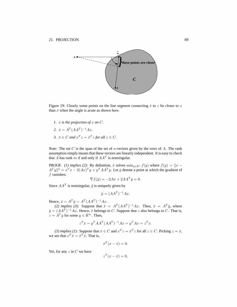
21. PROJECTION 89
x
C
x_
z
}these points are closer
Figure 19: Clearly some points on the line segment connectingx to z lie closer toxthanx when the angle is acute as shown here.
1. x is the projection ofx onC.
2. x = AT (AAT )−1Ax.
3. x ∈ C andxT z = xT z for all z ∈ C.
Note: The setC is the span of the set ofn-vectors given by the rows ofA. The rankassumption simply means that these vectors are linearly independent. It is easy to checkthatA has rankm if and only if AAT is nonsingular.
PROOF. (1) implies (2): By definition, x solvesminy∈Rn f(y) wheref(y) = ‖x −AT y‖2 = xT x− 2(Ax)T y + yT AAT y. Let y denote a point at which the gradient off vanishes:
∇f(y) = −2Ax + 2AAT y = 0.
SinceAAT is nonsingular,y is uniquely given by
y = (AAT )−1Ax.
Hence,x = AT y = AT (AAT )−1Ax.(2) implies (3): Suppose thatx = AT (AAT )−1Ax. Then, x = AT y, where
y = (AAT )−1Ax. Hence,x belongs toC. Suppose thatz also belongs toC. That is,z = AT y for somey ∈ Rm. Then,
zT x = yT AAT (AAT )−1Ax = yT Ax = zT x.
(3) implies (1):Suppose thatx ∈ C andxT z = xT z for all z ∈ C. Pickingz = x,we see thatxT x = xT x. That is,
xT (x− x) = 0.
Yet, for anyz in C we havezT (x− x) = 0.
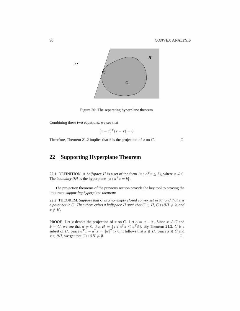
90 CONVEX ANALYSIS
x
C
x_
H
Figure 20: The separating hyperplane theorem.
Combining these two equations, we see that
(z − x)T (x− x) = 0.
Therefore, Theorem 21.2 implies thatx is the projection ofx onC. 2
22 Supporting Hyperplane Theorem
22.1 DEFINITION. AhalfspaceH is a set of the form{z : aT z ≤ b}, wherea 6= 0.Theboundary∂H is the hyperplane{z : aT z = b}.
The projection theorems of the previous section provide the key tool to proving theimportantsupporting hyperplane theorem:
22.2 THEOREM.Suppose thatC is a nonempty closed convex set inRn and thatx isa point not inC. Then there exists a halfspaceH such thatC ⊂ H, C ∩ ∂H 6= ∅, andx 6∈ H.
PROOF. Letx denote the projection ofx on C. Let a = x − x. Sincex 6∈ C andx ∈ C, we see thata 6= 0. PutH = {z : aT z ≤ aT x}. By Theorem 21.2,C is asubset ofH. SinceaT x − aT x = ‖a‖2 > 0, it follows thatx 6∈ H. Sincex ∈ C andx ∈ ∂H, we get thatC ∩ ∂H 6= ∅. 2

Measure and Integration
This chapter is devoted to integration on abstract spaces. As special cases, it covers theRiemann integral, line and surface integrals, and Stieltjes integrals.
23 Motivation
The integral introduced in elementary calculus courses is called the Riemann integral.Let’s briefly review the definition of the integral froma to b of a real-valued functionf . LetP denote a partition of the interval[a, b]:
a = x0 < x1 < x2 < · · · < xn−1 < xn = b.
Associated with this partition, is an upper estimate of the integral
U(f,P) =n∑
i=1
supxi−1≤x≤xi
f(x)(xi − xi−1)
and a lower estimate
L(f,P) =n∑
i=1
infxi−1≤x≤xi
f(x)(xi − xi−1).
Clearly,L(f,P) ≤ U(f,P).
The functionf is said to beRiemann integrableover the interval[a, b] if
supP
L(f,P) = infP
U(f,P).
The basic result regarding Riemann integration is that iff is continuous, then the Rie-mann integral exists.
There are at least three problems with the Riemann integral. The first problemis that highly discontinuous functions aren’t integrable. For example, consider thefunctionf that is one at every irrational point and is zero at every rational. Then, forevery partitionP,
U(f,P) = b− a
91

92 MEASURE AND INTEGRATION
andL(f,P) = 0.
The second problem is that one would like to be able to integrate functions whosedomain is more general than simply the reals. Of course, Riemann integrals are ex-tended to functions defined onRn, but even that is not as general as one would prefer.
The third problem is that one would often like to interchange a limit with an in-tegral. Although it is not apparent from the definition given above, it turns out thatjustifying such an interchange for Riemann integrals is difficult.
To circumvent these difficulties, the idea is to partition the range instead of thedomain (after all, the range is always the reals). Suppose first thatf is a positivefunction defined on an arbitrary setE and partition[0, n) using dyadic intervals[(k −1)/2n, k/2n). Let
Bk,n = {x ∈ E : f(x) ∈ [(k − 1)/2n, k/2n)}
denote the set of points in the domain that map into[(k− 1)/2n, k/2n). The followingsum is a lower estimate of the area underf :
n2n∑k=1
k
2nµ(Bk,n),
whereµ(Bk,n) denotes the length or, more generally, the measure ofBk,n. As nincreases, this sum increases. Therefore, it has a limit (possibly infinite) which iscalled theLebesgue integralof f overE:
∫E
f(x)µ(dx) = limn
n2n∑k=1
k
2nµ(Bk,n).
Note thatµ is a function from subsets ofE into R+. To capture the notion of beinga “measure” of the subsets,µ should possess the following properties:
1. if A1, A2, . . ., are disjoint subsets ofE, thenµ(∪nAn) =∑
n µ(An);
2. µ(∅) = 0.
A function on subsets ofE with these two properties is called ameasureonE.At this point the picture seems pretty clear. All that remains is to construct the
measureµ in the cases of interest (such as the usual notion of length onR). However,the following theorem due to Ulam shows that there aren’t many measures that can beconstructed this way.
23.1 THEOREM.If µ is a finite measure defined on all subsets of[0, 1], then thereexists a countable collection of pointsx1, x2, . . . in [0, 1] such thatµ({x1, x2, . . .}c) =0.

24. ALGEBRAS 93
Hence, there does not exist a measure defined on all subsets of[0, 1] for whichµ([a, b]) = b−a. That is, there does not exist a measure which corresponds to our ideaof length. The problem is that we have asked for too much. It is not necessary (andevidently not possible) to define our measures on all subsets ofE. The collections ofsets on which we will define our measures will be called algebras. This is the subjectof the next section.
24 Algebras
Let E be a set (generally this set will be uncountably infinite although we by no meansrequire this). We wish to assign “measures” to the sizes of various subsets ofE. Itwould be nice to assign a measure to arbitrary subsets, but as we shall see this is im-possible to do in such a way that certain natural additivity properties hold. Hence, wemust restrict our attention only to certain subsets ofE. We will call such subsetsmea-surable. If a setA is measurable, it stands to reason that its complement should alsobe measurable (and its measure should be the total measure ofE minus the measure ofA). Given a finite disjoint collection of measurable sets, it makes sense that their unionshould be measurable since the measure of the union should be the sum of the measuresof each set. Using the fact that complements of measurable sets are measurable, it iseasy to see that finite non-disjoint unions of measurable set should also be measurablesince they can be pieced together from disjoint measurable sets. Finally, it is reason-able to assume that countable unions of measurable sets should also be measurable,since the sums involved in the appropriate definition involves only positive numbersand so must either converge to a finite number or to infinity. A collection of measur-able sets will be called aσ-algebraon E. To summarize the foregoing, aσ-algebra isa non-empty collectionE of subsets ofE with the following two properties:
A ∈ E ⇒ E \A ∈ E ,
A1, A2, . . . ∈ E ⇒ ∪∞1 An ∈ E .
In other words, aσ-algebra is a collection of subsets ofE that is closed under theoperations of complementation and countable unions. It follows that aσ-algebra isclosed under finite unions, finite intersections, and countable intersections as well. Inparticular, the sets∅ andE belong to everyσ-algebra onE.
The simplestσ-algebra onE is E = {∅, E}; it is called thetrivial σ-algebra. Thelargest is the collection of all subsets; it is called thediscreteσ-algebra.
The intersection of an arbitrary family (countable or uncountable) ofσ-algebra onE is again aσ-algebra. IfC is a collection of subsets ofE, the intersection of allσ-algebras containingC is the smallestσ-algebra that containsC; it is called theσ-algebrageneratedby C and is denoted byσ(C).
If E is a metric space, then theσ-algebra generated by the collection of all opensubsets is called theBorelσ-algebraonE; it is denoted byB(E), and its elements are

94 MEASURE AND INTEGRATION
called Borel sets. Thus, every open set, every closed set, every set obtained from openand closed sets through various set operations are all Borel sets.
Monotone Class Theorem
This is a very useful theorem which simplifies the task of showing that a given col-leciton is aσ-algebra. Throughout this subsection,E is an arbitrary set.
A collectionC of subsets ofE is called aπ-systemif it is closed under finite inter-sections, that is, if
A,B ∈ C ⇒ A ∩B ∈ C.24.1
A collectionD of subsets ofE is called ad-systemonE if
(i) E ∈ D,(ii) A,B ∈ D andB ⊂ A ⇒ A \B ∈ D,(iii) (An) ⊂ D andAn ↗ A ⇒ A ∈ D.
24.2
On the last line, we wrote(An) ⊂ D to mean that(An) is a sequence of elements ofD, and we wroteAn ↗ A to mean thatA1 ⊂ A2 ⊂ · · · and∪nAn = A.
24.3 PROPOSITION.LetE be a collection of subsets ofE. Then,E is aσ-algebra onE if and only ifE is both aπ-systme and a d-system onE.
PROOF. IfE is σ-algebra then it is obviously aπ-system and a d-system. To showthe converse, suppose thatE is both aπ-system and a d-system. Now, 24.2i and 24.2iishow thatE is closed under complements. SinceA ∪ B = (Ac ∩ Bc)c, this impliesthatE is closed under unions (ifA,B ∈ E thenAc, Bc ∈ E , and thusAc ∩ Bc ∈ EsinceE is aπ-system, and hence(Ac ∩Bc)c ∈ E). This implies thatE is closed undercountable unios as well: ifA1, A2, . . . ∈ E , put
B1 = A1, B2 = A2, B3 = A3, . . . .
EachBn belongs toE by what we have just shown. Obviously,B1 ⊂ B2 ⊂ · · ·and∪nBn = cupnAn. Thus, using property 24.2iii of athe d-systemE , we see that∪nAn ∈ E . 2
The following lemma is needed in the proof of the main theorem. Its proof isobtained by checking the conditions of 24.2 one by one; we leave it as an exercise.
24.4 LEMMA. LetD be a d-system onE. Fix D ∈ D and let
|d = {A ∈ D : A ∩D ∈ D}.
Then,∩D is again a d-system.

24. ALGEBRAS 95
The following the main result of this section. It is called Dynkin’s monotome classtheorem.
24.5 THEOREM.If a d-system contains aπ-system, then it contains also theσ-algebragenerated by thatπ-system.
PROOF. LetC be aπ-system. LetD be the smallest d-system onE that containsC.We need to show thatD ⊃ σ(C). To that end, sinceσ(C) is the smallestσ-algebracontainingC, it is sufficient to show thatD is aσ-algebraFor this, it is in turn sufficientto show thatD is aπ-system (and then Proposition 24.3 implies that the d-systemD isaσ-algebra).
Fix B ∈ C and letD1 = {A ∈ D : A ∩ B ∈ D}. SinceB ∈ C ⊂ D, Lemma 24.4shows thatD1 is a d-system. Moreover,D1 ⊃ C sinceA∩B ∈ C ⊂ D for everyA ∈ Cby the fact thatC is aπ-system. SoD1 must contain the smallest d-system containingC, that is,D1 ⊃ D. In other words,A ∩B ∈ D for everyA ∈ D andB ∈ C.
Next, fix A ∈ D and letD2 = {B ∈ D : A ∩ B ∈ D}. We have just shownthatD2 ⊃ C. Moreover, by Lemma 24.4 again,D2 is a d-system. THus,D2 ⊃ D. Inother words,A ∩ B ∈ D for everyA ∈ D andB ∈ D, that is,D is aπ-system. Thiscompletes the proof. 2
Exercises:24.1 Partitions. A partition ofE is a countable disjointed collection of subsets
whose union isE. It is called a finite partition if it has only finitely manyelements.
1. Let{A,B,C} be a partition ofE. Describe theσ-algebra generatedby this partition.
2. Let C be a partition ofE. Let E be the collection of all countableunions of elements ofC. Show thatE is aσ-algebra. Show that, infact,E = σ(C).
Generally, ifC is not a partition, the elements ofσ(C) cannot be obtainedthrough such explicit constructions.
24.2 LetB andC be two collections of subsets ofE. If B ⊂ C, thenσ(B) ⊂σ(C). If B ⊂ σ(C) ⊂ σ(B), thenσ(B) = σ(C). Show these.
24.3 Borel σ-algebra onR. Show thatB(R) is generated by the collection ofall open intervals. Hint: recall that every open subset ofR is a countableunion of open intervals.
24.4 Continuation.Show that every interval ofR is a Borel set. In particular,(−∞, x), (−∞, x], (x, y], [x, y] are all Borel sets. Every singleton{x} isa Borel set.

96 MEASURE AND INTEGRATION
24.5 Show thatB(R) is also generated by any one of the following:
1. the collection of all intervals of the form(x,∞),
2. the collection of all intervals of the form(x, y],
3. the collection of all intervals of the form[x, y],
4. the collection of all intervals of the form(−∞, x],
5. the collection of all intervals of the form(x,∞) with x rational.
25 Measurable Spaces and Functions
A measurable spaceis a pair(E, E) whereE is a set andE is aσ-algebra onE. Then,the elements ofE are calledmeasurable sets. WhenE is a metric space andE = B(E),the Borelσ-algebra onE, the measurable sets are also calledBorel sets.
Let (E, E) andF,F) be measurable spaces and letf be a mapping fromE into F .Then,f is said to bemeasurablerelative toE andF if f−1(B) ∈ E for everyB ∈ F(these are the functions we wish to be able to integrate). IfE andF are metric spacesandE = B(E) andF = B(F ) andf : E 7→ F is measurable relative toE andF , tthenf is also called aBorel function.
Measurable Functions
The following proposition reduces the checks for measurability:
25.1 PROPOSITION.Let (E, E) and (F,F) be measurable spaces. In order forf :E 7→ F to be measurable relative toE and F , it is necessary and sufficient thatf−1(B) ∈ E for everyB ∈ F0 for some collectionF0 that generatesF .
PROOF. Necessity part is trivial. To prove the sufficiency, letF0 ⊂ F be such thatσ(F0) = F and suppose thatf−1(B) ∈ E for everyB ∈ F0. We need to show that,then,
F1 = {B ∈ F : f−1(B) ∈ E}
is equal toF . For this, it is sufficient to show thatF1 is aσ-algebra, sinceF1 ⊃ F0
by hypothesis andF is the smallestσ-algebra containingF0. But checking thatF1 isaσ-algebra is easy in view of the relations given in Exercise 2.1. 2

25. MEASURABLE SPACES AND FUNCTIONS 97
Borel Functions
Let E andF be metric spaces and letE andF be their respective Borelσ-algebras.Let f : E 7→ F . SinceF is generated by the open subsets ofF , in order forf to be aBorel function, it is necessary and sufficient thatf−1(B) ∈ E for every open subsetBof F ; this is an immediate corollary of the preceding proposition. In particular, iff iscontinuous, thenf−1(B) is open inE for every openB ⊂ F . Thus, every continuousfunctionf : E 7→ F is Borel measurable. The converse is generally false.
Compositions of Functions
Let (E, E), (F,F), and(G,G) be measurable spaces. Letf : E 7→ F andg : F 7→ G.Then, their compositiong ◦ f : x 7→ g(f(x)) is a mapping fromE into G. The fol-lowing proposition will be recalled by the phrase “measurable functions of measurablefunctions are measurable”.
25.2 PROPOSITION.If f is measurable relative toE andF , and if g is measurablerelative toF andG, theng ◦ f is measurable relative toE andG.
PROOF. Recall that(g ◦ f)−1(C) = f−1(g−1(C)) for everyC ⊂ G. If C ∈ G andg is measurable, thenB = g−1(C) is in F . Therefore, iff is measurable,f−1(B) =f−1(g−1(C)) is in E for everyC ∈ G. 2
Numerical Functions
By a numerical functionon E, we mean a mapping fromE into R or some subsetthereof. Such a function is said to bepositiveif all its values are inR+ and is saidto be real-valued if all its values are inR. If (E, E) is a measurable space andf is anumerical function onE, thenf is said to beE-measurableif it is measurable withrespect toE andB(R).
Let (E, E) be a measurable space and letf be a numerical function onE. UsingProposition 25.1 withF = R andF = B(R) and recalling Exercise 24.5, we see thatthe following holds.
25.3 PROPOSITION.The numerical functionf is E-measurable if and only if any oneof the following is true:
1. {x : f(x) ≤ r} ∈ E for everyr ∈ R,
2. {x : f(x) > r} ∈ E for everyr ∈ R,
3. {x : f(x) < r} ∈ E for everyr ∈ R, etc.

98 MEASURE AND INTEGRATION
25.4 COROLLARY.Suppose thatf : E 7→ F whereF is a countable subset ofR.Then,f is E-measurable if and only if{x : f(x) = a} ∈ E for everya ∈ F .
PROOF. Necessity is trivial since each singleton{a} is a Borel set. For the sufficiency,fix r ∈ R and note that{x : f(x) ≤ r} is the union of{x : f(x) = a} over alla ≤ r, a ∈ F , and therefore belongs toE since it is a countable union of the sets{x : f(x) = a} ∈ E . Thus,f is E-measurable by the preceeding proposition. 2
Positive and Negative Parts of a Function
Let (E, E) be a measurable space. Letf be a numerical function onE. Then,3
f+ = f ∨ 0, f− = −(f ∧ 0)
are called the positive part off and negative part off , respectively. Note that bothf+
andf− are positive functions and
f = f+ − f−.
25.5 PROPOSITION.The functionf is E-measurable if and only if bothf+ andf−
areE-measurable.
The proof is left as an exercise. The decompositionf = f+ − f− enables us tostate most results for positive functions only, since it is easy to obtain the correspondingresult for arbitraryf .
Indicators and Simple Functions
Let A ⊂ E. Its indicator, denoted by1A, is defined by
1A(x) ={
1 if x ∈ A,0 if x 6∈ A.
Obviously,1A is E-measurable if and only ifA ∈ E .A functionf onE is said to besimpleif it has the form
f =n∑1
ai1Ai25.6
3For a, b ∈ R we writea ∨ b for the maximum ofa andb, anda ∧ b for the minimum. The notationextends to functions:f ∨ g is the function whose value atx is f(x) ∨ g(x); similarly for f ∧ g.

25. MEASURABLE SPACES AND FUNCTIONS 99
for some integern, real numbersa1, . . . , an, and measurable setsA1, . . . , An. It isclear that, then, there exist an integerm ≥ 1, distinct real numbersb1, . . . , bm, and ameasurable partition{B1, . . . , Bm} of E such thatf =
∑m1 bi1Bi
, this latter repre-sentation is called thecanonical formof the simple functionf .
Every simple function ofE is E-measurable; this is immediate from Corollary 25.4applied to the canonical form off . Conversely, iff is E-measurable, takes only finitelymany values, and all those values are real, thenf is simple.
In particular, every constant is a simple function. Moreover, iff andg are simple,then so are
f + g, f − g, fg, f/g, f ∨ g, f ∧ g,
except that, in the case off/g one must make sure thatg is never0.
Approximations by Simple Functions
We start by constructing a sequence of simple functions that approximate the identityfunctiond from R+ into R+. For eachn ∈ N, let
dn(x) ={
k/2n if k2n ≤ x < k+1
2n , k ∈ {0, 1, . . . , n2n − 1},n if x ≥ n.
25.7
The figure below is ford2. The following lemma should be self-evident.
25.8 LEMMA. Eachdn is a simple Borel function onR+. Eachdn is right-continuousand increasing. The sequence(dn) is increasing pointwise to the functiond : x 7→ x.
The following theorem characterizes allE-measurable positive functions, and viaProposition 25.5, allE-measurable functions.
25.9 THEOREM.A positive function onE is E-measruable if and only if it is the limitof an increasing sequence of simple positive functions.
PROOF. Necessity.Let f : E 7→ R+ beE-measurable. Let thedn be defined by 25.7.Since eachdn is a measurable function fromR+ into R+, and since measurable func-tions of measurable functions are measurable, the functionfn = dn◦f isE-measurablefor eachn. Sincedn is simple, so isfn. Finally, lim fn(x) = lim dn(f(x)) = f(x)sincelim dn(y) = y for all R+. Thus,f is the limit of the sequence(fn) of simplepositive functions andf1 ≤ f2 ≤ · · · sinced1 ≤ d2 ≤ · · ·.
Sufficiency.Let f1 ≤ f2 ≤ · · · be simple and positive and letf = lim fn. Now, foreachx ∈ E andr ∈ R, we havef(x) ≤ r if and only if fn(x) ≤ r for all n; thus,
{x ∈ E : f(x) ≤ r} = ∩∞n=1{x ∈ E : fn(x) ≤ r}
for eachr ∈ R. Since thefn are simple (and therefore measurable), each factor onthe right side belongs toE and, therefore, so does the intersection. Hence,f is E-measurable by Proposition 25.3. 2

100 MEASURE AND INTEGRATION
Limits of Sequences of Functions
Let (E, E) be a measurable space and let(fn) be a sequence of numerical functions onE.
25.10 THEOREM.Suppose that eachfn is E-measurable. The, each one of
inf fn, sup fn, lim inf fn, lim sup fn
is againE-measurable. Moreover, iflim fn exists, then it isE-measurable.
PROOF. Forx ∈ E andr ∈ R, we haveinf fn(x) ≥ r if and only if fn(x) ≥ r for alln. Thus, for eachr ∈ R,
{x ∈ E : inf fn(x) ≥ r} = ∩n{x ∈ E : fn(x) ≥ r}.
Now, {x : fn(x) ≥ r} ∈ E for eachn by the measurability offn, and therefore the in-tersection on the right side belongs toE sinceE is closed under countable intersections.Thus,inf fn is E-measurable by Proposition 25.3.
The proof thatsup fn is E-measurable follows via similar reasoning upon notingthat
{x ∈ E : sup fn(x) ≤ r} = ∩n{x ∈ E : fn(x) ≤ r}.
It follows from these that
lim inf fn = supm
infn≥m
fn, lim sup fn = infm
supn≥m
fn
are bothE-measurable. Finally,lim fn exists if and only iflim inf fn = lim sup fn,and thenlim fn is the common limit; so, it must beE-measurable. 2
Monotone Classes of Functions
Often we are interested in showing that a certain property holds for all measurablefunctions. The following are useful in such quests.
LetM be a collection of positive functions onE. Then,M is called amonotoneclass of functionsprovided that
(i) 1 ∈M,(ii) f, g ∈M, anda, b ∈ R+ ⇒ af + bg ∈M,(iii) (fn) ⊂M, andfn ↗ f ⇒ f ∈M.
25.11
The following is called the monotone class theorem for functions.
25.12 THEOREM.LetM be a monotone class of functions onE. Suppose that1A ∈M for everyA ∈ C for someπ-systemC that generates theσ-algebraE . Then,M

25. MEASURABLE SPACES AND FUNCTIONS 101
includes all positiveE-measurable functions and all boundedE-measurable functions.
PROOF. We start by showing that1A ∈M for everyA ∈ E . To this end, let
D = {A ∈ E : 1A ∈M}.
Using the properties 25.11 ofM, it is easy to check thatD is a d-system. Moreover,D ⊃ C by hypothesis. Thus, by Dynkin’s monotone class theorem,D ⊃ σ(C) = E . Inother words,1A ∈M for everyA ∈ E .
Consequently, in view of property 25.11(ii),M includes all simpleE-measurablefunctions.
Let f be a positiveE-measurable function. By Theorem 25.9, there exists a se-quence of positive simple functionsfn ↗ f . Since eachfn in inM by the preceedingstep, 25.11(iii) implies thatf is inM.
2
Notation
We shall writef ∈ E to mean thatf is anE-measurable function. Thus,E standsboth for aσ-algebra and for the collection of all numerical functions measurable withrespect to it. Furthermore, we shall use the notation
F+ = {f ∈ F : f ≥ 0}
for any collection ofF of numerical functions. Thus, in particular,E+ is the collectionof all positiveE-measurable functions.
Exercises:
25.1 Trace spaces.Let (E, E) be a measurable space and letD ⊂ E be fixed.Show that
D = {A ∩D : A ∈ E}
is aσ-algebra onD. Then,D is called the trace ofE onD, and(D,D) iscalled the trace of(E, E) onD.
25.2 σ-algebra generated by a function.Let E be a set and let(F,F) be ameasurable space, Letf be a mapping fromE into F and set
f−1(F) = {f−1(B) : B ∈ F}.
Use Exercise 2.1 to show thatf−1(F) is aσ-algebra onE; it is called theσ-algebra onE generated byf . It is the smallestσ-algebra onE such thatf is measurable relative to it andF .

102 MEASURE AND INTEGRATION
25.3 Product spaces.Let (E, E) and(F,F) be measurable spaces. A rectangleA × B is said to be measurable ifA ∈ E andB ∈ F . Show that thecollection of all measurable rectangles form aπ-system. Theσ-algebra onE × F generated by thatπ-system is denoted byE ⊗ F and is called theproductσ-algebra. Further,(E×F, E ⊗F) is called the product of(E, E)and(F,F), and is denoted by(E, E) × (F,F) also. If (E, E) = (F,F),then it is usual to writeE2 for E × F andE2 = E ⊗ F . In particular,(R2,B(R2)) = (R,B(R)) × (R,B(R)), and by an obvious extension,(Rn,B(Rn)) = (R,B(R))× · · · × (R,B(R)), n times.
25.4 Continuation. Let (E, E), (F,F), (G,G) be measurable spaces. Letf : E 7→ F be measurable relative toE andF , and letg : E 7→ Gbe measurable relative toE andG. Then,
h(x) = (f(x), g(x)), x ∈ E,
defines a mapping fromE into F ×G. Show thath is measurable relativeto E andF ⊗G.
In particular, a functionf : E 7→ Rn is measurable relative toE andB(Rn) if and only if its coordinates are measurable relative toE andB(R); recall that the coordinates off are the functionsf1, . . . , fn suchthatf(x) = (f1(x), . . . , fn(x)), x ∈ E.
25.5 Discrete spaces.A measurable space(E, E) is said to bediscreteif E iscountable andE is theσ-algebra of all subsets ofE. Then, show that everynumerical function ofE is E-measurable.
25.6 Suppose thatE is generated by a countable partition ofE. Show that, then,a numerical function onE is E-measurable if and only if it is constant overeach member of that partition.
25.7 Approximation by simple functions.Show that a numerical function ofE is E-measruable if and only if it is the limit of a sequence of simplefunctions.
25.8 Arithmetic operations.Let f andg be E-measurable. Show that, then,each one of
f + g, f − g, f · g, f/g, f ∨ g, f ∧ g
is E-measurable provided that it be well-defined.
25.9 Functions onR. Let f : R 7→ R+ be increasing. Show that it is a Borelfunction.
25.10 Step functions.A function f : R 7→ R is called a step function if it hasthe form
f =∞∑1
ai1Ai

26. MEASURES 103
where eachAi is an interval. Show that every suchf is a Borel function.
25.11 Right-continuous functions.Show that every right-continuous functionf : R 7→ R is Borel measurable. SImilarly, every left-continuous functionis Borel. Hint for right-continuousf : definedn(x) = (k + 1)/2n ifk/2n ≤ x < (k + 1)/2n for somek = 0, 1, 2, . . . for n = 1, 2, . . .. Showthat dn is Borel. Letfn(x) = f(dn(x)). Show that eachfn is a stepfunction, and show thatfn → f asn →∞.
26 Measures
Let E, E) be a measurable space. Ameasureon (E, E) is a mappingµ : E 7→ R+ suchthat
1. µ(∅) = 0 ,
2. µ(∪nAn) =∑
n µ(An) for every disjointed sequence(An) ⊂ E .
The latter condition is calledcountable additivity.A measure spaceis a triplet(E, E , µ) whereE is a set,E is aσ-algebra onE, and
µ is a measure on(E, E).
26.1 PROPOSITION.Let µ be a measure on(E, E). Then, the following hold for allmeasurable setsA,B, andAn, n ≥ 1:
Finite additivity: A ∩B = ∅ implies thatµ(A ∪B) = µ(A) + µ(B).
Monotonicity: A ⊂ B implies thatµ(A) ≤ µ(B).
Sequential continuity: An ↗ A implies thatµ(An) ↗ µ(A).
Boole’s inequality: µ(∪nAn) ≤∑
n µ(An).
PROOF. Finite additivity is a particular instance of the countable additivity ofµ: takeA1 = A, A2 = B, A3 = A4 = · · · = ∅. Monotonicity follows from it and thepositivity of µ: if A ⊂ B,
µ(B) = µ(A) + µ(B \A) ≥ µ(A)
sinceµ(B\A) ≥ 0. Sequential continuity follows from (and is equivalent to) countableadditivity: suppose thatAn ↗ A; then,
B1 = A1, B2 = A2 \A1, B3 = A3 \A2, · · ·

104 MEASURE AND INTEGRATION
are disjoint, their union isA, and the union of the firstn is An; hence, the sequence ofnumbersµ(An) increases by the monotonicity ofµ, and
limµ(An) = lim µ(∪n1Bi) = lim
n
n∑1
µ(Bi) =∞∑1
µ(Bi) = µ(∪∞1 Bi) = µ(A).
Finally, Boole’s inequality follows from the observation that
µ(A ∪B) = µ(A) + µ(B \A) ≤ µ(A) + µ(B).
2
Arithmetic of Measures
Let (E, E) be a measurable space. Ifµ is a measure on it and ifc ≥ 0 is a constant,thencµ is again a measure. Ifµ andν are measures on(E, E), so isµ+ν. If µ1, µ2, . . .are measures, then so isµ =
∑µm: it is obvious thatµ(∅) = 0, and ifA1, A2, . . . are
disjoint then
µ(∪nAn) =∑m
µm(∪nAn)
=∑m
∑n
µm(An)
=∑
n
∑m
µm(An)
=∑
n
µ(An),
where the crucial step (where the order of summation is changed) is justified by theelementary fact that ∑
m
∑n
amn =∑
n
∑m
amn
if amn ≥ 0 for all m,n.
Finite, σ-finite, Σ-finite measures
Let µ be a measure on(E, E). It is said to befinite if µ(E) < ∞. It is called aprobability measureif µ(E) = 1. It is said to beσ-finite if there exists a measurablepartition(En) of E such thatµ(En) < ∞ for eachn. It is said to beΣ-finite if thereexist finite measuresµ1, µ2, . . . such thatµ =
∑µn. Note that every finite measure
is trivially σ-finite, everyσ-finite measure isΣ-finite. The converses are false (seeExercise 26.4).

26. MEASURES 105
Specification of Measures
It is generally difficult to specifyµ(A) for eachA, simply because there are too manyAin a σ-algebra. The following proposition is helpful in reducing the task to specifyingµ(A) for thoseA belonging to aπ-system that generates the givenσ-algebra.
26.2 PROPOSITION.Let µ and ν be measures on(E, E). Suppose thatµ(E) =ν(E) < ∞, and thatµ andν agree on aπ-system generatingE . Then,µ = ν.
PROOF. LetC be aπ-system withσ(C) = E . Suppose thatµ(A) = ν(A) for everyA ∈ C. We need to show that, then,µ(A) = ν(A) for everyA ∈ E . This amounts toshowing that
D = {A ∈ E : µ(A) = ν(A)}containsE . Now,D ⊃ C by hypothesis, and it is straightforward to check thatD is ad-system. Thus, by Dynkin’s monotone class theorem,D ⊃ σ(C) = E . 2
26.3 COROLLARY.LEt µ andν be probability measures onR,B(R)). Then,µ = νif and only if, for everyx ∈ R,
µ((−∞, x]) = ν((−∞, x]).
PROOF. The collectionC of all intervals of the form(−∞, x] is aπ-system generatingB(R). THus, the preceding proposition applies to prove sufficiency. Necessity is trivial.2
The following proposition extends 26.2 toσ-finite measures.
26.4 PROPOSITION.Let µ andν beσ-finite measures on(E, E). Suppose that theyagree on aπ-systemC generatingE . Suppose further that there is a partition(En) ofE such thatEn ∈ C andµ(En) = ν(En) < ∞ for everyn. Then,µ = ν.
PROOF. For eachn, define the measuresµn andνn on (E, E) by
µn(A) = µ(A ∩ En), νn(A) = ν(A ∩ En), A ∈ E .
SInceEn ∈ C, and sinceA ∩ En ∈ C for everyA ∈ C, we have
µn(A) = µ(A ∩ En) = ν(A ∩ En) = νn(A) for A ∈ C.
And, by hypothesis,µn(E) = µ(E) = ν(E) = νn(E) < ∞. Thus, the last proposi-tion applies to show thatµn = νn for eachn. This completes the proof sinceµ =
∑µn
andν =∑
νn. 2

106 MEASURE AND INTEGRATION
Image of Measure
Let (E, E) and(F,F) be measurable spaces. Letµ be a measure on(E, E) and letf : E 7→ F be measurable relative toE andF . Then,
µ ◦ f−1(B) = µ(f−1(B)), B ∈ F ,26.5
is well-defined sincef−1(B) ∈ E for eachB ∈ F . It is easy to check thatν = µ◦f−1
is a measure on(F,F). It is called theimage ofµ underf .
Almost Everywhere
Often we face situations where a certain statement is true for everyx ∈ E0 andE0 isalmost the same asE in the sense thatE0 ∈ E andµ(E \E0) = 0. In that case, we saythat the statement is true foralmost everyx in E or that the statement is true almosteverywhere.
Incidentally, a setN ⊂ E is said to be neglibible if there is anA ∈ E such thatN ⊂ A andµ(A) = 0. So, a statement holds almost everywhere if and only if it failsonly over a neglibible set.
EXAMPLES.
26.6 Dirac measure.Let (E, E) be a measurable space. Fixx ∈ E. Define
δx(A) ={
1 if x ∈ A0 if x 6∈ A
for eachA ∈ E . Then,δx is a measure on(E, E). It is called theDirac measuresittingatx.
26.7 Counting measures.Let (E, E) be a measurable space and letD be a countablesubset ofE. Define a measureν on (E, E) by
ν =∑x∈D
δx.
Note thatν(A) is the number of points inA ∩D. Such measures are called countingmeasures.
26.8 Discrete measure spaces.Let E be countable andE be the collection of allsubsets ofE. Specifying a measure on(E, E) is equivalent to assigning a numberm(x) in R+ to each pointx in E and then letting
µ(A) =∑x∈A
m(x), A ∈ E .
26. MEASURES 107
Then,m is called the mass function corresponding toµ. In particular, ifE = {1, 2, . . . , n},every measureµ on (E, E) can be regarded a a vector inRn.
26.9 Purely atomic measures.Let (E, E) be a measurable space, letD be a countablesubset ofE, and letm(x) be a positive number for eachx ∈ D. Define
µ(A) =∑x∈D
m(x)δx(A), A ∈ E .
Then,µ is a measure on(E, E). It puts the massm(x) at the pointx, and there areonly countable many pointsx like that. Suchµ are said to be purely atomic, the pointsx with µ({x}) > 0 are called the atoms ofµ.
26.10 Lebesgue measures.A measureµ on (R,B(R)) is called theLebesgue measureon R if µ(A) is the length ofA for every intervalA. The collectionC of all intervalsform a π-system that generatesB(R) and thus, by Proposition 26.4, there can be atmost one such measure. The whole point of all measure theory is the following theoremwhich, unfortunately, we don’t prove.
26.11 THEOREM.There exists a measure on(R,B(R)) which assigns to each intervalA its length.
It is impossible to displayµ(A) explicity for each Borel setA, but countable ad-ditivity and various properties list in Proposition 26.1 enable us to figureµ(A) out formost reasonable setsA. For instance,µ({x}) = 0 for everyx ∈ R, µ(A) = 0 forevery countable setA ⊂ R, µ(A) = 0 for the cantor setA, and so on. Of course, thereare many sets with strictly positive measure.
Similarly, Lebesgue measure onR2 is the “area” measure, Lebesgue measure onR3 is the “volume” measure, and so on. All Lebesgue measures onR, R2, R3, etc. areσ-finite.
More generally, given an intervalE ⊂ R, it makes sense to talk of Lebesgue mea-sure on(E,B(E)); this is the restriction of Lebesgue measure onR to the trace space(E,B(E)). Similarly, one can talk of Lebesgue measure on a domain inR2 or on a do-main inRn. In all cases we shall useλn to denote the Lebesgue measure on a domainin Rn.
Exercises:26.1 Show thatD in the proof of 26.2 is a d-system.
26.2 Restrictions.Let (E, E , µ) be a measure space. LetD ∈ E and letD ={A ∈ E : A ⊂ D}. Then,(D,D) is the trace of(E, E) on D. Defineν(A) = µ(A) for A ∈ D. Then,ν is a measure on(D,D); it is called therestrictionof µ to D.

108 MEASURE AND INTEGRATION
26.3 Uniform distribution. Let D ⊂ R be an interval of finite length. Letµ(B) = λ1(B)/λ1(D) for Borel subsetsB of D. Show thatµ is a prob-ability measure on(D,D) whereD = B(D). It is called theuniformdistributiononD.
26.4 Σ-finiteness. Let E = {a, b} with the discreteσ-algebra, and defineµ({a}) = 0, µ({b}) = +∞. Show that this defines aΣ-finite measureµ that is notσ-finite.
26.5 Atoms, atomic measures, diffuse measures.Let (E, E) be such the{x} ∈E for everyx ∈ E. A point x is said to be anatom for the measureµif µ({x}) > 0. If µ has no atoms, then it is said to bediffuse. If µ putsno mass outside the set of its atoms, then it ispurely atomic. In general,µ will have some atomic part and some diffuse part. This is to show thisdecomposition.
1. Letµ be finite. Show that it has at most countably many atoms. Hint:let D be the set of atoms, note thatD = ∪nDn whereDn = {x :µ({x}) ∈ [1/n, 1/(n− 1)), n = 1, 2, . . .. Use the finiteness ofµ toconclude that eachDn is a finite set, and therefore, thatD must becountable.
2. Letµ beΣ-finite. Show that it has at most countably many atoms.
3. LetD be the set of atoms of aΣ-finite measureµ. Define
ν(A) = µ(A ∩D), λ(A) = µ(A ∩Dc), A ∈ E .
Then,ν is purely atomic,λ is diffuse, and
µ = ν + λ.
27 Integration
Let (E, E) be a measurable space. Recall thatE stands also for the collection of allE-measurable functions and thatE+ is the sub-collection consisting of positiveE-measurable functions. Given a measureµ on (E, E), our aim is to define the “integralof f with respect toµ” for all reasonable functionsf in E . We shall denote it by any ofthe following:
µf =∫
E
µ(dx)f(x) =∫
E
fdµ.
When E is an interval ofR and f is continuous andµ is the Lebesgue measure,the integral will coincide with the usual Riemann integral off on E. WhenE ={1, . . . , n} andE is the discreteσ-algebra, every measureµ is specified by a row vec-tor (µ1, . . . , µn) with µi denotingµ({i}), and every functionf ∈ E corresponds to acolumn vector(f1, . . . , fn) with fi = f(i); in this case the integralµf will coincide

27. INTEGRATION 109
with the product of the row vector(µ1, . . . , µn) with the column vector with entiresf1, . . . , fn. As this last case illustrates, it is best to think of the integral as a product.After we define it, we shall show that it has the properties of products.
Definition of the Integral
We define the integralµf in three steps: first for simple positivef , then forf ∈ E+,finally for reasonablef ∈ E .
Step 1. Let f be a nonnegative simple function. If its cannonical form isf =∑n1 ai1Ai
, then we define
µf =n∑1
aiµ(Ai).27.1
Step 2. Let f ∈ E+. Let (dn) be defined by 25.7 and recall from the proof ofTheorem 25.9 thatlim dn ◦ f = f . Now, for eachn, the functiondn ◦ f is simple andpositive, and the integralµ(dn ◦ f) is defined by the preceding step. We shall show inthe remarks below that the numbersµ(dn ◦f) form an increasing sequence, and hence,limµ(dn ◦ f) exists (it may be+∞). Sincef = lim dn ◦ f , we define
µf = lim µ(dn ◦ f).27.2
Step 3.Let f ∈ E be arbitrary. Then,f+ andf− belong toE+, and their integralsare defined by the preceding step. Noting thatf = f+ − f−, we define
µf = µf+ − µf−27.3
provided that at least one term on the right is finite. Otherwise, ifµf+ = µf− = +∞,thenµf does not exist.
REMARKS: (a) Formula 27.1 holds for nonnegative simple functions even when∑n1 ai1Ai
is not the canonical representation forf :
f =n∑1
ai1Ai=
m∑1
bj1Bj⇒ µf =
n∑1
aiµ(Ai) =m∑1
bjµ(Bj).
This is easy to check using the finite additivity ofµ.(b) If f andg are nonnegative simple functions anda, b ∈ R+, thenaf + bg is
again a nonnegative simple function, and
µ(af + bg) = a µf + b µg.
This can be checked using the preceding remark.(c) If f is a nonnegative simple function, then 27.1 shows thatµf ≥ 0 (it can be
+∞).(d) If f andg are nonnegative simple functions andf ≤ g, then the preceding two
remarks applied tof andg − f show thatµf ≤ µg.(e) In Step 2 of the definition, we haved1 ◦ f ≤ d2 ◦ f ≤ · · · and the preceding
remark shows thatµ(d1 ◦ f) ≤ µ(d2 ◦ f) ≤ · · · as claimed.

110 MEASURE AND INTEGRATION
Integral over a Set
Let f be a measurable function andA a measurable set. Then,f1A ∈ E . The integralof f overA is defined to be the integral off1A; it exists if and only ifµ(f1A) exists.The following notations are used for it:
µ(f1A) =∫
A
µ(dx)f(x) =∫
A
fdµ.27.4
Integrability
A function f ∈ E is said to beintegrableif µf exists and is a finite number. Thus,f ∈ E is integrable if and only ifµf+ < ∞ andµf− < ∞, or equivalently, if andonly if µ|f | < ∞ (note that|f | = f+ + f−).
Elementary Properties
Here are some familiar properties of the integrals. A few others are put into the exer-cises.
27.5 PROPOSITION.(a) Positivity. If f ∈ E+, thenµf ≥ 0.(b) For f ∈ E+, µf = 0 if and only iff = 0 almost everywhere.(c) Monotonicity. If f, g ∈ E+ andf ≤ g, thenµf ≤ µg. If f, g ∈ E andf, g are
integrable, andf ≤ g, thenµf ≤ µg.(d) Finite additivity over sets.Let f ∈ E+. If {A1, . . . , Am} is a measurable
partition ofA ∈ E , then ∫A
fdµ =m∑
i=1
∫Ai
fdµ.27.6
PROOF. (a) Iff ≥ 0, then the definition ofµf yieldsµf ≥ 0.(c) If 0 ≤ f ≤ g, thendn ◦ f ≤ dn ◦ g and so
µ(dn ◦ f) ≤ µ(dn ◦ g)
by the monotonicity of integration for simple functions. Now, the left-hand side con-verges toµf and the right-hand side converges toµg. Henceµf ≤ µg. The generalcase is similar.
(b) Linearity for simple functions and monotonicity imply the following chain ofinequalities:
0 ≤ 1n
µ({x : f(x) ≥ 1n}) =
1n
µ(1f≥ 1n) = µ(
1n
1f≥ 1n) ≤ µ(f1f≥ 1
n) ≤ µf = 0.

27. INTEGRATION 111
Since the two ends of this chain of inequalities are equal, it follows that all the inequal-ities are in fact equalities. Hence,
µ({x : f(x) ≥ 1/n}) = 0 ∀n
and so{x : f(x) > 0} = ∪n{x : f(x) ≥ 1/n}.
Taking the measure of both sides, we get
0 ≤ µ({x : f(x) > 0}) ≤∑
n
µ({x : f(x) ≥ 1/n}) = 0.
Again, equating this anchored chain of inequalities, we see thatf = 0 a.e.(d) Fix f ∈ E+. Let A1, . . . , Am ∈ E be disjoint with unionA. If f is simple, 27.6
is immediate from Remark b applied to the simple functionsf1A1 , . . . , f1Am whosesum isf1A. Applying this to simple functionsdn ◦ f , we see that
m∑1
µ(1Aidn ◦ f) = µ(1Adn ◦ f).
Note that1B(x)dn ◦ f(x) = dn(1B(x)f(x)) for eachx by the way the functiondn isdefined. Putting this observation into the preceding expression and lettingn → ∞ weobtain
m∑1
µ(f1Ai) =
m∑1
limn
µ(dn ◦ (f1Ai))
= limn
m∑1
µ(dn ◦ (f1Ai))
= limn
µ(dn ◦ (f1A))
= limn
µ(f1A),
where the interchange of the limit and the sum is justified by the finiteness ofm. 2
Monotone Convergence Theorem
This is the key result in the theory of integration. It allows interchanging the order oftaking limits and integrals under reasonable conditions.
27.7 THEOREM.Let (fn) ⊂ E+ be increasing. Then,
µ(lim fn) = lim µfn.

112 MEASURE AND INTEGRATION
PROOF. Letf = lim fn; it is well-defined sincef1 ≤ f2 ≤ · · · and is positive andE-measurable. So,µf is well-defined. By the monotonicity of integration,µf1 ≤ µf2 ≤· · · ≤ µf . Thereforelim µfn exists and
limn
µfn ≤ µf.
It remains to show thatlimn µfn ≥ µf . This is accomplished in steps.Step 1. Ifb ∈ R+, B ∈ E , andf(x) > b for x ∈ B, thenlimn µ(fn1B) ≥ bµ(B).First, note that{f1 > b} ⊂ {f2 > b} ⊂ · · · and that
∪n{fn > b} = {x : fn(x) > b for somen} = {f > b}.
PutBn = {fn > b} ∩B. Then,Bn ↗ and∪nBn = {f > b} ∩B = B. Thus,
limn
µ(Bn) = µ(B)27.8
by the sequential continuity ofµ under increasing limits. Now, note that
fn1B ≥ fn1Bn≥ b1Bn
,
and so the monotonicity of integration yields that
µ(fn1B) ≥ µ(b1Bn) = bµ(Bn).
Taking limits on both sides and using 27.8, we get
lim µ(fn1B) ≥ bµ(B).27.9
Step 2. The same inequality holds even iff(x) ≥ b for x ∈ B.Forb = 0, this is trivial. Forb > 0, apply Step 1 withb−ε to see thatlimn µ(fn1B) ≥
(b−ε)µ(B). Sinceε is arbitrary, we can let it go to zero to obtain the desired inequality.Step 3. Ifg is a simple function andg ≤ f , thenlimn µfn ≥ µg.Let
∑m1 bi1Bi
denote the canonical representation forg. Then, our assumptionsimply thatf(x) ≥ g(x) = bi for x ∈ Bi. Hence, we may apply the result of Step 2 toconclude that
limn
µ(fn1Bi) ≥ biµ(Bi) i = 1, . . . ,m.
Hence, by Proposition 27.5d applied to the functionfn, we see that
limn
µfn = limn
m∑1
µ(fn1Bi)
=m∑1
lim µ(fn1Bi)
≥m∑1
biµ(Bi) = µg.

27. INTEGRATION 113
Step 4.limn µfn ≥ µf .Putg = dm ◦ f . Step 3 applied with thisg yields limn µfn ≥ µ(dm ◦ f). Letting
m →∞ we get the desired result. 2
A particular consequence of the monotone convergence theorem is that, in defini-tion 27.2, the special sequence(dn ◦ f) can be replaced by any sequence(fn) ⊂ E+
increasing tof .
Linearity of Integration
27.10 PROPOSITION.If f, g ∈ E+ anda, b ∈ R+, then
µ(af + bg) = aµf + bµg.
The same holds for arbitraryf, g ∈ E and a, b ∈ R provided that both sides arewell-defined. It holds, in particular, iff andg are integrable.
PROOF. Iff, g are simple, the result is established by direct checking as was remarkedin b. Forf, g ∈ E+, anda, b ∈ R+, choose(fn) and(gn) to be sequences of simplepositive functions increasing tof andg, respectively. Then,
µ(afn + bgn) = aµfn + bµgn,
andafn + bgn ↗ af + bg, fn ↗ f , gn ↗ f . Taking limits on both sides and using themonotone convergence theorem completes the proof. Iff, g ∈ E are arbitrary, writef = f+ − f− andg = f+ − g− and go through the same steps. 2
Fatou’s Lemma
This gives a useful inequlaity for arbitrary sequences of positive measurable functions.
27.11 LEMMA.Let (fn) ⊂ E+. Then,µ(lim inf fn) ≤ lim inf µfn.
PROOF. Definegm = infn≥m fn. Then, lim inf fn is the limit of the increasingsequence(gm) ⊂ E+, and thus
µ(lim inf fn) = µ(lim gm) = lim µgm
by the monotone convergence theorem. On the other hand,gm ≤ fn for all n ≥ m,which yieldsµgm ≤ µfn for all n ≥ m, which in turn means thatµgm ≤ infn≥m µfn.Hence, as needed,
limµgm ≤ limm
infn≥m
µfn = lim inf µfn.
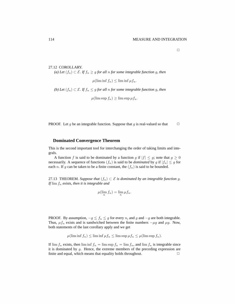
114 MEASURE AND INTEGRATION
2
27.12 COROLLARY.(a) Let(fn) ⊂ E . If fn ≥ g for all n for some integrable functiong, then
µ(lim inf fn) ≤ lim inf µfn.
(b) Let(fn) ⊂ E . If fn ≤ g for all n for some integrable functiong, then
µ(lim sup fn) ≥ lim sup µfn.
PROOF. Letg be an integrable function. Suppose thatg is real-valued so that 2
Dominated Convergence Theorem
This is the second important tool for interchanging the order of taking limits and inte-grals.
A function f is said to be dominated by a functiong if |f | ≤ g; note thatg ≥ 0necessarily. A sequence of functions(fn) is said to bedominatedby g if |fn| ≤ g foreachn. If g can be taken to be a finite constant, the(fn) is said to be bounded.
27.13 THEOREM.Suppose that(fn) ⊂ E is dominated by an integrable functiong.If lim fn exists, then it is integrable and
µ(limn
fn) = limn
µfn.
PROOF. By assumption,−g ≤ fn ≤ g for everyn, andg and−g are both integrable.Thus,µfn exists and is sandwiched between the finite numbers−µg andµg. Now,both statements of the last corollary apply and we get
µ(lim inf fn) ≤ lim inf µfn ≤ lim sup µfn ≤ µ(lim sup fn).
If lim fn exists, thenlim inf fn = lim sup fn = lim fn, andlim fn is integrable sinceit is dominated byg. Hence, the extreme members of the preceding expression arefinite and equal, which means that equality holds throughout. 2

27. INTEGRATION 115
If (fn) ⊂ E is bounded, say by the constantb, and if the measureµ is finite, then wecan takeg = b in the preceding theorem. The resulting corollary is called theboundedconvergence theorem:
27.14 THEOREM.Let (fn) ⊂ E be bounded. Suppose thatµ is finite. If lim fn exists,then
µ(limn
fn) = limn
µfn.
27.15 EXAMPLE. Let(E, E) = (R+,B(R+)) and letfn be the sequence of functionsshown in Figure??. Note that the functions are not monotone and there is no integrablefunction that dominates them. Also,µfn = 1 for all n and solim µfn = 1, whereas,lim fn = 0 and soµ lim fn = 0.
Related Documents


