Mathematical Methods in Composing Melodies

Lynchburg CollegeDigital Showcase @ Lynchburg College

Undergraduate Theses and Capstone Projects

Spring 4-1-2007

Mathematical Methods in Composing MelodiesThomas BrownLynchburg College

Follow this and additional works at: https://digitalshowcase.lynchburg.edu/utcp

Part of the Composition Commons, Dynamic Systems Commons, Fine Arts Commons,Musicology Commons, Music Theory Commons, Numerical Analysis and Computation Commons,Other Applied Mathematics Commons, Other Music Commons, Partial Differential EquationsCommons, and the Special Functions Commons

This Thesis is brought to you for free and open access by Digital Showcase @ Lynchburg College. It has been accepted for inclusion in UndergraduateTheses and Capstone Projects by an authorized administrator of Digital Showcase @ Lynchburg College. For more information, please [email protected].

Recommended CitationBrown, Thomas, "Mathematical Methods in Composing Melodies" (2007). Undergraduate Theses and Capstone Projects. 42.https://digitalshowcase.lynchburg.edu/utcp/42

Mathematical Methods in Composing Melodies

Thomas Brown

Senior Honors Project

Submitted in partial fulfillment of the graduation requirements of the Westover Honors Program

Westover Honors Program

April, 2007

Dr. Chris Gassler

Dr. Kevin Peterson, Committee Chair

Dr. Nancy Cowden,Westerner Honors Representative

TABLE OF CONTENTS

Table of Figures.......................................................................................................................... .. 3

Abstract....................................................................................................................................... .. 4

Introduction................................................................................................................................. .5

Methods....................................................................................................................................... 12

Results......................................................................................................................................... 17

1. Random content.......................................................................................................... 17

2. Sierpinski music......................................................................................................... 18

3. Chaotic unimodal quadratic maps.............................................................................. 19

4. Linear distribution...................................................................................................... 22

5. Cauchy distribution.................................................................................................... 24

6. Fractal music............................................................................................................... 25

7. Random walk.............................................................................................................. 27

Discussion and Conclusions....................................................................................................... 28

Bibliography................................................................................................................................ 31

Appendix A.................................................................................................................................. 33

Appendix B.................................................................................................................................. 40

Appendix C................................................................................................................................. 43

Appendix D................................................................................................................................... 44

Table of Figures

Figure 1: The Mandelbrot Set.................................................................................................... ...8

Figure 2: The Mandelbrot set magnified at 1,048,800 times figure 1....................................... ...8

Figures 3-8: Different stages in examining the chaotic behavior of a quadratic unimodal map ..10

Figure 9: Steps in constructing a Sierpinski triangle.................................................................. .13

Figure 10: Melodic representation of random content.............................................................. ..17

Figure 11: Melodic representation of Sierpinski music............................................................. ..18

Figure 12: Melodic representation of chaotic unimodal quadratic maps with lambda set at 3.8.20

Figure 13: Melodic representation of chaotic unimodal quadratic maps with lambda set at 3.9.20

Figure 14: Melodic representation of chaotic unimodal quadratic maps with lambda set at 4.0.20

Figure 15: Melodic representation of a linear distribution......................................................... .23

Figure 16: Melodic representation of a Cauchy distribution with alpha set at 5..........................24

Figure 17: Melodic representation of fractal music................................................................... ..25

Figure 18: Melodic representation of a random walk................................................................ ..27

4

Abstract

This thesis, “Mathematical Methods in Composing Melodies,” explores the different

ways in which mathematics can be used to create music. Some research has been done in this

field already. Richard F. Voss and John Clarke used fractals and different frequencies of noise to

create music. The Greek composer Iannis Xenakis used Markovian Stochastic trees to create

some of his compositions. Explored in this thesis are seven different methods to compose

melodies. After compiling the different melodies, they were categorized by different musical

periods based on the musical characteristics found in the melody. This thesis differs from other

research that deals with the relationship between music and math. Contrary to previous

investigations, the purpose of this thesis is to take something purely mathematical and make

music from it. From the methods used, the music created from formulas for fractal music and

chaotic unimodal quadratic maps created the most musically interesting melodies.

5

Introduction

The relationship between Mathematics and Music has been studied for centuries. There

have also been several methods employed over the past four hundred years that use math to

create music. Most of these methods appeared in the 20th century. There are many composers

and theorists that create music based on mathematics or analyze music and discover that it has

mathematical properties. My thesis concentrates on creating musical melodies by using

mathematical principles and formulas. In addition to creating music, the melodies were also

analyzed in order to determine what style of music the melodies resemble. This method was

used to determine if these melodies are in fact musical or just random noise.

Leon Harkleroad’s book The Math Behind the Music (2006) provides a great

introduction to the relationship between math and music. Harkleroad presents the basic

principles of physics behind music including the Pythagorean ratios that create the basic intervals

between notes (pp. 10-13), an explanation of overtones (pp. 16-19), and different tuning systems

that have been used in creating musical scales (pp. 21-32). His book also contains information

on how to vary an already existing melody by using one or a combination of the following

methods: transposition (creating a new melody by moving each note of the original melody by

the same interval), inversion (creating a new melody by using the opposite, or inverse, intervals

between the notes of the original melody), and retrograde (creating a new melody by reversing

the order of the notes of the original melody) (pp. 33-54). He explains how a similar idea to

transpositions, inversions, and retrogrades were used to create different melodies in the practice

of ringing church bells in the 17th century (pp. 60-69).

Harkleroad also discusses several methods of creating music that involve probability (pp.

71-91). These methods include random chance, as in rolling dice, and Markov chains. Markov

chains are chains of random functions, also known as stochastic processes, that deal with the

probability of moving from one random variable to another (Xenakis, 1972, p. 73). In terms of

music this would mean starting with a random note and determining what the probability is that

you could get to another note or series of notes.

Greek Composer Iannis Xenakis used Markov chains to create some of his compositions.

Xenakis also used the shape of certain architecture to create his music (Cross, 2004, p. 145).

Xenakis’s book Formalized Music: Thought and Mathematics in Composition (1972) gives a

detailed description of how he created his music. However it is a difficult read, and much of

what his book contains is better explained in Harkleroad’s book and a chapter by Jonathan Cross

(2004).

Cross’s work also describes the twelve-tone technique of composition and the magic

squares of Peter Maxwell Davies. The twelve-tone technique is a process in which each of the

twelve tones of the chromatic scale is arranged in a way that each tone is used once in the first

theme. This is called a tone row. The composer then uses transpositions, inversions, and

retrogrades of the original tone row to create music (Cross, 2004, p. 133). A 12x12 matrix is

often created to aid the analysis of such music. This matrix displays all of the forty-eight tone

rows that could be used in any one composition. This technique was developed by Arnold

Schoenberg and is associated with the artistic movement of expressionism (Cross, 2004, p. 132).

Davies used a similar method as the expressionists, except his matrix was not necessarily 12x12.

Instead of using horizontal and vertical rows, he often used spirals (Cross, 2004, pp. 138-9).

Music and Mathematics: From Pythagoras to Fractals (2004) also contains chapters that go into

more depth with some of the more basic concepts that Harkleroad presents like the ideas of

tuning (pp 13-28), the combinatorial nature of bell ringing (pp. 112-130), and the science of

overtones (pp. 47-60).

Of particular interest in this book are three chapters: “Microtones and projective planes,”

“Composing with fractals,” and “Composing with numbers: sets, rows and magic squares”

discussed above. Gamer and Wilson’s (2004) chapter on microtones primarily discusses

different tuning systems. They explore a 19-tone scale, a 31-tone scale, and a 53-tone scale. To

put this into perspective, in all music there is a two to one ratio between any note and a note that

makes the same sound at a different frequency. For example the note A has a frequency of 440

Hz; the note that has a frequency of 880 Hz is also called A because they sound the same, except

the A with a frequency of 880 Hz is higher pitched. The relationship between two notes of the

same letter name is called an octave. In traditional Western music, we use a set of notes that

divides the octave into 12 equal increments; a 19-tone system splits the octave into 19 equal

increments; a 31-tone system splits the octave into 31 equal increments; and so forth. This

information is not the reason that this chapter is interesting or useful. The chapter also gives a

definition of modular arithmetic, which is useful when creating music (p. 151). Modular

arithmetic is a mathematical system that creates a way to keep all numbers within a specific

interval. For instance if we wanted to keep all numbers between 0 and 11, we would be doing

math mod 12 (read mod 12 or modulo 12). Every number that lies outside the interval 0 to 11

gets altered by 12 (through addition or subtraction) until it lies in the interval. For example

7x8 = 56. 56 mod 12 = 8 (because 56-(4*12) = 8). So (7 * 8) mod 12 = 8.

Johnson’s chapter deals specifically with creating music using fractals. Fractals are

iterated functions that are self similar. The most famous example of a fractal is the Mandelbrot

set named after Benoit Mandelbrot. The detail in the picture of the Mandelbrot set does not

7

8

diminish regardless of what the scale of the picture is. This makes it difficult to ascertain at what

scale a person is viewing the picture. Two images of the Mandelbrot set (figs. 1 and 2) appear

below with corresponding scale to illustrate their similarity:

( http://en.wikipedia.org/wiki/Mandelbrot_set) Figure 1: Mandelbrot set Figure 2: Mandelbrot set magnified at 1,048,800 times figure 1.

Benoit Mandelbrot’s book The Fractal Geometry o f Nature (1983) provides a detailed

description of different kinds of fractals and their properties. An iterated function is a function

that is composed with itself. This means that each iteration of the function is a repeated action.

A good example is the function f (x) = x2, the function for a parabola. An iteration of this

function would be f (f (x)) = (f (x))2 = (x2 )2 = x4. In his article Johnson criticizes previous

attempts at using fractals as the basis for composition. He also proposes a formula to create

fractal music (Johnson, 2004, pp. 164-169).

Harkleroad discusses the work of Richard Voss and John Clarke. Voss and Clarke also

worked with fractal music; their attempts predate those of Johnson. Voss and Clarke first

published their findings in an article entitled 1/f noise’ in music: Music from 1/f noise”

(1978). This article defines three types of music based on the same general idea. Voss and

Clarke measured the spectral density of different frequencies. The spectral density of a

frequency is a measure of the average behavior of the frequency over time (Voss and Clarke,

1978, p. 258). They found that taking the spectral density of the inverse of certain powers of f

(where f represents a frequency) will create interesting relationships.

9

Voss and Clark define the spectral density of 1/f0 to be white noise because it creates a

chaotic random pattern, similar to the hiss you might hear from radio or television static (p. 258).

The spectral density of 1/f2 is referred to as brown noise because of its relationship to

Brownian motion (Gardner, 1992, p. 4). Brownian motion is a type of random motion that

moves in small intervals (Gardner, 1992, p. 4). This means that brown noise is relatively orderly

compared to white noise. Another way to think of this is to picture brown noise as a series of

staircases; the steps may go up or down, but each step is relatively close to the other step,

whereas white noise is erratic in its motion. The third type of noise is 1 / f noise, sometimes

referred to as fractal noise, which is in the middle (Gardner, 1992, p. 6). 1/f noise has some of

the erratic qualities of white noise and some of the orderly qualities of brown noise. In their

article Voss and Clarke (1978) give the results of a study they performed in which they had

several hundred people from various institutions listen to examples of the white, brown, and

fractal noise. The majority of the people that took part in this study found white noise too

random, brown noise too structured, and fractal noise to be musically interesting (Voss and

Clarke, 1978, pp. 262-3). In his book Fractals, Chaos, Power Laws: Minutes from and Infinite

Paradise (1991), Manfred Schroeder refers to 1 / f noise as pink noise (p. 122). Schroeder also

defines a fourth type of noise, called black noise, to be 1/fβ where β > 2 (p. 122).

Martin Gardner, journalist for Scientific American, wrote an article in 1978 called

“White, Brown, and Fractal Music”. Gardner’s article is easy to read and contains an interview

that Gardner conducted with Richard Voss where Voss suggests a way to create fractal music

using three dice. Computer Music is a book that presents code that can be used to create fractal

music (Dodge and Jerse, 1985). The code is outdated, but it is adaptable to modem code

languages. Dodge and Jerse’s book also presents ways to make music from different forms of

distributions.

Spectral density functions are not the only types of iterated functions that are interesting

to analyze when trying to combine music and math. An article by Block et al. (1989) presents a

way in which a function can be iterated over a unimodal map inside of the interval [0,1]. A

unimodal map is a function on which there is exactly one relative maximum or relative minimum

(Block et al., 1989, p. 930). A way to picture this is to think of a hill and a valley. The top of the

hill is a relative maximum, and the bottom of the valley is a relative minimum. The maps have

to be continuous, meaning that the map cannot have any abrupt changes in direction or contain

vertices. Topological entropy is a way to measure the way an iterated function behaves. In this

case topological entropy would be used to see if the function converged to a single point, if it

moved in a loop repeating the same values, or if it traveled in a distinct ever-changing path. If

the function does not converge then it is said to be chaotic. To understand this better understand

this, consider the following figures:

10

11

Figures 3-8: Different stages in examining the chaotic behavior o f a quadratic unimodal map.

Figure 3 presents the unimodal map y = μx (1- x). In this figure μ is a variable that determines

the height of the map. Figure 4 shows the line y — x superimposed on the figure 3. This line is

in place to illustrate that how the y values of the points are translated into x values. Figure 5

shows a point of the unimodal map picked at random. Figures 6 shows how this point is used to

find the next point by making the y value of the previous point the x value of the new point. This

process is continued in figures 7 and 8. If this process was continued the lines that illustrate the

movement of the points would either converge to a single point, cycle continuously through a

number of points, or continue to move to unique points. In the last case, the mapping would be

chaotic. The article by Block et al. (1989) presents an algorithm to determine if a unimodal map

1 2

is chaotic. The authors conclude that the an iterated function f N (x) = λx (1 - x) where N

represents the number of iterations, f (x) represents the family of quadratic maps defined on the

interval [0,1] and λ lies on the interval [0,4] is chaotic only if 3.6 < λ < 4.0 (p. 937). For the

purposes of this example the symbols μ and λ are synonymous.

Harkleroad (2006) concludes his book with a section which discusses ways in which

math and music should not be combined. He gives examples of scholars who have tried to force

a connection between math and music, whether by selectively analyzing music to make it seem

like it contained some profound mathematical quality like the golden ration or the Fibonacci

sequence, or oversimplifying something as complicated as a piece of music (pp. 124-5).

Music in Theory and Practice 7th Edition, Volume 1 by Benward and Saker (2003) is a

good source for the basics of music theory. This book contains information on voice leading,

cadences, voice ranges, and also information on music history. Voice leading is the horizontal

motion between notes. In a melodic line this would be the motion between two consecutive

notes. Cadences are the punctuation of music. Perfect and plagal cadences give a sense of

closure to the music like a period to a sentence, while half and deceptive cadences give a sense

that there is more to come, such as a comma or question mark. A voice range is the range of

notes that is typically achievable for a type of voice. For instance a soprano vocalist typically

has a voice range from middle C to G over an octave above middle C.

Methods

Among the many methods available to construct the melodies, seven were chosen. These

methods were chosen because they reflect a variety of mathematics. Three of the methods

attempt to simulate the work of Richard Voss and John Clarke. Several of the methods contain

iterated formulas, which are good examples of how a mathematical formula can be translated

into music because each result is dependant on the previous result. Three types of distributions

were also chosen because distributions sometimes center around a mean as music similarly

centers around the tonic note of a key. The seven methods chosen are:

1. Random content: Code was written that used two variables, one for tonal content and one

for rhythmic content, in which numbers were randomly selected for each variable. This

method is similar to that of a uniform distribution in which every number is given an

equal chance of being selected. It is also similar to the idea of white noise developed by

Voss and Clarke.

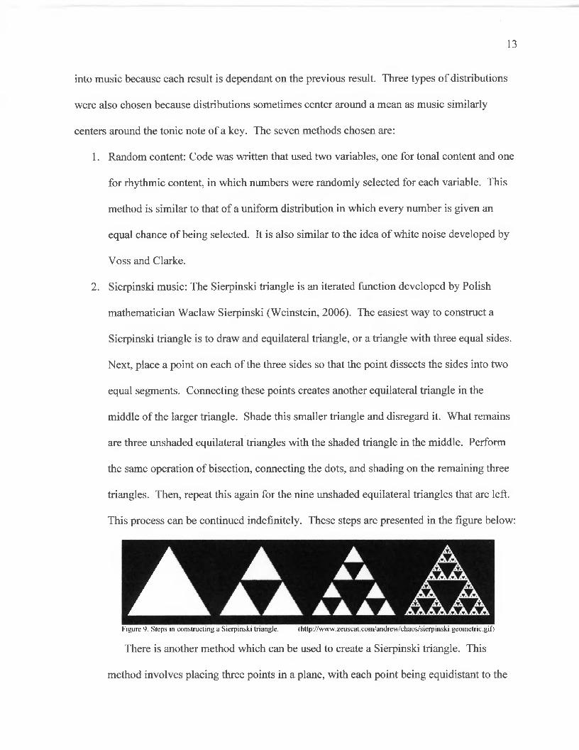
2. Sierpinski music: The Sierpinski triangle is an iterated function developed by Polish

mathematician Waclaw Sierpinski (Weinstein, 2006). The easiest way to construct a

Sierpinski triangle is to draw and equilateral triangle, or a triangle with three equal sides.

Next, place a point on each of the three sides so that the point dissects the sides into two

equal segments. Connecting these points creates another equilateral triangle in the

middle of the larger triangle. Shade this smaller triangle and disregard it. What remains

are three unshaded equilateral triangles with the shaded triangle in the middle. Perform

the same operation of bisection, connecting the dots, and shading on the remaining three

triangles. Then, repeat this again for the nine unshaded equilateral triangles that are left.

This process can be continued indefinitely. These steps are presented in the figure below:

13

Figure 9. Steps in constructing a Sierpinski triangle. (http://www.zeuscat.com/andrew/chaos/sierpinski.geometric.gif)

There is another method which can be used to create a Sierpinski triangle. This

method involves placing three points in a plane, with each point being equidistant to the

14

other two. This creates the skeleton of an equilateral triangle. Then place a random point

such that the point lies inside the space created by the other three points. Pick one of the

three vertices at random and place the next point halfway between this vertex and the

random point. All of the remaining points are found in this fashion, by being placed

halfway between the previous point and one of the vertices. The more points that are

plotted, the closer the picture will resemble a Sierpinski triangle. It takes many hundreds

of thousands of points to get the picture to resemble the Sierpinski triangle. Due to the

time consuming nature of this process, program code has been written that allows the

user to input how many points are desired and then creates the appropriate picture. This

code was modified to give data rather than a picture of a Sierpinski triangle.

3. Chaotic unimodal quadratic maps: Code was written which uses the topological entropy

of the family of quadratic maps that stays within the interval of (0, 1) on the x plane.

This code contains a variable λ which must be in the range of 3.6 < λ < 4.0 to obtain a

chaotic map. The code outputs the x-coordinates of points at each iteration of the

function.

4. Linear distribution: A linear distribution is a distribution in which two variables are

assigned random values, as in a uniform distribution. The lower of these two numbers is

then selected. Code was written in which the data was selected from the lower value in a

series which contained two values.

5. Cauchy distribution: A Cauchy distribution, named after French mathematician Augustin

Cauchy, is a distribution in which a set of values are scaled by a number, a, in

relationship to the mean of the values, which is zero as the nature of a Cauchy

distribution is symmetrical. Code was written which generates Cauchy distributed

variables by using the tangent of a uniformly distributed variable.

6. Fractal music: Many codes have been written that attempt to produce fractal music. The

code used in this project has been adapted from the method described by Richard Voss in

Gardner’s article “White, Brown, and Fractal Music” (1992, pp. 12-14). In this article

Voss suggests using three different dice to simulate fractal music.

7. Random walk: Code was written that creates music that moves in stepwise motion. This

means the notes and durations move to adjacent notes and durations. This type of motion

is similar to Brownian motion and is used to approximate brown noise.

The program Matlab 7.3 (2006) was used for all code writing and program execution in

obtaining the results. All program code used in this project can be found in Appendix A. After

obtaining the data from Matlab 7.3, the numbers were given musical values with each tone or

duration corresponding to each number. The program Finale 2002 (2001) was used to input the

musical content and essentially write the melody. After writing the melody, it was converted to a

midi file, a type of audio file that uses electronic noises to represent the music. Each of the

melodies was analyzed both visually, from the Finale representation, and aurally, from the midi

file. The musical content of each melody was put into a musical category consistent with music

theory and music history standards of Western music. The categories are as follows:

1. Baroque and earlier: This classification implies that the melody displayed the

characteristics of staying in a particular key, used mostly stepwise motion (notes moving to

adjacent pitches), and contained a discemable climax point.

15

2. Classical: This classification implies that the melody displayed the characteristics of

staying mostly in one key with some notes outside the key, contained wider intervals, and

still maintained a discemable climax.

3. Romantic: This classification implies that the melody still showed some signs of having a

key structure, but moved outside of the structure more and more, is more likely to contain

augmented and diminished intervals between notes, while still maintaining a discemable

climax.

4. Impressionist: This classification implies that the melody shows little sign of having a key

structure, but still follows certain rules of tonality. Alternative scales, like the whole tone

scale and the octatonic scale, can often be found. The melody has the characteristic that it

is smooth and sounds dreamlike.

5. 20th Century: This classification implies that the melody does not show any sign of having

a particular key, moves in an erratic motion, and contains no discemable climax point.

In constmcting the melodies for this project, some common constraints have been applied to

them all. The melodies all consist of notes common to the vocal range of a soprano vocalist.

This means that the notes available for each melody range from middle C being the lowest note

and the G a major 12th above middle C the highest note. This provides a range of twenty notes of

the chromatic scale for each melody. This constraint was applied in order to make the melody

possible to be sung by a single vocalist or played by a single instrument. Also the rhythmic

content of the melody was dependent on the mathematical procedure used to obtain the tonal

content. The notes have been confined to six durations: a whole note, a half note, a dotted half

note, a quarter note, a dotted quarter note, and an eighth note. This constraint was applied in

16

17

order to avoid the short durations of a sixteenth note or shorter which would have made it

difficult for the listener to hear the tonal content at the default tempo of the Finale program. The

melodies were also restricted to containing twenty notes. This means that each created melody

had the same number of notes; this does not mean that the melodies are all the same length. The

actual length of the melody depends upon the duration of these notes and is not fixed but lies

between being twenty eighth notes at the shortest and twenty whole notes at the longest. All

notes that are tied together count as one note. The notes are tied because the time signature was

left in common time, which means that there are four beats per measure and the quarter note

receives one beat. For the purposes of this project the time signature does not matter, but due to

the program that was used to input the music, it was necessary to have one, and common time is

the default.

Results

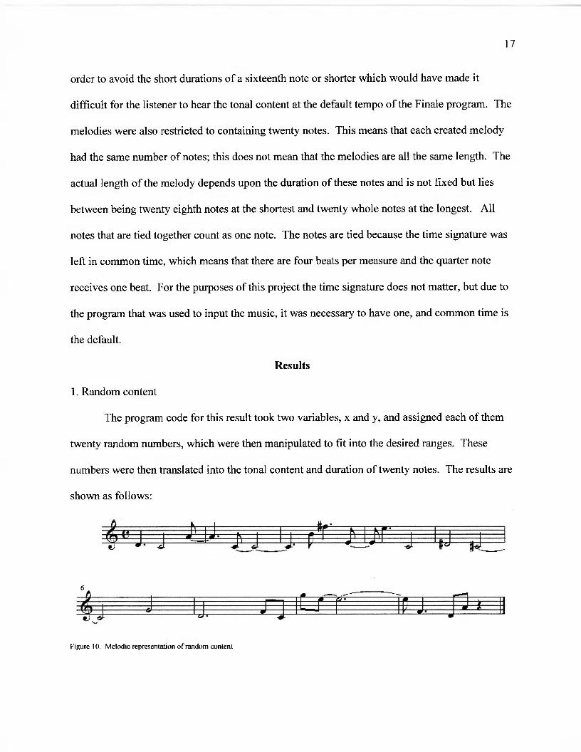
1. Random content

The program code for this result took two variables, x and y, and assigned each of them

twenty random numbers, which were then manipulated to fit into the desired ranges. These

numbers were then translated into the tonal content and duration of twenty notes. The results are

shown as follows:

Figure 10. Melodic representation o f random content

1 8

Musically, the melody is almost impressionistic. The notes do not fall into any one key,

but the note C is repeated several times throughout the melody. Also, there appears to be a

climax note in measure eight, with the G, but it quickly moves to the E, and nothing is resolved.

This melody is certainly twentieth century, which is to be expected as it is a random assortment

of pitches.

2. Sierpinski music

The program code for this result was modified from previous code that was written for a

program that graphs a Sierpinski triangle. Two variables, x and y, were assigned a random

value. A third variable was also picked at random. If this third variable was less than 0.33 then

x and y were divided by two. If the variable was between 0.33 and 0.66 then one was added to x

and then divided by two, while y was simply divided by 2. If the variable did not meet the first

two criteria, then one half was added to x, which was subsequently divided by two, and the

square root of three divided by two was added to y, which was subsequently divided by two.

This operation was performed twenty times for each variable, the numbers were manipulated into

the correct ranges, and the numbers were translated into the tonal content and duration of the

melody. The results are shown as follows:

Figure 11. Melodic representation o f Sierpinski music.

19

This melody has the potential to be classified in a number of ways. The first three notes

could be the outline of a C major chord or an A minor chord. When considering the next four

notes in addition to the first three, the outline of an F-sharp half diminished seventh chord

emerges, which would be found in the key of G-major. The next two notes, B and D, are two of

the tones that make up a G major chord, but without the G this tonality is not established. In the

last five measures, there are two instances where a C is followed by an F-sharp followed by a G-

sharp. The repetition of melodic material is known as a motif. The motif is the basic building

block of most pieces of music. In other words, composers tend to start with motifs and then

expand upon them. Since this comes near the end of the melody, it is an interesting occurrence

but is not likely to be significant especially because it does not fall into the key that was semi-

established in the beginning. Visually and aurally the melody is organized with alternations

between large intervals and small intervals. The exceptions to this occur in measures three, nine,

ten, and fourteen where there are two consecutive small or large intervals. This melody is

impressionist because it nearly establishes a key and contains some organizational content. Also,

the final interval is a minor third. This is consistent with impressionist music, as many

impressionist composers would use mediant cadences, a type of ending that consists of the

chords moving by the interval of a third.

3. Chaotic unimodal quadratic maps

The program code for this result was based on a formula found in Block et al. (1989).

Two variables, x and y, are given a random value. This value is then used in the following

formula: x(i) = lam * x(i -1) * (1 - x(i -1)), where i is an index separating the different values of

x, and lam (lambda) is a variable representing a parameter which affects the height of the map

2 0

(Block et al., 1989, p. 937). A similar formula was used for y. The quadratic maps were found

to be chaotic (non-terminating and non-repeating) for lambda between the values of 3.6 and 4.0.

The interval (0,1) on the x-plane was split into twenty equal pieces and each value of x was

rounded down to the nearest value in the increment. This process was repeated to find the values

of y, except the interval was split into six equal pieces. This put the values of x and y into the

appropriate ranges. The data was then transcribed into the tonal content and duration of the

melody. In order to examine the different melodic output for different values of lambda, three

results were taken with three different values of lambda: 3.8, 3.9, and 4.0. The results are shown

as follows:

Figure 12. Melodic representation o f chaotic unimodal quadratic maps with lambda set at 3.8

Figure 13. Melodic representation o f chaotic unimodal quadratic maps with lambda set at 3 .9

Figure 14. Melodic representation o f chaotic unimodal quadratic maps with lambda set at 4.0

21

The melody that resulted from lambda being set at 3.8 contains some cohesive elements.

Rhythmically the melody has a lot of syncopation, which means that the emphasized notes do not

fall on the beat. Examples of this syncopation can be found in every measure. The tones present

in this melody are consistent with the key of B major or G-sharp minor, except for the D, C, and

F found in the last two measures. The ordering of the notes adds to the tonal feel. The first

measure contains the notes F-sharp, E, and A-sharp, which could potentially outline an F-sharp

dominant seventh (F#7) chord. The next measure contains a D-sharp, B, and F-sharp, which

outlines a B major chord (BM) and adds merit to this melody being in the key of B major. A

similar sequence of tones occurs again immediately following the last F-sharp so that the

majority of the melody seems to be a progression from an F# to BM to F# to BM. The

intervals between the notes are quite large and uncommon for a melody before the twentieth

century, but because of the other characteristics that make this sound tonal and rhythmically

coherent, it is closer to the style of Romanticism.

The melody that resulted from lambda being set at 3.9 is similar to the previous melody

in many respects. Apart from two notes, an F in measure five and a C in measure seven, the

notes of this melody all fit in the key of either D major or B minor. The first note of the melody

is a B, which is usually a strong indication of a melody’s tonality. Rhythmically, this melody is

not as interesting as the melody that precedes it, but it does contain a rhythmic cadence in the

final four notes. This rhythmic cadence consists of three notes of increasingly short duration

followed by a longer note, which gives a sense of finality. A similar pattern of notes occur in

measures seven and eight (E, C, F-sharp, and E, B, F-sharp) which are rhythmically identical.

This creates a semi-motif, giving a sense of cohesion to the ending. The amount of tonal

material and rhythmic similarity place this melody in the Romantic category.

2 2

Where the tonality of the previous two melodies is easy to infer, the tonality of the third

melody achieved from this method is more ambiguous. At first glance the melody appears to be

in the key of B minor because of the F-sharps throughout the passage and the A-sharp in measure

one. The tone C appears in this melody five times which negates the application of this key. A

motif of rhythmically identical occurrences of E, C, and F-sharp occurs three times in the last

four measures of the melody. This motif holds the second half of the melody together. The last

note of the melody, an F-sharp eighth note, leaves the melody sounding unfinished, and is most

likely to leave the listener desiring some kind of resolution. There are also a lot of large intervals

between the notes in this melody. These large intervals and the lack of key place this melody in

the twentieth century category.

These three melodies have quite a bit in common. This is to be expected because all of

the data for the melodies was obtained from the same program. The first two melodies share an

implied tonality and were placed in the same category (Romanticism). The motif that occurs in

the third melody also occurs once in the second melody in measure seven. All three melodies

contain at least three F-sharp eighth notes and some syncopation. While each melody is musical

in a different way, they all contain some of the same characteristics.

4. Linear distribution

The program code written for this result was adapted from code found in Dodge and Jerse

(1985, p. 270). The code written by Dodge and Jerse was written in FORTRAN language, a

coding language that was developed in the 1950s by IBM. This was adapted to fit the language

used in Matlab 7.3. In the code, four variables, x1, x2 , y1, and y2 , were given random values.

The lower value of the two x’s and two y’s were taken, then manipulated into the desired ranges

23

and translated into the musical content. The results are shown as follows:

Figure 15. Melodic representation o f a linear distribution.

The first three measures of the melody contain the first three notes of the A major scale,

which implies that the melody is in the key of A major. The rest of the melody does not follow

this key. In measure four the A moves to a C which sounds like a modulation. A modulation is

when a piece of music moves from one key to another. Modulations are common in music and

usually signify a change in thematic material. This idea is consistent with the rhythms and

intervals of the melody. The first three measures contain longer notes that move by small

intervals while the rest of the melody contains shorter notes and larger intervals. The notes from

measure four to measure nine, starting and ending on C, comprise the first six notes of an

octatonic scale. An octatonic scale is a scale that contains notes that alternate between whole

steps and half steps. A half step is the distance between two adjacent chromatic tones and is the

smallest interval occurring in the common tuning system used in Western music. A whole step

equals two half steps. The notes in measures seven and eight comprise a C minor seventh chord.

A C minor seventh chord consists of C, E-flat, G, and B-flat. The note D-sharp is enharmonic to

E-flat, and similarly the A-sharp is enharmonic to B-flat. When two notes are enharmonic, it

means that the notes have different names but produce the same sound. For the ease of notation,

all notes were written as sharp or natural (neither flat nor sharp). This leaves the possibility for

notes that can function musically as enharmonic notes as they could have easily have been

notated differently. The presence of tonal material and a partial octatonic scale in this melody

categorize it as Impressionist.

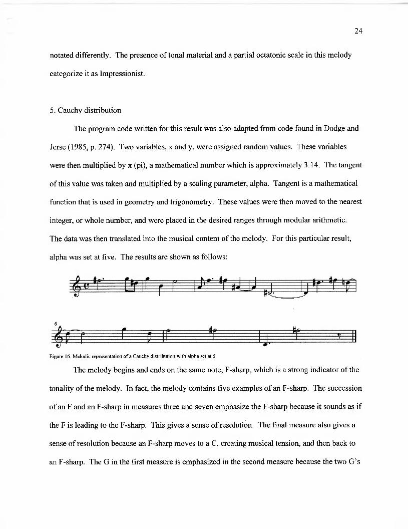
5. Cauchy distribution

The program code written for this result was also adapted from code found in Dodge and

Jerse (1985, p. 274). Two variables, x and y, were assigned random values. These variables

were then multiplied by π (pi), a mathematical number which is approximately 3.14. The tangent

of this value was taken and multiplied by a scaling parameter, alpha. Tangent is a mathematical

function that is used in geometry and trigonometry. These values were then moved to the nearest

integer, or whole number, and were placed in the desired ranges through modular arithmetic.

The data was then translated into the musical content of the melody. For this particular result,

alpha was set at five. The results are shown as follows:

2 4

Figure 16. Melodic representation o f a Cauchy distribution with alpha set at 5.

The melody begins and ends on the same note, F-sharp, which is a strong indicator of the

tonality of the melody. In fact, the melody contains five examples of an F-sharp. The succession

of an F and an F-sharp in measures three and seven emphasize the F-sharp because it sounds as if

the F is leading to the F-sharp. This gives a sense of resolution. The final measure also gives a

sense of resolution because an F-sharp moves to a C, creating musical tension, and then back to

an F-sharp. The G in the first measure is emphasized in the second measure because the two G’s

occur so rapidly in succession. The notes of measure two (G, B, and E) outline an E minor

chord. The notes of measures four and five (A-sharp, D-sharp, and F-sharp) outline a D-sharp

minor chord. These two chords in such close context give the melody a sense of atonality, or a

sense of having no key. This conflicts with the strong sense of F-sharp that is presented in the

first and last notes. This melody falls into the classification of Twentieth Century because it is

atonal despite the fact that it relies heavily on the note of F-sharp and ends with reasonable

resolution.

6. Fractal music

The program code written for this result was adapted from code found in Dodge and Jerse

(1985, p. 290). The code by Dodge and Jerse was based on an algorithm given by Richard Voss,

one of the developers of this concept, in the article “White, Brown, and Fractal Music” by

Gardner (1992, pp. 12-14). This algorithm does not recreate the formula developed by Richard

Voss and John Clarke, but it is a close approximation. Two variables, x and y, were given

random values and put through this algorithm. The values were then rounded down to the

nearest integer and were put in the desired ranges through modular arithmetic. The data was

then translated into musical content. The results are shown as follows:

Figure 17. Melodic representation o f fractal music.

26

At first glance, this melody sticks out because it repeats the same note, a C-sharp, ten

times. It repeats the note at different durations, but the pitch stays the same. Ignoring this

occurrence for a moment, the melody starts with a classic chord progression. The first three

notes (C, F and G), when taken as the roots of a chord, create the I-IV-V progression in the key

of C major. The roman numerals represent the chord built on the scale degree. So since C is the

first note of a C major scale, the C chord is the I chord. Similarly the F is the IV chord and the G

is the V chord. This progression is probably the most used progression in western and popular

music. Most pop songs rely on the I-IV-V progression as the basis of the entire song. A good

example of this is the song “Twist and Shout” written by Phil Medley and Bert Russell (1962),

which uses the C, F, and G major chords. After the I-IV-V progression establishes the melody as

in the key of C major, it moves to a D-sharp and the repeated C-sharp. These notes do not fit in

the key of C major and cannot reasonably be explained. After the C-sharp is repeated several

times, it moves to a C natural, which gives a sense of resolution, because this is the note on

which the melody began. The last four notes of the melody are an alternation between C and D-

sharp. Since the D-sharp enharmonically related to E-flat, this ending implies a C minor chord,

which consists of C, E-flat, and G. This shift seems to indicate that the melody started in the key

of C major and ended in the key of C minor. A modulation between major and minor key of the

same pitch is quite common in music. The beginning and end of this melody represent some of

the basic characteristics of music and, taken alone, would be characterized as Baroque; however

the middle of the melody cannot be ignored as it does not follow these characteristics. This

melody is categorized as Romantic because it contains strong enough tonal material to be

considered tonal, yet it is not consistent enough to be Classical or Baroque.

27

7. Random walk

The program code written for this result was adapted Dodge and Jerse (1985, p. 289).

This program simulates Brownian motion, which was the basis for brown music described by

Richard Voss and John Clarke in their article 1 / f noise’ in music: Music from 1/f noise”

(1978). Two variables, x and y, were assigned random values. A third variable, u, was also

given a random value. If the value of u was less than one half, one was subtracted from the

values of x and y. If the value of u was greater than or equal to one half, one was added to the

values of x and y. The values of x and y were then lowered to the nearest integer and placed in

the desired ranges through modular arithmetic. The data was then translated into musical

content. The results are shown as follows:

Figure 18. Melodic representation o f a random walk.

This is a simple melody that only contains four distinct pitches. These pitches are the

first four pitches of the chromatic scale, a scale which moves by half steps through all of the

twelve distinct musical pitches. Since this melody is a “walk,” the notes are closely related to

one another, and the only motion possible is adjacent motion. Likewise the durations of the

notes are closely related and each pitch has the same duration each time it occurs. This melody

is placed into the category of Impressionist because it uses the chromatic scale and creates a

sound that is characteristic of this style.

28

Discussion and Conclusions

The results that I obtained in this project provided a variety of interesting musical

characteristics. While none of the results could be classified as Baroque or Classical, I was

pleased that some of the melodies contained some characteristics of those musical styles. The

melodies would have contained more of these characteristics if I had put further constraints on

the data. For instance, The data could have manipulated so that it only represented the seven

natural notes which comprise a C major scale (C, D, E, F, G, A, and B). This would have

presented melodies that were more familiar to the ear and possibilities of modal melodies.

Modal melodies are melodies based on modal scales, which are scales that are similar to major

and minor scales but are used less often. I feel that this would have been equally interesting. I

chose to use all chromatic tones within a certain interval because, while I was doing research, all

of the examples I could find of the music made from work of Richard Voss and John Clarke was

made so that the notes all fit into a key. I found these examples in the original article by Voss

and Clarke (1978, pp. 262-3), in the article by Gardner (1992, pp. 16-18), and in an article by

Thomsen (1980, p. 190). I wanted to expand the note choice to see if the methods still gave the

same results. I am pleased that the approximations of white, fractal, and brown music still

followed the same general trend as the examples I found. The completely random notes (white

noise) were erratic; the music based on the walk (brown noise) was highly correlated; and the

fractal music was somewhere in between, although not as musical as the examples I had found.

The other melodies that were not based on the ideas of Voss and Clarke also turned out

nicely. When I first obtained my data and translated it into music, I was a little disappointed

because at first glance it all looked the same. Once I started analyzing the melodies further, I got

very excited over anything that could be explained musically. I think that the melodies that I

found not only illustrate how mathematics can be used to create something artistic but also that

music cannot be made by logic and mathematics alone. Music must have some structure but also

some creative input that comes from the mind of a composer.

If I had more time to work with these ideas, I would pursue almost every aspect of the

research further. First, I would like to explore more methods in creating these melodies. I felt

that the work of Iannis Xenakis was interesting and would have liked to use it as one of my

methods, but his explanations of his methods were beyond my understanding. Perhaps if I had

more time, I could penetrate their meanings and find a way to make them work. I would also

like to try more mathematical distributions. I relied heavily on the book Computer Music by

Charles Dodge and Thomas A. Jerse (1985) for a start in writing the code for my programs, and

they had several more distributions that I did not attempt. I would also like to re-examine the

Cauchy distribution and see what my results would be depending on how I altered the parameter

alpha.

In addition to broadening the mathematical concepts used, I would also like to broaden

the musical range of my results. I chose a range of twenty chromatic tones so that the notes

would not be too far from one another and would have some chance of relating to one another. If

I had more time I would expand the range to all eighty-eight tones possible on the standard piano

keyboard. I feel that this would alter my results but hopefully not too drastically. Similarly I

would expand the number of note durations I used. I only used six different note durations, and,

at times, I felt this was too few. I did not, however, want to use durations that would be so short

that there was a chance my melody would pass by too quickly and the tonal content would be

impossible to distinguish and analyze aurally.

29

I would also like to expand the length of my melodies. I picked the melodies to be

twenty notes in length because I felt that this length was long enough to get an idea of what kind

of music the mathematical concept produced yet short enough to be able to work with easily.

Ideally the melodies would be much longer, even as long as one hundred notes. I also think that

it would be interesting and valuable to attempt to harmonize these melodies. The process of

harmonization is where notes are added underneath the melody in order to support it and give it

direction. I mentioned several times in the paper how some notes outlined a chord or could

represent a chord. In harmonizing the melody this chord would be added underneath the melody,

and the two would play simultaneously. In the early stages of this project I considered

harmonizing the melodies that I constructed, but this process is lengthy, time consuming, and

most of the time frustrating due to the number of rules in music theory that must be followed.

31

Bibliography

Benward, B. & Saker, M. (2003). Music in Theory and Practice 7th Edition, Volume 1. Boston: McGraw Hill.

Block, L., Keesling, J., Li, S., & Peterson, K. (1989, June). An Improved Algorithm for Computing Topological Entropy. Journal o f Statistical Physics, 55, 929-939.

Cross, J. (2004). Composing with numbers: sets, rows and magic squares. In J. Fauvel,R. Flood, & R. Wilson (Eds.) Music and Mathematics: From Pythagoras to Fractals. New York: Oxford University Press.

Dodge, C., & Jerse, T. (1985). Computer Music: Synthesis, Composition, and Performance. New York: Schirmer Books.

Finale 2002. (2001). Finale. (Version 2002.rl). [Computer Software]. Eden Prairie, MN: Coda Music Technology.

Gamer, C., & Wilson, R. (2004). Microtones and projective planes. . In J. Fauvel,R. Flood, & R. Wilson (Eds.) Music and Mathematics: From Pythagoras to Fractals. New York: Oxford University Press.

Gardner, M. (1992). White, Brown, and Fractal Music. In M. Gardner (Ed.) Fractal Music, HyperCards and more: Mathematical Recreations from Scientific American Magazine. New York: W.H. Freeman and Company.

Harkleroad, L. (2006). The Math Behind the Music. New York: Cambridge University Press.

Ho, A. (1995). Sierpinski Triangle. Chaos Homepage. Available [On-Line]: http://www. zeuscat.com/ andrew/ chaos/ sierpinski .html.

Johnson, R. (2004). Composing with fractals. In J. Fauvel, R. Flood, & R. Wilson(Eds.) Music and Mathematics: From Pythagoras to Fractals. New York: Oxford University Press.

Mandelbrot, B. (1983). The Fractal Geometry o f Nature. New York: W. H. Freeman and Company.

Mandelbrot Set. (2007). Wikipedia. Available [On-Line]: http://en.wikipedia.org/wiki/ Mandelbrot set.

Matlab7.3. (2006) Matlab (Version 7.3.0.267[R2006b]). [Computer Software]. Natick, MA: The Mathworks Inc.

Medley, P., & Russell, B. (1962). Twist and Shout. [Recorded by The Beatles]. On Introducing... The Beatles [LP]. London: Tollie Records (1964).

Schroeder M. (1991). Fractals, Chaos, and Power Laws: Minutes from an Infinite Paradise. New York: W. H. Freeman and Company.

Thomsen, D. (1980, March 22). Making Music Fractally. Science News, 117, 187-190.

Voss, R. & Clarke, J. (1978, January), noise” in music: Music form ̂ noise. The

Journal o f the Acoustical Society o f America, 63( 1), 258-263.

Weinstein, E. (2006) Sierpinski Sieve. Wolfram Mathworld. Available [On-Line]: http://mathworld.wolfram.com/SierpinskiSieve.html.

Xenakis, I. (1972). Formalized Music: Thought and Mathematics in Composition. Bloomington, Indiana: Indiana University Press.

Appendix A

Program Code

Below is the code that was written for this project. The code for this project was written

in Matlab 7.3 by Dr. Kevin Peterson and myself. Much of the code was adapted from the book

Computer Music by Charles Dodge and Thomas A. Jerse (1985)

1. Random content:

%random number generator where n is the number of iterations

function tt=calc (n)

x(l)= rand

y (1)=rand

for i=l:n

x (i)=rand

y (i)=rand

end

x=floor(20*x)+1;

y=floor(6*y)+1;

x, y

33

2. Sierpinski music:

name this sierpmusic.m it is run by typing sierpmusic(n) where

n is the number of iterations,

function tt-calc(n)

x=rand;

34

y=rand;

for i=0:n

pick=rand;

if pick<.33,

nx=x/2;

ny=y/2;

elseif pick<.66,

nx=(x+1)/2;

ny—y/2;

else

nx=(x+(1/2))/2;

ny=(y+(sqrt(3)/2))/2;

end

x=nx;

y=ny;

note(i+1)=floor(20*x)+1;

rhythm(i+1)=floor(6*y)+1;

end

note

rhythm

3. Chaotic unimodal quadratic maps

name this unimod.m it is run by typing unimod(n) where

n is the number of iterations.

function tt=calc(n,lam)

35

x (1)=rand;

y (1)=rand;

for i=2:n

x (i)=lam*x(i-1)*(l-x(i-l));

y (i)=lam*x(i-1)* (l-x(i-l));

end

x=floor(20*x)+1;

y=floor(6*y) +1;

x, y

4. Linear distribution

name this linear.m to run type linear(n) where n is the number of

iterations

function tt=calc(n)

for i=l:n

xl(i) = rand;

x2(i) = rand;

yl (i) = rand;

y2(i) = rand;

if x2 < xl;

xl = x2;

end

if y2 < yl;

yl = y2;

end

36

end

xl=floor(20*xl)+1;

yl=floor(6*y2)+1;

xl, yl

5. Cauchy distribution

name this cauchy.m it is run by typing cauchy (n, alpha) where n

is the number of results desired and alpha is scaling parameter

function tt=calc(n,alpha)

for i=l:n

x(i) = rand;

y(i) = rand;

u = x*pi;

v = y*pi;

notes = alpha*tan(u);

rhythm = alpha*tan(v);

end

notes = floor (notes);

rhythm = floor (rhythm);

notes = mod(notes,20);

rhythm = mod(rhythm,6);

notes, rhythm

37

6. Fractal music:

name this fractal.m it is run by typing fractal(n,m) where

n is the number of possible values and m is the number of iterations

function tt=calc(n,m)

x(l)= rand;

y(l)= rand;

for i=2:m;

k = n / 2;

r = 1/n;

while k >= 1;

j = k/x(i—1);

if j == 1;

x(i-l)= x(i-l) - k;

end

u=rand;

if u < r;

j= i-j;

end

x ( i ) =0;

x (i) = x (i) + j *k;

k=k/2;

r=r*2;

end

end

for i=2:m;

38

k = n / 2 ;

r = 1/n;

while k >= 1;

j=k/y(i—1);

if j==l;

y(i—1)= y(i-l) - k;

end

u=rand;

if u < r;

j= l-j;

end

y (i) = 0 ;

y (i) = y(i) + j*k;

k=k/2;

r=r * 2;

end

end

x=floor(x);

y=floor(y);

x=mod(x,20);

y=mod(y,6);

x,y

39

7. Random walk

name this walk.m it is run by typing walk(n) where n is the number

of iterations.

function tt=calc(n)

x(l) = rand;

y(l) = rand;

for i=2:n

h=l;

u=rand;

if u < .5;

h=-l;

end

x(i) = x(i-l) + h;

y (i) = y(i-l) + h;

end

x=floor(x);

y=floor(y) ;

x=mod(x,20) ;

y=mod(y,6);

x,y

4 0

Appendix B

Data

Below is the actual data that I obtained after running each of the programs with the code

written above. In the cases where x and y were used as final variables, x represents the numbers

used for pitch, and y represents the numbers used for duration of the pitch.

1. Random content:

X = 3 13 10 1 12 19 5 17 1 4 2 8

3 6 1 20 17 6 3 10

y = 5 2 2 1 6 5 4 5 2 2 1 2

3 6 6 6 1 5 6 6

2. Sierpinski music:

note = 5 13 17 19 10 10 5 3 12 11 6 13

7 9 15 13 7 9 5 8 9

rhythm = 3 2 1 1 1 3 2 1 1 3 2 1

1 3 2 4 2 4 2 4 5

3. Chaotic unimodal quadratic maps:

Lambda = 3.8

x — 7 17 11 19 4 12 19 5 14 17 11 19

4 12 19 5 15 16 13 18

41

y = 2 6 4 6 2 4 6 2 5 6 4 6

2 4 6 2 5 5 4 6

Lambda = 3.9

x = 12 20 3 10 20 2 7 18 8 19 5 15

17 13 19 6 17 12 19 4

y = 5 6 1 3 6 1 3 6 3 6 2 5

5 4 6 2 5 4 6 2

Lambda = 4

x = 7 17 11 20 1 1 2 6 17 13 19 6

17 13 19 5 15 17 13 19

y = 5 6 4 6 1 1 1 2 5 4 6 2

5 4 6 2 5 5 4 6

4. Linear distribution:

x 1 = 10 12 14 12 9 13 5 2 17 5 16 7

20 16 8 13 11 3 13 5

yl - 1 2 3 2 2 3 3 5 4 5 3 5

2 2 5 2 4 4 3 5

4 2

5. Cauchy distribution:

notes = 18 9 15 19 11 16 9 17 18 10 3 15

18 14 19 14 17 18 0 18

rhythm = 2 5 5 3 3 1 5 4 3 1 0 4

3 2 3 5 2 2 4 1

6. Fractal music:

x = 0 5 19 5 19 15 1 1 1 1 1 1

1 1 1 1 0 15 0 15

y - 0 4 0 5 3 5 4 0 1 0 5 3

5 4 0 5 3 5 4 0

7. Random walk:

oIIX 1 2 3 2 1 2 3 2 1 2 3

2 1 2 1 2 1 2 3

y = 0 1 2 3 2 1 2 3 2 1 2 3

2 1 2 1 2 1 2 3

Appendix C

Conversion Charts:

Below are some charts that explain how the numbers obtained in the data were translated

into the musical content. The symbol # implies sharp (C# means C-sharp). The numbers in the

row labeled Case 1 were used for methods 1-4. The numbers in the rows labeled Case 2 were

used for methods 5-7.

43

Pitches:

C C# D D# E F F# G G# A A# B C C# D D# E F F# GCase 1: 1 2 3 4 5 6 7 8 9 10 11 12 13 14 15 16 17 18 19 20Case 2: 0 1 2 3 4 5 6 7 8 9 10 11 12 13 14 15 16 17 18 19

Duiation:

Case 1: 1 2 3 4 5 6Case 2: 0 1 2 3 4 5

Companion CD

As this project contained music that is intended to be examined aurally as well as

visually, I deemed it appropriate to provide a CD that contained the melodies on it. The files on

this CD are MIDI files, and must be opened on a computer and played in a media player that

supports MIDI files. I have a few suggestions in listening to this CD. The first suggestion is to

look at the notated music contained in this paper while listening to the melody. It will be easier

to make sense of what you hear if you can see it. The second suggestion would be not to try to

listen to all of the melodies at once. When listening to them in immediate succession, it is easy

to get the melodies confused and soon they may all sound the same. This is why I suggest

tackling them one at a time. The file list is indicated below:

Random.mid: Melodic representation of random content

Sierpinski.mid: Melodic representation of Sierpinski music

Unimod38.mid: Melodic representation of chaotic unimodal quadratic maps with lambda set to

3.8

Unimod39.mid: Melodic representation of chaotic unimodal quadratic maps with lambda set to

3.9

Unimod4.mid: Melodic representation of chaotic unimodal quadratic maps with lambda set to 4

Linear.mid: Melodic representation of linear distribution

Cauchy .mid: Melodic representation of Cauchy distribution

Fractal.mid: Melodic representation of fractal music

Walk.mid: Melodic representation of random walk

4 4

A p p e n d ix D