Mathematical formulation and analysis of the nonlinear system reconstruction of the online image-guided adaptive control of hyperthermia

Page 1

Mathematical formulation and analysis of the nonlinear systemreconstruction of the online image-guided adaptive controlof hyperthermia

Kung-Shan Cheng,a� Mark W. Dewhirst, Paul F. Stauffer, and Shiva DasDivision of Radiation Oncology, Duke University Medical Center, Box 3295, Durham,North Carolina 27710

�Received 15 April 2009; revised 21 December 2009; accepted for publication 23 December 2009;published 5 February 2010�

Purpose: A nonlinear system reconstruction can theoretically provide timely system reconstructionwhen designing a real-time image-guided adaptive control for multisource heating for hyperther-mia. This clinical need motivates an analysis of the essential mathematical characteristics andconstraints of such an approach.Methods: The implicit function theorem �IFT�, the Karush–Kuhn–Tucker �KKT� necessary condi-tion of optimality, and the Tikhonov–Phillips regularization �TPR� were used to analyze and deter-mine the requirements of the optimal system reconstruction. Two mutually exclusive generic ap-proaches were analyzed to reconstruct the physical system: The traditional full reconstruction andthe recently suggested partial reconstruction. Rigorous mathematical analysis based on IFT, KKT,and TPR was provided for all four possible nonlinear reconstructions: �1� Nonlinear noiseless fullreconstruction, �2� nonlinear noisy full reconstruction, �3� nonlinear noiseless partial reconstruction,and �4� nonlinear noisy partial reconstruction, when a class of nonlinear formulations of systemreconstruction is employed.Results: Effective numerical algorithms for solving each of the aforementioned four nonlinearreconstructions were introduced and formal derivations and analyses were provided. The analysesrevealed the necessity of adding regularization when partial reconstruction is used. Regularizationprovides the theoretical support for one to uniquely reconstruct the optimal system. It also helpsalleviate the negative influences of unavoidable measurement noise. Both theoretical analysis andnumerical examples showed the importance of having a good initial guess for accomplishing non-linear system reconstruction.Conclusions: Regularization is mandatory for partial reconstruction to make it well posed. TheTikhonov–Phillips regularized Gauss–Newton algorithm has nice theoretical performance for par-tial reconstruction of systems with and without noise. The Levenberg–Marquardt algorithm is amore robust algorithmic option compared to the Gauss–Newton algorithm for nonlinear full recon-struction. A severe limitation of nonlinear reconstruction is the time consuming calculations re-quired for the derivatives of temperatures to unknowns. Developing a method of model reduction orimplementing a parallel algorithm can resolve this. The results provided herein are applicable tohyperthermia with blood perfusion nonlinearly depending on temperature and in the presence ofthermally significant blood vessels. © 2010 American Association of Physicists in Medicine.�DOI: 10.1118/1.3298005�

Key words: implicit function theorem, Karush–Kuhn–Tucker necessary condition of optimality,optimization, regularization, Gauss–Newton algorithm, Levenberg–Marquardt algorithm, fullreconstruction, and partial reconstruction

I. BACKGROUND AND SIGNIFICANCES

Hyperthermia is a cancer treatment modality that has beenshown clinically capable of enhancing the therapeutic effectsof radiation1 and/or chemotherapy2 because of the elevatedtemperature it induces. Hyperthermia has received increasingattention partially because of the rapid development in medi-cal imaging techniques. This imaging allows clinicians toobtain faster and more detailed patient information to adjustpower focusing.3–5 Consequently, tumor temperature local-ization is improved.

Selective heating is essential to the success of hyperther-

980 Med. Phys. 37 „3…, March 2010 0094-2405/2010/37„3

mia therapy. Only then can the tumor be maximally de-stroyed by spatially confined power, while the surroundingnormal tissues are maximally preserved. The integrated en-vironment of patient and heat sources is hereby referred to asthe system. It is derived from physical laws and can begradually updated by using feedback from a learning pro-cess. To realize accurate confined tumor heating, an accuratemathematical description of the system is essential. The ac-curacy of the system description can be degraded by manyfactors. For example, the tissue electric and thermal proper-ties are usually very patient specific,6,7 and thus there would

be discrepancies between the published values and the actual

980…/980/15/$30.00 © 2010 Am. Assoc. Phys. Med.

Page 2

981 Cheng et al.: Mathematical formulation and analysis of nonlinear system reconstruction 981

values of the patient under treatment. In addition, blood per-fusion that may affect the therapeutic results8,9 can differeven for the same patient from one treatment session to an-other. As such, accurate patient positioning within a flexiblewater bolus is also difficult to be estimated before thetreatment.10 All of these uncertainties and the unavoidablenoise involved in temperature feedback from a medical im-aging scanner, e.g., magnetic resonance imaging �MRI� scan-ner, degrade the reliability of the description of a system.8,9,11

It is clear that the success of hyperthermia therapy requiresadaptation of a system control strategy that provides the mostaccurate dynamic patient-specific information.

The inclusion of a learning strategy distinguishes adaptivecontrol from other control methodologies. Adaptive controlof hyperthermia consists of a learning process and a feed-back kernel. By using a measurement feedback, the learningprocess gradually improves the accuracy of the mathematicalform that describes the system. The feedback kernel appliesthe control rules to steer the power spatially and optimallyand to restrict the power within the tumor.8,11,12 This feed-back kernel also adjusts the total power output to reach andmaintain the desired temperature.13,8

Different formulations of a system require different learn-ing strategies. Although the measuring device and the inte-grated environment of a patient and heat sources involvedremain the same, different computational complexities areassociated with different learning strategies. This is becausedifferent system formulations have different number of inde-pendent variables and different mathematical structures toconvert the same feedback information to corresponding out-put. The number of independent heat sources �M� plays animportant role in estimating the workload of a learning strat-egy. To fully reconstruct the system when M independentheat sources are employed, a linear learning strategy8 theo-retically requires M2 learning steps because its system is anM-by-M Hermitian matrix.14 In contrast, a nonlinear learningstrategy15 requires 6�M steps because its system consists of a3-by-M complex matrix; the number 3 comes from the three-dimensional geometry, M is the number of independent heatsources, and each source has a complex variable that has tworeal components �3�M�2=6�M�. As more heat sources �forexample, M �6� are applied to provide better spatial tem-perature focusing, a nonlinear learning strategy clearly be-comes even more attractive than a linear strategy because itdemands fewer learning steps thus shortens the time expen-diture for learning. However, even when a nonlinear learningstrategy is applied, it could still take long time for a completelearning process. For instance, when a patient is treated by amodern phased-array applicator like BSD-2000 Sigma-Eyeheating applicator �Sigma-Eye/MR, BSD Corporation, SaltLake City, UT� which has 12-paired antennas in three rings,it could take hours for the nonlinear learning process becauseit demands 72 steps of learning correction.15 To further ac-celerate this learning process, a recent research direction is toexplore the development of a learning strategy that only re-quires partial reconstruction. In particular, this strategy at-

tempts to determine the optimal configuration of heat sources

Medical Physics, Vol. 37, No. 3, March 2010

when delivering a spatially confined tumor heating beforethe system is fully reconstructed. Currently, partial recon-struction is addressed in the following published works,8,15

and some approaches incorporating model reduction weredeveloped recently.11,12

There are certain theoretical limitations regarding the de-velopment of a successful partial reconstruction approach us-ing a nonlinear learning strategy, but there is no formal the-oretical analysis highlighting and addressing them.Therefore, the authors were motivated to analyze and empha-size those theoretical considerations and provide solutions toaddress these issues. This paper will describe and analyzealgorithms for nonlinear full and partial reconstructions us-ing feedback with unavoidable noise. Rigorous theoreticalsupport will also be provided for these algorithms. Problemformulation and mathematical analysis will be conducted forproblems with increasing theoretical complexity: From theproblem of nonlinear full reconstruction using noiselessfeedbacks to nonlinear partial reconstruction using noisyfeedbacks. After completing the formulation and analysis forhyperthermia described by linear physical model with con-stant parameters, the analysis will be conducted for morepractical and complicated conditions of hyperthermia withblood perfusion nonlinearly varying with temperature.Lastly, numerical exhibitions will be given, followed bycomparisons between nonlinear and linear formulations ofsystem reconstruction.

II. METHODS FOR THEORETICAL ANALYSIS ANDNUMERICAL EXHIBITION

Theoretical descriptions of the physical processes relatedto the design for real-time image-guided control of hyper-thermia are first provided. Then followed are mathematicaltheorems and the related numerical setups for the purpose ofillustrations.

II.A. Governing equations for the thermal and wavephysics

Using a set of externally applied nonionizing heatsources, the internal temperature of human body is locallyelevated to a therapeutic level and is maintained for a treat-ment period to deliver a lethal thermal dose to the targetcancerous cells. This kind of treatment is called multisourceloco regional hyperthermia. Assuming that the bioheat trans-fer �BHT� process inside human body is linear, the tempera-ture response to a given power deposition is written below,8

T�t,r�� = ��=0

t �V�

G�t − �,r� − r��� · Psum��,r��� · dV� · d� .

�2.1�

Here, the scalar t is time, and the vector r is a function of thex, y, and z variables indicating the spatial position. The func-tion G is called Green’s function,16–19 and Psum denotes the

power deposition delivered by a set of nonionizing sources.

Page 3

982 Cheng et al.: Mathematical formulation and analysis of nonlinear system reconstruction 982

Zero initial and boundary conditions are assumed here tosimplify further analysis. The Green’s function is a compactexpression representing the response of a linear system to animpulsive input. The Green’s function exists regardless ofwhether the linear problem formulation is time invariant orvarying,16 and whether the domain of the problem is finite orinfinite, regular or irregular.17–19 The Green’s function hereimplicitly includes the effects of thermal properties of thepatient and the position of the tumor relative to the patientand the applicator, etc.

There are two types of commonly employed nonionizingsources: Electromagnetic �EM� waves and ultrasonic �US�waves. Richer technical issues are contained in the casewhen EM sources are used than when US sources are used.Therefore, the analysis is based on the use of EM sources;the analysis can be easily reduced to the case when USsources are used.

Assuming wave propagation inside the human body isalso linear by neglecting the cross-talking and mutual cou-pling between sources,20 the resultant power deposition is afunction of the product of the conjugate of the synthesizedelectric field �E field� with itself,

Psum�t,r�� =�

2· E� sum

H · E� sum, r� = �x,y,z� . �2.2�

Here, the superscript H denotes the complex conjugate trans-pose, and � is the electric conductivity.

Based on linearity assumption of the wave propagation,the resultant E field is given by the following equation:

E� sum,3�1�t,r�� = �m=1

M

E� m,3�1 · um = E3�M�t,r�� · u�M�1�t� .

�2.3�

Here, M is the number of antennas, the vector Em denotes theE field from antenna m, and um refers to the mth �complex�antenna configuration.

A controller is required for hyperthermia to generate apower deposition that selectively elevates tumor temperatureand to avoid undesired hot spots in normal tissues, whichwould cause damage, patient pain, or discomfort. Given be-low are theories related to the design for the control of hy-perthermia.

II.B. The design for control of BHT process

It is desirable to obtain a formulation explicitly linkingtogether the clinical outputs �temperatures� and the controlvariables �the driving vector of the heating sources�. For sim-plicity, the derivation assumes that power does not changecontinuously in time. Therefore, the equations in Sec. II Aare simplified and combined to provide one such equation

below,

Medical Physics, Vol. 37, No. 3, March 2010

T�t,r�� = u�H · ��

2· �

�=0

t �V�

G�t − �,r� − r���

· �EM�3H · E3�M�r���� · dV� · d�� · u� . �2.4�

The terms in the parentheses together represent the system,the vector u denotes the driving vector to the heat sources,and T is the output temperature. With this equation, one canproceed to design a controller that adjusts the components ofthe driving vector so that the corresponding temperature re-sponse satisfies the goal of hyperthermia.

A complicated mathematical model more accurately de-scribes the underlying physics. However, a simpler modelbetter serves the purpose of numerically demonstrating theessential theoretical characteristics of the design for a non-linear learning strategy associated with online image-guidedcontrol of hyperthermia. Therefore, a simpler model approxi-mately describing the clinical physics involved is also givenhere,

� · Ct ·dT

dt= − wb · Cb · T +

�

2· u�H · �EM�3

H · E3�M� · u�

⇒dT

dt= − � · T +

�

2 · � · Ct· u�H · �EM�3

H · E3�M� · u�

⇒T�t,r�� = T�0,r�� · exp�− � · t� +�

2 · � · � · Ct· u�H

· �EM�3H · E3�M� · u� · �1 − exp�− � · t�� . �2.5�

Here, � is tissue density, Ct is the specific heat of tissue, wb

indicates the Pennes perfusion,21 � is the effective perfusionfrequency,22 and Cb refers to the specific heat of blood. Theeffective perfusion frequency approximately describes the in-tegrated local cooling from the Pennes blood perfusion21 andthermal conduction at a point inside the patient underwenthyperthermia.23 Hence, the important physical cooling fac-tors known to have significant impacts on hyperthermia24 arepreserved.

II.B.1. The basic ideas of nonlinear learningstrategy

The goal of a learning strategy is to optimally reconstructthe system. Therefore, in this case, the temperature �e.g.,from image feedback� and the driving vector in Eq. �2.1� aregiven information, and the goal is to determine the ensembleof the E fields. The unknowns involved in the ensemble ofthe E fields are identified from the information retrieved. InSec. III the essential features of nonlinear system reconstruc-tion will be analyzed.

There are some essential theorems involved in optimalreconstruction of the system. First described below is theimplicit function theorem �IFT�.25,26 It provides the sufficientconditions required to ensure the existence of a unique solu-tion to a nonlinear reconstruction. Then the Karush–Kuhn–

27

Tucker �KKT� necessary condition of optimality is intro-

Page 4

983 Cheng et al.: Mathematical formulation and analysis of nonlinear system reconstruction 983

duced to provide the necessary condition employed todetermine the optimal solution for a given optimization prob-lem.

II.C. The IFT

IFT is a tool that allows relations to be converted to func-tions. The theorem states that if the equation R�x ,y�=0 �animplicit function� satisfies some mild conditions on its partialderivatives, then, in principle, one can solve this equation fory, at least over some small interval. Geometrically, the locusdefined by R�x ,y�=0 will overlap locally with the graph ofan explicit function y= f�x�.

The theorem is described below using a simple case in-volving only a few variables and parameters; however, it canbe extended to cases involving more variables and or param-eters.

Let f� :R3→R2 be a continuous differentiable �vector-valued� function in two dimensions. Assuming there is apoint �xa ,yb,1 ,yb,2� that satisfies a unique �vector� relationg :R→R2 in two dimensions that works around the neighbor-

�

noise.

Medical Physics, Vol. 37, No. 3, March 2010

hood of this point �xa ,yb,1 ,yb,2� as long as the Jacobian isnonsingular at this point. This function g relates the variablesx, y1, and y2 as yb,1=g1�x� and yb,2=g2�x�. The Jacobian isgiven below,

J�xa,yb,1,yb,2� = � f1

�y1�xa,yb,1,yb,2�

� f1

�y2�xa,yb,1,yb,2�

� f2

�y1�xa,yb,1,yb,2�

� f2

�y2�xa,yb,1,yb,2� .

�2.6�

As shown in the examples below, IFT provides sufficientconditions that ensure the existence of the unique reconstruc-tion regardless the formulation is linear or nonlinear.

II.C.1. Example II.C.1

A famous example in multivariable calculus is given hereto show the power of IFT. This is a two-dimensional coordi-nate transformation between the Cartesian coordinates �x ,y�and the polar coordinates �r ,��.

� f1 = x − r cos � = 0

f2 = y − r sin � = 0� ⇒ J =

� f1

�r

� f1

��

� f2

�r

� f2

�� = − cos � r sin �

− sin � − r cos �� ⇒ det�J� = r . �2.7�

The IFT requires the Jacobian to be nonsingular, i.e., itsdeterminant is nonzero. According to Eq. �2.7�, thisdemands the value r to be nonzero. When this is the case,there is a unique coordinate transformation betweenthe Cartesian coordinates �x ,y� and the polar coordinates�r ,��. However, when r=0, which means IFT isviolated, and then there is no such coordinates transforma-tion.

Rewriting the IFT less formally in nontechnical terms forthe current hyperthermia issue of multisource heating appli-cator system reconstruction, it states that when there are Munknowns, one must have M different equations that satisfycertain conditions imposed by Eq. �2.6� so that a unique fullreconstruction can be ensured.

However, using the IFT alone is insufficient to handle thepractical situations in the presence of unavoidable noise.Since the goal of this paper is to analyze and design a systemreconstruction algorithm to expedite the learning process, to-gether it leads to the employment of the theorem regarding tothe numerical optimization. Next, the KKT necessary condi-tion of optimality is introduced. Based on this condition, onecan better analyze and design a full or a partial reconstruc-tion algorithm to expedite the learning process for the real-time adaptive control of hyperthermia involving unavoidable

II.D. The Karush–Kuhn–Tucker „KKT… necessarycondition of optimality

The KKT conditions are necessary for a solution in non-linear programming to be optimal, provided some regularityconditions are satisfied. This condition is written below.Given an unconstrained quadratic optimization problem, theoptimal solution is a critical point of the objective functionand hence its gradient equals to zero,

minx�M�1

g�x�M�1� = minx�M�1

12 · �f�N�1�x�M�1��2

2. �2.8�

Here, the real scalar function g, which is the half of thesquare of the Euclidean norm of the vector function of f , iscalled the objective function, goal function, or criterion func-tion. The vector function of f has N different components.Each component of the vector function f denotes the differ-ence between the measured and the predicted outputs from agiven excitation. In hyperthermia, this output can be a vectorin which each of its elements is a product of a selectedweighting coefficient and temperature at a point of interest.9

The points of interest could be tumor points only8,9 or in-clude the points in critical normal tissues.13,15 The KKT nec-essary condition indicates that the optimal solution satisfies

the following conditions:

Page 5

984 Cheng et al.: Mathematical formulation and analysis of nonlinear system reconstruction 984

�g

�x�M�1= 0�M�1 = JA�f�N�1,x�1�M

A � · f�N�1�x�M�1� . �2.9�

The superscript A denotes complex conjugate transpose forcomplex variable and transpose for real variable. The firstterm �J� in the right side of the equality is called the Jaco-bian, which denotes the gradient of a vector function.

II.E. Configurations for numerical simulations

It is difficult to understand all the properties of the modelspurely based on the aforementioned advanced mathematicaltheorems. Thus, commercial software MATLAB™ �The Math-Works, Inc., Natick, MA� was used to conduct numericalexperiments to explicitly illustrate the results analyzed usingthe abstract theorems.

The approximate physical model expressed by Eq. �2.5�was used for the aforementioned purpose, but zero initialtemperature was assumed for simplicity. It was also assumedthat there are only three point sources. The target of heatingwas the coordinate origin, and the coordinates of the threesources were �11.5, 0, 0�, �0, �11.5, 0�, and ��11.5, 0, 0�;the unit of the coordinates was centimeter. Note the dimen-sions of this simulation configuration were used to mimic adesign of 10-antenna cylindrical applicator for hyperthermictreatment of extremities that was used in previous studies.9,12

The heating period was 5 min for each single power excita-tion that was used to produce temperature feedback. Thermalinteractions between different excitations were assumed tobe negligible to simplify the analysis. The electric and ther-mal property values28,29,7,30,31 involved for the numericaldemonstrations were given as those for �human� musclewhen the driving frequency of the EM wave was 150 MHz.The electric permittivity was 5.507 188�10−10 F /m, theelectrical conductivity was 0.727 S/m, the permeability was4��10−7 H /m, the density was 1050 kg /m3, the specificheat of muscle was 3639 J/kg K, the specific heat for bloodwas 3770 J/kg K, and the blood perfusion was 3.6 kg /m3 s.

III. ANALYZED RESULTS AND DISCUSSION

In the following sections, effective algorithms and limita-tions for four different types of nonlinear reconstruction areanalyzed, including the combinations of full and partial re-constructions, and noiseless and noisy situations. Then dis-cussions and comparisons with a previously publishedalgorithm15 are given, followed by an analysis for nonlinearsystem reconstruction of adaptive control of hyperthermiawhen the perfusion is nonlinearly temperature dependent.Numerical exhibitions are also presented. Then, comparisonsbetween nonlinear and linear reconstructions are provided.

III.A. Nonlinear noiseless full reconstruction„NNLFR…

A full reconstruction in the absence of noise is first dem-onstrated using a numerical optimization. The optimization

problem is formulated as in Eq. �2.8�. Based on the KKT

Medical Physics, Vol. 37, No. 3, March 2010

necessary optimality condition given in Eq. �2.9�, the optimalsystem reconstructed can be determined by the followingimplicit equations:

0�6·M�1 = h�6·M�1 � JA�f�6·M�1,x�1�6·MA � · f�6·M�1�x�6·M�1� .

�3.1�

Unfortunately, Eq. �3.1� is also a system of nonlinearequations. Since generally there is no closed-form solution toa nonlinear problem, among many algorithms, the Gauss–Newton �GN� algorithm32,33 is chosen to solve Eq. �3.1�.This method is well known and provides an ideal conver-gence rate of second order.

The basic idea of this algorithm is to first approximate thevector function h by the Taylor expansion. A hypothesis as-sociated with this expansion is that the two consecutivepoints at the levels of k and �k+1� iterative corrections areclose enough,

0�6·M�1 � h�6·M�1�x�6·M�1�k� � + �R6·M�6·M�f�6·M�1

�k� ,x�6·M�1�k� �

+ JA · J�f�6·M�1�k� ,x�1�6·M

�k�,A �� · �x�6·M�1�k+1� − x�6·M�1

�k� � .

�3.2�

By neglecting the high order term described by the matrix R,the following algorithm is developed:

x�6·M�1�k+1� = x�6·M�1

�k� − �JA · J�f�6·M�1�k� ,x�1�6·M

�k�,A ��−1

· h�6·M�1�x�6·M�1�k� � . �3.3�

If converged, Eq. �3.3� gives the optimal solution to theoptimal reconstruction problem and thus one has the systemreconstructed. Nevertheless, as shown in the IFT, there mightnot be a unique solution or even any solution to the KKTcondition given in Eq. �3.1�. To obtain the conditions for theexistence and uniqueness of the solution to Eq. �3.3�, thefollowing analysis is conducted:

�h�6·M�1�x�6·M�1�k� �

�x�1�6·M�k�,A = R6·M�6·M�f�6·M�1

�k� ,x�6·M�1�k� �

+ JA · J�f�6·M�1�k� ,x�1�6·M

�k�,A � . �3.4�

Here, the matrix R denotes a collection of all the high orderterms. Based on IFT, the above matrix is required to be non-singular to ensure that the solution exists and is unique.Therefore, according to Eqs. �3.3� and �3.4�, the neglect ofthe high order terms represented by the matrix R does notdevoid the sufficient condition imposed by IFT to ensure theexistence of the unique solution to the optimal reconstructionproblem.

The GN algorithm is a method belonging to the family ofNewton methods, and thus a good initial guess must be sup-plied for this algorithm; otherwise this algorithm will notconverge to the correct solution. In addition, the success oflinearization �from Eqs. �3.2� and �3.3�� relies on the fact thatthe correcting vector x is small. The correcting vector at the

iterative step k is demonstrated below,

Page 6

985 Cheng et al.: Mathematical formulation and analysis of nonlinear system reconstruction 985

x�6·M�1�k� = x�6·M�1

�k+1� − x�6·M�1�k� . �3.5�

This requirement of small correcting vector might be vio-lated during iteration since there is no restriction on the mag-nitude of this correcting vector from the GN algorithm. As aresult, the objective function my increase from one iterationstep to another.34,35 Besides, the Jacobian matrix in Eq. �3.3�could temporarily become singular during the iterativesearch and thus halt the GN algorithm beforeconvergence.34,35 In the presence of noise from image feed-back, the discrepancy between the measured and the pre-dicted vector function f could become worse than a noiselessone, which, in turn, results in a poorer behavior of its gradi-ent, the elements of the Jacobian matrix. This further in-

creases the chance of making the Jacobian being singular

the iteration and then gradually decreases it, e.g., at a rate of

Medical Physics, Vol. 37, No. 3, March 2010

during the GN search process. These issues are addressed inthe following.

III.B. Nonlinear noisy full reconstruction „NNYFR…

In the presence of noise, the goal is to find the best ap-proximate solution to the nonlinear reconstruction. In thiscase, again based on the IFT and the derivation for the GNalgorithm, in order to iteratively solve the KKT necessaryoptimality condition, 6�M different excitations are requiredto fully reconstruct the approximate system; different in thesense that the requirements of IFT are fulfilled.

As mentioned in Sec. III A, the Jacobian of Eq. �3.3�could become singular when the correcting vector x is toolarge.34,35 A remedial approach is determining the optimal

solution to the formulation below,

minx�6·M�1

�k�gLM�x�6·M�1

�k� ,x�6·M�1�k� � = min

x�6·M�1�k�

12 · �f�6·M�1�x�6·M�1

�k� � + J6·M�6·M�f�N�1,x�1�6·M�k�,A � · x�6·M�1

�k� �22,

x�6·M�1�k� = x�6·M�1

�k+1� − x�6·M�1�k� , �x�6·M�1

�k� �2 � �, � � 0. �3.6�

The optimal solution of the problem listed above is deter-mined by solving the KKT condition of the constrained op-timization above using the method of Lagrange,

�gLM

�x�6·M�1�k� = 0�6·M�1 =

1

2·

�

�x�6·M�1�k� ��f�6·M�1�x�6·M�1

�k� �

+ J6·M�6·M�f�6·M�1,x�1�6·M�k�,A � · x�6·M�1

�k� �22

+ · �x�6·M�1�k� − ��2

2�, � 0. �3.7�

The optimal correction vector is given below,

0�6·M�1 = �JA · J�f�6·M�1�k� ,x�1�6·M

�k�,A � + · I6·M�6·M� · x�6·M�1�k�

+ h�6·M�1�x�6·M�1�k� � . �3.8�

Once the correcting vector for the vector x is determined,another correction is conducted at the newly updated vector.This process is repeated until convergence. This algorithmwas called the Levenberg–Marquardt �LM� algorithm. It is avariant of the GN algorithm.

The LM algorithm was developed to improve the perfor-mance of the iterative correction provided by the GN algo-rithm by imposing additional constraint on the norm of thecorrecting vector at each iteration step since the linearizationemployed by the GN algorithm is invalid if the correction ateach step is too large. As an accompanied benefit, one im-mediately finds that the LM algorithm will not halt when theJacobian matrix is temporarily singular because of the newlyadded term. The value of changes with iterations. Ageneral guideline is to use a larger value at the beginning of

exponential function. However, the value at the next itera-tion is increased if the decrease in the objective functionvalue does not meet the imposed criterion.

An essential limitation of full reconstruction is that thetime for a system reconstruction would be impractically longwhen a modern heating applicator like BSD-2000 Sigma-Eyeapplicator36 is retained for more spatially selective and flex-ible temperature focusing. There are 12 pairs of dipole an-tennas, mounted on three rings along its longitude, four pairson each ring. It would demand about 216 min for full systemreconstruction, even when each single reconstruction sessiontakes only 3 min. This stimulated the investigation of partialreconstruction.

III.C. Nonlinear noiseless partial reconstruction„NNLPR…

To meet clinical requirements, the goal is to find, if pos-sible, the best solution to the nonlinear system reconstructionin a timely manner. This motivated the investigation of thepossibility to find the best solution without completing thefull system reconstruction, i.e., the research for the applica-bility of the partial reconstruction.8,11,12,15 Because there aremore unknowns than equations in this approach, some un-knowns become “free variables.” This means that there areinfinite feasible solutions. As a result, different numericalsearch algorithms might converge to different system recon-structions. Moreover, the quality of the reconstructed system,as well as the quality of the optimal heating vector deter-mined from this system, is not ensured since there is no

control on the free variables.

Page 7

986 Cheng et al.: Mathematical formulation and analysis of nonlinear system reconstruction 986

Besides, when developing the GN algorithm in Sec. III A,the matrix R must vanish in Eq. �3.2� so that a linear recur-sive formulation is obtained to iteratively determine the so-lution until convergence. However, this means that this ma-trix R in Eq. �3.4� also vanishes. On the other hand, based onthe IFT, a nonsingular matrix in Eq. �3.4� must present as asufficient condition for the unique solution to exist. Since theR matrix vanishes in Eq. �3.4� and the number N �the numberof equations available� is also smaller than the number 6�M�the number of unknowns�, the only remaining term in Eq.�3.4� is a singular matrix. Hence, according to IFT, whether asolution exists or is unique cannot be assured. The LM algo-rithm is slightly better than the GN algorithm in this regard.Because of the presence of the term, based on the IFT, theunique solution to the problem formulated by Eq. �3.6� canstill by determined provided a good initial guess that is closeenough to this optimal solution is supplemented. Neverthe-less, the modified constrained optimization expressed by Eq.�3.6� is only an approximation to the desired optimizationproblem formulated by Eq. �2.8�. Thus, owing to the pres-ence of uncontrolled free variables, as indicated at the begin-ning of this section, the original reconstruction cannot besure to have a unique optimal solution nor can be sure to itscompanied approximated formulation.

When a given problem does not have a unique solution, itis called ill posed.37 There is a family of approaches calledregularization methods38,39 designed to provide an approxi-mate solution to ill posed problem. The �regularized� optimi-zation formulation is shown below,

minx�M�1, �0

g �x�M�1� = minx�M�1, �0

12 · ��f�N�1�x�M�1��2

2

+ · �x�M�1�22� . �3.9�

The new term is called a regularization term, and denotesthe regularization parameter. Since Tikhonov and Phillips arethe major pioneers developing this kind of approach, it isdenoted here as the Tikhonov–Phillips regularization �TPR�.

After adding this term, the KKT necessary condition isexpressed by the following equation, which is similar to Eq.�3.1�:

�g

�x�6·M�1= 0�6·M�1 = h� ,6·M�1

� J6·M�NA �f�N�1,x�1�6·M

A � · f�N�1�x�6·M�1�

+ · x�6·M�1. �3.10�

Again the sufficient conditions need to be developed to en-sure the existence of the unique solution to Eq. �3.10� ac-cording to the IFT. Note that the regularized objective func-tion, g , and its first derivative, h , are different from thoselisted in Eqs. �2.7� and �3.1�. Similar to Eq. �3.4�, these con-

ditions are provided below,

Medical Physics, Vol. 37, No. 3, March 2010

�h� ,6·M�1�x�6·M�1��x�1�6·M

A = R ,6·M�6·M�f�N�1,x�6·M�1�

+ J6·M�NA · JN�6·M�f�N�1,x�1�6·M

A �

+ · I6·M�6·M . �3.11�

The last term is always nonsingular, and thus the suffi-cient conditions required by the IFT can be satisfied by as-signing an appropriate value. Nevertheless, in contrast toEq. �2.8�, now one is optimizing two competing goals simul-taneously: Optimally satisfying the physical criterion de-scribed by the vector function f and minimizing the Euclid-ean norm of the solution. A large value places more weighton minimizing the norm of the solution, while sacrificing theoptimality of the physical criterion.

Having the uniqueness of the optimal solution theoreti-cally guaranteed, now it makes sense to find an efficientnumerical algorithm to determine this solution. Again, theGN algorithm is analyzed first to check if it would satisfy theneed herein. Equation �3.10� is linearized to get the follow-ing equations:

x�6·M�1�k+1� = x�6·M�1

�k� − �J6·M�NA · JN�6·M�f�N�1

�k� ,x�1�6·M�k�,A �

+ · I6·M�6·M�−1 · h� ,6·M�1�x�6·M�1�k� � . �3.12�

The algorithm above simultaneously satisfies the require-ments based on the IFT and linearization required to developthe GN algorithm. It is denoted as the Tikhonov–PhillipsRegularized Gauss–Newton �TPRGN� algorithm since it isan algorithm based on the idea of GN algorithm and is de-signed to solve a TPR problem. This algorithm allows one toiteratively determine the best system reconstructed as long asa good initial guess is supplemented with the algorithm toallow convergence. A good initial guess remains importantfor the convergence of this algorithm since its kernel is stillthe GN algorithm. In addition, the regularization term listedin Eq. �3.9� plays a role in limiting the magnitude of thecorrecting vector. Hence, the advantages provided by the LMalgorithm mentioned in Sec. III B are also inherited here.Nevertheless, one cannot reduce the value of to be identi-cally zero when the TPRGN algorithm is used to solve apartial reconstruction. Otherwise, one does not have a well-posed formulation that has a unique solution.

A seemly weakness is that the presence of a nonzero regu-larization term never allows one to obtain an unperturbedsolution to the original system. More details addressing thiswill be provided in Sec. III D.

III.D. Nonlinear noisy partial reconstruction „NNYPR…

Noise is now reintroduced into the system in order tomimic the clinical situation. First, instead of using the GNalgorithm developed in Sec. III A, the TPRGN algorithm de-veloped in Sec. III C is retained to determine the unique andbest approximate solution to the target nonlinear system re-construction. Meanwhile, additional modifications are made

here to better cope with the noise,

Page 8

987 Cheng et al.: Mathematical formulation and analysis of nonlinear system reconstruction 987

minx�M�1, �0

g ,W�x�M�1� = minx�M�1, �0

12 · ��f�N�1�x�M�1��2

2 + · �x�M�1 − x�guessed,M�1�W2 �, �x�M�1 − x�guessed,M�1�W

2

= y�1�MA · WM�M · y�M�1,y�M�1 = x�M�1 − x�guessed,M�1. �3.13�

Here, the vector xguessed is what one guesses, based on allavailable physical knowledge, to be close to the true system,and the matrix W is a positive definite matrix. To make itclearer, W could be a diagonal matrix having positive ele-ments with values set according to one’s confidence with theguessed vector x. When an element of guessed vector x isfound with more confidence, one can assign larger value tothe corresponding element of W.

By assigning the values of the regularization parameters,one can determine the optimally reconstructed system to bethe one that is closer to a guessed system. That is, this morecomplicated formulation allows one to utilize a priori infor-mation regarding the system to be reconstructed to acceleratethe convergence of the iterative optimal search and to deter-mine an optimal system that better matches the a priori in-formation. Otherwise, according to previous analysis basedon the IFT, theoretically one can only determine the approxi-mated system optimally after at least 6�M steps, when thereare M independent heat sources, and when a nonlinear for-mulation like Eq. �2.4� is the target of reconstruction. Note,in the presence of noise in which one does not have an ex-plicit mathematical formulation, the true system can only berecovered approximately.

In addition, the presence of noise in the image feedbackcontained in the vector function f makes this function noisy.Thus, it does not make much sense to formulate an optimalreconstruction problem that exactly matches the noisy re-sponses. Instead, one ought to include as much a priori in-

III C, the sufficient conditions for the existence of a unique

Medical Physics, Vol. 37, No. 3, March 2010

formation based on know physics in the problem formulationso that the system reconstructed better describes the desiredphysics. Taking this into account, the TPRGN becomes anappealing algorithm having better theoretical properties foradaptive control of clinical hyperthermia.

Furthermore, there are different rules for assigning thevalue of the regularization parameter. Some popular methodsfor determining the value of a given problem are theL-curve method,40 the cross validation method,41 and the dis-crepancy principle.42 In general, there is usually an optimalvalue of the regularization parameter to a given problem: Alarge value emphasizes too much on minimizing the normof the solution at the expense of poorly matching the mea-sured and simulated system output; however, a small valueemphasizes too much on fitting the noisy measurement. De-termining an optimal value to a particular regularizationproblem remains an active research topic.

III.E. Analysis for the PIGN algorithm

In this section, the IFT and KKT necessary conditions ofoptimality are applied to analyze the pseudoinverse-basedGN algorithm �PIGN�, which was used in the study of real-time image-guided adaptive control of hyperthermia.15 ThisPIGN algorithm applied the linearization used in the GNalgorithm; however, the use of the GN algorithm implies thatone attempts to solve the linearized version of the KKT nec-essary condition of optimality described below,

J6·M�NA · JN�6·M�f�N�1

�k� ,x�1�6·MA � · �x�6·M�1

�k+1� − x�6·M�1�k� � = − h�6·M�1�x�6·M�1

�k� � . �3.14�

As a result, the iteration stops because N�6�M in NNLPRor NNYPR, and thus there is no inverse of the product of theadjoint of the Jacobian and itself. To resolve this issue, thePIGN algorithm retained the pseudoinverse43,44 of the Jaco-bian to determine the unique minimum-norm least-squareserror �MNLSE� approximation to Eq. �3.14�. Among all cor-rections for this particular iterative step, this pseudoinversecorrection produces optimal result in the sense that the Eu-clidean norm of this MNLSE correction is minimal. Usingthis trick, the initial guess is iteratively updated until it con-verges to the nonlinear equations for the KKT necessary con-dition of optimality �to the original optimization problem.�

However, based on the analysis accomplished in Sec.

solution fulfilling the KKT necessary condition of optimalityare violated when the GN algorithm is used for a partialreconstruction. Consequently, the solution obtained by thePIGN algorithm might correspond to an inflection point, alocal optimal solution, or the true optimal solution, if it in-deed converges. Hence, in principle, one must determine allthe solutions satisfying the KKT necessary condition, andthen compare each of them to find the unique solution to theminimum value of the proposed objective function. How-ever, as just stated, there might be infinite feasible solutionssatisfying the KKT necessary condition due to insufficientequations, since N could be �6�M in NNLPR or NNYPR.

The IFT provides only sufficient conditions, and violating

the conditions does not exclude the possibility for a unique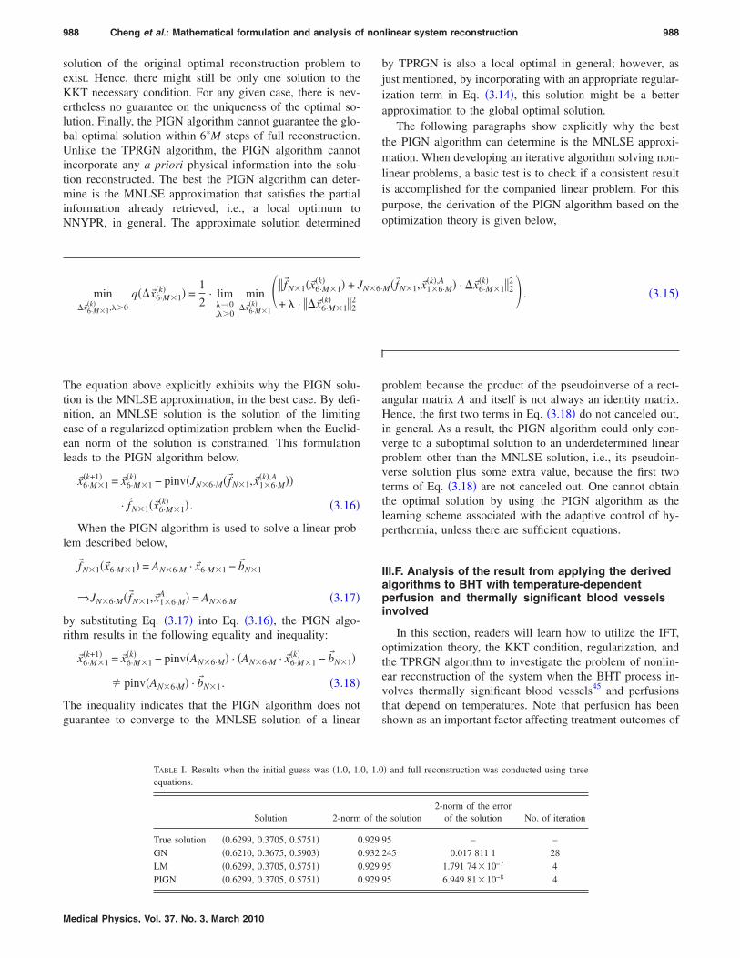

Page 9

988 Cheng et al.: Mathematical formulation and analysis of nonlinear system reconstruction 988

solution of the original optimal reconstruction problem toexist. Hence, there might still be only one solution to theKKT necessary condition. For any given case, there is nev-ertheless no guarantee on the uniqueness of the optimal so-lution. Finally, the PIGN algorithm cannot guarantee the glo-bal optimal solution within 6�M steps of full reconstruction.Unlike the TPRGN algorithm, the PIGN algorithm cannotincorporate any a priori physical information into the solu-tion reconstructed. The best the PIGN algorithm can deter-mine is the MNLSE approximation that satisfies the partialinformation already retrieved, i.e., a local optimum toNNYPR, in general. The approximate solution determined

Medical Physics, Vol. 37, No. 3, March 2010

by TPRGN is also a local optimal in general; however, asjust mentioned, by incorporating with an appropriate regular-ization term in Eq. �3.14�, this solution might be a betterapproximation to the global optimal solution.

The following paragraphs show explicitly why the bestthe PIGN algorithm can determine is the MNLSE approxi-mation. When developing an iterative algorithm solving non-linear problems, a basic test is to check if a consistent resultis accomplished for the companied linear problem. For thispurpose, the derivation of the PIGN algorithm based on theoptimization theory is given below,

minx�6·M�1

�k� , �0

q�x�6·M�1�k� � =

1

2· lim

→0, �0

minx�6·M�1

�k���f�N�1�x�6·M�1

�k� � + JN�6·M�f�N�1,x�1�6·M�k�,A � · x�6·M�1

�k� �22

+ · �x�6·M�1�k� �2

2 � . �3.15�

The equation above explicitly exhibits why the PIGN solu-tion is the MNLSE approximation, in the best case. By defi-nition, an MNLSE solution is the solution of the limitingcase of a regularized optimization problem when the Euclid-ean norm of the solution is constrained. This formulationleads to the PIGN algorithm below,

x�6·M�1�k+1� = x�6·M�1

�k� − pinv�JN�6·M�f�N�1,x�1�6·M�k�,A ��

· f�N�1�x�6·M�1�k� � . �3.16�

When the PIGN algorithm is used to solve a linear prob-lem described below,

f�N�1�x�6·M�1� = AN�6·M · x�6·M�1 − b�N�1

⇒JN�6·M�f�N�1,x�1�6·MA � = AN�6·M �3.17�

by substituting Eq. �3.17� into Eq. �3.16�, the PIGN algo-rithm results in the following equality and inequality:

x�6·M�1�k+1� = x�6·M�1

�k� − pinv�AN�6·M� · �AN�6·M · x�6·M�1�k� − b�N�1�

� pinv�AN�6·M� · b�N�1. �3.18�

The inequality indicates that the PIGN algorithm does notguarantee to converge to the MNLSE solution of a linear

TABLE I. Results when the initial guess was �1.0, 1.equations.

Solution 2-norm

True solution �0.6299, 0.3705, 0.5751� 0GN �0.6210, 0.3675, 0.5903� 0LM �0.6299, 0.3705, 0.5751� 0PIGN �0.6299, 0.3705, 0.5751� 0

problem because the product of the pseudoinverse of a rect-angular matrix A and itself is not always an identity matrix.Hence, the first two terms in Eq. �3.18� do not canceled out,in general. As a result, the PIGN algorithm could only con-verge to a suboptimal solution to an underdetermined linearproblem other than the MNLSE solution, i.e., its pseudoin-verse solution plus some extra value, because the first twoterms of Eq. �3.18� are not canceled out. One cannot obtainthe optimal solution by using the PIGN algorithm as thelearning scheme associated with the adaptive control of hy-perthermia, unless there are sufficient equations.

III.F. Analysis of the result from applying the derivedalgorithms to BHT with temperature-dependentperfusion and thermally significant blood vesselsinvolved

In this section, readers will learn how to utilize the IFT,optimization theory, the KKT condition, regularization, andthe TPRGN algorithm to investigate the problem of nonlin-ear reconstruction of the system when the BHT process in-volves thermally significant blood vessels45 and perfusionsthat depend on temperatures. Note that perfusion has beenshown as an important factor affecting treatment outcomes of

� and full reconstruction was conducted using three

e solution2-norm of the error

of the solution No. of iteration

95 – –245 0.017 811 1 2895 1.791 74�10−7 495 6.949 81�10−8 4

0, 1.0

of th

.929

.932

.929

.929

Page 10

989 Cheng et al.: Mathematical formulation and analysis of nonlinear system reconstruction 989

hyperthermia46–48,24 and, in practice, it can be affected bytemperature46,49,50 and thus makes the BHT process nonlin-ear.

III.F.1. Issues related to the problem formulation

The first and the most important step is to formulate theoutput temperature as a function of the input variables, e.g.,the 6�M variables representing the ensemble of the E fieldsfrom the M sources, plus a number of Madditional any othervariables, such as those parameters related to perfusion val-ues in different tissues. To make the formulation more ex-plicit, the Pennes BHTs with empirically curve-fitted perfu-

sion relations is employed to approximate temperature

tives of temperatures to unknowns.

Medical Physics, Vol. 37, No. 3, March 2010

response to nonlinear temperature-dependent perfusion. Inaddition, the convective heat transfer term is also included.The convective heat transfer from thermally significant bloodvessels is known to have strong influence onhyperthermia,45,51,52

� · Ct · � �T

�t+ u� · �T� = div�k grad�T�� − wb�T�

· Cb · �T − Tb� + Q . �3.19�

The vector u denotes the flow velocity vector inside the ther-mally significant vessel. The nonlinear curves expressed be-

48,13,9,12

low were used to simulate this phenomenon,

wtissue = �wtissue,1 + wtissue,2 exp�− �T − Tcrit,tissue�2

stissue�, T � Tcrit,tissue

wtissue,1 + wtissue,2, T � Tcrit,tissue

. �3.20�

Then, the nonlinear system is formulated in a form ofimplicit function below,

T = T�t,r�;E3�M,u� ,wtissue,1 · Cb,wtissue,2

· Cb,Tcrit,tissue,stissue,� · Ct,k� . �3.21�

The remaining steps for formulating the optimization prob-lem for the nonlinear reconstruction of the system, for deriv-ing the iterative search algorithm, and for analyzing the al-gorithm follow the same steps and patterns of Secs.III A–III E. In other words, all the conclusions drawn fromSecs. III A–III E remain valid for very general practical hy-perthermia with thermally significant vessels andtemperature-dependent perfusion.

III.F.2. Issues related to the calculation orestimation of the derivatives

As shown in Eq. �2.9�, the optimal solution to systemreconstruction problem using nonlinear formulation is deter-mined based on the KKT condition, and thus one needs todetermine the derivatives of temperatures to unknowns.Hence, it becomes essential for one to be able to determineexactly or approximately the derivatives of the temperaturesto the unknown variables.

However, in general, an explicit expression relating theunknown variables �e.g., those listed in the parentheses ofEq. �3.21�� and the temperatures is unavailable. The deriva-tives of the temperatures to the unknown variables are alsonot available. Two existing approaches were introduced be-low to address the determination or estimation of the deriva-

A remedy for the above mentioned situation is to solve thefollowing coupled partial differential equations �PDEs� forthe temperatures and the derivatives of the temperatures fromthe unknown variables,

� · Ct · � �T

�t+ u� · �T� = div�k grad�T�� − Db · �T − Tb�

+ Q,

Db � wb · Cb, �3.22�

� · Ct · � ��

�t+ u� · ��� = div�k grad���� − �T − Tb�

− Db · �,

� ��T

�Db. �3.23�

Equation �3.23� is the original PDE governing the BHTphysics. The new equation ��3.23�� shows up for the purposeof determining the unknown gradient required by the itera-tive algorithm such as GN or LM. Notice that even in thisvery simplified situation in which perfusion is a single con-stant, the approach requires one to solve the above system ofPDEs to determine the simulated temperatures and the asso-ciated derivatives. Furthermore, one should be aware that Eq.�3.23� is not linear. It is even more complicated, in practice,since perfusions are different in different tissues and followdifferent nonlinear dependences with temperatures �e.g., Eq.�3.20��. Plus, this computation for the set of coupled �non-linear� PDEs is required for every single iterative step of the

learning search for system reconstruction.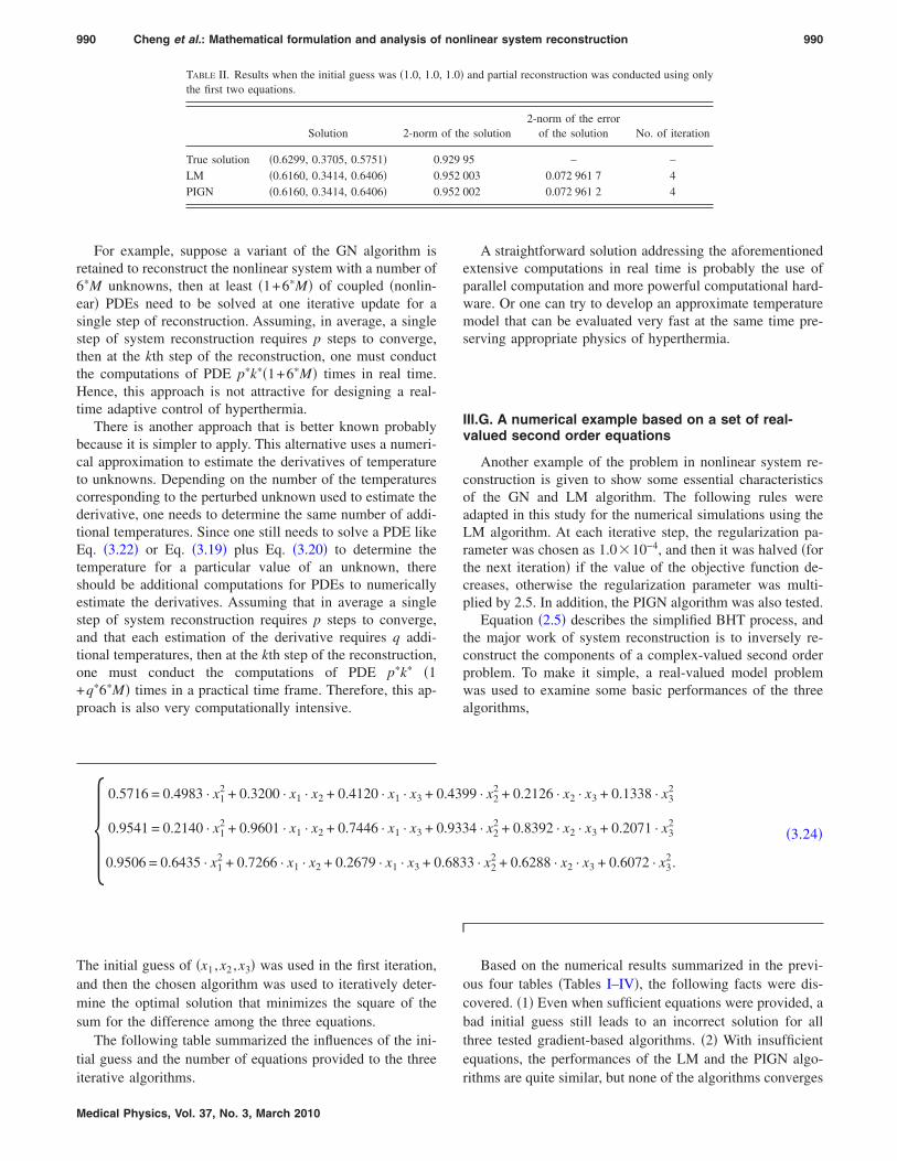

Page 11

990 Cheng et al.: Mathematical formulation and analysis of nonlinear system reconstruction 990

For example, suppose a variant of the GN algorithm isretained to reconstruct the nonlinear system with a number of6�M unknowns, then at least �1+6�M� of coupled �nonlin-ear� PDEs need to be solved at one iterative update for asingle step of reconstruction. Assuming, in average, a singlestep of system reconstruction requires p steps to converge,then at the kth step of the reconstruction, one must conductthe computations of PDE p�k��1+6�M� times in real time.Hence, this approach is not attractive for designing a real-time adaptive control of hyperthermia.

There is another approach that is better known probablybecause it is simpler to apply. This alternative uses a numeri-cal approximation to estimate the derivatives of temperatureto unknowns. Depending on the number of the temperaturescorresponding to the perturbed unknown used to estimate thederivative, one needs to determine the same number of addi-tional temperatures. Since one still needs to solve a PDE likeEq. �3.22� or Eq. �3.19� plus Eq. �3.20� to determine thetemperature for a particular value of an unknown, thereshould be additional computations for PDEs to numericallyestimate the derivatives. Assuming that in average a singlestep of system reconstruction requires p steps to converge,and that each estimation of the derivative requires q addi-tional temperatures, then at the kth step of the reconstruction,one must conduct the computations of PDE p�k� �1+q�6�M� times in a practical time frame. Therefore, this ap-

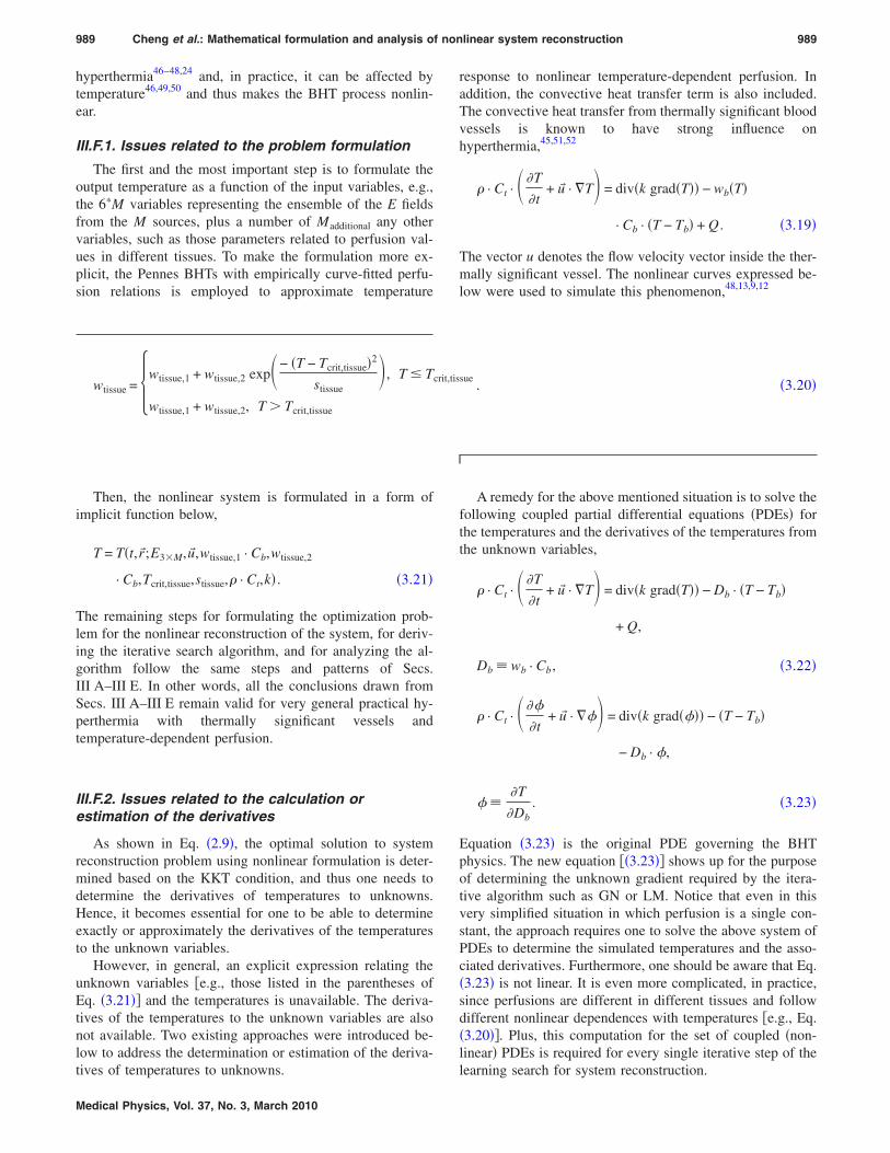
TABLE II. Results when the initial guess was �1.0, 1.0the first two equations.

Solution 2-norm

True solution �0.6299, 0.3705, 0.5751� 0LM �0.6160, 0.3414, 0.6406� 0PIGN �0.6160, 0.3414, 0.6406� 0

proach is also very computationally intensive.

iterative algorithms.

Medical Physics, Vol. 37, No. 3, March 2010

A straightforward solution addressing the aforementionedextensive computations in real time is probably the use ofparallel computation and more powerful computational hard-ware. Or one can try to develop an approximate temperaturemodel that can be evaluated very fast at the same time pre-serving appropriate physics of hyperthermia.

III.G. A numerical example based on a set of real-valued second order equations

Another example of the problem in nonlinear system re-construction is given to show some essential characteristicsof the GN and LM algorithm. The following rules wereadapted in this study for the numerical simulations using theLM algorithm. At each iterative step, the regularization pa-rameter was chosen as 1.0�10−4, and then it was halved �forthe next iteration� if the value of the objective function de-creases, otherwise the regularization parameter was multi-plied by 2.5. In addition, the PIGN algorithm was also tested.

Equation �2.5� describes the simplified BHT process, andthe major work of system reconstruction is to inversely re-construct the components of a complex-valued second orderproblem. To make it simple, a real-valued model problemwas used to examine some basic performances of the three

and partial reconstruction was conducted using only

e solution2-norm of the error

of the solution No. of iteration

95 – –003 0.072 961 7 4002 0.072 961 2 4

algorithms,

�0.5716 = 0.4983 · x1

2 + 0.3200 · x1 · x2 + 0.4120 · x1 · x3 + 0.4399 · x22 + 0.2126 · x2 · x3 + 0.1338 · x3

2

0.9541 = 0.2140 · x12 + 0.9601 · x1 · x2 + 0.7446 · x1 · x3 + 0.9334 · x2

2 + 0.8392 · x2 · x3 + 0.2071 · x32

0.9506 = 0.6435 · x12 + 0.7266 · x1 · x2 + 0.2679 · x1 · x3 + 0.6833 · x2

2 + 0.6288 · x2 · x3 + 0.6072 · x32.� �3.24�

The initial guess of �x1 ,x2 ,x3� was used in the first iteration,and then the chosen algorithm was used to iteratively deter-mine the optimal solution that minimizes the square of thesum for the difference among the three equations.

The following table summarized the influences of the ini-tial guess and the number of equations provided to the three

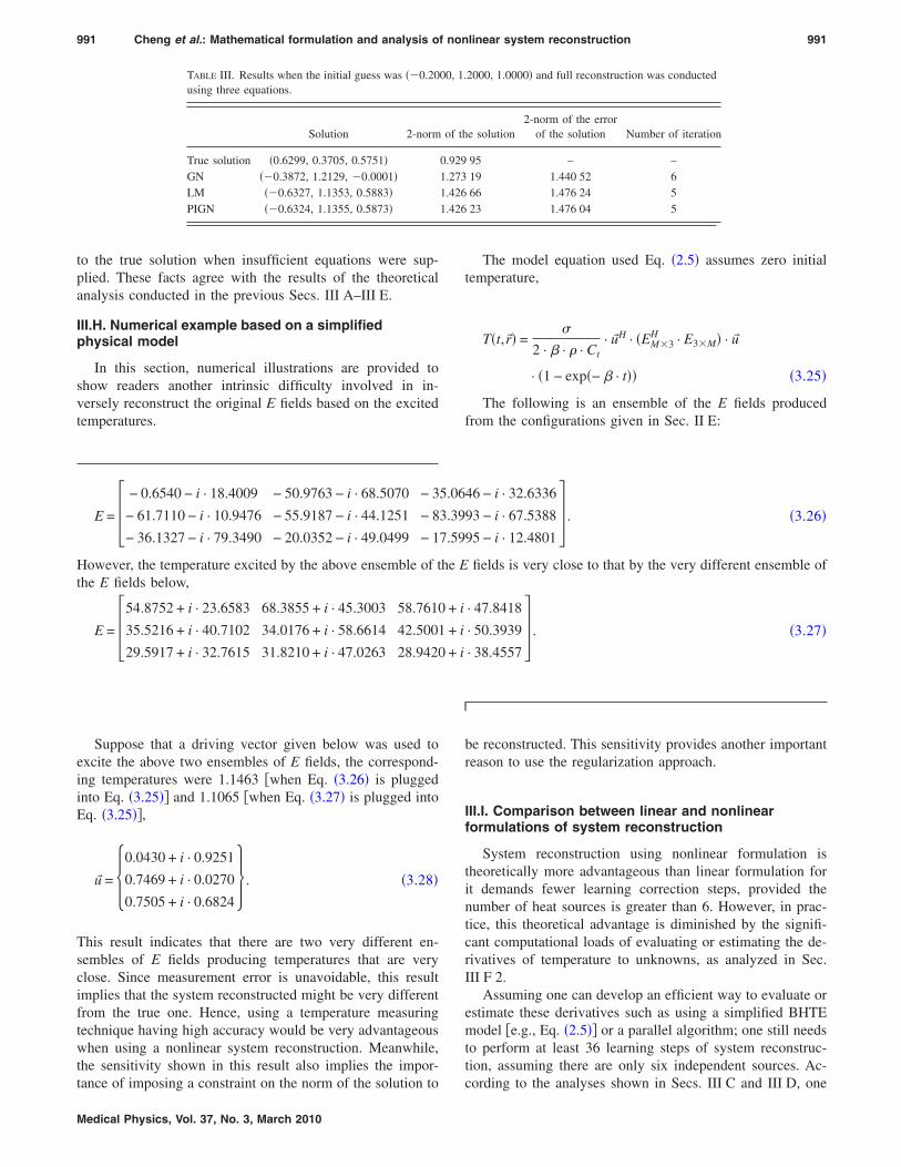
Based on the numerical results summarized in the previ-ous four tables �Tables I–IV�, the following facts were dis-covered. �1� Even when sufficient equations were provided, abad initial guess still leads to an incorrect solution for allthree tested gradient-based algorithms. �2� With insufficientequations, the performances of the LM and the PIGN algo-

, 1.0�

of th

.929

.952

.952

rithms are quite similar, but none of the algorithms converges

Page 12

991 Cheng et al.: Mathematical formulation and analysis of nonlinear system reconstruction 991

to the true solution when insufficient equations were sup-plied. These facts agree with the results of the theoreticalanalysis conducted in the previous Secs. III A–III E.

III.H. Numerical example based on a simplifiedphysical model

In this section, numerical illustrations are provided toshow readers another intrinsic difficulty involved in in-versely reconstruct the original E fields based on the excitedtemperatures.

TABLE III. Results when the initial guess was ��0.20using three equations.

Solution 2-norm

True solution �0.6299, 0.3705, 0.5751�GN ��0.3872, 1.2129, �0.0001�LM ��0.6327, 1.1353, 0.5883�PIGN ��0.6324, 1.1355, 0.5873�

tance of imposing a constraint on the norm of the solution to

Medical Physics, Vol. 37, No. 3, March 2010

The model equation used Eq. �2.5� assumes zero initialtemperature,

T�t,r�� =�

2 · � · � · Ct· u�H · �EM�3

H · E3�M� · u�

· �1 − exp�− � · t�� �3.25�

The following is an ensemble of the E fields producedfrom the configurations given in Sec. II E:

2000, 1.0000� and full reconstruction was conducted

e solution2-norm of the error

of the solution Number of iteration

95 – –19 1.440 52 666 1.476 24 523 1.476 04 5

E = − 0.6540 − i · 18.4009 − 50.9763 − i · 68.5070 − 35.0646 − i · 32.6336

− 61.7110 − i · 10.9476 − 55.9187 − i · 44.1251 − 83.3993 − i · 67.5388

− 36.1327 − i · 79.3490 − 20.0352 − i · 49.0499 − 17.5995 − i · 12.4801 . �3.26�

However, the temperature excited by the above ensemble of the E fields is very close to that by the very different ensemble ofthe E fields below,

E = 54.8752 + i · 23.6583 68.3855 + i · 45.3003 58.7610 + i · 47.8418

35.5216 + i · 40.7102 34.0176 + i · 58.6614 42.5001 + i · 50.3939

29.5917 + i · 32.7615 31.8210 + i · 47.0263 28.9420 + i · 38.4557 . �3.27�

Suppose that a driving vector given below was used toexcite the above two ensembles of E fields, the correspond-ing temperatures were 1.1463 �when Eq. �3.26� is pluggedinto Eq. �3.25�� and 1.1065 �when Eq. �3.27� is plugged intoEq. �3.25��,

u� = �0.0430 + i · 0.9251

0.7469 + i · 0.0270

0.7505 + i · 0.6824� . �3.28�

This result indicates that there are two very different en-sembles of E fields producing temperatures that are veryclose. Since measurement error is unavoidable, this resultimplies that the system reconstructed might be very differentfrom the true one. Hence, using a temperature measuringtechnique having high accuracy would be very advantageouswhen using a nonlinear system reconstruction. Meanwhile,the sensitivity shown in this result also implies the impor-

be reconstructed. This sensitivity provides another importantreason to use the regularization approach.

III.I. Comparison between linear and nonlinearformulations of system reconstruction

System reconstruction using nonlinear formulation istheoretically more advantageous than linear formulation forit demands fewer learning correction steps, provided thenumber of heat sources is greater than 6. However, in prac-tice, this theoretical advantage is diminished by the signifi-cant computational loads of evaluating or estimating the de-rivatives of temperature to unknowns, as analyzed in Sec.III F 2.

Assuming one can develop an efficient way to evaluate orestimate these derivatives such as using a simplified BHTEmodel �e.g., Eq. �2.5�� or a parallel algorithm; one still needsto perform at least 36 learning steps of system reconstruc-tion, assuming there are only six independent sources. Ac-

00, 1.

of th

0.9291.2731.4261.426

cording to the analyses shown in Secs. III C and III D, one

Page 13

992 Cheng et al.: Mathematical formulation and analysis of nonlinear system reconstruction 992

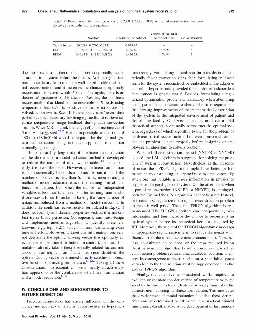
does not have a solid theoretical support to optimally recon-struct the true system before these steps. Adding regulariza-tion is mandatory to formulate a well-posed problem of par-tial reconstruction, and it increases the chance to optimallyreconstruct the system within 36 steps, but again, there is notheoretical guarantee of this success. Besides, the nonlinearreconstruction that identifies the ensemble of E fields usingtemperature feedbacks is sensitive to the perturbations in-volved, as shown in Sec. III H, and thus, a sufficient timeperiod becomes necessary for imaging facility to retrieve ac-curate temperature image feedback during each correctionsession. When MRI is used, the length of this time interval of5 min was suggested.53,15 Hence, in principle, a total time of180 min �180=5�36� would be required for the optimal sys-tem reconstruction using nonlinear approach; this is notclinically appealing.

This undesirably long time of nonlinear reconstructioncan be shortened if a model reduction method is developedto reduce the number of unknown variables,12 and appar-ently, the fewer the better. However, a nonlinear formulationis not theoretically better than a linear formulation, if thenumber of sources is less than 6. That is, incorporating amethod of model reduction reduces the learning time of non-linear formulation, but, when the number of independentvariables is less than 6, an even shorter learning time resultsif one uses a linear formulation having the same number ofunknowns reduced from a method of model reduction. Inaddition, the nonlinear reconstruction formulated in Eq. �2.4�does not identify any thermal properties such as thermal dif-fusivity or blood perfusion. Consequently, one must designand implement another algorithm to identify these un-knowns, e.g., Eq. �3.21�, which, in turn, demanding extratime and effort. However, without this information, one can-not determine the optimal driving vector that optimally el-evates the temperature distribution. In contrast, the linear for-mulation already taking these thermally related factors intoaccount in an implicit form,8 and thus, once identified, theoptimal driving vector determined directly satisfies an objec-tive function optimizing temperature.8,11,12 Taking all theseconsiderations into account, a more clinically attractive op-tion appears to be the combination of a linear formulationand a model reduction.11,12

IV. CONCLUSIONS AND SUGGESTIONS TOFUTURE DIRECTION

Problem formulation has strong influence on the effi-

TABLE IV. Results when the initial guess was ��0.2ducted using only the first two equations.

Solution 2-norm

True solution �0.6299, 0.3705, 0.5751�LM ��0.6327, 1.1353, 0.5883�PIGN ��0.6324, 1.1355, 0.5873�

ciency and accuracy of system reconstruction in hyperther-

Medical Physics, Vol. 37, No. 3, March 2010

mia therapy. Formulating in nonlinear form results in a theo-retically fewer correction steps than formulating in linearform for the system reconstruction embedded in the adaptivecontrol of hyperthermia, provided the number of independentheat sources is greater than 6. Besides, formulating a regu-larized optimization problem is mandatory when attemptingusing partial reconstruction to shorten the time required forthe learning improvements of the mathematical descriptionof the system to the integrated environment of patient andthe heating facility. Otherwise, one does not have a solidtheoretical support to optimally reconstruct the optimal sys-tem, regardless of which algorithm to use for the problem ofnonlinear partial reconstruction. In a word, one must formu-late the problem at hand properly before designing or em-ploying an algorithm to solve a problem.

When a full reconstruction method �NNLFR or NNYFR�is used, the LM algorithm is suggested for solving the prob-lem of system reconstruction. Nevertheless, in the presenceof noise, the TPRGN algorithm might have better perfor-mance in reconstructing an approximate system, especiallywhen one has reliable a priori information in physics tosupplement a good guessed system. On the other hand, whena partial reconstruction �NNLPR or NNYPR� is employed,both the LM and the GN algorithms cannot be used. Instead,one must first regularize the original reconstruction problemto make it well posed. Then, the TPRGN algorithm is rec-ommended. The TPRGN algorithm can incorporate a prioriinformation and thus increase the chance to reconstruct anoptimal system before its theoretical iterations required byIFT. Moreover, the users of the TPRGN algorithm can designan appropriate regularization term to reduce the negative in-fluences from the unavoidable measurement noise. Nonethe-less, an estimate, in advance, on the steps required by aniterative searching algorithm to solve a nonlinear partial re-construction problem remains unavailable. In addition, to en-sure its convergence to the true solution, a good initial guessvery close to the true solution must be supplemented with theLM or TPRGN algorithm.

Finally, the extensive computational works required toevaluate or estimate the derivatives of temperature with re-spect to the variables to be identified severely diminishes theattractiveness of using nonlinear formulation. This motivatesthe development of model reduction12 so that these deriva-tives can be determined or estimated in a practical clinical

1.2000, 1.0000� and partial reconstruction was con-

he solution2-norm of the error

of the solution No. of iteration

95 – –66 1.476 24 523 1.476 04 5

000,

of t

0.9291.4261.426

time frame. An alternative is the development of fast numeri-

Page 14

993 Cheng et al.: Mathematical formulation and analysis of nonlinear system reconstruction 993

cal solver to the Penne BHTE to accelerate the computationof the derivatives, e.g., implementing a parallel algorithm forthe BHTE.

ACKNOWLEDGMENTS

The authors thank Professor Robert Israel of the Depart-ment of Mathematics at the University of British Columbia,Canada, and Professor Elena Cherkaev of the Department ofMathematics at the University of Utah, USA for suggestions.The authors thank the comments and suggestions made bythe two reviewers, especially the suggestion made by the firstreviewer, in which the author was reminded to provide moredetailed explanations on the workloads required by linearand nonlinear learning algorithms. The authors also thankElisa H. Jenny, MSc, for the help on collecting literatures.This study was supported by NIH grant NCI P01—CA042745-23.

a�Author to whom correspondence should be addressed. Electronic mail:[email protected]; Telephone: 9196602169.

1E. Jones, D. Thrall, M. W. Dewhirst, and Z. Vujaskovic, “Prospectivethermal dosimetry: The key to hyperthermia’s future,” Int. J. Hyperther-mia 22, 247–253 �2006�.

2R. D. Issels, “High-risk soft tissue sarcoma: Clinical trial and hyperther-mia combined chemotherapy,” Int. J. Hyperthermia 22, 235–239 �2006�.

3J. Gellermann, B. Hildebrandt, R. Issels, H. Ganter, W. Wlodarczyk, V.Budach, R. Felix, P. U. Tunn, P. Reichardt, and P. Wust, “Noninvasivemagnetic resonance thermography of soft tissue sarcomas during regionalhyperthermia—Correlation with response and direct thermometry,” Can-cer 107, 1373–1382 �2006�.

4J. Gellermann, M. Weihrauch, C. H. Cho, W. Wlodarczyk, H. Fahling, R.Felix, V. Budach, M. Weiser, J. Nadobny, and P. Wust, “Comparison ofMR-thermography and planning calculations in phantoms,” Med. Phys.33, 3912–3920 �2006�.

5P. Wust, C. H. Cho, B. Hildebrandt, and J. Gellermann, “Thermal moni-toring: Invasive, minimal-invasive and non-invasive approaches,” Int. J.Hyperthermia 22, 255–262 �2006�.

6S. A. Goss, R. L. Johnston, and F. Dunn, “Comprehensive compilation ofempirical ultrasonic properties of mammalian tissues,” J. Acoust. Soc.Am. 64, 423–457 �1978�.

7S. Gabriel, R. W. Lau, and C. Gabriel, “The dielectric properties of bio-logical tissues. III. Parametric models for the dielectric spectrum of tis-sues,” Phys. Med. Biol. 41, 2271–2293 �1996�.

8K.-S. Cheng, V. Stakhursky, P. R. Stauffer, M. W. Dewhirst, and S. K.Das, “Online feedback focusing algorithm for hyperthermia cancer treat-ment,” Int. J. Hyperthermia 23, 539–554 �2007�.

9K.-S. Cheng, V. Stakhursky, O. I. Craciunescu, P. Stauffer, M. Dewhirst,and S. K. Das, “Fast temperature optimization of multi-source hyperther-mia applicators with reduced-order modeling of ‘virtual sources’,” Phys.Med. Biol. 53, 1619–1635 �2008�.

10M. Seebass, R. Beck, J. Gellermann, J. Nadobny, and P. Wust, “Electro-magnetic phased arrays for regional hyperthermia: Optimal frequency andantenna arrangement,” Int. J. Hyperthermia 17, 321–336 �2001�.

11K.-S. Cheng, Y. Yuan, Z. Li, P. R. Stauffer, W. T. Joines, M. W. Dewhirst,and S. K. Das, “Control time reduction using virtual source projection fortreating a leg sarcoma with nonlinear perfusion,” SPIE Photonics West,San Jose, CA, 24–29 January 2009, Vol. 7181 �unpublished�.

12K.-S. Cheng, Y. Yuan, Z. Li, P. R. Stauffer, P. Maccarini, W. T. Joines, M.W. Dewhirst, and S. K. Das, “Performance of a reduced-order adaptivecontroller when used in multi-antenna hyperthermia treatments with non-linear temperature-dependent perfusion,” Phys. Med. Biol. 54, 1979–1995�2009�.

13M. E. Kowalski and J.-M. Jin, “A temperature-based feedback controlsystem for electromagnetic phased-array hyperthermia: Theory and simu-lation,” Phys. Med. Biol. 48, 633–651 �2003�.

14K.-S. Cheng, M.W. Dewhirst, P. R. Stauffer, and S. Das, “Effective learn-ing strategies for real-time image-guided adaptive control of multiple

source hyperthermia applicators,” Med. Phys. 37 �2010�.

Medical Physics, Vol. 37, No. 3, March 2010

15M. Weihrauch, P. Wust, M. Weiser, J. Nadobny, S. Eisenhardt, V. Budach,and J. Gellermann, “Adaptation of antenna profiles for control of MRguided hyperthermia �HT� in a hybrid MR-HT system,” Med. Phys. 34,4717–4725 �2007�.

16G. Dorfleitner, P. Schneider, K. Hawlitschek, and A. Buch, “Pricing op-tions with Green’s functions when volatility, interest rate and barriersdepend on time,” Quant. Finance 8, 119–133 �2008�.

17P. Fotiu, “Integral equation analysis of elastic-viscoplastic fracturingplates under dynamic loading,” Proceedings of the Second InternationalConference on Computational Plasticity, Models, Software and Applica-tions �Pineridge, Swansea, 1989�, pp. 1171–1182.

18A. El-Azab and N. M. Ghoniem, “Green’s function for the elastic field ofan edge dislocation in a finite orthotropic medium,” Int. J. Fract. 61,17–37 �1993�.

19C. Toepffer and C. Cercignani, “Analytical results for the Boltzmannequation,” Contrib. Plasma Phys. 37, 279–291 �1997�.

20C. A. Balanis, Advanced Engineering Electromagnetics �Wiley, NewYork, 1989�, Solution Manual ed.

21H. H. Pennes, “Analysis of tissue and arterial blood temperatures in theresting human forearm,” J. Appl. Physiol. 1, 93–122 �1948�.

22K.-S. Cheng and R. B. Roemer, “Closed-form solution for the thermaldose delivered during single pulse thermal therapies,” Int. J. Hyperther-mia 21, 215–230 �2005�.

23R. B. Roemer, “The local tissue cooling coefficient: A unified approach tothermal washout and steady-state ‘perfusion’ calculation,” Int. J. Hyper-thermia 6, 421–430 �1990�.

24K.-S. Cheng and R. B. Roemer, “Blood perfusion and thermal conductioneffects in Gaussian beam, minimum time single-pulse thermal therapies,”Med. Phys. 32, 311–317 �2005�.

25L. Cesari, “The implicit function theorem in functional analysis,” DukeMath. J. 33, 417–440 �1966�.

26T. H. McNicholl, “Computability and the implicit function theorem,”Electron. Notes Theor. Comput. Sci. 167, 3–15 �2007�.

27H. W. Kuhn and A. W. Tucker, presented at the Proceedings of the Sec-ond Berkeley Symposium, Berkeley, CA, 1951, pp. 481–492 �unpub-lished�.

28C. Gabriel, S. Gabriel, and E. Corthout, “The dielectric properties ofbiological tissues. I. Literature survey,” Phys. Med. Biol. 41, 2231–2249�1996�.

29S. Gabriel, R. W. Lau, and C. Gabriel, “The dielectric properties of bio-logical tissues. II. Measurements in the frequency range 10 Hz to 20GHz,” Phys. Med. Biol. 41, 2251–2269 �1996�.

30W. H. Hayt, Jr. and J. A. Buck, Engineering Electromagnetics, 7th ed.�McGraw-Hill Higher Education, New York, 2006�.

31C. A. T. Van den Berg, J. B. Van De Kamer, A. A. C. De Leeuw, C. R. L.P. N. Jeukens, B. W. Raaymakers, M. Van Vulpen, and J. J. W. Lagendijk,“Towards patient specific thermal modelling of the prostate,” Phys. Med.Biol. 51, 809–825 �2006�.

32C. F. Gauss, Theory of the motion of the heavenly bodies moving aboutthe sun in conic sections �Dover, New York, 1963�.

33P. Deuflhard and V. Apostolescu, Amsterdam, Netherlands, 1980 �unpub-lished�.

34K. Levenberg, “A method for the solution of certain non-linear problemsin least squares,” Q. Appl. Math. 2, 164–168 �1944�.

35D. Marquardt, “An algorithm for least-squares estimation of nonlinearparameters,” SIAM J. Appl. Math. 11, 431–441 �1963�.

36P. Wust, H. Fahling, W. Wlodarczyk, M. Seebass, J. Gellermann, P. Deu-flhard, and J. Nadobny, “Antenna arrays in the SIGMA-eye applicator:Interactions and transforming networks,” Med. Phys. 28, 1793–1805�2001�.

37J. Hadamard, “Sur les problemes aux derivees partielles et leur significa-tion physique,” Princeton University Bulletin 13, 49–52 �1902�.

38D. L. Philips, “A technique for numerical solution of certain integralequations of the first kind,” J. Assoc. Comput. Mach. 9, 84–97 �1962�.

39A.-I. N. Tikhonov, “Regularization of incorrectly posed problems,” Sov.Math. Dokl. 4, 1624–1627 �1963�.

40C. M. Leung and W.-S. Lu, presented at the Proceedings of the CanadianConference on Electrical and Computer Engineering, Vancouver, BC,Canada, 14–17 September 1993 �unpublished�.

41U. Amato and W. Hughes, “Maximum entropy regularization of Fred-holm integral equations of the first kind,” Inverse Probl. 7, 793–808�1991�.

42

T. Schröter and U. Tautenhahn, “Error estimates for Tikhonov regulariza-

Page 15

994 Cheng et al.: Mathematical formulation and analysis of nonlinear system reconstruction 994

tion in Hilbert scales,” Numer. Funct. Anal. Optim. 15, 155–168 �1994�.43E. H. Moore, “On the reciprocal of the general algebraic matrix,” Bull.

Am. Math. Soc. 26, 394–395 �1920�.44R. Penrose, presented at the Proceedings of the Cambridge Philosophical

Society, 1955 �unpublished�.45J. W. Baish, P. S. Ayyaswamy, and K. R. Foster, “Heat transport mecha-

nisms in vascular tissues: A model comparison,” J. Biomech. Eng. 108,324–331 �1986�.

46C. W. Song, A. Lokshina, J. G. Rhee, M. Patten, and S. H. Levitt, “Im-plication of blood flow in hyperthermia treatment of tumors,” IEEE Trans.Biomed. Eng. BME-31, 9–16 �1984�.

47D. T. Tompkinsn, R. Vanderby, S. A. Klein, W. A. Beckman, D. M.Steeves, D. M. Frey, and B. R. Palival, “Temperature-dependent versusconstant rate blood perfusion modeling in ferromagnetic thermoseed hy-perthermia,” Int. J. Hyperthermia 10, 517–536 �1994�.

48J. Lang, B. Erdmann, and M. Seebass, “Impact of nonlinear heat transfer

on temperature control in regional hyperthermia,” IEEE Trans. Biomed.

Medical Physics, Vol. 37, No. 3, March 2010

Eng. 46, 1129–1138 �1999�.49R. B. Roemer, J. R. Oleson, and T. C. Cetas, “Oscillatory vasoactivity

response to constant power,” Am. J. Physiol. 249, R153–R158 �1985�.50D. Akyürekli, L. H. Gerig, and G. P. Raaphorst, “Changes in muscle

blood flow distribution during hyperthermia,” Int. J. Hyperthermia 13,481–496 �1997�.

51J. Song, L. X. Xu, D. E. Lemons, and S. Weinbaum, “Enhancement in theeffective thermal conductivity in rat spinotrapezius due to vasoregula-tion,” J.Biomech. Eng. 119, 461–468 �1997�.

52D. Shrivastava and R. B. Roemer, “Readdressing the issue of thermallysignificant blood vessels using a countercurrent vessel network,” J. Bio-mech. Eng. 128, 210–216 �2006�.

53J. Nadobny, W. Wlodarczyk, L. Westhoff, J. Gellermann, R. Felix, and P.Wust, “A clinical water-coated antenna applicator for MR-controlleddeep-body hyperthermia: A comparison of calculated and measured 3-D

temperature data sets,” IEEE Trans. Biomed. Eng. 52, 505–519 �2005�.