Mathematica Laboratories for Mathematical Statistics: Emphasizing Simulation and Computer Intenstive Methods by Jenny A. Baglivo ASA-SIAM Series on Statistics and Applied Probability Copyright (c) 2005-2012 by the American Statistical Association and the Society for Industrial and Applied Mathematics Mathematica Laboratories for Mathematical Statistics introduces an approach to incorporating technology in the mathe- matical statistics sequence, with an emphasis on simulation and computer intensive methods. The printed book is a concise introduction to the concepts of probability theory and mathematical statistics. The accompanying electronic materials are a series of in-class and take-home computer laboratory problems designed to reinforce the concepts, and to apply the techniques in real and realistic settings. The original laboratory materials were written for Mathematica Version 5, and have been updated for Version 7. The materials are designed so that students with little or no experience in Mathematica will be able to complete the work. The materials are written to be used in the mathematical statistics sequence given at most colleges and universities (two courses of four semester hours each or three courses of three semester hours each). Multivariable calculus, and familiarity with the basics of set theory, vectors and matrices, and problem-solving using a computer are assumed. The order of topics generally follows that of a standard sequence. Chapters 1 through 5 cover concepts in probability. Chapters 6 through 10 cover introductory mathematical statistics. Chapters 11 and 12 are on permutation and bootstrap methods; in each case, problems are designed to expand on ideas from previous chapters so that instructors could choose to use some of the problems earlier in the course. Permutation and bootstrap methods also appear in the later chapters. Chapters 13, 14 and 15 are on multiple sample analysis, linear least squares and contingency tables, respectively. References for special- ized topics in Chapters 10 through 15 are given at the beginning of each chapter. Each chapter has a main laboratory notebook containing between five and seven problems, and a series of additional problem notebooks. The problems in the main laboratory notebook are for basic understanding, and can be used for in- class work or assigned for homework. The additional problem notebooks reinforce and/or expand the ideas from the main laboratory notebook and are generally longer and more involved. This PDF file contains (I) The main laboratory notebook for Chapter 14 (linear least squares analysis), pages 2-11; (II) Typical output from the examples in the notebook, pages 12-17; and (III) Solutions to the problems in the notebook, pages 18-26. Copyright © by the Society for Industrial and Applied Mathematics Unauthorized reproduction of this article is prohibited.

Welcome message from author
This document is posted to help you gain knowledge. Please leave a comment to let me know what you think about it! Share it to your friends and learn new things together.
Transcript

Mathematica Laboratories for Mathematical Statistics:Emphasizing Simulation and Computer Intenstive Methods
by Jenny A. Baglivo
ASA-SIAM Series on Statistics and Applied ProbabilityCopyright (c) 2005-2012 by the American Statistical Association andthe Society for Industrial and Applied Mathematics
Mathematica Laboratories for Mathematical Statistics introduces an approach to incorporating technology in the mathe-matical statistics sequence, with an emphasis on simulation and computer intensive methods. The printed book is aconcise introduction to the concepts of probability theory and mathematical statistics. The accompanying electronicmaterials are a series of in-class and take-home computer laboratory problems designed to reinforce the concepts, and toapply the techniques in real and realistic settings. The original laboratory materials were written for MathematicaVersion 5, and have been updated for Version 7. The materials are designed so that students with little or no experiencein Mathematica will be able to complete the work.
The materials are written to be used in the mathematical statistics sequence given at most colleges and universities (twocourses of four semester hours each or three courses of three semester hours each). Multivariable calculus, and familiaritywith the basics of set theory, vectors and matrices, and problem-solving using a computer are assumed. The order oftopics generally follows that of a standard sequence. Chapters 1 through 5 cover concepts in probability. Chapters 6through 10 cover introductory mathematical statistics. Chapters 11 and 12 are on permutation and bootstrap methods; ineach case, problems are designed to expand on ideas from previous chapters so that instructors could choose to use someof the problems earlier in the course. Permutation and bootstrap methods also appear in the later chapters. Chapters 13, 14and 15 are on multiple sample analysis, linear least squares and contingency tables, respectively. References for special-ized topics in Chapters 10 through 15 are given at the beginning of each chapter.
Each chapter has a main laboratory notebook containing between five and seven problems, and a series of additionalproblem notebooks. The problems in the main laboratory notebook are for basic understanding, and can be used for in-class work or assigned for homework. The additional problem notebooks reinforce and/or expand the ideas from the mainlaboratory notebook and are generally longer and more involved.
This PDF file contains
(I) The main laboratory notebook for Chapter 14 (linear least squares analysis), pages 2-11;
(II) Typical output from the examples in the notebook, pages 12-17; and
(III) Solutions to the problems in the notebook, pages 18-26.
Copyright © by the Society for Industrial and Applied Mathematics Unauthorized reproduction of this article is prohibited.

Part I. Laboratory 14: Linear Least Squares
§1. Simple Linear Least Squares
Assume that the response random variable Y can be written as a linear function of the form
Y = a + b X + e
where
• the predictor X and the error e are independent random variables,• The distribution of e has mean 0 and standard deviation s, and • All parameters (a, b, s) are unknown.
Then the conditional expectation of Y given X = x is a linear function in x
E HY X = xL = a + b x
and the standard deviation of the conditional distribution does not depend on x.
This section focuses on least squares and permutation methods to estimate the parameters in the conditional mean formulausing the Fit and SlopeCI functions. Please evaluate the following command before starting your work.
Needs@"StatTools`Group1`"D;Needs@"StatTools`Group2`"D;Needs@"StatTools`Group3`"D;Needs@"StatTools`Group4`"D;
The form of the Fit function is as follows:
Fit[pairs,{1,x},x]returns the estimated mean formula, where pairs is a list of pairs of real numbers.
Note: The pairs are assumed to be the values of a random sample from the joint (X, Y) distribution or to have beengenerated independently from conditional distributions at fixed values of X.
Example 1:
To illustrate the use of the Fit function using simulation, let X be a uniform random variable on the interval [0, 50], e bea uniform random variable on the interval [|25, 25] and
Y = 2 - 3 X + e .
(1) Evaluate the following command to construct a list of 80 pairs from the joint (X, Y) distribution.
nn = 80;xvals = RandomReal@UniformDistribution@80, 50<D, nnD;evals = RandomReal@UniformDistribution@8-25, 25<D, nnD;
yvals = 2 - 3 * xvals + evals;pairs = Transpose@8xvals, yvals<D;
The y-coordinates (yvals) are a linear function of the x-coordinates (xvals) and a random sample from the error distribu-tion (evals).
(2) Evaluate the following command to construct a scatter plot of the observations and to display the sample correlation.
2 SA14SampleLab.nb
Copyright © by the Society for Industrial and Applied Mathematics Unauthorized reproduction of this article is prohibited.

ScatterPlot@pairs,Correlation Ø TrueD
There is a strong negative association between X and Y.
(3) Evaluate the following command to define a function, f, whose value at x is the estimated conditional mean.
Clear@xD; Remove@fD;f@x_D = Fit@pairs, 81, x<, xD
Fit uses the pairs list to find least squares estimates of intercept and slope (the coefficients of 1 and x, respectively) as afunction of x. The estimated formula is stored as the value of f(x). The graph of y = f(x) is the gray line in the scatter plotin step (2).
(4) Repeat the commands in steps (1) through (3) several times to see different plots and estimates of the conditionalexpectation. Then repeat the simulation several times each assuming the error distribution is uniform on the interval [|5,+5] and assuming it is uniform on the interval [|100, +100]. In the first case, the correlations will be very close to |1 andthe estimated formulas close to 2|3x. In the second case, the correlations will be close to |0.60 and the estimated formu-las will be much more variable.
ü Permutation confidence interval for b
Permutation methods can be used to construct 100(1|g)% confidence intervals for the slope parameter b. A value b0 is inthe confidence interval if the two sided test of
H0 : The correlation between X and Y - b0 X equals zero
accepts H0 at the g significance level. The SlopeCI function uses simulation to approximate the permutationconfidence interval:
SlopeCI[pairs,ConfidenceLevelØ1-g,RandomPermutationsØr]returns an approximate 100(1-g)% permutation confidence interval for the slope based on r random permutations, where pairs is a list of pairs of numbers.
Note: If the options are omitted, then SlopeCI returns an approximate 95% permutation confidence interval based on1000 random permutations.
Example 1, continued:
Evaluate the first command to initialize a list of 80 pairs from the joint (X, Y) distribution defined above. Evaluate thesecond command to construct an approximate 95% confidence interval for b using 2000 random permutations.
nn = 80;xvals = RandomReal@UniformDistribution@80, 50<D, nnD;evals = RandomReal@UniformDistribution@8-25, 25<D, nnD;yvals = 2 - 3 * xvals + evals;pairs = Transpose@8xvals, yvals<D;
SlopeCI@pairs, RandomPermutations Ø 2000D
Repeat the commands several times. The computed interval will contain b = -3 with probability approximately 0.95.
Problem 1: Assume that X and e are independent uniform random variables, the range of X is [0, 80], and the range of e is [|50, +50]. Let Y = 2 - 3 X + e.
(a) Generate a random sample (pairs) of size 100 from the joint (X, Y) distribution. For these data,
• Compute the sample mean and sample standard deviation of the x- and y-coordinates. • Construct a scatter plot of the pairs and display the sample correlation.• Use Fit to estimate the conditional expectation.• Use SlopeCI to construct an approximate 95% confidence interval for the slope based on 2000 random permutations. Is |3 in the interval?
SA14SampleLab.nb 3
Copyright © by the Society for Industrial and Applied Mathematics Unauthorized reproduction of this article is prohibited.

Problem 1: Assume that X and e are independent uniform random variables, the range of X is [0, 80], and the range of e is [|50, +50]. Let Y = 2 - 3 X + e.
(a) Generate a random sample (pairs) of size 100 from the joint (X, Y) distribution. For these data,
• Compute the sample mean and sample standard deviation of the x- and y-coordinates. • Construct a scatter plot of the pairs and display the sample correlation.• Use Fit to estimate the conditional expectation.• Use SlopeCI to construct an approximate 95% confidence interval for the slope based on 2000 random permutations. Is |3 in the interval?
(b) Compute E(X), SD(X), E(Y), SD(Y), and r = Corr(X,Y). Are the sample summaries (the sample means, standard deviations, and correlation) from part (a) close to these model summaries?
Example 2:
As part of a study on sleep in mammals, researchers collected information on the average brain and body weights for 43different species. The graph below compares the common logarithms of average brain weight in grams (vertical axis) andaverage body weight in kilograms (horizontal axis) for the 43 species. The largest log-average brain weight (the greendot) corresponds to the Asian elephant; the second largest (the red dot) to man. The gray line is the least squares linear fitto the paired data. (Sources: Allison and Cicchetti, 1976; lib.stat.cmu.edu/DASL.)
-2 -1 0 1 2 3 4log10HwbL
-1
0
1
2
3
4
log10HwbrL
Common logs of average brain (vertical axis) and body (horizontal axis) weights for 43 species of mammals.
The lists species, wbody, and wbrain give the species names (listed alphabetically) and corresponding body and brainweights.
species, wbody, wbrain are lists of length 43.
Body weights range from 0.005 kg (0.18 ounces) to 2547.0 kg (5,615.12 pounds). Brain weights range from 0.14 g(0.004 ounces) to 4603.0 g (10.15 pounds). To initialize the data, click on the rightmost bracket of the cell above andevaluate the command.
(1) Evaluate the following command to construct the list of pairs displayed above.
pairs = Transpose@8Log@10, wbodyD, Log@10, wbrainD<D;
Note that the common logarithm is the logarithm function with base 10.
(2) Evaluate the following command to display a table of the paired data along with the species names.
TableFormApairs,
TableHeadings Ø 9species, 9"log10HwbL", "log10HwbrL"==E
Problem 2: (a) Using the paired (log-body weight, log-brain weight) data,
• Use Fit to find the least squares estimate of the conditional expectation of log-brain weight given log-body weight. • Use SlopeCI to construct an approximate 95% confidence interval for the slope.• Interpret the estimated slope in the context of the brain-body problem.
4 SA14SampleLab.nb
Copyright © by the Society for Industrial and Applied Mathematics Unauthorized reproduction of this article is prohibited.

Problem 2: (a) Using the paired (log-body weight, log-brain weight) data,
• Use Fit to find the least squares estimate of the conditional expectation of log-brain weight given log-body weight. • Use SlopeCI to construct an approximate 95% confidence interval for the slope.• Interpret the estimated slope in the context of the brain-body problem.
(b) One of our mammalian cousins, the gorilla, has been left off the list of species. The gorilla has an average body weight of 207.0 kg (456.35 pounds) and an average brain weight of 406.0 g (14.32 ounces).
Use the least squares formula from part (a) to estimate the gorilla's average brain weight from its average body weight. Is the estimated average brain weight close to the true average brain weight?
(c) Use the least squares formula from part (a) to define a function g whose input is an average body weight and whose output is an estimate of the average brain weight. Then evaluate the command below to produce a smoothed scatter plot of (wb,wbr) pairs with the graph of y = gHxL superimposed. Comment on the plot.
pairs2 = Transpose@8wbody, wbrain<D;SmoothPlot@8pairs2, g<,AxesLabel Ø 8"wb", "wbr"<D
Note: SmoothPlot generalizes ScatterPlot with the CorrelationØTrue option. It is used to visualize non-linear relationships. Evaluate the command ?SmoothPlot to obtain information on this function.
§ 2. Linear Regression Analysis
Assume that the response random variable Y can be written as a linear function of the form
Y = b0 + b1 X1 + b2 X2 + . . . + bp-1 Xp-1 + e
where
• The error random variable, e, is independent of each predictor, Xi, • e is a normal random variable with mean 0 and standard deviation s, and• All p+1 parameters (the bi's and s) are unknown.
Let
X = I1, X1, X2, . . . , Xp-1M
represent the list including the constant 1 and the p|1 predictors (the p basis functions).
Then the conditional expectation of Y given X = x is a linear function:
E HY X = xL = b0 + b1 x1 + b2 x2 + . . . + bp-1 xp-1
and the conditional distribution is normal with standard deviation s.
This section focuses on using least squares methods to estimate the parameters in the conditional mean formula using theFit and LinearModelFit functions. The forms of the functions are as follows:
Fit[cases,functions,variables]returns the estimated mean formula, where cases is the list of observations, functions is the list of p basis functions, and variables is a single variable or a list of variables needed in the formula.
LinearModelFit[cases,functions,variables]returns a fitted linear model whose mean formula is estimated using least squares methods.
SA14SampleLab.nb 5
Copyright © by the Society for Industrial and Applied Mathematics Unauthorized reproduction of this article is prohibited.

LinearModelFit[cases,functions,variables]returns a fitted linear model whose mean formula is estimated using least squares methods.
Notes:(1) The predictors, Xi, may be single variables or functions of one or more variables. For numerical
stability, the predictors should not be strongly correlated.(2) If there are k variables, then each case must be a list of k+1 numbers (k variables plus response). The p
basis functions must be functions of the k variables only. (3) The following properties of fitted linear models will be used in the section: ANOVATable,
ANOVATableSumsOfSquares, ParameterConfidenceTable, RSquared, EstimatedVariance, StandardizedResiduals. Additional properties will be considered in Section 3.
(4) See the Help Browser for additional information about the LinearModelFit function.
Example 3:
To illustrate the analysis using simulation, assume that X is a uniform random variable on the interval [0, 20], e is anormal random variable with mean 0 and standard deviation 8, and X and e are independent. Let
Y = 40 - 15 X + 0.60 X2 + e = -50 - 3 HX - 10L + 0.60 HX - 10L2 + e.
(1) Evaluate the following command to construct a list of 100 cases from the joint (X, Y) distribution.
nn = 100;xvals = RandomReal@UniformDistribution@80, 20<D, nnD;evals = RandomReal@NormalDistribution@0, 8D, nnD;yvals = 40 - 15 * xvals + 0.60 * xvals^2 + evals;cases = Transpose@8xvals, yvals<D;
The y-coordinates are generated using the first form of the linear equation.
(2) Evaluate the following command to use Fit to estimate the conditional expectation of Y given X = x using thepredictors for the second form of the linear equation.
Clear@xD; Remove@fD;f@x_D = Fit@cases, 81, x - 10, Hx - 10L^2<, xD
The estimated formula is stored as the value of f(x).
(3) Evaluate the following command to construct a scatter plot of the cases list with the estimated conditional expectationsuperimposed.
SmoothPlot@8cases, f<D
The least squares estimate is likely to approximate the observed pairs quite well. (If the standard deviation of e was 28instead of 8, for example, the fit might not so close.)
Problem 3: Let X be a uniform random variable on the interval [0, 20]. Compute
• The correlation between X and X2.• The correlation between (X | 10) and HX - 10L2.
ü Analysis of variance
Let N be the number of cases, p be the number of functions,
• xi and Yi (i = 1, 2, . . . , N) be the N observed predictor lists and responses, respectively,
6 SA14SampleLab.nb
Copyright © by the Society for Industrial and Applied Mathematics Unauthorized reproduction of this article is prohibited.
• xi and Yi (i = 1, 2, . . . , N) be the N observed predictor lists and responses, respectively, • f(xi) (i = 1, 2, . . . , N) be the estimated means (or predicted responses), and
• Y be the mean response.
A test of the null hypothesis that the regression effects are identically zero (or b j = 0 for j > 0) has three sources ofvariation, as outlined in the following table:
DF SumOfSq MeanSq
Model p - 1 SSm =⁄i If HxiL - YM2 MSm = SSm ê Hp - 1L
Error N - p SSe = ⁄i HYi - f HxiLL2 MSe = SSe ê HN - pL
Total N - 1 SSt = ⁄i IYi - YM2
If the null hypothesis is true, then the ratio F = MSm êMSe has an f ratio distribution with p - 1 and N - p degrees offreedom. Large values of F provide evidence that the proposed predictors have some predictive value.
Example 3, continued
(1) Evaluate the following command to initialize a list of 100 cases from the joint (X, Y) distribution above.
nn = 100;xvals = RandomReal@UniformDistribution@80, 20<D, nnD;evals = RandomReal@NormalDistribution@0, 8D, nnD;yvals = 40 - 15 * xvals + 0.60 * xvals^2 + evals;cases = Transpose@8xvals, yvals<D;
(2) Evaluate the following two commands to construct a linear model (lm) based on this list and to retrieve an extendedANOVA table.
Clear@xD;lm = LinearModelFit@cases, 81, Hx - 10L, Hx - 10L^2<, 8x<D;
lm@"ANOVATable"D
The extended ANOVA table provided by Mathematica provides information about each predictor function (the first twolines), but does not provide the overall test we need.
(3) Evaluate the following command to retrieve the sums of squares column from the extended ANOVA table. Thecolumn consists of the sums of squares for the two predictor functions (ss1, ss2), the error sum of squares (sse), and thetotal sum of squares (sst).
8ss1, ss2, sse, sst< = lm@"ANOVATableSumsOfSquares"D
The model sum of squares is the sum of the first two elements of this list.
(4) Evaluate the first command to return the f ratio statistic (fstatistic) needed for the analysis. Evaluate the secondcommand to return the p value for the test of the predictive value of the given predictors.
p = 3;ssm = ss1 + ss2;fstatistic = Hssm ê Hp - 1LL ê Hsse ê Hnn - pLL
pvalue = 1 - CDF@FRatioDistribution@p - 1, nn - pD, fstatisticD
The p value is likely to be virtually zero.
(4) Evaluate the following command to retrieve the coefficient of determination, R2.
lm@"RSquared"D
R2 = SSm êSSt is the proportion of the total variation explained by the proposed model. Approximately 90% of the totalvariation is explained by the model in this case. (Note that as s increases, the value of R2generally decreases.)
SA14SampleLab.nb 7
Copyright © by the Society for Industrial and Applied Mathematics Unauthorized reproduction of this article is prohibited.

R2 = SSm êSSt is the proportion of the total variation explained by the proposed model. Approximately 90% of the totalvariation is explained by the model in this case. (Note that as s increases, the value of R2generally decreases.)
ü Parameter estimates and standardized residuals
We next examine 95% confidence intervals for the b coefficients, compute the pooled estimate of the common standarddeviation, and construct an enhanced normal probability plot of estimated standardized residuals.
Example 3, continued:
(1) Evaluate the following command to retrieve information about the b parameter estimates:
lm@"ParameterConfidenceIntervalTable", ConfidenceLevel Ø 0.95D
The point estimates are likely to be close to |50, |3, and 0.60. The 95% confidence intervals are likely to indicate thateach coefficient is significantly different from zero at the 5% significance level.
(2) Evaluate the following command to compute the pooled estimate of the common standard deviation.
Sqrt@lm@"EstimatedVariance"DD
The value is likely to be close to 8.
(3) Evaluate the following command to retrieve the list of estimated standardized residuals and to construct an enhancednormal probability plot of standardized residuals.
standardized = lm@"StandardizedResiduals"D;ProbabilityPlot@NormalDistribution@0, 1D, standardized,SimulationBands Ø TrueD
The points should approximate the line y = x.
Example 4:
In the study on sleep in mammals (Example 2 and Problem 2), researchers examined the relationship between non-dreaming or slow-wave sleep (SWS) and two variables: the average body weight (wb) and an overall danger index. Thedanger index is a five-point scale where 1 indicates the least danger (from predation, exposure to the elements, and soforth) and 5 indicates the most danger. The indices for the 43 species were as follows:
Danger = 1 Danger = 2 Danger = 3 Danger = 4 Danger = 5Big brown bat European hedgehog African giant rat Asian elephant Cow
Cat Galago Ground squirrel Baboon Goat
Chimpanzee Golden hamster Mountain beaver Brazilian tapir Horse
E. Amer. mole Owl monkey Mouse Chinchilla Rabbit "
Gray seal Phanlanger Musk shrew Guinea pig Sheep
Little brown bat Rhesus monkey Rat Short tail shrew
Man Rock hyrax Hh.b.L Rock hyrax Hp.h.L Patas monkey
Mole rat Tenrec Tree hyrax Pig
N.Amer. opossum Tree shrew Vervet
Nine banded armadilloRed fox
Water opossum
The researchers determined that a model of the form
log10 HSWSL = b0 + b1 log10 HwbL + b2 danger + e ,
where e is a normal random variable with mean 0, approximated the data reasonably well.
8 SA14SampleLab.nb
Copyright © by the Society for Industrial and Applied Mathematics Unauthorized reproduction of this article is prohibited.

where e is a normal random variable with mean 0, approximated the data reasonably well.
The lists danger and sws give the danger indices and the values of slow-wave sleep in hours for the 43 species (inalphabetical order).
danger, sws are lists of length 43.
To initialize the data, click on the rightmost bracket of the cell above and evaluate the command. If necessary, re-initialize the data in Example 2.
(1) Evaluate the first command to initialize the list of 43 cases. Evaluate the second command to use Fit to compute theestimated conditional expectation.
cases = Transpose@8Log@10, wbodyD, danger, Log@10, swsD<D;
Clear@x1, x2D; Remove@fD;f@x1_, x2_D = Fit@cases, 81, x1, x2<, 8x1, x2<D
Note that each element of the cases list is of the form {x1, x2, y}, where x1corresponds to log-average body weight, x2corresponds to the danger index, and y corresponds to log-SWS.
(2) Evaluate the following command to view the relationship of
• log-SWS adjusted for the effect of danger (vertical axis) against • log-wb (the first variable) adjusted for the effect of danger (horizontal axis)
and to display the partial regression line.
PartialPlot@cases, 1D
The slope of the partial regression line is the estimate of b1from step (1). Repeat the PartialPlot command using 2instead of 1 as the second argument to view the partial relationship between log-SWS (adjusted for log-wb) and danger(adjusted for log-wb).
Note: PartialPlot generalizes ScatterPlot with the CorrelationØTrue option. Evaluate the command?PartialPlot to obtain more information on this function.
Problem 4: (a) Use LinearModelFit to analyze the SWS cases data. Report
• the p value from the analysis of variance f test,• the coefficient of determination, • 95% confidence intervals for the b parameters, and• the estimated standard deviation of the error distribution.
In addition, construct an enhanced normal probability plot of standardized residuals. Comment on the computations.
(b) Use the least squares fitted formula from step (1) of the example to construct five lists of pairs (pairs1 for animals with danger score 1, pairs2 for animals with danger score 2, and so forth) of elements of the form
{x, swsx}, x = |1, 0, 1, 2, 3
where swsx is an estimate of the number of hours of SWS sleep for an animal with body weight 10x kg. Construct a scatter plot with the JoinedØTrue option to plot the 5 pairs lists. Comment on the plot.
SA14SampleLab.nb 9
Copyright © by the Society for Industrial and Applied Mathematics Unauthorized reproduction of this article is prohibited.
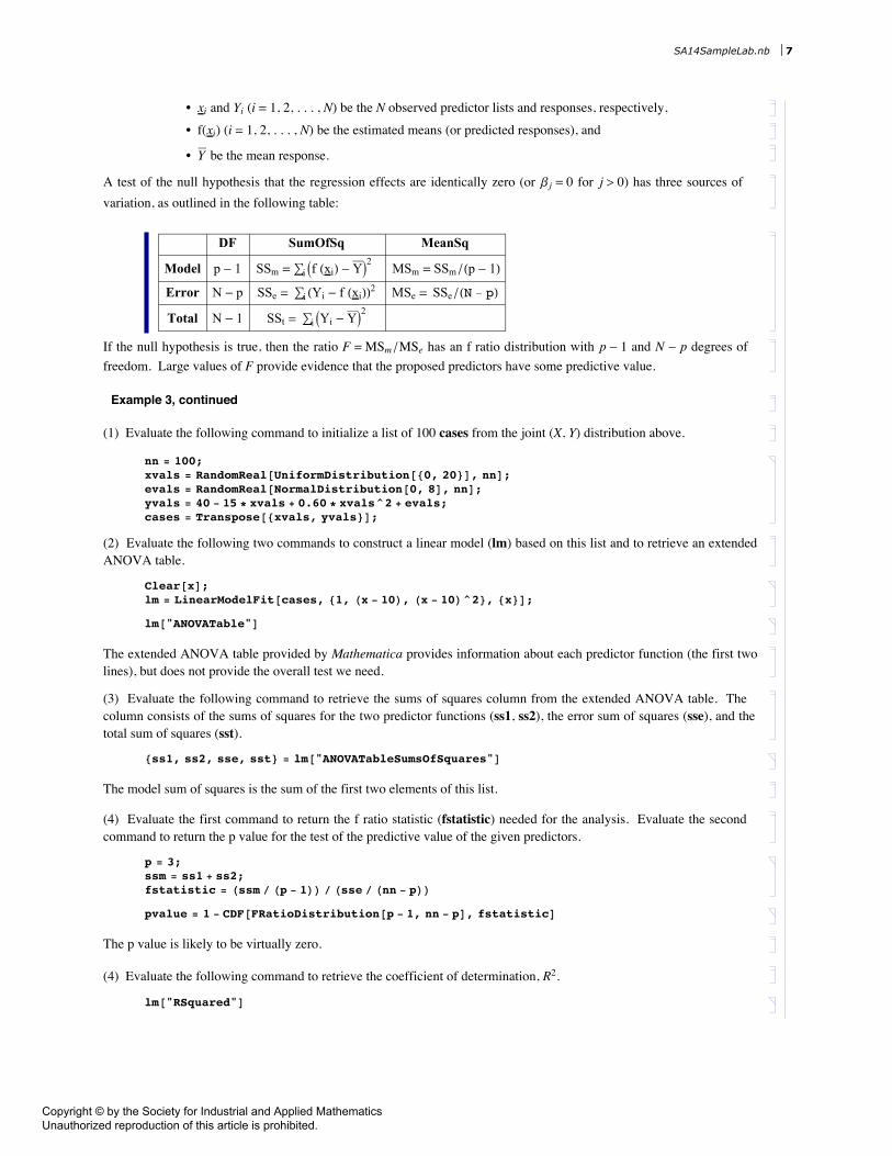
§ 3. Regression Diagnostics
This section focuses on additional methods for interpreting the results of a linear regression analysis. Specifically, scatterplots of
• (estimated mean, estimated error) pairs, and • (case number, estimated standardized influence) pairs
will be constructed using the DiagnosticSummary function.
DiagnosticSummary[lm]returns diagnostic plots of mean-residual pairs and index-delta pairs. Index-delta pairs falling outside the Belsley-Kuh-Welch interval are highlighted in red.
Note that if lm is a fitted model, then lm["PredictedResponse"] returns the list of predicted responses, lm["-FitResiduals"] returns the list of estimated errors, and lm["FitDifferences"] returns the list of estimatedstandardized influences.
Example 5:
To illustrate the plots using simulation, assume that X is a uniform random variable on the interval [0, 80], e is a normalrandom variable with mean 0 and standard deviation 10, and X and e are independent. Let
Y = 2 + 3 X + e .
(1) Evaluate the following command to construct a random sample (pairs) of size 50 from the joint (X, Y) distribution.
nn = 50;xvals = RandomReal@UniformDistribution@80, 80<D, nnD;evals = RandomReal@NormalDistribution@0, 10D, nnD;
yvals = 2 + 3 * xvals + evals;pairs = Transpose@8xvals, yvals<D;
(2) Evaluate the following command to replace the first observed pair with the pair (40, 202) and to construct a scatter-plot of the altered pairs list.
pairs@@1DD = 840, 202<;ScatterPlot@pairs, Correlation Ø TrueD
The plot shows a strong positive association, but there is a point with an unusually large y-coordinate.
(3) Evaluate the first command to construct a fitted linear model (lm) using the adjusted pairs data from above. Evaluatethe second command to construct the diagnostic summary
Clear@xD;lm = LinearModelFit@pairs, 81, x<, 8x<D;
DiagnosticSummary@lmD
The plot on the left compares estimated errors (vertical axis) to estimated means (horizontal axis). The plot on the rightcompares estimated standardized influences (vertical axis) to case numbers (horizontal axis).
Two reports are provided. The first report gives the pairs with the minimum and maximum estimated errors. The errorfor Case 1 is like to be the largest. The second report lists the index-delta pairs whose standardized influence values lieoutside the interval
B-2 p êN , +2 p êN F = @-0.40, +0.40D.
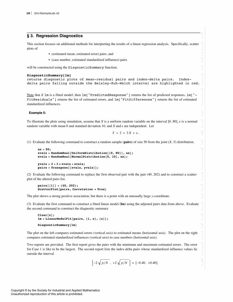
Case 1 is likely to be the only point that is highly influential. That is, the only point whose d value is very far from theinterval @-0.40, +0.40D.
10 SA14SampleLab.nb
Copyright © by the Society for Industrial and Applied Mathematics Unauthorized reproduction of this article is prohibited.
Case 1 is likely to be the only point that is highly influential. That is, the only point whose d value is very far from theinterval @-0.40, +0.40D.
(5) Repeat the simulation several times each using {40, 202} as the first point, and using {40, 42} as the first point, to seedifferent diagnostic plots. To see more unusual plots, try changing the first two points.
Problem 4, continued:(c) Construct and interpret a DiagnosticSummary using the SWS cases data.
Example 6:
The sleep researchers also compared dreaming or paradoxical sleep (PS) in hours to other ecological and environmentalfactors, including the average gestation time (tg) in days for the species and the danger index. They determined that amodel of the form
log10 HPSL = b0 + b1 log10 ItgM + b2 danger + e ,
where e is a normal random variable with mean 0, approximated the data reasonably well.
The lists ps and tgestation give the PS values (in hours) and the tg values (in days) for the 43 species (in alphabeticalorder).
ps, tgestation are lists of length 43.
Click on the rightmost bracket of the cell above and evaluate the command to initialize the data. Re-initialize the data inExamples 2 and 4, if necessary.
Problem 5:(a) Construct a PS cases list where x1corresponds to log10(tg), x2 corresponds to danger, and y corresponds to log10(PS). Use Fit to determine estimates of the b parameters in the formula above. Use PartialPlot to examine the partial regression plots. Comment on the computations.
(b) Repeat Problem 4(a) and 4(c) using the PS cases list.
(c) Use the least squares estimated formula from part (a) to construct five lists of pairs (pairs1 for animals with danger score 1, pairs2 for animals with danger score 2, and so forth) of elements of the form
{x, psx}, x = 20, 80, 140, . . . , 620
where psx is an estimate of the number of hours of PS sleep for a species with average gestation period equal to x days. Construct a scatter plot with the JoinedØTrue option to plot the 5 pairs lists. Comment on the plot.
SA14SampleLab.nb 11
Copyright © by the Society for Industrial and Applied Mathematics Unauthorized reproduction of this article is prohibited.

Part II. Laboratory Examples
Example 1:
X is a uniform random variable on the interval [0, 50], e is a uniform random variable on the interval [|25, 25] and
Y = 2 - 3 X + e .
Students are asked to generate and work with 80 pairs from the joint HX, YL distribution:
nn = 80;xvals = RandomReal@UniformDistribution@80, 50<D, nnD;evals = RandomReal@UniformDistribution@8-25, 25<D, nnD;
yvals = 2 - 3 * xvals + evals;pairs = Transpose@8xvals, yvals<D;
ScatterPlot@pairs, Correlation Ø TrueD
0 10 20 30 40 50 x
-150
-100
-50
0
y
Correlation: -0.9532
Clear@xD; Remove@fD;f@x_D = Fit@pairs, 81, x<, xD
7.37911 - 3.14828 x
Students are asked to repeat the simulations several times each using uniform errors on the intervals
@-25, 25D, @-5, 5D, and @-100, 100D
and to compare the results.
Example 1, continued:
Students are asked to construct an approximate 95% confidence interval for b using 2000 random permutations.
SlopeCI@pairs, RandomPermutations Ø 2000D
8-3.37426, -2.92134<
12 SA14SampleLab.nb
Copyright © by the Society for Industrial and Applied Mathematics Unauthorized reproduction of this article is prohibited.
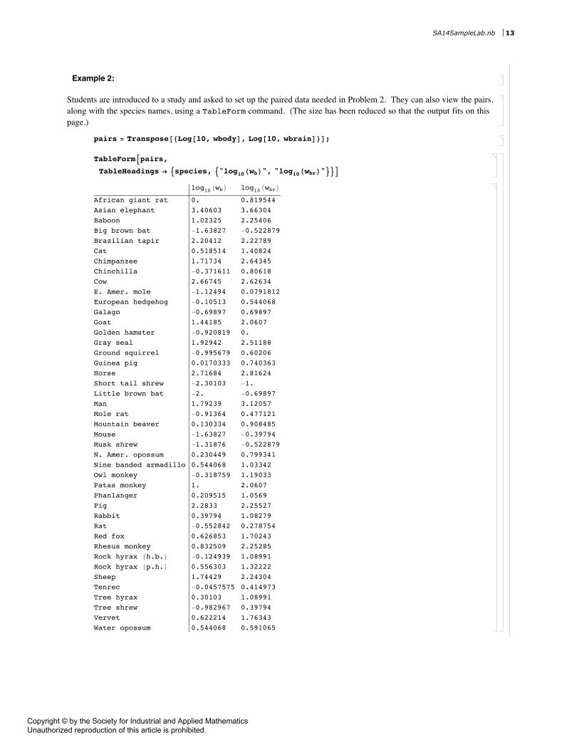
Example 2:
Students are introduced to a study and asked to set up the paired data needed in Problem 2. They can also view the pairs,along with the species names, using a TableForm command. (The size has been reduced so that the output fits on thispage.)
pairs = Transpose@8Log@10, wbodyD, Log@10, wbrainD<D;
TableFormApairs,
TableHeadings Ø 9species, 9"log10HwbL", "log10HwbrL"==E
log10HwbL log10HwbrL
African giant rat 0. 0.819544Asian elephant 3.40603 3.66304Baboon 1.02325 2.25406Big brown bat -1.63827 -0.522879Brazilian tapir 2.20412 2.22789Cat 0.518514 1.40824Chimpanzee 1.71734 2.64345Chinchilla -0.371611 0.80618Cow 2.66745 2.62634E. Amer. mole -1.12494 0.0791812European hedgehog -0.10513 0.544068Galago -0.69897 0.69897Goat 1.44185 2.0607Golden hamster -0.920819 0.Gray seal 1.92942 2.51188Ground squirrel -0.995679 0.60206Guinea pig 0.0170333 0.740363Horse 2.71684 2.81624Short tail shrew -2.30103 -1.Little brown bat -2. -0.69897Man 1.79239 3.12057Mole rat -0.91364 0.477121Mountain beaver 0.130334 0.908485Mouse -1.63827 -0.39794Musk shrew -1.31876 -0.522879N. Amer. opossum 0.230449 0.799341Nine banded armadillo 0.544068 1.03342Owl monkey -0.318759 1.19033Patas monkey 1. 2.0607Phanlanger 0.209515 1.0569Pig 2.2833 2.25527Rabbit 0.39794 1.08279Rat -0.552842 0.278754Red fox 0.626853 1.70243Rhesus monkey 0.832509 2.25285Rock hyrax Hh.b.L -0.124939 1.08991Rock hyrax Hp.h.L 0.556303 1.32222Sheep 1.74429 2.24304Tenrec -0.0457575 0.414973Tree hyrax 0.30103 1.08991Tree shrew -0.982967 0.39794Vervet 0.622214 1.76343Water opossum 0.544068 0.591065
SA14SampleLab.nb 13
Copyright © by the Society for Industrial and Applied Mathematics Unauthorized reproduction of this article is prohibited.

Example 3:
X is a uniform random variable on the interval [0, 20], e is a normal random variable with mean m = 0 and s = 8, X and eare independent, and
Y = 40 - 15 X + 0.60 X2 + e = -50 - 3 HX - 10L + 0.60 HX - 10L2 + e.
Students are asked to generate and work with 100 cases from the joint (X, Y) distribution.
nn = 100;xvals = RandomReal@UniformDistribution@80, 20<D, nnD;evals = RandomReal@NormalDistribution@0, 8D, nnD;yvals = 40 - 15 * xvals + 0.60 * xvals^2 + evals;cases = Transpose@8xvals, yvals<D;
Clear@xD; Remove@fD;f@x_D = Fit@cases, 81, x - 10, Hx - 10L^2<, xD
-51.3511 - 3.00928 H-10 + xL + 0.606323 H-10 + xL2
SmoothPlot@8cases, f<D
0 5 10 15 20 x-80
-60
-40
-20
0
20
40
60y
Example 3, continued
The 100 cases from the joint (X, Y) distribution above can be analyzed using LinearModelFit.
Clear@xD;lm = LinearModelFit@cases, 81, Hx - 10L, Hx - 10L^2<, 8x<D;
lm@"ANOVATable"D
DF SS MS F Statistic P-Value
-10 + x 1 20853.8 20853.8 380.359 2.45509µ10-35
H-10 + xL2 1 31754. 31754. 579.173 1.0989µ10-42
Error 97 5318.16 54.8264Total 99 57925.9
8ss1, ss2, sse, sst< = lm@"ANOVATableSumsOfSquares"D;p = 3;ssm = ss1 + ss2;fstatistic = Hssm ê Hp - 1LL ê Hsse ê Hnn - pLL
479.766
pvalue = 1 - CDF@FRatioDistribution@p - 1, nn - pD, fstatisticD
0.
14 SA14SampleLab.nb
Copyright © by the Society for Industrial and Applied Mathematics Unauthorized reproduction of this article is prohibited.
lm@"RSquared"D
0.90819
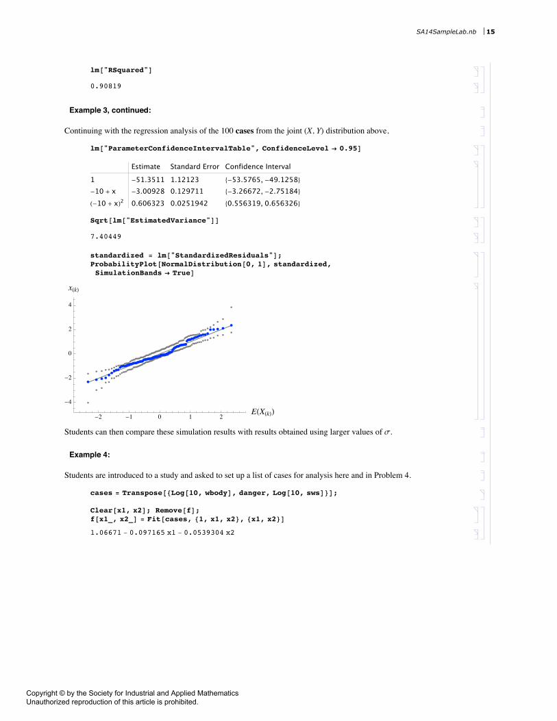
Example 3, continued:
Continuing with the regression analysis of the 100 cases from the joint (X, Y) distribution above,
lm@"ParameterConfidenceIntervalTable", ConfidenceLevel Ø 0.95D
Estimate Standard Error Confidence Interval
1 -51.3511 1.12123 8-53.5765, -49.1258<-10 + x -3.00928 0.129711 8-3.26672, -2.75184<H-10 + xL2 0.606323 0.0251942 80.556319, 0.656326<
Sqrt@lm@"EstimatedVariance"DD
7.40449
standardized = lm@"StandardizedResiduals"D;ProbabilityPlot@NormalDistribution@0, 1D, standardized,SimulationBands Ø TrueD
-2 -1 0 1 2EHXHkLL
-4
-2
0
2
4
xHkL
Students can then compare these simulation results with results obtained using larger values of s.
Example 4:
Students are introduced to a study and asked to set up a list of cases for analysis here and in Problem 4.
cases = Transpose@8Log@10, wbodyD, danger, Log@10, swsD<D;
Clear@x1, x2D; Remove@fD;f@x1_, x2_D = Fit@cases, 81, x1, x2<, 8x1, x2<D
1.06671 - 0.097165 x1 - 0.0539304 x2
SA14SampleLab.nb 15
Copyright © by the Society for Industrial and Applied Mathematics Unauthorized reproduction of this article is prohibited.

PartialPlot@cases, 1D
-3 -2 -1 1 2 3 x
-0.4
-0.2
0.2
y
Equation of Line: y = -0.097165x
Students construct a partial regression plot for the second predictor as well.
Example 5:
X is a uniform random variable on the interval [0, 80], e is a normal random variable with mean m = 0 and s = 10, X and eare independent, and
Y = 2 + 3 X + e .
Students construct 50 random pairs and change the first pair. A DiagnosticSummary of the fitted linear modelidentifies the changed point as highly influential.
nn = 50;xvals = RandomReal@UniformDistribution@80, 80<D, nnD;evals = RandomReal@NormalDistribution@0, 10D, nnD;
yvals = 2 + 3 * xvals + evals;pairs = Transpose@8xvals, yvals<D;
pairs@@1DD = 840, 202<;ScatterPlot@pairs, Correlation Ø TrueD
0 20 40 60 80 x0
50
100
150
200
250
y
Correlation: 0.9791
16 SA14SampleLab.nb
Copyright © by the Society for Industrial and Applied Mathematics Unauthorized reproduction of this article is prohibited.
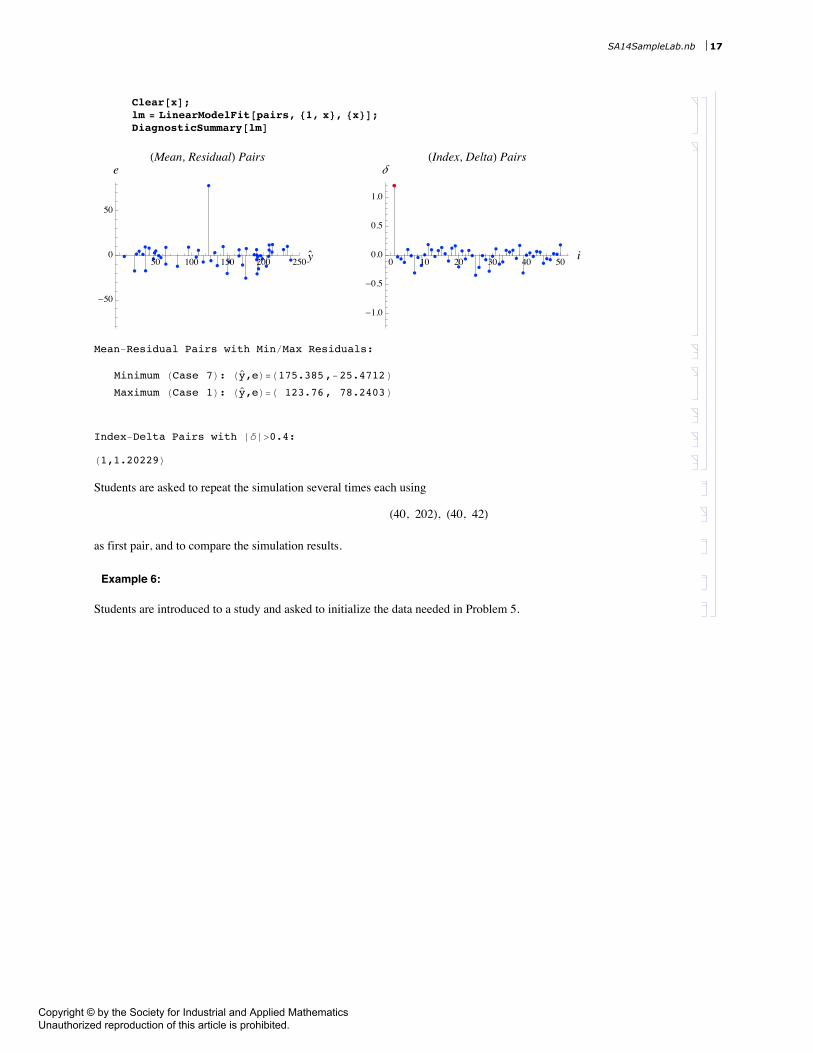
Clear@xD;lm = LinearModelFit@pairs, 81, x<, 8x<D;DiagnosticSummary@lmD
50 100 150 200 250y`
-50
0
50
eHMean, ResidualL Pairs
0 10 20 30 40 50 i
-1.0
-0.5
0.0
0.5
1.0
dHIndex, DeltaL Pairs
Mean-Residual Pairs with MinêMax Residuals:
Minimum HCase 7L: Hy`,eL=H175.385,-25.4712L
Maximum HCase 1L: Hy`,eL=H 123.76, 78.2403L
Index-Delta Pairs with »d»>0.4:
H1,1.20229L
Students are asked to repeat the simulation several times each using
H40, 202L, H40, 42L
as first pair, and to compare the simulation results.
Example 6:
Students are introduced to a study and asked to initialize the data needed in Problem 5.
SA14SampleLab.nb 17
Copyright © by the Society for Industrial and Applied Mathematics Unauthorized reproduction of this article is prohibited.

Part III. Laboratory 14 Solutions
Problem 1: Y = 2 - 3 X + e where X is uniform on [0,80] and e is uniform on [|50,50].
(a) Analyses based on 100 simulated pairs:
nn = 100;xvals = RandomReal@UniformDistribution@80, 80<D, nnD;evals = RandomReal@UniformDistribution@8-50, 50<D, nnD;yvals = 2 - 3 * xvals + evals;pairs = Transpose@8xvals, yvals<D;
Sample summaries for the X and Y samples are as follows:
8mx, sdx< = 8Mean@xvalsD, StandardDeviation@xvalsD<
840.57, 22.8826<
8my, sdy< = 8Mean@yvalsD, StandardDeviation@yvalsD<
8-118.334, 74.7375<
A scatter plot of pairs and the least squares formula for the conditional mean are shown below:
ScatterPlot@pairs, Correlation Ø TrueD
0 20 40 60 80 x
-250
-200
-150
-100
-50
0
50y
Correlation: -0.9205
Clear@xD; Remove@fDf@x_D = Fit@pairs, 81, x<, xD
3.6413 - 3.00654 x
The approximate 95% permutation confidence interval (shown below) contains |3.
SlopeCI@pairs, RandomPermutations Ø 2000D
8-3.26915, -2.74907<
(b) Model summaries:
model1 = UniformDistribution@80, 80<D;model2 = UniformDistribution@8-50, 50<D;
(1) The mean and standard deviation of X are as follows:
8mx, sx< = N@8Mean@model1D, StandardDeviation@model1D<D
840., 23.094<
(2) The mean and standard deviation of Y = 2 - 3 X + e are
18 SA14SampleLab.nb
Copyright © by the Society for Industrial and Applied Mathematics Unauthorized reproduction of this article is prohibited.

(2) The mean and standard deviation of Y = 2 - 3 X + e are
E HYL = 2 - 3 E HXL + E HeL = -118 and SD HYL = 9 Var HXL + Var HeL º 75.06
as demonstrated below:
my = 2 - 3 * Mean@model1D + Mean@model2D
-118
sy = N@Sqrt@9 * Variance@model1D + Variance@model2DDD
75.0555
(3) To compute the correlation, first note that
Cov HX, YL = Cov HX, 2 - 3 X + eL = -3 Var HXL.
Thus, the correlation is as follows:
r = H-3 Variance@model1DL ê Hsx * syL
-0.923077
(4) Comparison of estimates with model values:
8mx, sdx, my, sdy, Correlation@xvals, yvalsD<
840.57, 22.8826, -118.334, 74.7375, -0.92052<
8mx, sx, my, sy, r<
840., 23.094, -118, 75.0555, -0.923077<
In each case, the estimate is close to the model summary.
Problem 2: Analysis of brain-body data.
species, wbody, wbrain are lists of length 43.
(a) The least squares linear fit formula, and approximate 95% confidence interval for the slope are shown below:
pairs = Transpose@8Log@10, wbodyD, Log@10, wbrainD<D;Clear@xD; Remove@fD;f@x_D = Fit@pairs, 81, x<, xD
0.930348 + 0.782263 x
SlopeCI@pairs, RandomPermutations Ø 2000D
80.70797, 0.859893<
Since the 95% confidence interval does not contain zero, there is a significant regression effect.
Since slope corresponds to the rate of change of y with respect to a unit change in x and we are working on the log scale,the interpretation is as follows: If average body weight increases by a factor of 10, then average brain weight willincrease by a factor of about 6.06, as demonstrated below.
10^0.782263
6.05708
(b) The gorilla's predicted response is 2.74205 log-grams (552.136 grams).
SA14SampleLab.nb 19
Copyright © by the Society for Industrial and Applied Mathematics Unauthorized reproduction of this article is prohibited.

(b) The gorilla's predicted response is 2.74205 log-grams (552.136 grams).
lwb = Log@10, 207.0D;8f@lwbD, 10^f@lwbD<
82.74205, 552.136<
The actual response is 2.60853 log-grams (406 grams), as demonstrated below:
lwbr = Log@10, 406.0D
2.60853
The following computation demonstrates that the predicted response is about 5.1% larger than the actual value.
Hf@lwbD - lwbrL ê lwbr
0.0511859
Thus, the values are reasonably close on the log-scale. On the original scale, however, the values are not very close (theerror is approximately 36% of the actual value).
(c) The definition of g and smoothed scatter plot are shown below.
Clear@xD; Remove@gD;g@x_D = Simplify@10^f@Log@10, xDDD
8.51821 x0.782263
pairs2 = Transpose@8wbody, wbrain<D;SmoothPlot@8pairs2, g<,AxesLabel Ø 8"wb", "wbr"<D
0 500 1000 1500 2000 2500wb
0
1000
2000
3000
4000
5000wbr
Average brain weight increases as body weight increases, although the rate of increase decreases with body weight.Body and brain weights for the Asian elephant are very different from those of other species considered in this problem.
20 SA14SampleLab.nb
Copyright © by the Society for Industrial and Applied Mathematics Unauthorized reproduction of this article is prohibited.

Problem 3: X is a uniform random variable on the interval [0,20].
(1) The correlation between X and X2 is approximately 0.97, as demonstrated below:
• Mean and standard deviation of X :
model = UniformDistribution@80, 20<D;8m1, s1< = 8Mean@modelD, StandardDeviation@modelD<
:10,10
3>
• Mean and standard deviation of X2:
m2 = Integrate@x^2 ê 20, 8x, 0, 20<D
400
3
s2 = Sqrt@Integrate@Hx^2 - m2L^2 ê 20, 8x, 0, 20<DD
160 5
3
• Covariance between X and X2:
s12 = Integrate@x^3 ê 20, 8x, 0, 20<D - m1 * m2
2000
3
• Correlation between X and X2:
N@s12 ê Hs1 * s2LD
0.968246
(2) Since
Cov IX - 10, HX - 10L2M = Cov IX - 10, X2 - 20 X + 100M = Cov IX, X2M - 20 Var HXL = 0
s12 - 20 s1^2
0
the correlation between X|10 and HX|10L2is also zero.
Problem 4: Analysis of the SWS cases data.
danger, sws are lists of length 43.
cases = Transpose@8Log@10, wbodyD, danger, Log@10, swsD<D;nn = Length@casesD;Clear@x1, x2D; Remove@fD;f@x1_, x2_D = Fit@cases, 81, x1, x2<, 8x1, x2<D
1.06671 - 0.097165 x1 - 0.0539304 x2
(a) Regression analysis of the SWS cases list:
SA14SampleLab.nb 21
Copyright © by the Society for Industrial and Applied Mathematics Unauthorized reproduction of this article is prohibited.
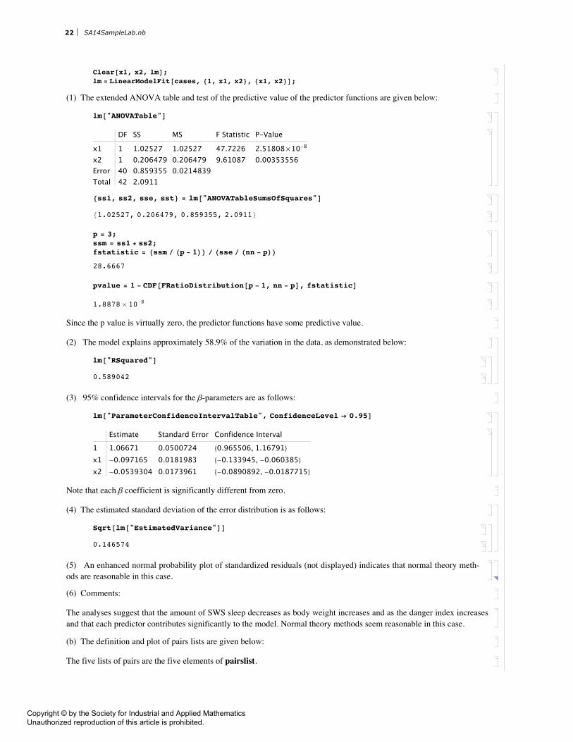
Clear@x1, x2, lmD;lm = LinearModelFit@cases, 81, x1, x2<, 8x1, x2<D;
(1) The extended ANOVA table and test of the predictive value of the predictor functions are given below:
lm@"ANOVATable"D
DF SS MS F Statistic P-Value
x1 1 1.02527 1.02527 47.7226 2.51808µ10-8
x2 1 0.206479 0.206479 9.61087 0.00353556Error 40 0.859355 0.0214839Total 42 2.0911
8ss1, ss2, sse, sst< = lm@"ANOVATableSumsOfSquares"D
81.02527, 0.206479, 0.859355, 2.0911<
p = 3;ssm = ss1 + ss2;fstatistic = Hssm ê Hp - 1LL ê Hsse ê Hnn - pLL
28.6667
pvalue = 1 - CDF@FRatioDistribution@p - 1, nn - pD, fstatisticD
1.8878 µ 10-8
Since the p value is virtually zero, the predictor functions have some predictive value.
(2) The model explains approximately 58.9% of the variation in the data, as demonstrated below:
lm@"RSquared"D
0.589042
(3) 95% confidence intervals for the b-parameters are as follows:
lm@"ParameterConfidenceIntervalTable", ConfidenceLevel Ø 0.95D
Estimate Standard Error Confidence Interval
1 1.06671 0.0500724 80.965506, 1.16791<x1 -0.097165 0.0181983 8-0.133945, -0.060385<x2 -0.0539304 0.0173961 8-0.0890892, -0.0187715<
Note that each b coefficient is significantly different from zero.
(4) The estimated standard deviation of the error distribution is as follows:
Sqrt@lm@"EstimatedVariance"DD
0.146574
(5) An enhanced normal probability plot of standardized residuals (not displayed) indicates that normal theory meth-ods are reasonable in this case.
(6) Comments:
The analyses suggest that the amount of SWS sleep decreases as body weight increases and as the danger index increasesand that each predictor contributes significantly to the model. Normal theory methods seem reasonable in this case.
(b) The definition and plot of pairs lists are given below:
The five lists of pairs are the five elements of pairslist.
22 SA14SampleLab.nb
Copyright © by the Society for Industrial and Applied Mathematics Unauthorized reproduction of this article is prohibited.

pairslist = Table@Table@8x, 10^f@x, jD<, 8x, -1, 3<D, 8j, 1, 5<D;
ScatterPlotApairslist,Joined Ø True,AxesLabel Ø 9"log10HwbL", "SWS"=,
ChartLegends Ø 8"Danger 1", "Danger 2", "Danger 3", "Danger 4", "Danger 5"<E
-1 0 1 2 3log10HwbL
4
6
8
10
12
SWS
Danger 1Danger 2Danger 3Danger 4Danger 5
The plot suggests that the amount of SWS sleep decreases with increasing body weight and with increasing danger index.
(c) The diagnostic summary plot is given below.
DiagnosticSummary@lmD
0.6 0.7 0.8 0.9 1.0 1.1 1.2 y`
-0.3
-0.2
-0.1
0.0
0.1
0.2
0.3
eHMean, ResidualL Pairs
0 10 20 30 40 i
-0.6
-0.4
-0.2
0.0
0.2
0.4
0.6
dHIndex, DeltaL Pairs
Mean-Residual Pairs with MinêMax Residuals:
Minimum HCase 10L: Hy`,eL=H1.12208,-0.32274L
Maximum HCase 29L: Hy`,eL=H0.75382, 0.24618L
Index-Delta Pairs with »d»>0.528271:
H2,-0.630684L H10,-0.658695L H18,-0.605661LH19,-0.699289L
From the mean-residual pairs plot, we see that there is no apparent relationship between residuals and predictedresponses.
Although 4 species have d values outside the interval [|0.528, +0.528], none of the values are very far from the interval.Note that in each case, the observed response was less than the predicted response.
SA14SampleLab.nb 23
Copyright © by the Society for Industrial and Applied Mathematics Unauthorized reproduction of this article is prohibited.

Problem 5: Analysis of PS cases data.
ps, tgestation are lists of length 43.
(a) Initial analyses of the PS cases data:
cases = Transpose@8Log@10, tgestationD, danger, Log@10, psD<D;nn = Length@casesD;Clear@x1, x2D; Remove@fDf@x1_, x2_D = Fit@cases, 81, x1, x2<, 8x1, x2<D
1.06246 - 0.300001 x1 - 0.108528 x2
Partial plots (not shown) indicate that adjusted log-PS values are negatively associated with adjusted xi values. In eachcase, there was one point (the Asian elephant) with an unusually high y-coordinate.
(b) Regression analyses of the PS cases data:
Clear@x1, x2, lmD;lm = LinearModelFit@cases, 81, x1, x2<, 8x1, x2<D;
(1) The extended ANOVA table and test of the predictive value of the predictor functions are given below:
lm@"ANOVATable"D
DF SS MS F Statistic P-Value
x1 1 1.43394 1.43394 45.6721 4.07898µ10-8
x2 1 0.86259 0.86259 27.4741 5.46741µ10-6
Error 40 1.25586 0.0313965Total 42 3.55239
8ss1, ss2, sse, sst< = lm@"ANOVATableSumsOfSquares"D
81.43394, 0.86259, 1.25586, 3.55239<
p = 3;ssm = ss1 + ss2;fstatistic = Hssm ê Hp - 1LL ê Hsse ê Hnn - pLL
36.5731
pvalue = 1 - CDF@FRatioDistribution@p - 1, nn - pD, fstatisticD
9.29817 µ 10-10
Since the p value is virtually zero, the predictors have some predictive value.
(2) The model explains approximately 64.6% of the variation in the data, as demonstrated below:
lm@"RSquared"D
0.646475
(3) 95% confidence intervals for the b parameters are as follows:
lm@"ParameterConfidenceIntervalTable", ConfidenceLevel Ø 0.95D
Estimate Standard Error Confidence Interval
1 1.06246 0.118072 80.823826, 1.30109<x1 -0.300001 0.0632294 8-0.427792, -0.17221<x2 -0.108528 0.0207053 8-0.150375, -0.0666814<
Each b coefficient is significantly different from zero.
24 SA14SampleLab.nb
Copyright © by the Society for Industrial and Applied Mathematics Unauthorized reproduction of this article is prohibited.

Each b coefficient is significantly different from zero.
(4) The estimated standard deviation of the error distribution is as follows:
Sqrt@lm@"EstimatedVariance"DD
0.177191
(5) An enhanced normal probability plot (not shown) suggests that normal theory methods are reasonable in this case.
(6) Comments:
The analyses suggest that the amount of PS sleep decreases as the average gestational time and danger indices increaseand that each predictor contributes significantly to the model. Normal theory methods seem reasonable in this case.
(7) Diagnostic summary:
DiagnosticSummary@lmD
-0.2 0.0 0.2 0.4 0.6 y`
-0.4
-0.2
0.0
0.2
0.4
eHMean, ResidualL Pairs
10 20 30 40 i
-1.0
-0.5
0.0
0.5
1.0
dHIndex, DeltaL Pairs
Mean-Residual Pairs with MinêMax Residuals:
Minimum HCase 40L: Hy`,eL=H0.0465621,-0.347592L
Maximum HCase 2L: Hy`,eL=H-0.210213, 0.465486L
Index-Delta Pairs with »d»>0.528271:
H2,1.13166L
The mean-residual pairs plot shows no apparent relationship between estimated means and standardized residuals. Note,however, that there is one large outlier, corresponding to the Asian elephant.
species@@2DD
Asian elephant
The standardized influence for the Asian elephant (1.132) is unusually high.
(c) The definition and plot of pairs lists are given below:
The five lists of pairs are the five elements of pairslist.
SA14SampleLab.nb 25
Copyright © by the Society for Industrial and Applied Mathematics Unauthorized reproduction of this article is prohibited.
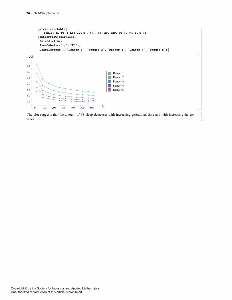
pairslist = Table@Table@8x, 10^f@Log@10, xD, jD<, 8x, 20, 620, 60<D, 8j, 1, 5<D;
ScatterPlotApairslist,Joined Ø True,AxesLabel Ø 9"tg", "PS"=,
ChartLegends Ø 8"Danger 1", "Danger 2", "Danger 3", "Danger 4", "Danger 5"<E
0 100 200 300 400 500 600tg
0.5
1.0
1.5
2.0
2.5
3.0
3.5
PS
Danger 1Danger 2Danger 3Danger 4Danger 5
The plot suggests that the amount of PS sleep decreases with increasing gestational time and with increasing dangerindex.
26 SA14SampleLab.nb
Copyright © by the Society for Industrial and Applied Mathematics Unauthorized reproduction of this article is prohibited.
Related Documents


![Mathematica - portal.tpu.ru · 9 Mathematica ˜ , Sin[x]. Mathematica ˙˝ - . 2 . ˚˙ * 2 Mathematica Pi , % = 3.14159… E , e = 2.71828… I Infinity ˝˙˝" , ˛˝ ˇ"ˆ](https://static.cupdf.com/doc/110x72/5eacdd5613bbdc7d5c10b806/mathematica-9-mathematica-oe-sinx-mathematica-2-2-mathematica.jpg)