Math 245, Fall 2010

Compact course notes

Math 245, Fall 2010Linear Algebra 2

Professor: S. Newtranscribed by: J. Lazovskis

University of WaterlooDecember 17, 2010

Contents

1 Overview of Linear Algebra 1 21.1 Lines and planes . . . . . . . . . . . . . . . . . . . . . . . . . . . . . . . . . . . . . . . . . . . 21.2 Determinants . . . . . . . . . . . . . . . . . . . . . . . . . . . . . . . . . . . . . . . . . . . . . 3

2 Operations in vector spaces 32.1 The dot product in Rn . . . . . . . . . . . . . . . . . . . . . . . . . . . . . . . . . . . . . . . . 32.2 Orthogonal projections . . . . . . . . . . . . . . . . . . . . . . . . . . . . . . . . . . . . . . . . 42.3 The cross product in Rn . . . . . . . . . . . . . . . . . . . . . . . . . . . . . . . . . . . . . . . 5

3 Applications of the cross product 63.1 Geometry . . . . . . . . . . . . . . . . . . . . . . . . . . . . . . . . . . . . . . . . . . . . . . . 63.2 Spherical geometry . . . . . . . . . . . . . . . . . . . . . . . . . . . . . . . . . . . . . . . . . . 63.3 Spherical angles . . . . . . . . . . . . . . . . . . . . . . . . . . . . . . . . . . . . . . . . . . . . 7

4 The inner product 84.1 Fundamental definitions . . . . . . . . . . . . . . . . . . . . . . . . . . . . . . . . . . . . . . . 84.2 Standard inner products . . . . . . . . . . . . . . . . . . . . . . . . . . . . . . . . . . . . . . . 84.3 Orthogonal sets / compliments / projections . . . . . . . . . . . . . . . . . . . . . . . . . . . . 94.4 Quotient spaces . . . . . . . . . . . . . . . . . . . . . . . . . . . . . . . . . . . . . . . . . . . . 104.5 Dual spaces . . . . . . . . . . . . . . . . . . . . . . . . . . . . . . . . . . . . . . . . . . . . . . 114.6 Normal linear maps, etc . . . . . . . . . . . . . . . . . . . . . . . . . . . . . . . . . . . . . . . 12

5 Bilinear and quadratic forms 135.1 Bilinear forms . . . . . . . . . . . . . . . . . . . . . . . . . . . . . . . . . . . . . . . . . . . . . 135.2 Quadratic forms . . . . . . . . . . . . . . . . . . . . . . . . . . . . . . . . . . . . . . . . . . . 155.3 Characterization and extreme values . . . . . . . . . . . . . . . . . . . . . . . . . . . . . . . . 15

6 Jordan normal form 166.1 Block form . . . . . . . . . . . . . . . . . . . . . . . . . . . . . . . . . . . . . . . . . . . . . . 166.2 Canonical form . . . . . . . . . . . . . . . . . . . . . . . . . . . . . . . . . . . . . . . . . . . . 16

7 Selected proofs 18

1

1 Overview of Linear Algebra 1

1.1 Lines and planes

A line in 3 dimensions is best described parametrically. Given a point p and a vector u, all points on theline are described by x = p+ tu for t ∈ R.

A plane in 3 dimensions is the same; given two points and two vectors p+ u and q + v, the points on theplane are described by x = p+ ru+ st for s, r ∈ R. This can be generalized by a1x1 + a2x2 + a3x3 = b.

Definition 1.1.1. A vector space in Rn is a set of the form {t1u1, . . . , tkuk|ti ∈ R} = span{u1, . . . , uk ∈ R}.Avector space includes the origin.

Definition 1.1.2. An affine space in Rn is a set of the form p+ V = {p+ v|v ∈ V }, for some point p ∈ Rnand some vector space V ∈ Rn. Here, p+ V is the affine space through p parallel to V .

Theorem 1.1.3. If U is a basis for a vector space V ∈ Rn, then the number of elements in U is at most n.If U and W are bases for the same vector space in Rn, then they have the same number of elements. Thisnumber is termed dimension.

Definition 1.1.4. A function A is said to be linear if the two following conditions are satisfied for somescalar t and all x, y ∈ Rn:A(tx) = tA(x)A(x+ y) = A(x) +A(y)

Definition 1.1.5. A linear map L : Rn → Rm is a map of the form L(x) = Ax for some A ∈Mm×n.

Definition 1.1.6. An affine map L : Rn → Rm is a map of the form L(x) = Ax+ b for some A ∈Mm×nand b ∈ Rn.

· Note that the span of columns is the column space of the range.

· The nullspace is perpendicular to the rowspace.

Theorem 1.1.7. Suppose that L : Rn → Rn is linear. Let x ∈ Rn be such that x = x1e1 + x2e2 + · · ·+ xnen,where ek is the kth standard basis vector. Then L(x) = Ax for A = (L(e1) L(e2) . . . L(en)).

Theorem 1.1.8. Suppose A reduces to R in reduced row echelon form. Then the non-zero rows of R form abasis for the row space of A. Then to obtain a basis for the nullspace of A, solve Ax = 0 using Gauss-Jordanelimination to get x = t1v1 + · · ·+ tkvkthen {u1, . . . , uk} is a basis for null(A).

Definition 1.1.9. Given a function f : X → Y :1. f is 1:1 or injective when for all y ∈ Y there exists at most 1 x ∈ X such that y = f(x).2. f is onto or surjective when for all y ∈ Y there exists at least 1 x ∈ X such that y = f(x).3. f is invertible or bijective when f is one-to-one and onto.

Theorem 1.1.10. A function is differentiable when it can be suitably approximated by an affine map.

Definition 1.1.11. Let U and V be vector spaces with dim(U) = n and dim(V ) = n. Let U = {u1, . . . , un}and V = {v1, . . . , vn} be ordered bases for for U and V respectively. Then for x ∈ U with x = t1u1 + · · ·+ tnun,

define [x]U = t =

t1...tn

∈ Rn

For a linear map L : U → V , there is a unique matrix described by [L]UV such that for all x ∈ U ,

[L(x)]V = [L]UV [x]U . This matrix is given by [L]UV =([L(u1)]V . . . [L(un)]V

)∈Mm×n

Remark 1.1.12. The matrix [L]UV is termed the matrix of L with respect to the bases U and V.

2

1.2 Determinants

Theorem 1.2.1. Given matrices A,B ∈Mn×n and an equation AB = 0,(A|ei) ∼ (I|Bi)(A|I) ∼ (I|B)

where ei is the ith column of I and Bi is the ith column of B.

Definition 1.2.2. For n > 2 and A ∈Mn×n, given a fixed i, det(A) =

n∑j=1

(−1)i+jAi,jdet(Ai,j)

· where Ai,j is the (n− 1)× (n− 1) matrix obtained from A by removing the ith row and jth column· and Ai,j is the element in the ith row and jth column of A

Theorem 1.2.3. If Null(A) 6= {0}, then A is not invertible and det(A) = 0.

Definition 1.2.4. The matrix defined by Cofac(A) is termed the cofactor matrix (or classical adjoint)of A.

Theorem 1.2.5. ForA ∈Mm×n, A is invertible if and only if det(A) 6= 0, and in that caseA−1 = 1det(A) · Cofac(A)

where (Cofac(A))k,` = (−1)k+`det(A`,k)

Theorem 1.2.6. For all A ∈Mn×n, A · Cofac(A) = det(A)I. Also, Cofac(A) = (Aadj)t.

Theorem 1.2.7. [Inversion properties]For any A,B ∈Mn×n, det(AB) = det(A) det(B)For any A ∈Mn×n and for t ∈ N, det(A) = det(At)

2 Operations in vector spaces

Remark 2.0.1. A vector space over a field F is a set closed over addition and multiplication.

Remark 2.0.2. Let U, V be finite dimensional vector spaces with bases U1,U2,V1,V2. For any u ∈ U andlinear map L : U → V ,

[u]U2 = [I]U1U2 [u]U1 [L]U2V2 = [I]V1V2 [L]U1V1 [I]U2U1

Definition 2.0.3. For A,B ∈Mn×n, A and B are similar when there exists an invertible matrix P suchthat B = PAP−1.

2.1 The dot product in Rn

Definition 2.1.1. For u, v ∈ Rn, the dot product of u and v is u · v =

n∑i=1

u1v1 = utv = vtu.

Theorem 2.1.2. [Properties of the dot product]For t ∈ R and u, v, w ∈ Rn:

1. u · u > 0 with u · u = 0⇐⇒ u = 0 Positive definite2. u · v = v · u Symmetric3. (tu) · v = t(u · v) = u · (tv) Bilinear4. (u+ w) · w = u · w + v · w

Remark 2.1.3. For any A ∈Mm×n and x ∈ Rn, we have Ax = (c1 . . . cn)

x1...xn

= c1x1 + · · ·+ cnxn.

Also note that the row space of A is equal to the column space of A.

Definition 2.1.4. For u ∈ Rn, the length of u is

√√√√ n∑i=1

u2i =√u · u = |u|.

3

Theorem 2.1.5. [Properties of length]For u, v ∈ Rn and t ∈ R,

1. |u| > 0 with |u| = 0 ⇐⇒ u = 02. |tu| = |t| |u|3. u · v = 1

2 (|u+ v|2 − |u|2 − |v|2) = 14 (|u+ v|2 − |u− v|2)

4. |u · v| 6 |u||v| with |u · v| = |u||v| ⇐⇒ {u, v} is linearly dependent5. |u− v| 6 |u+ v| 6 |u|+ |v|

Definition 2.1.6. For u, v ∈ Rn, the distance between u and v is d(u, v) = |u− v| = |v − u|.

Theorem 2.1.7. [Properties of distance]For u, v, w ∈ Rn,

1. d(u, v) > 0 with d(u, v) = 0 ⇐⇒ u = v2. d(u, v) = d(v, u)3. d(u, v) 6 d(u,w) + d(w, v)

Definition 2.1.8. For 0 6= u, v ∈ Rn, the angle between u and v is angle(u, v) = θ. This is expressed as

θ = cos−1(u · v|u||v|

)= sin−1

(|u× v||u||v|

).

Theorem 2.1.9. [Properties of angles]For 0 6= u, v ∈ Rn and θ = angle(u, v):

1. Law of cosines: |v − u|2 = |u|2 + |v|2 − 2|u||v| cos(θ)2. Pythagorean theorem: If u · (v − u) = 0, then |v|2 = |u|2 + |v − u|2

3. Trigonometric ratios: If u · (v − u) = 0, then cos(θ) = |u||v| and sin(θ) = |v−u|

|v|

Theorem 2.1.10. For t ∈ R and u, v ∈ Rn and t, u, v 6= 0:

angle(tu, v) =

{angle(u, v) if t > 0π − angle(u, v) if t < 0

Definition 2.1.11. For a, b, c ∈ Rn all distinct, define ∠abc = angle(a− b, c− b).

Theorem 2.1.12. For a, b, c ∈ Rn all distinct, ∠abc+ ∠cab+ ∠bca = π.

Definition 2.1.13. For 0 6= u ∈ Rn and p ∈ Rn, the hyperspace (or hyperplane) in Rn through p andperpendicular to u is the set of points x ∈ Rn such that (x− p) · u = 0.

2.2 Orthogonal projections

Definition 2.2.1. For u, v ∈ Rn, we say that u and v are orthogonal (or perpendicular) when u · v = 0.If u, v 6= 0, then u · v = 0 ⇐⇒ angle(u, v) = π

2 .

Definition 2.2.2. For 0 6= u ∈ Rn and x ∈ Rn, the orthogonal projection of x onto u is proju(x) = u·x|u| .

If U = span{u}, then projU (x) = u·x|u|2u. Note that (x− proju(x)) is orthogonal to u.

With reference to the case above, [projUx] = 1|u|2uu

t.

Definition 2.2.3. For a vector space U ∈ Rn, the orthogonal complement of U is the vector space

U⊥ = {x ∈ Rn|x · u = 0 for all u ∈ U} = Null(U t).

The projection of x onto U⊥ is x− projUx.

Theorem 2.2.4. [Properties of the orthogonal complement]Let U be a vector space in Rn. Then

1. For A ∈Mm×n over R, Null(A) = Row(A)⊥

2. U ∩ U⊥ = {0}3. dim(U)+ dim(U⊥) = n4. (U⊥)⊥ = U

4

Theorem 2.2.5. For A ∈Mm×n, rank(AtA) = rank(A). Also, Null(AtA) = Null(A).

Theorem 2.2.6. Let U be a vector space in Rn and x ∈ Rn. Then there exist unique vectors u, v ∈ Rn withu ∈ U and v ∈ U⊥ such that u+ v = x.

Corollary 2.2.7. When {u1, . . . , uk} is a basis for U and A = (u1 . . . uk) ∈Mn×k, then· ProjU (x) = A(AtA)−1Atx· ProjU⊥(x) = (I −A(AtA)−1At)x.

Definition 2.2.8. Let U be a subspace of Rn and let x ∈ Rn. Let u, v be the unique vectors with u ∈ U andv ∈ U⊥ with u+ v = x. Then u is termed the orthogonal projection of x onto U and we write u = ProjU (x).

Note that since (U⊥)⊥ = U , we have v = ProjU⊥(x).

Theorem 2.2.9. Let U be a subspace of Rn with x ∈ Rn. Then the point u = ProjU (x) is the unique pointon U which is nearest to x.

Theorem 2.2.10. Given a set of data points {(x1, y1), (x2, y2), . . . , (xn, yn)}, the polynomial f ∈ Pmwith f(x) = c0 + c1x+ c2x

2 + · · ·+ cmxm that best fits these points has coefficient vector c given by

c = (AtA)−1Aty, where

A =

1 x1 x21 · · · xm11 x2 x22 · · · xm2...

......

. . ....

1 xn x2n · · · xmn

, c =

c0c1...cm

and f(x) =

f(x1)f(x2)

...f(xn)

= Ac, with y =

y1y2...yn

Remark 2.2.11. The above polynomial is termed the least-squares best-fit polynomial for the given data,

such that

n∑i=1

(yi − f(xi))2 is minimized.

Remark 2.2.12. If we have at least m+ 1 distinct x-coordinates, then A has maximal rank, is invertible,and so (AtA)−1 exists. In general, a best-fit polynomial always exists, but a unique one exists only if thenumber of distinct x-values is greater than m.

2.3 The cross product in Rn

Theorem 2.3.1. Let u1, . . . , un−1 ∈ Rn. Then the cross product of these vectors is

· X(u1, . . . , un−1) = formal det

(u1, . . . , un−1,

e1...en

)

=

n∑i=1

(−1)i+n det(Ai)ei

where {e1, . . . , en} are the standard basis vectorsA = (u1 . . . un−1) ∈Mn×(n−1)Ai = the (n− 1)× (n− 1) matrix obtained from A by removing the ith row

Theorem 2.3.2. [Properties of the cross product]For vectors u, v ∈ Rn:

1. X(u1, . . . , tuk, . . . , un−1) = tX(u1, . . . , uk, . . . , un−1) (n− 1)-linear2. X(u1, . . . , uk, . . . , u`, . . . , un−1) = −X(u1, . . . , u`, . . . , uk, . . . , un−1) skew-symmetric3. X(u1, . . . , un−1) · v = det(u1 . . . un−1 v)4. X(u1, . . . , un−1) = 0⇐⇒ {u1, . . . , un−1} is linearly dependent5. X(u1, . . . , un−1) 6= 0 =⇒ det(u1 . . . un−1 X(u1, . . . , un−1)) > 0

Theorem 2.3.3. For u, v, w, x ∈ R3, (u× v)× w = (u · w)v − (v · w)u.Also, (u× v) · (w × x) = (u · w)(v · x)− (u · x)(v · w)

5

3 Applications of the cross product

3.1 Geometry

Definition 3.1.1. Let u1, . . . , uk ∈ Rn. The k-parallelotope on these vectors is the set of points x of the

form x =∑ki=1 tiui with 0 6 ti 6 1 for all i.

· The points u1, . . . , uk are termed vertices of the k-parallelotope· If {u1, . . . , uk} is linearly dependent, then the k-parallelotope is termed degenerate

Definition 3.1.2. For a k-parallelotope n u1, . . . , uk ∈ Rn, define the k-volume recursively as follows:V1(u1) = |u1|Vk(u1, . . . , uk) = |uk| sin(θ)Vk−1(u1, . . . , uk−1) for k > 2

where θ is the angle from uk (or span{uk}) to span{u1, . . . , uk−1}, provided that uk 6= 0 and span{u1, . . . , uk−1} 6= 0.If uk = 0 or span{u1, . . . , uk−1} = 0, then we define Vk = 0.

Theorem 3.1.3. Let u1, . . . , uk ∈ Rn. Then Vk(u1, . . . , uk) =√

det(AtA), where A = (u1 . . . uk) ∈Mn×k.In particular, Vk(u1, . . . , uk) = 0⇐⇒ {u1, . . . , uk} is linearly dependent.

Corollary 3.1.4. Vk(u1, . . . , ui, . . . , uj , . . . , uk) = Vk(u1, . . . , uj , . . . , ui, . . . , uk). Or, the k-volume is inde-pendent of the order of vectors.

Corollary 3.1.5. Vk(u1, . . . , uk) = |det(A)|

Corollary 3.1.6. |X(u1, . . . , un−1)| = Vn−1(u1, . . . , un−1)

Definition 3.1.7. For a, b ∈ Rn, the perpendicular bisector of [a, b] is the hyperplane through a+b2 perpen-

dicular to b− a. It is the set {x ∈ Rn(x− a+b

2

)· (b− a) = 0}.

3.2 Spherical geometry

Definition 3.2.1. The (standard) unit sphere in R3 is the set S2 = {x ∈ R3|x| = 1}. More generally,

Sn−1 = {x ∈ Rn|x| = 1}.

Definition 3.2.2. Given u ∈ S2, the line in S2 with poles ±u is the set Lu = {x ∈ S2x · u = 0} = S2 ∩ Pu,

where Pu = {x ∈ R3x · u = 0}

Axiom 3.2.3. [Axioms of spherical geometry]For u, v ∈ S2 and u 6= ±v:

1. Lu = Lv ⇐⇒ u = ±v2. There exists a unique line on S2 through u and v, given by Lw = u×v

|u×v|3. There exists a unique line on S2 through v and perpendicular to Lu4. Lu ∩ Lv = {±w} for some w ∈ S2

Definition 3.2.4. The (spherical) distance between u, v ∈ S2 is given by distS2(u, v) = angleR3(u, v).

Theorem 3.2.5. For u, v, w, x ∈ R3,(u× v)× w = (u · w)v − (v · w)u(u× v) · (w × x) = (u · w)(v · x)− (u · x)(v · w)

Remark 3.2.6. Properties for spherical distance are identical to properties for distance on the plane.

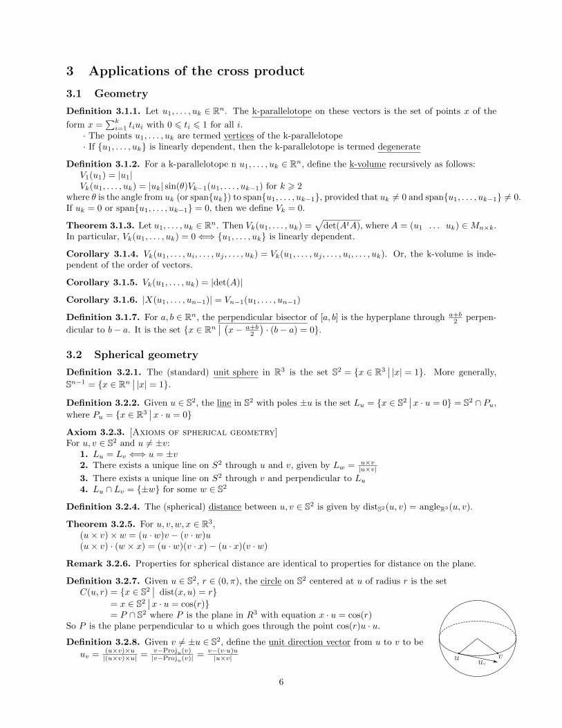
Definition 3.2.7. Given u ∈ S2, r ∈ (0, π), the circle on S2 centered at u of radius r is the setC(u, r) = {x ∈ S2

dist(x, u) = r}= x ∈ S2

x · u = cos(r)}= P ∩ S2 where P is the plane in R3 with equation x · u = cos(r)

So P is the plane perpendicular to u which goes through the point cos(r)u · u.

Definition 3.2.8. Given v 6= ±u ∈ S2, define the unit direction vector from u to v to be

uv = (u×v)×u|(u×v)×u| = v−Proju(v)

|v−Proju(v)|= v−(v·u)u

|u×v|

6

Remark 3.2.9. The set {u, uv} is an orthonormal basis for span{u, v}.

Remark 3.2.10. The line segment [u, v] ∈ S2 is given parametrically byx(t) = cos(t)u+ sin(t)uv with 0 6 t 6 dist(u, v) = cos−1(u · v)

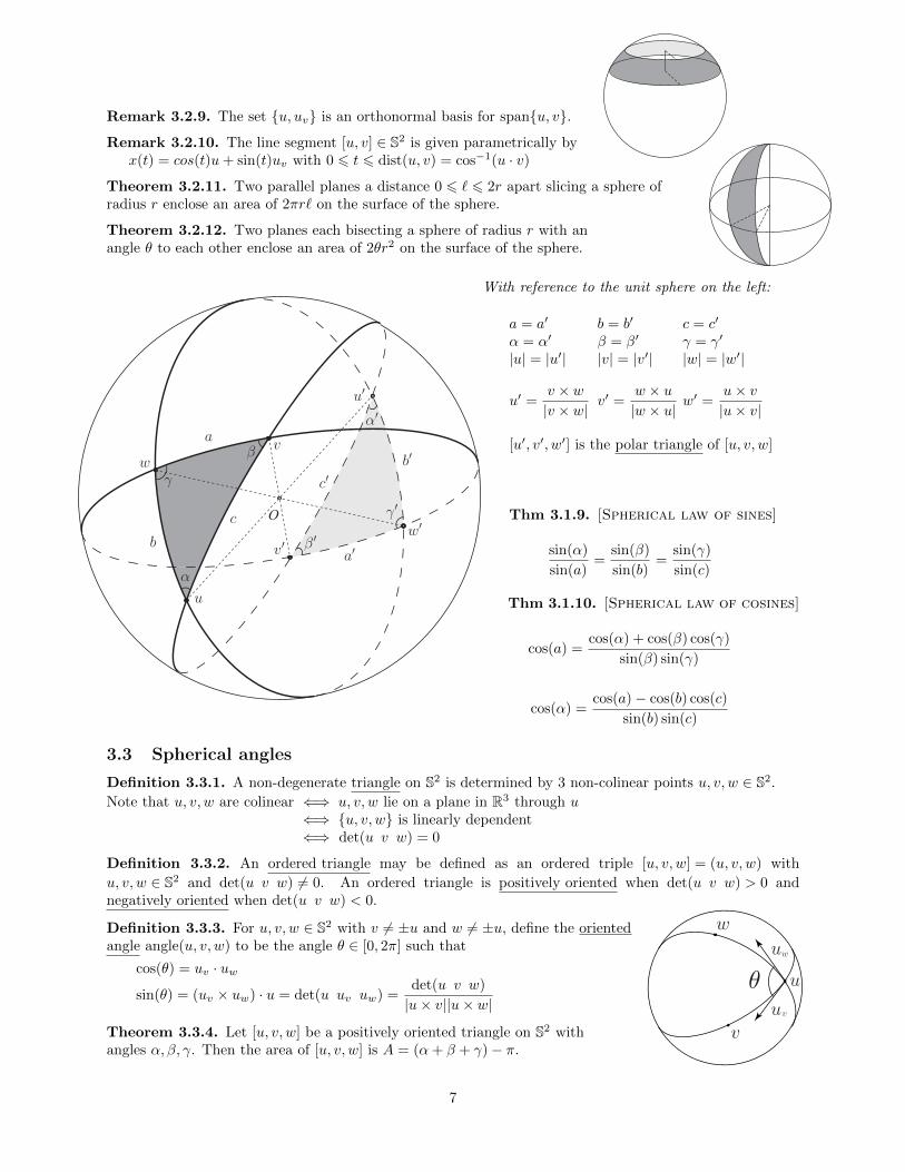
Theorem 3.2.11. Two parallel planes a distance 0 6 ` 6 2r apart slicing a sphere ofradius r enclose an area of 2πr` on the surface of the sphere.

Theorem 3.2.12. Two planes each bisecting a sphere of radius r with anangle θ to each other enclose an area of 2θr2 on the surface of the sphere.

O

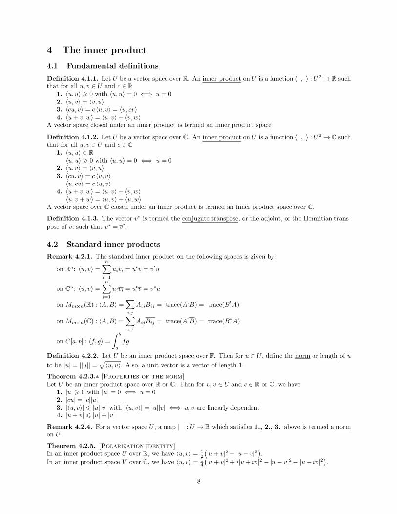
With reference to the unit sphere on the left:

a = a′ b = b′ c = c′

α = α′ β = β′ γ = γ′

|u| = |u′| |v| = |v′| |w| = |w′|

u′ =v × w|v × w|

v′ =w × u|w × u|

w′ =u× v|u× v|

[u′, v′, w′] is the polar triangle of [u, v, w]

Thm 3.1.9. [Spherical law of sines]

sin(α)

sin(a)=

sin(β)

sin(b)=

sin(γ)

sin(c)

Thm 3.1.10. [Spherical law of cosines]

cos(a) =cos(α) + cos(β) cos(γ)

sin(β) sin(γ)

cos(α) =cos(a)− cos(b) cos(c)

sin(b) sin(c)

3.3 Spherical angles

Definition 3.3.1. A non-degenerate triangle on S2 is determined by 3 non-colinear points u, v, w ∈ S2.

Note that u, v, w are colinear ⇐⇒ u, v, w lie on a plane in R3 through u⇐⇒ {u, v, w} is linearly dependent⇐⇒ det(u v w) = 0

Definition 3.3.2. An ordered triangle may be defined as an ordered triple [u, v, w] = (u, v, w) with

u, v, w ∈ S2 and det(u v w) 6= 0. An ordered triangle is positively oriented when det(u v w) > 0 andnegatively oriented when det(u v w) < 0.

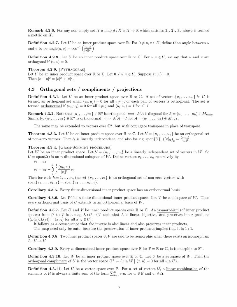
Definition 3.3.3. For u, v, w ∈ S2 with v 6= ±u and w 6= ±u, define the orientedangle angle(u, v, w) to be the angle θ ∈ [0, 2π] such that

cos(θ) = uv · uwsin(θ) = (uv × uw) · u = det(u uv uw) =

det(u v w)

|u× v||u× w|

Theorem 3.3.4. Let [u, v, w] be a positively oriented triangle on S2 withangles α, β, γ. Then the area of [u, v, w] is A = (α+ β + γ)− π.

7

4 The inner product

4.1 Fundamental definitions

Definition 4.1.1. Let U be a vector space over R. An inner product on U is a function 〈 , 〉 : U2 → R suchthat for all u, v ∈ U and c ∈ R

1. 〈u, u〉 > 0 with 〈u, u〉 = 0 ⇐⇒ u = 02. 〈u, v〉 = 〈v, u〉3. 〈cu, v〉 = c 〈u, v〉 = 〈u, cv〉4. 〈u+ v, w〉 = 〈u, v〉+ 〈v, w〉

A vector space closed under an inner product is termed an inner product space.

Definition 4.1.2. Let U be a vector space over C. An inner product on U is a function 〈 , 〉 : U2 → C suchthat for all u, v ∈ U and c ∈ C

1. 〈u, u〉 ∈ R〈u, u〉 > 0 with 〈u, u〉 = 0 ⇐⇒ u = 0

2. 〈u, v〉 = 〈v, u〉3. 〈cu, v〉 = c 〈u, v〉〈u, cv〉 = c 〈u, v〉

4. 〈u+ v, w〉 = 〈u, v〉+ 〈v, w〉〈u, v + w〉 = 〈u, v〉+ 〈u,w〉

A vector space over C closed under an inner product is termed an inner product space over C.

Definition 4.1.3. The vector v∗ is termed the conjugate transpose, or the adjoint, or the Hermitian trans-

pose of v, such that v∗ = vt.

4.2 Standard inner products

Remark 4.2.1. The standard inner product on the following spaces is given by:

on Rn: 〈u, v〉 =

n∑i=1

uivi = utv = vtu

on Cn: 〈u, v〉 =

n∑i=1

uivi = utv = v∗u

on Mm×n(R) : 〈A,B〉 =∑i,j

AijBij = trace(AtB) = trace(BtA)

on Mm×n(C) : 〈A,B〉 =∑i,j

AijBij = trace(AtB) = trace(B∗A)

on C[a, b] : 〈f, g〉 =

∫ b

a

fg

Definition 4.2.2. Let U be an inner product space over F. Then for u ∈ U , define the norm or length of u

to be |u| = ||u|| =√〈u, u〉. Also, a unit vector is a vector of length 1.

Theorem 4.2.3.∗ [Properties of the norm]Let U be an inner product space over R or C. Then for u, v ∈ U and c ∈ R or C, we have

1. |u| > 0 with |u| = 0 ⇐⇒ u = 02. |cu| = |c||u|3. |〈u, v〉| 6 |u||v| with |〈u, v〉| = |u||v| ⇐⇒ u, v are linearly dependent4. |u+ v| 6 |u|+ |v|

Remark 4.2.4. For a vector space U , a map | | : U → R which satisfies 1., 2., 3. above is termed a normon U .

Theorem 4.2.5. [Polarization identity]In an inner product space U over R, we have 〈u, v〉 = 1

2

(|u+ v|2 − |u− v|2

).

In an inner product space V over C, we have 〈u, v〉 = 14

(|u+ v|2 + i|u+ iv|2 − |u− v|2 − |u− iv|2

).

8

Remark 4.2.6. For any non-empty set X a map d : X ×X → R which satisfies 1., 2., 3. above is termeda metric on X.

Definition 4.2.7. Let U be an inner product space over R. For 0 6= u, v ∈ U , define than angle between u

and v to be angle(u, v) = cos−1(〈u,v〉|u||v|

)Definition 4.2.8. Let U be an inner product space over R or C. For u, v ∈ U , we say that u and v areorthogonal if 〈u, v〉 = 0.

Theorem 4.2.9. [Pythagoras]Let U be an inner product space over R or C. Let 0 6= u, v ∈ U . Suppose 〈u, v〉 = 0.Then |v − u|2 = |v|2 + |u|2.

4.3 Orthogonal sets / compliments / projections

Definition 4.3.1. Let U be an inner product space over R or C. A set of vectors {u1, . . . , un} in U istermed an orthogonal set when 〈ui, uj〉 = 0 for all i 6= j, or each pair of vectors is orthogonal. The set istermed orthonormal if 〈ui, uj〉 = 0 for all i 6= j and 〈ui, ui〉 = 1 for all i.

Remark 4.3.2. Note that {u1, . . . , uk} ∈ Rn is orthogonal ⇐⇒ AtA is diagonal forA = (u1 . . . uk) ∈Mn×k.Similarly, {u1, . . . , uk} ∈ Rn is orthonormal ⇐⇒ AtA = I for A = (u1 . . . uk) ∈Mn×k.

The same may be extended to vectors over Cn, but with conjugate transpose in place of transpose.

Theorem 4.3.3. Let U be an inner product space over R or C. Let U = {u1, . . . , un} be an orthogonal set

of non-zero vectors. Then U is linearly independent, and also for x ∈ span{U},([x]U

)k

= 〈x,uk〉|uk|2 .

Theorem 4.3.4. [Gram-Schmidt procedure]Let W be an inner product space. Let U = {u1, . . . , un} be a linearly independent set of vectors in W . SoU = span(U) is an n-dimensional subspace of W . Define vectors v1, . . . , vn recursively by

v1 = u1

vk = uk −k−1∑i=1

〈uk, vi〉|vi|2

vi

Then for each k = 1, . . . , n, the set {v1, . . . , vk} is an orthogonal set of non-zero vectors withspan{v1, . . . , vk−1} = span{u1, . . . , uk−1}.

Corollary 4.3.5. Every finite-dimensional inner product space has an orthonormal basis.

Corollary 4.3.6. Let W be a finite-dimensional inner product space. Let V be a subspace of W . Thenevery orthonormal basis of U extends to an orthonormal basis of W .

Definition 4.3.7. Let U and V be inner product spaces over R or C. An isomorphism (of inner productspaces) from U to V is a map L : U → V such that L is linear, bijective, and preserves inner products(〈L(x), L(y)〉 = 〈x, y〉 for all x, y ∈ U).

It follows as a consequence that the inverse is also linear and also preserves inner products.The map need only be onto, because the preservation of inner products implies that it is 1 : 1.

Definition 4.3.8. Two inner product spaces U, V are said to be isomorphic when there exists an isomorphismL : U → V .

Corollary 4.3.9. Every n-dimensional inner product space over F for F = R or C, is isomorphic to Fn.

Definition 4.3.10. Let W be an inner product space over R or C. Let U be a subspace of W . Then theorthogonal compliment of U is the vector space U⊥ = {x ∈W

〈x, u〉 = 0 for all u ∈ U}.

Definition 4.3.11. Let U be a vector space over F. For a set of vectors U , a linear combination of theelements of U is always a finite sum of the form

∑ni=1 ciui for ci ∈ F and ui ∈ U .

9

Theorem 4.3.12. [Properties of the orthogonal compliment]Let W be an inner product space over R or C, and let U be a subspace of W . Then

1. U ∩ U⊥ = {0}2. U ⊂ (U⊥)⊥

If W is finite-dimensional, then we also have3. If U = {u1, . . . , uk} is an orthogonal (orthonormal) basis for U , and W = {u1, . . . , uk, v1, . . . , v`} is an

orthogonal (orthonormal) basis for W , then V = V \ U = {v1, . . . , v`} is an orthogonal (orthonormal)basis for U⊥.

4. If U = {u1, . . . , uk} is an orthogonal (orthonormal) basis for U , and V = {v1, . . . , v`} is an orthogonal(orthonormal) basis for U⊥, then W = U ∪ V is an orthogonal (orthonormal) basis for W .

5. dim(U) + dim(U⊥) = dim(W )6. Given any x ∈W , there exist unique vectors u, v ∈W with u ∈ U and v ∈ U⊥ such that u+ v = w.7. W = U ⊕ U⊥

Theorem 4.3.13.∗[Orthogonal projections]Let W be a (possibly infinite-dimensional) inner product space over R or C and let U be a finite dimensionalsubspace of W . Then given x ∈W , there exist unique vectors u, v,∈W with u ∈ U and v ∈ U⊥ such thatu+ v = x. In addition, the vector u is the unique vector in U which is nearest to x.

Moreover, if U = {u1, . . . , un} is any orthogonal basis for U , then u =

n∑k=1

〈x, uk〉|uk|2

uk.

Definition 4.3.14. Let W be an inner product space over R or C and let U be a finite-dimensional subspace.Given x ∈W , the unique vector u in the above theorem is termed the orthogonal projection of x onto U ,and is expressed u = ProjU (x).

4.4 Quotient spaces

Definition 4.4.1. Let W be any vector space over F. Let U be a subspace of W . For any w ∈W , definethe coset of U containing w to be

{w}+ U = {w + uu ∈ U} = w + U

Definition 4.4.2. Let W be any vector space over F. Let U be a subspace of W . Then the quotient space,or the collection of all cosets of U , is the vector space

W/U = {p+ Up ∈W}

with (p+ U) + (q + U) = (p+ q) + Uc(p+ U) = cp+ U0 = 0 + U = U

Definition 4.4.3. The codimension of U in W is the dimension of W/U .

Definition 4.4.4. A hyperspace of W is a subspace of codimension 1.

Theorem 4.4.5. Let W be a vector space over F. Let U be a subspace of W . If U is a basis for U andU extends to a basis W for W , and if we let V =W \ U , then {v + U

v ∈ V} is a basis for W/U , and thedimension of the quotient space is the number of vectors in V, or the cardinality of V, and dim(W/U) = |V|.Further, if W is finite dimensional, then dim(U)+ dim(W/U) = dim(W ).

Theorem 4.4.6. With respect to the above, W ∼= U ⊕W/U , or W ∼= U ×W/U .

Definition 4.4.7. If U, V are subspaces of W with U ∩ V = {0} such that for all w ∈W , there existu ∈ U, v ∈ V with u+ v = w, then W is the internal direct sum of U and V , and we write W = U ⊕ V .

Definition 4.4.8. Given two vector spaces U, V , the external direct sum (or direct product) of U and V isthe vector space

10

U × V = {(u, v)u ∈ U, v ∈ V }

with (u1, v1) + (u2, v2) = (u1 + u2, v1 + v2)c(u+ v) = (cu+ cv)

Remark 4.4.9. If U, V are subspaces ofW , then U ⊕ V ∼= U × V . Also, U × {0} = {(u, 0)u ∈ U} ⊂ U × V .

Definition 4.4.10. Given a set A and vector spaces Uα with α ∈ A, define the direct sum of the spaces tobe the vector space∑

α∈AUα = {f : A→

⋃α∈A

Uαf(α) ∈ Uα for all α ∈ A with f(α) 6= 0 for only finitely many α ∈ A}

and we define the direct product of the vector spaces Uα to be∏α∈A

Uα = {f : A→⋃α∈A

Uαf(α) ∈ Uα for all α ∈ A}

When A is a finite, these are equal. When A is infinite,∑α∈A

Uα (∏α∈A

Uα

Theorem 4.4.11. Suppose L : W → V is linear. Then W/ker(L) ∼= Range(L) is an isomorphism given byL̄ : W/ker(L)→ Range(L) with L̄(p+ ker(L)) = L(p) ∈ L.

4.5 Dual spaces

Definition 4.5.1. Let U be a vector space over F. The dual vector space of U is the vector space

U∗ = Lin(U,F) = {f : U → Ff is linear}

Theorem 4.5.2.∗ Let U be a finite-dimensional vector space over F. Let U = {u1, . . . , un} be a basis forU . For k = 1, . . . , n, define fk ∈ U∗, so fk : U → F, to be the unique linear map with fk(ui) = δki. ThenF = {f1, . . . , fn} is a basis for U∗.

Definition 4.5.3. The set F = {f1, . . . , fn}in the above theorem is termed the dual basis of U for U .

Then f =

n∑k=1

f(uk)fk.

Definition 4.5.4. Let U, V be vector spaces over F. Let L : U → V be linear. Define the dual (or thetranspose) map Lt : V ∗ → U∗ given by Lt(g) = g ◦ L for all g ∈ V ∗.

Theorem 4.5.5. Let U, V be finite dimensional vector spaces over F. Let L : U → V be linear. U ,V be

bases for U, V . Let F ,G be the dual bases for U∗ and V ∗. Then [Lt]G

F=(

[L]U

V

)tDefinition 4.5.6. Let U be a vector space over F. The evaluation map E : U → U∗∗ is given byE(u)(f) = f(u) for all u ∈ U and f ∈ U∗.

Theorem 4.5.7. Let U be a finite dimensional vector space over F. Then the evaluation map E : U → U∗∗

is a (natural) isomorphism.

Remark 4.5.8. Given a basis U = {u1, . . . , un} for a vector space U , we obtain a (non-natural) isomorphismLU : U → U∗ given by LmF (ui) = fi. This is an isomorphism, since F = {f1, . . . , fn} is a basis for U∗.

Theorem 4.5.9. Let U be a finite dimensional inner product space over R or C. Given f ∈ U∗, there existsa unique vector u ∈ U such that f(x) = 〈x, u〉 for all x ∈ U .

Corollary 4.5.10. Let U be a finite dimensional inner product space over R. Then the map L : U → U∗

given by L(u)(x) = 〈x, u〉 is an isomorphism.

11

Definition 4.5.11. Let W be a vector space over F. Let U be a subspace of W . Then the annihilator of Uin W ∗ is the space V ◦ = {f ∈W ∗

f(u) = 0 for all u ∈ U}.

Theorem 4.5.12. Let U, V be finite-dimensional inner product spaces over R or C. Let L : U → V be alinear map. Then there exists a unique linear map L∗ : V → U such that 〈L(x), y〉 = 〈x, L∗(y)〉 for all x ∈ Uand y ∈ V .

Definition 4.5.13. The above map L∗ is termed the adjoint of L. In case U and/or V are infinite dimen-sional, such a map need not exist, but if it does, then it is termed the adjoint of L.

Corollary 4.5.14. Let U, V be finite dimensional inner product spaces. Let U ,V be orthonormal bases for

U, V . Let L : U → V be linear. Then [L∗]V

U=(

[L]U

V

)∗4.6 Normal linear maps, etc

Theorem 4.6.1. Let U, V be finite dimensional vector spaces over F. Let L : U → V be linear with

rank(L) = r. Then there exist bases U ,V for U and V such that [L]UV is of the form

(Ir 00 0

).

Lemma 4.6.2.∗ For every A ∈Mn×n(F) whose characteristic polynomial splits, there exists a unitary matrixP (and so P−1 = P ∗) such that T = P ∗AP is upper triangular. Further, the diagonal values of T are theeigenvalues of A, repeated by their algebraic multiplicity.

Theorem 4.6.3.∗ [Schur]Let U be a finite dimensional inner product space over R or C. Let L : U → U be linear. Suppose thecharacteristic polynomial fL splits over F (always occurs for C, for R only when eigenvalues (roots) are real).Then there exists an orthonormal basis U such that T = [L]U is upper triangular. Moreover, the diagonalvalues of T are the eigenvalues of L, repeated according to their algebraic multiplicity.

Remark 4.6.4. The following statements are equivalent:· The linear map L is diagonalizable.· There exists a basis of eigenvectors of L for L.· dim(Eλi

) = mi for all iwhere Eλi

is the eigenspace of the eigenvalue λi of L, and mi is the algebraic multiplicity of eigenvalue λi.

Definition 4.6.5. Let U be a finite-dimensional inner product space over F = R or C. Let L : U → V belinear. The map L is unitarily triangularziable if there exists an orthonormal basis U for U such that [L]Uis upper triangular. Similarly, L is unitarily diagonalizable if there exists an orthonormal basis U for U suchthat [L]U is diagonal.

Corollary 4.6.6. [from Schur, for F = C]Let U be a finite dimensional inner product space over C. Let L : U → U be linear.

1. L∗L = LL∗ ⇐⇒ L is unitarily diagonalizable2. L∗ = L ⇐⇒ L is unitarily diagonalizable and the eigenvalues of L are real.

L∗ = −L ⇐⇒ L is unitarily diagonalizable and the eigenvalues of L are imaginary.4. L∗L = I ⇐⇒ L is unitarily diagonalizable and the eigenvalues of L have unit norm.

Corollary 4.6.7. [from Schur, for F = R]Let U be a finite dimensional inner product space over R. Let L : U → U be linear.

1. L∗L = LL∗ ⇐⇒ L is orthogonally diagonalizable2. L∗ = L and L∗L = I ⇐⇒ L is orthogonally diagonalizable and every eigenvalue of L is ±1

Definition 4.6.8. Let U be an inner product space over R or C. Let L : U → U be linear.when L∗L = LL∗, then L is normalwhen L∗ = L, then L is self-adjoint or Hermitianwhen L∗ = L, then L is skew-Hermitianwhen L∗L = I, then L is unitary

12

Remark 4.6.9. For any field F, we have the following matrix groups:GL(n,F) = {A ∈Mn×n(F)

det(A) 6= 0} general linear groupSL(n,F) = {A ∈Mn×n(F)

det(A) = 1} special linear group - preserves orientationO(n,F) = {A ∈Mn×n(F)

AtA = I} orthogonal group - preserves distanceSO(n,F) = {A ∈Mn×n(F)

AtA = I, det(A) = 1} special orthogonal groupU(n,F) = {A ∈Mn×n(C)

A∗A = I} unitary groupSU(n,F) = {A ∈Mn×n(C)

A∗A = I, det(A) = 1} special unitary group

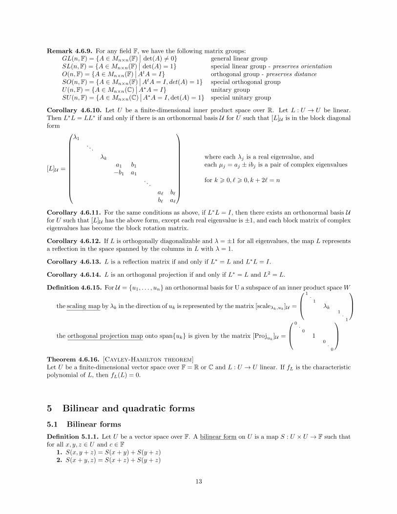
Corollary 4.6.10. Let U be a finite-dimensional inner product space over R. Let L : U → U be linear.Then L∗L = LL∗ if and only if there is an orthonormal basis U for U such that [L]U is in the block diagonalform

[L]U =

λ1. . .

λka1 b1−b1 a1

. . .

a` b`b` a`

where each λj is a real eigenvalue, andeach µj = aj ± ibj is a pair of complex eigenvalues

for k > 0, ` > 0, k + 2` = n

Corollary 4.6.11. For the same conditions as above, if L∗L = I, then there exists an orthonormal basis Ufor U such that [L]U has the above form, except each real eigenvalue is ±1, and each block matrix of complexeigenvalues has become the block rotation matrix.

Corollary 4.6.12. If L is orthogonally diagonalizable and λ = ±1 for all eigenvalues, the map L representsa reflection in the space spanned by the columns in L with λ = 1.

Corollary 4.6.13. L is a reflection matrix if and only if L∗ = L and L∗L = I.

Corollary 4.6.14. L is an orthogonal projection if and only if L∗ = L and L2 = L.

Definition 4.6.15. For U = {u1, . . . , un} an orthonormal basis for U a subspace of an inner product space W

the scaling map by λk in the direction of uk is represented by the matrix [scaleλk,uk]U =

1·1

λk1·1

the orthogonal projection map onto span{uk} is given by the matrix [Projuk

]U =

0·0

10·0

Theorem 4.6.16. [Cayley-Hamilton theorem]Let U be a finite-dimensional vector space over F = R or C and L : U → U linear. If fL is the characteristicpolynomial of L, then fL(L) = 0.

5 Bilinear and quadratic forms

5.1 Bilinear forms

Definition 5.1.1. Let U be a vector space over F. A bilinear form on U is a map S : U × U → F such thatfor all x, y, z ∈ U and c ∈ F

1. S(x, y + z) = S(x+ y) + S(y + z)2. S(x+ y, z) = S(x+ z) + S(y + z)

13

3. S(cx, y) = c · S(x, y) = S(x, cy)A bilinear form S is symmetric if S(x, y) = S(y, x)A bilinear form is skew-symmetric or alternating if S(x, y) = −S(y, x)A bilinear form is non-degenerate if S(u, x) = 0 for all x ∈ U ⇐⇒ u = 0 for all u ∈ U

Remark 5.1.2. If U is a basis for U , then a bilinear form S on U is determined completely by the valuesS(u, v) for u, v ∈ U . Indeed, if we have x =

∑ni=1 tiui and y =

∑nj=1 rjuj for ui, uj ∈ U , then

S(x, y) = S(∑n

i=1 tiui,∑nj=1 riui

)=∑i,j tirjS(ui, uj)

Note that this argument also holds for the infinite-dimensional case, since linear combinations are still finite.

Remark 5.1.3. Bilin(U × U) ∼=∏

(u,v)∈U×U

F

Definition 5.1.4. Let U be a finite dimensional vector space over F. Let S : U × U → F be a bilinear form.Let U be a basis for U . Then the matrix of S with respect to the basis U is defined to be the matrix [S]U

such that S(u, v) = [u]tU [S]U [v]U . Furthermore, the (i, j) entry of [S]U is S(ui, uj).

Remark 5.1.5. Let U be a finite-dimensional vector space over F. Let S : U × U be a bilinear form. Let

U ,V be bases for U . Then [S]V = [I]VUt[S]U [I]VU .

Definition 5.1.6. For A,B ∈Mn×n(F), we say that A and B are congruent if there exists an invertiblematrix Q such that B = QtAQ. Note that congruent matrices have the same rank.

Definition 5.1.7. The rank of a bilinear form S on a finite dimensional vector space U is the rank of [S]U

for any basis U of U .

Remark 5.1.8. A bilinear form S on a finite-dimensional vector space U is symmetric ⇐⇒ the matrix[S]U is symmetric for any basis U of U .

Theorem 5.1.9. Let U be a finite-dimensional vector space over F. Let S be a symmetric bilinear form.1. If char(F) 6= 2, (that is, 1 + 1 6= 0), then there exists a basis U for U such that [S]U is diagonal.2. If F = C, then there exists a basis U such that [S]U =

(Ir 00 0

)for r = rank(S).

3. If F = R, then there exists a basis U for U such that [S]U =

(Ik−Ir−k

0

)for some k.

4. If F = R, then there exists an orthonormal basis U for U such that [S]U =

λ1

. . .λk

0

for non-zero

eigenvalues λ1, . . . , λk of [S]U .5. If F = R and D = [S]U is diagonal for U a basis for U , then the number of positive entries of D does

not depend on U .

Theorem 5.1.10. [Sylvester]Let U be a finite-dimensional vector space over U . Let S : U × U → R be a symmetric bilinear form. Let Uand V be two bases for U such that [S]U and [S]V are both diagonal. Then the number of positive entries in[S]U is the number of positive entries in [S]V .

Remark 5.1.11. We write Bilin(U) = Bilin(U × U,F) for the space of bilinear forms S : U × U → F. Givena basis U of n-dimensional U , the map ψn : Bilin(U)→Mn×n(F) is a vector space isomorphic map.

Remark 5.1.12. An inner product in a real inner product space is a positive definite symmetric bilinearform. Also, a bilinear form S : U × U → R is non-degenerate when S(u, x) = 0 for all x ∈ U ⇐⇒ u = 0 forall u ∈ U .

14

5.2 Quadratic forms

Definition 5.2.1. A polynomial f ∈ F[x1, x2, . . . , xn] is of the form

f(x1, x2, . . . , xn) =∑

06i1,...,in

ai1,...,inxi11 · · ·xinn

with only finitely many of the ai1,...,in = 0.

Definition 5.2.2. A polynomial homogeneous of degree d may be expressed as

K(x) =

m∑d=0

∑06i1,...,in

i1+···+in=d

ai1,...,inxi11 · · ·xinn

Definition 5.2.3. Let U be a vector space over F. A quadratic form on U is a map K : U → F of the formK(u) = S(u, u) for some symmetric bilinear form S. If char(F) 6= 2, then

K(u+ v) = S(u+ v, u+ v) = S(u, u) + 2S(u, v) + S(v, v) = K(u) + 2S(u, v) +K(v)

Theorem 5.2.4. A quadratic form may be diagonalized if char(F) 6= 2.

Theorem 5.2.5. Let U be an n-dimensional vector space over R. Let K : U → R be a quadratic form onU , and let S : U × U → R be the corresponding symmetric bilinear form. Then the following are equivalent:

1. K (or S) is positive definite2. the eigenvalues of [K]U = [S]U are all positive for some (hence any) basis U for U3. for A = [K]U = [S]U we have det(Ak×k) > 0 with 1 6 k 6 n

Remark 5.2.6. For A ∈Mn×m(F) the notation Ak×` denotes the k × ` upper left submatrix of A such that1 6 k 6 n and 1 6 ` 6 m.

5.3 Characterization and extreme values

Recall that K : U → R or S : U × U → R is positive definite or symmetric bilinear when K(u) = S(u, u) > 0for u 6= 0.

Theorem 5.3.1.∗[Characterization of positive definite forms]Let U be an n-dimensional inner product space over R. Let K : U → R be a quadratic form on U , and letS : U × U → R be the corresponding symmetric bilinear form. Then the following statements are equivalent:

1. K (or S) is positive definite2. the eigenvalues of [K]U = [S]U are all positive for some (hence any) basis U for U3. for A = [K]U = [S]U we have det(Ak×k) > 0

where Ak×k represents the k × k upper-left submatrix of A.

Theorem 5.3.2. Let A ∈Mn×n(F). Suppose A∗ = A. Recall that the eigenvalues of A are real. Letλ1,6 λ2 6 · · · 6 λn be the eigenvalues of A listed according to algebraic multiplicity in increasing order.Then max

|x|=1{x∗Ax} = λn and min

|x|=1{x∗Ax} = λ1.

Corollary 5.3.3. Let U be an n-dimensional inner product space over R. Let S : U × U → R be a symmetricbilinear form and let K : U → R be the corresponding quadratic form on U . Let λ1,6 λ2 6 · · · 6 λn be theeigenvalues listed according to algebraic multiplicity in increasing order, of [K]U = [S]U for some (hence any)orthonormal basis U for U . Then max

|u|=1{K(u)} = λn and min

|u|=1{K(u)} = λ1.

Definition 5.3.4. Let U, V be inner product spaces over F. If a map L : U → V has an adjoint, then definethe singular values of L to be the square roots of the eigenvalues of L∗L.

Let U, V be finite dimensional inner product spaces over F. Let L : U → V be linear. Let0 6 σ1 6 σ2 6 · · · 6 σn be the singular values of L listed in increasing order, repeated according to alge-braic multiplicity. Then max

|u|=1{|L(u)|} = σn and min

|u|=1{|L(u)|} = σ1.

15

Definition 5.3.5. The spectrum of a linear map L : U → U over an inner product space U is the set ofeigenvalues of L.

Theorem 5.3.6.∗ Let U, V be inner product spaces over F. Let L : U → V be linear. Then there existorthonormal bases U ,V for U, V such that [L]UV is in the form

[L]UV = Σ =

σ1

. . . 0σr

0 0

Corollary 5.3.7. For A ∈Mm×n(F), there exist P ∈Mm×n(F) and Q ∈Mn×n(F) with P ∗P = Im andQ∗Q = In such that

P ∗AQ = Σ =

σ1

. . . 0σr

0 0

This is termed the singular value decomposition of A = [L]U with the singular values as described above.

6 Jordan normal form

6.1 Block form

Definition 6.1.1. The m×m Jordan block for the eigenvalue λ ∈ F over F is the m×m matrix

Jmλ =

λ 1

. . .. . .

. . . 1λ

Definition 6.1.2. A matrix B ∈Mn×n(F) is in Jordan form when it is in the block diagonal form

B =

Jm1

λ1

Jm2

λ2

. . .

Jm`

λ`

6.2 Canonical form

Theorem 6.2.1. Let U be a finite-dimensional vector space over F. Let L : U → U be linear. Suppose thatthe characteristic polynomial fL(t) of L splits over F. Then there exists a basis U for U such that [L]U = Bis in Jordan form. The matrix B is uniquely determined by L up to the order of the Jordan blocks.

Definition 6.2.2. A generalized eigenvector of a map L : U → U for an eigenvalue λ of L is a non-zero

vector u ∈ U such that (L− λI)Pu = 0 for some p > 0.

Definition 6.2.3. A cycle of generalized eigenvectors of length m for the eigenvalue λ is an ordered set ofvectors C = {u1, . . . , um} such that

um−1 = (L− λI)um

um−2 = (L− λI)2um

...

u1 = (L− λI)m−1um

0 = (L− λI)mum

16

Definition 6.2.4. The generalized eigenspace for λ is Kλ = {u ∈ U(L− λI)pu = 0 for some p > 0}

Theorem 6.2.5.∗ Let U be a finite-dimensional vector space over F with L : U → U linear. Then for everyeigenvalue λ of L, there exists a basis of cycles corresponding to λ for Kλ.

Definition 6.2.6. Let L : U → U for U a finite-dimensional vector space over F be linear. Theminimal polynomial of L is the unique monic polynomial fL(x) of minimum possible degree such thatfL(L) = 0.

Note that the minimal polynomial is always a factor of the characteristic polynomial, and the roots of theminimal polynomial are the same as the roots of the characteristic polynomial.

17

7 Selected proofs

Theorem 4.2.3. [Properties of the norm]Let U be an inner product space over R or C. Then for u, v ∈ U and c ∈ R or C, we have

1. |u| > 0 with |u| = 0 ⇐⇒ u = 02. |cu| = |c||u|3. |〈u, v〉| 6 |u||v| with |〈u, v〉| = |u||v| ⇐⇒ u, v are linearly dependent4. |u+ v| 6 |u|+ |v|

Proof: For 2.:

|cu|2 = 〈cu, cu〉 = c 〈u, cu〉 = cc 〈u, u〉 = |c|2 |u|2 =⇒ |cu| = |c||u|

For 3.: Suppose {u, v} is linearly dependent, say u = cv for c ∈ C.

|〈u, v〉| = |c 〈v, v〉| = |c||v|2 = |cv||v| = |u||v|

Suppose {u, v} is linearly independent.

〈v − Projuv, u〉 =

⟨v − 〈v, u〉〈u, u〉

u, u

⟩= 〈v, u〉 −

⟨〈v, u〉〈u, u〉

u, u

⟩= 〈v, u〉 − 〈v, u〉

〈u, u〉〈u, u〉 = 0

Since {u, v} is linearly independent, v − 〈v,u〉〈u,u〉u 6= 0, so

0 <

v − 〈v, u〉〈u, u〉u

2

=

⟨v − 〈v, u〉〈u, u〉

u, v − 〈v, u〉〈u, u〉

u

⟩=

⟨v − 〈v, u〉〈u, u〉

u, v

⟩− 0 = 〈v, v〉 − 〈v, u〉

〈u, u〉〈u, v〉

〈v, u〉 〈u, v〉 < 〈u, u〉 〈v, v〉

〈v, u〉 〈v, u〉 < |u|2 |v|2

|〈u, v〉|2 < |u|2 |v|2

|〈u, v〉| < |u| |v|

For 4.:

|u+ v|2 = 〈u+ v, u+ v〉= 〈u, u〉+ 〈u, v〉+ 〈v, u〉+ 〈v, v〉

= |u|2 + 〈u, v〉+ 〈u, v〉+ |v|2

= |u|2 + 2Re(〈u, v〉) + |v|2

6 |u|2 + 2 |Re(〈u, v〉)|+ |v|2

6 |u|2 + 2 |〈u, v〉|+ |v|2

6 |u|2 + 2 |u||v|+ |v|2

= (|u|+ |v|)2

|u+ v| 6 |u|+ |v|

18

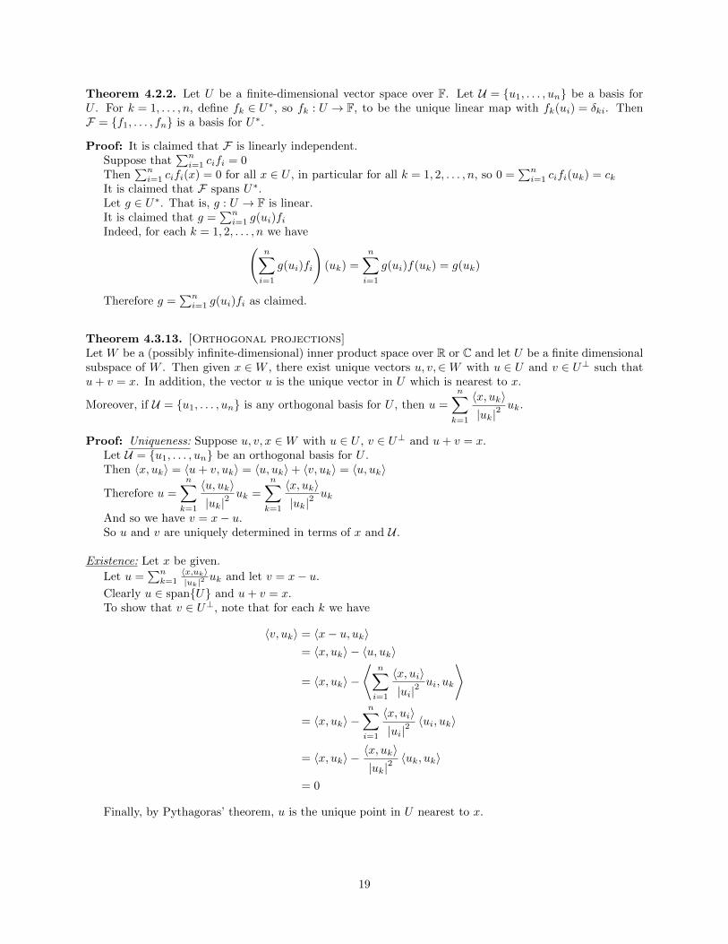
Theorem 4.2.2. Let U be a finite-dimensional vector space over F. Let U = {u1, . . . , un} be a basis forU . For k = 1, . . . , n, define fk ∈ U∗, so fk : U → F, to be the unique linear map with fk(ui) = δki. ThenF = {f1, . . . , fn} is a basis for U∗.

Proof: It is claimed that F is linearly independent.Suppose that

∑ni=1 cifi = 0

Then∑ni=1 cifi(x) = 0 for all x ∈ U , in particular for all k = 1, 2, . . . , n, so 0 =

∑ni=1 cifi(uk) = ck

It is claimed that F spans U∗.Let g ∈ U∗. That is, g : U → F is linear.It is claimed that g =

∑ni=1 g(ui)fi

Indeed, for each k = 1, 2, . . . , n we have(n∑i=1

g(ui)fi

)(uk) =

n∑i=1

g(ui)f(uk) = g(uk)

Therefore g =∑ni=1 g(ui)fi as claimed.

Theorem 4.3.13. [Orthogonal projections]Let W be a (possibly infinite-dimensional) inner product space over R or C and let U be a finite dimensionalsubspace of W . Then given x ∈W , there exist unique vectors u, v,∈W with u ∈ U and v ∈ U⊥ such thatu+ v = x. In addition, the vector u is the unique vector in U which is nearest to x.

Moreover, if U = {u1, . . . , un} is any orthogonal basis for U , then u =

n∑k=1

〈x, uk〉|uk|2

uk.

Proof: Uniqueness: Suppose u, v, x ∈W with u ∈ U , v ∈ U⊥ and u+ v = x.Let U = {u1, . . . , un} be an orthogonal basis for U .Then 〈x, uk〉 = 〈u+ v, uk〉 = 〈u, uk〉+ 〈v, uk〉 = 〈u, uk〉

Therefore u =

n∑k=1

〈u, uk〉|uk|2

uk =

n∑k=1

〈x, uk〉|uk|2

uk

And so we have v = x− u.So u and v are uniquely determined in terms of x and U .

Existence: Let x be given.

Let u =∑nk=1

〈x,uk〉|uk|2

uk and let v = x− u.

Clearly u ∈ span{U} and u+ v = x.To show that v ∈ U⊥, note that for each k we have

〈v, uk〉 = 〈x− u, uk〉= 〈x, uk〉 − 〈u, uk〉

= 〈x, uk〉 −

⟨n∑i=1

〈x, ui〉|ui|2

ui, uk

⟩

= 〈x, uk〉 −n∑i=1

〈x, ui〉|ui|2

〈ui, uk〉

= 〈x, uk〉 −〈x, uk〉|uk|2

〈uk, uk〉

= 0

Finally, by Pythagoras’ theorem, u is the unique point in U nearest to x.

19

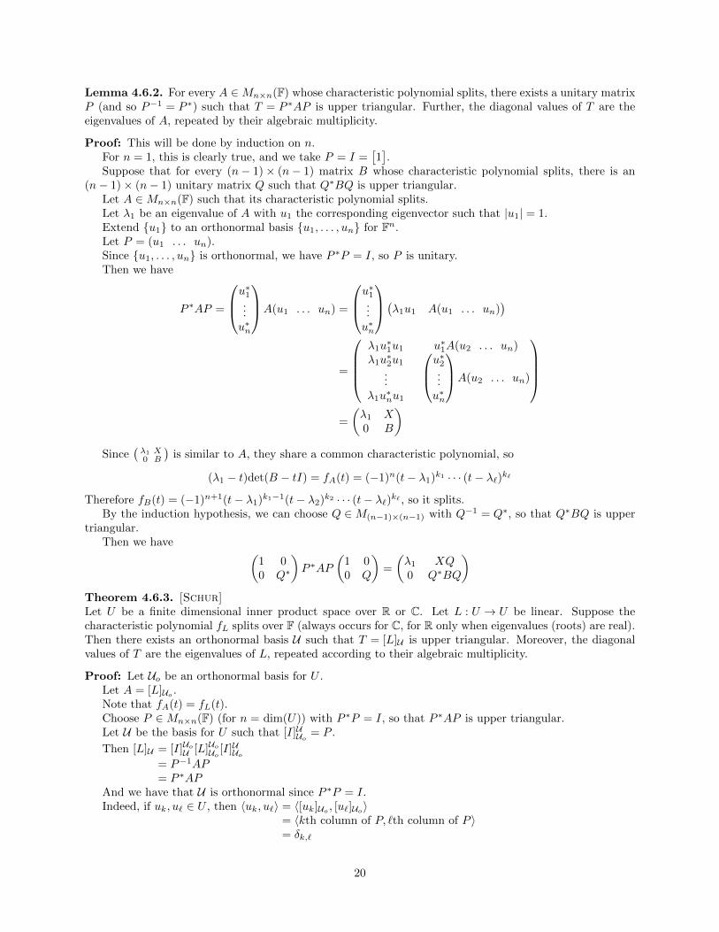
Lemma 4.6.2. For every A ∈Mn×n(F) whose characteristic polynomial splits, there exists a unitary matrixP (and so P−1 = P ∗) such that T = P ∗AP is upper triangular. Further, the diagonal values of T are theeigenvalues of A, repeated by their algebraic multiplicity.

Proof: This will be done by induction on n.For n = 1, this is clearly true, and we take P = I =

[1].

Suppose that for every (n− 1)× (n− 1) matrix B whose characteristic polynomial splits, there is an(n− 1)× (n− 1) unitary matrix Q such that Q∗BQ is upper triangular.

Let A ∈Mn×n(F) such that its characteristic polynomial splits.Let λ1 be an eigenvalue of A with u1 the corresponding eigenvector such that |u1| = 1.Extend {u1} to an orthonormal basis {u1, . . . , un} for Fn.Let P = (u1 . . . un).Since {u1, . . . , un} is orthonormal, we have P ∗P = I, so P is unitary.Then we have

P ∗AP =

u∗1...u∗n

A(u1 . . . un) =

u∗1...u∗n

(λ1u1 A(u1 . . . un))

=

λ1u

∗1u1 u∗1A(u2 . . . un)

λ1u∗2u1...

λ1u∗nu1

u∗2...u∗n

A(u2 . . . un)

=

(λ1 X0 B

)Since

(λ1 X0 B

)is similar to A, they share a common characteristic polynomial, so

(λ1 − t)det(B − tI) = fA(t) = (−1)n(t− λ1)k1 · · · (t− λ`)k`

Therefore fB(t) = (−1)n+1(t− λ1)k1−1(t− λ2)k2 · · · (t− λ`)k` , so it splits.By the induction hypothesis, we can choose Q ∈M(n−1)×(n−1) with Q−1 = Q∗, so that Q∗BQ is upper

triangular.Then we have (

1 00 Q∗

)P ∗AP

(1 00 Q

)=

(λ1 XQ0 Q∗BQ

)Theorem 4.6.3. [Schur]Let U be a finite dimensional inner product space over R or C. Let L : U → U be linear. Suppose thecharacteristic polynomial fL splits over F (always occurs for C, for R only when eigenvalues (roots) are real).Then there exists an orthonormal basis U such that T = [L]U is upper triangular. Moreover, the diagonalvalues of T are the eigenvalues of L, repeated according to their algebraic multiplicity.

Proof: Let Uo be an orthonormal basis for U .Let A = [L]Uo .Note that fA(t) = fL(t).Choose P ∈Mn×n(F) (for n = dim(U)) with P ∗P = I, so that P ∗AP is upper triangular.Let U be the basis for U such that [I]UUo = P .

Then [L]U = [I]UoU [L]UoUo [I]UUo= P−1AP= P ∗AP

And we have that U is orthonormal since P ∗P = I.Indeed, if uk, u` ∈ U , then 〈uk, u`〉 = 〈[uk]Uo , [u`]Uo〉

= 〈kth column of P, `th column of P 〉= δk,`

20

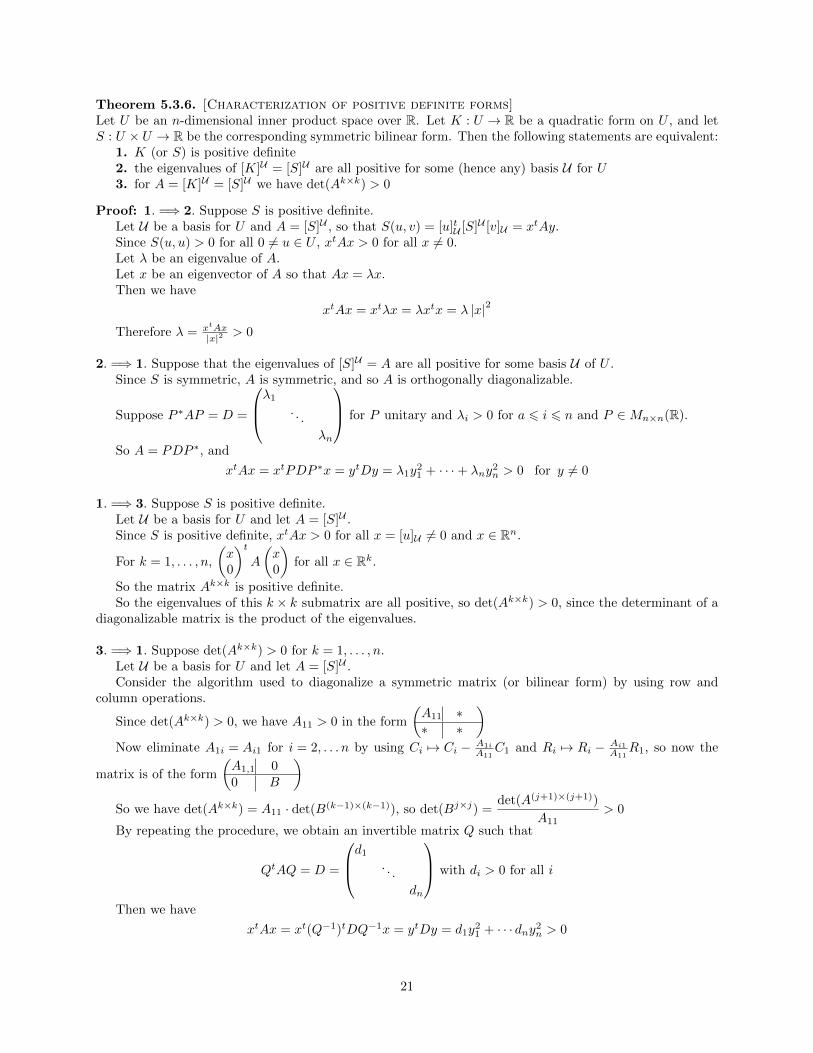
Theorem 5.3.6. [Characterization of positive definite forms]Let U be an n-dimensional inner product space over R. Let K : U → R be a quadratic form on U , and letS : U × U → R be the corresponding symmetric bilinear form. Then the following statements are equivalent:

1. K (or S) is positive definite2. the eigenvalues of [K]U = [S]U are all positive for some (hence any) basis U for U3. for A = [K]U = [S]U we have det(Ak×k) > 0

Proof: 1. =⇒ 2. Suppose S is positive definite.Let U be a basis for U and A = [S]U , so that S(u, v) = [u]tU [S]U [v]U = xtAy.Since S(u, u) > 0 for all 0 6= u ∈ U , xtAx > 0 for all x 6= 0.Let λ be an eigenvalue of A.Let x be an eigenvector of A so that Ax = λx.Then we have

xtAx = xtλx = λxtx = λ |x|2

Therefore λ = xtAx|x|2 > 0

2. =⇒ 1. Suppose that the eigenvalues of [S]U = A are all positive for some basis U of U .Since S is symmetric, A is symmetric, and so A is orthogonally diagonalizable.

Suppose P ∗AP = D =

λ1 . . .

λn

for P unitary and λi > 0 for a 6 i 6 n and P ∈Mn×n(R).

So A = PDP ∗, and

xtAx = xtPDP ∗x = ytDy = λ1y21 + · · ·+ λny

2n > 0 for y 6= 0

1. =⇒ 3. Suppose S is positive definite.Let U be a basis for U and let A = [S]U .Since S is positive definite, xtAx > 0 for all x = [u]U 6= 0 and x ∈ Rn.

For k = 1, . . . , n,

(x0

)tA

(x0

)for all x ∈ Rk.

So the matrix Ak×k is positive definite.So the eigenvalues of this k × k submatrix are all positive, so det(Ak×k) > 0, since the determinant of a

diagonalizable matrix is the product of the eigenvalues.

3. =⇒ 1. Suppose det(Ak×k) > 0 for k = 1, . . . , n.Let U be a basis for U and let A = [S]U .Consider the algorithm used to diagonalize a symmetric matrix (or bilinear form) by using row and

column operations.

Since det(Ak×k) > 0, we have A11 > 0 in the form

(A11 ∗∗ ∗

)Now eliminate A1i = Ai1 for i = 2, . . . n by using Ci 7→ Ci − A1i

A11C1 and Ri 7→ Ri − Ai1

A11R1, so now the

matrix is of the form

(A1,1 00 B

)So we have det(Ak×k) = A11 · det(B(k−1)×(k−1)), so det(Bj×j) =

det(A(j+1)×(j+1))

A11> 0

By repeating the procedure, we obtain an invertible matrix Q such that

QtAQ = D =

d1 . . .

dn

with di > 0 for all i

Then we have

xtAx = xt(Q−1)tDQ−1x = ytDy = d1y21 + · · · dny2n > 0

21

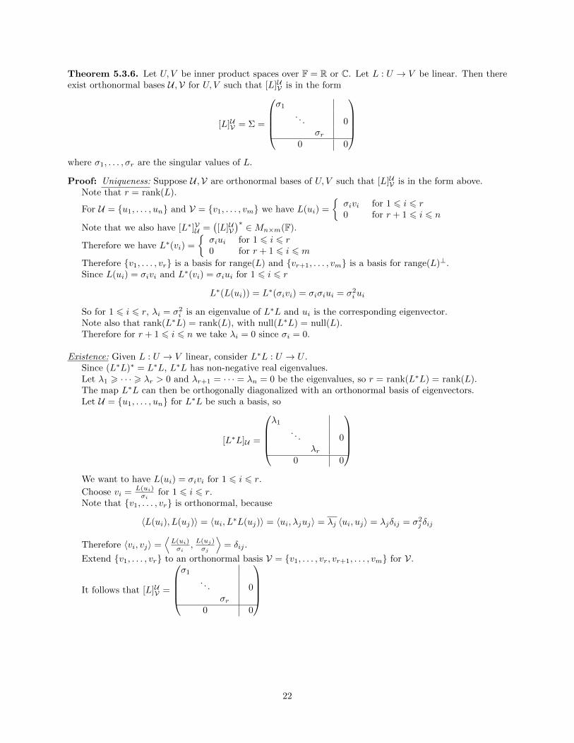
Theorem 5.3.6. Let U, V be inner product spaces over F = R or C. Let L : U → V be linear. Then thereexist orthonormal bases U ,V for U, V such that [L]UV is in the form

[L]UV = Σ =

σ1

. . . 0σr

0 0

where σ1, . . . , σr are the singular values of L.

Proof: Uniqueness: Suppose U ,V are orthonormal bases of U, V such that [L]UV is in the form above.Note that r = rank(L).

For U = {u1, . . . , un} and V = {v1, . . . , vm} we have L(ui) =

{σivi for 1 6 i 6 r0 for r + 1 6 i 6 n

Note that we also have [L∗]VU =([L]UV

)∗ ∈Mn×m(F).

Therefore we have L∗(vi) =

{σiui for 1 6 i 6 r0 for r + 1 6 i 6 m

Therefore {v1, . . . , vr} is a basis for range(L) and {vr+1, . . . , vm} is a basis for range(L)⊥.Since L(ui) = σivi and L∗(vi) = σiui for 1 6 i 6 r

L∗(L(ui)) = L∗(σivi) = σiσiui = σ2i ui

So for 1 6 i 6 r, λi = σ2i is an eigenvalue of L∗L and ui is the corresponding eigenvector.

Note also that rank(L∗L) = rank(L), with null(L∗L) = null(L).Therefore for r + 1 6 i 6 n we take λi = 0 since σi = 0.

Existence: Given L : U → V linear, consider L∗L : U → U .Since (L∗L)∗ = L∗L, L∗L has non-negative real eigenvalues.Let λ1 > · · · > λr > 0 and λr+1 = · · · = λn = 0 be the eigenvalues, so r = rank(L∗L) = rank(L).The map L∗L can then be orthogonally diagonalized with an orthonormal basis of eigenvectors.Let U = {u1, . . . , un} for L∗L be such a basis, so

[L∗L]U =

λ1

. . . 0λr

0 0

We want to have L(ui) = σivi for 1 6 i 6 r.

Choose vi = L(ui)σi

for 1 6 i 6 r.Note that {v1, . . . , vr} is orthonormal, because

〈L(ui), L(uj)〉 = 〈ui, L∗L(uj)〉 = 〈ui, λjuj〉 = λj 〈ui, uj〉 = λjδij = σ2j δij

Therefore 〈vi, vj〉 =⟨L(ui)σi

,L(uj)σj

⟩= δij .

Extend {v1, . . . , vr} to an orthonormal basis V = {v1, . . . , vr, vr+1, . . . , vm} for V.

It follows that [L]UV =

σ1

. . . 0σr

0 0

22

Theorem 6.2.5. Let U be a finite-dimensional vector space over F with L : U → U linear. Then for everyeigenvalue λ of L, there exists a basis of cycles corresponding to λ for Kλ.

Proof: Fix an eigenvalue λ of L.Choosem so that U = range(L− λI)0 ) range(L− λI)1 ) · · · ) range(L− λI)m = range(L− λI)m+1 = · · ·Previously we saw that range(L− λI)m =

⊕µ6=λ

Kµ for an eigenvalue µ of L.

We also have that {0} = null(L− λI)0 ( null(L− λI)1 ( · · · ( null(L− λI)m = null(L− λI)m+1 = · · ·Note that null(L− λI) = Eλ and null(L− λI)m = Kλ.Now follows the algorithm for finding a basis of cycles for Kλ.Step 1. Choose a basis {u11, . . . , u

`11 } for range(L− λI)m−1 ∩Kλ = range(L− λI)m−1 ∩ Eλ.

Then we obtain cycles {u11}, {u21}, . . . , {u`11 }.

Step 2. For 1 6 j 6 `1, choose uj2 ∈ range(L− λI)m−2 ∩Kλ so that (L− λI)uj2 = uj1.Also, extend {u11, . . . , u

`11 } to a basis {u11, . . . , u

`21 } for range(L− λI)m−2 ∩ Eλ .

We obtain the cycles {u11, u12}, . . . , {u`11 , u

`12 }, {u

`1+11 }, . . . , {u`21 }

Step k: Suppose we have constructed cycles Bj = {uj1, . . . , ujnj−1} for 1 6 j 6 `k−1 such that

{u11, . . . , u`k−1

1 } is a basis for range(L− λI)m−(k−1) ∩ Eλ and such that

`k−1⋃j=1

Bj is a basis for range(L− λI)m−(k−1) ∩Kλ.

For 1 6 j 6 `k−1, choose ujnj∈ range(L− λI)m−k ∩Kλ so that (L− λI)ujnj

= ujnj−1.

Then let Cj = {uj1, . . . , ujnj} = Bj ∪ {ujnj

} .

Also, extend {u11, . . . , u`k−1

1 } to a basis {u11, . . . , u`k1 } for range(L− λI)m−k ∩ Eλ.

Now it is claimed that

`k⋃j=1

Cj is a basis for range(L− λI)m−k ∩Kλ.

To see that⋃Cj is linearly independent, let

V = span⋃Cj ⊂ range(L− λI)m−k ∩Kλ

W = span⋃Bj = range(L− λI)m−(k−1) ∩Kλ

M = the restriction M = (L− λI) : V →W

Note that null(M) = range(L− λI)m−k ∩ Eλ and nullity(M) = `k by definition, so M is onto.Therefore

dim(V ) = rank(M) + nullity(M) = dim(W ) + `k =⋃Bj+ `k =

⋃CjTherefore

⋃Cj is a basis for V .

Therefore⋃Cj is linearly independent.

To see that⋃Cj spans range(L− λI)m−k ∩Kλ, let

V2 = range(L− λI)m−k ∩Kλ

W = range(L− λI)m−(k−1) ∩Kλ

M2 = the restrictionM2 = (L− λI) : V2 →W

Now we have that M2 is onto and null(M2) = range(L− λI)m−k ∩ Eλ with nullity(M2) = `k.So then

dim(V2) = dim(W ) + `k =⋃Bj+ `k =

⋃Cj = dim(V )

Therefore V2 = V = span⋃Cj .

23