MATH 212 NE 217 Douglas Wilhelm Harder Department of Electrical and Computer Engineering University of Waterloo Waterloo, Ontario, Canada Copyright © 2011 by Douglas Wilhelm Harder. All rights reserved. Advanced Calculus 2 for Electrical Engineering Advanced Calculus 2 for Nanotechnology Engineering Finite-Element Methods in Two Dimensions

MATH 212 NE 217 Douglas Wilhelm Harder Department of Electrical and Computer Engineering University of Waterloo Waterloo, Ontario, Canada Copyright © 2011.
Dec 24, 2015
Welcome message from author
This document is posted to help you gain knowledge. Please leave a comment to let me know what you think about it! Share it to your friends and learn new things together.
Transcript

MATH 212NE 217
Douglas Wilhelm Harder
Department of Electrical and Computer Engineering
University of Waterloo
Waterloo, Ontario, Canada
Copyright © 2011 by Douglas Wilhelm Harder. All rights reserved.
Advanced Calculus 2 for Electrical EngineeringAdvanced Calculus 2 for Nanotechnology Engineering
Finite-Element Methodsin Two Dimensions

Finite-element Methods in Two Dimensions
2
Outline
This topic discusses an introduction to finite-element methods in two dimensions– What we did in one dimension
– Dividing up a 2-D region
– Defining planar test functions on those regions
– Converting the test functions to systems of linear equations
– Solving the system
– Examples
Finite-element Methods in Two Dimensions
3
Outcomes Based Learning Objectives
By the end of this laboratory, you will:– You will understand dividing regions into triangular sub-regions
(tessellations)
– Understand the mathematical theory for performing finite-element methods in two dimensions

Finite-element Methods in Two Dimensions
4
Integration-by-Parts in Higher Dimensions
Before we start, we need a higher-dimensional version of integration by parts:– Using the properties of the gradient:
– Now use a corollary of Stokes’ theorem:
R R R
uv u v v u
u v uv v u
u v dxdy uv dxdy v u dxdy
R R R
u v dxdy uvd v u dxdy
s
Ref: http://en.wikipedia.org/wiki/Vector_calculus_identities

Finite-element Methods in Two Dimensions
5
Integration-by-Parts in Higher Dimensions
This variation has the product of two scalar-valued functions replaced with a product of scalar- and vector-valued functions – Using the properties of the gradient:
– Now use a corollary of Stokes’ theorem:
R R R
u u u
u u u
u dxdy u dxdy u dxdy
v v v
v v v
v v v
R R R
u v dxdy u d v u dxdy
v s
Finite-element Methods in Two Dimensions
6
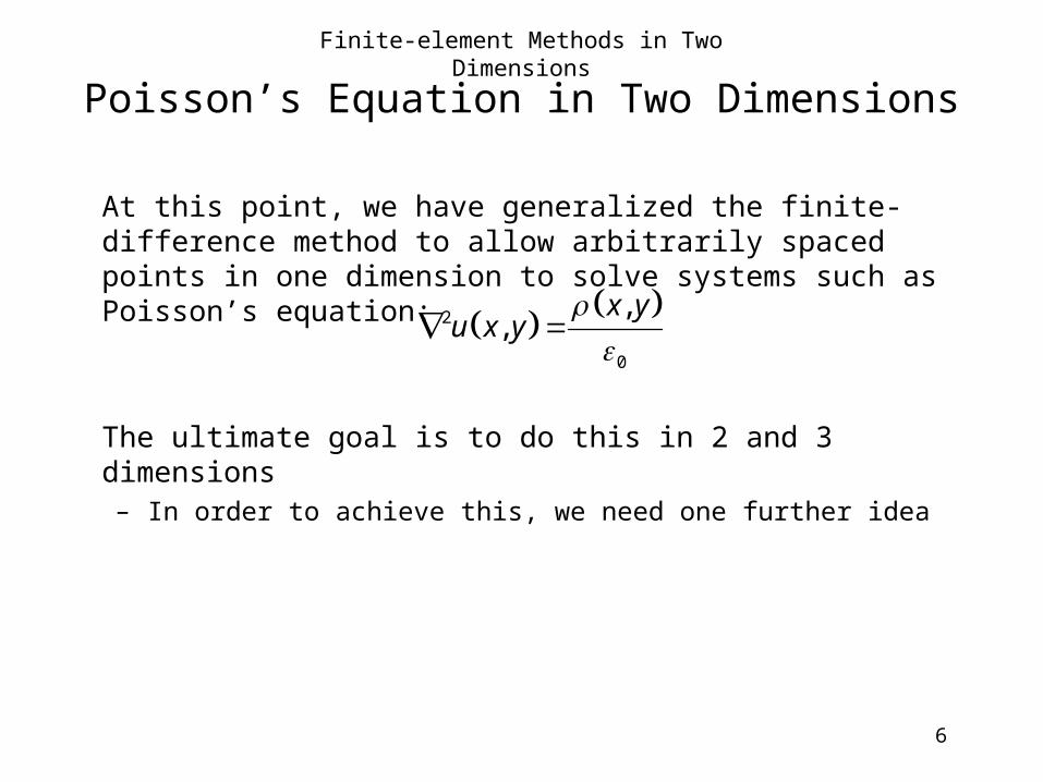
Poisson’s Equation in Two Dimensions
At this point, we have generalized the finite-difference method to allow arbitrarily spaced points in one dimension to solve systems such as Poisson’s equation:
The ultimate goal is to do this in 2 and 3 dimensions– In order to achieve this, we need one further idea
2
0
,,
x yu x y

Finite-element Methods in Two Dimensions
7
Extending Test Functions
In the previous – Use triangles to divide up the region instead of intervals
• Tessellations
– Approximate the solution using interpolating polynomials
Intervals
Tessellation
Finite-element Methods in Two Dimensions
8
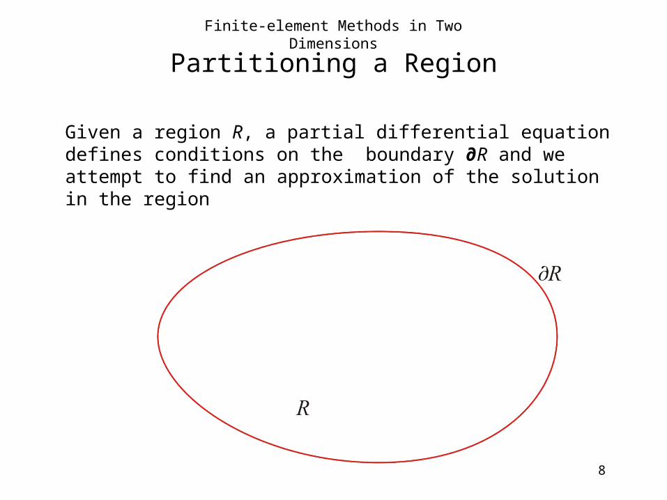
Partitioning a Region
Given a region R, a partial differential equation defines conditions on the boundary ∂R and we attempt to find an approximation of the solution in the region

Finite-element Methods in Two Dimensions
9
Partitioning a Region
We have seen how using finite differences, we:– Create a uniform grid
– Assign points to either the boundary or the interior of the region

Finite-element Methods in Two Dimensions
10
Partitioning a Region
Unfortunately, uniform grids make a poor approximation of most real-world situations

Finite-element Methods in Two Dimensions
11
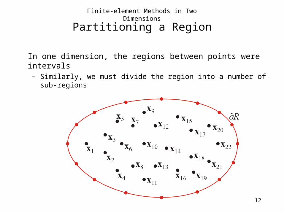
Partitioning a Region
It would be much more desirable to allow the user to select the placement of points where appropriate:– Non-linear boundaries can be fitted
– Points can be concentrated at regions of interest
Let N be the number interior points – in this case, 22
Finite-element Methods in Two Dimensions
12
Partitioning a Region
In one dimension, the regions between points were intervals– Similarly, we must divide the region into a number of sub-regions

Finite-element Methods in Two Dimensions
13
Partitioning a Region
Our goal will be to find approximations of the solution on the interior of the region R

Finite-element Methods in Two Dimensions
14
Partitioning a Region
We will divide the region into triangular elements:– This forms a connected graph
– The collection of all triangles is a tessellation
– Tessella is the Latin word for a small piece of a mosaic

Finite-element Methods in Two Dimensions
15
Partitioning a Region
From wikipedia: a tessellation of a 2D magnetostatic configuration
User: Zureks

Finite-element Methods in Two Dimensions
16
Defining Test Functions
In one dimension, for each interiorpoint, xk, we used the two adjacentintervals upon which we definedthe test functions– The support of the test function
6(x) is the interval [x5, x7]
6(x)
7(x)

Finite-element Methods in Two Dimensions
17
Defining Test Functions
In two dimensions, given the point xk, we will define a test function on the region comprised of triangles adjacent to xk
– Call that region Rk

Finite-element Methods in Two Dimensions
18
Defining Test Functions
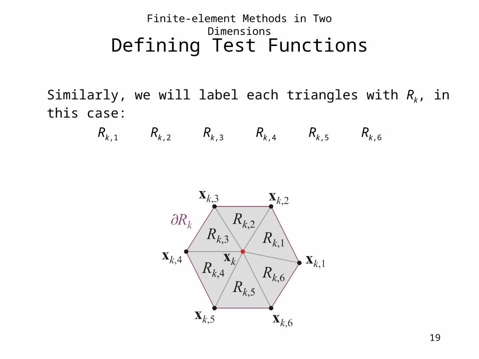
For ease of reference, given a point xk, we will number the adjacent points, in this case:
xk,1 xk,2 xk,3 xk,4 xk,5 xk,6
Finite-element Methods in Two Dimensions
19
Defining Test Functions
Similarly, we will label each triangles with Rk, in this case:
Rk,1 Rk,2 Rk,3 Rk,4 Rk,5 Rk,6

Finite-element Methods in Two Dimensions
20
Defining Test Functions
On each region Rk, we will define a piecewise planar test function
– The test function is k(x, y)
– It is defined to be zero outside Rk
– It is also useful to have it zero on the boundary ∂Rk

Finite-element Methods in Two Dimensions
21
Defining Test Functions
The formula for each plane k, ℓ(x, y) defined on Rk, ℓ is a plane of the form x + y + – To find it, we use linear algebra

Finite-element Methods in Two Dimensions
22
Finding Interpolating Planes
Given three points in the plane
(x1, y1), (x2, y2), (x3, y3)
if we want to find the interpolating plane x + y + that passes through these points z1, z2, and z3, respectively, we must solve the system of linear equations
1 1 1
2 2 2
3 3 3
x y z
x y z
x y z

Finite-element Methods in Two Dimensions
23
Finding Interpolating Planes
Rewritten using matrices and vectors, we must solve:
1 1 1
2 2 2
3 3 3
1
1
1
x y z
x y z
x y z

Finite-element Methods in Two Dimensions
24
Finding Interpolating Planes
Example, given the points in the plane
(1.3, 5.4), (2.9, 7.0) and (6.5, 4.9)

Finite-element Methods in Two Dimensions
25
Finding Interpolating Planes
Example, given the points in the plane
(1.3, 5.4), (2.9, 7.0) and (6.5, 4.9)
we want to find the polynomial x + y + that passes through the points 2.8, 1.6 and 3.9, respectively

Finite-element Methods in Two Dimensions
26
Finding Interpolating Planes
Example, given the points in the plane
(1.3, 5.4), (2.9, 7.0) and (6.5, 4.9)
we want to find the polynomial x + y + that passes through the points 2.8, 1.6 and 3.9, respectively
We must therefore solve
>> [1.3 5.4 1; 2.9 7.0 1; 6.5 4.9 1] \ [2.8 1.6 3.9]'ans = 0.1272 -0.8772 7.3715
1.3 5.4 1 2.8
2.9 7.0 1 1.6
6.5 4.9 1 3.9

Finite-element Methods in Two Dimensions
27
Finding Interpolating Planes
From>> [1.3 5.4 1; 2.9 7.0 1; 6.5 4.9 1] \ [2.8 1.6 3.9]'ans = 0.1272 -0.8772 7.3715
we have that the interpolating plane is
0.1272x – 0.8772y + 7.3715

Finite-element Methods in Two Dimensions
28
Using the Test Function
Now, going back to the problem:– We have the test function k(x, y) and we have a function V(x, y) that is
known to satisfy the formula
V(x, y) = 0
As we did in one dimension, it must therefore be true that
, , 0k
k
R
x y V x y dxdy

Finite-element Methods in Two Dimensions
29
Using the Test Function
Again, let’s consider Poisson’s equation:
We defined
and thus our integral is
2
0
,, , 0
k
k
R
x yx y u x y dxdy
2
0
,,
x yu x y
2
0
,, ,
def x yV x y u x y

Finite-element Methods in Two Dimensions
30
Using the Test Function
Expanding the integral, we get
where the right-hand side is reasonably easy to calculate
The left-hand side, however, requires furthercalculus
2
0
,, , ,
k k
k k
R R
x yx y u x y dxdy x y dxdy

Finite-element Methods in Two Dimensions
31
Using the Test Function
Using the 2-dimensional equivalent of integration-by-parts, we get:
2, , , , , ,k k k
k k k
R R R
x y u x y dxdy x y u x y d x y u x y dxdy
s

Finite-element Methods in Two Dimensions
32
Using the Test Function
Using the 2-dimensional equivalent of the fundamental theorem of calculus:
However, recall that we specifically chose a test function that is zero on the boundary ∂Rk
– Therefore, the first term disappears!
2, , , , , ,k k k
k k k
R R R
x y u x y dxdy x y u x y d x y u x y dxdy
s
0

Finite-element Methods in Two Dimensions
33
Using the Test Function
Therefore, we have the easier integral:
and therefore we have
2, , , ,k k
k k
R R
x y u x y dxdy x y u x y dxdy
0
,, , ,
k k
k k
R R
x yx y u x y dxdy x y dxdy

Finite-element Methods in Two Dimensions
34
Using the Test Function
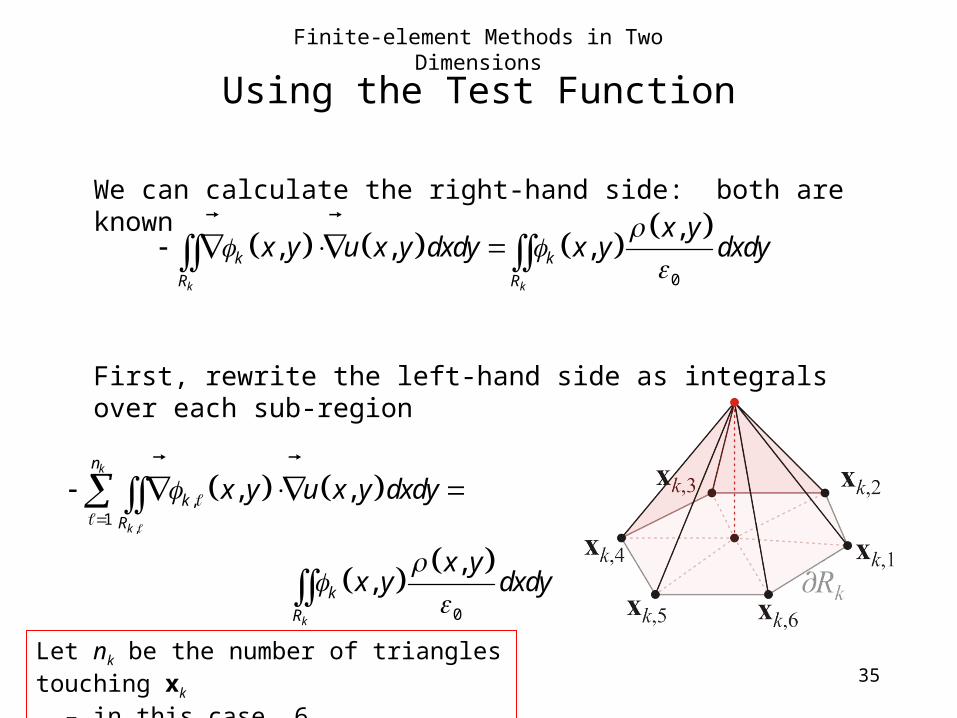
We can calculate the right-hand side: both are known
The left-hand side has the unknown function u(x, y)…
0
,, , ,
k k
k k
R R
x yx y u x y dxdy x y dxdy
Finite-element Methods in Two Dimensions
35
Using the Test Function
We can calculate the right-hand side: both are known
First, rewrite the left-hand side as integrals over each sub-region
0
,, , ,
k k
k k
R R
x yx y u x y dxdy x y dxdy
,
,1
0
, ,
,,
k
k
k
n
k
R
k
R
x y u x y dxdy
x yx y dxdy
Let nk be the number of triangles touching xk
– in this case, 6

Finite-element Methods in Two Dimensions
36
Finding the Test Function Gradient
The test function defined on each sub-region is planar, that is
thus we can easily calculate:
,
,
,
,
,,
k
k
k
x yx
x yx y
y
, ,k x y x y
,
,1
0
, ,
,,
k
k
k
n
k
R
k
R
x y u x y dxdy
x yx y dxdy

Finite-element Methods in Two Dimensions
37
Finding the Test Function Gradient
To find the gradient of this plane, we must find the vector
,
,1
0
, ,
,,
k
k
k
n
k
R
k
R
x y u x y dxdy
x yx y dxdy
1 1
,1 2 2
,2 3 3
: 1 1
: 1 0
: 1 0
k
k
k
x y
x y
x y
x
x
x
Finite-element Methods in Two Dimensions
38
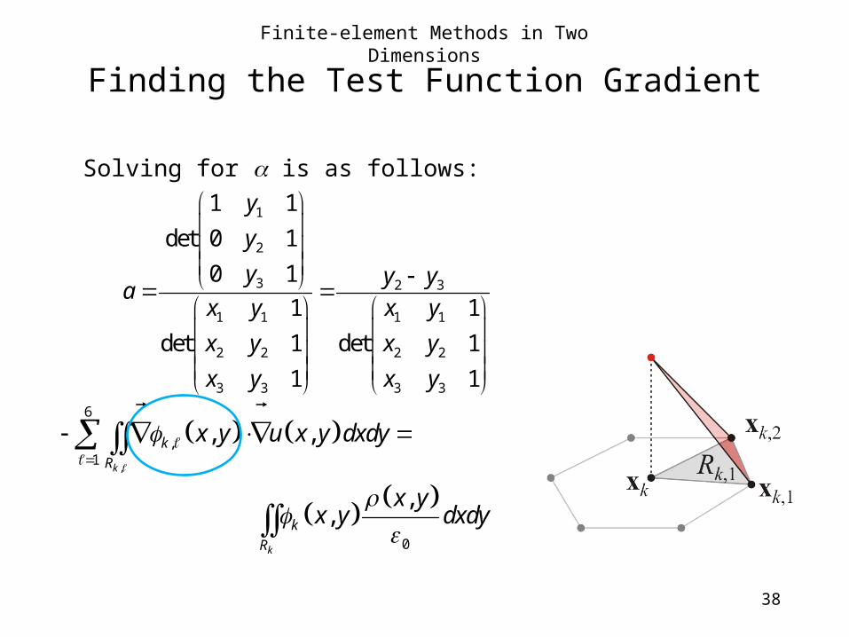
Finding the Test Function Gradient
Solving for is as follows:
,
6
,1
0
, ,
,,
k
k
k
R
k
R
x y u x y dxdy
x yx y dxdy
1
2
3 2 3
1 1 1 1
2 2 2 2
3 3 3 3
1 1
det 0 1
0 1
1 1
det 1 det 1
1 1
y
y
y y ya
x y x y
x y x y
x y x y

Finite-element Methods in Two Dimensions
39
Finding the Test Function Gradient
Solving for is as follows:
,
6
,1
0
, ,
,,
k
k
k
R
k
R
x y u x y dxdy
x yx y dxdy
1
2
3 3 2
1 1 1 1
2 2 2 2
3 3 3 3
1 1
det 0 1
0 1
1 1
det 1 det 1
1 1
x
x
x x xx y x y
x y x y
x y x y

Finite-element Methods in Two Dimensions
40
Approximating the Solution Gradient
The next step is to approximate the unknown
,
6
,1
0
, ,
,,
k
k
k
R
k
R
x y u x y dxdy
x yx y dxdy
,u x y

Finite-element Methods in Two Dimensions
41
Approximating the Solution Gradient
The actual unknown function u(x, y) an unknown and likely non-linear function– You don’t get paid $100 000/a to find a linear function…

Finite-element Methods in Two Dimensions
42
Approximating the Solution Gradient
Recall from 1-D finite element methods:– We approximated the solution with an unknown piecewise
linear function

Finite-element Methods in Two Dimensions
43
Approximating the Solution Gradient
We are attempting to approximate u(x, y) at a number of interior points where the solution is defined on the border

Finite-element Methods in Two Dimensions
44
Approximating the Solution Gradient
We can do the same as we did in one dimension:– Approximate the solution by a piecewise planer approximation

Finite-element Methods in Two Dimensions
45
Approximating the Solution Gradient
As before, we can find the interpolating polynomial:
,
6
,1
0
, ,
,,
k
k
k
R
k
R
x y u x y dxdy
x yx y dxdy
1 1
,1 2 2 ,1
,2 3 3 ,2
: 1
: 1
: 1
k k
k k
k k
x y a u
x y b u
x y c u
x
x
x

Finite-element Methods in Two Dimensions
46
Approximating the Solution Gradient
To find the gradient of this triangle, we must find the vector
,
6
,1
0
, ,
,,
k
k
k
R
k
R
x y u x y dxdy
x yx y dxdy
1 1
,1 2 2 ,1
,2 3 3 ,2
: 1
: 1
: 1
k k
k k
k k
x y a u
x y b u
x y c u
x
x
x
a
b

Finite-element Methods in Two Dimensions
47
Approximating the Solution Gradient
Solving for a is as follows:
,
6
,1
0
, ,
,,
k
k
k
R
k
R
x y u x y dxdy
x yx y dxdy
1
,1 2
,2 3 2 1 ,2 ,1 3 3 1 ,1 2 ,2
1 1 1 1
2 2 2 2
3 3 3 3
1
det 1
1
1 1
det 1 det 1
1 1
k
k
k k k k k k k
u y
u y
u y u y y u u y u y y u y ua
x y x y
x y x y
x y x y

Finite-element Methods in Two Dimensions
48
Approximating the Solution Gradient
Solving for b is as follows:
,
6
,1
0
, ,
,,
k
k
k
R
k
R
x y u x y dxdy
x yx y dxdy
1
2 ,1
3 ,2 1 ,1 3 2 ,2 1 ,2 2 ,1 3
1 1 1 1
2 2 2 2
3 3 3 3
1
det 1
1
1 1
det 1 det 1
1 1
k
k
k k k k k k k
x u
x u
x u x u x u x u x u u x u xb
x y x y
x y x y
x y x y

Finite-element Methods in Two Dimensions
49
Approximating the Double Integral
Thus, we can find both gradients:
If you look back, all values are either known– The positions of the points xk, xk,1 and xk,2:
x1, x2, x3, y1, y2 , y3
or unknown constants uk, uk,1 and uk,2 :
– Take them out of the integral
,1 ,1
, , , ,k k
k
R R
ax y u x y dxdy dxdy
b
,1
1kR
a b dxdy

Finite-element Methods in Two Dimensions
50
Approximating the Double Integral
Finally, we note that the right-hand integral
is just the area of the region Rk,1, call it Ak,1:
,1 ,1
, , , 1k k
k
R R
x y u x y dxdy a b dxdy
1 1
,1 2 2
3 3
11
det 12
1k
x y
A x y
x y

Finite-element Methods in Two Dimensions
51
Approximating the Double Integral
Thus, for each interior point xk, we must calculate:
For each xk, there are nk adjacent triangles Rk,ℓ, and each of these is associated given three points, call them
x1 = (x1, y1), x2 = (x2, y2), x3 = (x3, y3)
and the unknowns associated with, call them u1, u2 and u3:
– Each interior point ends up with nk linear equations that are summed together forming a single linear equation
, ,
, ,1 1 0
,, , ,
k k
k k
n n
k k
R R
x yx y u x y dxdy x y dxdy

Finite-element Methods in Two Dimensions
52
Approximating the Double Integral
If the ratio is a constant, the right-hand integral can be
simplified further:
where Ak is the area of the region Rk
,
,1 0
, 1,
3
k
k
n
k k
R
x yx y dxdy A
0
,x y

Finite-element Methods in Two Dimensions
53
Finding the points
This will produce N linear equations and unknowns– We can solve this system of linear equations for the unknown values
u1, u2, u3, …, uN

Finite-element Methods in Two Dimensions
54
Code For 2-D Finite Elements
A set of functions are available on the web site that set a finite element system and solve for the interior values– It assumes the right-hand side of Poisson’s equation is constant
2 ,u x y
fe_system( rho, pts )
Create a data structure for the above equation by passing in a set of points (interior and boundary) with values for the boundary points and -Inf for the interior points
fe_update( obj, pt, alist )
Indicate the tessellation around an interior point by passing a list of neighbouring points
fe_solve( obj )
Having called fe_update for each interior point, now solve the system of equations returning the initial argument pts with all values -Inf replaced with values
fe_coeffs( x1, x2, x3 ) A helper function

Finite-element Methods in Two Dimensions
55
Example 1
Consider the following region and we are trying to approximate Laplace’s equation ( = 0) with the following region and boundary values:

Finite-element Methods in Two Dimensions
56
Example 1
We can define the system as follows:pts1 = [ 0 -1 -1 % 1 -1 0 1 % 2 0 0 -Inf % 3 1 0 1 % 4 -1 1 0 % 5 0 1 -Inf % 6 0 2 -4]'; % 7obj1 = fe_system( 0, pts1 );
Finite-element Methods in Two Dimensions
57
Example 1
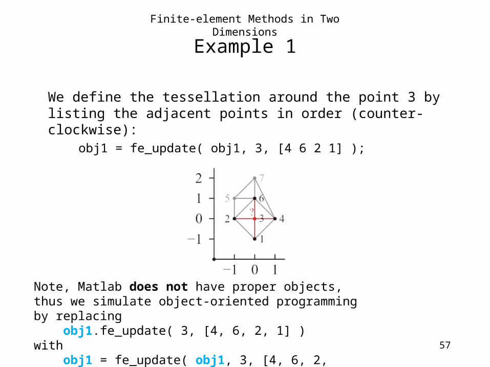
We define the tessellation around the point 3 by listing the adjacent points in order (counter-clockwise):
obj1 = fe_update( obj1, 3, [4 6 2 1] );
Note, Matlab does not have proper objects, thus we simulate object-oriented programming by replacing obj1.fe_update( 3, [4, 6, 2, 1] )with obj1 = fe_update( obj1, 3, [4, 6, 2, 1] )

Finite-element Methods in Two Dimensions
58
Example 1
Similarly, we define the tessellation around the point 6 by listing the adjacent points in order (counter-clockwise):
obj1 = fe_update( obj1, 6, [4 7 5 2 3] );
Finite-element Methods in Two Dimensions
59
Example 1
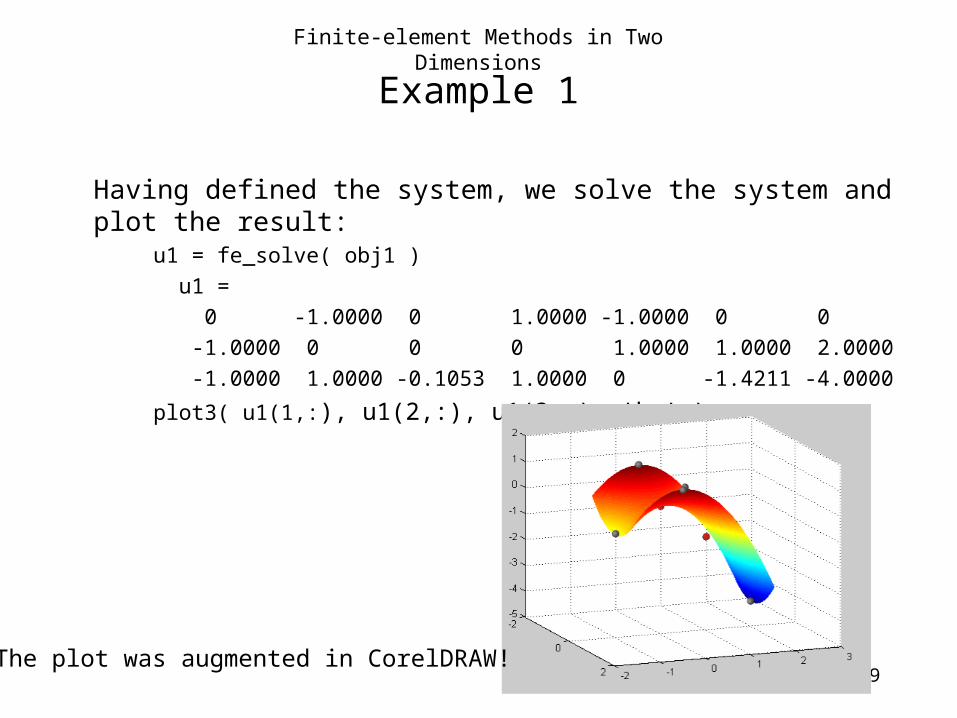
Having defined the system, we solve the system and plot the result:u1 = fe_solve( obj1 ) u1 = 0 -1.0000 0 1.0000 -1.0000 0 0 -1.0000 0 0 0 1.0000 1.0000 2.0000 -1.0000 1.0000 -0.1053 1.0000 0 -1.4211 -4.0000
plot3( u1(1,:), u1(2,:), u1(3,:), 'ko' )
The plot was augmented in CorelDRAW!

Finite-element Methods in Two Dimensions
60
Example 2
Consider the following region and we are trying to approximate Poisson’s equation with = 4, the following region and boundary values:

Finite-element Methods in Two Dimensions
61
Example 2
We can define the system as follows:pts2 = [-2 -2 8 % 1 1 -2 5 % 2 -3 -1 10 % 3 0 -1 -Inf % 4 3 -1 10 % 5 -1 0 -Inf % 6 2 0 -Inf % 7 -3 1 10 % 8 1 1 –Inf % 9 3 1 10 % 10 -2 2 8 % 11 0 2 -Inf % 12 1 3 10]'; % 13obj2 = fe_system( 4, pts2 );

Finite-element Methods in Two Dimensions
62
Example 2
We then define the various tessellations:obj2 = fe_update( obj2, 4, [1 2 7 9 6] );obj2 = fe_update( obj2, 6, [1 4 9 12 11 8 3] );obj2 = fe_update( obj2, 7, [2 5 10 9 4] );obj2 = fe_update( obj2, 9, [4 7 10 13 12 6] );obj2 = fe_update( obj2, 12, [6 9 13 11] );

Finite-element Methods in Two Dimensions
63
Example 2
Finally, we solve the system:u2 = fe_solve( obj2 ) u = Columns 1 through 8 -2.0000 1.0000 -3.0000 0 3.0000 -1.0000 2.0000 -
3.0000 -2.0000 -2.0000 -1.0000 -1.0000 -1.0000 0 0
1.0000 8.0000 5.0000 10.0000 1.8256 10.0000 1.2883 4.6679
10.0000
Columns 9 through 13 1.0000 3.0000 -2.0000 0 1.0000 1.0000 1.0000 2.0000 2.0000 3.0000 2.9111 10.0000 8.0000 5.5663 10.0000
plot3( u2(1,:), u2(2,:), u2(3,:), 'o' )

Finite-element Methods in Two Dimensions
64
Example 2
Here we see the boundary points and the actual solution (light blue) and the approximations (in red)

Finite-element Methods in Two Dimensions
65
Summary
This topic discusses an introduction to finite-element methods in two dimensions– We generalized the test functions in one dimension
– Created a tessellation of the region R
– Defined planar test functions• Found the gradient of the planes making the test functions
– Approximated the solution with piecewise planar sections
– Created a linear equation• This is done for each interior point
– The resulting system of linear equations may be solved
– Two examples…

Finite-element Methods in Two Dimensions
66
What’s Next?
The next step is to go to three dimensions– Divide the region into tetrahedral regions
– 3-dimensional tessellations
Tessellation User: Tom Ruen
Robert Webb's Great Stella softwarehttp://www.software3d.com/Stella.html

Finite-element Methods in Two Dimensions
67
References
[1] Glyn James, Advanced Modern Engineering Mathematics, 4th Ed., Prentice Hall, 2011, §§9.2-3.

Finite-element Methods in Two Dimensions
68
Usage Notes
• These slides are made publicly available on the web for anyone to use
• If you choose to use them, or a part thereof, for a course at another institution, I ask only three things:
– that you inform me that you are using the slides,– that you acknowledge my work, and– that you alert me of any mistakes which I made or changes which you make, and
allow me the option of incorporating such changes (with an acknowledgment) in my set of slides
Sincerely,
Douglas Wilhelm Harder, MMath
Related Documents