Math 19a: Modeling and Differential Equations for the Life Sciences Calculus Review Danny Kramer Fall 2013.

Math 19a: Modeling and Differential Equations for the Life Sciences

Calculus Review

Danny KramerFall 2013

Derivatives

Point Slope Concept

𝑓 ′ (𝑥 )= lim∆𝑥→ 0

𝑓 (𝑥+∆ 𝑥 )− 𝑓 (𝑥)∆ 𝑥

𝑑𝑑𝑥

𝑓 (𝑥 )=𝑠𝑙𝑜𝑝𝑒𝑎𝑡 𝑎𝑛𝑦 𝑝𝑜𝑖𝑛𝑡 𝑥

Think of , but change in y measured over infinitely small change in x

x

y

Solve it Out

Derivate of x2?

0

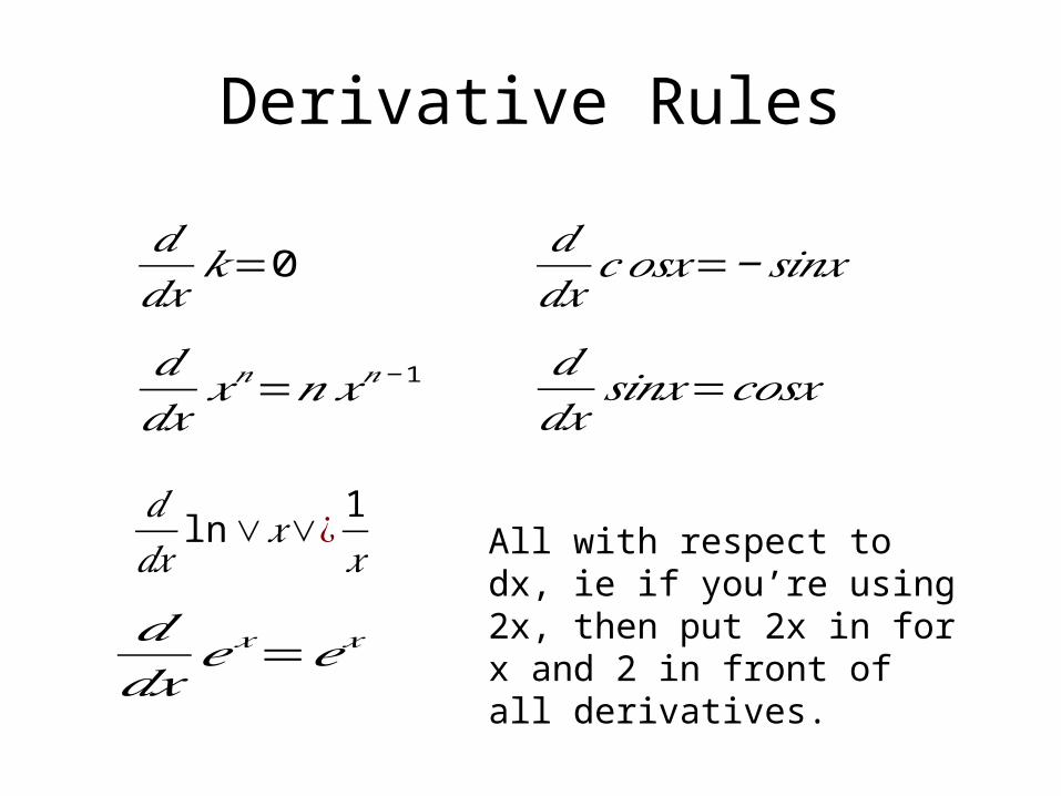
Derivative Rules

𝑑𝑑𝑥

𝑘=0

𝑑𝑑𝑥

𝑥𝑛=𝑛𝑥𝑛−1

𝑑𝑑𝑥

𝑐 𝑜𝑠𝑥=−𝑠𝑖𝑛𝑥

𝑑𝑑𝑥

𝑠𝑖𝑛𝑥=𝑐𝑜𝑠𝑥

𝑑𝑑𝑥ln ∨𝑥∨¿

1𝑥

𝑑𝑑𝑥

𝑒𝑥=𝑒𝑥

All with respect to dx, ie if you’re using 2x, then put 2x in for x and 2 in front of all derivatives.

Derivatives and Operations

𝑑𝑑𝑥

( 𝑓 +𝑔)= 𝑓 ′+𝑔 ′

𝑑𝑑𝑥

( 𝑓 −𝑔)= 𝑓 ′−𝑔 ′

𝑑𝑑𝑥

( 𝑓 ∗𝑔)= 𝑓 ′𝑔+ 𝑓𝑔 ′

𝑑𝑑𝑥

¿

𝑁𝑜𝑡𝑒 :𝑑𝑑𝑥

𝑓= 𝑓 ′

Applications

• Position• Speed/Velocity• Acceleration

𝑣=∆𝑥∆ 𝑡

a=∆ 𝑣∆ 𝑡

𝑣 (𝑡 )= 𝑑𝑑𝑡

𝑥=𝑥 ′ (t)

a (t )= 𝑑𝑑𝑡

𝑣= 𝑑𝑑𝑡 ( 𝑑𝑑𝑡 𝑥)= 𝑑2

𝑑𝑡 2𝑥=𝑥 ′ ′ (𝑡)

Maxima and Minima

x

f(x)

f’(x)=0

f’(x)=0

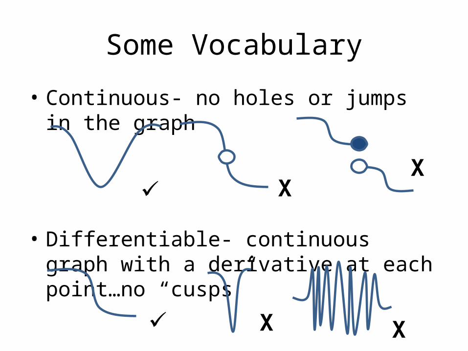
Some Vocabulary

• Continuous- no holes or jumps in the graph

• Differentiable- continuous graph with a derivative at each point…no “cusps”

✓ XX

✓ X X

Sample Problem

Maximum Point?

Integrals and Antiderivatives

Area Concept

𝐷𝑒𝑟𝑖𝑣𝑎𝑡𝑖𝑣𝑒→∆𝑞𝑢𝑎𝑛𝑡𝑖𝑡𝑦∆ 𝑡𝑖𝑚𝑒

=𝑟𝑎𝑡𝑒

It is area under a curve, but think of it more generally as multiplying a changing rate by the elapsed time over which the rate occurs, giving you the change in quantity that the rate is measuring.

x

y

=

Some Notation

∫ 𝑓 (𝑥 )=𝐹 (𝑥)𝐹 ′ (𝑥 )= 𝑓 (𝑥)

Antiderivative Rules and Operations

What’s with the C? Disappears in derivative!

∫𝑒𝑥=𝑒𝑥+𝐶∫𝑐𝑜𝑠𝑥=𝑠𝑖𝑛𝑥+𝐶∫ 𝑠𝑖𝑛𝑥=−𝑐𝑜𝑠𝑥+𝐶

∫( 𝑓 +𝑔)=∫ 𝑓 +∫𝑔 ∫( 𝑓 −𝑔)=∫ 𝑓 −∫𝑔

U substitution

Replace to visualize

∫𝑒sin ( 𝑥)cos (𝑥)𝑑𝑥→∫𝑒u𝑑𝑢=𝑒𝑢+𝐶→𝑢=sin (𝑥)𝑑𝑢=cos (𝑥)𝑑𝑥

𝑒𝑠𝑖𝑛𝑥+𝐶

Integration by Parts

∫𝑢𝑑𝑣=𝑢𝑣−∫𝑣𝑑𝑢 Opposite of product rule. Test it out!

What Becomes u?LogInverse Trig (the arcs)AlgebraTrigExponential

∫𝑥 𝑒−𝑥𝑑𝑥𝑢=𝑥𝑑𝑢=𝑑𝑥𝑣=−𝑒−𝑥𝑑𝑣=𝑒−𝑥𝑑𝑥

Taylor Series

Approximating Polynomial Curves

x

f(x)

x = a

f(a)

Taylor’s Formula

𝑓 (𝑥 )= 𝑓 (𝑎)+ 𝑓 ′ (𝑎 ) (𝑥−𝑎 )+ 𝑓 ′ ′ (𝑎)2 !

(𝑥−𝑎)2+…

𝑇=∑𝑛=0

∞ 𝑓 𝑛(𝑎)𝑛 !

(𝑥−𝑎 )𝑛

Practicing Taylor

𝑓 (𝑥 )=𝑥 𝑒−𝑥

𝑓 ′ (𝑥 )=𝑒−𝑥−𝑥 𝑒−𝑥=𝑒−𝑥(1−x )

𝑓 ′ ′ (𝑥 )=−𝑒−𝑥−𝑒−𝑥 (1− x )=𝑒−𝑥(x−2)

Practicing Taylor

𝑓 (1 )=(1 )𝑒−1=𝟏𝒆

=

𝑓 ′ ′ (1 )=−𝑒−1−𝑒−1 (1−1 )=𝑒−1 (1−2 )=−𝟏𝒆

𝑇= 𝑓 (𝑎 )+ 𝑓 ′ (𝑎) (𝑥−𝑎 )+ 𝑓 ′ ′(𝑎)2 !

(𝑥−𝑎)2 ,𝑎=1

𝑇 𝑥=𝟏𝒆

+𝟎−𝟏2𝒆

(𝑥−1)2

Parametric Curves

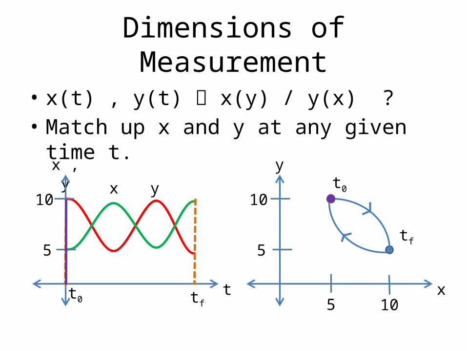
Dimensions of Measurement

• x(t) , y(t) x(y) / y(x) ?• Match up x and y at any given time t.

t

x , yx y

5

10

x

y

5

10

5 10t0 tf

t0

tf

Parametric Conversion

𝑥=2 𝑡+1 𝑦=3 𝑡−1

𝑡=𝑥−12

𝑡=𝑦+13

𝑥−12

=𝑦+13

𝑦+1=32(𝑥−1)

𝑦=32𝑥−

52→𝑥=

23𝑦+53

𝑑𝑥𝑑𝑡

=2 𝑡𝑑𝑦𝑑𝑡

=3 𝑡

𝑑𝑦𝑑𝑡𝑑𝑥𝑑𝑡

=3 𝑡2𝑡

=3 /2

𝑑𝑦𝑑𝑥

=3/2