MATH 183 The Chi-Square Distributions - WKUpeople.wku.edu/david.neal/183/Unit4/ChiSquare.pdf · Dr. Neal, WKU MATH 183 The Chi-Square Distributions The chi-square distributions can

Dr. Neal, WKU MATH 183 The Chi-Square Distributions The chi-square distributions can be used in statistics to analyze the standard deviation

€

σ of a normally distributed measurement and to test the goodness of fit of various population models on a set of data. A chi-square distribution is based on a parameter known as the degrees of freedom

€

n , where

€

n is an integer greater than or equal to 1. Such a random variable is denoted by X ~ χ2(n) . The χ2(n) distribution is defined to be the sum of the squares of

€

n independent standard normal distributions. For example, suppose X1, . . . , Xn are independent normally distributed measurements having mean µ i and standard deviation σi for i = 1, . . .,

€

n . These measurements could be the heights or IQ scores of various groups of people. By subtracting the mean and then dividing by the standard deviation, we convert each measurement into a standard normal distribution: Zi = Xi − µi

σi ~ N(0, 1) , for

€

1≤ i ≤ n .

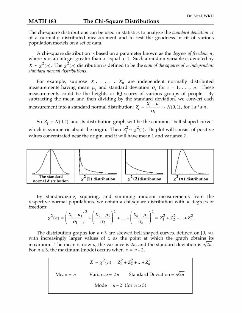
So Z1 ~ N(0, 1) and its distribution graph will be the common “bell-shaped curve” which is symmetric about the origin. Then Z1

2~ χ2(1) . Its plot will consist of positive values concentrated near the origin, and it will have mean 1 and variance 2 .

The standard

normal distribution χ2 (1) distribution χ

2 (2)distribution χ2 (n) distribution

By standardizing, squaring, and summing random measurements from the respective normal populations, we obtain a chi-square distribution with

€

n degrees of freedom:

χ2(n) = X1 − µ1σ1

⎛

⎝ ⎜ ⎜

⎞

⎠ ⎟ ⎟

2+

X2 − µ2σ2

⎛

⎝ ⎜ ⎜

⎞

⎠ ⎟ ⎟

2+ . . . + Xn − µn

σn

⎛

⎝ ⎜ ⎜

⎞

⎠ ⎟ ⎟

2 = Z1

2 + Z22 + .. .+ Zn

2 .

The distribution graphs for

€

n ≥ 3 are skewed bell-shaped curves, defined on [0, ∞), with increasingly larger values of x as the point at which the graph obtains its maximum. The mean is now n, the variance is 2n, and the standard deviation is

€

2n . For

€

n ≥ 3, the maximum (mode) occurs when

€

x =

€

n − 2 .

X ~ χ2(n) = Z12 + Z2

2 + .. .+ Zn2

Mean =

€

n Variance = 2 n Standard Deviation =

€

2n

Mode =

€

n − 2 (for

€

n ≥ 3)

Dr. Neal, WKU The theoretical distribution curve is given by

f (x) = Cn xn / 2−1 e− x /2 , for

€

x ≥ 0, where Cn is a constant that depends on

€

n given by

Cn =

1

2n /2 n2−1⎛

⎝ ⎜

⎞ ⎠ ⎟ !

2(n−2)/2 n − 12

⎛ ⎝ ⎜

⎞ ⎠ ⎟ !

(n −1)! π

⎧

⎨

⎪ ⎪ ⎪ ⎪

⎩

⎪ ⎪ ⎪ ⎪

€

for n even

for n odd .

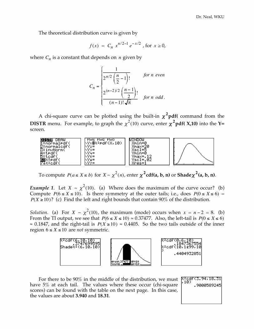
A chi-square curve can be plotted using the built-in χ 2pdf( command from the DISTR menu. For example, to graph the χ2(10) curve, enter χ 2pdf( X,10) into the Y= screen.

To compute P(a ≤ X ≤ b) for X ~ χ2(n) , enter χ 2cdf(a, b, n) or Shadeχ 2(a, b, n). Example 1. Let X ~ χ2(10) . (a) Where does the maximum of the curve occur? (b) Compute P(6 ≤ X ≤ 10) . Is there symmetry at the outer tails; i.e., does P(0 ≤ X ≤ 6) = P(X ≥10)? (c) Find the left and right bounds that contain 90% of the distribution. Solution. (a) For X ~ χ2(10) , the maximum (mode) occurs when x = n − 2 = 8. (b) From the TI output, we see that P(6 ≤ X ≤ 10) ≈ 0.37477. Also, the left-tail is P(0 ≤ X ≤ 6) ≈ 0.1847, and the right-tail is P(X ≥10) ≈ 0.4405. So the two tails outside of the inner region 6 ≤ X ≤10 are not symmetric.

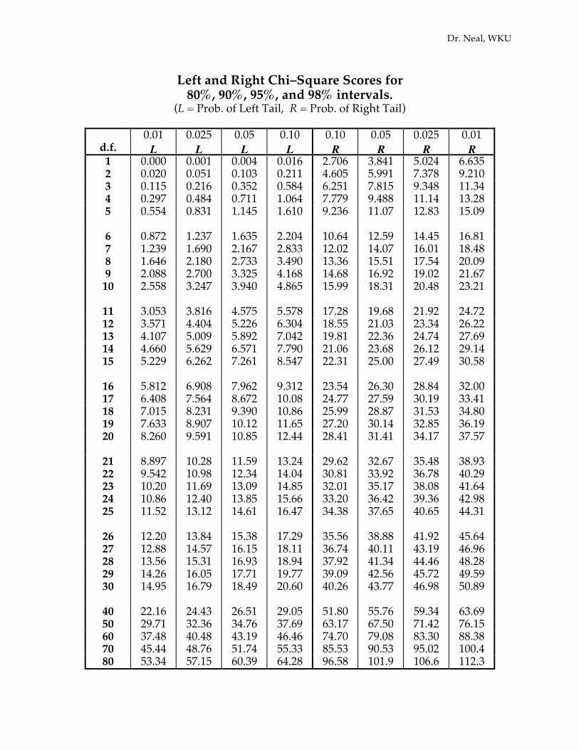
For there to be 90% in the middle of the distribution, we must have 5% at each tail. The values where these occur (chi-square scores) can be found with the table on the next page. In this case, the values are about 3.940 and 18.31.

Dr. Neal, WKU

Left and Right Chi–Square Scores for 80%, 90%, 95%, and 98% intervals.

(L = Prob. of Left Tail, R = Prob. of Right Tail)

0.01 0.025 0.05 0.10 0.10 0.05 0.025 0.01 d.f. L L L L R R R R 1 0.000 0.001 0.004 0.016 2.706 3.841 5.024 6.635 2 0.020 0.051 0.103 0.211 4.605 5.991 7.378 9.210 3 0.115 0.216 0.352 0.584 6.251 7.815 9.348 11.34 4 0.297 0.484 0.711 1.064 7.779 9.488 11.14 13.28 5

0.554 0.831 1.145 1.610 9.236 11.07 12.83 15.09

6 0.872 1.237 1.635 2.204 10.64 12.59 14.45 16.81 7 1.239 1.690 2.167 2.833 12.02 14.07 16.01 18.48 8 1.646 2.180 2.733 3.490 13.36 15.51 17.54 20.09 9 2.088 2.700 3.325 4.168 14.68 16.92 19.02 21.67 10

2.558 3.247 3.940 4.865 15.99 18.31 20.48 23.21

11 3.053 3.816 4.575 5.578 17.28 19.68 21.92 24.72 12 3.571 4.404 5.226 6.304 18.55 21.03 23.34 26.22 13 4.107 5.009 5.892 7.042 19.81 22.36 24.74 27.69 14 4.660 5.629 6.571 7.790 21.06 23.68 26.12 29.14 15

5.229 6.262 7.261 8.547 22.31 25.00 27.49 30.58

16 5.812 6.908 7.962 9.312 23.54 26.30 28.84 32.00 17 6.408 7.564 8.672 10.08 24.77 27.59 30.19 33.41 18 7.015 8.231 9.390 10.86 25.99 28.87 31.53 34.80 19 7.633 8.907 10.12 11.65 27.20 30.14 32.85 36.19 20

8.260 9.591 10.85 12.44 28.41 31.41 34.17 37.57

21 8.897 10.28 11.59 13.24 29.62 32.67 35.48 38.93 22 9.542 10.98 12.34 14.04 30.81 33.92 36.78 40.29 23 10.20 11.69 13.09 14.85 32.01 35.17 38.08 41.64 24 10.86 12.40 13.85 15.66 33.20 36.42 39.36 42.98 25

11.52 13.12 14.61 16.47 34.38 37.65 40.65 44.31

26 12.20 13.84 15.38 17.29 35.56 38.88 41.92 45.64 27 12.88 14.57 16.15 18.11 36.74 40.11 43.19 46.96 28 13.56 15.31 16.93 18.94 37.92 41.34 44.46 48.28 29 14.26 16.05 17.71 19.77 39.09 42.56 45.72 49.59 30

14.95 16.79 18.49 20.60 40.26 43.77 46.98 50.89

40 22.16 24.43 26.51 29.05 51.80 55.76 59.34 63.69 50 29.71 32.36 34.76 37.69 63.17 67.50 71.42 76.15 60 37.48 40.48 43.19 46.46 74.70 79.08 83.30 88.38 70 45.44 48.76 51.74 55.33 85.53 90.53 95.02 100.4 80 53.34 57.15 60.39 64.28 96.58 101.9 106.6 112.3

Dr. Neal, WKU

Theorems I. Let { x1 , x2 , . . . , xn } denote the collection of all random samples of size

€

n from

normally distributed measurements having variance

€

σ 2 . Let

€

S2 = 1n −1

(xi − x )2i=1

n∑ be

the distribution of all possible sample variances. Then

(n −1) S2

σ2 is a χ2(n −1) distribution.

Thus with a normally distributed measurement, we can evaluate P(a ≤ S ≤ b) by

P(a ≤ S ≤ b) = P(a2 ≤ S2 ≤ b2)

= P (n −1)a2

σ 2≤(n −1)S2

σ 2≤(n − 1)b2

σ 2⎛

⎝ ⎜ ⎜

⎞

⎠ ⎟ ⎟

= P (n −1)a2

σ 2≤ χ2 (n −1) ≤ (n −1)b

2

σ2

⎛

⎝ ⎜ ⎜

⎞

⎠ ⎟ ⎟

provided

€

σ 2 is known.

II. Let

€

S2 be the sample variance from a random sample of size

€

n of a normally distributed measurement having variance

€

σ 2 . A confidence interval for

€

σ 2 , with level of confidence r =

€

1−α , is given by

(n −1)S2

R≤ σ 2 ≤

(n −1)S2

L,

where L and R are the left and right bounds of the χ2(n −1) distribution that give r

probability in the middle. A confidence interval for

€

σ is (n −1)S2

R≤ σ ≤

(n −1)S2

L.

III. To test the null hypothesis H0 :

€

σ = M for a normally distributed measurement, we obtain the sample deviation

€

S from a random sample of size

€

n . The test statistic is then

x =(n −1) S2

σ 2=(n − 1) S2

M2 which is compared with the χ2(n −1) distribution. Compute

the (left-tail) P -value P χ2 (n −1) ≤ x( ) for the alternative Ha :

€

σ < M , and compute the

(right-tail) P -value P χ2 (n −1) ≥ x( ) for the alternative Ha :

€

σ > M .

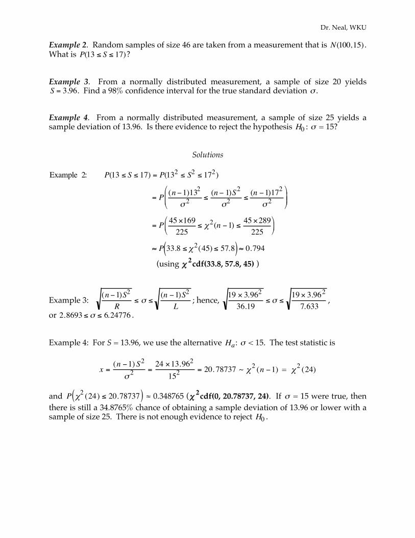
Dr. Neal, WKU Example 2. Random samples of size 46 are taken from a measurement that is N(100,15) . What is P(13 ≤ S ≤ 17)? Example 3. From a normally distributed measurement, a sample of size 20 yields

€

S = 3.96. Find a 98% confidence interval for the true standard deviation

€

σ . Example 4. From a normally distributed measurement, a sample of size 25 yields a sample deviation of 13.96. Is there evidence to reject the hypothesis H0 :

€

σ = 15?

Solutions Example 2: P(13 ≤ S ≤ 17) = P(132 ≤ S2 ≤ 172)

= P (n −1)132

σ 2 ≤(n − 1)S2

σ2 ≤(n −1)172

σ 2

⎛

⎝ ⎜ ⎜

⎞

⎠ ⎟ ⎟

= P 45 ×169225

≤ χ2(n −1) ≤ 45 ×289225

⎛ ⎝ ⎜

⎞ ⎠ ⎟

≈ P 33.8 ≤ χ2(45) ≤ 57.8( ) ≈ 0.794

(using χ 2cdf(33.8, 57.8, 45) )

Example 3: (n −1)S2

R≤ σ ≤

(n −1)S2

L; hence, 19 × 3.962

36.19≤ σ ≤

19 × 3.962

7.633,

or 2.8693 ≤ σ ≤ 6.24776 . Example 4: For S = 13.96, we use the alternative Ha :

€

σ < 15. The test statistic is

x =(n −1) S2

σ 2=24 ×13.962

152= 20. 78737 ~ χ2 (n −1) = χ2 (24)

and P χ2 (24) ≤ 20.78737( ) ≈ 0.348765 (χ 2cdf(0, 20.78737, 24). If

€

σ = 15 were true, then there is still a 34.8765% chance of obtaining a sample deviation of 13.96 or lower with a sample of size 25. There is not enough evidence to reject H0 .

Dr. Neal, WKU

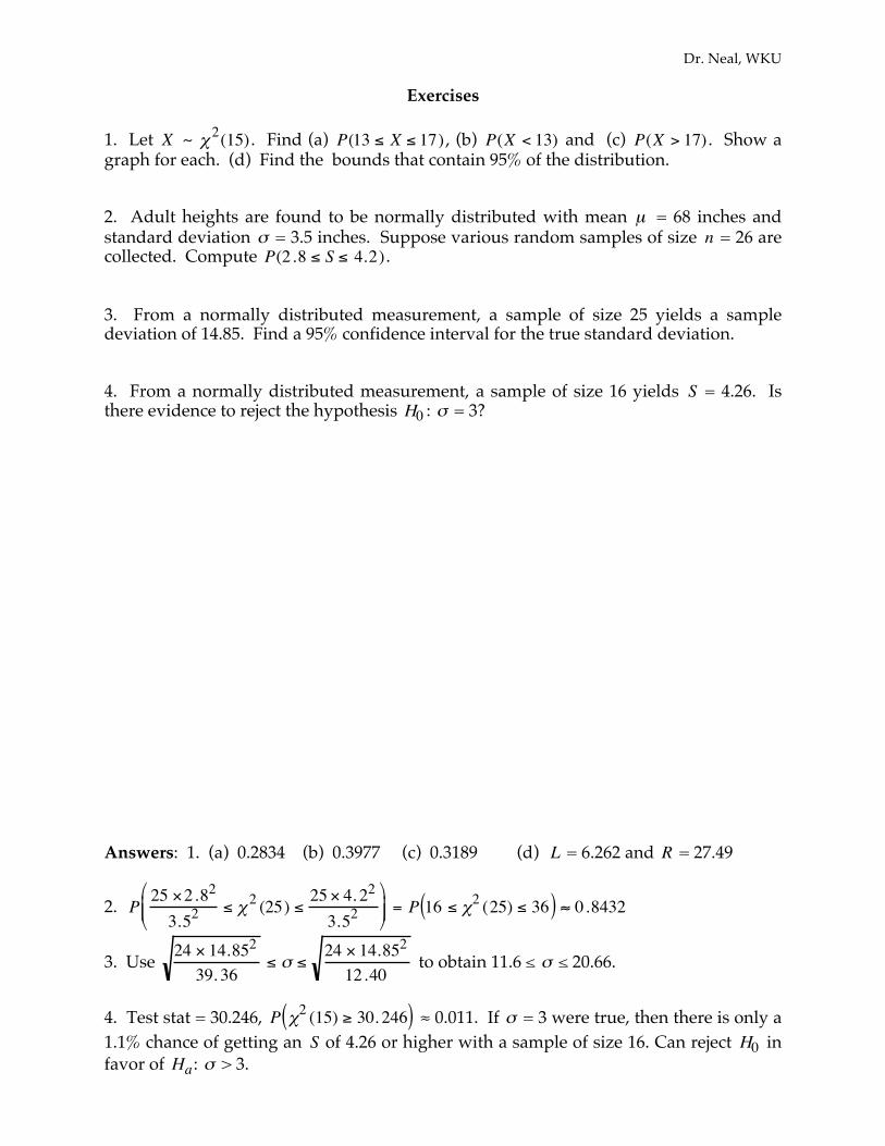
Exercises 1. Let X ~ χ2(15) . Find (a) P(13 ≤ X ≤ 17) , (b) P(X < 13) and (c) P(X > 17) . Show a graph for each. (d) Find the bounds that contain 95% of the distribution. 2. Adult heights are found to be normally distributed with mean µ = 68 inches and standard deviation

€

σ = 3.5 inches. Suppose various random samples of size

€

n = 26 are collected. Compute P(2.8 ≤ S ≤ 4.2) . 3. From a normally distributed measurement, a sample of size 25 yields a sample deviation of 14.85. Find a 95% confidence interval for the true standard deviation. 4. From a normally distributed measurement, a sample of size 16 yields

€

S = 4.26. Is there evidence to reject the hypothesis H0 :

€

σ = 3? Answers: 1. (a) 0.2834 (b) 0.3977 (c) 0.3189 (d) L = 6.262 and R = 27.49

2. P 25 ×2.82

3.52≤ χ2 (25) ≤ 25 × 4. 2

2

3.52⎛

⎝ ⎜ ⎜

⎞

⎠ ⎟ ⎟ = P 16 ≤ χ2 (25) ≤ 36( ) ≈ 0.8432

3. Use 24 × 14.852

39. 36≤ σ ≤

24 × 14.852

12.40 to obtain 11.6 ≤

€

σ ≤ 20.66.

4. Test stat = 30.246, P χ2 (15) ≥ 30. 246( ) ≈ 0.011. If

€

σ = 3 were true, then there is only a 1.1% chance of getting an

€

S of 4.26 or higher with a sample of size 16. Can reject H0 in favor of Ha :

€

σ > 3.