Materials Prices and Productivity - SSCCssc.wisc.edu/~eatalay/materials_prod.pdfmaterial inputs. Using plant-level ... do with plants™technical e¢ ciencies. ... His analysis focuses

Materials Prices and Productivity

Enghin Atalay ∗

March 22, 2013

Abstract

There is substantial within-industry variation in the prices that plants pay for their

material inputs. Using plant-level data from the U.S. Census Bureau, I explore the

consequences and sources of this variation in materials prices. For a sample of in-

dustries with relatively homogeneous products, the standard deviation of plant-level

productivity would be 7% smaller if all plants faced the same materials prices. More-

over, plant-level materials prices are persistent, spatially correlated, and positively

associated with the probability of exit. The contribution of entry and exit to ag-

gregate productivity growth is smaller for productivity measures that are purged of

materials price variation. After documenting these patterns, I discuss three potential

sources of materials price variation: geography, differences in suppliers’marginal costs,

and within-supplier markup differences. Together, these variables explain 15% of the

variation of materials prices.

1 Introduction

There is substantial within-industry variation in the prices that establishments pay for

their material inputs, even in industries that use and produce homogeneous inputs and

outputs. This paper assesses the implications and sources of this variation in materials

prices. When input prices differ across plants, plants may have lower marginal costs not

only because they are able to produce more effi ciently, but also because they are able to

purchase intermediate inputs at relatively low prices.∗I thank Frank Limehouse and Arnie Reznek, for help with the data disclosure process. In addition, I am

indebted to Aditya Bhave, Thomas Chaney, Ali Hortaçsu, Sam Kortum, Ezra Oberfield, Marshall Steinbaum,Nancy Stokey, Chad Syverson, Kirk White, Stephane Wolton, Fabrizio Zilibotti, and five anonymous refereesfor their helpful comments on earlier drafts. Disclaimer: Any opinions and conclusions expressed herein arethose of the author and do not necessarily represent the views of the U.S. Census Bureau. All results havebeen reviewed to ensure that no confidential information is disclosed.

1

Accounting for the variation in materials prices1 provides new answers to two long-

standing questions: First, why are within-industry differences in plants’measured productiv-

ities so large? Second, what is the role of reallocation– via the entry of relatively productive

plants and the exit of unproductive plants– on industry productivity growth?

Large, persistent, within-industry productivity differences are ubiquitous. Syverson

(2004a), for example, estimates that, in the average 4-digit manufacturing industry, the 90th

percentile plant has a total factor productivity that is approximately 90% higher than the

10th percentile plant. Given the importance that a plant’s productivity has for its growth

and survival, as well as the strong relationship between countries’GDPs and the average

productivities of their firms, several papers have tried to explain why some plants are pro-

ductive while others are not. This literature has argued that relatively productive plants

are more likely to: employ high-quality inputs ( Fox and Smeets 2011), patent (Balasub-

ramanian and Sivadasan 2011), enter export or import markets (Bernard and Jensen 1999;

Eslava et al. 2004, 2013), and follow best-practice management techniques (Bloom and Van

Reenen 2010). In addition, productivity dispersion is larger in markets with less intense

competition (Syverson 2004b) and in countries with larger factor misallocations (Hsieh and

Klenow 2009).

In the cited studies, plants’ productivities are calculated as the ratio of outputs

to inputs. Usually, data on input and output prices are not collected, meaning that–

in most cases– real revenues are the measure of establishment outputs, while real input

expenditures are the measure of establishment inputs.2 With these productivity measures,

an establishment’s measured productivity will depend on conditions in output and factor

markets. Potentially, an establishment’s measured productivity could have no relationship

with how effi cient it is in transforming inputs into outputs.

The potential confounding effects of input and output price variation in productivity

estimation are already well known. Both Katayama, Lu, and Tybout (2009) and Gorod-

nichenko (2010) argue, in detail, why plant-level measured productivities may have little to

do with plants’technical effi ciencies. These papers propose structural estimators of estab-

1Throughout this paper, I will use the terms "intermediate inputs" and "materials" interchangeably.2Four partial exceptions are Syverson (2004b), Eslava et al. (2004, 2013), and Ornaghi (2006). Syverson

(2004b) utilizes establishment-level output price data, but does not use establishment-level intermediateinput price data. Ornaghi (2006), on the other hand, has data on materials prices. His analysis focuses onthe estimation of input elasticities, instead of the distribution of plant-level productivities, which is the focushere. Perhaps closest to the current paper, Eslava et al. (2004, 2013) use plant-level input and output pricedata from Colombia to test the hypothesis that a trade liberalization stiffens the competitive environment,forces low productivity plants to exit, and thus increases aggregate productivity.Among these papers, only Syverson (2004b) restricts the sample to homogeneous-output industries. So,

some of the variation in quantity total factor productivity in Eslava et al. (2004, 2013) will be a result ofdifferences in output or input quality.

2

lishments’cost and revenue functions, exploiting information derived from the solutions to

their cost minimization and/or profit maximization problems. Quantifying the extent to

which input price variation confounds the measurement of plants’technical effi ciencies is one

of the main contributions of my paper.

A second long-standing question– previously addressed in Baily, Hulten, and Camp-

bell (1992), Griliches and Regev (1995), Foster, Haltiwanger, and Krizan (2001), and Fos-

ter, Haltiwanger, and Syverson (2008)– concerns the extent to which industry productivity

growth is driven by the intra-industry reallocation of factors towards more effi cient producers.

Foster, Haltiwanger, and Syverson (2008) carefully argue that (conventional) revenue-based

productivity measures understate the importance of reallocation and firm turnover to in-

dustry productivity growth: Since entrants charge exceptionally low prices, measures that

embody output price differences will understate entrants’productivity advantages. In Fos-

ter, Haltiwanger, and Syverson (2008), as well as other papers that study reallocation and

industry productivity growth, all plants in an industry are assumed to pay the same prices

for their intermediate inputs. By considering the differences– across entrants, incumbents,

exiting plants, and survivors– in plants’materials prices, the current paper provides a more

complete depiction of the contribution of turnover to aggregate productivity growth.

The current paper also relates to and complements Kugler and Verhoogen (2012)

and Manova and Zhang (2012). In these papers, plants’ input/output prices proxy for

the quality of the products that the plants use and produce. Kugler and Verhoogen (2012)

construct a model in which input quality and plant technical effi ciency are complementary in

production. As a result, the authors are able to explain the observed positive relationships

between a plant’s size and the prices of its inputs and outputs. Manova and Zhang (2012)

document that exporters sell their products at higher prices in markets that are larger, richer,

more distant, and less remote. The authors argue that exporters vary the quality of their

goods across the markets to which they export. Unlike these papers, I focus on industries

with insubstantial quality variation, with the goal of isolating other sources of materials price

variation.

By exploiting plant-level materials price– and output price– data, I am able com-

pare the following three productivity measures: Revenue total factor productivity (TFPR)

is computed using industry-level price indices for both plants’outputs and intermediate in-

puts. Quantity productivity (TPFQ) again uses industry-level price indices for intermediate

inputs, but relies on plant-level output prices. Finally, technical effi ciency (which I denote

Φ) uses both plant-level materials and output prices.

Comparisons of the three productivity measures, as provided in this paper, are of

interest for the following two reasons. First, differences across the productivity measures

3

highlight the relevance of different models of heterogeneous-plant industry dynamics. If

dispersion in (commonly-used) revenue productivity is mostly driven by technical effi ciency,

models examining learning-by-doing, innovation, and management practices may be par-

ticularly relevant. However, if differences in productivity measures derive from (input or

output) price dispersion, models of market structure would be more salient.

Second, the different productivity measures may be more or less germane to different

applications. Under some conditions, for example, the dispersion of revenue productivity is

a suffi cient statistic for the welfare costs of barriers to reallocation; see Hsieh and Klenow

(2009). On the other hand, the distribution of technical effi ciency may better summarize

how far along an industry is in the adoption of a new technology.3

In Section 2, I introduce the two plant-level datasets– the Census of Manufacturers

and the Commodity Flow Survey– employed in this paper, as well as the set of industries that

comprise my sample. Building off of Foster, Haltiwanger, and Syverson (2008), I restrict my

sample to the few industries– such as gasoline, ready-mix concrete, and corrugated boxes–

for which plants’ output prices and materials prices can be computed and meaningfully

compared across establishments, and for which prices do not primarily reflect differences in

input or output quality.

Price variation in factor and output markets is substantial, even in industries that

produce commodity-like products. In the benchmark sample, the within product-year stan-

dard deviation of the logarithmmaterials prices is 12%. I establish in Section 3.1 that TFPQ

is negatively related to materials prices: the correlation between the logarithm of TFPQ

and materials prices is −37%. In Section 3.2, I compute the fraction of TFPQ dispersion

that is due to differences in materials prices: the standard deviation would be 7% lower, and

the 75/25 ratio would be 10% lower, in a counterfactual world in which all plants face the

same materials prices. To give context, 7% to 10% is larger than the fraction of productivity

dispersion explained by the competitive environment (Syverson 2004b), and at least as large

as the fraction explained by differences in labor quality ( Fox and Smeets 2011).

As I demonstrate in Sections 3.3 and 3.4, plant-level intermediate input prices are

persistent, spatially correlated, and related to the probability of exit from the industry. The

1-year autocorrelation of the logarithm of plants’materials prices is 80%, comparable to the

autocorrelation of the logarithms of TFPR, TFPQ, or output prices. In addition, inter-

mediate input prices are 1.4% higher for plants that are about to exit. Following from the

negative correlations between quantity productivity and input/output prices, the productiv-

ity advantage of surviving plants (compared to exiting plants) is highest when using TPFQ,

3To give an example, Collard-Wexler and De Locker (2013) examine the distribution of technical effi ciencyin their chronicle of minimills’displacement of vertically integrated producers in the U.S. steel industry.

4

and lower when using either TFPR or Φ, as the productivity measure. Concomitantly,

the contribution of net entry to aggregate productivity growth is smaller for productivity

measures that embody plants’output prices (i.e., TFPR, but not TFPQ or Φ), but larger

for productivity measures that embody input prices (i.e., TFPR and TFPQ, but not Φ).

In Section 4, I offer three potential explanations for within-industry differences in

materials prices. First, plants in particular geographic regions enjoy particularly low input

prices due, for example, to the abundance of primary materials with which the intermediate

input is produced. Second, plants pay relatively little for their intermediate inputs when

their suppliers are exceptionally productive: productive upstream plants pass some of their

low marginal costs through to their buyers. Also, even after accounting for transportation

costs, suppliers tend to charge different prices for their outputs across different destinations.

These within-supplier differences are a third source of price variation in intermediate goods

markets. For a pooled sample of ready-mix concrete and corrugated box manufacturers,

these three sources reduce the unexplained materials price variation by 15%. Both the

across-supplier component (i.e., low marginal cost suppliers charge, on average, low prices)

and the within-supplier component (i.e., a given supplier charges different prices to different

downstream plants) are important factors for explaining the variation in materials prices.

Section 5 concludes. Two robustness checks, discussing the potential confounding

effects of output quality variation (Appendix A.1) and input quality variation (Appendix

A.2) are included in the appendix. Additional robustness checks (Web Appendices A.3-

A.13), a more detailed description of the construction of the sample (Web Appendix B), and

bootstrapped confidence intervals (Web Appendix C) can be found in a Web Appendix.

2 Data and Definitions

The purpose of this section is to introduce the data sources, data sample, and price and

productivity measures that will be used in the remainder of the paper. I describe the Census

of Manufacturers and the Commodity Flow Survey in Section 2.1, and then the benchmark

sample in Section 2.2. I define plants’materials prices, output prices, and productivities in

Sections 2.3-2.4, and finally, in Section 2.5, I briefly discuss the relationships among these

price and productivity measures.

2.1 Data Sources

The main data sources are the Commodity Flow Survey and the Census of Manufactur-

ers, both of which are collected and maintained by the U.S. Census Bureau.

5

The Census of Manufacturers contains information on manufacturing establishments’

productive characteristics: employment of production and nonproduction workers, measured

in hours; the book value of building and machine capital; and expenditures on electricity. Of

particular importance for the current paper, for certain industries, establishments with five

or more employees list both the quantity and the value of each of the products they produce

(at the 7-digit level), and the quantity and value of each of the materials they consume (at

the 6-digit level).4 The Census of Manufacturers is conducted every five years, in years

ending in ‘2’or ‘7’. For this paper, I use the Census of Manufacturers from 1972 to 1997.

The Commodity Flow Survey allows me to impute buyer-supplier relationships, as

I do in Section 4.1. Like the Census of Manufacturers, the Commodity Flow Survey is

conducted every five years, in years ending in ‘2’ or ‘7’, although it did not begin until

1993. Surveyed establishments are asked to list 20-40 shipments that they make each

quarter.5 Each observation includes information on: the weight and value of the shipment;

a five-digit code, specifying the commodity that was shipped; the method of transport (air,

truck, rail, courier service, etc.); the destination zip code;6 and the identity of the sending

establishment. Unfortunately, the identity of the receiving establishment is not recorded,

meaning that buyers and suppliers cannot be linked directly; I describe, in Section 4.1, the

algorithm used to impute the buyer of each shipment. In Section 4, I employ the 1993 and

1997 Commodity Flow Surveys.

2.2 Sample

Similar to Roberts and Supina (1996, 2000) and Foster, Haltiwanger, and Syverson

(2008), the analysis centers around industries for which outputs and inputs are relatively

homogeneous. In industries with heterogeneous inputs or outputs, differences in quality

may be a primary source of the variation in the prices that different firms charge. I would

like, as much as possible, to rule out quality as a source of input or output price variation.

An additional restriction is that both the inputs and outputs should be measured in units

that are comparable across establishments.7

4To give the reader an idea of the scope of a 7-digit product, ready-mix concrete (3273000) is one of thelarger product groups, while one of the smaller product groups is self-rising family white flour (2044126). For1992, http://www.census.gov/prod/2/manmin/mc92-r-1.pdf contains a description of the product codes.

5In 1993, approximately 60 thousand (out of the 350 thousand existing manufacturing plants) weresurveyed in the Commodity Flow Survey, while, in 1997, approximately 30 thousand plants were surveyed.

6There are roughly 45 thousand zip codes in the United States, meaning that the average zip code containsapproximately 8 manufacturing plants.

7This second restriction rules out industries like oak, hardwood rough lumber (7-digit product code=2421163). For this industry, output is measured in units of board feet, but different plants manufacturelumber with different thickness. For this reason, it is diffi cult to compare different plants’output prices,productivities, or other plant-level characteristics.

6

Sample Units of Output Material Inputs NBoxes, Year≤1987 Short Tons Paper/Paperboard (90%) 1820Boxes, Year≥1992 Square Feet Paper/Paperboard (89%) 646Ground Coffee 1000 Pounds Green Coffee Beans (80%) 300

Ready-Mix Concrete 1000 Cubic YardsCement (53%),

Sand/Gravel (28%)3708

White Wheat Flour 50-Pound Sacks Wheat (90%) 503Gasoline 1000 Barrels Crude Petroleum (84%) 692

Milk, Bulk 1000 PoundsUnprocessedWhole Milk (88%)

127

Milk, Packaged 1000 QuartsUnprocessedWhole Milk (72%)

2099

Raw Cane Sugar Short Tons Sugar Cane (93%) 177

Carded Cotton Yarn 1000 PoundsCotton Fibers (80%),Polyester Tow (10%)

431

Pooled - - 10,503

Table 1: Description of the 10 industries in the benchmark sample.Notes: The percentages that appear in the Material Inputs column are the fraction of materials expendituresthat go to each particular material input. The Material Inputs column shows the inputs that represent greaterthan 6% of the average plant’s total material purchases.

The 10 industries (alternatively referred to as "products") that comprise the main

sample are corrugated boxes (with the years 1972-1987 and 1992-1997 analyzed separately),

ground coffee, ready-mix concrete, white wheat flour, gasoline, bulk milk, packaged milk, raw

cane sugar, and carded cotton yarn; see Table 1.8,9 Approximately one-third of the 10, 503

plant-year observations are from plants that manufacture ready-mix concrete. However,

when observations are weighed by their real revenues, the gasoline industry is the most

prominent: Approximately three-quarters of the total revenues are earned by plants from

this industry.

To be in the benchmark sample, the manufacturers must also fill out the materials

and production supplements. These supplemental forms, which the Census sends out to

larger establishments, are necessary to compute the unit values of manufacturers’outputs

and materials purchases.

8A problem similar to the one described in footnote 7 exists for the post-1992 corrugated box industry.Beginning in 1992, the units of output switch from thousands of pounds to thousands of square feet. I detailmy response to this potential problem in Web Appendix B.1.

9Corrugated boxes, raw cane sugar, gasoline, ground coffee, and ready-mix concrete are included inboth the current paper and Foster, Haltiwanger, and Syverson (2008). I could not include carbon black,block ice, or processed ice, as there were insuffi ciently many plants that filled out both the production andmaterials supplements. I do not include hardwood flooring or plywood, the last two industries that Foster,Haltiwanger, and Syverson (2008) include. Large output price dispersions seem to indicate that the outputsof these industries are not suffi ciently homogeneous.

7

Thus, there are two sources of sample selection. First, I have chosen industries

based on the characteristics of the outputs produced and inputs purchased. These industries

tend to use materials particularly intensely. Since the scope for price differences to cause

measured productivity dispersion increases with the intensity of intermediate input usage

(see Equation 8), it is likely that the decline in total factor productivity dispersion is larger

for the 10 industries in my sample than for the broader manufacturing sector.

Second, the plants in the benchmark sample tend to be larger, relative to the other

plants from their respective industries. The average plant in my sample employs roughly five

times more employees and has revenues that are four times larger than the average plant in

their respective industry. (For more details, see Web Appendix B.1.) Since the probability of

exit tends to decrease with size, the plants in my benchmark sample are relatively more likely

to survive: Plants in the benchmark sample have a 5-year survival rate of 86%, compared

to the average survival rate for plants in their corresponding 4-digit Standard Industrial

Classification (SIC) industries, 72%.

These sample selection issues limit the generalizability of the results given in Sections

3 and 4. However, by sacrificing generality, I am able to isolate the effect of differences in

materials prices on intra-industry productivity dispersion.

2.3 Assumptions

I make five assumptions regarding plants’production technologies and the way in which

intermediate inputs, labor, capital, and electricity are supplied. The aim of these assump-

tions is to highlight the importance of price dispersion in the measurement of plant-level

productivities. Towards this goal, I will, as much as possible, adhere to conventional as-

sumptions made in the literature on plant-level production function estimation. The key

assumption that I will relax is that all plants within an industry pay the same unit price

for their intermediate inputs. Relaxing this assumption potentially has a significant ef-

fect on productivity measurement, as intermediate inputs represent roughly 60% of input

expenditures in the median manufacturing industry.

Assumption 1: Plants within an industry have constant-returns-to-scale Cobb-Douglas production

functions, with labor, capital, electricity, and materials as the inputs. Furthermore,

factor shares are common across all plants within an industry-year combination.

There are three components to the first assumption: a unitary elasticity of substitu-

tion, common factor shares within an industry, and constant returns to scale. The unitary

elasticity of substitution is common in studies of plants’production functions, mainly for

8

convenience. However, several authors have estimated an elasticity of substitution between

labor and capital that is less than 1 (e.g., Raval 2011). For the objects of interest, the Cobb-

Douglas assumption seems to have little effect on the dispersion of measured productivity.

I show, in Web Appendix A.3, that the results of Section 3 are robust to complementarities

among material inputs and other inputs.

The other parts of Assumption 1 are also rather innocuous. In Syverson (2004a),

the relationships between within-industry productivity dispersion and other industry char-

acteristics are robust to using plant-specific factor shares when estimating plants’TFPs.

Related to the constant-returns-to-scale component of Assumption 1, Syverson (2004b) es-

timates that the returns to scale are indistinguishable from 1 for plants in the ready-mix

concrete industry, the industry that contains roughly one-third of the plants in my sample.10

Assumption 2: The unit input costs of capital, labor, and electricity are the same for all plants within

an industry-year combination. In addition, the unit prices of all inputs are constant

in the amount purchased.

Data limitations necessitate the assumption that all plants face the same costs for

a unit of capital services. The assumption that electricity costs are the same across plants

within an industry can be relaxed, without changing any of the results of Section 3.11,12

Assumptions 3-5 deal with the fact that plants may produce multiple outputs and

purchase multiple intermediate inputs.

Assumption 3: The fraction of each input employed in producing a particular product equals the

plant’s share of revenue coming from that product.

The need for Assumption 3, an assumption also made by Foster, Haltiwanger, and

Syverson (2008), stems from a limitation of the dataset. In particular, for plants that

produce multiple goods, it is impossible to know exactly how much of each input is used in

10Baily, Hulten, and Campbell (1992) estimate returns to scale for a broader set of industries and find thesame result.11Davis, Grim, and Haltiwanger (2008) compute plant-level energy prices and show that there is substantial

variation, within industries, in the cost of a kilowatt-hour of electricity. In an unreported robustness exercise,I check that the results of Section 3 are virtually identical after relaxing the assumption that all plants facethe same electricity prices, the reason being that the expenditure share of energy is small (on average, 2.5%)for plants in the benchmark sample.12Differences in labor quality, across plants, may muddle the interpretation of plants’productivities. Using

hours worked as the measure of labor means that plants with exceptionally skilled workers would appearto be highly productive. If workers’wages reflect differences in skill (as opposed to, for example, workers’bargaining power), it would be preferable to measure labor inputs by the wages paid by each plant. In anunreported robustness check, I reproduce Tables 2 and 3 using the wage bill, instead of hours worked, asthe measure of labor inputs. The results are virtually identical when using this different measure of laborinputs.

9

the production of each output. I make the simplest possible assumption, and assume that

each input is allocated in proportion to the plant’s sales of each product. For example,

for a hypothetical plant that employs L units of labor and sells Yg dollars of good g, for

g ∈ {1, ...G}, the amount of labor used in the production of g is

L · Yg∑Gg=1 Yg

. (1)

Similar to Foster, Haltiwanger, and Syverson (2008), I argue that the dispersion of produc-

tivity is robust to the way in which inputs are allocated to outputs, mainly because the

plants in my sample tend to be heavily specialized in the goods they manufacture.

In addition to Assumptions 1-3, which are common in papers that estimate plant-

level productivities, I make two assumptions on the substitutability among different material

inputs. Together, Assumptions 4 and 5 will allow me to compute plant-specific materials

prices from the data at hand. While restrictive, they are much less so than the common

presumption that all plants face the same intermediate input prices.

Assumption 4: If multiple intermediate inputs are observed, the elasticity of substitution between the

materials is 0.

This assumption is pertinent only for the two industries, plants producing ready-mix

concrete or yarn, for which I observe multiple material inputs being employed. I show, in

Web Appendix A.4, that the level of productivity dispersion is extremely robust to moderate

levels of substitutability among the different material inputs.

Assumption 5: The elasticity of substitution, between plants’"priced" and "non-priced" materials is 1.

In addition, the elasticity of substitution between "non-priced" materials and capital,

labor, and electricity is also 1.

Here, "priced materials" are the materials that most plants in the industry purchase.

For instance, in the case of yarn manufacturers, cotton fibers and polyester tow are the

"priced materials." The non-priced materials are purchased by only a few plants in the

industry. Again, turning to the yarn industry, approximately 10% of the expenditures on

intermediate inputs go to purchases of materials other than cotton fibers (see the ‘Material

Inputs’column of Table 1). Some of these yarn-producing plants purchase silk fibers; others

purchase nylon tow. Since only a few plants purchase these materials, it is diffi cult to

ascertain if plants are purchasing these inputs relatively cheaply or expensively. I treat

the "non-priced" materials as if they were any other input for which I do not observe unit

prices, such as capital, and assume that there is a unitary elasticity of substitution between

"non-priced" materials and "priced" materials, labor, capital, and electricity.

10

2.4 Definitions

In this subsection, I define plants’materials and output prices, as well as the three plant-

level productivity measures: TFPQ, TFPR, and Φ. The first two productivity measures

are exactly as in Foster, Haltiwanger, and Syverson (2008). The productivity measure that

is new to this paper, Φ, aims to isolate plants’abilities to transform inputs into outputs. In

particular, Φ should not reflect plants’abilities to sell their output at a relatively high price,

or to purchase their intermediate inputs at a relatively low price.

I begin by defining plants’ input and output prices. The price, P outijt , that plant

i charges for product j in year t is simply the ratio of revenues, Yijt, to physical quantity

shipped, Qijt:

P outijt ≡

YijtQijt

. (2)

Before defining plant-level input prices, I introduce some notation. Let Mijt be

the expenditures on materials of plant i in the production of product j in year t. Plant

i’s purchases consist of "non-priced" materials, which I denote using M0ijt, and "priced"

materials, which I denote using M1ijt (and M

2ijt if j is produced using two material inputs).

Let, sκjt denote the average fraction– across plants in my sample in industry j and year t– of

materials expenditures that are spent on material κ.13 Finally, let Sjt denote the average

fraction of materials expenditures, in industry j and year t, that go to "priced" materials.14

For plants in industries that use only one type of "priced" material (i.e., all indus-

tries except for ready-mix concrete and yarn), the input price equals the ratio of materials

expenditures (M1ijt) to the physical quantity consumed (N

1ijt) of the lone priced material:

P inijt ≡

M1ijt

N1ijt

(3)

To construct plant-level materials prices for ready-mix concrete and yarn manufac-

turers, I begin by defining a unit of the intermediate input bundle as follows:

Nijt ≡ min

{N1ijt

N1jt

÷(s1jt

Sjt

),N2ijt

N2jt

÷(s2jt

Sjt

)}(4)

= lim%→0

( s1jt

Sjt

) 1%

·(N1ijt

N1jt

) %−1%

+

(s2jt

Sjt

) 1%

·(N2ijt

N2jt

) %−1%

%%−1

13For example, for j =concrete and κ =cement, sκjt would be approximately 0.53, with slight variationacross years.14Continuing with the example from the previous footnote, Sjt would be approximately 0.81(= 0.28+0.53)

for ready-mix concrete manufacturers.

11

In Equation 4, Nijt is the number of units of the intermediate input bundle purchased by

plant i in industry j and year t. Because the units of Nijt have no natural interpretation, it

is necessary to normalize by the average input utilization of each of the intermediate goods,

N1jt and N

2jt, in the given industry-year.

15 Assumption 4 pins down how the two different

materials are combined to form the composite intermediate input; relaxing Assumption 4

would involve allowing % > 0.

Let P in1ijt and P

in2ijt be the price that plant i of industry j pays for materials 1 and 2 in

year t, and let P in1jt and P

in2jt be the corresponding industry-year averages. Then, the materials

bundle’s ideal price index equals the value-weighted average of the individual inputs’prices:

P inijt ≡

s1jt

Sjt·P in

1ijt

P in1jt

+s2jt

Sjt·P in

2ijt

P in2jt

(5)

Having defined plant-level materials and output prices, I can now compute plant-

level productivities. For each plant, i, producing in industry j and year t, define its quantity

total factor productivity (TFPQ) as the ratio between the physical quantity it produces and

the inputs it utilizes in the production of this product:16

TFPQijt ≡ Qijt · (Lijt)−λjt · (Kijt)−κjt · (Eijt)−εjt · (Mijt)

−σjt (6)

In Equation 6, Lijt, Kijt, and Eijt denote the amount of labor, capital, and energy used

in the production of product j. As in Foster, Haltiwanger, and Syverson (2008), labor is

stated in terms of hours, and capital is computed by summing plants’reported book values

of equipment and structures. Note that, because of Assumption 1, the factor elasticities,

λjt, κjt, εjt and σjt, are the same for all plants within an industry-year pair. In addition,

λjt +κjt + εjt +σjt = 1 for all j, t pairs. To emphasize, since Mijt = P inijt ·Nijt, low materials

prices are associated with high TFPQijt.

The industry-year specific cost shares in Equation 6 are computed as in Foster,

15Klump, McAdam, and William (2012) comprises a discussion of the necessity of normalizing CES pro-duction functions when % 6= 1. (When % = 1, the units can be factored out into a multiplicative constant.)16Ideally, I would compare the estimates generated by Equations 6-8 to those computed using other

estimation methodologies. Unfortunately, like Foster, Haltiwanger, and Syverson (2008), I am unable tocompute plant-level productivities using the methods outlined in Olley and Pakes (1995), Blundell and Bond(2000), and Ackerberg, Caves, and Frazer (2006). These methods generally require annual observations, whileinformation on quantities of output produced or intermediate inputs purchased exist only for years in whichthe Census of Manufacturers is conducted. Most likely, my results would not change if other productivitymeasures were used. Van Biesebroeck (2008) reports that, unlike estimates of input elasticities, whichare sensitive to the estimation methodology, plant-level productivity estimates are highly correlated acrossdifferent estimation methodologies.In Web Appendix A.5, I re-estimate plants’productivities, using the index number approach outlined in

Caves, Christensen, and Diewert (1982). The main results of Section 3 are essentially unchanged.

12

Haltiwanger, and Syverson (2008): I use industry-year level cost shares from the NBER

Productivity database as estimates of the production function factor shares. Capital service

expenditures are set equal to the value of the stock of capital multiplied by capital rental

rates (from unpublished data constructed by the Bureau of Labor Statistics).

Revenue total factor productivity (TFPR) captures a plant’s ability to transform

a given bundle of inputs into revenue. As Equation 7 makes clear, plants will have a high

TFPR for one of two reasons: Either they have high TFPQ, or they sell their output at a

particularly high price:

TFPRijt ≡ Yijt · (Lijt)−λjt · (Kijt)−κjt · (Eijt)−εjt · (Mijt)

−σjt (7)

= TFPQijt · P outijt

Finally, when computing plants’technical effi ciencies (Φijt), I purge the materials

price from measured productivity:

Φijt ≡ Qijt · (Lijt)−λjt · (Kijt)−κjt · (Eijt)−εjt ·

(M0

ijt

)−σjt·(1−Sjt) · (Nijt)−σjt·Sjt (8)

= Qijt · (Lijt)−λjt · (Kijt)−κjt · (Eijt)−εjt · (Mijt)

−σjt ·(P inijt

)σjt·Sjt= TFPQijt ·

(P inijt

)σjt·SjtThe equality of the first and second lines of Equation 8 follows from Assumption 5,

namely the unitary elasticity of substitution between "priced" and "non-priced" materials.

The equality of the second and third lines follows from the definition of TFPQ. Equation

8 states that plants will have high TFPQijt for one of two reasons: either the plant is

technically effi cient (Φijt is large), or materials prices are low (P inijt is low).

17,18

Note that Assumptions 1 and 2 imply that TFPQ is inversely proportional to mar-

ginal costs.19 Given this, I will use the terms "low quantity productivity" and "high marginal

17Of course, there may be within-industry differences in the factor market conditions for labor, capital,and electricity. Because of Assumption 2, these differences would be incorrectly labeled as differences intechnical effi ciencies.18To the extent that plants invest in finding suppliers that will charge a low price, stripping out materials

price variation may do more harm than good. Following Foster, Haltiwanger, and Syverson (2008), Iexamine the relationship between plants’ input prices and the share of workers that are not engaged inactual production. These workers are, potentially, the ones that are searching for new, low-cost suppliers.If this hypothesis is correct, plants that have a higher share of nonproduction workers will have lower-than-average materials prices. In the data, this turns out not to be the case. The correlation between a plant’s(log) non-production worker share and its pin equals −0.00. Foster, Haltiwanger, and Syverson document asimilar result: A higher nonproduction worker share is very weakly positively correlated with higher outputprices. While this is a crude calculation, it suggests that plants’ investments are not a driving source ofmaterials price variation.19Solving the cost minimization problem of a plant with a constant returns Cobb-Douglas production

technology yields the following expression for its marginal cost: MCijt∝ (Φijt)−1 ·

(P inijt

)σjt·Sjt= TFPQ−1.

13

cost" interchangeably.

So that I can compare observations across industries and years, all quantities will

be stated relative to the mean for that industry-year. I use lower-case letters to denote the

percent deviation of a variable from its industry-year average. For any plant-level statistic,

Xijt, define:

xijt ≡ log (Xijt)−∑

k:k∈i’s industry in year t logXkjt

‖{k : k ∈ i’s industry in year t}‖ (9)

2.5 Relationships Among Prices and Productivity Measures

Before proceeding to the empirical analysis, I provide expressions for the relationships

among the different productivity measures and plant-level prices.20 I will take φijt and pinijt

as given and use Equations 6-9 to characterize the signs of the relationships between the

plant-level productivity measures and input prices. In general, φijt and pinijt emerge from

the interactions between plant i’s choices (on how much to produce, how much of each input

to purchase, how much effort to spend searching for low cost inputs, etc.) and conditions

in factor and output markets. For this discussion, it suffi ces to leave these decisions and

interactions unmodeled.

In this subsection, I assume that Cov (φ, pin) ≈ 0. That is, in the observed sample,

there is no relationship between plants’technical effi ciencies and the prices at which they

purchase intermediate inputs. As Table 2 will demonstrate, there is actually a weak posi-

tive relationship between materials prices and technical effi ciencies. Ignoring this positive

relationship, for the moment, yields simple expressions for the relationships of interest. In

conjunction with the definitions given in Equations 6-9, this subsection’s assumption yields:

Cov(tfpq, φ) = V ar(φ) > 0 (10)

Cov(tfpq, pin) = −σ · S · V ar(pin) < 0 (11)

V ar(tfpq)− V ar(φ) = (σS)2 · V ar(pin)> 0 (12)

Equation 10 states that plants with high technical effi ciencies also have higher-than-

average quantity productivities. Moreover, plants that purchase their inputs cheaply have

high tfpq’s (low marginal costs). Finally, tfpq is more dispersed than φ. To provide some

intuition for the sign of Equation 12, notice that tfpq is the difference of φ and pin. As long

as the relationship between technical effi ciency and input prices is not too strong, which, for

The constant of proportionality is a function of the industry-year specific unit costs of labor, capital, andelectricity.20The exposition of this subsection is due, in large part, to an anonymous referee, to whom I am deeply

thankful.

14

now I am assuming, the variance of tfpq will have to be larger than the variance of φ.

There are other relationships of interest, among plants’output prices, revenue pro-

ductivities, and quantity productivities. A simple model generating predictions over these

relationships can be found in Foster, Haltiwanger, and Syverson (2008). Their set-up yields

the following predictions: Plants with low marginal costs (high tfpq) will have higher-than-

average markups, but lower-than-average output prices. Thus, pout will be positively corre-

lated with tfpr, but negatively correlated with tfpq. I check these predictions, in addition

to the more novel predictions given in Equations 10-12, in the following section.

3 Implications of Materials Price Dispersion

In this section, I explore some of the implications of price dispersion in intermediate

input markets. In Section 3.1, I document that materials price dispersion is substantial

and provide correlations among plant-level statistics. In Section 3.2, I estimate that 7% to

10% of the variation in tfpq is attributable to differences in the materials prices that plants

face. In Section 3.3, I argue that the price that plants face when purchasing their materials

is persistent across time and correlated across space. In Section 3.4, I show that materials

prices are higher for plants that are about to exit. Finally, in Section 3.5, I compute the

contribution, towards aggregate productivity growth, of the entry of relatively productive

plants and the exit of relatively unproductive plants.

3.1 Descriptive Statistics

Table 2 contains summary statistics for the plant-level productivities and input/output

prices. All plant-level variables are de-meaned by industry-year according to Equation 9.

The first takeaway from Table 2 is that within-industry price dispersion is substan-

tial. For the benchmark sample which, again, consists of plants that produce commodity-like

products, the within-industry standard deviations of plant-level materials and output prices

are approximately 12%. These dispersions are of similar magnitude to the within-industry

variation in plant productivities.

What is more, the observed correlations in Table 2 match the predictions made in

Section 2.5. The correlation coeffi cients between tfpq, tfpr, and pout are similar to those

computed in Foster, Haltiwanger, and Syverson (2008). Plants with higher tfpq pass on

some of their lower marginal costs to their consumers (generating a low pout). In addition,

tfpq and tfpr are positively correlated, as are tfpr and pout.

The variables that are new to this study are φ and pin, log technical effi ciencies and

15

pin pout tfpq φ tfprpout 0.231*tfpq -0.369* -0.551*φ 0.127* -0.469* 0.873*tfpr -0.232* 0.219* 0.616* 0.694*Std. Dev. 0.117 0.119 0.161 0.151 0.137

Table 2: Correlations and standard deviations of plant-level characteristics.Notes: Observations are weighed by plants’real revenues. Stars indicate that the correlation is significantlydifferent from 0, at the 5% level (see Web Appendix C for details). Correlations for each of the 10 industriesare presented in Web Appendix A.6, while correlations that give plant-year observations equal weight aregiven in Web Appendix A.8. N=10,503.

log materials prices. First, plant-level materials prices, pin, are negatively correlated with

tfpq and tfpr. Plants that purchase inputs cheaply appear to be more productive according

to the conventional measures. At the same time, tfpq and φ are highly correlated with one

another, while the correlation between φ and tfpr is similar to the correlation between tfpr

and tfpq.

Materials prices are positively correlated with output prices and technical effi cien-

cies. There are several possible explanations for these positive relationships. First, the

correlations may reflect any differences in input and output quality that still remain (despite

my best efforts to choose a sample of industries with outputs and material inputs that are

comparable across plants). If a) inputs vary in quality, b) these quality differences are re-

flected by differences in materials prices, and c) high-quality inputs allow a plant to produce

more units of a given product using a given bundle of inputs (measured in physical units),

then we will observe a positive correlation between φ and pin. Quality variation may also

explain why pout and pin are correlated with one another, to the extent that inputs vary

considerably in quality and consumers value products that are produced using high-quality

material inputs.

A second possible explanation is that a selection mechanism, one on plant survival,

may be causing us to observe a positive relationship between pout/φ and pin: If plants’survival

depends on their profitability being above some cutoff, plants will be able to tolerate poor

conditions in input markets if they are able to sell their output expensively or if they are

particularly technically effi cient.

Finally, independent of quality differences or selection, the positive correlation be-

tween input and output prices may be due to imperfections in output markets, where high

materials prices can at least partially be passed through to the establishments’customers.

16

3.2 Implications for Productivity Dispersion

In this subsection, I compare the dispersions of the distributions of tfpq and φ. In

so doing, I provide a measure of the fraction of tfpq dispersion that can be explained by

differences in intermediate input prices. The main finding, that the dispersion of tfpq exceeds

the dispersion of φ, is the prediction of Equation 12.

Pooling across the 10 industries in the sample, the standard deviation of φ is 16.3%

(= e0.151), while the standard deviation of tfpq is 17.5%, 7% larger than the standard de-

viation of φ. So, by eliminating the effect of differences in materials prices, the observed

distribution of productivities would be approximately 7% lower; the 95% confidence interval

of the difference between the standard deviations of tfpq and φ is [0.2%, 10.4%]. Table 3

includes two other measures of dispersion, the 90/10 ratio and the 75/25 ratio. The dif-

ference between the dispersions of tfpq and φ is somewhat greater with these two alternate

measures: 9% for the 90/10 ratio and 10% for the 75/25 ratio.

The difference between tfpq and φ varies across industries, particularly for the in-

dustries with small sample sizes. For coffee, tfpq is 17% to 30% more dispersed than φ,

while φ actually displays more dispersion than tfpq for the smallest-sample industry, raw

cane sugar.

Even though I have chosen industries based on the homogeneity of the inputs and

outputs, it is likely that at least some of the variation in materials and output prices is due

to differences in quality. Variation in input/output quality attenuates the negative correla-

tion between tfpq and pin (see Appendices A.1 and A.2, where I study samples with more

pronounced input/output quality variation). High-quality material inputs, for example, will

allow establishments to produce and sell more using a given measured quantity of material

inputs. To the extent that high-quality intermediate inputs are purchased at higher unit

prices, this will induce a positive relationship between φ and pin. As a result, then, within-

industry variation in quality will lead to a downward bias in the measured difference between

the dispersion of tfpq and the dispersion of φ.21 In other words, the 7% to 10% decline in

dispersion most likely underrepresents the actual fraction of tfpq dispersion that is due to

differences in materials prices.

Measurement error has the potential to bias the correlations given in Table 2 and the

dispersions given in Tables 3 and 4. Because P inijt is constructed by taking the ratio of Mijt

and Nijt, any measurement error in Nijt will induce spurious positive correlation between

21SinceV ar(tfpq) = V ar(φ) + (σS)

2V ar(pin)− 2σS · Cov(φ, pin),

any positive correlation between φ and pin will lead to a decline in the dispersion of tfpq relative to thatof φ.

17

Dispersion of tfpq Dispersion of φ Percent DecreaseSample 90/10 75/25 SD 90/10 75/25 SD 90/10 75/25 SD

Boxes, Yr.≤’87 0.380 0.179 0.168 0.366 0.177 0.166 3.7%* 1.0% 1.6%Boxes, Yr.≥’92 0.566 0.293 0.225 0.526 0.276 0.211 7.9%* 6.2%* 6.7%*Coffee 0.709 0.326 0.266 0.562 0.277 0.229 30.1%* 19.5%* 17.4%*Concrete 0.521 0.251 0.224 0.486 0.236 0.215 7.4%* 6.6%* 4.4%*Flour 0.360 0.190 0.142 0.349 0.158 0.148 3.2% 23.2%* -4.1%Gasoline 0.300 0.145 0.132 0.280 0.133 0.122 7.6% 9.5% 8.1%Milk, Bulk 0.597 0.285 0.252 0.531 0.267 0.229 13.1% 7.2% 10.3%Milk, Packaged 0.535 0.261 0.227 0.502 0.248 0.218 6.7%* 5.3%* 4.1%*Sugar 0.588 0.297 0.280 0.766 0.340 0.319 -20.7% -11.9% -11.5%*Yarn 0.581 0.275 0.256 0.633 0.310 0.252 -8.0% -10.8% 1.5%Pooled:Weighted

0.351 0.164 0.161 0.324 0.151 0.151 8.8%* 9.7% 6.9%*

Pooled:Unweighted

0.527 0.253 0.227 0.493 0.238 0.219 7.2%* 6.5%* 3.9%*

Table 3: Dispersion of tfpq and φ.Notes: In the final three columns, stars indicate that the difference between tfpq and φ is statisticallysignificant, at the 5% level (see Web Appendix C for details). Except for the final row, observations areweighed by plants’real revenues. See Web Appendix A.8 for the unweighted computations, broken out byindustry.22

pin and φ. Similarly, because plant-specific output prices (P outijt ) are computed by taking the

ratio of revenues (Yijt) to quantities produced (Qijt), measurement error in Qijt will tend to

engender negative correlations between pout and tfpq/φ. In turn, measurement error in Nijt

and Qijt has the potential to bias the dispersions of tfpq, and φ. I explore the magnitude

of these biases in Web Appendix A.7. The main takeaway from Web Appendix A.7 is that

measurement error will also lead me to understate the difference between the dispersion of

tfpq and the dispersion of φ.

With these caveats in mind, I now relate the 7% to 10% decline in dispersion to

dispersion declines reported in two other papers. First, Syverson (2004b) hypothesizes that,

in markets for which competitive forces are exceptionally strong, low productivity plants are

more likely to exit the industry, in turn leading to a more compressed productivity distri-

bution. Within the ready-mix concrete industry, Syverson characterizes areas with high

densities of construction activity as highly competitive markets, and finds that this demand

density index explains approximately 2% of the cross-market variation in the dispersion of

measured productivity. In a second example, Fox and Smeets (2011) compute the fraction

of measured productivity dispersion that can be explained by differences in worker quality.

While Fox and Smeets’application of a value-added production function muddles a com-

parison of magnitudes, it is likely that materials price variation is at least as important– in

18

Revenue- Dispersion of tfpr Dispersion of tfpq Percent Increaseweighted? 90/10 75/25 SD 90/10 75/25 SD 90/10 75/25 SDYes 0.306 0.147 0.137 0.351 0.164 0.161 16.0%* 12.9% 18.5%*No 0.380 0.178 0.176 0.527 0.253 0.227 47.3%* 53.0%* 33.7%*

Table 4: Dispersion of tfpr and tfpq.Notes: In the final three columns, stars indicate that the difference between tfpr and tfpq is statisticallysignificant, at the 5% level (see Web Appendix C for details). N=10,503.

terms of reducing measured productivity dispersions– as labor-quality variation.23

While price dispersion in intermediate input markets tends to reduce the dispersion of

measured productivity (i.e., the dispersion of tfpq is greater than that of φ), price dispersion

in output markets has the opposite effect on the dispersion of measured productivity (i.e.,

the dispersion tfpr is smaller than that of tfpq). The latter relationship, which Foster,

Haltiwanger, and Syverson (2008) also document, stems from the strong negative correlation

between pout and tfpq: The standard deviation of revenue productivity, which is 14.7% in the

revenue-weighted calculations, is approximately 19% smaller than the standard deviation of

quantity productivity. In this sense, φ and tfpr are closer to each other than one might

presume. The similarity of these two productivity measures is intuitive; it stems from the

positive correlation between input and output prices. The countervailing effects– as in this

case, on the standard deviation of measured productivity– of factor price dispersion and

output price dispersion will be a recurring finding in the remainder of this section.

22 Due to Census’rules regarding data confidentiality, I am prohibited from reporting the actual quantilesof any empirical distribution. The quantiles (but not the standard deviations, which are not subject tothis regulation) are computed in a two-step process. First, using a kernel density estimator, I produce asmoothed version of the empirical cumulative distribution function of the variable of interest. I then reportthe quantile of this smoothed distribution. The decrease in productivity dispersion– between tfpq and φ–is not substantially affected by this smoothing procedure. I employ the same two-step procedure in thecalculations of Tables 4, 14, 17, 20, and 27.23Within four manufacturing industries, Fox and Smeets (2011) report a 14% decline in the 90/10 ratio of

measured productivities, after including rich controls for worker quality. (The wage bill alone reduces the90/10 ratio by almost as much, 13%.) However, as Gandhi, Navarro, and Rivers (2012) argue, value-addedproduction functions cause one to overstate productivity dispersion and to infer "fundamentally differentpatterns of productivity heterogeneity." (p. 1)I compute the decline in measured productivity dispersion accrued by replacing hours with wages as the

measure of labor inputs, still using, as I have been throughout the paper, a gross output production function.For the 10 industries in my benchmark sample, the 90/10 ratio declines by 2.4% if observations are revenueweighted, and 6.6% if observations are given equal weight.

19

Revenue-weighted?

tfpq tfpr pout φ pin y q n

β No 0.351* 0.306* 0.432* 0.299* 0.309* 0.895* 0.901* 0.889*s.e. No (0.022) (0.024) (0.024) (0.023) (0.025) (0.010) (0.009) (0.010)β1/5 No 0.811 0.789 0.846 0.786 0.791 0.978 0.979 0.977β Yes 0.175 0.201 0.305* 0.185* 0.326* 0.868* 0.868* 0.885*s.e. Yes (0.092) (0.106) (0.040) (0.083) (0.047) (0.045) (0.051) (0.028)β1/5 Yes 0.706 0.726 0.789 0.713 0.799 0.972 0.972 0.976

Table 5: Persistence of plant-level characteristics.Notes: Stars indicate significance at the 5% level. N=4310.

3.3 Serial and Spatial Correlation

A long stream of research, beginning with Baily, Hulten, and Campbell (1992), has

documented the persistence of plant-level characteristics. Using regressions of the form,

xi,j,t+5 = α + β · xijt + εijt, (13)

Foster, Haltiwanger, and Syverson (2008) compute the 1 and 5-year autocorrelation co-

effi cients for different plant-level statistics. They compute that plant-level productivities

and output prices have a 1-year autocorrelation coeffi cient of approximately 70% to 80%. I

replicate these findings in Table 5. The novel components of Table 5 appear in the final five

columns. I find that the persistence of φ is similar to that of the two other plant-level produc-

tivity measures, and that the persistence of pin is similar to the persistence of pout. Measures

of plant size– revenues and physical quantities of outputs and intermediate inputs– exhibit

significantly more persistence relative to the productivity and price measures.

There are at least three potential explanations as to why materials price variation

is so persistent. A first possibility is that the price variation reflects residual, persistent,

within-industry differences in the quality of plants’ inputs. Again, while this possibility

should not completely be discounted, I have selected industries with little quality variation

to mitigate its role in my analysis. Second, persistence of materials price variation might

result from long-term buyer-supplier relationships, a possibility I explore in Sections 4.2-

4.3. A third possibility, which I will also re-visit in Section 4.2, is that geographical forces

generate persistent within-industry variation in materials prices.

To examine this final possibility, I measure the extent to which materials prices are

spatially correlated.24 In particular, I run a regression on the benchmark sample of 10, 503

24Geographical price variation could potentially reflect differences in demand for high-quality inputs, acrosslocations. See Appendix A.2 for a discussion of the ready-mix concrete industry, an industry for which thismight be the case.

20

Sample β s.e. Adjusted R2

Boxes, Yr.≤’87 0.884 0.080 0.063Boxes, Yr.≥’92 0.693 0.120 0.048Coffee 0.051 0.080 -0.002Concrete 0.913 0.028 0.222Flour 0.266 0.091 0.015Gasoline 0.721 0.056 0.193Milk, Bulk 0.139 0.118 0.003Milk, Packaged 0.826 0.041 0.160Sugar 0.193 0.183 0.001Yarn -0.377 0.308 0.001Pooled 0.577 0.016 0.107

Table 6: Spatial correlation of materials prices.Notes: The dependent variable is pinijt, and the independent variable is the (revenue-weighted) average of thepini′jt for the plants that are within a 250-mile radius of plant i in industry j and year t. Observations arerevenue weighted. See Web Appendix A.8 for the unweighted version of this table.

plant-year observations. In this regression, the dependent variable is the materials price

for plant i in year t, pinijt. The sole independent variable is the revenue-weighted average of

the materials prices of the other plants that are located within 250 miles of plant i. (I find

similar results using a range of alternate cutoffs.) Table 6 indicates that 11% of materials

price variation is explained by the materials prices of nearby plants. Materials prices for

gasoline refiners and concrete manufacturers exhibit the strongest spatial correlation, while

the materials prices of bulk milk, yarn, coffee, and sugar manufacturers are not spatially

correlated.

3.4 Characteristics of Entering and Exiting Plants

In this subsection, I compare the prices and productivity measures of entering plants

with incumbent plants and exiting plants with surviving plants. Table 7 presents the main

results of this subsection, the results of the regressions defined by Equations 14 and 15.25

xijt = αjt + β1 · I {i ∈ plants that enter between years t− 5 and t}+ εijt (14)

xijt = ζjt + β2 · I {i ∈ plants that exit between years t and t+ 5}+ εijt (15)

Like Foster, Haltiwanger, and Syverson (2008), I find that entrants/exiting plants are sig-

nificantly smaller than the average plant in a given industry-year, and that exiting plants

have significantly lower φ, tfpq, and tfpr. The productivity advantage of entrants (and

25To emphasize, exit (and entry) are defined on the basis of true exit and entry from the overall populationof establishments, not simply exit (or entry) from the benchmark sample.

21

Coeffi cienton:

Revenue-weighted?

tfpq φ tfpr y pin pout

Entry No 0.017* 0.020* 0.015* -0.456* 0.005 -0.002Entry No (0.008) (0.007) (0.006) (0.032) (0.006) (0.006)Entry Yes 0.009 -0.004 -0.005 -0.698* -0.019 -0.014Entry Yes (0.025) (0.023) (0.022) (0.092) (0.015) (0.016)Exit No -0.025* -0.016* -0.020* -0.534* 0.014* 0.005Exit No (0.007) (0.007) (0.006) (0.031) (0.005) (0.006)Exit Yes -0.051* -0.042* -0.039 -0.609* 0.013 0.012Exit Yes (0.018) (0.016) (0.020) (0.131) (0.012) (0.012)

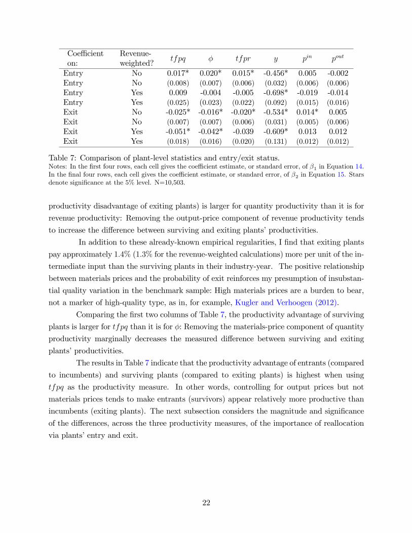
Table 7: Comparison of plant-level statistics and entry/exit status.Notes: In the first four rows, each cell gives the coeffi cient estimate, or standard error, of β1 in Equation 14.In the final four rows, each cell gives the coeffi cient estimate, or standard error, of β2 in Equation 15. Starsdenote significance at the 5% level. N=10,503.

productivity disadvantage of exiting plants) is larger for quantity productivity than it is for

revenue productivity: Removing the output-price component of revenue productivity tends

to increase the difference between surviving and exiting plants’productivities.

In addition to these already-known empirical regularities, I find that exiting plants

pay approximately 1.4% (1.3% for the revenue-weighted calculations) more per unit of the in-

termediate input than the surviving plants in their industry-year. The positive relationship

between materials prices and the probability of exit reinforces my presumption of insubstan-

tial quality variation in the benchmark sample: High materials prices are a burden to bear,

not a marker of high-quality type, as in, for example, Kugler and Verhoogen (2012).

Comparing the first two columns of Table 7, the productivity advantage of surviving

plants is larger for tfpq than it is for φ: Removing the materials-price component of quantity

productivity marginally decreases the measured difference between surviving and exiting

plants’productivities.

The results in Table 7 indicate that the productivity advantage of entrants (compared

to incumbents) and surviving plants (compared to exiting plants) is highest when using

tfpq as the productivity measure. In other words, controlling for output prices but not

materials prices tends to make entrants (survivors) appear relatively more productive than

incumbents (exiting plants). The next subsection considers the magnitude and significance

of the differences, across the three productivity measures, of the importance of reallocation

via plants’entry and exit.

22

3.5 Decompositions of Industry Productivity Growth

In this subsection, I compute the fraction of aggregate productivity growth that occurs

via the net entry effect: the exit of relatively unproductive plants and the entry of rela-

tively productive plants. The extent to which reallocation across plants explains aggregate

productivity growth has been extensively studied (e.g., Baily, Hulten, and Campbell 1992;

Griliches and Regev 1995; Foster, Haltiwanger, and Krizan 2001; and Foster, Haltiwanger,

and Syverson 2008). Of these analyses, I am most closely following Foster, Haltiwanger, and

Syverson (2008), who compute the net entry effect when either tfpr or tfpq is used as the

measure of plant productivity. Because entrants charge lower prices than incumbents, the

net entry effect is smaller when revenue productivity measures are used instead of quantity

productivity measures. The authors conclude that, "in terms of understanding the barriers

to allocative effi ciency... revenue based productivity decompositions may focus too much

attention on continuing businesses and not enough on the role of entering businesses." (p.

419) Below, I show that accounting for materials prices partially reverses this finding.

Like Foster, Haltiwanger, and Syverson (2008), I use the following growth decom-

position, due to Baily, Hulten, and Campbell (1992) and Foster, Haltiwanger, and Krizan

(2001):

∆tfpt =∑i∈C

θi,t−1 ·∆tfpit +∑i∈C

(tfpi,t−1 − tfpt−1

)·∆θit +

∑i∈C

∆tfpit ·∆θit (16)

+∑i∈N

θit · (tfpit − tfpt−1)︸ ︷︷ ︸Entry Effect

−∑i∈X

θi,t−1 · (tfpi,t−1 − tfpt−1)︸ ︷︷ ︸Exit Effect

In Equation 16, θit denotes the revenue share of plant i, within its industry, in year

t; tfpt gives the revenue-weighted average (log) productivity in year t; ∆ is the difference

operator; and C, N , and X are the sets of continuing, entering, and exiting plants. The

decomposition highlights the different sources of industry productivity growth, including the

Entry Effect, the Exit Effect, and the sum of the two effects (the Net Entry Effect).26 The

magnitudes of these three effects will depend on the productivity measure– either tfpr, tfpq,

or φ– used in Equation 16.

The results of the industry decompositions are given in Table 8. I decompose the

productivity growth– over 5-year intervals– separately for each of the 10 industries in the

benchmark sample. The values are the averages over these 10 industries. In the first four

26Since a large number of plants enter and exit my benchmark sample without actually entering or exitingtheir industries, I will be unable to distinguish among the sources of aggregate productivity growth that arelisted in the first line of Equation 16.

23

ProductivityMeasure

Total Entry ExitNetEntry

Total Entry ExitNetEntry

tfpr -1.60 -0.08 0.08 0.00 1.30 0.23 0.12 0.35tfpq -1.60 -0.06 0.15 0.09 1.30 0.32 0.12 0.44φ -1.60 -0.09 0.13 0.04 1.30 0.25* 0.14 0.39

Table 8: Aggregate productivity growth decompositions.Notes: All values are given as percentages, over five-year horizons. In the first four columns, industriesare assigned importance according to their total revenues. In the last four columns, industries are assignedimportance according to the number of plants. Stars indicate that the value given in the cell is significantlydifferent than the corresponding value that uses tfpq as the measure of plant productivity. See Web AppendixC for details.

columns, industries with larger revenues (primarily gasoline manufacturing) are given more

weight, while, in the last four columns, industries’weights are determined by the number

of plants in the industry. The main takeaway from the table is that the Net Entry term

is larger for quantity productivity (tfpq) than it is for either revenue productivity (tfpr) or

technical effi ciency (φ). Consistent with Foster, Haltiwanger, and Syverson (2008), Table 8

indicates that the contribution of net entry to aggregate productivity is larger when output

prices are accounted for. At the same time, accounting for materials prices reduces the

measured contribution of net entry to industry productivity growth. These patterns are

robust to the decomposition method and the relative weights given to different industries.27

For completeness’sake, I assess the statistical significance of the differences, across

the productivity measures, of the importance of the Entry, Exit, or Net Entry terms. When

industries are weighed by the number of plants, the Entry Effect is significantly greater

when φ– instead of tfpq– is used as the productivity measure. Other differences are not

statistically significant.

To summarize, the conventional productivity measures, tfpq and tfpr, reflect within-

industry differences in materials prices. Because exiting plants face relatively high materials

prices, and because (large) entrants pay relatively low prices, the difference between the

productivity of exiting and surviving plants (and between entrants and incumbents) is larger

for productivity measures that embody plants’materials prices. As a result, the contribution

27Foster, Haltiwanger, and Syverson (2008) consider a second growth decomposition, due to Griliches andRegev (1995). I show, in Web Appendix A.9, that this alternate decomposition method yields results verysimilar to those presented in Table 8.One problem with the productivity growth decompositions originates from the overrepresentation of large

plants in the benchmark sample. Because of this, entering and exiting plants are underrepresented inthe benchmark sample, and the decompositions understate the role of net entry as a source of aggregateproductivity growth. In Web Appendix A.10, I show that the qualitative patterns of this subsection (inparticular, the difference, in the size of the Net Entry Effect between the three productivity measures) holdafter correcting for the underrepresentation of entering and exiting plants.

24

of reallocation, via entry and exit, is smaller for the productivity measure, φ, that is cleansed

of materials prices. These differences, however, are small and only of marginal statistical

significance.

4 Sources of Materials Price Dispersion

I discuss three explanations for the observed within-industry dispersion of intermediate

input prices. The sources of materials price dispersion have implications for the social

benefits generated by each plant. Plants that pay low materials prices by taking advantage

of monopsonistic power are not providing any societal benefit: Low materials prices are a

transfer of profits from supplier to buyer. On the other hand, if plants pay low materials

prices because their suppliers are exceptionally productive, low materials prices represent

a positive impact on social welfare. The fraction of these welfare benefits that accrue to

consumers will depend, in turn, on the degree to which lower input prices are passed on to

final consumers.

To calculate the relative importance of these different sources of materials price dis-

persion, I need to impute, for each manufacturer, the identities of its suppliers. I outline, in

Section 4.1, the algorithm that I use to impute buyer-supplier relationships. In Section 4.2,

I compute the fraction of dispersion in tfpq and pin that can be explained by plants’geo-

graphic locations, their suppliers’marginal costs, and within-supplier deviations. A positive

correlation between plants’materials prices and their suppliers’marginal costs stimulates the

following question: If plants with low marginal cost suppliers pay less for their inputs, and if

having low materials prices is so advantageous, then what prevents plants from purchasing

their materials from the low marginal cost suppliers? In Section 4.3, I argue that buyer-

supplier relationships are persistent, suggesting that there is some inertial force that inhibits

all plants from switching to low marginal cost suppliers.28

4.1 Imputation of Buyer-Supplier Relationships

To impute buyer-supplier relationships, I use the algorithm introduced in Atalay, Hor-

taçsu, and Syverson (2013). The algorithm generates a list of establishments that could

potentially receive any shipment that is observed in the Commodity Flow Survey. Consider

a hypothetical shipment of commodity, c, made by establishment, h, to zip code, z. The

establishments, i, that could potentially receive this shipment are those who are located in

28Foster, Haltiwanger, and Syverson (2008) provide additional anecdotal evidence for the importance ofrelationship capital; see footnotes 23 and 24 of their paper.

25

z and are members of an industry that use c. For example, the potential recipients of a

shipment of Portland cement to z would be all plants in that zip code that are engaged

in road construction, concrete brick manufacturing, ready-mix concrete manufacturing, or

wholesaling of brick, stone, and related materials. If there are multiple potential recipients

of the shipment, and one of these establishments is owned by the same firm as the sending

establishment, then I assume that the shipment is received by the same-firm establishment.29

Otherwise, I assign each potential recipient, i, to be downstream of plant h.30

In order to compute suppliers’marginal costs, I require the upstream industry to

also be part of the manufacturing sector. Of the 10 industries in the benchmark sample,

only two– ready-mix concrete and corrugated boxes– have a main input that is produced

by a manufacturer. The industries with establishments that could potentially receive Port-

land cement (STCC=32411) are road construction firms (SIC=1610-1619), concrete brick

and block manufacturers (SIC=3271), ready-mix concrete manufacturers (SIC=3273), and

wholesalers of brick, stone, and related materials (SIC=5032).31,32 For paper and paperboard

manufacturers, I look for shipments in the Commodity Flow Survey for which the commodity

code is that of paperboard (STCC=26311 in 1993, SCTG=27319-27320 in 1997), which are

also sent to zip codes that contain establishments in either the corrugated and solid fiber

boxes (SIC=2653) industry or the folding paperboard boxes (SIC=2657) industry. Finally,

I drop shipments for which the unit price is greater than four times, or less than one-fourth,

the average for the industry-year.

For within-firm shipments, surveyed establishments do not report the actual market

value of the transaction. Instead, the establishments are asked to estimate what the value

of the shipment would have been had it been sold to some other firm. Since it is unclear

what these values actually represent, I remove downstream establishments who receive a

substantial fraction, 15% or more, of the relevant input from other plants from the same

29Atalay, Hortaçsu, and Syverson (2013) make the same assumption. This assumption is motivated bythe finding that establishment h is much more likely to ship to zip codes that contain an establishment fromthe same firm. The results of the current section are not sensitive to this assumption.30Assigning all potential recipients, i, to be downstream of plant h likely overcounts the number of buyer-

supplier relationships. In an unreported robustness check, I reproduce the analysis of Section 4.2, weighingobservations by the inverse of the number of potential recipients in the destination zip code. I find that theresults are essentially unchanged.31The commodity code used in the 1993 Commodity Flow Survey is the Standard Transportation Com-

modity Code (STCC). A list of STCC codes can be found in pages 117 to 167 of "Reference Guide forthe 2008 Surface Transportation Board Carload Waybill Sample," published by Railinc. Since 1997, theCommodity Flow Survey has used the Standard Classification of Transported Goods (SCTG) classificationof commodity codes. Documentation related to SCTG codes can be found on the Census web page.32Productivity data for cement and ready-mix concrete manufacturers are unavailable in 1997. So, for

cement and concrete manufacturers, I only look at buyer-supplier relationships in the 1993 Commodity FlowSurvey.

26

firm.33

4.2 Sources of Materials Price Dispersion

The purpose of this subsection is to describe and assess the quantitative importance of

the three potential sources of materials price variation.

I begin with some notation. Let χhit denote the total mass (in thousands of pounds)

of shipments sent by plant h to plant i in year t, and let ωhit denote the total value (in

thousands of real dollars) of shipments sent by plant h to plant i in year t. Then, the free

on board (f.o.b.)34 price that plant h charges plant i is simply the ratio of the value to the

price:

PCFShit ≡ ωhit

χhit(17)

The "CFS" superscript denotes prices computed using the Commodity Flow Survey data

(as opposed to the prices that are computed in Section 3, using data from the Census of

Manufacturers).35

For each downstream plant, i, input prices are defined by taking the value-weighted

average over all plants, h, that I observe i purchasing from:

P in,CFSit ≡

∑h∈Γ(i) ωhit · PCFS

hit∑h∈Γ(i) ωhit

(18)

In Equation 18, and throughout the remainder of this section, Γ(i) refers to the suppliers

of plant i, excluding the establishments that are in the same firm as plant i. Note that,

because it does not include freight charges, P in,CFSit will be less than what plants pay for

their intermediate inputs. I define a second plant-level input price, which includes freight

33While varying the 15% cutoff down to 0% or up to 25% does not affect this section’s results, therelationship between input prices and supplier productivity begins to disappear once the cutoff exceeds 25or 30%.Bernard, Jensen, and Schott (2006) show that reported prices on cross-border shipments, for which the

sender and receiver are part of the same firm, are manipulated to take advantage of the different tax policiesof the destination and source countries. Even though such an incentive to mis-report does not exist in theCommodity Flow Survey data, I argue that one should not put too much weight on input prices of the plantsthat buy a substantial fraction of their inputs from within the firm.34Unlike the (cost, insurance, and freight) c.i.f. price, the f.o.b. price does not include freight or insurance

charges.35The Commodity Flow Survey has, up to now, been an unexploited source of data on plants’ output

prices. With this in mind, I compare plants’output prices, derived from the Commodity Flow Survey to theprices derived from the better-known Census of Manufacturers. For the 66 cement manufacturers in thissection’s sample, the correlation between pout,CFSh and pouth is 39%. For the 162 paperboard manufacturers,the correlation between the two plant-level output prices is 60%.

27

charges:

P in,CFSit ≡

∑h∈Γ(i) ωhit ·

(PCFShit + τhit

)∑h∈Γ(i) ωhit

(19)

I estimate transportation costs, τhit, from the mileage of the shipment and the mode of

transport.36,37

Similar to the analysis of Section 3, all plant-level statistics are stated as the percent

deviation relative to the average value for the industry-year. Again, these deviations are

written using lower-case letters.

Geography

Geography is the first of the three sources of materials price variation. As discussed

in Section 3.3, of the 10 industries in the benchmark sample, concrete is the industry with

the strongest spatial correlation in materials prices, while the corrugated box industry dis-

plays relatively weak spatial correlation. Cement prices tend to be lower in areas with

an abundance of limestone, namely in the Appalachian and Great Lakes regions.38 To

assess the relationship between concrete plants’materials prices and their proximity to lime-

stone production, I regress– for the 3708 concrete plant-year observations in the benchmark

sample– pinijt against nearby employment in the limestone industry. The coeffi cient esti-

mates given in the final column of Table 9 imply that the materials price of concrete plants

is roughly 10% higher for plants that are in the 75th percentile of the limestone proximity

index, relative to plants in the 25th percentile.

Suppliers’Marginal Costs

Even within geographical areas, there is heterogeneity in plants’ suppliers’marginal

costs. For any concrete or corrugated box manufacturer, i, that is identified by the algorithm

36The Bureau of Transportation Statistics collects information on ton-mile freight charges for shipmentssent along different transport modes; see U.S. Department of Transportation (2009). Since the CommodityFlow Survey contains information on the weight of each shipment, as well as the distance that the shipmenttraveled, it is straightforward to estimate the shipment freight charge.37For the corrugated box manufacturing industry, I relate pin,CFSit and pinit . (Remember that p

init cannot

be computed in 1992 or 1997 for ready-mix concrete manufacturers.) The strength of this relationship,between the materials prices computed from the two data sources, indicates the success (or lack thereof) ofthe imputation procedure outlined in Section 4.1. The correlation between pin,CFSit and pinit is 22%, meaningthat I am mismeasuring many buyer-supplier relationships, but that the imputation algorithm yields a viabledataset.38In 1997, 48% of limestone shipment value originated from eight states– Alabama, Kentucky, Illinois,

Indiana, Ohio, Pennsylvania, Tennessee, and West Virginia– which represent roughly 24% of the U.S.population. See http://www.census.gov/prod/ec97/97n2123b.pdf for the state-by-state data on limestoneproduction.

28

Nearby limestone -0.043* -0.138* -0.232*employment (0.005) (0.012) (0.028)(Nearby limestone 0.047* 0.159*employment)2 (0.005) (0.028)(Nearby limestone -0.031*employment)3 (0.007)Adjusted R2 0.034 0.056 0.060

Table 9: Relationship between materials prices and nearby limestone production.Notes: Observations are revenue weighted. Stars indicate significance at the 5% level. N=3708.

outlined in Section 4.1, I compute average supplier productivity, TFPQit, as follows:

TFPQit ≡∑

h∈Γ(i) ωhit · TFPQht∑h∈Γ(i) ωhit

. (20)

The dispersion of tfpqit (the percent deviation of TFPQit from its industry-year

average) is substantial. For plants in the ready-mix-concrete (box-making) industry, the

standard deviation of tfpqit is 41% (26%). After including year by geographic division fixed

effects, the standard deviation of tfpqit is 36% for the ready-mix concrete industry, and 25%

for the corrugated box industry.39

Within-Supplier Price Differences

A third explanation for price variation lies in differences in the relative bargaining power

of the suppliers and buyers of any given material input, yielding variation in the prices that

suppliers charge, for the same good, across destinations. Define a supplier’s average output

price, P out,CFSht , as a value-weighted average of the prices that it charges in its Commodity

Flow Survey shipments. For each buyer-supplier relationship, I define the within-supplier

price deviation, ψhit, as:

ψhit ≡ log

(PCFShit

P out,CFSht

), (21)

where ψhit is the price that i pays for h’s output, relative to the other plants that buy

intermediate inputs from h; ψhit is positive provided plant i purchases its material inputs

from h at a higher price than P out,CFSht , the average output price of supplier, h.

Figure 1 decomposes the price distribution into two separate components. Any

buyer-supplier-specific price, pCFShit , is the sum of the supplier’s average output prices, pout,CFSht ,

and the within-supplier price deviation, ψhit. The price, pCFShit , that a supplier charges a buyer

39There are nine Census-defined divisions within the United States. Seehttp://www.census.gov/geo/www/us_regdiv.pdf for a correspondence between states and divisions.

29

02

46

Den

sity

­1 ­.5 0 .5 1Relativ e Price

Across Supplier Within Supplier Ov erall

Figure 1: Value-weighted price distributions.Notes: The sample includes all shipments sent by the cement and paperboard manufacturers that comprisedthe sample of the regression defined by Equation 23.

for intermediate inputs can be, mechanically, high for one of two reasons: either the supplier

has a high average price, pout,CFSht , or the supplier charges i a higher price than its other

customers (i.e., ψhit is large).40 For my sample of cement and paperboard manufactur-

ers, the distributions of pCFShit , ψhit, and pout,CFSht are depicted in Figure 1. The standard

deviation of pCFShit is 25%, larger than the standard deviation of suppliers’average output

prices (SD(pout,CFSht ) = 19%), and fifty percent larger than the standard deviation of the

within-supplier deviations (SD(ψhit) = 16%).41

The average within-supplier price deviation, ψit, measures the extent to which plant

i pays its supplier a higher materials price than the other customers of its suppliers. It is a

weighted average, over i’s suppliers, of the ψhit:

ψit ≡∑

h∈Γ(i) ωhit · ψhit∑h∈Γ(i) ωhit

=

∑h∈Γ(i) ωhit ·

(phit − pout,CFSht

)∑

h∈Γ(i) ωhit(22)

40Price discriminatory behavior, which would result from differences in buyers’and suppliers’bargainingpositions, is a first explanation for these within-supplier price differences. In addition, some of the within-supplier variation in materials prices may potentially be due to the time at which plant i receives its shipmentsfrom plant h. In Web Appendix A.11, I argue that, at least for this small sample of concrete and boxmanufacturers, the timing of shipments is not a primary source of materials price variation.41Figure 1 looks similar, whether one uses the sample of cement manufacturers, the sample of paperboard

manufacturers, or the pooled sample of paperboard and cement manufacturers. See Web Appendix A.12.

30

Sample Boxes Concrete Pooled

tfpqit-0.267*(0.059)

-0.257*(0.057)

-0.233*(0.056)

-0.201*(0.092)

-0.210(0.110)

-0.146(0.105)

-0.253*(0.050)

-0.243*(0.048)

-0.212*(0.047)

ψit0.340*(0.111)

0.691*(0.165)

0.406*(0.118)

N 190 190 190 131 131 131 321 321 321Adjusted R2 0.129 0.133 0.223 0.046 0.091 0.511 0.107 0.117 0.263Division F.E.? No Yes Yes No Yes Yes No Yes Yes

Table 10: Regression results.Notes: This table presents coeffi cient estimates and robust standard errors, from the regressions definedby Equation 23. The dependent variable in this regression is pin,CFSit . Observations are assigned weightsaccording to the revenues of plant i. Stars indicate significance at the 5% level.

Regression Results

Using these definitions, I can now compare the price that a plant pays for its mater-

ial inputs to differences in geography (summarized by division fixed effects), differences in

suppliers’marginal costs, and within-supplier price differences.42

pin,CFSit = βdivision + β1 · tfpqit + β2 · ψit + εit (23)

The results are presented in Table 10. A 10% increase in the marginal cost of

plants’suppliers corresponds to a 2.0% to 2.5% increase in plants’materials prices. The

estimated effect of supplier productivity on materials prices is somewhat stronger for boxes

than it is for ready-mix concrete. Including fixed effects for the geographic region of the

downstream plant has almost no effect on the estimate of β1.43 Finally, the coeffi cient

estimate, β 2, on the average within-supplier deviation term is positive and significant. Note

that, a mechanical relationship between ψit and pin,CFSit exists, as higher-than-average-priced

shipments will generate a large value for pin,CFSit (see Equation 19) and a large value of

ψit (see Equation 22). Measurement error in PCFShit , for example, will skew the coeffi cient

estimate of β2 towards 1.

Each cell in Table 11 presents the unexplained variation– measured as the (revenue-

weighted) standard deviation of the residuals– when pin,CFSit is regressed on different com-

binations of the right-hand side variables of Equation 23. Comparing the first and second

columns of Table 11, I calculate that the inclusion of division fixed effects reduces the un-

explained variation of materials prices by approximately 2%. The inclusion of suppliers’

42Using pin,CFSit instead of pin,CFSit as the dependent variable of the regression corresponding to Equation23 generates a similar estimate of β1.43It is possible that division fixed effects are too coarse to suffi ciently control for the geographic variation

in materials prices. Web Appendix A.13 presents evidence that this is not the case.

31

Include DivisionFixed Effects ?

No Yes No Yes No Yes No Yes

Include tfpqit ? No No Yes Yes No No Yes YesInclude ψit ? No No No No Yes Yes Yes Yes

Sample Sample SizeBoxes 190 0.187 0.180 0.174* 0.170* 0.175* 0.169* 0.164* 0.160*Concrete 131 0.359 0.338 0.349 0.330 0.268* 0.247* 0.262* 0.241*Pooled 321 0.209 0.204 0.197* 0.194* 0.189* 0.185* 0.180* 0.177*

Table 11: Unexplained materials price variation.Notes: Each cell gives the real-revenue-weighted standard deviation of the residuals in a particular regression;the full specification is given in Equation 23. Across the columns of the table, different combinationsof independent variables are included in the regressions. Stars indicate that the decline in dispersion issignificantly more than the decline that would occur from simply including "fake" random variables on theright-hand side of Equation 23. See Web Appendix C for details.

productivities reduces the unexplained variation by approximately 6%, while the two sets of

variables jointly reduce the unexplained price variation by 7%. Finally, the full combination

of right-hand-side variables– including the average within-supplier deviation– reduces the

unexplained variation of pin,CFSit by 15%. To summarize, both within-supplier and between-

supplier explanatory factors are significant and quantitatively important when accounting for

the dispersion in downstream plants’materials prices.44 These findings indicate that while

purely geographical considerations– such as spatial differences in resource abundance– drive

some of the differences in materials prices, the factor market’s competitive environment is

also of primary significance.

4.3 Persistence of Relationships

Buyer-supplier relationships are persistent across time, suggesting that there is some

force that inhibits intermediate inputs purchasers from switching suppliers. Whether this

inhibiting force reflects some extra profitability that is conferred by repeated interaction, or

some idiosyncratic match-specific productivity, it prevents all buyers from switching to the

lowest-cost intermediate goods suppliers.

To provide some empirical evidence for the persistence of buyer-supplier relation-

ships, I explore the shipments sent by cement and paperboard manufacturers in the 1993

and 1997 Commodity Flow Surveys. As before, the Commodity Flow Survey does not iden-

44Regarding the statistical significance of the results, note that any set of variables– for example, a randomvariable drawn from a standard normal distribution, or a set of 12 dummy variables that sum up to 1–will necessarily explain some positive fraction of the variation in pin,CFSi . In Web Appendix C, I testwhether the decline in dispersion is significantly greater than what would be expected from including differentcombinations of "fake" random variables on the right-hand side of Equation 23.

32

Sample Cement Cement Cement Paperboard Paperboard PaperboardLog Mileage -2.835 -2.594 -2.593 -1.025 -0.867 -0.881

(0.050) (0.050) (0.051) (0.024) 0.026 (0.026)Did the plant sell to 2.075 2.009 2.988 2.661the zip code in 1993? (0.105) (0.105) (0.067) (0.069)N 106,795 106,795 106,795 75,360 75,360 75,360Number of zip codes 2015 2015 2015 1256 1256 1256Number of plants 53 53 53 60 60 60Pseudo- R2 0.687 0.713 0.718 0.148 0.257 0.290Unconditional probabilityof shipping to zip code z

0.021 0.021 0.021 0.030 0.030 0.030

Include control forfirm presence in z?

No No Yes No No Yes

Table 12: Persistence of buyer-supplier relationships.Notes: This table presents coeffi cient estimates and standard errors, from the regression defined by Equation24. The sample is comprised of cement and paperboard plants that were included in the sample of Regression23. For a zip code to be in the sample, at least one plant in the sample must have shipped to the zip codein 1997.45

tify the downstream buyer. Instead, I proxy for the identity of the downstream buyer using

the destination zip code. I run a conditional logit regression, described by Equation 24; the

dependent variable equals 1 if the cement/paperboard plant, i, ships to zip code, z, in 1997.

The explanatory variable of interest is an indicator, which equals 1 if the plant shipped to

the zip code in 1993. Destination zip code-level fixed effects, supplier fixed effects, and the

log distance between i and z are additional explanatory variables.

I {i→ z in 1997} = βz + βi + β3 · log (distance i→ z) + β4 · I {i→ z in 1993} (24)

+ β5 · I {plant of i’s firm is located in z in 1997}+ εiz

The results are presented in Table 12. Both cement and paperboard suppliers’

decisions on which destinations to ship to are persistent across time. If plant i sells to zip

code z in 1993, the probability that i will sell to z in 1997 is much larger, approximately

6 to 8 times larger for cement manufacturers, and 10 to 14 times larger for paperboard

manufacturers.45In addition, I restrict the sample to establishments that were sampled in both the 1993 and 1997

Commodity Flow Surveys. Secondly, in order to comply with Census disclosure rules, I restrict the sampleto plants that are members of firms, f , such that the following three criteria hold: a) there exists at leastone i, z pair for which plant i (owned by f) shipped to z in 1993, but not in 1997; b) there exists at leastone i, z pair for which plant i shipped to z in 1997, but not in 1993; and c) there exists at least one i, zpair for which i shipped to z in both 1993 and 1997. The coeffi cient estimates are similar when the sampleis constructed without this second restriction.

33

There are two distinct interpretations of the positive estimate on, β4, the coeffi cient

on the persistence of buyer-supplier relationships (see, for example, Dubé, Hitsch, and Rossi

2010). In the first interpretation, an establishment’s profitability of working with a counter-

party increases from having transacted with that counterparty in the past. Kellogg (2011),

for instance, documents that oil production companies and drillers become more productive

as they gain experience working with one another. According to the second interpretation,

some establishments happen to find it more profitable to work with certain counterparties

for idiosyncratic reasons, other than geographic proximity. The estimate of the persistence

term, β4, will be positive provided these idiosyncratic factors display some persistence. Un-

fortunately, the data that I have at hand do not permit me to distinguish between these

two interpretations. Either interpretation, however, is consistent with downstream estab-

lishments that decide to remain matched with high marginal cost suppliers.

5 Conclusion

In this paper, I have studied the consequences and sources of materials price dispersion.

Variation in materials prices explains a substantial fraction of the variation in plants’mar-

ginal costs, revenue total factor productivities, and probabilities of survival. Moreover, one

reason why some plants have low materials prices is that they have access to suppliers with

low marginal costs.

The paper’s results suggest that establishments’survival and growth prospects are

directly related to those of their customers and/or suppliers. In future work, I hope to

investigate the relationship between establishments’growth and the growth rates of their

counterparties. Such an investigation will be an important building block in understanding

the propensity with which shocks to a small set of firms have the potential to cascade

throughout the economy and produce aggregate fluctuations.

A Robustness Checks and Other Calculations

A.1 Industries with Heterogeneous Quality Outputs

In this subsection, I reproduce the empirical analysis of Sections 3.1, 3.2, and 3.3 for

a set of industries that display substantial output quality variation. The four industries

that I choose for this exercise are cucumber pickles, sausages, softwood cut stock, and wine.

Details on the construction of the sample can be found in Web Appendix B.2.

Correlations among plant-level characteristics are presented in Table 13. Compared

34

pin pout tfpq φ tfprpout 0.284*tfpq -0.273* -0.808*φ 0.254* -0.659* 0.858*tfpr 0.024 0.329* 0.305* 0.290*Std. Dev. 0.318 0.385 0.380 0.380 0.237

Table 13: Correlations and standard deviations of plant-level characteristics.Notes: Observations are revenue weighted. Stars indicate that the correlation is significantly different from0, at the 5% level (see Web Appendix C for details). N=1256.

Dispersion of tfpq Dispersion of φ Percent DeclineSample 90/10 75/25 SD 90/10 75/25 SD 90/10 75/25 SD NPickles 0.891 0.446 0.344 0.881 0.412 0.339 1.2% 8.6% 1.3% 145Sausages 0.727 0.399 0.295 0.747 0.366 0.301 -2.7% 9.5% -2.0% 621Softwood 1.571 0.818 0.547 1.316 0.697 0.477 21.4%* 18.9% 16.0%* 160Wine 1.314 0.696 0.479 1.268 0.726 0.481 3.6% -4.0% -0.5% 330Pooled 0.948 0.494 0.380 0.977 0.486 0.380 -2.9% 1.7% 0.0% 1256

Table 14: Dispersion of tfpq and φ.Notes: Observations are revenue weighted. Stars indicate that the difference between tfpq and φ is statisti-cally significant, at the 5% level (see Web Appendix C for details).

to the benchmark sample, the standard deviations of most plant-level characteristics are

larger, while the correlations among the different productivity measures are, in general,

weaker. While the correlation between tfpr and pin is negative (−0.232) and significant in

the benchmark sample, in the Quality Variation sample there is essentially no relationship

between input prices and revenue productivity. Within the Quality Variation sample, high

materials prices reflect high-quality inputs, which in turn lead to greater profitability. (There

is still the countervailing relationship– as for the benchmark sample– where high materials

prices reflect unfavorable factor market conditions, potentially lowering profitability.)

The dispersions of tfpq and φ are given in Table 14. For the pooled sample,

the dispersions of the two distributions are essentially the same. Looking across the four

industries, there is a significant decline in productivity dispersion for one of the industries,

softwood cut stock, and no difference for the other three industries.

In Table 15, I present regression results, in which I regress plants’materials prices

against the materials prices of nearby plants (those within 250 miles, in the same industry-

year). The fraction of materials price variation that is explained by neighbors’ average

materials prices is essentially 0 for each of the four industries in the Quality Variation sample.

In summation, output quality variation has the potential to severely attenuate the

difference between the dispersions of φ and tfpq. To the extent that any quality variation

35

Sample β s.e. Adjusted R2

Pickles 0.124 0.130 -0.001Sausages 0.038 0.075 -0.001Softwood -0.165 0.137 0.003Wine -0.456 0.195 0.013Pooled -0.017 0.064 -0.001

Table 15: Spatial correlation of materials prices.Notes: The dependent variable is pinijt, and the independent variable is the (revenue-weighted) average of thepini′jt for the plants that are within a 250-mile radius of plant i in industry j and year t. Observations arerevenue weighted.

exists in the benchmark sample, the difference between the dispersions of φ and tfpq, as

reported in Table 3, may be downwardly biased.

A.2 Variation in Input Quality

One of the main presumptions of the empirical analysis is that variation in input quality

is not an important source of variation of input prices. I have chosen industries to try to

minimize the role of input quality differentiation. There is one specific industry, ready-

mix concrete, for which there is reason to suspect that input quality differences could be

contaminating some of the results. In this subsection, I explain why input quality varies

across plants, and then determine how big of an effect input quality variation has on the

observed relationships between input prices and different productivity measures.

Portland cement, the main intermediate input used in the production of ready-mix

concrete, comes in four types, labeled type I, II, III, or IV.46 Type-I and II cement account

for over 90% of the expenditures on cement, with the majority of sales coming from type-

I cement (U.S. Department of Interior 1989). In areas where the soil has high sulfate

concentrations, type-II cement may be preferable to the less expensive type-I cement, since

ready-mix concrete produced using type-I cement is susceptible to sulfate attack (cracking

or loss of strength in the presence of sulfate). Since high sulfate concentrations exist only

in the soil of parts of the western third of the United States, one should observe type-I and

type-II cement consumed in the western United States, and only type-I cement consumed in

the remainder of the United States.47

46The standards for the different types of Portland cement are set by the American Society for Testingand Materials (ASTM). See the ASTM web page for more information on the distinguishing features ofdifferent types of Portland cement: http://www.astm.org/Standards/C150.htm .47Cement type is not recorded in the Census of Manufacturers materials file. I confirm, using the Census

of Manufacturers production file, that only type-I cement is produced by plants in the eastern two-thirds ofthe United States, while both types I and II are produced in the western U.S.

36

Sample pin, tfpq pin, φ pin, pout pin, tfpr φ, tfpq tfpq, tfpr tfpq, pout NEntire U.S. -0.306* 0.120* 0.276* -0.127* 0.908* 0.741* -0.476* 3708Divisions 1-7 -0.341* 0.089* 0.251* -0.180* 0.906* 0.750* -0.430* 3049Divisions 8-9 -0.351* 0.066 0.360* -0.105 0.911* 0.688* -0.597* 659

Table 16: Correlations among plant-level characteristics.Notes: Observations are revenue weighted. Stars indicate that the correlation is significantly different from0, at the 5% level.

Dispersion of tfpq Dispersion of φ Percent DeclineSample 90/10 75/25 SD 90/10 75/25 SD 90/10 75/25 SD N

Entire U.S. 0.521 0.251 0.224 0.486 0.236 0.215 7.4%* 6.6%* 4.4%* 3708Divisions 1-7 0.486 0.238 0.211 0.439 0.222 0.199 11.3%* 7.7%* 6.2%* 3049Divisions 8-9 0.611 0.296 0.255 0.570 0.253 0.239 7.4% 18.3%* 6.9%* 659

Table 17: Dispersion of tfpq and φ.Notes: Stars indicate that the difference between tfpq and φ is statistically significant, at the 5% level.

Given this geographic difference in soil composition, I split the sample of ready-mix

concrete plants into two subsamples: plants residing in Census divisions 1-7, and plants lo-

cated in Census divisions 8-9.48 The dispersion of pin is larger in divisions 8-9 (20.0%, versus

17.0% for divisions 1-7), as some ready-mix concrete plants purchase the low price type-I ce-

ment, while others must purchase the high price type-II cement. In contrast, in the eastern

United States, virtually all ready-mix concrete plants purchase type-I cement, leading to a

more compressed pin distribution. For both subsamples, tfpq and pin are inversely related

to one another, with the negative relationship between tfpq and pin somewhat stronger in

the eastern United States; see Table 16. These geographic differences are consistent with

greater cement quality variation in the western United States.

In Table 17, I compute the dispersion of tfpq and φ for the ready-mix concrete

subsamples. The decline in dispersion is larger for each of the two subsamples than it is for

the pooled sample of 3708 ready-mix concrete plants.

In Table 18, I assess the spatial correlation of materials prices, separately for plants

in the eastern and western United States. Materials prices are strongly spatially correlated,

within each of the two parts of the U.S. Thus, it does not seem as if the spatial correlation

of cement prices is primarily due to higher-than-average input quality in the western U.S.

In summation, there is almost no variation in the quality of cement purchased by

ready-mix concrete plants in the eastern two-thirds of the United States. For this subsample,

the difference between the standard deviation of tfpq and the standard deviation of φ is 2 to

48Census division 8 is made up of Arizona, Colorado, Idaho, Montana, Nevada, New Mexico, Utah, andWyoming, while Census division 9 includes Alaska, California, Hawaii, Oregon, and Washington.

37

Sample β s.e. Adjusted R2

Entire U.S. 0.913 0.028 0.222Divisions 1-7 0.936 0.033 0.210Divisions 8-9 0.812 0.068 0.177

Table 18: Spatial correlation of materials prices.Notes: The dependent variable is pinijt, and the independent variable is the (revenue-weighted) average of thepini′jt for the plants that are within a 250-mile radius of plant i in industry j and year t. Observations arerevenue weighted.

3 percentage points larger than the differences that are reported in Table 3. So, a moderate

amount of materials quality variation would probably cause me to somewhat underreport

the fraction of productivity dispersion that is due to differences in factor market conditions.

References

Ackerberg, Daniel A., Kevin Caves, and Garth Frazer (2006). "Structural Identification of

Production Functions." Working paper, University of Toronto.

Atalay, Enghin, Ali Hortaçsu, and Chad Syverson (2013). "Vertical Integration and Input

Flows." Working paper, University of Chicago.

Baily, N. Martin, Charles R. Hulten, and David Campbell (1992). "Productivity Dynamics

in Manufacturing Plants." Brookings Papers on Economic Activity: Microeconomics,

1992, 187-249.

Balasubramanian, Natarajan and Jagadeesh Sivadasan (2011). "What Happens When

Firms Patent? New Evidence from U.S. Economic Census Data." Review of Economics

and Statistics, 93, 126—146.

Bernard, Andrew B. and J. Bradford Jensen (1999). "Exceptional Exporter Performance:

Cause, Effect, or Both?" Journal of International Economics, 47, 1—25.

Bernard, Andrew B., J. Bradford Jensen, and Peter Schott (2006). "Transfer Pricing by

U.S.-Based Multinational Firms." NBER Working Paper No. 12493.

Bloom, Nicholas and John Van Reenen (2010). "Why Do Management Practices Differ

Across Firms and Countries?" Journal of Economic Perspectives, 24, 203—224.

Blundell, Richard and Stephen Bond (2000). "GMMEstimation with Persistent Panel Data:

An Application to Production Functions." Econometric Reviews, 19, 321-340.

Caves Douglas, Laurits Christensen, and Erwin Diewert (1982). "Multilateral Compar-

isons of Output, Input, and Productivity Using Superlative Index Numbers." Economic

38

Journal, 92, 73-86.

Collard-Wexler, Allan and Jan De Loecker (2013). "Reallocation and Technology: Evidence

from the U.S. Steel Industry." NBER Working Paper No. 18739.

Davis, Steven, Cheryl Grim, and John Haltiwanger (2008). "Productivity Dispersion and

Input Prices: The Case of Electricity." CES Working Paper Series No. 08-33.

Dubé, Jean-Pierre, Günter J. Hitsch, and Peter E. Rossi (2010). "State Dependence and

Alternative Explanations for Consumer Inertia." RAND Journal of Economics, 41, 417-

445.

Eslava, Marcela, John Haltiwanger, Adriana Kugler, and Maurice Kugler (2004). "The

Effects of Structural Reforms on Productivity and Profitability Enhancing Reallocation:

Evidence from Colombia." Journal of Development Economics, 75, 333-371.

Eslava, Marcela, John Haltiwanger, Adriana Kugler, and Maurice Kugler (2013). "Trade

Reforms and Market Selection: Evidence from Manufacturing Plants in Colombia."

Review of Economic Dynamics, 16, 135-158.

Foster, Lucia, John Haltiwanger, and C. J. Krizan (2001). "Aggregate Productivity Growth:

Lessons from Microeconomic Evidence." In New Developments in Productivity Analy-

sis, edited by Charles R. Hulten, Edwin R. Dean, and Michael J. Harper. Chicago:

University of Chicago Press, 303-372.

Foster, Lucia, John Haltiwanger, and Chad Syverson (2008). "Reallocation, Firm Turnover,

and Effi ciency: Selection on Productivity or Profitability?" American Economic Review,

98, 394—425.

Fox, Jeremy and Valérie Smeets (2011). "Does Input Quality Drive Measured Differences

in Firm Productivity?" International Economic Review, 52, 961-989.

Gandhi, Amit, Salvador Navarro, and David Rivers (2012). "On the Identification of Pro-

duction Functions: How Heterogeneous is Productivity?" Working paper, University of

Wisconsin, Madison.

Gorodnichenko, Yuriy (2010). "Using Firm Optimization to Evaluate and Estimate Pro-

ductivity and Returns to Scale." Working paper, University of California, Berkeley.

Griliches, Zvi and Haim Regev (1995). "Firm Productivity in Israeli Industry: 1979-1988."

Journal of Econometrics, 65, 175-203.

Hsieh, Chang-Tai and Peter J. Klenow (2009). "Misallocation and Manufacturing TFP in

China and India." Quarterly Journal of Economics, 124, 1403—1448.

Katayama, Hajime, Shihua Lu, and James R. Tybout (2009). "Firm-Level Productivity

Studies: Illusions and a Solution." International Journal of Industrial Organization, 27,

403-413.

Kellogg, Ryan (2011). "Learning by Drilling: Inter-Firm Learning and Relationship Persis-

39

tence in the Texas Oilpatch." Quarterly Journal of Economics, 126, 1961-2004.

Klump, Rainer, Peter McAdam, and Alpo William (2012). "The Normalized CES Produc-

tion Function: Theory and Empirics." Journal of Economic Surveys, 26, 769-799.

Kugler, Maurice and Eric Verhoogen (2012). "Prices, Plant Size, and Product Quality."

Review of Economic Studies, 79, 307-339.

Manova, Kalina and Zhiwei Zhang (2012). "Export Prices Across Firms and Destinations."

Quarterly Journal of Economics, 127, 379-436.

Olley, G. Steven and Ariel Pakes (1996). "The Dynamics of Productivity in the Telecom-

munications Equipment Industry." Econometrica, 64, 1263—1297.

Ornaghi, Carmine (2006). "Assessing the Effects of Measurement Errors on the Estimation

of Production Functions." Journal of Applied Econometrics, 21, 879—891.

Raval, Devesh (2011). "Non Neutral Technology and the Microeconomic Production Func-

tion." CES Working Paper Series No. 11-05.

Roberts, Mark J. and Dylan Supina (1996). "Output Price, Markups, and Producer Size."

European Economic Review, 40, 909-921.

Roberts, Mark J. and Dylan Supina (2000). "Output Price and Markup Dispersion in

Micro Data: The Roles of Producer Heterogeneity and Noise." In Advances in Applied

Microeconomics, Vol. 9, Industrial Organization, edited by Michael R. Baye. Greenwich:

JAI Press, 1—36.

Syverson, Chad (2004a). "Product Substitutability and Productivity Dispersion." Review

of Economics and Statistics, 86, 534—550.

Syverson, Chad (2004b). "Market Structure and Productivity: A Concrete Example."

Journal of Political Economy, 112, 1181—1222.

U.S. Department of the Interior (1989). Cement Mineral Yearbook.

U.S. Department of Transportation, Bureau of Transportation Statistics (2009). Table 3-21:

Average Freight Revenue Per Ton-mile.

van Biesebroeck, Johannes (2008). "The Sensitivity of Productivity Estimates: Revisiting

Three Important Debates." Journal of Business and Economic Statistics, 26, 311-328.

40

A.3 Substitution Between Material Inputs and Other Inputs

The empirical analysis of Section 3 invokes the assumption that the elasticity of sub-

stitution, %, between material inputs and all other inputs equals 1 (see Assumption 1). In

reality, material inputs are likely to be complements to other inputs. In this subsection, I

analyze how the dispersion of φ differs under different assumptions on %.

Consider a plant with technical effi ciency Φijt. Assume that, for plant i, the price of

a unit of the "priced" intermediate input is P inijt, and let the corresponding industry-year

average be P injt . The prices of the other inputs are assumed to be the same for all plants

in the industry-year (see Assumption 2). With an elasticity of substitution of %, plant i’s

marginal cost equals:

MCijt =1

Φijt

Sjt · σjt ·(P inijt

P injt

)1−%

+ 1− Sjt · σjt

11−%

(25)

As in Section 3, σjt ·Sjt refers to the expenditure share of "priced" materials. Equation25 states that plants’marginal costs are determined by their technical effi ciencies (Φijt) and

the composite price that they face for intermediate inputs and other inputs. The elasticity,

%, dictates how the prices of intermediate inputs and other inputs are combined. As %

decreases, a larger weight is allotted to the input with a higher relative price.

Re-arranging Equation 25 yields the following expression for Φijt in terms of TFPQijt

and P inijt:

Φijt = TFPQijt

Sjt · σjt ·(P inijt

P injt

)1−%

+ 1− Sjt · σjt

11−%

(26)

For the pooled benchmark sample, I use Equation 26 to compute the standard deviation

of φijt, for % ∈ {0.2, 0.4, .0.6, 0.8, 1.0}. These results, which are presented in Table 19,

illustrate that the dispersion of φ is robust to changes in the elasticity of substitution, even

as % approaches 0. Varying the elasticity of substitution, %, only has a noticeable effect

on the measured technical effi ciency for plants that have very small or very large values of

P inijt ÷ P in

jt . Since most plants have materials prices that are close to the industry average,

% does not substantially alter the measured dispersion of φ.

A.4 Substitution Across Material Inputs

Throughout the body of the paper, I assume that the elasticity of substitution between

different material inputs– for industries that use multiple material inputs– is 0 (see As-

A-1

% 0.2 0.4 0.6 0.8 1.0Revenue- Yes 0.1507 0.1507 0.1507 0.1507 0.1506weighted? No 0.2193 0.2192 0.2192 0.2191 0.2191

Table 19: Dispersion of φ, as computed using Equations 9 and 26.Notes: The dispersion of φ, when % = 1.0, equals the value given in the final row of Table 3. N=10,503.

SampleRevenue-weighted?

90/10 SD 90/10 SD 90/10 SD N

% 0.1 0.1 0.3 0.3 0.5 0.5Concrete No 0.5223 0.2302 0.5223 0.2302 0.5222 0.2303 3708

Yes 0.4864 0.2151 0.4863 0.2151 0.4862 0.2151 3708Pooled No 0.4930 0.2190 0.4929 0.2190 0.4928 0.2191 10,503

Yes 0.3240 0.1506 0.3240 0.1506 0.3240 0.1506 10,503

Table 20: Dispersion of φ, as computed using Equations 8, 9, and 27.

sumption 4). For plants that produce ready-mix concrete, I assess the importance of the

assumption that plants may not substitute across different material inputs.

When the elasticity of substitution between gravel/sand and cement is constant (but

not necessarily 0), the price of a bundle of material inputs equals:

P inijt ≡

sGraveljt

sGraveljt + sCementjt

·(P inGravel,ijt

P inGravel,jt

)1−%

+sCementjt

sGraveljt + sCementjt

·(P inCement,ijt

P inCement,jt

)1−% 1

1−%

(27)

In Equation 27, sGraveljt refers to the share of materials expenditures that go to gravel,

P inGravel,ijt is the price that plant i pays per 1000 pounds of gravel in year t, P

inGravel,ijt is the

geometric average of the price paid by all ready-mix concrete producing plants in year t, and

% is the elasticity of substitution between cement and sand/gravel. In the baseline analysis,

I had set % = 0.

Using Equation 27, I compute ready-mix concrete plants’materials prices. I then re-

compute Φijt, using Equation 8, and φijt, using Equation 9. The dispersion of φ is given in

Table 20. As % increases, the price of a bundle of intermediate inputs decreases for plants

that have exceptionally cheap input prices for one of the two intermediate inputs. Also, as

% increases, the relative price of the bundle increases for plants that pay roughly the same

relative price for the two intermediate inputs. It turns out that, in combination, these two

effects have almost no impact on the overall dispersion of φ.

A-2

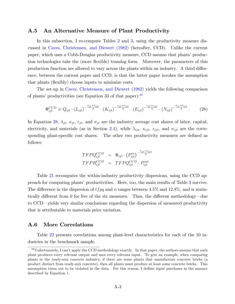
A.5 An Alternative Measure of Plant Productivity

In this subsection, I re-compute Tables 2 and 3, using the productivity measure dis-

cussed in Caves, Christensen, and Diewert (1982) (hereafter, CCD). Unlike the current

paper, which uses a Cobb-Douglas productivity measure, CCD assume that plants’produc-

tion technologies take the (more flexible) translog form. Moreover, the parameters of this

production function are allowed to vary across the plants within an industry. A third differ-

ence, between the current paper and CCD, is that the latter paper invokes the assumption

that plants (flexibly) choose inputs to minimize costs.

The set-up in Caves, Christensen, and Diewert (1982) yields the following comparison

of plants’productivities (see Equation 33 of that paper):49

ΦCCDijt ≡ Qijt · (Lijt)−

λjt+λijt2 · (Kijt)

−κjt+κijt2 · (Eijt)−

εjt+εijt2 · (Nijt)

−σjt+σijt2 . (28)

In Equation 28, λjt, κjt, εjt, and σjt are the industry average cost shares of labor, capital,

electricity, and materials (as in Section 2.4), while λijt, κijt, εijt, and σijt are the corre-

sponding plant-specific cost shares. The other two productivity measures are defined as

follows:

TFPQCCDijt = Φijt ·

(P inijt

)−σjt+σijt2

TFPRCCDijt = TFPQCCD

ijt · P outijt

Table 21 recomputes the within-industry productivity dispersions, using the CCD ap-

proach for computing plants’productivities. Here, too, the main results of Table 3 survive.

The difference in the dispersion of tfpq and φ ranges between 4.5% and 12.8%, and is statis-

tically different from 0 for five of the six measures. Thus, the different methodology– due

to CCD– yields very similar conclusions regarding the dispersion of measured productivity

that is attributable to materials price variation.

A.6 More Correlations

Table 22 presents correlations among plant-level characteristics for each of the 10 in-

dustries in the benchmark sample.

49Unfortunately, I can’t apply the CCD methodology exactly. In that paper, the authors assume that eachplant produces every relevant output and uses every relevant input. To give an example, when comparingplants in the ready-mix concrete industry, if there are some plants that manufacture concrete bricks (aproduct distinct from ready-mix concrete), then all plants must produce at least some concrete bricks. Thisassumption turns out to be violated in the data. For this reason, I deflate input purchases in the mannerdescribed by Equation 1.

A-3

Revenue- Dispersion of tfpqCCD Dispersion of φCCD Percent Declineweighted? 90/10 75/25 SD 90/10 75/25 SD 90/10 75/25 SDYes 0.438 0.203 0.193 0.391 0.193 0.177 12.8%* 5.7% 6.4%*No 0.521 0.249 0.234 0.489 0.234 0.219 6.7%* 6.5%* 4.5%*

Table 21: Dispersion of tfpq and φ.Notes: In the final three columns, stars indicate that the difference between tfpq and φ is statisticallysignificant, at the 5% level (see Web Appendix C for details).

Sample pin, tfpq pin, φ pin, pout pin, tfpr φ, tfpq tfpq, tfpr tfpq, pout

Boxes, Yr.≤’87 -0.286* 0.226* 0.280* -0.042 0.868* 0.418* -0.797*Boxes, Yr.≥’92 -0.352* 0.089 0.286* -0.086* 0.901* 0.116* -0.877*Coffee -0.485* 0.030 0.343* -0.227 0.855* 0.592* -0.584*Concrete -0.306* 0.120* 0.276* -0.127* 0.908* 0.740* -0.476*Flour -0.394* 0.468* 0.312* -0.011 0.628* 0.128 -0.722*Gasoline -0.395* 0.141* 0.171* -0.310* 0.854* 0.824* -0.368*Milk, Bulk -0.424* -0.149 0.410* -0.072 0.958* 0.444* -0.770*Milk, Packaged -0.281* 0.049 0.225* -0.104* 0.945* 0.435* -0.754*Sugar -0.034 0.481* 0.237* 0.100 0.860* 0.858* -0.466*Yarn -0.301* 0.197 0.211* -0.174* 0.875* 0.491* -0.763*Pooled -0.369* 0.127* 0.231* -0.232* 0.873* 0.694* -0.551*

Table 22: Correlations among plant-level characteristics.Notes: Stars indicate that the correlation is significantly different from 0, at the 5% level (see Web AppendixC for details).

For several of the correlations, the subsample of raw cane sugar manufacturing plants is

anomalous. For this industry, plants’marginal costs are unrelated to their materials prices.

Moreover, the correlation between input prices and technical effi ciencies is much stronger

(48%) than for other subsamples. These patterns are somewhat puzzling. Most likely,

either there is substantial measurement error in the physical units that cane sugar refiners

use, or there is significant quality heterogeneity among the raw cane sugar manufacturers.

Except for the raw cane sugar industry, correlations among plant-level characteristics are

qualitatively similar across the different industries in the benchmark sample. The correlation

between materials prices and quantity productivities is moderately negative for the nine other

industries, while the correlation between quantity productivities and output prices is strongly

negative (ranging between −37% and −88%). Finally, the three productivity measures are

always highly correlated with one another, with the correlation between φ and tfpq being

larger than the correlation between tfpq and tfpr.

A-4

A.7 Measurement Error

As discussed in Section 3.2, measurement error in the quantities that a plant consumes

or produces has the potential to bias the correlations among plant-level characteristics. In

this subsection, I assess the importance of measurement error.

To do so, I perform an exercise in which I add a randomly-generated disturbance to

plant-level input and output quantities, and then re-compute the plant-level productivity

measures. In particular, for each of the 10, 503 plant-year observations in the benchmark

sample, I take two draws from a standard normal distribution. Use υijt and $ijt to re-

fer to these randomly-generated numbers for plant i, in industry j, and year t. I apply

these randomly-generated numbers to the physical quantities of input and output purchases,

yielding "contaminated" physical quantity measures:

qijt = qijt + ϑ · υijt (29)

nijt = nijt + ϑ ·$ijt (30)

In Equation 29-30, and throughout the rest of this subsection, x will refer to the version

of any plant-level characteristic, x, that is imbued with extra measurement error. ϑ is a

parameter that characterizes the amount extra measurement error.

The definitions of plants’input prices, output prices, and productivity measures follow

from Equations 29-30, in combination with Equations 3-8:

poutijt = poutijt − ϑ · υijt (31)

pinijt = pinijt − ϑ ·$ijt (32)

tfpqijt = tfpqijt + ϑ · υijt (33)

φijt = φijt + ϑ · υijt − Sjt · σjt · ϑ ·$ijt (34)

In this exercise, no extra measurement error is applied to the revenue productivity measure

(tfpr), because both qijt and nijt are absent in the computation of this variable.

Correlations among the contaminated plant-level characteristics are presented in Table

23. Table 24 displays the standard deviations of φ, tfpq, pin, and pout, in addition to the

5-year autocorrelation coeffi cients of φ, tfpq, pin, and pout. The takeaways from Tables 23

and 24 are that measurement error in input and output quantities magnifies the correla-

tion between input prices and technical effi ciency, and between output prices and quantity

productivity. Second, measurement error attenuates the correlation between input prices

and quantity productivity, and between input prices and revenue productivity. Third, mea-

surement error increases the dispersions of quantity productivity and technical effi ciency,

A-5

ϑ pin, tfpq pin, φ pin, pout pin, tfpr φ, tfpq tfpq, tfpr tfpq, pout

0.01 -0.366 0.128 0.226 -0.234 0.874 0.694 -0.5530.02 -0.360 0.135 0.218 -0.234 0.874 0.691 -0.5580.03 -0.350 0.147 0.207 -0.232 0.873 0.687 -0.5680.04 -0.337 0.163 0.195 -0.229 0.872 0.680 -0.5800.05 -0.323 0.182 0.182 -0.225 0.870 0.671 -0.5950.06 -0.306 0.203 0.168 -0.220 0.868 0.660 -0.6120.07 -0.289 0.226 0.155 -0.215 0.865 0.648 -0.6310.08 -0.271 0.249 0.141 -0.208 0.863 0.635 -0.6500.09 -0.254 0.272 0.128 -0.202 0.860 0.621 -0.6690.10 -0.237 0.294 0.116 -0.195 0.857 0.607 -0.688

Table 23: Biases generated by measurement error.Notes: The table presents correlations among plant-level characteristics. In a given row, the standarddeviation of the extra measurement error is given by ϑ. In the calculations, observations are weighed by realrevenues.

with a larger increase in the dispersion of the technical effi ciency term. (Since the technical

effi ciency term is computed using both input and output quantities, it is the more sensitive

to measurement error.) Finally, measurement error reduces the estimated persistence of the

plant-level input prices, output prices, and productivity measures.

A.8 Unweighted Results

In this subsection, I present the unweighted versions of Tables 2, 3, 6, 14, 15, and 22.

In the benchmark calculations, observations are revenue weighted. To preview the main

results, all of the main conclusions of Section 3 are robust to the weighting scheme.

The first two tables, Tables 25 and 26, give the correlations among plant-level statis-

tics. Overall, the correlation between pin and pout is somewhat larger, while the correlation

between pin and tfpq is somewhat closer to 0, compared to the correlations contained in

Tables 2 and 22.

Compared to the revenue-weighted calculations, the unweighted dispersions of tfpr,

tfpq, and φ are larger (see the first eleven rows of Table 27 for the benchmark sample,

and the final five rows for the Quality Variation sample). The larger dispersions have

two sources. First, revenue weighting gives more importance to high revenue-per-plant

industries. Since gasoline, which by far has the largest average revenues among the industries

in the benchmark sample, has more compressed tfpr, tfpq, and φ distributions, assigning

weights by revenue causes the pooled dispersion to be larger in the unweighted calculations.

Second, the unweighted calculations give relatively more weight, within industries, to the

low productivity, low employment plants, again causing unweighted dispersions to be larger

A-6

Std. Dev. Persistence

ϑ tfpq φ pout pin tfpq φ pin pout

0.01 0.161 0.151 0.117 0.119 0.180 0.186 0.320 0.3050.02 0.162 0.152 0.117 0.120 0.184 0.185 0.308 0.3000.03 0.163 0.155 0.119 0.121 0.187 0.182 0.290 0.2920.04 0.165 0.158 0.121 0.124 0.189 0.177 0.268 0.2810.05 0.168 0.162 0.124 0.127 0.189 0.170 0.244 0.2680.06 0.171 0.166 0.128 0.131 0.189 0.163 0.217 0.2540.07 0.174 0.172 0.132 0.135 0.187 0.154 0.191 0.2390.08 0.178 0.177 0.136 0.140 0.185 0.146 0.165 0.2240.09 0.182 0.184 0.142 0.145 0.182 0.137 0.141 0.2100.10 0.187 0.191 0.147 0.151 0.178 0.128 0.118 0.197

Table 24: Biases generated by measurement error.Notes: The first four columns give the standard deviations of quantity productivity, technical effi ciency,input prices, and output prices, while the final four columns present the 5-year autocorrelation coeffi cientsof the same variables. In a given row, the standard deviation of the extra measurement error is given by ϑ.In the calculations, observations are weighed by real revenues.

pin pout tfpq φ tfprpout 0.278*tfpq -0.303* -0.653*φ 0.141* -0.549* 0.899*tfpr -0.098* 0.212* 0.601* 0.581*Std. Dev. 0.167 0.186 0.227 0.219 0.176

Table 25: Correlations and standard deviations of plant-level characteristics.Notes: Correlations give equal weight to all plant-year observations. Stars indicate that the correlation issignificantly different from 0, at the 5% level (see Web Appendix C for details). Also, see Table 2 for thereal-revenue-weighted version of this table. N=10,503.

A-7

Sample pin, tfpq pin, φ pin, pout pin, tfpr φ, tfpq tfpq, tfpr tfpq, pout

Boxes, Yr.≤’87 -0.406* 0.153* 0.404* -0.061* 0.841* 0.425* -0.824*Boxes, Yr.≥’92 -0.428* 0.142* 0.366* -0.070 0.834* 0.127* -0.873*Coffee -0.293* 0.227* 0.300* -0.027 0.862* 0.517* -0.645*Concrete -0.271* 0.107* 0.234* -0.132* 0.928* 0.776* -0.458*Flour -0.344* 0.454* 0.256* -0.073 0.681* 0.254* -0.715*Gasoline -0.353* 0.203* 0.125* -0.305* 0.844* 0.840* -0.396*Milk, Bulk -0.280* 0.033 0.382* 0.079 0.950* 0.522* -0.789*Milk, Packaged -0.282* 0.054* 0.237* -0.095* 0.943* 0.456* -0.753*Sugar 0.055 0.459* 0.116 0.118 0.912* 0.889* -0.405*Yarn -0.354* 0.117 0.297* -0.135* 0.887* 0.455* -0.788*Pooled-Benchmark -0.303* 0.141* 0.278* -0.098* 0.899* 0.601* -0.653*

Table 26: Correlations among plant-level characteristics.Notes: Correlations give equal weight to all plant-year observations. Stars indicate that the correlationis significantly different from 0, at the 5% level (see Web Appendix C for details). See Table 22 for thereal-revenue-weighted version of this table.

than the weighted dispersions.

For the pooled benchmark sample, the decline in dispersion is smaller when observations

given equal weight. For example, compared to the 8.8% decline that is given in Table 3, the

90/10 ratio of tfpq is only 7.2% larger than the 90/10 ratio of φ. The difference, between

the unweighted and weighted calculations, is due to differences in the weight that particular

industries get. When observations are given equal weight, the ready-mix concrete industry

(which had a particularly small decline in productivity dispersion) is relatively more impor-

tant in the calculations. On the other hand, when observations are revenue weighted, the

gasoline industry (which has a slightly larger than average decline in productivity disper-

sion) is relatively more important in the calculations. Note that, weighing observations by

revenue does not cause the within-industry declines in dispersion to be systematically larger

or smaller. For the sample of industries with substantial variation in output quality, there

are no systematic differences between the weighted and unweighted calculations (compare

Table 14 and the final five rows of Table 27).

Finally, Table 28 presents the unweighted versions of Tables 6 and 15.

A.9 An Alternative Growth Decomposition

In this subsection, I reproduce the analysis of Section 3.5, using the decomposition

method of Griliches and Regev (1995). Relative to the Foster, Haltiwanger, and Krizan

(2001) decomposition, the Griliches and Regev (1995) decomposition replaces tfpt−1 with12tfpt−1 + 1

2tfpt in the "Entry Effect" and "Exit Effect" terms:

A-8

Dispersion of tfpq Dispersion of φ Percent DeclineSample 90/10 75/25 SD 90/10 75/25 SD 90/10 75/25 SD

Boxes, Year≤’87 0.475 0.204 0.199 0.409 0.196 0.185 17.3%* 4.1%* 8.1%*Boxes, Year≥’92 0.617 0.318 0.242 0.548 0.278 0.221 13.4%* 15.7%* 10.1%*Coffee 0.635 0.321 0.257 0.569 0.272 0.249 12.3%* 19.6%* 3.3%Concrete 0.558 0.275 0.238 0.522 0.260 0.230 7.1%* 5.8%* 3.4%*Flour 0.404 0.205 0.163 0.396 0.176 0.172 2.0% 17.9%* -5.3%Gasoline 0.309 0.151 0.147 0.296 0.137 0.141 4.6% 10.7% 4.8%Milk, Bulk 0.809 0.306 0.316 0.681 0.322 0.303 20.6%* -4.8% 4.4%Milk, Packaged 0.564 0.284 0.235 0.531 0.262 0.226 6.5%* 8.9%* 4.2%*Sugar 0.692 0.330 0.313 0.807 0.352 0.352 -13.2%* -6.3% -10.6%*Yarn 0.620 0.310 0.262 0.629 0.312 0.248 -1.4% -0.6% 5.6%*Pooled-Benchmark 0.527 0.253 0.227 0.493 0.238 0.219 7.2%* 6.5%* 3.9%*Pickles 0.890 0.441 0.346 0.962 0.471 0.368 -7.3% -6.2% -5.8%Sausages 0.800 0.409 0.316 0.730 0.358 0.308 10.0%* 15.3%* 2.5%Softwood 1.379 0.675 0.490 1.310 0.651 0.489 5.4% 3.6% 0.2%Wine 1.407 0.735 0.502 1.444 0.779 0.536 -2.6% -5.4% -6.1%Pooled-Quality 1.028 0.500 0.400 1.021 0.477 0.410 0.7% 4.8% -2.5%

Table 27: Dispersion of tfpq and φ.Notes: All observations are given equal weight. In the final three columns, stars indicate that he differencebetween tfpq and φ is statistically significant, at the 5% level (see Web Appendix C for details).

Sample β s.e. Adjusted R2

Boxes, Yr.≤’87 0.693 0.116 0.019Boxes, Yr.≥’92 0.538 0.182 0.012Coffee -0.137 0.092 0.004Concrete 0.854 0.030 0.184Flour 0.254 0.093 0.013Gasoline 0.618 0.058 0.138Milk, Bulk 0.322 0.152 0.027Milk, Packaged 0.821 0.041 0.160Sugar 0.081 0.191 -0.005Yarn 0.024 0.339 -0.002Pooled-Benchmark 0.606 0.021 0.072Pickles -0.038 0.196 -0.007Sausages 0.006 0.086 -0.002Softwood -0.273 0.137 0.018Wine 0.313 0.150 0.010Pooled-Quality 0.027 0.061 -0.001

Table 28: Spatial correlation of materials prices.Notes: The dependent variable is pinijt, and the independent variable is the (revenue-weighted) average of thepini′jt for the plants that are within a 250-mile radius of plant i in industry j and year t. Observations aregiven equal weight. See Table 6 for the real-revenue-weighted version of this table.

A-9

ProductivityMeasure

Total Entry ExitNetEntry

Total Entry ExitNetEntry

tfpr -1.60 -0.05 0.12 0.08 1.30 0.16 0.22 0.38tfpq -1.60 -0.02 0.19 0.16 1.30 0.25 0.22 0.47φ -1.60 -0.05 0.17 0.12 1.30 0.17* 0.24 0.41

Table 29: Aggregate productivity growth decompositions.Notes: All values are given as percentages, over five-year horizons. In the first four columns, industriesare assigned importance according to their total revenues. In the last four columns, industries are assignedimportance according to the number of plants. Stars indicate that the value given in the cell is significantlydifferent than the corresponding value that uses tfpq as the measure of plant productivity. See Web AppendixC for details.

∆tfpt =∑i∈C

1

2(θi,t−1 + θi,t) ·∆tfpit +

∑i∈C

1

2

(tfpi,t + tfpi,t−1 − tfpt−1 − tfpt

)·∆θit (35)

+∑i∈N

θit ·(tfpit −

1

2tfpt−1 −

1

2tfpt

)︸ ︷︷ ︸

Entry Effect

−∑i∈X

θi,t−1 ·(tfpi,t−1 −

1

2tfpt−1 −

1

2tfpt

)︸ ︷︷ ︸

Exit Effect

The results of the alternate decomposition are given in Table 29. The magnitudes of

the "Net Entry" effect are robust to the decomposition method.

A.10 Correcting for Sample Selection in Decompositions of Indus-

try Productivity Growth

As mentioned in Section 2.2, plants in the benchmark sample tend to exit and enter

less frequently, compared to plants from their corresponding industries. As a result, the

productivity decompositions of Section 3.5 may underrepresent the role of entry and exit

in generating aggregate productivity growth. In this subsection, I try to account for this

sample selection problem.

Table 30 presents the aggregate productivity growth decompositions, corrected for the

underrepresentation of entering and exiting plants in the benchmark sample. For each

industry in my benchmark sample, I compute the corrected Entry (Exit) Effects by dividing

by the ratio of the revenue-weighted fraction of entrants (exiting plants) in the overall sample

to the revenue-weighted fraction of entrants (exiting plants) in the benchmark sample. The

correction that I make will magnify the share of entrants/exiting plants to the extent that

entrants/exiting plants are underrepresented in the benchmark sample. Specifically, the

A-10

corrected Entry and Exit Effects are given by:

Entry EffectFHK =Pr{i ∈ N | i ∈ overall sample}

Pr{i ∈ N | i ∈ benchmark sample} ·∑

i∈N∩benchmark

θi,t−1 · (tfpit − tfpt−1)

(36)

Exit EffectFHK = − Pr{i ∈ X | i ∈ overall sample}Pr{i ∈ X | i ∈ benchmark sample} ·

∑i∈X∩benchmark

θi,t−1·(tfpi,t−1−tfpt−1)

(37)

Entry EffectGR =Pr{i ∈ N | i ∈ overall sample}

Pr{i ∈ N | i ∈ benchmark sample}·∑

i∈N∩benchmark

θit·(tfpit −

1

2tfpt−1 −

1

2tfpt

)(38)

Exit EffectGR = − Pr{i ∈ X | i ∈ overall sample}Pr{i ∈ X | i ∈ benchmark sample}·

∑i∈X∩benchmark

θi,t−1·(tfpi,t−1 −

1

2tfpt−1 −

1

2tfpt

)(39)

In Equations 36-39, FHK denotes the decomposition method of Foster, Haltiwanger, and

Krizan (2001), while GR denotes the decomposition method of Griliches and Regev (1995).

As in Table 8, I average over the industries in the benchmark sample to arrive at the

aggregate Entry Effect, Exit Effect, and Net Entry Effect. The Net Entry Effect is less

than 0.1 percentage points larger after correcting for the underrepresentation of entering

and exiting plants in the benchmark sample. As in Table 8, the only statistically significant

difference among the three productivity measures is that the role of entry, which is lager

when tfpq, instead of φ, is used as the productivity measure.

A.11 Within-Supplier Price Deviations and Shipment Timing

Some of the cross-buyer, within-supplier variation in input prices is potentially due to

differences in the timing of shipments. I run two regressions to explore the within-supplier

variation in input prices. In the first regression, the dependent variable is the logarithm of

the difference between the shipment price and the supplier’s average price;50 the independent

variables are indicator variables for the quarter of the shipment. In the second regression,

I average the left- and right-hand side variables from the first regression. In particular, I

50Note the dependent variable is not quite the same as ψhit, as this latter variable combines all of theshipments made by h to i in year t.

A-11

ProductivityMeasure

WeightIndustries By:

Total Entry ExitNetEntry

Entry ExitNetEntry

tfpr Real Revenues -1.60 -0.06 0.11 0.04 -0.06 0.17 0.11tfpq Real Revenues -1.60 -0.08 0.20 0.12 -0.07 0.26 0.19φ Real Revenues -1.60 -0.12 0.17 0.05 -0.11 0.23 0.12

tfpr # of Plants 1.30 0.30 0.17 0.47 0.20 0.28 0.49tfpq # of Plants 1.30 0.40 0.15 0.54 0.30 0.26 0.56φ # of Plants 1.30 0.27* 0.18 0.45 0.18* 0.29 0.47

Decomposition Method Foster et. al Griliches and Regev

Table 30: Aggregate productivity growth decompositions.Notes: See Equations 36-39. All values are percentages, over five-year intervals. When tfpr or φ is theproductivity measure, stars indicate that the value given in the cell is significantly different than the cor-responding value that uses tfpq as the measure of plant productivity. See Web Appendix C for a detaileddescription of the bootstrapping procedure.

Sample Concrete Boxes PooledQuarter 2 0.030 -0.014 -0.011

(0.019) (0.038) (0.035)Quarter 3 0.031 0.019 0.019

(0.036) (0.028) (0.026)Quarter 4 0.033 0.041 0.040

(0.030) (0.024) (0.023)Constant -0.150 0.003 -0.142

(0.020) (0.020) (0.019)Adjusted R2 0.005 0.008 0.029N 520 1375 1895

Table 31: Regression of shipment price (relative to the average for the supplier), againstindicator variables of the quarter of the shipment.Notes: All observations are weighed by the value of the shipment.

regress ψit against the fraction of shipment-value received by plant i in quarter 2, in quarter

3, and in quarter 4. The results of these regressions are given in Tables 31 and 32. For

concrete, within-supplier deviations are smaller (though not significantly so) for shipments

made in the first quarter. Overall, shipment timing explains only a small fraction of the

dispersion in materials prices

A.12 Figure 1, for Different Subsamples

Figure 1 decomposes the price distribution of Commodity Flow Survey cement and

paper shipments into two separate components. In the figure, cement shipments from 1992,

paper shipments from 1992, and paper shipments from 1997 are pooled together. Figure 2

reproduces the decomposition of Figure 1, separately for each of these three subsamples.

A-12

01

23

45

Den

sity

­1 ­.5 0 .5 1Relative Price

Across Supplier Within Supplier Overall

02

46

8D

ensi

ty

­1 ­.5 0 .5 1Relative Price

Across Supplier Within Supplier Overall

01

23

45

Den

sity

­1 ­.5 0 .5 1Relative Price

Across Supplier Within Supplier Overall

Figure 2: Value-weighted price distributions.Notes: The sample includes all shipments sent by the cement and paperboard manufacturers that comprisethe sample of the regressions defined by Equation 23. The top-left panel includes the sample of paperboardmanufacturers, from 1992; the top-right panel includes the sample of cement manufacturers, from 1992; and,the bottom-left panel includes the sample of paperboard manufacturers, from 1997.

A-13

Sample Concrete Boxes PooledQuarter 2 0.245 -0.033 0.002

(0.215) (0.058) (0.058)Quarter 3 0.114 0.011 0.020

(0.228) (0.057) (0.059)Quarter 4 0.232 0.031 0.058

(0.202) (0.045) (0.048)Constant -0.331 0.000 -0.200

(0.193) (0.029) (0.073)Adjusted R2 0.072 0.012 0.080N 131 190 321

Table 32: Regression of ψit against the fraction of shipment value that i receives in quarter2, 3, and 4.Notes: Observations are weighed by the revenues of plant i.

The main qualitative results of Figure 1 abide for each of the three subsamples. The

within-supplier price distribution is less disperse, compared to the across-supplier distribu-

tion. The distributions are (roughly) unimodal, with the mean and the mode close to one

another.

Of the two industries, the price distributions for paper are more disperse. For the two

paper subsamples, the price distributions are very similar across the two years.

A.13 Including Local Prices in the Regression Defined by Equa-

tion 23

One concern, regarding the regression corresponding to Equation 23 is that division

fixed effects may not suffi ciently control for the geographic forces that generate variation in

pinit . Unfortunately, since there are so few observations in the sample of corrugated box and

concrete manufacturers, I cannot include fixed effects of greater geographic detail. Instead,

I include– on the right-hand side of Equation 23– the average materials price paid by plants

that are close to plant i. In particular, I define pin,localit as the logarithm of the average

(value-weighted) price paid by all of the establishments, other than i, that are located less

than 50 miles from plant i. Materials prices are spatially correlated for concrete, but not

for boxes (i.e., pinit is correlated to pin,localit only for the subsample of concrete manufacturers),

consistent with the results of Section 3.3.

Regressions of plants’materials prices on suppliers’marginal costs are given in Table 33.

The estimated coeffi cient corresponding to pin,localit is not significantly greater than 0, and

tends to be somewhat larger for the subsample of ready-mix concrete manufacturers. Im-

A-14

Sample Boxes Concrete Pooled

tfpqit-0.267*(0.059)

-0.255*(0.058)

-0.230*(0.056)

-0.195*(0.092)

-0.211(0.112)

-0.138(0.106)

-0.253*(0.050)

-0.243*(0.048)

-0.211*(0.047)

ψit0.342*(0.112)

0.698*(0.163)

0.407*(0.118)

pin,localit

0.010(0.029)

0.019(0.029)

0.022(0.029)

0.095(0.088)

-0.010(0.100)

0.064(0.082)

0.005(0.020)

0.008(0.019)

0.011(0.020)

N 190 190 321 131 131 131 321 321 321Adjusted R2 0.125 0.130 0.222 0.050 0.083 0.511 0.105 0.115 0.262Division F.E.? No Yes Yes No Yes Yes No Yes Yes

Table 33: Regression results.Notes: This table presents the coeffi cient estimates and robust standard errors, from the regressions definedby Equation 23, with the addition of pin,localit as an explanatory variable. The dependent variable in theseregressions is pin,CFSit . Stars indicate significance at the 5% level.

portantly, the coeffi cient estimates of the tfpqit and ψit terms are unchanged after including

pin,localit as an explanatory variable.

B Construction of the Sample

B.1 Benchmark Sample

The benchmark sample consists of 10 industries (collections of 7-digit products) for

which both inputs and outputs display minimal levels of quality differentiation. The con-

struction of the sample consists of plants for which the following five conditions hold. First,

I discard any plants that have missing data on labor inputs, capital stocks, electricity bills,

or materials bills. Second, I discard any plants that do not fill out either the Census of

Manufacturers Materials Supplement (containing information on purchases of intermediate

inputs) or the Census of Manufacturers Productivity Supplement (containing information

on products produced). Third, I throw out plants that have imputed values for quantities

of materials purchased or products produced.51 Fourth, I require that the plants in the

51White, Reiter, and Petrin (2012) argue that, because of survey nonresponse, on average, 40% of thenon-administrative record plants in the Census of Manufacturers have imputed data. Moreover, because theCensus uses industry averages to impute missing values for shipments, materials purchases, or other variables,the imputation method causes a downward bias in estimated within-industry productivity dispersions. Theimputation method also biases the measured relationships among plant-level characteristics. With this inmind, I have chosen to exclude all plants with imputed data on the quantities of materials purchases orgoods shipped. (Unfortunately, imputed-data flags for other variables– employment, electricity purchases,etc...– exist only beginning in 2002. However, using data from 2002, I have checked that there are very fewobservations with a) non-imputed quantities of materials/output and b) imputed values for other relevantvariables. For 2002, I have also checked that the difference– between the three productivity measures– isrobust to the inclusion/exclusion of observations that have imputed values for the "other" variables.) Then,

A-15

benchmark sample earn at least half of their revenues from one of the 10 main industries.

Fifth, I discard any plant that has an output price (defined by pout, as in Equation 2), an

input price (defined by pin, as in Equation 3 or 5), or a quantity total factor productivity

(defined by tfpq, as in Equation 6) that is more than 3 units away than the average for that

industry-year.

Industries are defined as the collection of 7-digit products in the following manner.

Coffee consists of two 7-digit products, whole bean coffee (2095111) and ground coffee

(2095115). The units of output are thousands of pounds.

Ready-mix concrete consists of the single 7-digit product (3273000). In 1972 and 1977

some ready-concrete plants were producing a product with a code of 3273011. The units

of output are thousands of cubic yards. Production data do not exist for 1997; materials

data do not exist for 1992 or 1997. Because of this, for the analysis in Section 3, the sample

period for ready mix concrete is 1972-1987. The sample period for the analysis of Section 4,

in which I use the Commodity Flow Survey but not the Census of Manufacturers’materials

data, is 1992. In addition to the five criteria listed in the first paragraph of this subsection, I

require ready-mix concrete plants to have positive purchases of both cement and sand/gravel.

White wheat flour is the combination of the 10 7-digit products: white flour, shipped for

export (2041105 and 2041107); bakers’and institutional white bread-type flours (2041111

and 2041113); bakers’and institutional soft wheat flour (2041115 and 2041117); family white

flour, other than self-rising (2041121 and 2041123); self-rising family white flour (2044126);

and flour shipped to blenders or other processors (2041128 and 2041129). The units of white

wheat flour are 50-pound sacks.

Gasoline is comprised of the following three 7-digit products: motor gasoline (2911131),

distillate fuel oil (2911412), and No. 4 type light fuel oil (2911414). The units of output

are thousands of barrels.

Bulk milk is the combination of fluid whole milk, bulk sales (2026112) and fluid skim

milk, bulk sales (2026115). The units of bulk milk are thousands of pounds.

Packaged milk consists of the following three 7-digit products: fluid whole milk (2026212),

low fat milk (202623), and skim milk (2026225). The units of output are thousands of

quarts.

Sugar consists of the single 7-digit product, raw cane sugar (2061011). The units of

output are short tons.

Yarn is comprised of the two 7-digit products, spun gray (2281110) and yarn, spun

and finished in the same establishment (2281187). The units of output are thousands of

at least for my selected sample, I will be able to accurately measure within-industry dispersions of pricesand productivities.

A-16

pounds.

Corrugated boxes is a combination of nine 7-digit products, with products being clas-

sified by their end use. These end uses are containers of food and beverages (2653012);

carry-out boxes for retail food (2653014); containers of paper and allied products (2653013);

containers of glass, clay, and stone products (2653015); containers of metal products, ma-

chinery, equipment, and supplies (2653016); containers of electrical machinery, equipment,

supplies, and appliances (2653018); containers of chemicals and drugs, including paints, var-

nishes, cosmetics, and soaps (2653021); containers of lumber and wood products, including

furniture (2653022); all other end uses not specified (2653030). From 1972 to 1987, the

units of output for corrugated boxes were thousands of pounds. From 1992 on, the units of

output for corrugated boxes have been thousands of square feet.

Measuring corrugated boxes in terms of area, instead of mass, is somewhat problematic.

Boxes’densities depend on their final use. In particular, the densities of boxes are lower

for those that are used as containers of food, beverages, paper and allied products, glass,

clay, stone, or metal, while the densities are higher for boxes that are used as containers

of machinery, electronics, chemicals, lumber, and other products. Since the total cost of

producing corrugated boxes seems to be more closely related to the mass– instead of surface

area– of the amount produced, measured quantity total factor productivity for low density

box manufacturers began to exceed, in 1992, the measured quantity total factor productivity

of high density boxes.

To mitigate the impact of this measurement problem, I de-meaned, according to Equa-

tion 9, plant-level statistics separately for the high-density (those plants that produced out-

put with a product code between 2653016 and 2653030) and low-density (those plants that

produced output with a product code between 2653012 and 2653015) box manufacturers.52

In Table 34, I provide some descriptive statistics of the benchmark sample. The

average log employment for plants is 3.93 (i.e., roughly 51 ≈ e3.93 employees work in the

average plant.) Plants that produce ready-mix concrete are one-third the size of the average

benchmark-sample plant, while plants engaged in gasoline production employ approximately

6.1 (≈ e5.74−3.93) times as many workers as the average plant.

Compared to the universe of plants that are in the same 4-digit SIC industry, the

plants in the benchmark sample employ 5.0 (≈ e4.74−3.13) times as many employees and

have revenues that are 4.2 (≈ e9.12−7.68) times larger. The difference is due to the Census

Bureau’s survey methodology: the largest plants tend to receive the survey questionnaires

52Dropping the "Boxes, Year≥1992" subsample does not change any of the results from Section 3. I find itworth the trouble to keep the "Boxes, Year≥1992" subsample, since corrugated box manufacturers purchaseone of their main inputs—namely, paperboard—from the manufacturing sector, and thus can be included inthe analysis of Section 4.

A-17

Employment Total Value of Shipments N MainSample Benchmark Main Ind. Benchmark Main Ind. Benchmark Main Ind. Ind.Boxes, Yr.≤’87 5.399 3.998 9.426 8.404 1820 7742 2653Boxes, Yr.≥’92 5.559 3.998 9.799 8.404 646 7742 2653Coffee 4.906 3.484 9.920 8.736 300 874 2095Concrete 3.547 2.350 7.682 6.827 3708 20,956 3273Flour 4.763 3.010 9.854 7.942 503 2073 2041Gasoline 6.554 4.867 12.977 11.157 692 1706 2911Milk, Bulk 3.950 3.441 9.082 8.023 127 7661 2026Milk, Packaged 5.119 3.441 9.465 8.023 2099 7661 2026Sugar 5.708 4.901 10.000 9.301 177 301 2061Yarn 5.942 4.749 9.508 8.645 431 2233 2281Pooled 4.740 3.128 9.119 7.689 10,503 43,546

Table 34: Descriptive statistics for the benchmark sample, and for the 4-digit SIC of whicheach product is a member.Notes: Variables are stated in logs. The final column refers to the 4-digit SIC of which the product is amember.

on the products they produce or the materials they consume.

For a particular intermediate input to be included in the analysis, expenditures of the

material input must make up at least 6% of total materials expenditures for that product

group. As the cutoffexpenditure share decreases, additional intermediate inputs are included

in the analysis. Setting the cutoff too low results in the inclusion of intermediate inputs that

are purchased only by a few plants, hindering cross-plant comparisons of materials prices.

Setting the cutoff too high means that important components of plants’materials prices are

ignored. The 6% cutoff seems like a good compromise between these two considerations.

In some instances, I combine groups of similar 6-digit products to form a given "material

input."53 For example, I combine material 131111 (domestic crude petroleum) and 131112

(foreign crude petroleum). The presumption when deciding to combine two materials is

that the manufacturer is indifferent between the two 6-digit products. The way in which I

combined these 6-digit products is given below.

Green coffee beans (017921) are the sole material input used in the production of

ground/whole bean coffee.

In the production of ready-mix concrete, the two materials are cement (which was coded

as 324101 in 1982 and 1992 and 324102 in other years) and sand/gravel aggregate (144201).

For white wheat flour, the sole material input is wheat (011111).

In the production of gasoline, I have combined foreign and domestic crude petroleum

53For 1992 and 1997, a description of the 6-digit material codes can be found by downloading MC92F7.dbffrom the following Census web page: ftp://ftp2.census.gov/econ1992/MC92/.

A-18

into one material input.

For milk (either bulk or packaged), the sole material input is unpasteurized whole milk

(024111).

In the production of raw cane sugar, the sole material input is sugar cane (013321).

In the production of yarn, the two materials are raw cotton fibers (013101) and a

combination of polyester staple and tow (282425) and acrylic staple and tow (282426).

Finally, in 1992-1997, the sole material input used in the production of corrugated

boxes is coded 260003 ("Paper and Paperboard"). In 1987, the material input "Pa-

per/Paperboard" is the combination of 262104 ("Paper, Cellulosic Wadding") and 262108

("Paper"). Earlier than this, "Paper/Paperboard" is the combination of materials 262102,

262103, and 262105.

B.2 Quality Variation Sample

Industries are defined as the collection of 7-digit products in the following manner:

Pickles are a combination of four products: dill pickles (2035211), sour pickles (2035213),

sweet pickles (2035215), and refrigerated pickles (2035219). The units of output are thou-

sands of gallons.

Sausages are a combination of six products: fresh sausage (2011711 and 2013711); dry

or semi-dry sausages (2011717 and 2013717); and frankfurters (2011721 and 2013721). The

units of output are thousands of pounds.

Softwood cut stock is a combination of two product groups: furniture cut stock (2421711)

and industrial cut stock (2421751). The units of output are thousands of board feet.

Wine is a combination of the following three products: white grape wine (2084012), red

grape wine (2084014), and rosé grape wine (2084016). The units of output are thousands

of gallons.

As with the benchmark sample, materials that make up more than 6% of materials

expenditures are included as "priced" materials. A summary of the characteristics of the

Quality Variation sample are given in Table 35.

C Details of the Bootstrapping Exercises

The purpose of this section is to describe, and give the results of, the four bootstrapping

exercises that are employed in Sections 3 and 4. The four bootstrapping exercises are used

to determine a) whether the correlations among certain plant-level statistics are significantly

different from 0, b) whether the dispersion of tfpq is different from that of φ or tfpr, c)

A-19

Sample Units of Output Material Inputs N

Pickles1000Gallons

Cucumbers (43%)Glass Containers (28%)

145

Sausages1000Pounds

Fresh and Frozen Pork (34%)Fresh and Frozen Beef (30%)Meat, Unknown Species (13%)

621

SoftwoodCut Stock

1000Board Feet

Softwood Dressed Lumber (75%)Softwood Logs (8%)Hardwood Dressed Lumber (8%)

160

Wine1000Gallons

Fresh Grapes (41%)Purchased Wines (23%)Glass Containers (19%)

330

Pooled - - 1256

Table 35: Description of the four industries comprising the Quality Variation sample.The Material Inputs column gives the inputs that represent greater than 6% of the average plants’ totalmaterial purchases. The percentages that appear in the Material Inputs column are the fraction of materialsexpenditures that go to each particular material input.

whether the Entry/Exit/Net Entry Effects (as in Equations 16 and 35) are significantly

different when tfpq is used instead of φ or tfpr, and d) whether the declines in dispersion

that are reported in Table 11 are significantly more than would be expected by simply

adding independent variables. Below, I explain how each of the bootstrapping exercises is

performed, and give the resulting confidence intervals.

To determine whether specific correlations among plant-level statistics are different from

0, I take 1000 bootstrapped samples, from the benchmark sample of 10,503 plant-year ob-

servations (or 1256 observations in the case of the Quality Variation sample). In each

bootstrapped sample, the number of plants taken from each industry-year is the same as in

the benchmark sample. After sampling, I de-mean, as in Equation 9, and then compute the

weighted and unweighted correlations. The 95% confidence intervals are provided in Tables

36, and 37.54

I follow a similar procedure to determine whether tfpq is significantly more disperse than

tfpr or φ: For each (out of 1000) bootstrapped sample, I de-mean plant-level statistics, as

in Equation 9, and then compute dispersions (the standard deviations, the 90/10 ratios, and

the 75/25 ratios) of tfpq, tfpr, and φ. I then take the ratio of the dispersion of tfpq and the

dispersion of either tfpr or φ. The 95% confidence intervals are provided in Table 38. In

most cases, the left endpoint of the confidence interval is greater than 1, meaning that tfpq

is significantly more disperse than both tpfr and φ. For the benchmark, pooled sample,

54Throughout this section, the confidence intervals correspond to the revenue-weighted calculations. Con-fidence intervals corresponding to the unweighted calculations are available upon request.

A-20

Sample pin, tfpq pin, φ pin, pout pin, tfpr φ, tfpq tfpq, tfpr tfpq, pout

Boxes, Yr.≤’87 -0.36,-0.21 0.14,0.31 0.21,0.35 -0.10,0.02 0.83,0.90 0.37,0.48 -0.83,-0.76Boxes, Yr.≥’92 -0.43,-0.27 0.00,0.18 0.20,0.37 -0.16,-0.01 0.88,0.92 0.03,0.20 -0.90,-0.85Coffee -0.69,-0.20 -0.20,0.29 0.10,0.57 -0.48,0.16 0.77,0.92 0.38,0.74 -0.73,-0.41Concrete -0.36,-0.26 0.07,0.17 0.23,0.33 -0.18,-0.08 0.89,0.92 0.71,0.77 -0.52,-0.43Flour -0.48,-0.31 0.34,0.57 0.18,0.43 -0.18,0.15 0.54,0.72 0.00,0.27 -0.78,-0.66Gasoline -0.48,-0.31 0.02,0.26 0.06,0.26 -0.40,-0.21 0.82,0.89 0.77,0.87 -0.48,-0.27Milk, Bulk -0.68,-0.13 -0.44,0.14 0.06,0.70 -0.25,0.08 0.93,0.98 0.26,0.67 -0.89,-0.56Milk, Packaged -0.33,-0.23 -0.02,0.11 0.17,0.28 -0.17,-0.04 0.93,0.95 0.37,0.49 -0.80,-0.69Sugar -0.22,0.14 0.32,0.61 0.03,0.40 -0.08,0.28 0.78,0.92 0.76,0.93 -0.58,-0.32Yarn -0.45,-0.17 -0.05,0.40 0.08,0.36 -0.29,-0.05 0.82,0.92 0.36,0.61 -0.84,-0.67Pooled-Bench. -0.42,-0.31 0.05,0.20 0.18,0.28 -0.30,-0.16 0.85,0.89 0.65,0.74 -0.60,-0.50Pickles -0.41,0.05 -0.14,0.35 -0.13,0.31 -0.35,0.11 0.93,0.97 0.29,0.60 -0.84,-0.61Sausages -0.33,-0.04 0.12,0.39 0.06,0.35 -0.09,0.19 0.87,0.92 0.10,0.44 -0.84,-0.73Softwood -0.66,-0.23 -0.32,0.19 0.22,0.66 -0.35,0.05 0.87,0.94 0.15,0.56 -0.97,-0.89Wine -0.47,-0.12 0.08,0.50 0.11,0.52 -0.23,0.34 0.71,0.86 0.00,0.48 -0.89,-0.69Pooled-Quality -0.38,-0.17 0.14,0.36 0.16,0.41 -0.14,0.19 0.82,0.89 0.16,0.42 -0.86,-0.75

Table 36: Confidence intervals of correlations among plant-level characteristics.

Benchmark Sample:pin pout tfpq φ

pout 0.180, 0.279tfpq -0.424,-0.314 -0.599,-0.504φ 0.054,0.200 -0.518,-0.422 0.852,0.890tfpr -0.303,-0.163 0.149,0.284 0.652,0.736 0.568,0.660Output Quality Variation Sample:

pin pout tfpq φpout 0.160,0.407tfpq -0.385,-0.166 -0.858,-0.165φ 0.137,0.363 -0.733,-0.560 0.819,0.888tfpr -0.143,0.180 0.241,0.423 0.157,0.418 0.189,0.404

Table 37: Confidence intervals of correlations among plant-level characteristics.

A-21

Ratio of dispersion of tfpqto dispersion of φ

Ratio of dispersion of tfpqto dispersion of tfpr

Sample 90/10 75/25 SD 90/10 75/25 SDBoxes,Yr.≤’87 1.002,1.078 0.972,1.058 1.002,1.060 1.573,1.757 1.427,1.908 1.654,2.098Boxes,Yr.≥’92 1.022,1.146 1.008,1.123 1.022,1.117 2.534,4.309 2.517,3.853 2.024,3.230Coffee 1.018,1.783 1.012,1.671 1.018,1.406 0.894,2.182 0.903,2.016 0.947,1.590Concrete 1.037,1.118 1.015,1.126 1.037,1.069 1.047,1.176 1.026,1.165 1.072,1.154Flour 0.927,1.180 1.040,1.438 0.927,1.059 1.079,1.892 1.232,1.637 0.992,1.463Gasoline 0.976,1.170 0.974,1.227 0.976,1.145 0.931,1.146 0.911,1.137 0.980,1.125Milk, Bulk 0.970,1.401 0.854,1.498 0.970,1.273 0.977,6.031 0.795,4.583 1.166,3.287Milk, Packaged 1.036,1.110 1.009,1.113 1.036,1.062 1.485,2.072 1.562,1.942 1.375,1.863Sugar 0.710,1.018 0.689,1.233 0.710,0.962 0.931,1.364 0.834,1.443 1.030,1.275Yarn 0.824,1.028 0.770,1.027 0.824,1.109 1.220,2.101 1.118,2.017 1.341,2.239Pooled:Weighted

1.002,1.168 0.996,1.200 1.002,1.104 1.066,1.227 0.984,1.281 1.123,1.249

Pooled:Unweighted

1.056,1.091 1.050,1.093 1.028,1.050 1.415,1.515 1.474,1.600 1.303,1.374

Table 38: Confidence intervals.Notes: The confidence intervals are of a) the ratio of the dispersion of tfpq to the dispersion of tfpr—givenin the left three columns—and b) the ratio of the dispersion of tfpq to the dispersion of φ—given in the rightthree columns.

tfpq is significantly more disperse than φ, except when observations are revenue weighted

and the interquartile range is the measure of dispersion.

Table 39 presents the confidence intervals, related to the Caves, Christensen, and Diew-

ert (1982) robustness check of Web Appendix A.5. As in the benchmark calculations, tfpq

is significantly more disperse than φ, except when observations are revenue weighted and

the interquartile range is the measure of dispersion. Revenue productivity is less disperse

than quantity productivity for two of the three measures of dispersion, in the weighted cal-

culations, and one of the three measures of dispersion, when observations are assigned equal

weights. Other differences are not statistically significant.

And again, I follow a similar procedure to determine whether the Entry/Exit/Net Entry

Effects (as in Equations 16 and 35) are significantly different when tfpq is used instead of φ

or tfpr. Again, I take 1000 bootstrapped samples, where, in each bootstrapped sample, the

number of plants taken from each industry-year is the same as in the benchmark sample. For

each bootstrapped sample, I compute the Entry, Exit, and Net Entry Effects, by plugging

in tfpq, tfpr, and φ into Equations 16 and 35. I then compute the difference, between the

Entry/Exit/Net Entry Effects when tfpq is used instead of tfpr (or φ).

Table 40 gives the resulting confidence intervals. In the first and the third rows, 0

lies within each and every confidence interval: The Entry/Exit/Net Entry Effects are not

A-22

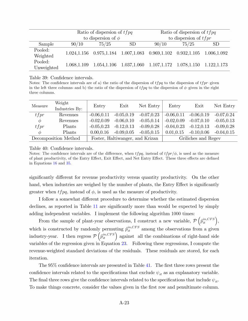
Ratio of dispersion of tfpqto dispersion of φ

Ratio of dispersion of tfpqto dispersion of tfpr

Sample 90/10 75/25 SD 90/10 75/25 SDPooled:Weighted

1.024,1.156 0.975,1.184 1.007,1.083 0.969,1.102 0.932,1.105 1.006,1.092

Pooled:Unweighted

1.068,1.109 1.054,1.106 1.037,1.060 1.107,1.172 1.078,1.150 1.122,1.173

Table 39: Confidence intervals.Notes: The confidence intervals are of a) the ratio of the dispersion of tfpq to the dispersion of tfpr—givenin the left three columns—and b) the ratio of the dispersion of tfpq to the dispersion of φ—given in the rightthree columns.

MeasureWeightIndustries By:

Entry Exit Net Entry Entry Exit Net Entry

tfpr Revenues -0.06,0.11 -0.05,0.19 -0.07,0.23 -0.06,0.11 -0.06,0.19 -0.07,0.24φ Revenues -0.02,0.09 -0.06,0.10 -0.05,0.14 -0.02,0.09 -0.07,0.10 -0.05,0.13

tfpr Plants -0.05,0.23 -0.12,0.13 -0.09,0.28 -0.04,0.23 -0.12,0.13 -0.09,0.28φ Plants 0.00,0.16 -0.09,0.05 -0.05,0.15 0.01,0.15 -0.10,0.06 -0.04,0.15

Decomposition Method Foster, Haltiwanger, and Krizan Griliches and Regev

Table 40: Confidence intervals.Notes: The confidence intervals are of the difference, when tfpq, instead of tfpr/φ, is used as the measureof plant productivity, of the Entry Effect, Exit Effect, and Net Entry Effect. These three effects are definedin Equations 16 and 35.

significantly different for revenue productivity versus quantity productivity. On the other

hand, when industries are weighed by the number of plants, the Entry Effect is significantly

greater when tfpq, instead of φ, is used as the measure of productivity.

I follow a somewhat different procedure to determine whether the estimated dispersion

declines, as reported in Table 11 are significantly more than would be expected by simply

adding independent variables. I implement the following algorithm 1000 times:

From the sample of plant-year observations, I construct a new variable, P(pin,CFSit

),

which is constructed by randomly permuting pin,CFSit among the observations from a given

industry-year. I then regress P(pin,CFSit

)against all the combinations of right-hand side

variables of the regression given in Equation 23. Following these regressions, I compute the

revenue-weighted standard deviations of the residuals. These residuals are stored, for each

iteration.

The 95% confidence intervals are presented in Table 41. The first three rows present the

confidence intervals related to the specifications that exclude ψit as an explanatory variable.

The final three rows give the confidence intervals related to the specifications that include ψit.

To make things concrete, consider the values given in the first row and penultimate column.

A-23

Include DivisionFixed Effects?

No Yes No Yes

Includetfpqit?

No No Yes Yes

SampleSize

Sample

131 Concrete 0.292,0.354 0.342,0.359 0.288,0.352190 Boxes 0.175,0.185 0.184,0.187 0.175,0.185321 Pooled 0.200,0.208 0.206,0.209 0.199,0.207131 Concrete 0.333,0.359 0.286,0.352 0.327,0.359 0.284,0.351190 Boxes 0.184,0.187 0.174,0.185 0.182,0.187 0.174,0.185321 Pooled 0.206,0.209 0.199,0.208 0.205,0.209 0.195,0.207

Table 41: Confidence intervals.Notes: The first three rows present the confidence intervals related to the specifications that exclude ψit asan explanatory variable. The final three rows give the confidence intervals related to the specifications thatinclude ψit.

To construct these two values, I repeatedly regress random permutations of P(pin,CFSit

)against tfpqit, and then store the standard deviation of the residuals from each regression.

The smaller value equals the 2.5-percentile standard deviation, and the larger value equals

the 97.5-percentile standard deviation.

Additional References

White, T. Kirk, Jerome P. Reiter, and Amil Petrin (2012). "Plant-level Productivity and

Imputation of Missing Data in U.S. Census Manufacturing Data." NBER Working

Paper No. 17816.

A-24