material balance reservoir models derived from production data

MATERIAL BALANCE RESERVOIR MODELS DERIVED FROM PRODUCTION DATA

A Dissertation

by

RAFAEL WANDERLEY DE HOLANDA

Submitted to the Office of Graduate and Professional Studies ofTexas A&M University

in partial fulfillment of the requirements for the degree of

DOCTOR OF PHILOSOPHY

Chair of Committee, Eduardo GildinCommittee Members, Thomas A. Blasingame

John KilloughNick Duffield

Head of Department, Jeff Spath

May 2019

Major Subject: Petroleum Engineering

Copyright 2019 Rafael Wanderley de Holanda

ABSTRACT

Rate measurements are the most available data gathered throughout the production life of a

field, and essential to understand reservoir dynamics. In order to gain knowledge quickly from

such data for a massive number of wells, it is important to develop simple reservoir models capable

of history matching and predicting performance using rate measurements, but also incorporating

other types of data (e.g. bottomhole pressures, well locations, completion status), as available.

Even in simplified reservoir models, material balance is a necessary assumption because reservoirs

are limited resources of petroleum.

In this context, capacitance resistance models (CRM’s) comprise a family of material balance

reservoir models that have been applied to primary, secondary and tertiary recovery processes in

conventional reservoirs. CRM’s predict well flow rates based solely on previously observed pro-

duction and injection rates, and producers’ bottomhole pressures (BHP’s); i.e., a geological model

and rock/fluid properties are not required. CRM’s can accelerate the learning curve of the geo-

logical analysis by providing interwell connectivity maps to corroborate features such as sealing

or leaking faults, and high permeability channels. Additionally, oil and water rates are computed

by coupling a fractional flow model to CRM’s, which enables, for example, optimization of water

allocation in mature fields undergoing waterflooding. In this dissertation, a comprehensive review

on CRM’s is presented, summarizing theoretical concepts and relevant aspects for implementation

to field data. Additionally, two case studies are presented distinguishing CRM interwell connec-

tivities from streamline allocation factors.

For unconventional reservoirs, the second Jacobi theta function (θ2 model) is a physics-based

decline curve model proposed, which can be considered an extension of CRM. It accounts for

linear flow and material balance in horizontal multi-stage hydraulically fractured wells. The main

characteristics of pressure diffusion in the porous media are embedded in the functional form, such

that there is a transition from transient to boundary dominated flow and the EUR is always finite.

Analogously to the frequently used Arps hyperbolic, the new model has only three parameters,

ii

where two of them define the decline profile and the third one is a multiplier.

A case study of 992 gas wells in the Barnett shale is presented with probabilistic forecasts of

flowrates and estimated ultimate recovery (EUR) performed in a Bayesian approach. New method-

ologies are proposed for data treatment, uncertainty calibration, and the design of a localized prior

distribution for each well. The results indicate that uncertainty is reliably quantified, and the θ2

model has smaller uncertainty and provides more conservative forecasts than other decline models

commonly used (Arps hyperbolic, Duong and stretched exponential models). Additionally, the

use of previous production of surrounding wells and geospatial data reduces the uncertainty on the

performance of new wells drilled.

iii

DEDICATION

To my beloved wife, family and grandparents.

iv

ACKNOWLEDGMENTS

I would like to thank my wife and my family for their continuous love, support, and fellowship,

which definitely go beyond the extent of this PhD program.

Dr. Maria Alves (Halliburton Engineering Global Programs Office) and Dr. Gildin helped me

to come to Texas A&M University for the first time in 2012, which paved the way to my Masters

of Science and PhD programs. Dr. Gildin has been a great personal and professional advisor over

the years, promoting opportunities for my development, and collaborating in the most challenging

times.

The camaraderie of my friends in the Reservoir Dynamics and Control Research Group and in

Petrobras America Inc. made the good moments more remarkable and the hard moments easier to

navigate, and improved this learning experience. This journey would not be as enjoyable without

them.

I am thankful for the contributions of Dr. Valkó, Dr. Jensen, Dr. Lake and M.S. Shah Kabir.

Our discussions improved my understanding of the problems approached in this dissertation, set-

ting the basis for developments. Dr. Blasingame’s advices and challenging classes are also very

appreciated.

The dissertation committee members, Dr. Gildin, Dr. Blasingame, Dr. Killough and Dr.

Duffield, are acknowledged for their service and advice during this PhD program, including sug-

gestions and revisions of this dissertation.

The staff of Texas A&M University and the Department of Petroleum Engineering are acknowl-

edged for their service, maintaining the campus as a memorable place to study and live. Specially,

Ms. Eleanor Schuler is acknowledged for her assistance in decisive moments.

v

CONTRIBUTORS AND FUNDING SOURCES

Contributors

This dissertation was supported by a committee consisting of Professor Gildin (advisor), Pro-

fessor Blasingame and Professor Killough of the Department of Petroleum Engineering at Texas

A&M University, and Professor Duffield of the Department of Electrical and Computer Engineer-

ing at Texas A&M University.

Professor Jensen of the Chemical and Petroleum Engineering Department at the University

of Calgary, Professor Lake of the Department of Petroleum and Geosystems Engineering at the

University of Texas, and Professor Kabir of the Department of Petroleum Engineering at the Uni-

versity of Houston contributed to chapter 2, engaging in multiple discussions on the content and

structure of the literature review, suggesting references, and proofreading. Professor Jensen also

participated in the analysis of the case studies.

Professor Valkó of the Department of Petroleum Engineering at Texas A&M University taught

me the Wolfram programming language (Mathematica), acquired data for the case studies in chap-

ters 4 and 5, introduced the geometric factor (χ) in the θ2 model, formulated the heuristic rules to

filter “bad data”, reviewed computational codes, and proofread the content of chapters 3-5.

Professor Gildin engaged in countless discussions over the past 7 years, since I was an under-

graduate intern under his supervision. Besides suggesting the scope of work, he is responsible for

maintaining an enthusiastic and collaborative research environment.

All other work conducted for this dissertation was completed by the student independently.

Funding Sources

During this PhD program, five academic semesters were funded by Energi Simulation (for-

merly Foundation CMG) through a graduate research assistantship managed by Texas A&M Engi-

neering Experiment Station (TEES); and two academic semesters were funded by the Department

of Petroleum Engineering through graduate teaching assistantships also managed by TEES.

vi

NOMENCLATURE

1m×n m × n matrix of ones

a linear inequality constraint matrix

a range, [L]

aeq linear equality constraint matrix

aexp exponential fit parameter

av linear weights parameter

A state matrix

A fracture face area, [L2]

Av drainage area of the control volume, [L2]

ACC accuracy

b linear inequality constraint vector

b Arps decline exponent, [dimensionless]

beq linear equality constraint vector

bexp exponential fit parameter

bv linear weights parameter

B input matrix

B number of blocks

ct total compressibility (rock and fluid), [LT 2/M ]

C output matrix

C sill

CCRM CRM number

Ce covariance matrix of the errors, [Nt ×Nt]

vii

D feedforward matrix

Di Arps initial decline rate, [T−1]

E effective oil-solvent viscosity ratio

EUR40 estimated ultimate recovery in 40 years

f interwell connectivity

f ′ fraction of injected flowrate allocated to each layer

fPLT fraction of production flowrate coming from each layer

fo fractional flow of oil

fw fractional flow of water

F cumulative flow capacity

FN false negatives

FNR false negative rate

FP false positives

G(s) transfer function

h distance between attributes, [L]

H heterogeneity factor

I identity matrix

J productivity index, [L4T/M ]

k matrix pemeability, [L2]

Kval Koval factor

lb lower bound vector

L reservoir length, [L]

Ldata ratio of sampled data points to number of parameters

m oil relative permeability exponent

ml lower shifhting parameter

viii

M end-point mobility ratio

n water relative permeability exponent

nMCMC size of Markov chain

N negatives

N normal distribution

Nft number of time steps until end of forecasting window

Ninj number of injectors

NL number of layers

Np cumulative liquid production, [L3]

Npar number of parameters

Nprod number of producers

Nt number of time steps until end of history matching window

NPV net present value

NPV ′ negative predictive valuep pressure, [M/LT 2]

p average pressure of the control volume, [M/LT 2]

pi initial reservoir pressure, [M/LT 2]

pwf producer bottomhole flowing pressure, [M/LT 2]

P positives

Pl(qobs|Ψ) likelihood function

Ppost(Ψ|qobs) posterior distribution

Ppr(Ψ) prior distribution

PDTSP or Q2nd production during the second period, [L3]

PPV positive predictive value

q vector of well flowrate, [Nt × 1]

q producer flowrate, [L3/T ]

ix

qBHP contribution of unknown BHP variations to flowrate, [L3/T ]

q∗i virtual initial flowrate, [L3/T ]

qlim threshold valid production rate, [L3/T ]

qmax maximum well flowrate, [L3/T ]

qp liquid production rate disregarding crossflow, [L3/T ]

Q cumulative production, [L3]

Qc crossflow between layers, [L3/T ]

r discount rate per period

s Laplace variable

S normalized average water saturation

Sor residual oil saturation

Sw water saturation

Swr irreducible water saturation

t time vector, [Nt × 1]

t time, [T ]

T transmissibility, [L4T/M ]

Ts segmented time, [T ]

TN true negatives

TNR true negative rate

TP true positives

TPR true positive rate

u input vector

ub upper bound vector

U uniform distribution

U(s) input vector in Laplace space

x

Ut well trajectories matrix for optimization

v vector of weights, [Nt × 1]

vi ith element of v

Vp total pore volume, [L3]

w injection rate, [L3/T ]

w∗ effective water injected in the control volume, [L3/T ]

wl well horizontal length, [L]

W cumulative water injected, [L3]

W ∗ effective cumulative water injected in the control volume,[L3/T ]

x state vector

x distance from fracture face, [L]

xi lower integration limit for p, [L]

y output vector

Y(s) output vector in Laplace space

z attribute

z attributes average for simple Kriging

zobj history matching objective function

Greek letters

α power-law coefficient for semi-empirical fractional flowmodel

αR acceptance ratio

β power-law exponent for semi-empirical fractional flow model

βm heuristic multiplier

xi

γ variogram

ε inherent error of the production data

η reciprocal characteristic time, [T−1]

θ2 Jacobi theta function no. 2

κ diffusivity constant

λ Kriging weights, [dimensionless]

λvj interwell connectivity between virtual injector and producer

µ fluid viscosity, [M/LT ]

ρ density, [M/L3]

σ standard deviation of the residual

σik covariance between i-th and k-th data points

τ time constant, [T ]

τp time constant for primary production, [T ]

φ matrix porosity, [dimensionless]

Φ cumulative storage capacity

ΦN cumulative distribution function of N (0, 1)

χ geometric factor, [dimensionless]

ψ streamline allocation factor

Ψ vector of model parameters

ω frequency of an event

Ω price

subscripts and superscripts

a aquifer

b b-th block

bf best fit model

xii

cap capacity of the surface facilities

D dimensionless variable

f fracture compartment

i i-th injector

in input

j j-th producer

k k-th time step

low lower bound

m matrix compartment

max maximum

min minimum

n number of points used for Kriging

o oil

obs observed data

ok ordinary Kriging estimate

out output

pred predicted by model

prop proposed model

s sth element in the Markov chain

sk simple Kriging estimate

sv solvent

transf normal score transformed attribute

up upper bound

v number of variogram models summed

w water

xiii

α α-th layer

ν ν-th producer is shut-in

xiv

TABLE OF CONTENTS

Page

ABSTRACT . . . . . . . . . . . . . . . . . . . . . . . . . . . . . . . . . . . . . . . . . . . . . . . . . . . . . . . . . . . . . . . . . . . . . . . . . . . . . . . . . . . . . . . . . ii

DEDICATION . . . . . . . . . . . . . . . . . . . . . . . . . . . . . . . . . . . . . . . . . . . . . . . . . . . . . . . . . . . . . . . . . . . . . . . . . . . . . . . . . . . . . . . iv

ACKNOWLEDGMENTS . . . . . . . . . . . . . . . . . . . . . . . . . . . . . . . . . . . . . . . . . . . . . . . . . . . . . . . . . . . . . . . . . . . . . . . . . . v

CONTRIBUTORS AND FUNDING SOURCES . . . . . . . . . . . . . . . . . . . . . . . . . . . . . . . . . . . . . . . . . . . . . . . . . vi

NOMENCLATURE . . . . . . . . . . . . . . . . . . . . . . . . . . . . . . . . . . . . . . . . . . . . . . . . . . . . . . . . . . . . . . . . . . . . . . . . . . . . . . . . . vii

TABLE OF CONTENTS . . . . . . . . . . . . . . . . . . . . . . . . . . . . . . . . . . . . . . . . . . . . . . . . . . . . . . . . . . . . . . . . . . . . . . . . . . . xv

LIST OF FIGURES . . . . . . . . . . . . . . . . . . . . . . . . . . . . . . . . . . . . . . . . . . . . . . . . . . . . . . . . . . . . . . . . . . . . . . . . . . . . . . . . . xix

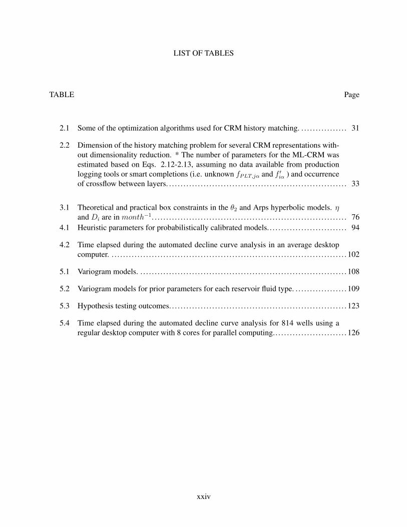
LIST OF TABLES. . . . . . . . . . . . . . . . . . . . . . . . . . . . . . . . . . . . . . . . . . . . . . . . . . . . . . . . . . . . . . . . . . . . . . . . . . . . . . . . . . .xxiv

1. INTRODUCTION. . . . . . . . . . . . . . . . . . . . . . . . . . . . . . . . . . . . . . . . . . . . . . . . . . . . . . . . . . . . . . . . . . . . . . . . . . . . . . . 1

1.1 Literature review . . . . . . . . . . . . . . . . . . . . . . . . . . . . . . . . . . . . . . . . . . . . . . . . . . . . . . . . . . . . . . . . . . . . . . . . . . 21.1.1 Capacitance resistance models (CRM’s) for conventional reservoirs . . . . . . . . . 21.1.2 Simple models for unconventional reservoirs . . . . . . . . . . . . . . . . . . . . . . . . . . . . . . . . . . . 6

1.2 Problem statement and significance . . . . . . . . . . . . . . . . . . . . . . . . . . . . . . . . . . . . . . . . . . . . . . . . . . . . . . 111.3 Objectives . . . . . . . . . . . . . . . . . . . . . . . . . . . . . . . . . . . . . . . . . . . . . . . . . . . . . . . . . . . . . . . . . . . . . . . . . . . . . . . . . 12

1.3.1 Primary objectives . . . . . . . . . . . . . . . . . . . . . . . . . . . . . . . . . . . . . . . . . . . . . . . . . . . . . . . . . . . . . . . . 121.3.2 Secondary objectives . . . . . . . . . . . . . . . . . . . . . . . . . . . . . . . . . . . . . . . . . . . . . . . . . . . . . . . . . . . . . 13

1.4 Outline . . . . . . . . . . . . . . . . . . . . . . . . . . . . . . . . . . . . . . . . . . . . . . . . . . . . . . . . . . . . . . . . . . . . . . . . . . . . . . . . . . . . . 13

2. CAPACITANCE RESISTANCE MODELS . . . . . . . . . . . . . . . . . . . . . . . . . . . . . . . . . . . . . . . . . . . . . . . . . . . 15

2.1 Underlying concepts: material balance and deliverability . . . . . . . . . . . . . . . . . . . . . . . . . . . . . . 152.2 Reservoir control volumes . . . . . . . . . . . . . . . . . . . . . . . . . . . . . . . . . . . . . . . . . . . . . . . . . . . . . . . . . . . . . . . . 16

2.2.1 CRMT: single tank representation . . . . . . . . . . . . . . . . . . . . . . . . . . . . . . . . . . . . . . . . . . . . . . . 162.2.2 CRMP: producer based representation . . . . . . . . . . . . . . . . . . . . . . . . . . . . . . . . . . . . . . . . . . 182.2.3 CRMIP: injector-producer pair based representation . . . . . . . . . . . . . . . . . . . . . . . . . . . 192.2.4 CRM-block: blocks in series representation . . . . . . . . . . . . . . . . . . . . . . . . . . . . . . . . . . . . 202.2.5 Multilayer CRM: blocks in parallel representation . . . . . . . . . . . . . . . . . . . . . . . . . . . . . 21

2.3 CRM parameters physical meaning . . . . . . . . . . . . . . . . . . . . . . . . . . . . . . . . . . . . . . . . . . . . . . . . . . . . . . 232.3.1 Connectivities. . . . . . . . . . . . . . . . . . . . . . . . . . . . . . . . . . . . . . . . . . . . . . . . . . . . . . . . . . . . . . . . . . . . . 23

2.3.1.1 Aquifer-producer connectivity . . . . . . . . . . . . . . . . . . . . . . . . . . . . . . . . . . . . . . . . 262.3.1.2 Connectivity interpretation within a flood management perspective 27

xv

2.3.2 Time constants . . . . . . . . . . . . . . . . . . . . . . . . . . . . . . . . . . . . . . . . . . . . . . . . . . . . . . . . . . . . . . . . . . . . 282.4 CRM for primary production . . . . . . . . . . . . . . . . . . . . . . . . . . . . . . . . . . . . . . . . . . . . . . . . . . . . . . . . . . . . . 282.5 CRM history matching . . . . . . . . . . . . . . . . . . . . . . . . . . . . . . . . . . . . . . . . . . . . . . . . . . . . . . . . . . . . . . . . . . . . 29

2.5.1 Dimensionality reduction . . . . . . . . . . . . . . . . . . . . . . . . . . . . . . . . . . . . . . . . . . . . . . . . . . . . . . . . 322.5.2 Alternative CRM formulations . . . . . . . . . . . . . . . . . . . . . . . . . . . . . . . . . . . . . . . . . . . . . . . . . . 34

2.5.2.1 Matching cumulative production: the integrated capacitance re-sistance model (ICRM) . . . . . . . . . . . . . . . . . . . . . . . . . . . . . . . . . . . . . . . . . . . . . . . 34

2.5.2.2 Unmeasured BHP variations: segmented CRM .. . . . . . . . . . . . . . . . . . . . 352.5.2.3 Changes in well status: compensated CRM.. . . . . . . . . . . . . . . . . . . . . . . . . 35

2.6 CRM sensitivity to data quality and uncertainty analysis . . . . . . . . . . . . . . . . . . . . . . . . . . . . . . . 362.7 Fractional flow models . . . . . . . . . . . . . . . . . . . . . . . . . . . . . . . . . . . . . . . . . . . . . . . . . . . . . . . . . . . . . . . . . . . . 38

2.7.1 Buckley-Leverett adapted to CRM .. . . . . . . . . . . . . . . . . . . . . . . . . . . . . . . . . . . . . . . . . . . . . 392.7.2 Semi-empirical power-law fractional flow model . . . . . . . . . . . . . . . . . . . . . . . . . . . . . . . 402.7.3 Koval fractional flow model . . . . . . . . . . . . . . . . . . . . . . . . . . . . . . . . . . . . . . . . . . . . . . . . . . . . . 42

2.8 CRM enhanced oil recovery . . . . . . . . . . . . . . . . . . . . . . . . . . . . . . . . . . . . . . . . . . . . . . . . . . . . . . . . . . . . . . 442.8.1 CO2 flooding . . . . . . . . . . . . . . . . . . . . . . . . . . . . . . . . . . . . . . . . . . . . . . . . . . . . . . . . . . . . . . . . . . . . . . 462.8.2 Water alternating gas (WAG) . . . . . . . . . . . . . . . . . . . . . . . . . . . . . . . . . . . . . . . . . . . . . . . . . . . . 472.8.3 Simultaneous water and gas (SWAG) . . . . . . . . . . . . . . . . . . . . . . . . . . . . . . . . . . . . . . . . . . . 472.8.4 Hydrocarbon gas and nitrogen injection. . . . . . . . . . . . . . . . . . . . . . . . . . . . . . . . . . . . . . . . . 472.8.5 Isothermal EOR (solvent flooding, surfactant-polymer flooding, polymer

flooding, alkaline-surfactant-polymer flooding) . . . . . . . . . . . . . . . . . . . . . . . . . . . . . . . . 482.8.6 Hot waterflooding . . . . . . . . . . . . . . . . . . . . . . . . . . . . . . . . . . . . . . . . . . . . . . . . . . . . . . . . . . . . . . . . 482.8.7 Geothermal reservoirs . . . . . . . . . . . . . . . . . . . . . . . . . . . . . . . . . . . . . . . . . . . . . . . . . . . . . . . . . . . . 48

2.9 CRM and geomechanical effects . . . . . . . . . . . . . . . . . . . . . . . . . . . . . . . . . . . . . . . . . . . . . . . . . . . . . . . . . 492.10 CRM field development optimization . . . . . . . . . . . . . . . . . . . . . . . . . . . . . . . . . . . . . . . . . . . . . . . . . . . . 50

2.10.1 Well control . . . . . . . . . . . . . . . . . . . . . . . . . . . . . . . . . . . . . . . . . . . . . . . . . . . . . . . . . . . . . . . . . . . . . . . 502.10.2 Well placement . . . . . . . . . . . . . . . . . . . . . . . . . . . . . . . . . . . . . . . . . . . . . . . . . . . . . . . . . . . . . . . . . . . 53

2.11 CRM in a control systems perspective . . . . . . . . . . . . . . . . . . . . . . . . . . . . . . . . . . . . . . . . . . . . . . . . . . . 542.12 Case studies comparing CRM interwell connectivities with streamline allocation

factors . . . . . . . . . . . . . . . . . . . . . . . . . . . . . . . . . . . . . . . . . . . . . . . . . . . . . . . . . . . . . . . . . . . . . . . . . . . . . . . . . . . . . . 572.13 Unresolved issues and suggestions for future research . . . . . . . . . . . . . . . . . . . . . . . . . . . . . . . . . . 61

2.13.1 Gas content of reservoir fluids . . . . . . . . . . . . . . . . . . . . . . . . . . . . . . . . . . . . . . . . . . . . . . . . . . . 622.13.2 Rate measurements . . . . . . . . . . . . . . . . . . . . . . . . . . . . . . . . . . . . . . . . . . . . . . . . . . . . . . . . . . . . . . . 632.13.3 Well-orientation and completion type . . . . . . . . . . . . . . . . . . . . . . . . . . . . . . . . . . . . . . . . . . . 632.13.4 Time-varying behavior of the CRM parameters . . . . . . . . . . . . . . . . . . . . . . . . . . . . . . . . 642.13.5 CRM coupling with fractional flow models and well control optimization . . . 642.13.6 Unconventional reservoirs . . . . . . . . . . . . . . . . . . . . . . . . . . . . . . . . . . . . . . . . . . . . . . . . . . . . . . . 65

3. A PHYSICS-BASED DECLINE MODEL FOR UNCONVENTIONAL RESERVOIRS. . . 67

3.1 Physics: Jacobi theta function no. 2 as a decline curve model . . . . . . . . . . . . . . . . . . . . . . . . . . 673.1.1 Model derivation. . . . . . . . . . . . . . . . . . . . . . . . . . . . . . . . . . . . . . . . . . . . . . . . . . . . . . . . . . . . . . . . . . 673.1.2 Subcases and extensions of the θ2 model. . . . . . . . . . . . . . . . . . . . . . . . . . . . . . . . . . . . . . . . 71

3.1.2.1 Wattenbarger et al. [1998] . . . . . . . . . . . . . . . . . . . . . . . . . . . . . . . . . . . . . . . . . . . . 713.1.2.2 Double-porosity model [Ogunyomi et al., 2016] . . . . . . . . . . . . . . . . . . . . 71

xvi

3.1.3 Comparison with the Arps decline model . . . . . . . . . . . . . . . . . . . . . . . . . . . . . . . . . . . . . . . 723.2 History matching . . . . . . . . . . . . . . . . . . . . . . . . . . . . . . . . . . . . . . . . . . . . . . . . . . . . . . . . . . . . . . . . . . . . . . . . . . 763.3 Statistics: uncertainty quantification . . . . . . . . . . . . . . . . . . . . . . . . . . . . . . . . . . . . . . . . . . . . . . . . . . . . . 77

3.3.1 Bayes theorem . . . . . . . . . . . . . . . . . . . . . . . . . . . . . . . . . . . . . . . . . . . . . . . . . . . . . . . . . . . . . . . . . . . . 773.3.2 Markov chain Monte Carlo (MCMC) algorithm . . . . . . . . . . . . . . . . . . . . . . . . . . . . . . . . 783.3.3 The roles of the prior distribution and the likelihood function . . . . . . . . . . . . . . . . . 81

3.4 Heuristics: treating the bad data . . . . . . . . . . . . . . . . . . . . . . . . . . . . . . . . . . . . . . . . . . . . . . . . . . . . . . . . . . 843.4.1 Tuning the heuristics for uncertainty calibration . . . . . . . . . . . . . . . . . . . . . . . . . . . . . . . . 86

4. BARNETT CASE STUDY PART 1: PROBABILISTIC CALIBRATION AND COM-PARISON OF THE θ2 WITH OTHER DECLINE MODELS . . . . . . . . . . . . . . . . . . . . . . . . . . . . . . . . 89

4.1 Describing the dataset: 992 gas wells from the Barnett shale. . . . . . . . . . . . . . . . . . . . . . . . . . . 894.2 Selecting the prior distribution . . . . . . . . . . . . . . . . . . . . . . . . . . . . . . . . . . . . . . . . . . . . . . . . . . . . . . . . . . . 914.3 Probabilistic calibration . . . . . . . . . . . . . . . . . . . . . . . . . . . . . . . . . . . . . . . . . . . . . . . . . . . . . . . . . . . . . . . . . . . 934.4 EUR estimates: comparison of the θ2 with other decline models . . . . . . . . . . . . . . . . . . . . . . 964.5 Examples of the θ2 production forecast . . . . . . . . . . . . . . . . . . . . . . . . . . . . . . . . . . . . . . . . . . . . . . . . . . 984.6 The impact of the liquid content on χ . . . . . . . . . . . . . . . . . . . . . . . . . . . . . . . . . . . . . . . . . . . . . . . . . . . . 1004.7 Discussion . . . . . . . . . . . . . . . . . . . . . . . . . . . . . . . . . . . . . . . . . . . . . . . . . . . . . . . . . . . . . . . . . . . . . . . . . . . . . . . . . 101

5. BARNETT CASE STUDY PART 2: THE DESIGN OF A LOCALIZED PRIOR DIS-TRIBUTION. . . . . . . . . . . . . . . . . . . . . . . . . . . . . . . . . . . . . . . . . . . . . . . . . . . . . . . . . . . . . . . . . . . . . . . . . . . . . . . . . . . . . 105

5.1 Describing the dataset: 814 gas wells from the Barnett shale. . . . . . . . . . . . . . . . . . . . . . . . . . . 1055.2 The design of a localized prior distribution . . . . . . . . . . . . . . . . . . . . . . . . . . . . . . . . . . . . . . . . . . . . . 106

5.2.1 Preliminary geostatistical concepts . . . . . . . . . . . . . . . . . . . . . . . . . . . . . . . . . . . . . . . . . . . . . 1075.2.1.1 Variogram models . . . . . . . . . . . . . . . . . . . . . . . . . . . . . . . . . . . . . . . . . . . . . . . . . . . . . 1075.2.1.2 Localized simple Kriging . . . . . . . . . . . . . . . . . . . . . . . . . . . . . . . . . . . . . . . . . . . . . 110

5.2.2 Prior distribution. . . . . . . . . . . . . . . . . . . . . . . . . . . . . . . . . . . . . . . . . . . . . . . . . . . . . . . . . . . . . . . . . . 1115.2.2.1 General prior by reservoir fluid-type . . . . . . . . . . . . . . . . . . . . . . . . . . . . . . . . . 1125.2.2.2 Localized prior . . . . . . . . . . . . . . . . . . . . . . . . . . . . . . . . . . . . . . . . . . . . . . . . . . . . . . . . 113

5.3 Results . . . . . . . . . . . . . . . . . . . . . . . . . . . . . . . . . . . . . . . . . . . . . . . . . . . . . . . . . . . . . . . . . . . . . . . . . . . . . . . . . . . . . 1155.3.1 Behavior of the localized priors. . . . . . . . . . . . . . . . . . . . . . . . . . . . . . . . . . . . . . . . . . . . . . . . . . 1155.3.2 Comparison between single and localized priors . . . . . . . . . . . . . . . . . . . . . . . . . . . . . . . 1155.3.3 The localized prior as an indicator for infill drilling locations . . . . . . . . . . . . . . . . . 122

5.4 Discussion . . . . . . . . . . . . . . . . . . . . . . . . . . . . . . . . . . . . . . . . . . . . . . . . . . . . . . . . . . . . . . . . . . . . . . . . . . . . . . . . . 124

6. CONCLUSIONS . . . . . . . . . . . . . . . . . . . . . . . . . . . . . . . . . . . . . . . . . . . . . . . . . . . . . . . . . . . . . . . . . . . . . . . . . . . . . . . . 127

6.1 Capacitance resistance models for conventional reservoirs . . . . . . . . . . . . . . . . . . . . . . . . . . . . . 1276.2 θ2 model for automated probabilistic decline curve analysis of unconventional

reservoirs . . . . . . . . . . . . . . . . . . . . . . . . . . . . . . . . . . . . . . . . . . . . . . . . . . . . . . . . . . . . . . . . . . . . . . . . . . . . . . . . . . 1286.3 The localized prior distribution approach . . . . . . . . . . . . . . . . . . . . . . . . . . . . . . . . . . . . . . . . . . . . . . . . 1296.4 Future works. . . . . . . . . . . . . . . . . . . . . . . . . . . . . . . . . . . . . . . . . . . . . . . . . . . . . . . . . . . . . . . . . . . . . . . . . . . . . . . 130

REFERENCES . . . . . . . . . . . . . . . . . . . . . . . . . . . . . . . . . . . . . . . . . . . . . . . . . . . . . . . . . . . . . . . . . . . . . . . . . . . . . . . . . . . . . . 132

xvii

APPENDIX A. DERIVATION OF PRESSURE SOLUTION FOR 1-D LINEAR RESER-VOIR . . . . . . . . . . . . . . . . . . . . . . . . . . . . . . . . . . . . . . . . . . . . . . . . . . . . . . . . . . . . . . . . . . . . . . . . . . . . . . . . . . . . . . . . . . . . . 149

APPENDIX B. PROOF OF FINITE EUR FOR THE θ2 MODEL. . . . . . . . . . . . . . . . . . . . . . . . . . . . . . . 154

APPENDIX C. ADDITIONAL FIGURES. . . . . . . . . . . . . . . . . . . . . . . . . . . . . . . . . . . . . . . . . . . . . . . . . . . . . . . . 156

APPENDIX D. ESTIMATION OF PROBABILITY DISTRIBUTION FORQMAX AT NEWLOCATIONS . . . . . . . . . . . . . . . . . . . . . . . . . . . . . . . . . . . . . . . . . . . . . . . . . . . . . . . . . . . . . . . . . . . . . . . . . . . . . . . . . . . . 161

xviii

LIST OF FIGURES

FIGURE Page

1.1 Types of reservoir models (adapted from Gildin and King, 2013). . . . . . . . . . . . . . . . . . . . . . 1

1.2 The design of capacitor resistor networks for predicting the behavior of strong-water drive reservoirs: (a) Network proposed by Bruce [1943]; (b) Inside view ofmodel applied to Saudi Arabian fields, it was a mesh of 2,501 capacitors and 4,900resistors [Wahl et al., 1962]. . . . . . . . . . . . . . . . . . . . . . . . . . . . . . . . . . . . . . . . . . . . . . . . . . . . . . . . . . . . . . . 3

1.3 More than 260 public-domain documents concerning capacitance resistance mod-els (CRM’s) or their applications have appeared since 2006. Source: GoogleScholar. 2016–18* indicates publications through September 29, 2018.. . . . . . . . . . . . . . . 5

2.1 Reservoir control volumes for CRM representations: (a) single tank (CRMT); (b)producer based (CRMP); (c) injector-producer pair based (CRMIP); (d) blocks inseries (CRM-block); (e) multi-layer or blocks in parallel (ML-CRM). . . . . . . . . . . . . . . . . 17

2.2 (a) CRM response to a sequence of step injection signals for several values of in-terwell connectivity. (b) Physical meaning of time constants: percent of stationaryresponse achieved at a specific dimensionless time. . . . . . . . . . . . . . . . . . . . . . . . . . . . . . . . . . . . . . 24

2.3 (a) Example of modified Brooks and Corey [1964] relative permeability model. (b)Buckley-Leverett prediction of the flood-front advance. (c) Water-cut sensitivityto parameters in Eq. 2.29; the title of each subplot indicates which parameter ischanging with values shown in the legends (base case: w = 1 bbl/day, Vp = 1bbl, Swr = 0.2, Sor = 0.2, M = 0.33, m = 3, n = 2; observation: w and Vp arenormalized for the base case). . . . . . . . . . . . . . . . . . . . . . . . . . . . . . . . . . . . . . . . . . . . . . . . . . . . . . . . . . . . . 41

2.4 (a) Example of history matching the late time WOR with the power-law relations(these four producers are in the reservoir shown in Fig. 2.6a). Water-cut sensitivityto parameters of the semi-empirical fractional flow model: (b) αj , and (c) βj . . . . . . . . . 42

2.5 (a) WOR resulting from history matching the early and late time water-cut withthe Koval fractional flow model (these four producers are in the reservoir shown inFig. 2.6a). Water-cut sensitivity to parameters of the Koval fractional flow model:(b) Vp, and (c) Kval. . . . . . . . . . . . . . . . . . . . . . . . . . . . . . . . . . . . . . . . . . . . . . . . . . . . . . . . . . . . . . . . . . . . . . . . 44

2.6 (a) Fluvial environment reservoir based on the SPE-10 model, previously describedin Holanda [2015]. (b) Flow capacity plot for four producers. ‘PROD5’ is the mostefficient producer in terms of sweep efficiency while ‘PROD3’ is the least efficientone, which can potentially improve through EOR processes. . . . . . . . . . . . . . . . . . . . . . . . . . . . 46

xix

2.7 Input-output representation of the reservoir system. . . . . . . . . . . . . . . . . . . . . . . . . . . . . . . . . . . . . 55

2.8 Block diagram representation of state-space equations. . . . . . . . . . . . . . . . . . . . . . . . . . . . . . . . . . 55

2.9 Maps for CRMIP connectivity (left) and median streamline allocation factor (right).The blue line depicts the low permeability barrier (kh = 1 md), the reservoir hori-zontal permeability (kh) is 200 md. . . . . . . . . . . . . . . . . . . . . . . . . . . . . . . . . . . . . . . . . . . . . . . . . . . . . . . 58

2.10 Comparison between fij and ψij(t): good fit (left), largest difference (center) andlargest variance for ψij (right). . . . . . . . . . . . . . . . . . . . . . . . . . . . . . . . . . . . . . . . . . . . . . . . . . . . . . . . . . . . 58

2.11 Maps for CRMIP connectivity (left) and median streamline allocation factor (right).The contours show the log(kh×h(md×ft)) values, which represents the reservoirheterogeneity. . . . . . . . . . . . . . . . . . . . . . . . . . . . . . . . . . . . . . . . . . . . . . . . . . . . . . . . . . . . . . . . . . . . . . . . . . . . . . . 60

2.12 Comparison between fij and ψij(t): good fit (left), largest difference (center) andlargest variance for ψij (right). . . . . . . . . . . . . . . . . . . . . . . . . . . . . . . . . . . . . . . . . . . . . . . . . . . . . . . . . . . . 60

3.1 a) Representation of a horizontal well with evenly spaced hydraulic fractures. Thedashed red box indicates the symmetric element considered in the derivation ofthe θ2 model. b) Top view of the symmetric element with diffusivity equationand initial and boundary conditions. The hydraulic fractures are assumed to beinfinitely conductive. . . . . . . . . . . . . . . . . . . . . . . . . . . . . . . . . . . . . . . . . . . . . . . . . . . . . . . . . . . . . . . . . . . . . . 68

3.2 The double-porosity model approximation in terms of θ2 functions. q∗i is inmcf/monthand η is in month−1. . . . . . . . . . . . . . . . . . . . . . . . . . . . . . . . . . . . . . . . . . . . . . . . . . . . . . . . . . . . . . . . . . . . . . 72

3.3 Sensitivity to: (a) b and (b) Di parameters in the Arps hyperbolic model. In eachplot one of the parameters is fixed at the median value of the best fit solutions for the992 Barnett gas wells presented in chapter 4. Di is in month−1 and qD(t) = q(t)/q∗i . 73

3.4 Sensitivity to: (a) η and (b) χ parameters in the θ2 model. In each plot one ofthe parameters is fixed at the median value of the best fit solutions for the 992Barnett gas wells presented in chapter 4. The half slope indicates transient flowand the exponential decline indicates boundary dominated flow. η is in month−1

and qD(t) = q(t)/q∗i . . . . . . . . . . . . . . . . . . . . . . . . . . . . . . . . . . . . . . . . . . . . . . . . . . . . . . . . . . . . . . . . . . . . . . 75

3.5 Best fit solutions for the 992 Barnett gas wells with the θ2 model: (a) distributionin the χ vs. η space, the yellow area depicts the linear constraint; (b) relationshipbetween q∗i and qmax. . . . . . . . . . . . . . . . . . . . . . . . . . . . . . . . . . . . . . . . . . . . . . . . . . . . . . . . . . . . . . . . . . . . . . . 77

3.6 Bayes theorem idea applied to well 8 (API #: 42121329920000) with the newworkflow and model. Normalized probability distribution function values are de-picted by the color scale in the 3 parameter solution space for: (a) prior, (b) likeli-hood, (c) posterior. η is in month−1 and q∗i is in mcf/month. . . . . . . . . . . . . . . . . . . . . . . . . 79

xx

3.7 Application of the Bayes theorem to the θ2 model with two different prior distri-butions. The likelihood function considers the first 12 months of production datafrom well API#4212133349. All probability distribution functions are normalizedby their maximum values and depicted by the color scale. η is in month−1 and q∗iis in mcf/month. . . . . . . . . . . . . . . . . . . . . . . . . . . . . . . . . . . . . . . . . . . . . . . . . . . . . . . . . . . . . . . . . . . . . . . . . 82

3.8 Application of the Bayes theorem to the θ2 model considering the same prior dis-tribution, but different lengths of production history for the likelihood function ofwell API#4212133349. All probability distribution functions are normalized bytheir maximum values and depicted by the color scale. η is in month−1 and q∗i isin mcf/month. . . . . . . . . . . . . . . . . . . . . . . . . . . . . . . . . . . . . . . . . . . . . . . . . . . . . . . . . . . . . . . . . . . . . . . . . . . 83

3.9 Best fit solutions of the θ2 model using heuristic rules to filter the data. . . . . . . . . . . . . . . . 86

3.10 Base case, no heuristic rules applied, i.e. av = 0, bv = 1, ml = 1 and βm = 1. Theuncertainty is not calibrated. . . . . . . . . . . . . . . . . . . . . . . . . . . . . . . . . . . . . . . . . . . . . . . . . . . . . . . . . . . . . . . 88

3.11 Case with adjusted heuristic rules for probabilistic calibration. . . . . . . . . . . . . . . . . . . . . . . . . 88

4.1 Wellhead locations of the gas wells in the Barnett shale that were selected foranalysis. Marker types indicate period of beginning of production. . . . . . . . . . . . . . . . . . . . 90

4.2 (a) Histogram of horizontal length of the selected wells, which is estimated as thedistance between the coordinates of the wellhead and toe of the wells. (b) Verticaldepth of the horizontal wells, which is estimated as the difference between the totaldepth (TD) and horizontal length. . . . . . . . . . . . . . . . . . . . . . . . . . . . . . . . . . . . . . . . . . . . . . . . . . . . . . . . . 91

4.3 Fluid classification based on initial producing gas-liquid ratio (GLRi) for 992 wellsin the Barnett shale. . . . . . . . . . . . . . . . . . . . . . . . . . . . . . . . . . . . . . . . . . . . . . . . . . . . . . . . . . . . . . . . . . . . . . . . 92

4.4 Reservoir fluid-type classification based on initial producing gas-liquid ratio (GLRi,in scf/STB ). . . . . . . . . . . . . . . . . . . . . . . . . . . . . . . . . . . . . . . . . . . . . . . . . . . . . . . . . . . . . . . . . . . . . . . . . . . . . . 92

4.5 Prior distributions for the parameters of the θ2 model. It is assumed that the θ2

parameters are independent of each other. . . . . . . . . . . . . . . . . . . . . . . . . . . . . . . . . . . . . . . . . . . . . . . . 93

4.6 Prior distributions for the parameters of the Arps hyperbolic model. It is assumedthat the θ2 parameters are independent of each other. . . . . . . . . . . . . . . . . . . . . . . . . . . . . . . . . . . . 94

4.7 Average production during the second period (PDTSP) for probabilistic and bestfit models compared with the production data for hindcasts. . . . . . . . . . . . . . . . . . . . . . . . . . . . 95

4.8 The probabilistic calibration is necessary for reliable uncertainty assessment. Un-certainty reduces as more data is acquired for calibrated models. . . . . . . . . . . . . . . . . . . . . . . 96

4.9 Comparison of cumulative production during 40 years for probabilistically cali-brated models. . . . . . . . . . . . . . . . . . . . . . . . . . . . . . . . . . . . . . . . . . . . . . . . . . . . . . . . . . . . . . . . . . . . . . . . . . . . . . 97

xxi

4.10 Comparison of cumulative production during 40 years for best fit solutions of theθ2, stretched exponential, Duong and Arps hyperbolic models. Heuristic parame-ters: av = 1.747, ml = 0.954, βm = 0.003. . . . . . . . . . . . . . . . . . . . . . . . . . . . . . . . . . . . . . . . . . . . . . . 98

4.11 Prediction from history matched and probabilistic θ2 models considering the first24 months of production and comparing prediction with the actual production history. 99

4.12 θ2 models compared to field data showing evidence of transition to boundary dom-inated flow and initial production buildup.. . . . . . . . . . . . . . . . . . . . . . . . . . . . . . . . . . . . . . . . . . . . . . . 100

4.13 Histograms for the χ parameter considering the best-fit solutions for the full gasproduction history and organized by reservoir fluid type. . . . . . . . . . . . . . . . . . . . . . . . . . . . . . . . 101

5.1 Histograms of the best fit history matched model parameters and single prior para-metric distributions (blue line) obtained for the 814 gas wells. . . . . . . . . . . . . . . . . . . . . . . . . 106

5.2 Maps with the P50 estimates of θ2 parameters in the case of a single prior assignedto all wells. Spatial patterns are observed, which reflect on local similarities inthe well performance. η−1 is in months. The locations of the Newark East field(shaded area), Muenster arch and Viola Simpson pinch-out were obtained fromPollastro et al. [2003]. The red dashed line show the location of known faults,and the bicolored lines indicate the limits between reservoir-fluid type windowsaccording to Fig. 4.4. . . . . . . . . . . . . . . . . . . . . . . . . . . . . . . . . . . . . . . . . . . . . . . . . . . . . . . . . . . . . . . . . . . . . 107

5.3 Example of normal score transform. . . . . . . . . . . . . . . . . . . . . . . . . . . . . . . . . . . . . . . . . . . . . . . . . . . . . . 109

5.4 Variogram models matched to the P50 estimates for each reservoir fluid type. . . . . . . . . 110

5.5 Workflow for the development of a localized prior. . . . . . . . . . . . . . . . . . . . . . . . . . . . . . . . . . . . . . 114

5.6 Maps with the P50 estimates of θ2 parameters in the case of localized priors. Thecolor scales for the maps are the same as in Fig. 5.2. η−1 is in months. Thelocations of the Newark East field (shaded area), Muenster arch and Viola Simpsonpinch-out were obtained from Pollastro et al. [2003]. The red dashed line showthe location of known faults, and the bicolored lines indicate the limits betweenreservoir-fluid type windows according to Fig. 4.4. . . . . . . . . . . . . . . . . . . . . . . . . . . . . . . . . . . . . 117

5.7 Average production during the second period (PDTSP) for best fit and probabilisticmodels in the cases of single and localized priors. . . . . . . . . . . . . . . . . . . . . . . . . . . . . . . . . . . . . . . 118

5.8 Uncertainty quantification for: (a) all of the wells; (b) all wells of each reservoirfluid-type. Localized prior case is represented by solid line and the single prior bydashed line. . . . . . . . . . . . . . . . . . . . . . . . . . . . . . . . . . . . . . . . . . . . . . . . . . . . . . . . . . . . . . . . . . . . . . . . . . . . . . . . 118

5.9 Uncertainty quantification for dry gas wells subdivided in groups by initial produc-tion date. Comparison of the localized and single prior cases. . . . . . . . . . . . . . . . . . . . . . . . . . 119

xxii

5.10 Diagnostic plot to assess the uncertainty quantification. . . . . . . . . . . . . . . . . . . . . . . . . . . . . . . . . 120

5.11 Plots comparing probabilistic forecasts with localized and single priors for 9 wells,using 3 years of production history. . . . . . . . . . . . . . . . . . . . . . . . . . . . . . . . . . . . . . . . . . . . . . . . . . . . . . 121

5.12 Maps of P50 estimates for the EUR40 normalized by the horizontal length (inmcf/ft) using (a) single prior and (b) localized priors.. . . . . . . . . . . . . . . . . . . . . . . . . . . . . . . . . . . 122

C.1 General prior of each reservoir fluid type, and localized prior of the wells in eachclass. . . . . . . . . . . . . . . . . . . . . . . . . . . . . . . . . . . . . . . . . . . . . . . . . . . . . . . . . . . . . . . . . . . . . . . . . . . . . . . . . . . . . . . 156

C.2 Analysis of the localized prior as an indicator for infill drilling locations in the caseof known qmax. Five years P50 forecasts from localized prior compared to actualproduction for wells starting production between September 2010 and February2013. The localized prior forecasts do not consider the production history of thewells. ALR is the average log residual: ALR = 1

N

∑√(logQobs − logQpred)2. . . . . 157

C.3 Analysis of the localized prior as an indicator for infill drilling locations in the caseof unknown qmax. Five years P50 forecasts from localized prior compared to actualproduction for wells starting production between September 2010 and February2013. The localized prior forecasts do not consider the production history of thewells. ALR is the average log residual: ALR = 1

N

∑√(logQobs − logQpred)2. . . . 158

C.4 Hypothesis testing results (true positive rates and positive predictive values) forlocalized prior of wells starting production between September 2010 and February2013. . . . . . . . . . . . . . . . . . . . . . . . . . . . . . . . . . . . . . . . . . . . . . . . . . . . . . . . . . . . . . . . . . . . . . . . . . . . . . . . . . . . . . . 159

C.5 Hypothesis testing results (true negative rates, negative predictive values and accu-racy) for localized prior of wells starting production between September 2010 andFebruary 2013. . . . . . . . . . . . . . . . . . . . . . . . . . . . . . . . . . . . . . . . . . . . . . . . . . . . . . . . . . . . . . . . . . . . . . . . . . . . 160

xxiii

LIST OF TABLES

TABLE Page

2.1 Some of the optimization algorithms used for CRM history matching. . . . . . . . . . . . . . . . . 31

2.2 Dimension of the history matching problem for several CRM representations with-out dimensionality reduction. * The number of parameters for the ML-CRM wasestimated based on Eqs. 2.12-2.13, assuming no data available from productionlogging tools or smart completions (i.e. unknown fPLT,jα and f ′iα ) and occurrenceof crossflow between layers. . . . . . . . . . . . . . . . . . . . . . . . . . . . . . . . . . . . . . . . . . . . . . . . . . . . . . . . . . . . . . . 33

3.1 Theoretical and practical box constraints in the θ2 and Arps hyperbolic models. ηand Di are in month−1. . . . . . . . . . . . . . . . . . . . . . . . . . . . . . . . . . . . . . . . . . . . . . . . . . . . . . . . . . . . . . . . . . . . 76

4.1 Heuristic parameters for probabilistically calibrated models. . . . . . . . . . . . . . . . . . . . . . . . . . . . 94

4.2 Time elapsed during the automated decline curve analysis in an average desktopcomputer. . . . . . . . . . . . . . . . . . . . . . . . . . . . . . . . . . . . . . . . . . . . . . . . . . . . . . . . . . . . . . . . . . . . . . . . . . . . . . . . . . . 102

5.1 Variogram models. . . . . . . . . . . . . . . . . . . . . . . . . . . . . . . . . . . . . . . . . . . . . . . . . . . . . . . . . . . . . . . . . . . . . . . . . 108

5.2 Variogram models for prior parameters for each reservoir fluid type. . . . . . . . . . . . . . . . . . . 109

5.3 Hypothesis testing outcomes. . . . . . . . . . . . . . . . . . . . . . . . . . . . . . . . . . . . . . . . . . . . . . . . . . . . . . . . . . . . . . 123

5.4 Time elapsed during the automated decline curve analysis for 814 wells using aregular desktop computer with 8 cores for parallel computing.. . . . . . . . . . . . . . . . . . . . . . . . . 126

xxiv

1. INTRODUCTION∗

The purpose of reservoir modeling and simulation is to promote understanding of multiphase

porous media flow in geological formations enabling more effective field development strategies.

As shown in Fig. 1.1, there are several types of reservoir models that can be considered in this

process ranging from simple analogs and decline curves to full physics models. Thus, it is possible

to adjust model complexity and resolution based on the specific purposes of the analysis, data

availability, and type of reservoir and production systems.

Analogs

Correlations/ Decline Curve

Analysis

Material Balance/ Streamline Simulation

(Screening)

FD, FV, SL, or FEMReservoir Simulation

Reduced Order and Surrogate Modeling

Full Physics and Full Facilities: Integrated Production Modeling

Com

ple

xit

y

Choice of Resolution: Fine ↔ Coarse

Figure 1.1: Types of reservoir models (adapted from Gildin and King, 2013).

Full physics models encompass coupled flow and geomechanical models, coupled surface and

subsurface flow models, and compositional and thermal simulators. While there are benefits in un-

∗Parts of the content of this chapter are reprinted with minor changes and with permission from: 1) "A State-of-the-Art Literature Review on Capacitance Resistance Models for Reservoir Characterization and Performance Fore-casting" by Holanda, Gildin, Jensen, Lake, and Kabir, 2018. Energies, 11(12), 3368, Copyright 2018 Holanda, Gildin,Jensen, Lake, and Kabir; and 2) "A generalized framework for Capacitance Resistance Models and a comparison withstreamline allocation factors" by Holanda, Gildin, and Jensen, 2018. Journal of Petroleum Science and Engineering,162, 260-282, Copyright 2017 Elsevier B.V..

1

derstanding the detailed physics of these complex systems, these models require more high-quality

data, computational resources, time, and workflows to be properly implemented in a decision mak-

ing process.

On the other hand, simple analytical models are frequently capable of capturing the main drive

mechanisms while requiring less data, computational resources and time for development. How-

ever, their simplifying assumptions may not be plausible in some cases, and anomalous behaviors

observed in the field might remain unexplained by these models. Therefore, successful application

of these models requires knowledge of a variety of analytical solutions and their underlying as-

sumptions, allowing for necessary adjustments to specific cases. Even in cases where the effort of

developing a more complex grid-based reservoir model is merited, analytical models can be used

for accelerating the learning in initial analyses and to reduce uncertainty.

For these reasons, this dissertation focus on material balance models generated from history

matching of production data. Although there are multiple ways to postulate material balance

equations, the scope of this work is split into two model types: 1) capacitance resistance mod-

els (CRM’s) for conventional reservoirs, which are applicable for primary, secondary and tertiary

recovery; and 2) the second Jacobi theta function (or θ2 model) for unconventional reservoirs,

which is a physics-based three parameter decline curve model.

1.1 Literature review

1.1.1 Capacitance resistance models (CRM’s) for conventional reservoirs

Capacitance resistance electrical networks have a historical importance in reservoir simulation.

In fact, they are the precursor of grid-based reservoir simulation. The use of such networks to

explain the behavior of subsurface porous media flow dates back to 1943, about the time the world’s

first electronic, digital computer was starting to be developed [McCartney, 1999]. The ingenious

experiment of Bruce [1943] consisted of a circuit of capacitors and resistors (Fig. 1.2a) built to

mimic strong water drive reservoirs. Such problems were unfeasible to solve mathematically at

that time due to the lack of computational resources.

2

a) b)

Figure 1.2: The design of capacitor resistor networks for predicting the behavior of strong-waterdrive reservoirs: (a) Network proposed by Bruce [1943]; (b) Inside view of model applied to SaudiArabian fields, it was a mesh of 2,501 capacitors and 4,900 resistors [Wahl et al., 1962].

Bruce’s experiment was based on the analogy between the governing equations of porous me-

dia flow and electrical circuits, as recognized by, for example, Muskat (1937, Sec. 3.6). Briefly

speaking, fluid flow (flowrate) is caused by a pressure difference while the flow of electrons (cur-

rent) is caused by a potential difference. In both cases, the media has a characteristic resistance

to flow (inverse of transmissibilities in the reservoir). Additionally, these systems are capable of

storing energy. In the reservoir, fluids can be accumulated due to its compressibility, while in the

circuits electrons are stored in the capacitors.

Wahl et al. [1962] presented the application of capacitor-resistor networks to match the per-

formance of four of the most prolific fields in Saudi Arabia (Fig. 1.2b). They used controllers to

input observed rates and pressures and pursued a trial-and-error procedure adjusting capacitances

and resistances for the history matching. Recently, Munira [2010] also presented the development

of an electrical analog for subsurface porous media flow.

Capacitance resistance models (CRM’s; or capacitance models, CM’s, as initially introduced

by Yousef et al., 2006) are a family of simplified material-balance models. These models account

3

for interference between wells and are capable of history matching and predicting reservoir per-

formance requiring only production and injection rates, and producer’s BHP data, when available.

The term CRM does not refer to circuits of capacitors and resistors built to behave like reservoirs,

as the apparatus developed by Bruce [1943]. However, the governing equations of the most applied

CRM’s are similar to the ones of those circuits.

The purpose of CRM’s is to serve as fast reservoir models that require fewer data and assist

geological analysis. The following are some types of studies where these models might be helpful:

• Confirm the presence of sealing or leaking faults, as well as high permeability flow paths

(e.g. channels, natural fractures) [Yousef et al., 2006, Yin et al., 2016];

• Quantify communication between neighboring reservoirs, and reservoir compartmentaliza-

tion [Parekh and Kabir, 2013, Izgec and Kabir, 2012];

• Determine sweep efficiency of producers [Yousef et al., 2009, Izgec, 2012];

• Optimize injected fluid allocation during secondary and tertiary recovery [Liang et al., 2007,

Sayarpour, 2008, Sayarpour et al., 2009b, Weber, 2009, Weber et al., 2009, Eshraghi et al.,

2016, Hong et al., 2017].

Even though CRM’s were initially developed for waterflooding, models and field applications for

primary [Nguyen et al., 2011, Nguyen, 2012, Izgec and Kabir, 2012] and tertiary recovery [Sa-

yarpour, 2008, Sayarpour et al., 2009a, Laochamroonvorapongse et al., 2014, Salazar et al., 2012,

Nguyen, 2012, Duribe, 2016] have also been developed over recent years. In fact, as shown in

Fig. 1.3, the number of publications with theoretical developments and applications of capacitance

resistance models has increased significantly since 2006.

Regarding the integration of CRM and grid-based reservoir models, Nœtinger [2016] presented

a mathematical formulation to link a model similar to CRM to upscaled reservoir models. Anal-

ogously to the time constants (section 2.3.2), the storativity matrix is related to the pore volume

and compressibility. The transmissivity matrix denotes the interwell transmissibilities, which are

4

0

10

20

30

40

50

60

70

80

90

100

110

120

2004-06 2007-09 2010-12 2013-15 2016-18*

Pu

bli

cati

on

s d

uri

ng p

erio

d

Three-year period

Figure 1.3: More than 260 public-domain documents concerning capacitance resistance models(CRM’s) or their applications have appeared since 2006. Source: Google Scholar. 2016–18*indicates publications through September 29, 2018.

related to the interwell connectivities (section 2.3.1). There is a formal relationship of these ma-

trices and properties of the grid-based reservoir models which can assist in the history matching

of these more complex models. Further research efforts are necessary to extend the mathematical

derivations specifically to CRM and prove successful field applications, but these are beyond the

scope of this dissertation.

Sayarpour et al. [2009b] referred to CRM as a “pseudostreamlines approach”. Then, the CRM

was extended by coupling with fractional flow models [Gentil, 2005, Liang et al., 2007, Cao et al.,

2015] to allow the prediction of oil rates, this was based on the idea that CRM interwell connectiv-

ities indicate the fraction of injected fluid flowing towards a producer, i.e. it is similar to streamline

allocation factors, and can indicate how the water front is evolving. This step was crucial to imple-

ment a workflow capable of optimizing well control [Weber et al., 2009]. Indeed, Izgec and Kabir

[2010a] and Nguyen [2012] provided case studies showing that CRM-derived connectivities are in

agreement with streamline allocation factors averaged in time. Izgec and Kabir [2012] validated

the drainage volume obtained from the primary recovery CRM by comparing with streamlines

simulation results.

5

Although these previous studies support the idea of CRM as a “pseudostreamlines approach”,

Mirzayev et al. [2015] has recently reported that in tight reservoirs the CRM interwell connectivi-

ties might not agree with the streamline allocation factors. Also, they showed that CRM interwell

connectivities were sensitive to the location of a barrier between an injector and producer while the

streamline allocation factors were insensitive, concluding that CRM can provide additional infor-

mation about the reservoir heterogeneity. Therefore, there is a need for clarification on the physical

meaning of the CRM interwell connectivities and streamline allocation factors, which can explain

similarities and differences in these properties, and potentially improve well control optimization

results.

In order to improve robustness of CRM’s, a valid attempt is to capture and model the time

varying behavior of their parameters as flooding evolves and flow patterns change. As it will be

discussed in Chapter 2, some developments already have been done [Jafroodi and Zhang, 2011,

Moreno, 2013, Cao et al., 2014, Lesan et al., 2017], however there is not a general formulation

that is well accepted yet. For example, shut-in wells remain as a problem, while the compensated

CM [Kaviani et al., 2012] is useful for more reliable interwell connectivity estimates and history

matching, it is not predictive. Additionally, it is important to compare time-varying CRM interwell

connectivities with streamline allocation factors, and analyze possibilities for a more consistent

coupling of CRM and fractional flow models.

1.1.2 Simple models for unconventional reservoirs†

The so-called “shale revolution” has brought a surge in oil and natural gas production, es-

pecially in North America. At the same time, forecasting rates and estimating reserves in the

emerging shale plays have been proved increasingly difficult. It is widely accepted that more accu-

rate methods of reserves estimation are necessary to increase awareness during financial forecasts,

asset evaluation and corporate decision making. However, the industry still relies on the empir-

†The content of this section is reprinted with minor changes and with permission from "Combining Physics, Statis-tics and Heuristics in the Decline-Curve Analysis of Large Data Sets in Unconventional Reservoirs" by Holanda,Gildin, and Valkó, 2018. SPE Reservoir Evaluation & Engineering, 21(3), 683–702, Copyright 2018 Society ofPetroleum Engineers.

6

ical methods of reserves estimation developed in the middle of the last century. These methods

lack the proper validation needed to provide a high confidence in their outcomes [Lee and Sidle,

2010]. Therefore, there is a need for further development of “reliable technologies”, that can pro-

vide consistent, repeatable and reasonably certain results. Among other requirements, “reliable

technologies” should reflect the dramatic increase of openly available production data and should

be based on the application of the scientific method, which includes improving the understanding

of the underlying physics and incorporating it in the models [Sidle and Lee, 2010, 2016].

There is a variety of applicable methods to reserves estimation: volumetric and material balance

calculations, decline curve analysis, analogs, history matching analytical and/or numerical models,

regional, corporate or other type curves.

In unconventional reservoirs, decline curve analysis is probably the most used method [Lee and

Sidle, 2010]. The basic assumption of this approach is that the future rates can be inferred by the

extrapolation of the trend in the past production history. As reported by Arps [1945], this practice

had been conducted since the beginning of the last century. Arps [1945] postulated a differen-

tial equation for the rate decline with time, from which the exponential, harmonic and hyperbolic

models were derived. Even though his work was primarily empirical, other works have shown that

these functional forms can be related to fluid flow under specific circumstances. Fetkovich [1980]

observed that the exponential decline is equivalent to radial boundary dominated flow of a single-

phase slightly compressible fluid with constant well bottomhole pressure. Camacho-Velázquez

[1987] and Camacho-Velázquez and Raghavan [1989] showed that the Arps exponential and hy-

perbolic models can be considered as a valid approximation for boundary dominated flow in a

solution gas drive reservoir. However, in unconventional reservoirs the onset of boundary domi-

nated flow happens much later in time and can be pinpointed only with huge error margins. As a

consequence, the Arps decline exponent (b) is often identified as greater than one, violating the as-

sumptions imposed by Arps [1945]. A suggested remedy due to Robertson [1988] is often applied

and other techniques, such as the transient hyperbolic model of Fulford and Blasingame [2013]

can also resolve the contradiction, however they result in an increase in the number of parameters

7

to be identified (or assumed a priori).

Acknowledging some of the drawbacks of the Arps model family, numerous other empirical

models have been used in the decline curve analysis of unconventional reservoirs. Duong [2011]

proposed a model to capture the extended transient flow commonly observed in these formations.

His model can have an initial increase in the production rates, which can last up to 1 month, justified

by fracture reactivation. Duong [2011] defines the production behavior of most unconventional

reservoirs as “fracture dominated flow”. The often recognizable half-slope on log-log plots is

often attributed to the drainage of the matrix compartment into the fracture network, as explained

by Bello and Wattenbarger [2008]. Duong’s model has originally three parameters, but one of

his interesting suggestions is that there is a correlation between two of the parameters in a given

resource play. Similarly, Valkó [2009] proposed the stretched exponential model, which also is

empirical, has three parameters and one of them is suspected to have a characteristic value in a

given geological setting. One important aspect of these and other recently suggested empirical

models is that they are more tolerant to a large variety of commonly occurring trends in actual data

and result in finite estimate of “contacted hydrocarbons”, the very property the Arps decline with

b > 1 is lacking.

While fitting decline models to production data, it is important to have a reduced number of

parameters that can be identified from the data. This is one of the reasons why three parameter

models (e.g. Arps hyperbolic, Duong, stretched exponential) have been commonly applied in the

industry. If the number of parameters increases in an attempt to better describe the nuances in

the production response due to a more complex porous media flow phenomena, the data becomes

sparse for history matching and the parameters’ uncertainty increases. This is known as “the curse

of dimensionality” [Freedman et al., 1988, as quoted in Burnham and Anderson, 2002] and can be

more critical if monthly production is used instead of daily rates.

In order to be more reliable, models for shale need to incorporate basic physical concepts,

such as fluid flow and fracture configuration [Lee and Sidle, 2010]. Therefore, it is important

to acknowledge the dual porosity nature of these systems, where the matrix is represented by

8

a primary porosity with significant contribution to the total pore volume but very reduced flow

capacity, and the fracture is represented by a secondary porosity with great flow capacity in a

reduced volume. In the oil industry, Warren and Root [1963] were the first ones to present a

mathematical formulation of dual porosity systems for naturally fractured reservoirs.

Mathematically, the solutions for production rates of dual porosity systems typically are more

complicated because of the requirement of inversion from the Laplace space, which can be com-

putationally expensive; for example, the solutions for different geometries of shale gas reservoirs

with multi-stage hydraulic fractured horizontal wells [Bello and Wattenbarger, 2008, Bello, 2009].

Shahamat et al. [2015] provides an alternative procedure that does not require inversion from the

Laplace space and is valid for transient and boundary dominated flow in linear liquid and gas

reservoirs. They coupled the concepts of material balance, distance of investigation and boundary

dominated flow, then they discretized it in time assuming a succession of pseudosteady states and

updating the size of the investigated reservoir in the analytical equations. The drawback from their

approach is that the equations are not in a closed-form, for this reason iterations or smaller time

steps are required. Ogunyomi et al. [2016] derived simple material balance equations for double

porosity system from the integration of the diffusivity equation with defined boundary conditions.

They suggest a time domain approximation to this problem by assuming constant pressure at the

fracture/matrix interface, their solution is expressed in terms of the complementary error function.

However, their model becomes unpractical if monthly reported production is used, because the

transition from fracture to matrix transient most likely cannot be identified.

Fuentes-Cruz and Valkó [2015] formulate the dual-porosity problem allowing variable matrix-

block size as an increasing function of the distance from the fracture plane, as a more reliable

representation of the consequences of the stimulation treatment. Their model also presents a half-

slope for the linear transient flow observed in unconventional wells. However, they also were able

to quantify the impact on well performance based on the distribution of matrix block sizes and

matrix/fracture permeability contrast. Their solution was also in the Laplace space. For more

detailed physical description of fluid flow in naturally and hydraulically fractured reservoirs the

9

reader is also referred to Kuchuk et al. [2016] and Zhao et al. [2013].

According to Lee and Sidle [2010], the application of analytical and numerical models to un-

conventional reservoirs can be challenging due to: (1) scarce measurements of reservoir properties;

(2) reduced understanding of the physical principles controlling gas flow in the tight formations;

and (3) the history matching can be time consuming when applied to a large number of wells.

However, a significant improvement can be achieved if: (1) no reservoir properties are required a

priori, instead a reduced number of parameters are inferred from the production history; (2) the

identified parameters are implemented in a function with embedded physics; and (3) the history

matching is computationally fast. The θ2 model and automated framework presented in chapter 3

are efforts in this direction.

Uncertainty analysis plays a major role when using reduced-physics models to make production

forecasts and economic appraisal [Weijermars et al., 2017]. While investing in a field development

plan, it is essential to be aware of the risks taken and determine a probable range of reserves vol-

umes. For this reason, uncertainty quantification algorithms have been widely applied to decline

curve analysis [Cronquist, 1991, Chang and Lin, 1999, Cheng et al., 2008, Gong et al., 2014, Ful-

ford et al., 2016, Yu et al., 2016]. Purvis and Kuzma [2016] provides an overview of methods

commonly used. However, the pure application of such algorithms still can result in biased esti-

mates and frequently overconfidence. Therefore, probabilistic calibration becomes a requirement

in the pursuit of a “reliable technology”.

While analyzing publicly available data for a large number of wells, it is noticeable that many

production histories present discontinuities in the decline behavior caused by unreported reasons.

However, those wells should not be simply excluded from the dataset because it is also necessary

to compute their contribution to the total reserves, even if this results in higher uncertainty. So, it

is essential to preprocess the data before obtaining history matched and probabilistic models. The

problem is that data analysis and outliers classification can be quite subjective and tedious when

performed for hundreds to thousands of wells. Therefore, it is necessary to have an automatic

and consistent way of treating the data and must be based on a clear reasoning. For this reason,

10

heuristic rules are implemented in the approach proposed in chapter 3 as a way to treat data points

that poorly represent the full productive capacity of the well and capture the last trend in the

production history.

In this context, Chaudhary and Lee [2016] proposed the use of the local outlier factor method

to rate and pressure data, which classifies outliers based on the distances of the k nearest neigh-

bors in a time series. Castineira et al. [2014] applied quantile regression to generate probabilistic

models, as an alternative method that is less sensitive to outliers. The method proposed in chapter

3 assigns a weight to each data point. These weights are incorporated in the history matching and

Bayesian approach (for uncertainty quantification). They control the impact of each data point in

the forecasts. An automatic procedure based on heuristic rules define the value of these weights.

There are some degrees of freedom in these heuristic rules that allow to probabilistically calibrate

the full dataset.

1.2 Problem statement and significance

It is necessary to develop reduced-physics models and automated data-driven workflows capa-

ble of effectively history matching production data and generating forecasts, even in the absence

of other types of reservoir-related data (e.g., PVT properties, 3D seismic surveys, well logging,

etc.). Preferably, the models should honor simple physical concepts, such as material balance, and

have parameters that are interpretable, assisting reservoir characterization and understanding of

flow dynamics.

Since only production data may be considered for the inverse problem, it is desirable that the

models have a reduced number of parameters to avoid issues with “the curse of dimensionality”,

i.e., the ill-posed history matching problem.

Additionally, the framework should be fast, facilitating the analysis of fields with many wells,

and enabling to perform computationally demanding tasks, such as optimization and uncertainty

analysis, which could be unfeasible in the “traditional grid-based reservoir modelling workflow”.

Therefore, by processing production data, the proposed models and workflows must enable the

engineer to perform the following tasks:

11

• forecast production;

• probabilistically calibrate reserves estimates;

• optimize allocation of injected fluids in fields undergoing waterflooding or other enhanced

oil recovery methods;

• diagnose flow barriers and high permeability channels;

• identify regions of slower decline and higher EUR in shale reservoirs;

• infer the performance of new wells from the production profile of previous surrounding wells

in unconventional reservoirs; and, ultimately,

• reduce uncertainty and speed-up the reservoir analysis.

1.3 Objectives

1.3.1 Primary objectives

Based on the challenges aforementioned, the following primary objectives were defined for this

dissertation:

• to develop data-driven material balance models, which are proxy models, for conventional

and unconventional reservoirs to process rate measurements;

• to extend the CRM material balance equation accounting for the long transient period ob-

served during the primary depletion of unconventional reservoirs, in a form that is amenable

to fit publicly available production data, and that provides a finite EUR — i.e., to derive the

θ2 model;

• to develop a robust framework for automated decline curve analysis for large portfolios in

unconventional reservoirs that quantifies uncertainty, filters publicly available production

data, and probabilistically calibrates the models in a timely manner;

12

• to propose an algorithm that processes publicly available production and geospatial data,

generating a probability distribution to infer the well performance at potential infill drilling

locations in shale formations, reducing the uncertainty in production forecasts.

1.3.2 Secondary objectives

The following are the secondary objectives of this dissertation:

• to summarize the theory and practice of CRM’s through a state-of-the art review — present-

ing several types of CRM’s, aspects of their implementations, and potential applications, and

discussing their advantages and limitations;

• to distinguish CRM interwell connectivities from streamline allocation factors based on a

physical interpretation of these properties, and providing examples of reservoir simulation

case studies;

• to compare the performance of the θ2 model with other decline curve models commonly

applied in the industry;

• to demonstrate the application of the framework developed for robust automated decline

curve analysis for a case study of 992 gas wells from the Barnett shale;

• to compare the performance of probabilistic framework using a single prior distribution to

all wells in the portfolio and a localized prior distribution for each well; and assess the

performance of the localized prior as an indicator for the selection of potential infill drilling

locations.

1.4 Outline

This dissertation is organized in alignment with the objectives aforementioned. Chapter 2

is a thorough literature review on CRM’s, presenting relevant references in a structured manner,

discussing important aspects such as CRM representations, physical meaning of the parameters,

13

history matching, fractional flow models, optimization, and applications to primary, secondary and

tertiary recovery.

Chapter 3 extends the CRM material balance equation to account for the transient flow pe-

riod observed in the primary production of unconventional reservoirs. A new decline curve model

and workflow for probabilistic calibration and data treatment are proposed. Then, in chapter 4,

this framework is applied to publicly available production data from 992 gas wells from the Bar-

nett shale. Chapter 5 extends the developments of chapter 3 by including geospatial data to map

reservoir properties and decline curve parameters, observe spatial trends, and propose criteria for a

localized prior distribution which reduces uncertainty. Finally, conclusions are presented in chap-

ter 6.

14

2. CAPACITANCE RESISTANCE MODELS∗

This chapter presents a comprehensive overview of CRM’s in conventional reservoirs, dis-

cussing several theoretical and practical aspects of their implementation in a structured manner

with brief examples and citations, highlighting advantages and limitations of these models. In the

end of the chapter, research gaps are identified, and suggestions for potential improvements are

presented.

2.1 Underlying concepts: material balance and deliverability

Coupling material balance and inflow equations has been a simple but powerful tool for pro-

duction and reservoir engineers for decades [Dake, 1983]. This framework facilitates checking the

feasibility of predicted flowrates and adds a timeline to material balance calculations. As described

in Eqs. 2.1 to 2.4, such coupling is also the essence of the CRM’s [Yousef et al., 2006, Yousef,

2006]. The material balance equation in a flooded reservoir can be written as:

ctVpdp

dt= w(t)− q(t) (2.1)

where ct is total compressibility, Vp is pore volume, p is volume averaged pressure, w(t) is injection

rate and q(t) is total production rate (oil and water). The deliverability equation is given by:

q(t) = J(p(t)− pwf (t)) (2.2)

where pwf is the producer’s bottomhole pressure and J is the productivity index. Thus, p can be

expressed in terms of q, pwf and J and substituted in Eq. 2.1 to obtain the following expression:

τdq

dt+ q(t) = w(t)− τJ dpwf

dt(2.3)

∗Majority of the content of this chapter is reprinted with minor changes and with permission from "A State-of-the-Art Literature Review on Capacitance Resistance Models for Reservoir Characterization and Performance Forecast-ing" by Holanda, Gildin, Jensen, Lake, and Kabir, 2018. Energies, 11(12), 3368, Copyright 2018 Holanda, Gildin,Jensen, Lake, and Kabir.

15

where the volumes must be at reservoir conditions and τ is the time constant given by:

τ =ctVpJ

(2.4)

The inverse of the time constant, 1τ, is equivalent to the average decline rate during primary

production [Sayarpour et al., 2009b]. Sayarpour [2008] presented a detailed derivation of Eq. 2.3

departing from an immiscible two-phase material balance considering: 1) constant temperature, 2)

slightly compressible fluids, 3) negligible capillary pressure effects, 4) constant volume with in-

stantaneous pressure equilibrium, and 5) constant J . These assumptions also apply for the multiple

CRM representations to be presented in Sec. 2.2. An analytical solution to Eq. 2.3, considering

stepwise variations for injection rates and linear variation for BHP in each ∆tk time step, is given

by:

q(tn) = q(t0)e−tn−t0τ +

n∑k=1

((1− e−∆tkτ )(w(tk)− Jτ

∆pwf (tk)

∆tk)e−

tn−tkτ ) (2.5)

2.2 Reservoir control volumes

The analysis of the multiple scales of the porous media flow phenomena in reservoirs can

reveal opportunities to enhance hydrocarbon recovery and field management. In this context, the

CRM analysis is mainly focused on the interwell scale. The following sections present a variety of

control volumes that can be applied to define the reservoir model. Similar to grid-based reservoir

simulation, a continuity equation is solved for each control volume. Such equations are derived

similar to Eq. 2.3, so derivations are omitted but the essential aspects of each model are highlighted.

2.2.1 CRMT: single tank representation

The CRMT is defined by the drainage volume of the entire reservoir (Fig. 2.1a) or a specified

reservoir region including several injectors and producers. Material balance is computed assuming

only a single pseudo-producer and a single pseudo-injector, which sum up all of the respective

rates [Sayarpour et al., 2009b]. The parameter f (also known as interwell connectivity, gain, or

injection allocation factor) is introduced to Eq. 2.3 to account for the effects of leakage (f < 1),

16

aquifer pressure support (f > 1), or communication between reservoirs [Fox et al., 1988, Weber,

2009], resulting in the following ODE:

τdq(t)

dt+ q(t) = fw(t)− τJ dpwf (t)

dt(2.6)

𝑤(𝑡) 𝑞(𝑡)

𝑝𝑤𝑓(𝑡)𝑓, 𝜏

𝑞1(𝑡)

𝑝𝑤𝑓1(𝑡)

𝜏 11

𝑤1(𝑡)

𝑓11

𝑤2(𝑡) 𝑤3(𝑡)

𝑤4(𝑡)

𝑞3(𝑡)

𝑝𝑤𝑓3(𝑡)

𝑞2(𝑡)

𝑝𝑤𝑓2(𝑡)

𝑓21𝜏 21

𝜏 31𝑓31

𝑓41

𝜏 41

𝑓12

𝑓13

𝜏 13

𝜏 12

𝑤1(𝑡) 𝑞𝑗(𝑡)

𝑝𝑤𝑓𝑗(𝑡)

𝜏 𝑗

𝑤4(𝑡)

𝑤2(𝑡) 𝑤3(𝑡)

𝑤6(𝑡) 𝑤5(𝑡)

𝑓1𝑗𝑓2𝑗

𝑓6𝑗

𝑓3𝑗

𝑓4𝑗𝑓5𝑗

a) b) c)CRMT CRMP CRMIP

𝑤𝑖(𝑡)

𝑝𝑤𝑓𝑗(𝑡)

𝑞𝑗(𝑡)

𝜏𝑖𝑗1 𝜏𝑖𝑗2 𝜏𝑖𝑗3 𝜏𝑖𝑗𝑏 𝜏𝑖𝑗𝐵

CRM-Blockd) 𝑤𝑖(𝑡) 𝑞𝑗 𝑡

𝑝𝑤𝑓𝑗(𝑡)

𝑓𝑖𝑗1, 𝜏𝑗1

e) ML-CRM

𝑓𝑖𝛼′ 𝑓𝑃𝐿𝑇,𝑗𝛼

𝑓𝑖𝑗𝛼 , 𝜏𝑗𝛼

⋮

⋮𝑓𝑖𝑗𝐿 , 𝜏𝑗𝐿

𝑓𝑖1′

𝑓𝑖𝐿′

𝑓𝑃𝐿𝑇,𝑗1

𝑓𝑃𝐿𝑇,𝑗𝐿

… …

𝑓𝑖𝑗

Figure 2.1: Reservoir control volumes for CRM representations: (a) single tank (CRMT); (b)producer based (CRMP); (c) injector-producer pair based (CRMIP); (d) blocks in series (CRM-block); (e) multi-layer or blocks in parallel (ML-CRM).

In the case of multiple producers, it may not be trivial to define representative BHP values for

the pesudo-producer when BHPs are varying independently. Sayarpour et al. [2009b] considered

the pseudo-producer’s BHP constant, removing the term τJdpwf (t)

dtin Eq. 2.6. Alternatively, Ka-

viani et al. [2012] proposed a more robust approach for the case of unknown BHP measurements,

the segmented CRM is capable of identifying the times and the magnitude of the effects of produc-

ers’ BHP variations on q(t). A third approach proposed by Rowan and Clegg [1963] is to estimate

the pseudo-producer’s BHP as the average of the BHPs converted to the same datum depth.

The CRMT concept originated from the analytical model of Fox et al. [1988], which was

17

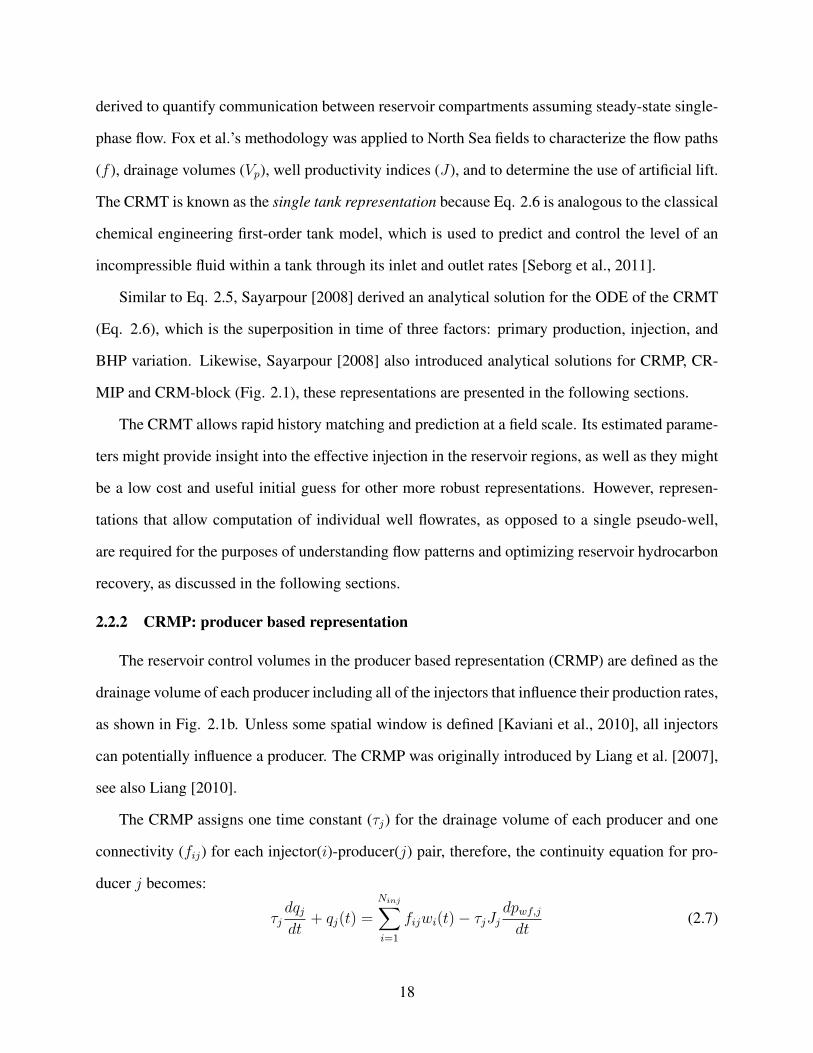
derived to quantify communication between reservoir compartments assuming steady-state single-

phase flow. Fox et al.’s methodology was applied to North Sea fields to characterize the flow paths

(f ), drainage volumes (Vp), well productivity indices (J), and to determine the use of artificial lift.

The CRMT is known as the single tank representation because Eq. 2.6 is analogous to the classical

chemical engineering first-order tank model, which is used to predict and control the level of an

incompressible fluid within a tank through its inlet and outlet rates [Seborg et al., 2011].

Similar to Eq. 2.5, Sayarpour [2008] derived an analytical solution for the ODE of the CRMT

(Eq. 2.6), which is the superposition in time of three factors: primary production, injection, and

BHP variation. Likewise, Sayarpour [2008] also introduced analytical solutions for CRMP, CR-

MIP and CRM-block (Fig. 2.1), these representations are presented in the following sections.

The CRMT allows rapid history matching and prediction at a field scale. Its estimated parame-

ters might provide insight into the effective injection in the reservoir regions, as well as they might

be a low cost and useful initial guess for other more robust representations. However, represen-

tations that allow computation of individual well flowrates, as opposed to a single pseudo-well,

are required for the purposes of understanding flow patterns and optimizing reservoir hydrocarbon

recovery, as discussed in the following sections.

2.2.2 CRMP: producer based representation

The reservoir control volumes in the producer based representation (CRMP) are defined as the

drainage volume of each producer including all of the injectors that influence their production rates,

as shown in Fig. 2.1b. Unless some spatial window is defined [Kaviani et al., 2010], all injectors

can potentially influence a producer. The CRMP was originally introduced by Liang et al. [2007],

see also Liang [2010].

The CRMP assigns one time constant (τj) for the drainage volume of each producer and one

connectivity (fij) for each injector(i)-producer(j) pair, therefore, the continuity equation for pro-

ducer j becomes:

τjdqjdt

+ qj(t) =

Ninj∑i=1

fijwi(t)− τjJjdpwf,jdt

(2.7)

18

In Eq. 2.7, the main difference from Eq. 2.3 is the first term on the right side, which is the

total injected rate from the Ninj injectors that affect producer j. Since only one time constant

is assigned for each producer, the CRMP assumes that the production rate will respond with the

same time constant to changes in wi(t) for all of the Ninj injectors, but with different gains (fij).

For this reason, the CRMP is not recommended for very heterogeneous reservoirs, working better

when near-homogeneity is present close to the producers and all injectors are at similar distances

from the producer, such as for a patterned waterflood.

2.2.3 CRMIP: injector-producer pair based representation

The injector-producer pair based representation (CRMIP) assigns one time constant (τij) and

one connectivity (fij) for each injector(i)-producer(j) pair, as shown in Fig. 2.1c, mitigating the

problem mentioned above but increasing the number of parameters. This model was first proposed

by Yousef et al. [2006], and the continuity equation for each control volume is similar to Eq. 2.3:

τijdqijdt

+ qij(t) = fijwi(t)− τijJijdpwf,jdt

(2.8)

where qij is the production rate in producer j from the injector(i)-producer(j) pair control volume,

as well as Jij is the productivity index associated with such a control volume. Then, superposition

in space is applied to obtain the total production rate of each producer, i.e. the contributions from

all of the injectors are summed up:

qj(t) =

Ninj∑i=1

qij(t) (2.9)

There are some significant differences between the analytical solutions of Sayarpour et al.

[2009b] and the one originally presented by Yousef et al. [2006]. The use of Sayarpour et al.’s

solution is recommended in cases where it is not desired to restrict the primary depletion and BHP

term to an exponential decline, but to a sum of exponential terms at the expense of estimating more

productivity indices.

19

2.2.4 CRM-block: blocks in series representation

The first-order tank formulation assumes immediate response to variations in the injection rates.

In order to overcome this limitation, Sayarpour (2008, Sec. 3.5) extended the CRMT and CRMIP

to consider the time delay in the producers response. Hence, the injector-producer control volume

was divided in several blocks, as a tanks in series model (Fig. 2.1d). This representation was called

CRM-block and is recommended for cases with high dissipation, such as low permeability, high

frequency injection signal, and/or distant injector-producer pairs.

Sayarpour (2008, Sec. 3.5) derived the following analytical solution for the CRMT-block for

the case of a single step change in the injection rate and constant producer’s BHP:

q(t) = qB(t0)e−(t−t0)τB +

B−1∑b=1

(qb(t0)e

−(t−t0)τb

B−b∏a=1

(1− e−(t−t0)τa )

)+ w(t)

B∏b=1

(1− e−(t−t0)

τb ) (2.10)

where B is the total number of blocks between the pseudo-injector and pseudo-producer. This

solution was extended to the CRMIP-block representation including the interwell connectivities in

the injection term, accounting for the number of blocks between each injector-producer pair (Bij),

and summing the production rates of the control volumes associated to a producer:

qj(t) =

Ninj∑i=1

qij(t) =

Ninj∑i=1

qijBij(t0)e−(t−t0)τijBij +

+

Ninj∑i=1

Bij−1∑b=1

qijb(t0)e−(t−t0)τijb

Bij−b∏a=1

(1− e−(t−t0)τija )

+

Ninj∑i=1

fijwi(t)

Bij∏b=1

(1− e−(t−t0)τijb ) (2.11)

Holanda (2015, Sec. 3.2.4) derived the transfer function for the CRMIP-block representa-

tion accounting for variable producers’ BHP. This approach enables the application of these mod-

els in cases of multiple variations in the injection rates and producers’ BHP without requiring

long analytical derivations from higher-order linear ODE’s. An alternative approach presented by

Sayyafzadeh et al. [2011] is to introduce a time lag in a first-order transfer function (single-tank)

instead of using higher-order transfer functions (tanks in series).

20

Although the CRM-block representation is important from a conceptual point of view, show-

ing that it is always possible to increase model complexity, this model has only been applied in

a few studies [Kabir and Lake, 2011, Li et al., 2017]. This indicates that, in general, it is not an

attractive solution in the pursuit of a simplified reservoir model. One practical issue is the signif-

icant increase in the number of parameters. To mitigate this problem, Sayarpour [2008] suggests

to consider an equal time constant (τb) for all blocks and adjust the number of blocks (B) in the

history matching. However, this approach generates another issue because many history matching

problems have to be solved to select the most appropriate model. Additionally, pressures and rates

of the blocks cannot be attributed to particular reservoir regions, as these control volumes are not

spatially defined. In other words, the CRM-block concept is set mainly to mimic the lag in the

production response.

2.2.5 Multilayer CRM: blocks in parallel representation

It is common to have impermeable layers interbedded in the reservoir rock, hence modeling

the fluid flow to the wells in a compartmentalized manner is more realistic than assuming a single

layer, as in the previous representations. Furthermore, production logging tools (PLT) enable

detection of the fraction of the total flow coming from each compartment for each producer, i.e.

for the α-th layer, qjα = fPLT,jαqj . On the other hand, the injection rate distribution profile for

such compartments usually are not inferred, which is a critical control for hydrocarbon recovery

optimization. Based on these facts, Mamghaderi et al. [2012] proposed a multilayer CRM (or ML-

CRM, Fig. 2.1e), which couples PLT data with the CRMP to infer the injected fluid allocation to

each layer. In this case, it is necessary to define two levels of allocation factors: 1) f ′iα represents

the fraction of injected fluid from injector i allocated to layer α; 2) fijα represents the fraction of

f ′iαwi allocated to producer j.

In contrast to Mamghaderi et al. [2012], Moreno [2013] generated a ML-CRMP representa-

tion assuming that the injection profile (f ′iα’s) is known and the production in each layer is un-

known. This is plausible in the case of smart injection wells, but no smart production or PLT data

(fPLT,jα’s) are available. Moreno [2013] presented two formulations for the ML-CRMP: 1) assign-

21

ing different τjα’s for the layers, i.e. each producer has one time constant per layer; 2) assigning

a single time constant (τj) for each producer, resulting in a significant reduction in the number of

parameters. Although it is reasonable to expect different time constants for the layers due to their

distinct properties, Moreno’s case study suggested that, in mature fields, both approaches provide

similar accuracy because the reservoir fluids are nearly incompressible. Additionally, the produc-

tion response is more sensitive to variations in fijα’s than in τjα’s [Jafroodi and Zhang, 2011,

Kaviani et al., 2014, Holanda et al., 2018d]. Therefore, in many cases, the second approach may

be a valid strategy to reduce the number of parameters for the history matching.

As presented in the model of Mamghaderi and Pourafshary [2013], the complexity of the ML-

CRM increases significantly when reservoir layers are not separated by completely sealing rocks,

but in hydraulic communication, resulting in cross-flow between the control volumes. Zhang et al.

[2015] complemented the previous models by considering also the case of known injection and

production per layer and varying producers’ BHP.

The ML-CRM’s previously mentioned extended the CRMP material balance (Eq. 2.7) to each

layer (α), such that these models can be summarized as follows:

τjαdqp,jαdt

+ qp,jα(t) =

Ninj∑i=1

f ′iαfijαwi(t)− τjαJjαdpwf,jdt

(2.12)

where qp,jα is the total production rate contributed from layer α disregarding the crossflow (Qc,jα,

contribution from other layers), and is related to the observed total production rate in layer α

(fPLT,jαqj(t)) by:

qp,jα(t) = fPLT,jαqj(t)−Qc,jα(t) (2.13)

The following constraints are necessary for mass conservation:

L∑α=1

f ′iα = 1 (2.14)

22

L∑α=1

fPLT,jα = 1 (2.15)

L∑α=1

Qc,jα(t) = 0 (2.16)

Equation 2.16 was introduced by Zhang et al. [2015] to take into account that the crossflow

fluid leaving a layer (Qc,jα(t) < 0) must be entering another (Qc,jα(t) > 0).

Although Mamghaderi and Pourafshary [2013] and Zhang et al. [2015] presented formulations

that contemplate the cases of crossflow between layers, one must be careful while increasing model

complexity. As the number of parameters increase, there will be more combinations that satisfac-

torily fit the history matched data, and the risk of many of these models providing a poor forecast

also increases. Also, the progression of crossflow terms in time may not be properly captured by

this approach.

In addition to the previously mentioned references, recent developments and applications of

ML-CRM’s can be found in Fraguío et al. [2017], Gamarra et al. [2017], Zhang et al. [2017], and

Prakasa et al. [2017].

2.3 CRM parameters physical meaning

2.3.1 Connectivities

The interwell connectivity, fij , also known as gain or allocation factor, is defined by the volume

fraction of injected fluid from injector i that can be attributed to the production at well j. Therefore,

at stabilized flow conditions, an increase in the injection rate by ∆wi corresponds to an increase

in the total production rate by ∆qj = fij∆wi in reservoir volumes (Fig. 2.2a). This information

is essential for improved management in secondary and tertiary recovery processes, providing an

understanding of the reservoir behavior and response to control variables.

Albertoni and Lake [2003] inferred interwell connectivities in the cases of balanced and un-

balanced waterflooding by correlating injection and production rate fluctuations via a multivariate

linear regression (MLR) model. They used diffusivity filters to account for the time lag in the

23

Dimensionless Time

3tD =

t

=

40 2 4 6 8 10 12 14 16 18

Norm

alizedProductionRate

0

0.5

1

1.5

2

2.5

3a) Succession of Step Changes in Injection Rate

f=0.25

f=0.5

f=0.75

f=1.0

injection

Dimensionless Time

3tD =

t

=

4-1 0 1 2 3 4 5

"q D

="

q(t)

f"

w

0

0.63

0.860.951

b) Type Curve for Unit Step Injection

production "qD

injection

Figure 2.2: (a) CRM response to a sequence of step injection signals for several values of interwellconnectivity. (b) Physical meaning of time constants: percent of stationary response achieved at aspecific dimensionless time.

production response. The MLR model was a precursor for the CRM presented by Yousef et al.

[2006]. Analogously to the Albertoni and Lake [2003] model, Dinh and Tiab [2008] used only

BHP fluctuation data to estimate interwell connectivities via MLR, without requiring diffusivity

filters.

Gentil [2005] interpreted the regression coefficients (interwell connectivities) of the MLR

model for patterned waterfloods as the ratio of the average transmissibility (Tij) between injec-

24

tor (i) and producer (j) to the sum of the transmissibilities between injector (i) and all producers:

fij =Tij∑Nprod

j=1 Tij(2.17)

Even though such physical meaning has been extended to the gains (fij) in the CRM literature,

one must be aware that it is applicable to patterned mature waterfloods when the injection rates and

producer’s BHP are approximately constant and there are no significant changes in the flow pattern,

which is a very restrictive condition. Also, the injector-producer transmissibilities (Tij’s) have not

been quantified, and Eq. 2.17 has been used more to guide a qualitative interpretation. Since

the interwell connectivity is defined as a fraction of the flowrates, a more consistent theoretical

equation is proposed here:

fij =Tij∆pij∑Nprod

j=1 Tij∆pij(2.18)

The following material balance constraint is a consequence of the physical meaning of the

interwell connectivities:

Nprod∑j=1

fij ≤ 1 (2.19)

where the summation above is less than unity if fluid is being lost to a thief zone, and equal to unity

otherwise. Injected fluid might also be lost due to water flowing to the region below the WOC, to

an aquifer, to underpressured reservoir layers, or even to other communicating reservoirs, resulting

in inefficient injection.

Regarding the dynamic behavior of fij’s, they tend to be approximately constant after water

breakthrough, unless there are major perturbations to the streamlines, such as shut-in wells and

large variations in injection rates and producer BHP’s. This point is exemplified by Jafroodi and

Zhang [2011] for a regular waterflooding and Soroush et al. [2014] for a heavy oil waterflood-

ing cases. Such observation can also be extended to the τij’s and Jij’s. Therefore, after water

25

breakthrough, the parameters in the CRM governing ODE’s (Eqs. 2.6-2.8 and 2.12) are frequently

considered constant, resulting in a linear ODE.

One of the assumptions in the CRM’s previously presented is that there is a constant average-

reservoir fluid density that represents the system. This is valid in a mature waterflooding because

water is slightly compressible and there are slight changes in the saturation. However, before

water breakthrough, this assumption is less likely to be valid due to the sharp change in sat-

uration in the water front and significantly higher compressibility of the oil phase. Izgec and

Kabir [2010a] extended the CRM’s applicability to prebreakthrough conditions by incorporating a

pressure-dependent fluid density function to Eq. 2.1, obtaining:

ctVpdp

dt=ρw,inρw

w(t)− ρo,outρo

qo(t) (2.20)

where ρw and ρo are the average densities of water and oil in the control volumes, respectively,

ρw,in is the input water density, ρo,out is the output oil density and qo(t) is the oil production rate

(res bbl/day). Since water is slightly compressible, it is plausible to assume ρw,inρw

= 1.

Izgec and Kabir’s (2010a) approach enables one to gain connectivity information during the

early stage of a flooding process. In this sense, CRM serves as a diagnostic tool that allows

remedial actions regarding injected fluids’ allocation, avoiding early breakthrough and reducing

volumes lost to thief zones, as well as providing a clue for future well placements.

2.3.1.1 Aquifer-producer connectivity

If there is an aquifer providing extra pressure support to the reservoir, the best approach is

to couple CRM with an aquifer model in order to account for the controllable (injection rates)

and uncontrollable (aquifer) influxes separately. Izgec and Kabir [2010b] applied the Carter-Tracy

aquifer model to estimate the instantaneous water influx and added it to the allocated injection in

the CRMP equation (∑Ninj

i=1 fijwi(t) + waj , in Eq. 2.7). Their approach accounts for nonuniform

support to the producers by attaching a different aquifer model to each producer, resulting in a large

increase in the number of parameters (3 per aquifer). The strategy adopted to reduce the number

26

of parameters is to define certain regions with common porosity, permeability and thickness, while

the drainage radii are computed individually for each producer. Izgec [2012] proposed a simplified

CRM-aquifer approach assuming a single aquifer connected to a tank. First, the CRMT is coupled

with the Carter-Tracy aquifer model to estimate the field instantaneous water influx. Second, the

CRMIP is coupled with the single aquifer model and aquifer-producer connectivities (faj) are

established to account for the additional influx (fajwaj). The cases of early injection pose an

additional difficulty to characterize the aquifer, since the scenarios of high volumes lost to thief

zones with large aquifer or low volumes lost to thief zones with small aquifer might both honor

the material balance. Izgec [2012] suggests generating equiprobable realizations to mitigate this

problem.

2.3.1.2 Connectivity interpretation within a flood management perspective

The field studies developed by Parekh and Kabir [2013] are useful to illustrate the concepts

of interwell and inter-reservoir connectivities and their application to reservoir management. The

CRM derived fij’s corroborated tracer testing results. The understanding gained from reservoir

connectivity can often be tied to the geological characteristics which control hydrocarbon recovery.

For example, high permeability pathways, such as fractures, can cause a rapid water breakthrough

in a producer (high fij) or water leaking to a thief zone (low fij), and both cases are associated

with poor sweep-efficiency, requiring redesign of the flooding process (e.g. choose a more efficient

EOR fluid). Parekh and Kabir [2013] also suggest a methodology to analyze thief zones applying

WOR plot, modified-Hall plot, 4D seismic, rate transient analysis and the CRM.

Thiele and Batycky [2006] defined injection efficiency as the volume ratio of incremental oil

obtained by fluid injected. Their empirical management approach consists in assigning gradually

increasing flowrates to more efficient injectors and reducing it to the less efficient ones based on

an established equation. This is applied sequentially, updating injection efficiencies and allocation

factors every time step via streamlines simulation. Instead of using numerical optimization, their

method exemplifies how streamline allocation factors and water-cut information can improve wa-

terflooding management solely by simple reservoir engineering judgments. As it will be discussed

27

in Section 2.5, fij’s can be updated sequentially via ensemble Kalman filters, this allows the use

of Thiele and Batycky’s (2006) method with the CRM.

2.3.2 Time constants

The CRM time constant, previously defined in Eq. 2.4, accounts for dissipation of the input

signals in the porous media; these input signals are injection rates and producer BHP’s which are

varying in time. As previously mentioned, τ is also related to the production decline during primary

recovery. In fact, τ ’s are intrinsically associated with pressure diffusion, while time of flight in

streamlines simulation is associated with the evolving saturation of the phases. If a step increase

is applied to injection rates in the CRMT, CRMP, CRMIP or ML-CRM (first order systems), one

time constant (t = τ ) is the time to achieve 63.2% of the final production rate; 95.0% is achieved

at t = 3τ (Fig. 2.2b).

A straightforward analysis of Eq. 2.4 shows that a large pore volume (Vp ↑), a very compress-

ible system (ct ↑) and/or a low productivity index (J ↓) results in a large τ , and therefore large

dissipation of the input signals and slow decline of the primary production term. In contrast, a

fast transmission of the input signals and fast decline of the primary production term results from

small τ , which is obtained in the cases of small pore volume (Vp ↓), low total compressibility (ct ↓)

and/or high productivity index (J ↑).

For an overview on the physical meaning of productivity indices and models, the reader is

referred to Economides et al. [2013].

2.4 CRM for primary production

As presented in the works of Nguyen et al. [2011] and Izgec and Kabir [2012], the continuity

equation (Eq. 2.3) is simplified in the case of primary production by assigning w(t) = 0. The

formulations presented in these works permit quantification of the drainage pore volumes (Vpj , if ct

is known) and productivity indices (Jj) of each producer, as well as average compartment pressure

(p(t), from Eq. 2.2) only from the primary production decline and BHP fluctuations. These simple

methods are an alternative to the traditional build-up test with the advantage that no shut-in time

28

is required, therefore production is not delayed, and can be easily applied to multiwell systems

without requiring prior knowledge of the reservoir properties (such as porosity, permeability and

thickness). Izgec and Kabir [2012] extended the application of this method to gas wells by using

pseudopressure functions.

Nguyen et al. [2011] applied the CRM integrated form (ICRM, to be discussed in Section 2.5)

in a sequential manner (piecewise time windows) to identify the increasing drainage volume during

transient flow until the onset of pseudosteady-state (PSS), when Vpj tends to be constant, as well

as a reduction in Vpj due to infill drilling. Varying BHP’s of neighboring wells and workovers also

change the no flow boundaries and consequently Vpj’s. Izgec and Kabir [2012] used longer time

windows, suggesting to use only PSS data, and validated the drainage volume results with the ones

obtained via streamlines simulation. Also, Izgec and Kabir [2012] qualitatively inferred interwell

connectivity and reservoir compartmentalization by analyzing Vpj’s before and after drilling new

wells.

The evolving behavior of Vpj’s and pressure depletion during primary production are valuable

information for reservoir management that can be obtained via these methods. However, neither

study provided a robust model capable of predicting the time-varying behavior of Vpj , which could

lead to a more effective BHP control, for example; this should be the subject of future research.

2.5 CRM history matching

Capacitance Resistance Models are generated through history matching, where the model pa-

rameters are adjusted so that the total flowrates predicted by CRM “fit” the observed production

history. This is essentially an optimization problem where many types of objective function can be

chosen to penalize the mismatches; the following least squares function is a common choice:

min zobj = min(qpred − qobs)TCe

−1(qpred − qobs) (2.21)

where qpred and qobs ∈ <NtNprod×1 and are the vectors of predicted and observed, respectively,

total fluid rates for all of the wells and at every time step; Ce ∈ <NtNprod×NtNprod and is the

29

covariance matrix of the measurement and modeling errors; Nt is the number of time steps. qpred

is computed from the solution of the CRM representation (e.g. Eq. 2.5).

While history matching data, it is necessary to restrict the solution space to physically plausible

values of the parameters. Therefore, Eq. 2.21 is subject to several constraints:

minΨ

zobj(Ψ) such that

a ·Ψ ≤ b

aeq ·Ψ = beq

lb ≤ Ψ ≤ ub

(2.22)

where Ψ is the vector of parameters (e.g. f , τ and J); zobj(Ψ) is the objective function (scalar,

Eq. 2.21); a and aeq are matrices, b and beq are vectors for the inequality and equality linear

constraints, respectively; and lb and ub are lower and upper bounds of the parameters, respectively.

Holanda [2015] and Holanda et al. [2015] present the structure of these matrices for the CRMT,

CRMP and CRMIP representations. Equation 2.19 is an inequality constraint that is valid for all

representations, Eq. 2.9 is an equality constraint for the CRMIP and Eqs. 2.14, 2.15 and 2.16 are

equality constraints for the ML-CRM.

There are several optimization algorithms capable of solving the problem stated by Eqs. 2.21

and 2.22. It is beyond the scope of this dissertation to discuss the mathematical formulation as well

as the advantages and disadvantages of each. Instead the reader is referred to a comprehensive

literature review on reservoir history matching by Oliver and Chen [2011]. For reference, Tab.

2.1 briefly highlights some aspects of several algorithms and their application to CRM history

matching.

Probabilistic history matching allows obtaining multiple CRM realizations to analyze the un-

certainty in the parameter estimates and production forecast. For this purpose, Kaviani et al. [2014]

used the bootstrap, which is a sampling with replacement method. Sayarpour et al. [2011] history

matched multiple realizations of CRM with a Buckley-Leverett-based fractional flow model (Sec.

2.7) starting from different initial guesses. Their main objective was to assess the uncertainty in

reservoir parameters such as porosity, irreducible-water and residual-oil saturations.

30

Table 2.1: Some of the optimization algorithms used for CRM history matching.

Reference Algorithm Highlights

Kang et al. [2014] Gradient projection

method within a

Bayesian inversion

framework.

Converted Eq. 2.19 into a equality constraint.

Analytical formulation for gradient compu-

tation based on sensitivity of the model re-

sponse to its parameters. Each iteration takes

the direction of the projected gradient that sat-

isfies the constraints.

Holanda et al.

[2015]

Sequential quadratic pro-

gramming (SQP), numer-

ical gradient computa-

tion, BFGS approxima-

tion for the Hessian ma-

trix.

Even though gradient-based formulations

may be fast and straightforward to implement,

they also rely on a proper choice of initial

guess to avoid convergence to a local minima.

Weber [2009]

and Lasdon et al.

[2017]

GAMS/CONOPT

(gradient-based, lo-

cal search), automatic

computation of first and

second partial deriva-

tives.

The objective function is based on the mis-

match for a one step ahead prediction from

the measured data. The problem is solved in

a sequence of four steps that include defining

a suitable initial guess, determining injector-

producer pairs with zero gains and excluding

outliers. A global optimization algorithm ca-

pable of identifying local minima has demon-

strated the occurrence of multiple local solu-

tions in several examples.

31

Table 2.1: Some of the optimization algorithms used for CRM history matching (continued).

Reference Algorithm Highlights

Wang et al. [2017] Stochastic simplex

approximate gradient

(StoSAG).

For an example of a heterogenoues reservoir

with 5 injectors and 4 producers, the StoSAG

demonstrated convergence with less iterations

and to a smaller value of objective function

than with the projected gradient and ensemble

Kalman filter methods.

Mamghaderi

et al. [2012]

and Mamghaderi

and Pourafshary

[2013]

Genetic algorithms

(global optimization)

Genetic algorithm is applied for the history

matching of the ML-CRM and justified by the

significant increase in the number of parame-

ters compared to other CRM representations

(Tab. 2.2).

Jafroodi and

Zhang [2011] and

Zhang et al. [2015]

Ensemble Kalman filter

(EnKF).

Model parameters are sequentially updated as

more data is gathered. So, it is possible to

track and analyze the time-varying behavior

of the parameters. Multiple models are ob-

tained providing insight in the uncertainty of

production forecasts and estimated parame-

ters. Model constraints have not been explic-

itly considered.

2.5.1 Dimensionality reduction

Table 2.2 shows the number of parameters to be estimated for each CRM representation. As

the number of parameters increase, issues with the non-uniqueness of the history matching solu-

32

tion become more concerning, so it is important to gather more data (e.g. tracer and interference

tests, PLT and smart completions data for the multilayer reservoirs) and/or measure at a higher fre-

quency to reduce ambiguities. It is also highly recommended to consider dimensionality reduction

techniques, which can reduce the impact of spurious correlations within the production data in the

model fitting. The following are examples of such techniques:

Table 2.2: Dimension of the history matching problem for several CRM representations withoutdimensionality reduction. * The number of parameters for the ML-CRM was estimated based onEqs. 2.12-2.13, assuming no data available from production logging tools or smart completions(i.e. unknown fPLT,jα and f ′iα ) and occurrence of crossflow between layers.

ModelDimension

Constant BHP Varying BHPCRMT 2 3

CRMP (Ninj + 1)Nprod (Ninj + 2)Nprod

CRMIP 3NinjNprod 4NinjNprod

CRMT-Block B + 1 B + 2

CRMIP-Block (B + 2)NinjNprod (B + 3)NinjNprod

ML-CRM* NL(Nprod(Ninj +Nt + 2) +Ninj) NL(Nprod(Ninj +Nt + 3) +Ninj)

• Define a spatial window of active injector-producer pairs based on the interwell distance and

reservoir heterogeneity, fij = 0 for wells outside the spatial window [Kaviani et al., 2010];

• Define a maximum number of nearest injectors that could affect a producer well [Lasdon

et al., 2017];

• Assign the same τj to all layers in the ML-CRM [Moreno, 2013];

• Instead of applying the CRM-block representation, i.e. blocks in series, use a first-order tank

with a time delay [Sayyafzadeh et al., 2011];

• Assign a single productivity index per producer in the CRMIP representation [Altaheini

et al., 2016].

33

2.5.2 Alternative CRM formulations

Besides defining which optimization algorithm and dimensionality reduction technique are

suitable for application, it is also important to be aware of alternative CRM formulations that

may facilitate the history matching under specific circumstances.

2.5.2.1 Matching cumulative production: the integrated capacitance resistance model (ICRM)

The integrated capacitance resistance model (ICRM) is based on the same control volume as

the CRMP, however the ODE is integrated providing a linear model for cumulative production

[Kim, 2011, Nguyen et al., 2011, Kim et al., 2012]:

Np,jk = (qj0 − qjk)τj +

Ninj∑i=1

(fijWik) + Jjτj(pwf,j0 − pwf,jk) (2.23)

where Np,jk is the cumulative total liquid production of producer j at end of the k-th time step

(tk), and Wik is the cumulative volume of water injected in injector i at tk. In this case, the history

matching is performed for the cumulative total liquid production. The advantage of curve fitting

a linear model is that there is a unique solution which is obtained in a finite number of iterations,

so it is computationally very fast, and it is easier to determine confidence intervals for the param-

eters. On the other hand, the cumulative production is smoother than rates and always increases

with time, so mismatches in the last data points of the production history may be penalized more

than the early ones and overfitting may be an issue. To mitigate these problems, Holanda et al.

[2018d] proposed a normalization of the ICRM history matching objective functions based on the

propagation of error of individual rates in the cumulative production; the results presented for two

reservoirs showed better agreement with the connectivity estimates from CRMP and CRMIP.

Laochamroonvorapongse et al. [2014] suggests that even if the nonlinear models are applied,

an improvement in the quality of the history matching solution is obtained by first matching CRM

production rates, then using the solution as an initial guess for the matching of CRM cumulative

production. Another approach to determining initial guesses is to use the gains calculated from the

case of a homogeneous reservoir, as described by Kaviani and Jensen [2010].

34

2.5.2.2 Unmeasured BHP variations: segmented CRM

Situations where producers’ BHP data are not available or not measured with the appropriate

frequency are common. In these cases, the assumption of constant BHP may not be plausible,

so it is important to account for BHP variations while history matching models even if they are

unmeasured. The segmented CRM [Kaviani et al., 2012, Kaviani, 2009] is a model proposed for

the detection and quantification of the effects of such unmeasured BHP variations:

qj(tn) = qj(t0)e− tn−t0

τpj +

Ninj∑i=1

n∑k=1

fije− tn−tk

τij (1− e−∆tkτij )wi(tk) + qBHPj(Ts) (2.24)

where qBHPj(Ts) is a constant added to the analytical solution that accounts for the unknown BHP

variations in the segmented time Ts and is a parameter included in the history matching. Kaviani

et al. [2012] proposed an algorithm for the identification of the segmentation times, i.e. when the

producer BHP changes significantly.

2.5.2.3 Changes in well status: compensated CRM

A common assumption of most CRM representations is a constant number of active producers;

however well status changes may occur frequently in the field (flowing, shut-in, and conversions

from producer to injector). Therefore, specific strategies must be pursued for history matching in

these cases to avoid redefining a time window and reestimating all of the parameters every time

there is a change in well status. Significant changes in flow patterns and allocation of injected fluids

are expected as wells are shut or opened. The compensated CRM [Kaviani et al., 2012, Kaviani,

2009] uses the superposition principle to treat shut-in producers as a combination of two wells: the

actual producer with open status and a virtual injector that re-injects all of the produced fluid at the

same location. Considering constant producers’ BHP, the analytical solution for the compensated

CRM is:

qjν(tn) = qj(t0)e− tn−t0

τpj +

Ninj∑i=1

n∑k=1

fijνe− tn−tk

τijν (1− e−∆tkτijν )wi(tk) (2.25)

35

where the subscript ν indicates that the ν-th producer is shut-in. In this case, the interwell connec-

tivities are redefined as:

fijν = fij + λνjfiν (2.26)

where λνj is the interwell connectivity between the virtual injector equivalent to the ν-th producer.

In other words, the λνj also measures the producer-producer connectivity observed by the change

at well j when well ν is shut-in. So, λνj’s and τijν’s are additional parameters estimated during

the history matching. As mentioned by the authors, this model is also useful when producers are

converted to injectors.

2.6 CRM sensitivity to data quality and uncertainty analysis

As studied by Tafti et al. [2013], the identification of the CRM parameters and their underlying

uncertainty are intrinsically related to:

• the amplitude and frequency of uncorrelated variations in the input signals (injection rates

and producers’ BHP), because the most relevant dynamic aspects of the system must be

observed in the output signals (production rates);

• the amount of data available for history matching, i.e. sampling frequency (e.g. whether

production data are reported daily or monthly) and length of the history matching window;

• the properties of the reservoir system, such as permeability distribution, fluid saturation and

total compressibility.

Originally, the CRM was developed as a dynamic reservoir model with interwell connectivities

estimated from variations in the production and injection data that commonly occur in field opera-

tions. So, ideally, it would not be necessary to change injection rates or producers’ BHP merely for

the identification of the CRM parameters. However, if in any circumstances it is desired to improve

the information content of the input/output signals, the studies of Tafti et al. [2013] and Moreno

and Lake [2014b] provide guidelines based on systems identification theory. The approach devel-

oped by Tafti et al. [2013] relies on previous information of the systems dynamics, which might be

36

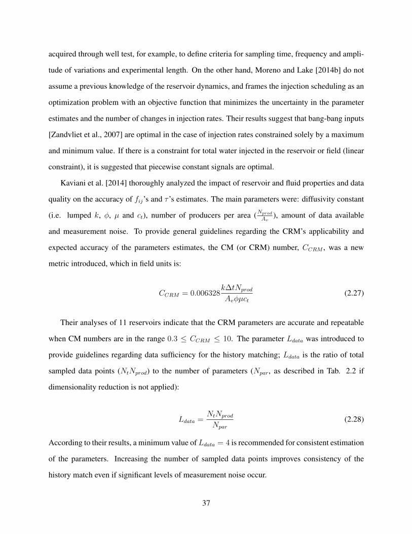
acquired through well test, for example, to define criteria for sampling time, frequency and ampli-

tude of variations and experimental length. On the other hand, Moreno and Lake [2014b] do not

assume a previous knowledge of the reservoir dynamics, and frames the injection scheduling as an

optimization problem with an objective function that minimizes the uncertainty in the parameter

estimates and the number of changes in injection rates. Their results suggest that bang-bang inputs

[Zandvliet et al., 2007] are optimal in the case of injection rates constrained solely by a maximum

and minimum value. If there is a constraint for total water injected in the reservoir or field (linear

constraint), it is suggested that piecewise constant signals are optimal.

Kaviani et al. [2014] thoroughly analyzed the impact of reservoir and fluid properties and data

quality on the accuracy of fij’s and τ ’s estimates. The main parameters were: diffusivity constant

(i.e. lumped k, φ, µ and ct), number of producers per area (NprodAv

), amount of data available

and measurement noise. To provide general guidelines regarding the CRM’s applicability and

expected accuracy of the parameters estimates, the CM (or CRM) number, CCRM , was a new

metric introduced, which in field units is:

CCRM = 0.006328k∆tNprod

Avφµct(2.27)

Their analyses of 11 reservoirs indicate that the CRM parameters are accurate and repeatable

when CM numbers are in the range 0.3 ≤ CCRM ≤ 10. The parameter Ldata was introduced to

provide guidelines regarding data sufficiency for the history matching; Ldata is the ratio of total

sampled data points (NtNprod) to the number of parameters (Npar, as described in Tab. 2.2 if

dimensionality reduction is not applied):

Ldata =NtNprod

Npar

(2.28)

According to their results, a minimum value ofLdata = 4 is recommended for consistent estimation

of the parameters. Increasing the number of sampled data points improves consistency of the

history match even if significant levels of measurement noise occur.

37

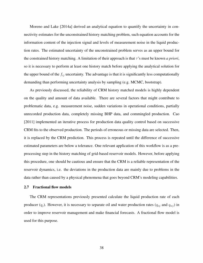
Moreno and Lake [2014a] derived an analytical equation to quantify the uncertainty in con-

nectivity estimates for the unconstrained history matching problem, such equation accounts for the

information content of the injection signal and levels of measurement noise in the liquid produc-

tion rates. The estimated uncertainty of the unconstrained problem serves as an upper bound for

the constrained history matching. A limitation of their approach is that τ ’s must be known a priori,

so it is necessary to perform at least one history match before applying the analytical solution for

the upper bound of the fij uncertainty. The advantage is that it is significantly less computationally

demanding than performing uncertainty analysis by sampling (e.g. MCMC, bootstrap).

As previously discussed, the reliability of CRM history matched models is highly dependent

on the quality and amount of data available. There are several factors that might contribute to

problematic data, e.g. measurement noise, sudden variations in operational conditions, partially

unrecorded production data, completely missing BHP data, and commingled production. Cao

[2011] implemented an iterative process for production data quality control based on successive

CRM fits to the observed production. The periods of erroneous or missing data are selected. Then,

it is replaced by the CRM prediction. This process is repeated until the difference of successive

estimated parameters are below a tolerance. One relevant application of this workflow is as a pre-

processing step in the history matching of grid-based reservoir models. However, before applying

this procedure, one should be cautious and ensure that the CRM is a reliable representation of the

reservoir dynamics, i.e. the deviations in the production data are mainly due to problems in the

data rather than caused by a physical phenomena that goes beyond CRM’s modeling capabilities.

2.7 Fractional flow models

The CRM representations previously presented calculate the liquid production rate of each

producer (qj). However, it is necessary to separate oil and water production rates (qoj and qwj) in

order to improve reservoir management and make financial forecasts. A fractional flow model is

used for this purpose.

38

2.7.1 Buckley-Leverett adapted to CRM

The Buckley and Leverett [1942] physics-based model is probably the most popular amongst

reservoir engineers. It assumes linear horizontal flow of immiscible and incompressible phases in

a 1D homogeneous reservoir, and neglects capillary pressure and gravitational forces. It allows

estimation of the location of the flood-front, saturation profile and water-cut at the producer, given

the relative permeability curves and fluid viscosities (Figs. 2.3a-b). Sayarpour [2008] presented a

fractional flow model based on the one from Buckley and Leverett [1942] which can be applied

with CRM (see also Sayarpour et al., 2011):

fo(S) = 1−(

1 +(1− S)m

MSn

)−1

(2.29)

where fo is the oil cut (i.e. oil fractional flow at the producer), m and n are relative permeability

exponents from the modified Brooks and Corey [1964] model (Fig. 2.3a), M is the end-point

mobility ratio, and S is the normalized average water saturation, defined as:

S(t) =Sw(t)− Swr

1− Sor − Swr(2.30)

where Swr and Sor are the irreducible water and residual oil saturations, respectively, and Sw(t)

is the saturation at the outlet of the control volume. However, Sayarpour [2008] used the average

water saturation in the control volume, which can be computed through the following material

balance equation:

Sw(tk) = Sw(tk−1) +w∗j (tk)− qwj(tk−1)

Vp∆tk (2.31)

where w∗j (tk) =∑Ninj

i=1 fijwi(tk), which is the effective water injected in the control volume.

Additional calculations are necessary to compute Sw(t) at the outlet of the control volume [Buckley

and Leverett, 1942, Willhite, 1986], the results for a sensitivity analysis in this case are shown in

Fig. 2.3c. This model has six unknowns (m, n, M , Swr, Sor and Vp), so there are many degrees

of freedom. As a result, the parameters of a single history matched model may not correspond to

39

the actual reservoir properties and provide a poor forecast. For this reason, Sayarpour et al. [2011]

used this model mainly for the uncertainty quantification of reservoir parameters (Swr, Sor and φ)

before starting to develop a grid-based reservoir model. An alternative approach to be considered in

the implementation of this fractional flow model is to define m, n, M , Swr, Sor as global reservoir

variables and only a single Vp for each control volume or per producer.

2.7.2 Semi-empirical power-law fractional flow model

Semi-empirical models are an alternative to reduce the number of parameters while applying

a functional form that mimics the observed behavior. For oil cut in an immiscible displacement

process, the function must be monotonically decreasing and with values between 0 and 1. The most

popular fractional flow model for waterflooding in mature fields is the one based on the power-law

relation for water-oil ratio (WOR) derivable from Yortsos et al. [1999], rediscovered by Gentil

[2005], and further developed for CRM by Liang et al. [2007]:

fo(tk) =qoj(tk)

qj(tk)=

1

1 + αjW ∗j (tk)βj

(2.32)

where αj and βj are the fractional flow parameters for producer j, and W ∗j (tk) is the effective

cumulative water injected to the control volumes of producer j up to the k-th time step, defined by:

W ∗j (tk) =

Ninj∑i=1

∫ tk

t0

fijwi(ε)dε ≈Ninj∑i=1

k∑κ=1

fijwi(tκ) (2.33)

In order to ensure physically plausible behavior, both parameters are constrained to being pos-

itive (αj, βj > 0) so that 0 ≤ fo(tk) ≤ 1 and it decreases with W ∗j (tk). Besides the fact that it has

only two parameters, an advantage of this model is that it can be written as a straight line equation

(Fig. 2.4), which facilitates the history matching of oil cut (or oil rates) that can be performed

independently for each producer. Also, the only additional information required after the CRM

history matching are the oil rates.

40

Water Saturation (Sw)0.2 0.4 0.6 0.8

Rela

tive

Perm

eabilit

y(k

r)

0

0.2

0.4

0.6

0.8

1a) Modi-ed Brooks and Corey Model

krw, n = 2, krw;max = 0:15kro, m = 3, kro;max = 0:9

1! SorSwr

krw = krw;maxSn

kro = kro;max(1! S)m

Dimensionless Distance (xD)0 0.2 0.4 0.6 0.8 1

Wate

rSatu

rati

on

(Sw)

0.2

0.3

0.4

0.5

0.6

0.7

0.8b) Flood-Front Advance, 7w = 1:0cp, 7o = 2:0cp

tD = 0:1tD = 0:2tD = 0:3tD = 0:4tD = 0:5tD = 0:6

c) Sensitivity to Parameters

Normalized Time0 1 2

f wj x D

=1

0

0.2

0.4

0.6

0.8

Vp

11.5 22.5 3

tD

0.5 1 1.5 2

f wj x D

=1

0

0.2

0.4

0.6

0.8

Swr

0.050.1630.2750.388 0.5

tD

0.5 1 1.5 2

f wj x D

=1

0

0.2

0.4

0.6

0.8

Sor

0.050.1630.2750.388 0.5

tD

0.5 1 1.5 2

f wj x D

=1

0

0.2

0.4

0.6

0.8

M

0.10.316 1 3.16 10

tD

0.5 1 1.5 2

f wj x D

=1

0

0.2

0.4

0.6

0.8

m

23456

tD

0.5 1 1.5 2

f wj x D

=1

0

0.2

0.4

0.6

0.8

n

23456

Normalized Time0 1 2

f wj x D

=1

0

0.2

0.4

0.6

0.8

Vp

11.5 22.5 3

tD

0.5 1 1.5 2

f wj x D

=1

0

0.2

0.4

0.6

0.8

Swr

0.050.1630.2750.388 0.5

tD

0.5 1 1.5 2

f wj x D

=1

0

0.2

0.4

0.6

0.8

Sor

0.050.1630.2750.388 0.5

tD

0.5 1 1.5 2

f wj x D

=1

0

0.2

0.4

0.6

0.8

M

0.10.316 1 3.16 10

tD

0.5 1 1.5 2

f wj x D

=1

0

0.2

0.4

0.6

0.8

m

23456

tD

0.5 1 1.5 2

f wj x D

=1

0

0.2

0.4

0.6

0.8

n

23456

Normalized Time0 1 2

f wj x D

=1

0

0.2

0.4

0.6

0.8

Vp

11.5 22.5 3

tD

0.5 1 1.5 2

f wj x D

=1

0

0.2

0.4

0.6

0.8

Swr

0.050.1630.2750.388 0.5

tD

0.5 1 1.5 2f w

j x D=

1

0

0.2

0.4

0.6

0.8

Sor

0.050.1630.2750.388 0.5

tD

0.5 1 1.5 2

f wj x D

=1

0

0.2

0.4

0.6

0.8

M

0.10.316 1 3.16 10

tD

0.5 1 1.5 2

f wj x D

=1

0

0.2

0.4

0.6

0.8

m

23456

tD

0.5 1 1.5 2

f wj x D

=1

0

0.2

0.4

0.6

0.8

n

23456

Figure 2.3: (a) Example of modified Brooks and Corey [1964] relative permeability model. (b)Buckley-Leverett prediction of the flood-front advance. (c) Water-cut sensitivity to parameters inEq. 2.29; the title of each subplot indicates which parameter is changing with values shown in thelegends (base case: w = 1 bbl/day, Vp = 1 bbl, Swr = 0.2, Sor = 0.2, M = 0.33, m = 3, n = 2;observation: w and Vp are normalized for the base case).

41

W $j (bbl)

105 106

WO

R

10-2

10-1

100

101a)

PROD3PROD4PROD5PROD7

log(WOR) = log(,j) + -j log(W $j )

W $j

105 106 107

f wj x

D=

1

0.5

0.6

0.7

0.8

0.9

1b)

,j = 1# 10!6

,j = 3:16# 10!7

,j = 1# 10!7

,j = 3:16# 10!8

,j = 1# 10!8

,j = 3:16# 10!9

-j = 1:2

W $j

104 105 106 107

f wj x

D=

1

0.5

0.6

0.7

0.8

0.9

1c)

-j = 1.0-j = 1.2-j = 1.4-j = 1.6-j = 1.8-j = 2.0

,j = 10!7

Figure 2.4: (a) Example of history matching the late time WOR with the power-law relations (thesefour producers are in the reservoir shown in Fig. 2.6a). Water-cut sensitivity to parameters of thesemi-empirical fractional flow model: (b) αj , and (c) βj .

2.7.3 Koval fractional flow model

In contrast to the semi-empirical power-law model that is applicable for mature fields only

(higher values of water cut, e.g. fw ≥ 0.5), the formulation that couples CRM and the Koval

[1963] fractional flow model is more suitable to span the whole life of a waterflooding project, i.e.

0 ≤ fw ≤ 1 [Cao, 2014, Cao et al., 2014, 2015]. The Koval model is physics-based and originally

was formulated for the miscible displacement of solvent in a heterogeneous media, later it was

proven to be equivalent to the Buckley-Leverett model when the relative permeability curves are

straight lines, i.e. m = 1, n = 1 in Eq. 2.29 [Lake, 2014]. The Koval equation for the fractional

flow of water is:

fw =1

1 + 1Kval

(1−SS

) (2.34)

where S is the normalized average water saturation (Eq. 2.30), and Kval is the Koval factor:

Kval = HE (2.35)

42

where H is a heterogeneity factor (H = 1 for homogeneous and H > 1 for heterogeneous porous

media) and E is the effective oil-solvent viscosity ratio:

E =

(0.78 + 0.22

(µoµsv

)0.25)4

(2.36)

Equations 2.34-2.36 set the basis of the Koval model. However, they are expressed in terms of

saturation which is not directly measured in the field, and µo, µsv and H may be unavailable. Cao

[2014] developed the following formulation that is more straightforward for field application when

combined with the CRM:

fw|xD=1

0, tD < 1Kval

Kval−√KvaltD

Kval−1, 1

Kval< tD < Kval

1, tD > Kval

(2.37)

where xD is the dimensionless distance (i.e. distance from injector divided by total distance in the

control volume), fw|xD=1 denotes the water fractional flow at the producer, i.e. the water-cut; tD is

the dimensionless time, which is the cumulative volume injected to the control volume divided by

its total pore volume:

tD =W ∗(t)

Vp(2.38)

where W ∗(t) is given by Eq. 2.33. The reader is referred to Cao et al. (2015, Appendix A) for a

detailed derivation of Eq. 2.37.

Therefore, as in the power-law fractional flow model (Eq. 2.32), there are only two unknowns

per producer in history matching of the Koval model (Vp and Kval). The advantage is that it can

be applied earlier for production optimization in a waterflooding project. Even though the model

includes the prebreakthrough scenario (fw = 0), the parameters cannot be identified before the

water breakthrough. Figure 2.5 shows an application of this model and the water-cut sensitivities to

Vp and Kval. The pore volume (Vp) controls the breakthrough time, shifting the water-cut profile in

43

the semilog plot while Kval defines the shape of the water-cut curve, accounting for heterogeneity

and viscosity ratio. Kval = 1 when µoµw

= 1 and the reservoir is homogeneous (H = 1), as a result

piston-like displacement is observed.

W $j (bbl)

105 106

WO

R

10-2

10-1

100

101a)

PROD3PROD4PROD5PROD7

WOR =Kval !

qKval

tDqKval

tD! 1

W $j (bbl)

104 106 108

f wj x

D=

1

0

0.2

0.4

0.6

0.8

1b)

Vp = 3:2# 104 bblVp = 7:9# 104 bblVp = 2:0# 105 bblVp = 5:0# 105 bblVp = 1:3# 106 bblVp = 3:2# 106 bbl

Kval = 5

W $j (bbl)

104 106 108

f wj x

D=

1

0

0.2

0.4

0.6

0.8

1c)

Kval = 1:0Kval = 2:5Kval = 6:3Kval = 16Kval = 40Kval = 100

Vp = 5# 105 bbl

Figure 2.5: (a) WOR resulting from history matching the early and late time water-cut with theKoval fractional flow model (these four producers are in the reservoir shown in Fig. 2.6a). Water-cut sensitivity to parameters of the Koval fractional flow model: (b) Vp, and (c) Kval.

Cao et al. [2014] presented a fully-coupled formulation for the CRM/Koval fractional flow

model, which accounts for the effects of the evolution of the water front. As saturation changes,

the mobility and total compressibility change accordingly. As a result, the total productivity index

and time constants are a function of the average saturation of the control volumes and present a

significant time-varying behavior at low water cuts. For a review of other fractional flow models,

see Sayarpour [2008].

2.8 CRM enhanced oil recovery

Even though the models presented thus far were mainly developed for waterflooding, the CRM

has also been applied to enhanced oil recovery (EOR) processes. In some reports, the models pre-

viously presented are used exactly in the same way as in waterflooding, while in others specific

developments were carried out to account for the particularities of the EOR process under investi-

gation. This section presents the references and highlights of such developments and applications

44

of the CRM to EOR processes.

In any EOR process, it is critical to understand the displacement efficiency at several scales

(e.g. pore, interwell, basin). Yousef et al. [2009] proposed a flow capacity plot, which serves

as a diagnostic tool for the injection sweep efficiency in the interwell scale. Izgec [2012] also

presented an application of this concept. In this plot, two measures must be computed from the

CRMIP parameters, the cumulative flow capacity (Fmj) and the cumulative storage capacity (Φmj),

which are defined as follows:

Fmj =

∑mi=1 fij∑Ninji=1 fij

(2.39)

Φmj =

∑mi=1 fijτij∑Ninji=1 fijτij

(2.40)

In these summations, the parameters related to producer j are rearranged in decreasing order

of 1τij

, thus i = 1 corresponds to the injector-producer pair with smallest τij and i = Ninj is the

pair with largest τij . Figure 2.6 shows an example of flow capacity plot for four producers in a

channelized reservoir. This plot determines how the flow is distributed across the pore volume

related to each producer, i.e. the percentage of flow coming from a specified percentage of pore

volume. In an ideal displacement, all of the pore volume would be swept evenly. In this case, the

curve would fit the unit slope line. Therefore, the deviations of each curve from the 45o line can

be related to several types of heterogeneity in the porous media (e.g. fractures, high permeability

layers), and serve as a measure of the sweep efficiency of a producer. The closer it is to the 45o

line, the more efficient it is. Therefore, the flow capacity plot allows identification of problematic

wells that may need an EOR process to effectively mobilize the oil left behind the previous flood

front.

The following subsections summarize the CRM references by EOR process and provide some

highlights on the implementation of each work. Even though the complexity of the physical and

chemical interactions between fluids and rock are overlooked by these simple models, generally

45

b)a)

Cumulative Storage Capacity ())0 0.2 0.4 0.6 0.8 1

Cum

ulat

ive

Flo

w C

apac

ity

(F)

0

0.2

0.4

0.6

0.8

1

PROD3PROD4PROD5PROD7

Figure 2.6: (a) Fluvial environment reservoir based on the SPE-10 model, previously describedin Holanda [2015]. (b) Flow capacity plot for four producers. ‘PROD5’ is the most efficient pro-ducer in terms of sweep efficiency while ‘PROD3’ is the least efficient one, which can potentiallyimprove through EOR processes.

the published examples present good history matching and prediction when compared to grid-

based reservoir simulation and actual field production data. Therefore, the CRM can be a valuable

tool in many EOR processes as well, providing insights in the main drives for pressure support,

reservoir heterogeneity, and advances of the flood front before more complex and time consuming

simulation models are developed.

2.8.1 CO2 flooding

Sayarpour [2008] proposed a logistic equation to mimic the increase in oil rates due to mo-

bilizing residual oil during CO2 injection, while accounting for the fact that oil remaining in the

reservoir is a finite resource. However, this logistic equation is independent of the CO2 injection

rate, which is assumed to be constant, and four parameters must be history matched for each slug

of CO2 injection, which might be impractical.

Eshraghi et al. [2016] applied the CRMP with the semi-empirical power-law fractional flow

model and heuristic optimization algorithms for miscible CO2 flooding cases with data from a

grid-based compositional reservoir model.

Tao [2012], Tao and Bryant [2013] and Tao and Bryant [2015] applied the CRMP with the

46

semi-empirical power-law fractional flow model for supercritical CO2 injection in an aquifer with

data obtained from a grid-based compositional reservoir simulator. The main objective was to

define an optimal strategy for each injector that maximizes field CO2 storage (i.e. minimizes CO2

production) under a constant fieldwide injection rate.

2.8.2 Water alternating gas (WAG)

Sayarpour [2008] applied the CRMT and CRMP with the semi-empirical power-law fractional

flow model to a pilot WAG injection in the McElroy field (Permian Basin, West Texas).

Laochamroonvorapongse [2013] and Laochamroonvorapongse et al. [2014] represented a sin-

gle injector as two pseudoinjectors at the same location, one only injecting water and the other one

only injecting CO2. Different values of interwell connectivities were obtained for these pseudoin-

jectors, revealing that the flow paths are dependent on the type of injected fluid. Field examples

were presented for miscible WAG in a carbonate reservoir in West Texas, and immiscible WAG in

a sandstone, deep water, turbidite reservoir. Additionally, the following diagnostic plots supple-

mented the analysis of surveillance data for WAG processes: reciprocal productivity index plot,

modified Hall plot, WOR and GOR plot, and EOR efficiency measure plot.

2.8.3 Simultaneous water and gas (SWAG)

Nguyen [2012] proposed an oil rate model derived from Darcy’s law assuming that water and

CO2 are displacing oil in two separate compartments and relative permeability curves are known.

Several examples were presented depicting the application of CRM to SWAG injection in compar-

ison to grid-based compositional reservoir models and in the SACROC field (Permian Basin, West

Texas).

2.8.4 Hydrocarbon gas and nitrogen injection

Salazar et al. [2012] applied a three-phase, four-component fractional flow model to predict

production rates of oil, water, hydrocarbon gas and nitrogen gas in a deep naturally fractured

reservoir in the South of Mexico.

47

2.8.5 Isothermal EOR (solvent flooding, surfactant-polymer flooding, polymer flooding,

alkaline-surfactant-polymer flooding)

Even though the work of Mollaei and Delshad [2011] was not focused on CRM, there is an

undeniable overlap in the underlying concepts, as the model developed is based on segregated flow

(Koval model), material balance, and the flow capacity and storage concept. It assumes that there

are two flood fronts displacing the oil to the producers. This model can provide insight for a future

research on fractional flow models amenable to CRM in EOR processes.

2.8.6 Hot waterflooding

Duribe [2016] coupled CRM with energy balance and saturation equations to account for a

time-varying Jj(t) and, consequently, τj(t), mainly due to the water saturation increase and oil

viscosity reduction. The results were compared with a grid-based thermal reservoir simulator.

2.8.7 Geothermal reservoirs

Even though geothermal reservoirs are not an EOR process by definition (because oil is not

been produced), this subject is included here because it fits in the context of more complex ex-

ploitation processes involving chemical interactions and heat transfer.

Akin [2014] presented a history matching of the CRMIP to infer interwell connectivities and

improve the strategy for reinjection of produced water in a geothermal reservoir located in West

Anatolia, Turkey.

Although not explicitly stated, the tanks network model of Li et al. [2017] is analogous to the

CRM-block. However, in this model, production rates are the input and pressure drawndowns are

the output. Also, a complexity reduction technique is applied and production from some wells are

clustered into a single tank. Their framework is applied to the Reykir and Reykjahlid geothermal

fields in Iceland.

48

2.9 CRM and geomechanical effects

Even though the CRM representations previously shown completely disregard any sort of ge-

omechanical effects, there are occasions when their interference with fluid flow is significant. Sub-

sidence is a well known geomechanical phenomena where the level of a surface decreases, which is

mainly due to the displacement of subsurface materials and deformations caused by changes in the

effective stress. Subsidence can cause several operational and environmental problems, for exam-

ple, flooding, damage to surface facilities and well structure, permeability and porosity reduction,

and fracture reactivation.

Wang et al. [2011] and Wang [2011] studied fluid flow and the effects of subsidence in a

waterflooding in the Lost Hills diatomite field in California. Diatomites are a fragile formation

with high porosity and low permeability. When water is injected at high pressures, the formation is

fractured, and high permeability channels are generated. The injected water flows mainly through

these channels and a significant amount of oil remains unswept. Additionally, the pressure is

lower at these channels, which causes more subsidence. In order to study how fluid flow was been

affected by these phenomena, they applied the CRMP in three time windows, which were chosen

based on observed large increases or decreases in field injection associated with large changes in

subsidence. For a specific region of the field, they observed dramatic changes in the interwell

connectivities for each period; with the aid of a polar histogram for fij’s, they confirmed that the

main directions of flow changed. They also superimposed the connectivities maps with subsidence

maps obtained from satellite images, confirming that subsidence was more pronounced in that

specific area.

Additionally, Wang et al. [2011] and Wang [2011] introduced two models to predict average

surface subsidence from injection and production data. The linear model accounts for elastic de-

formation while the non-linear model accounts for elastic and plastic deformation of the reservoir

rock. Unfortunately, the results presented were not satisfactory and have not built the confidence

required, which indicates that it is necessary to acquire more information and further develop these

ideas. Al-Mudhafer [2013] presented a case study using Wang’s linear model for a grid-based

49

reservoir model representing the South Rumaila field in Iraq, however his results are unclear and

seem to lack validation with a more reliable physics-based geomechanical model.

Recently, Almarri et al. [2017] presented a study where variations in the interwell connectivities

from the CRMIP are used in conjunction with other analytical tools to identify thermally induced

fractures, their directions and impact on the flooding front. These fractures are triggered by the

lower temperature of the injected water.

2.10 CRM field development optimization

During field development, there are several variables that can be optimized to meet safety

standards, environmental regulations, contractual expectations and/or maximize net present value

(NPV). The following are some examples of these variables: botomhole pressures or rates of

injectors and producers (well control problem); location and trajectory of new wells to be drilled

(well placement problem); EOR fluids to be injected (e.g. type of fluid, concentration, duration

and rate of each slug injected); stimulation treatment (e.g. propped volume and number of stages

for hydraulic fractures; concentration, injection rates and duration of acidizing treatment). As will

be discussed in this section, the capacitance resistance model is capable of providing solutions for

the well control and some insights for the well placement problem.

2.10.1 Well control

The control variables in CRM are injection rates and producers’ BHP, all of which are included

in the input vector:

u = [w1, ..., wNinj , pwf,1, ..., pwf,Nprod ]T (2.41)

The well control problem consists of searching for an optimal control trajectory for all of the

wells to achieve a specified objective (e.g. maximum NPV) in a time horizon (e.g. next 10 years).

Here, all of the well trajectories are written in a single matrix:

Ut =[u(tNt), ...,u(tk), ...,u(tNft)

](2.42)

50

where tNt is the last time step of the history matching window and tNft is the last time step of the

optimization time horizon.

Once the variables of the problem have been defined, it is necessary to specify the objective

function and constraints. As an attempt to maximize profit during oil production, a common ob-

jective is to maximize the net present value with CRM and a fractional flow model for prediction:

maxUt

NPV = maxUt

Nft∑k=Nt

Nprod∑j=1

(Ωpoqoj(tk)− Ωpwqwj(tk))− Ωiw

Ninj∑i=1

wi(tk)

∆tk(1 + r)k−Nt

(2.43)

where Ωpo, Ωpw and Ωiw are the prices of produced oil, produced water and injected water, respec-

tively; and r is the discount rate per period. Depending on the situation, it might be plausible to

include other factors in Eq. 2.43, for example, price of produced gas, drilling and abandonment

costs. Several authors have considered the problem of maximizing NPV with CRM [Weber et al.,

2009, Weber, 2009, Jafroodi and Zhang, 2011, Stensgaard, 2016, Hong et al., 2017]. Alternative

formulations for the objective function include maximizing cumulative field oil production [Liang

et al., 2007, Sayarpour et al., 2009b], and minimizing cumulative field CO2 production [Tao and

Bryant, 2015].

The following are examples of the constraints that can be considered:

maxUt

NPV (Ut) such that

pwf,min ≤ pwf,j ≤ pwf,max

0 ≤ wi ≤ wmax∑Ninj0 wi ≤ wcap∑Nprod0 qj ≤ qcap

(2.44)

where pwf,min and pwf,max are the BHP limits to satisfy formation stability and integrity, respec-

tively, wmax is the maximum injection rate allowed in a single injector, wcap is the total capacity of

the surface facilities to provide the injected fluids to the reservoir, and qcap is the total capacity of

the surface facilities to process the produced fluids.

51

The dimension of the well control optimization problem defined by Eqs. 2.41-2.44 is (Ninj +

Nprod)(Nft − Nt − 1). However, the producers’ BHP’s are frequently assumed to be constant

and therefore excluded from this problem, which becomes only a matter of reallocation of the

injected fluids, reducing its dimensions to Ninj(Nft − Nt − 1). As suggested by Sorek et al.

[2017a] for well control optimization in grid-based reservoir models, it is possible to drastically

reduce the dimension of the problem by parameterizing the control trajectories of each well. In

this parameterization, it is important to have an efficient way to span the solution space considering

trajectories that are logistically viable. The results obtained by Sorek et al. [2017b] suggest that the

use of Chebyshev orthogonal polynomials as the basis for such parameterization results in faster

convergence and higher NPV with smooth trajectories for well control, which is desirable from an

operational perspective.

Once the optimization problem has been defined (objective function, constraints and variables),

it is necessary to choose a suitable algorithm capable of maximizing (or minimizing) the objective

function honoring the constraints, and preferably performing at a reduced computational time. A

discussion on the applicability and mathematical formulation of optimization algorithms is beyond

the scope of this paper. However, it is worth mentioning some algorithms that have been applied

to the CRM well control optimization problem: sequential quadratic programming [Liang et al.,

2007], generalized reduced gradient algorithm [Weber et al., 2009, Sayarpour et al., 2009b], ge-

netic algorithm [Mamghaderi et al., 2012], and ensemble optimization [Jafroodi and Zhang, 2011,

Stensgaard, 2016, Hong et al., 2017].

In closed-loop reservoir management the models are gradually updated as more information

is acquired. Then, these updated models are used to predict reservoir dynamics, and optimize

well control for the next time steps. Jafroodi and Zhang [2011] and Stensgaard [2016] presented

a framework for closed-loop reservoir management using CRM as the reservoir model. Since

CRM predicts production rates by solving a continuity equation for a reduced number of control

volumes when compared to grid-based reservoir simulation, it is expected to drastically reduce

the computational time in these recursive optimization problems. Hong et al. [2017] discussed

52

the use of CRM as a proxy model for waterflooding optimization in the cases where a grid-based

reservoir model is available, their results indicate that CRM provides a near-optimal solution when

compared to the more descriptive grid-based models.

2.10.2 Well placement

As previously discussed in Sec. 2.5, the CRM and fractional flow parameters are obtained from

history matching the production rates. If a well has not been drilled and produced or injected for a

significant period yet, data is not available, and the CRM parameters cannot be inferred. For this

reason, usually CRM is not used to optimize well placement. Nonetheless, it is worth mentioning

the efforts of two works in this subject: Weber [2009] and Chitsiripanich [2015].

Weber [2009] proposed two methods for the injector well placement problem. The first one

creates a simple grid-based reservoir model to generate several simulation results (pseudo-data)

with wells at different locations. Then, CRM and fractional flow models are history matched and

the parameters affected by the new well are mapped into a surface, which is approximated by an

equation (e.g. a plane). After this parameterization, the well placement problem is solved using a

mixed integer nonlinear programming algorithm, where the discrete variables define the well status

at all available locations. Ideally, a reduced number of grid-based simulations would be required

(four or five). In the second method, a logistic equation is fit to all of the interwell connectivities

of a producer, correlating fij’s to position and distances. The logistic equation constrains fij to be

between zero and one. Once the connectivities with the new injector have been computed using

this correlation, fij’s are normalized to satisfy∑Nprod

j=1 fij ≤ 1, if necessary. The main advantage

of the second method is that it does not require grid-based simulations.

Chitsiripanich [2015] proposed a methodology that uses CRM and well logging data to iden-

tify potential locations for infill drilling of producers, estimating where there is bypassed oil and

favorable reservoir properties. The workflow consists of a simultaneous analysis of the following

maps: normalized interwell connectivities, oil saturation, permeability, porosity and net-pay thick-

ness. According to this qualitative analysis, it is suggested to drill new producers in areas with

small normalized interwell connectivities, large oil saturation and porosity. This methodology was

53

successful when analyzing the performance of new producers drilled in a deltaic sandstone reser-

voir with interfingered lacustrine shales located in Southeast Asia. In this work, there is no flow

simulation model including a new well, nor an optimization algorithm, instead it is a qualitative en-

gineering analysis capable of providing insights about infill locations based on static and dynamic

information gathered thus far.

2.11 CRM in a control systems perspective

As previously described in Section 2.2, the production rate of each CRM reservoir control

volume is defined by an ODE that couples the material balance and deliverability equations. Thus,

the reservoir can be thought of as a linear system (Fig. 2.7), where injection rates and producer

BHPs are manipulated variables (inputs), used to control the production rates (outputs). From a

control systems perspective, it is suitable to structure all of these equations in a matrix form that

represents the whole reservoir as a single dynamic system. In this context, the CRM governing

ODE’s can be represented in the following state-space form which is general for multi-input multi-

output (MIMO) linear systems:

x(t) = A(t)x(t) + B(t)u(t) (2.45)

y(t) = C(t)x(t) + D(t)u(t) (2.46)

where u is the input vector, y is the output vector, x is the state vector and x is its time derivative,

A is the state matrix, B is the input matrix, C is the output matrix and D is the feedforward matrix.

Figure 2.8 is a block diagram representation of the system.

Liang [2010] presented a state-space representation for the CRMP in the case of constant pro-

ducers’ BHP’s. Holanda et al. [2018d] extended this state-space approach to the CRMT, CRMP

and CRMIP representations accounting for varying producers’ BHP. The matrices and vectors that

define the state-space form of each CRM representation are different, however there are some com-

mon features in all of them. In summary, u(t) is comprised of wi(t) and dpwf,j(t)

dt; y(t) is comprised

of qj(t); x(t) is comprised of the production rates of every control volume (qj(t) or qij(t)); A is

54

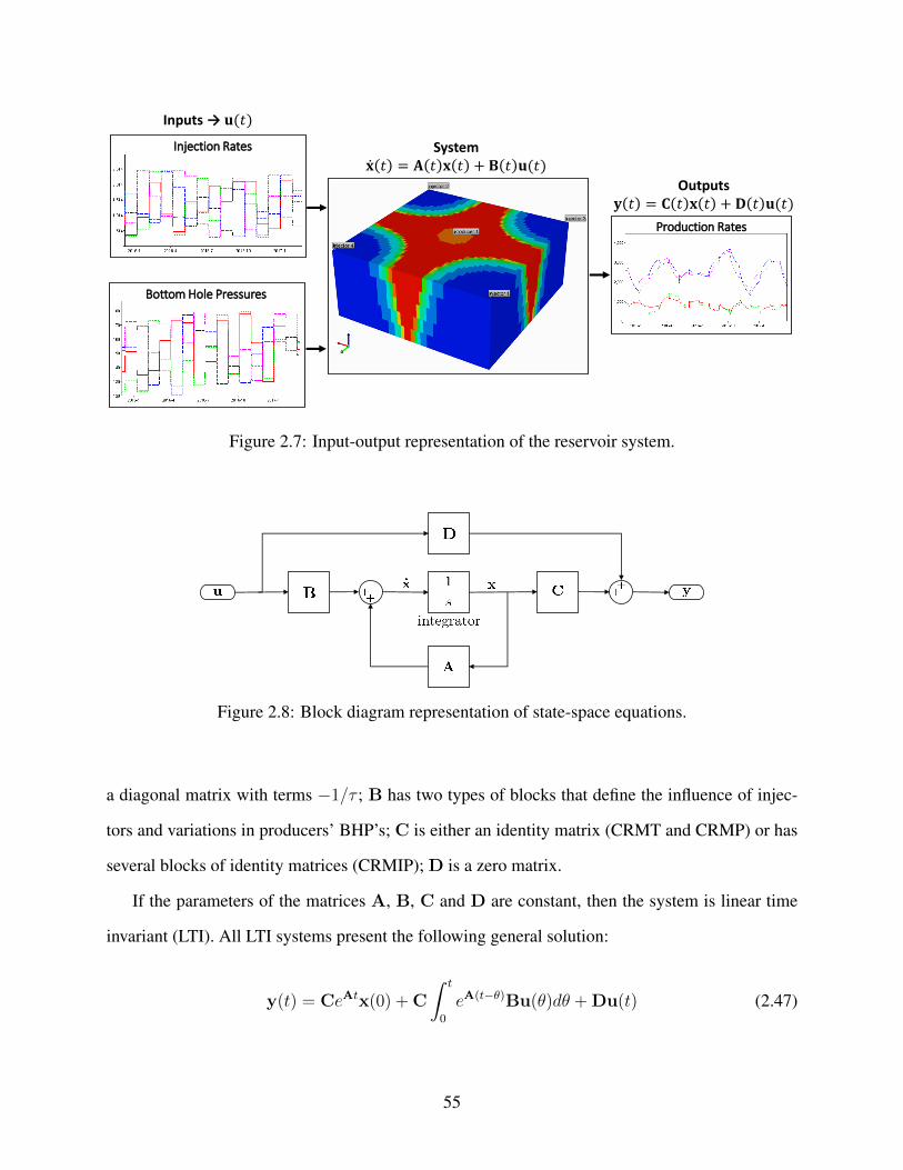
Injection Rates

Production Rates

Bottom Hole Pressures

Inputs → 𝐮(𝑡)

System 𝐱 𝑡 = 𝐀 𝑡 𝐱 𝑡 + 𝐁 𝑡 𝐮(𝑡)

Outputs𝐲 𝑡 = 𝐂 𝑡 𝐱 𝑡 + 𝐃 𝑡 𝐮(𝑡)

Figure 2.7: Input-output representation of the reservoir system.

Figure 2.8: Block diagram representation of state-space equations.

a diagonal matrix with terms −1/τ ; B has two types of blocks that define the influence of injec-

tors and variations in producers’ BHP’s; C is either an identity matrix (CRMT and CRMP) or has

several blocks of identity matrices (CRMIP); D is a zero matrix.

If the parameters of the matrices A, B, C and D are constant, then the system is linear time

invariant (LTI). All LTI systems present the following general solution:

y(t) = CeAtx(0) + C

∫ t

0

eA(t−θ)Bu(θ)dθ + Du(t) (2.47)

55

In other words, this is a general solution for the CRM representations when the parameters are

considered constant. In the above equation the first term represents the influence of primary pro-

duction, the second term is the convolution of the input signals (superposition of injection rates

and producers’ BHP’s variations), and the third term is zero.

These MIMO linear systems can also be represented in the Laplace space, where the systems

transfer function G(s) defines the relationship between the input U(s) and output Y(s) signals:

Y(s) = G(s)U(s) (2.48)

where s is the Laplace variable. Transfer functions (Laplace domain representation) and state-

space equations (time domain representation) are interchangeable:

G(s) = C(sI−A)−1B + D (2.49)

where I denotes the identity matrix.

Holanda [2015] derived transfer functions for the CRMT, CRMP, CRMIP and CRMIP-block.

Sayyafzadeh et al. [2011] proposed a first-order transfer function with time delay to model the pro-

duction response in waterflooding reservoirs when producers’ BHP’s are constant. As discussed

by Holanda [2015], the added time delay can be considered as an approximation for high order

transfer functions (blocks in series), therefore their model is similar to the CRM-block representa-

tion.

Representing CRM as state-space equations or transfer functions enables the application of

systems identification and control algorithms, which are valuable under specific workflows. For

example, Van Essen et al. [2013] proposes a model predictive control structure that integrates grid-

based reservoir simulation and low-order linear models to control the optimal trajectories of the

inputs, mitigating the impact of the uncertainty of the geological model. In this context, the CRM

would be an useful tool for the design of a fieldwide controller for production rates, this might

still require further model reduction to obtain a controllable and observable representation of the

56

system, as discussed by Holanda et al. [2015].

2.12 Case studies comparing CRM interwell connectivities with streamline allocation fac-

tors†

Izgec and Kabir [2010a] and Nguyen [2012] provide an interpretation of the interwell con-

nectivity using streamlines. According to their results, fij’s are a proxy for streamline allocation

factors, which are defined as the fraction of injected fluid conducted by the streamtubes starting

at injector i and ending on producer j. Therefore, any change in the streamlines (e.g. caused by

fluctuating rates and BHP’s or well shut-in) results in varying allocation factors. As depicted by

Izgec and Kabir [2010a], the constant values obtained from the CRM history matching correspond

to average values within the time span analyzed.

Although frequently CRM-derived interwell connectivities resemble streamlines allocation fac-

tors, these values might be noticeably different for some injector-producer pairs. Therefore, it is

important to emphasize that the CRM-derived interwell connectivities are mainly related to the

pressure support while streamlines allocation factors are related to the fraction of injected fluid

flowing towards a producer. As recently exemplified and discussed by Mirzayev et al. [2015]

for waterflooding in tight reservoirs, these differences can be further explored when studying the

distribution of flow paths and barriers in the reservoir.

Two examples are presented here to further discuss similarities and differences between CRM

interwell connectivities (fij’s) and streamline allocation factors (ψij’s), and are fully described in

Holanda et al. [2018d]. The first case is a 5 injectors and 4 producers (5×4) homogeneous reservoir

with flow barriers. Figure 2.9 shows the location of the flow barriers and compares maps for fij’s

and ψij’s.

An analysis was performed for every injector-producer pair considering the time varying be-

havior of ψij(t) and the assumption of constant fij . In Fig. 2.10, one can see that “INJ2”–“PROD3”

presents a very good agreement between ψij(t) and fij , indeed several injector-producer pairs be-

†The content of this section is reprinted with changes and with permission from "A generalized framework forCapacitance Resistance Models and a comparison with streamline allocation factors" by Holanda, Gildin, and Jensen,2018. Journal of Petroleum Science and Engineering, 162, 260-282, Copyright 2017 Elsevier B.V..

57

x(ft)0 500 1000 1500 2000 2500

y(ft

)

0

500

1000

1500

2000

2500

INJ1

INJ2

INJ3

INJ4

INJ5

PROD1

PROD2

PROD3

PROD4

fij=1

CRMIP

x(ft)0 500 1000 1500 2000 2500

y(ft

)

0

500

1000

1500

2000

2500

INJ1

INJ2

INJ3

INJ4

INJ5

PROD1

PROD2

PROD3

PROD4

Aij

=1Streamlines Allocation Factors (P50)

Figure 2.9: Maps for CRMIP connectivity (left) and median streamline allocation factor (right).The blue line depicts the low permeability barrier (kh = 1 md), the reservoir horizontal permeabil-ity (kh) is 200 md.

haved similarly. However, it is also important to notice that in some cases the differences can be

significant, with “INJ1”–“PROD2” being the extreme example. Also, there are cases when ψij(t)

presents a large variance, “INJ3”–“PROD2” (Fig. 2.10) and “INJ3”–“PROD4” are the largest ones.

The majority of w3(t) is allocated to “PROD2” and “PROD4” with large oscillations induced by

variations in w1(t) and w5(t).

f ij

3800 4000 4200 4400 4600 4800 50000.0

0.2

0.4

0.6

0.8

1.0INJ2-PROD3

3800 4000 4200 4400 4600 4800 50000.0

0.2

0.4

0.6

0.8

1.0INJ1-PROD2

3800 4000 4200 4400 4600 4800 50000.0

0.2

0.4

0.6

0.8

1.0INJ3-PROD2

time (days)

streamlines (ψij) CRMIP CRMP ICRM

Figure 2.10: Comparison between fij and ψij(t): good fit (left), largest difference (center) andlargest variance for ψij (right).

58

The streamlines simulation proved that for each injector the water is being allocated only to

the adjacent producers, which are within a 1500 ft spatial window (Fig. 2.9). However, when

such spatial window was applied to the CRM model, we realize that the quality of the history

matching significantly decreased. Therefore, it is important to physically distinguish fij and ψij .

Streamlines simulation computes the trajectories of the fluids in the porous media and can be used

to monitor the advance of the water front. The CRM interwell connectivities are computed solely

from the production response to changes in the injection rates. This is associated with the diffusion

of pressure in the porous media, which also happens in a significantly different time scale from the

advance of the flooding front. This reasoning is also helpful to distinguish time constants (τ ) from

time of flight. Thus, the injected fluids can still pass through the low permeability barrier as well

as the liquid production rates can be affected by variations in injection rates from a certain injector

without having the streamlines from such injector landing on the producer, as can be realized in

Fig. 2.9.

The second example is a 8×7 fluvial environment reservoir consisting of a sequence of braided

channels (Fig. 2.6a), which is based on layers 80 to 85 of the SPE-10 model [Christie and Blunt,

2001]. The width, orientation and format of these channels can vary significantly over geological

time, resulting in high vertical contrast, which impacts fluid flow. Furthermore, there is a high

areal contrast between channel and non-channel facies. Figure 2.11 shows the maps for CRMIP

connectivities and streamline allocation factors overlaying the reservoir heterogeneity, which is

represented by the log(kh × h(md× ft)) contours.

The analysis of the dynamic streamline allocation factors showed that most of the injected

fluid is being allocated to the neighboring producers, i.e. within the 1500 ft spatial window, at

most 0.7% of the fluid from a certain injector would be allocated to producers beyond this spatial

window. On the other hand, the CRM models presented an average for all of the injectors of

22.2% of pressure support provided to producers beyond the 1500 ft spatial window and 3.5% to

producers beyond the 2500 ft spatial window. Figure 2.12 presents a comparison of fij’s and ψij’s

for some injector-producer pairs.

59

INJ1 INJ2

INJ3

INJ4 INJ5

INJ6

INJ7 INJ8

PROD1

PROD2 PROD3

PROD4

PROD5 PROD6

PROD7

fij=1

CRMIP

x(ft)0 500 1000 1500 2000 2500 3000

y(ft

)

0

500

1000

1500

2000

2500

3000

3500

4000

4500

5000

5500

0

0.5

1

1.5

2

2.5

3

3.5

4

4.5

5

INJ1 INJ2

INJ3

INJ4 INJ5

INJ6

INJ7 INJ8

PROD1

PROD2 PROD3

PROD4

PROD5 PROD6

PROD7

Aij=1

Streamlines Allocation Factors (P50)

x(ft)0 500 1000 1500 2000 2500 3000

y(ft

)

0

500

1000

1500

2000

2500

3000

3500

4000

4500

5000

5500

0

0.5

1

1.5

2

2.5

3

3.5

4

4.5

5

Figure 2.11: Maps for CRMIP connectivity (left) and median streamline allocation factor (right).The contours show the log(kh×h(md× ft)) values, which represents the reservoir heterogeneity.

f ij

2600 2800 3000 3200 3400 3600 3800 40000.0

0.2

0.4

0.6

0.8

1.0INJ1-PROD1

2600 2800 3000 3200 3400 3600 3800 40000.0

0.2

0.4

0.6

0.8

1.0INJ5-PROD4

2600 2800 3000 3200 3400 3600 3800 40000.0

0.2

0.4

0.6

0.8

1.0INJ3-PROD1

time (days)

streamlines (ψij) CRMIP CRMP ICRM

Figure 2.12: Comparison between fij and ψij(t): good fit (left), largest difference (center) andlargest variance for ψij (right).

60

The connectivity maps (Figs. 2.9 and 2.11) are capable of detecting the transmissibility trends

in the reservoir, and fij accounts for the pressure support that a given producer receives from an

injector. This is directly related to the facies distribution. When there are transitions between facies

in the interwell flow path, the poor facies act like barriers, while the good quality facies (channels)

provide a continuous flow path. Therefore, the producer wells with larger connectivities are usu-

ally located in the good quality and continuous facies. On other hand, the streamline allocation

factors, ψij(t), define the fraction of injected fluid flowing towards a producer in a given time. The

difference between ψij and fij is beneficial for describing heterogeneity. For instance, available

tracer data in a field provides a clue of average ψij over time, which is related to the streamlines tra-

jectories, the CRM analysis would add valuable information in terms of the continuity of the good

facies for more distant injector-producer pairs, instead of just repeating the same information.

The fij’s and ψij’s present a good correlation in general, but also can be significantly different

(Figs. 2.10 and 2.12). These results challenge the application of fractional flow models with CRM

[Liang et al., 2007, Cao et al., 2015], because of the common misconception that fij are equivalent

to ψij , which can generate misleading results in the optimization of injected fluid allocation. A

simple way to obtain more reliable optimization results is to compute the water cut using fractional

flow with CRM in a reduced spatial window while a larger spatial window is used to compute the

total liquid rates.

2.13 Unresolved issues and suggestions for future research

Despite the efforts over the last decade to widen the range of applicability of CRM’s, there are

still some generic limitations in these models, as in any type of model. For practical purposes,

these limitations serve as indicators that help to identify situations when other modeling solutions

(e.g. streamlines simulation) should be pursued from the beginning of the analyses. For research

purposes, understanding and addressing these limitations can lead to new, more robust, practical

models.

61

2.13.1 Gas content of reservoir fluids

CRM’s assume that the reservoir fluids are undersaturated and slightly compressible. For this

reason, reservoirs with a gas cap, or where wells are experiencing gas coning are automatically

excluded from CRM case studies. Therefore, in future works, it would be interesting to test the

accuracy of the current models, and develop solutions capable of accommodating such cases.

In the cases of gas injection, the total compressibility is a function of reservoir pressure and

saturation, which possibly causes significant variations in time constants (Eq. 2.4) and productiv-

ity indices during the history matching and forecasting windows. However, some field applica-

tions did not present a specific formulation to address this issue during gas injection [Sayarpour,

2008, Salazar et al., 2012, Yin et al., 2016], and still obtained satisfactory results for the analysis

performed, suggesting that, in some cases, it may not be necessary to consider the time-varying

behavior of the parameters. For example, at supercritical conditions, carbon dioxide behaves like

a liquid [Eshraghi et al., 2016]. Laochamroonvorapongse et al. [2014] proposes to segment the

history matching window to capture events that are expected to cause significant variations in the

parameters. This is a valid approach to analyze how the parameters are evolving with time, but it

has limited predictive capability. Additionally, Nguyen (2012, Chap. 6) introduces a more complex

fractional flow model for water-CO2 flooding that incorporates relative permeability effects.

Despite the expected time-varying behavior of τ ’s and J’s, many times the circumstances might

be that producers are operated at nearly constant minimum bottomhole pressure during the selected

time window, which eliminates the need to estimate J ; while the history matching objective func-

tion (Eq. 2.21) is generally less sensitive to τ ’s than to fij’s [Jafroodi and Zhang, 2011, Kaviani

et al., 2014, Holanda et al., 2018d]. Under these circumstances, the time varying behavior of τ ’s

and J’s might not be noticed. This is a topic that deserves attention in future research, it is nec-

essary to perform a thorough sensitivity analysis using a set of grid-based reservoir models for

validation in order to define ranges of reservoir parameters controlling the applicability of CRM to

gas flooding; similar to the approach of Kaviani et al. [2014] for waterflooding.

62

2.13.2 Rate measurements

Even though the CRM equations assume that the flowrates are at reservoir conditions, fre-

quently these values are input at surface conditions. The cause of this problem might be that

flowrates are measured at the separator if a multiphase flowmeter is not incorporated in the well-

heads. This issue is easy to solve if formation volume factors and average reservoir pressure

estimates are available. A more complicated problem is when the flowrate measurements avail-

able are for the commingled production of some wells. In these cases, it is common to assume an

allocation factor to separate the production from each well, which does not honor the reservoir dy-

namics. Indeed, a more robust approach would be a coupled simulator of CRM and the production

system (nodal analysis).

2.13.3 Well-orientation and completion type

Although most examples that compare CRM with grid-based reservoir models are based on

fully penetrating vertical wells, this is not a model assumption. The CRM’s simply assume material

balance within a network structure, the fluid flow aspects related to well-orientation and completion

type are not explicitly considered. Stated differently, the time constant parameter (τ ) contains

the well productivity index; therefore, the well-orientation issue does not arise explicitly. In this

context, the following studies applied CRM in more specific cases:

• horizontal wells – Soroush (2013, Chap. 4), Mirzayev et al. [2017], Sayarpour (2008, p.

120), Almarri et al. [2017], Olsen and Kabir [2014];

• slanted wells – Soroush (2013, Chap. 4);

• partially-penetrating wells – Yousef et al. [2009].

In fact, the well geometry plays an important role while trying to interpret interwell connectiv-

ities and establish their relationship to reservoir geology. For vertical wells, the near-well region is

more influential than the interwell region on connectivity. This was used to detect wormhole de-

velopment [Soroush et al., 2014]. To reduce the dependency of the connectivities on the near-well

63

geometry and rock properties, Soroush [2013] proposed two approaches:

• The reverse-CM, wherein the injection rates are history matched while the production rates

serve as input variables.

• Subtracting the homogeneous connectivity calculated by the multiwell productivity index

(MPI) approach to obtain a ‘geometry adjusted’ connectivity.

Soroush et al. [2014] also proposed the compensated CM which allows for skin changes, which can

be a cause for apparent productivity index changes. For horizontal wells, the connectivity-geology

relation is more strongly related to the interwell features, this factor enabled correlation of seismic

impedance to connectivity in Mirzayev et al. [2017]. Therefore, as in these previous studies, it is

important to consider well-orientation and completion type while analyzing the results.

2.13.4 Time-varying behavior of the CRM parameters

In order to improve robustness of CRM’s, a valid attempt is to capture and model the time

varying behavior of their parameters as flooding evolves and flow patterns change. As previously

discussed, some developments already have been done [Jafroodi and Zhang, 2011, Moreno, 2013,

Cao et al., 2014, Lesan et al., 2017], however there is not a general formulation that is well accepted

yet. For example, shut-in wells remain as a problem, while the compensated CM [Kaviani et al.,

2012] is useful for more reliable interwell connectivity estimates and history matching, it is not

predictive. Although generalization problems are quite challenging, this is a recommended subject

for future research where theory and algorithms from pattern recognition and machine learning can

be helpful. In this context, there are many avenues to be explored which might improve accuracy

and account for model uncertainty. Many algorithms honor the physical aspects of the models, for

example, Bayesian techniques; this is a fundamental aspect to consider before selecting algorithms.

2.13.5 CRM coupling with fractional flow models and well control optimization

The coupling of CRM and fractional flow models assumes that interwell connectivities are

equivalent to streamline allocation factors. The previous comparisons [Nguyen, 2012, Izgec and

64

Kabir, 2010a] show that there is usually a fair correlation between these two parameters, how-

ever for some injector-producer pairs the differences might be significant [Mirzayev et al., 2017,

Holanda et al., 2018d]. This impacts the oil production forecasts and optimization results. There-

fore, a suggestion to future works is to develop more consistent coupling of CRM and fractional

flow models in a way that is capable of identifying and correcting the well pairs that present such

discrepancies.

Hong et al. [2017] compared the optimization results from CRM and grid-based reservoir

simulation, proposing a methodology to integrate both models, reducing computational time and

checking the reliability of CRM as a proxy-model. Their results indicated that CRM provided near-

optimal results for the reservoir models analyzed in their case studies. In optimization studies, this

comparison with grid-based reservoir models to assess the optimality of the proposed solutions

is fundamental to provide more confidence, and must become a common practice. Additionally,

it may be important to have the capability of considering simultaneously primary and secondary

constraints (flowrates, bottomhole pressures, and water cut) to monitor injectivity issues, fracturing

pressures, gas coning and economic limits while optimizing control.

2.13.6 Unconventional reservoirs

As discussed in this chapter, the CRM’s have been mainly applied to conventional reservoirs.

It is important to mention that there has also been previous attempts to extend these concepts to

unconventional reservoirs. For example, Kabir and Lake [2011] applied the CRM-block solution

to capture the long transient period of the production decline during the primary depletion, and

Mirzayev et al. [2017] presented a case study of waterflooding in tight formations. However, the

previous models did not explicitly account for the linear flow and the pressure diffusion associated

with the extended transient period during the primary recovery in unconventional reservoirs.

In fact, many of the unresolved issues previously discussed arise when dealing with uncon-

ventionals: 1) a considerable portion of the production is from gas reservoirs; 2) publicly avail-

able monthly production data is abundant, but can be erratic and/or sampled at a lower frequency

than desired; 3) in these multistage hydraulically fractured horizontal wells the well orientation

65

and completion type affect directly the fluid flow and, consequently, the production profile; and

4) since the permeability is very low, the extended transient period implies that the investigated

reservoir volume increases with time until the onset of boundary dominated flow. Therefore, it

is necessary to incorporate these aspects of the physics of fluid flow in multistage hydraulically

fractured wells in unconventional formations while keeping the models simple, i.e., with a reduced

number of parameters. Chapter 3 introduces the θ2 model to address these issues.

66

3. A PHYSICS-BASED DECLINE MODEL FOR UNCONVENTIONAL RESERVOIRS∗

This chapter introduces the mathematical derivation of the θ2 decline model, which accounts for

material balance and linear flow while still incorporating some empiricism in the functional form

to accommodate further complexities observed in field data. It can be considered an extension

of CRM to unconventional reservoirs because the mathematical derivation starts from the CRM

material balance equation. The θ2 model always has a finite EUR and only 3 parameters to be

estimated from the production history. Additionally, this chapter also introduces the formulations

for history matching, uncertainty quantification, data filtering and probabilistic calibration to obtain

production forecasts and EUR with the θ2 decline model using only publicly available production

data.

3.1 Physics: Jacobi theta function no. 2 as a decline curve model

3.1.1 Model derivation

The model proposed here is obtained by coupling the material balance equation with the pres-

sure solution for the homogeneous linear one dimensional reservoir depicted in Fig. 3.1. The

governing equations and boundary and initial conditions are similar to the ones presented in Ogun-

yomi et al. [2016], however the model is simplified by assuming an infinitely conductive fracture.

For a reservoir under primary production, the material balance equation for the drainage volume

of each well can be written as:

Vpctdp

dt= −q (3.1)

where p is the average reservoir pressure, q is the production rate, Vp is the drainage pore volume

and ct is the total compressibility of the system.

∗The content of this chapter is reprinted with minor changes and with permission from: 1) "Combining Physics,Statistics and Heuristics in the Decline-Curve Analysis of Large Data Sets in Unconventional Reservoirs" by Holanda,Gildin, and Valkó, 2018. SPE Reservoir Evaluation & Engineering, 21(3), 683–702, Copyright 2018 Society ofPetroleum Engineers; and 2) "Probabilistically Mapping Well Performance in Unconventional Reservoirs with aPhysics-Based Decline Curve Model" by Holanda, Gildin, and Valkó, 2019. SPE Reservoir Evaluation & Engi-neering, Copyright 2019 Society of Petroleum Engineers.

67

a) b)

Figure 3.1: a) Representation of a horizontal well with evenly spaced hydraulic fractures. Thedashed red box indicates the symmetric element considered in the derivation of the θ2 model.b) Top view of the symmetric element with diffusivity equation and initial and boundary conditions.The hydraulic fractures are assumed to be infinitely conductive.

The definition of average reservoir pressure is modified to:

p(t) =1

L

∫ L

xi

p(x, t)dx (3.2)

where 0 ≤ xi ≤ L instead of xi = 0. The reason for this modification is that it allows the model to

have an initial delay and buildup in the production response, which is often observed in field data

due to several physical or operational reasons, as it will be further discussed. This is an empirical

aspect introduced to the previous model of Wattenbarger et al. [1998], thus it is emphasized that xi

does not have an explicit physical meaning.

The derivation of the solution for the pressure distribution in the matrix domain over time,

p(x, t), is presented in Appendix A. Substituting Eq. A.30 in Eq. 3.2 and after solving the integral,

the following expression is obtained:

p(t) = pwf +∞∑n=0

8

π2

(pi − pwf )(1 + 2n)2

e−κ(π2L

(1+2n))2t cos

(π2

xiL

(1 + 2n))

(3.3)

The drainage pore volume is defined as:

Vp = φAL (3.4)

68

and the diffusivity constant as:

κ =k

φµct(3.5)

Applying Eqs. 3.3, 3.4 and 3.5 in Eq. 3.1, the following expression is obtained after the proper

algebraic manipulation:

q(t) =kA

µL(pi − pwf )

∞∑n=0

2e− kφµct

( π2L

(1+2n))2tcos(π

2

xiL

(1 + 2n))

(3.6)

The mathematical representation of this model can be simplified based on the second Jacobi theta

function, which is defined as follows:

θ2 (u, v) = 2∞∑j=0

v( 1+2j2 )

2

cos (u(1 + 2j)) (3.7)

In the θ2 decline model, there are only three lumped parameters for the history matching of the

observed monthly production. q∗i is the virtual initial rate, and is equivalent to the transmissibility

at the fracture face multiplied by the initial pressure drawdown:

q∗i =kA

µL(pi − pwf ) , (3.8)

χ is a parameter introduced to allow an initial delay and buildup in the production rates or simply

a deviation from the negative half slope of transient flow:

χ =π

2

xiL, (3.9)

and η is the reciprocal characteristic time, which is related to the diffusivity constant of the reser-

voir:

η =π2

L2

k

φµct. (3.10)

69

Therefore, Eq. 3.6 can be written in a simpler way as the second Jacobi theta function (θ2):

q(t) = q∗i θ2

(χ, e−ηt

)(3.11)

χ is named as “geometric factor” because it is expressed only in terms of variables with di-

mension of length (xi and L). However, for the same reasons previously stated for xi, an explicit

physical interpretation is not attributed to χ, but there are a variety of factors that cause χ 6= 0, as

it will be further discussed.

As exemplified above, the Jacobi theta functions are intrinsically related to the analytical solu-

tion of certain partial differential equations. For this reason, these functions also have been applied

in other fields of science and engineering, such as heat transfer [Chouikha, 2005], cosmology

[D’Ambroise, 2010] and quantum field theory [Tyurin, 2002]. The main concern in applying Eq.

3.11 in the decline curve analysis of large datasets is the fact that it is an infinite summation, how-

ever there are computational routines available that are capable of computing it in a time effective

manner [Wolfram Research, Inc., 1988, Igor, 2007, Johansson et al., 2013].

The θ2 model has been derived for liquid rates. Even though a strict physical derivation might

be unfeasible for the gas case, this model has also been validated with field data in gas wells (chap-

ter 4). Moreover, Al-Hussainy et al. [1966] proved that the solutions to the diffusivity equation for

gas and liquid have a similar format when using pseudo-pressure function in the gas case, assuming

φµ(p)ct(p))k

is constant. On the other hand, the material balance equation is intrinsically related to the

definition of isothermal compressibility, which is expressed in terms of average reservoir pressure

instead of a pseudo-pressure function. Furthermore, it is necessary to assume that Vpct is constant,

as well as to compute average reservoir pressure from the pseudo-pressure solution. Therefore, it

seems to be impossible to pursue such derivation without making several hard assumptions. On the

other hand, it is also important to emphasize that the behavior of the θ2(0, e−ηt) model proposed by

Wattenbarger et al. [1998] has been observed in a number of gas wells. Additionally, the empirical

models (e.g. Arps hyperbolic, stretched exponential and Duong) are usually applied in the industry

70

without distinction whether the fluid is oil or gas.

3.1.2 Subcases and extensions of the θ2 model

3.1.2.1 Wattenbarger et al. [1998]

If χ = 0, the solution presented in Eq. 3.11 is equivalent to the one introduced by Wattenbarger

et al. [1998] for tight reservoirs, and derived in Carslaw and Jaeger [1959] for linear heat conduc-

tion problems. It has only two parameters, is valid for transient and boundary dominated flow and

presents a continuous decline. Easley [2012] proposed an approximation function to θ2 (0, e−ηt)

that does not require to evaluate the infinite summation term.

3.1.2.2 Double-porosity model [Ogunyomi et al., 2016]

Ogunyomi et al. [2016] proposed a rate-time relationship by coupling material balance and the

analytical solution for pressure (Eq. A.30) in a double-porosity system. Their model is a time do-

main approximation of the Laplace space solution proposed by Bello [2009]. It assumes a constant

pressure at the fracture face due to the high contrast in the permeability at the fracture/matrix in-

terface, which causes pressure to reach a quick equilibrium with pwf in the fracture compartment.

Based on this assumption and the material balance equations presented by Ogunyomi et al. [2016],

the double-porosity model can be recast in terms of θ2 functions as:

q(t) = q∗i,mθ2

(0, e−ηmt

)+ q∗i,fθ2

(0, e−ηf t

)(3.12)

where the subscripts m and f refer to the matrix and fracture compartments, respectively.

Figure 3.2 shows the double-porosity θ2 approximation. Notice that this model has four pa-

rameters, which can be a problem when dealing with sparse data, such as the monthly reported

production rates. If the fracture boundary effect happens before the end of the first month of pro-

duction, the parameters related to the fracture control volume, i.e. q∗i,f and ηf , will be overfitting the

production history and not improving the predictions. In this case, the model requires production

rate measurements at a higher frequency. For typical values of these parameters in unconventional

71

resevoirs, it is expected that the transition from fracture to matrix transient flow to happen in the

order of minutes while monthly reported production is the data analyzed in this work. Therefore,

the assumption of infinitely conductive fracture is plausible here.

fracture transient

flow

fracture

boundary

effect

matrix

transient

flow

matrix

boundary

effect

Figure 3.2: The double-porosity model approximation in terms of θ2 functions. q∗i is inmcf/month and η is in month−1.

3.1.3 Comparison with the Arps decline model

The Arps [1945] decline curves family has been widely applied in the industry to estimate

reserves. This practice also has been extended to unconventional reservoirs [Gong et al., 2014],

where the hyperbolic model is the most suitable to capture the production decline during the tran-

sient state:

q(t) = q∗i (1 + bDit)− 1b (3.13)

where q∗i is the initial rate (q(0)), b is the decline exponent and Di is the initial decline rate.

Figure 3.3 shows the sensitivity of the production decline profile in a log-log plot when varying

the Arps parameters b and Di. In Fig. 3.3a, notice that as b increases the slope varies significantly

less when comparing early and late time. In Fig. 3.3b, the different values of Di present only

72

a slight difference in the early time, while in the late time the profile is similar (parallel straight

lines), then varying q∗i is equivalent to vary Di in this case.

b=0.001

b=0.401

b=0.801

b=1.2

b=1.6

b=2.

1 5 10 50 1000.001

0.005

0.010

0.050

0.100

0.500

1

time (months)

Dimensionlessproductionrate

(qD)

(a) (1+b Di t)-1b , Di=0.1

Di=0.1

Di=0.25

Di=0.63

Di=1.58

Di=3.98

Di=10.

1 5 10 50 1000.001

0.005

0.010

0.050

0.100

0.500

1

time (months)

Dimensionlessproductionrate

(qD)

(b) (1+b Di t)-1b , b=1.82

Figure 3.3: Sensitivity to: (a) b and (b) Di parameters in the Arps hyperbolic model. In each plotone of the parameters is fixed at the median value of the best fit solutions for the 992 Barnett gaswells presented in chapter 4. Di is in month−1 and qD(t) = q(t)/q∗i .

Figure 3.4 presents a sensitivity to the parameters η and χ in the θ2 model. The production

profiles must be compared with the ones in Fig. 3.3. Notice that the θ2 model captures the half slope

73

of the transient flow regime and presents a transition to the boundary dominated flow, achieving

the exponential decline. In Fig. 3.4a, varying the reciprocal characteristic time (η) is equivalent to

shifting the production profile horizontally, while varying q∗i is equivalent to shifting it vertically.

As one can see in Fig. 3.4b, the geometric factor (χ) is the one that defines the shape of the curve,

adding flexibility to the model presented by Wattenbarger et al. [1998].

The parameter χ allows the model to have an initial delay and buildup in the production rates.

This feature is also present in the Duong [2011] and the stretched exponential [Valkó, 2009, Valkó

and Lee, 2010] models. In general, χ can be interpreted as a deviation from the assumptions of

the Wattenbarger et al. [1998] model. Such deviation can be related to the reservoir physics or

field operations. An example of physical reason is that as the reservoir starts to be depleted, pore

pressure declines and the effective stress (σes) increases. If σes exceeds the strength of the shale,

the fractures are reactivated, propagating and causing the initial buildup in the production rates

[Duong, 2011]. Another plausible physical reason is that a variable skin factor due to cleanup of

drilling fluids and unloading gas condensate while starting production can cause this initial increase

[Larsen and Kviljo, 1990, Clarkson et al., 2013, Hashmi et al., 2014]. Operational factors can also

contribute to an increasing q(t) in the production history, such as long shut-in time during part of

the sampling period, oil price fluctuations, restimulation and gas condensate unloading operations.

Therefore, the χ parameter improves the model’s flexibility, which is a desirable feature when

dealing with a more complex production history.

As proved by Lee and Sidle [2010], the Arps’ curves family has the problem that the esti-

mated ultimate recovery (EUR) is infinity when b ≥ 1 and no economical or time constraints

are imposed, i.e. limt→∞∫ t

0q(t)dt= ∞, which is physically impossible. In such cases, the Arps

hyperbolic model should not be applied for long-term forecast because the observed data only ex-

hibits transient flow or other nuances of the production mechanism and the model does not present

a transition to boundary dominated flow embedded in its functional form. In contrast, Appendix D

presents a general proof that the θ2 model has a finite EUR and a simple equation for the special

case of χ = 0.

74

η=0.01

η=0.022

η=0.048

η=0.105

η=0.229

η=0.5

-1/2 slopeexponential

decline

1 5 10 50 100 500 10000.001

0.010

0.100

1

time (months)

Dimensionlessproductionrate

(qD)

(a) θ2(χ, ⅇ-η t), χ=0.22

χ=0.05

χ=0.34

χ=0.63

χ=0.92

χ=1.21

χ=1.5

exponential

decline-1/2 slope

1 5 10 50 100 500 10000.001

0.050

1

time (months)

Dimensionlessproductionrate

(qD)

(b) θ2(χ, ⅇ-η t), η=0.053

Figure 3.4: Sensitivity to: (a) η and (b) χ parameters in the θ2 model. In each plot one of theparameters is fixed at the median value of the best fit solutions for the 992 Barnett gas wellspresented in chapter 4. The half slope indicates transient flow and the exponential decline indicatesboundary dominated flow. η is in month−1 and qD(t) = q(t)/q∗i .

75

Table 3.1: Theoretical and practical box constraints in the θ2 and Arps hyperbolic models. η andDi are in month−1.

θ2 Arps hyperbolic

Theoretical Practical Theoretical Practical

η ≥ 0 0.01 ≤ η ≤ 0.5 Di ≥ 0 0.1 ≤ Di ≤ 12

0 ≤ χ ≤ π/2 0.05 ≤ χ ≤ 1.5 0 ≤ b ≤ 2 0.001 ≤ b ≤ 2

q∗i ≥ 0 0.05 ≤ q∗i /qmax ≤ 2 q∗i ≥ 0 0.05 ≤ q∗i /qmax ≤ 3

3.2 History matching

The best fit model is obtained by solving a least squares problem with the following objective

function:

min z = min(log qobs − log qpred)TC−1e (log qobs − log qpred) (3.14)

where qpred and qobs ∈ <Nt×1 and are vectors of the production rates predicted by the model

and observed in the production history, respectively; Ce ∈ <Nt×Nt and is the covariance matrix of

the measurement and modeling errors, which is discussed in more details in Section 3.4; Nt is the

number of time steps. Since q(t) can have different orders of magnitude in the same production

history, log q(t) is considered in the objective function.

Table 3.1 presents the box constraints for the θ2 and Arps hyperbolic models, where the “prac-

tical” constraints were the ones applied to the case study in chapter 4. In the θ2 model, even

with these box constraints, occasionally a negative q(t) is computed, adding the following linear

constraint is a simple way to solve this problem (η is in month−1):

χ ≤ 12η (3.15)

Figure 3.5a shows this constraint in the χ vs. η solution space, the dots represent the best fit θ2

models for the 992 Barnett gas wells (chapter 4). Figure 3.5b confirms a fair correlation between

q∗i and qmax, which allows to define the box constraints in terms of q∗i /qmax (Table 3.1).

76

χ > 12 η

0.1 0.2 0.3 0.40.0

0.2

0.4

0.6

0.8

1.0

1.2

1.4

η (month-1)

χ(d

imen

sion

less

)

(a) χ vs. η - Solution Space

5000 1× 104 5× 104 1× 105

5001000

50001× 104

5× 1041× 105

Maximum production rate (mcf/month)

qi*(mcf/month)

(b) qi* vs. qmax

Figure 3.5: Best fit solutions for the 992 Barnett gas wells with the θ2 model: (a) distribution in theχ vs. η space, the yellow area depicts the linear constraint; (b) relationship between q∗i and qmax.

3.3 Statistics: uncertainty quantification

3.3.1 Bayes theorem

While analyzing production data to forecast reserves, it is preferable to proceed with a proba-

bilistic rather than deterministic approach so that risk awareness is improved before decisions are

taken. The Bayes’ theorem has been widely used for uncertainty assessment and data integration in

reservoir engineering problems [Oliver et al., 2008, Gong et al., 2014]. It reconciles the following

77

elements: expert’s judgment, embedded in the prior distribution, Ppr(Ψj); and the value of data

acquired and model proposed, embedded in the likelihood function, Pl(qobs|Ψj). Thus, the Bayes’

theorem provides the posterior distribution of the parameters:

Ppost(Ψj|qobs) =Pl(qobs|Ψj)Ppr(Ψj)∫Pl(qobs|Ψ)Ppr(Ψ)dΨ

(3.16)

where Ψj is a vector with candidate values for each parameter of the decline model (e.g. Ψj =

[η, χ, q∗i ]Tj ).

Figure 3.6 illustrates the application of Bayes’ theorem in the estimation of the θ2 model pa-

rameters (3D space) for well 8 (Fig. 3.9). The color bar indicates the normalized values of the

probability distribution functions, with the hot colors being the most likely region for the θ2 pa-

rameters. Notice how the posterior is generated from the interplay between the prior distribution

and likelihood function.

3.3.2 Markov chain Monte Carlo (MCMC) algorithm

Analyzing Eq. 3.16, even when the prior and likelihood functions are expressed in a closed

form, the integral in the denominator might be very difficult or impossible to solve. For this

reason, sampling algorithms are frequently incorporated in a Bayesian framework, such that a large

enough sample that resembles the posterior distribution is generated without solving the integral.

From the percentiles of this sample it is possible to obtain the P10, P50 and P90 of a certain

property. The sampling method used in this work is the Markov Chain Monte Carlo (MCMC) with

the Metropolis algorithm. Here, the algorithm is briefly explained, for more theoretical details the

reader is referred to Gong et al. [2014] and Oliver et al. [2008]. Compared to Gong et al. [2014],

the only modifications made were to incorporate Ce and the linear constraint (Eq. 3.15) in their

framework.

For the likelihood function, it is assumed that the error between the proposed model and pro-

duction history, i.e. (log qobs − log qprop), follows a normal distribution with zero mean, i.e.

78

0

0.2

0.4

0.6

0.8

1.0

Figure 3.6: Bayes theorem idea applied to well 8 (API #: 42121329920000) with the new workflowand model. Normalized probability distribution function values are depicted by the color scale inthe 3 parameter solution space for: (a) prior, (b) likelihood, (c) posterior. η is in month−1 and q∗iis in mcf/month.

N (0, σbf ). This results in:

Pl(qobs|Ψprop) =1√

2πσbfexp

(−

σ2prop

σ2bf + ε

)(3.17)

79

where σbf is the standard deviation of the residual for the best fit model and is given by:

σbf =

(1

Nt − 3(log qobs − log qbf )

TC−1e (log qobs − log qbf )

)0.5

; (3.18)

σprop is the standard deviation of the residual for the proposed model, defined as:

σprop =

(1

Nt

(log qobs − log qprop)TC−1e (log qobs − log qprop)

)0.5

; (3.19)

and ε is the inherent error of the production data, which is introduced to avoid extremely small

acceptance ratios (αR) and consequently unrealistically low uncertainties. As successfully experi-

enced by Gong et al. [2014], ε = 0.001 is the value used here.

Then, a Markov chain is built. A model (Ψj,prop) is proposed from a proposal distribution. It

has αR probability of being accepted, i.e. being aggregated to the chain, and (1 − αR) of being

rejected, in which case the previous model (Ψj,s−1) is repeated in the chain. The acceptance ratio

(αR) is computed by comparing the posterior probabilities of Ψj,prop and Ψj,s−1.

Considering Eqs. 3.17, 3.18 and 3.19, as well as proposal distributions that are independent

truncated normal distributions for each parameter with bounds defined in Table 3.1, the acceptance

ratio is obtained from:

αR = min

1, exp

(σ2s−1 − σ2

prop

σ2bf + ε

)Ppr(Ψprop)

Ppr(Ψs−1)×

∏υ=η,χ,q∗i

ΦN

(υup−υs−1

συ

)− ΦN

(υlow−υs−1

συ

)ΦN

(υup−υprop

συ

)− ΦN

(υlow−υprop

συ

)

(3.20)

where υ represents each of the decline curve parameters; υup and υlow are the upper and lower

bounds (Table 3.1) for each parameter, respectively; συ is the standard deviation for each parame-

ter, which is estimated from the best fit solutions for the full dataset; and ΦN () is the cumulative

distribution function of the standard normal, N (0, 1).

The MCMC with the Metropolis algorithm applied to the θ2 model for a sample with size

nMCMC can be summarized as:

80

0. Set s = 1 and Ψs = Ψbf .

1. s = s + 1. Draw Ψprop from the proposal distribution, Ntruncated(Ψs−1, σΨbf), until it

satisfies Eq. 3.15.

2. Compute αR from Eq. 3.20.

3. Draw a random number, rn, from a standard uniform distribution, U(0, 1).

4. If rn < αR, then Ψs = Ψprop. Otherwise, Ψs = Ψs−1.

5. If s < nMCMC , then return to step 1. Otherwise, the Markov chain is complete.

3.3.3 The roles of the prior distribution and the likelihood function

Figure 3.7 shows an application of the probabilistic framework with the θ2 model and field data,

demonstrating how the choice of different prior distributions condition the posterior distribution

from which the uncertainty is quantified. Mathematically, the prior can be any probability density

function. In practice, it represents the expert’s judgment before data specific to the problem is

presented, i.e., the initial knowledge. It is desirable to have a representative prior that filters out

implausible values of the model parameters, and has embedded knowledge that enables to consis-

tently reduce the final uncertainty. On the other hand, one must be careful to not assign a prior

that is too restrictive, which potentially impairs the ability of the posterior distribution to also learn

from the behavior of the observed data through the likelihood function. Therefore, it is desirable

to systematically incorporate knowledge in the prior distribution, for example, considering typical

values of the decline model to a specific region. The algorithm presented in Sec. 5.2.2 provides a

mathematical framework with criteria established to generate a prior distribution that automatically

assimilates knowledge from previous results of other producing wells in the analyzed region. In

this context, the well placement problem is analogous to the challenge of defining a representative

prior, where no production history data for the well is available and reservoir engineers and geol-

ogists analyze potential locations based on other indicators and previous experiences, then, infer

performance while acknowledging the inherent risk involved in the decision making.

81

0

0.2

0.4

0.6

0.8

1.0

Figure 3.7: Application of the Bayes theorem to the θ2 model with two different prior distri-butions. The likelihood function considers the first 12 months of production data from wellAPI#4212133349. All probability distribution functions are normalized by their maximum val-ues and depicted by the color scale. η is in month−1 and q∗i is in mcf/month.

Figure 3.8 shows how the uncertainties in the likelihood function and, consequently, in the

posterior reduce as more production history becomes available with time. In unconventional wells,

the transient period is usually long and may last years due to the low matrix permeability. Since

the reciprocal characteristic time, η, basically defines the time for the transition from transient to

boundary dominated flow (tD = ηt ≈ 1.7), the likelihood function will indicate a high uncertainty

on η until boundary dominated flow is observed. Even if such transition is not observed, the uncer-

tainty in the likelihood function will gradually decrease as more production history is acquired, and

more evidence is provided that η should have a lower value. As the model response is dependent in

all parameters, the uncertainty of all of them is affected by this phenomena. Therefore, in uncon-

ventional reservoirs, it is not recommended to rely on a single history matched solution, as there

82

is a high risk that the EUR may not be representative of the potential production that the reservoir

is capable to deliver. A more robust approach is to reliably quantify the inherent uncertainty of the

forecasts while reconciling observed data and previous knowledge in the analyzed region. In this

context, the prior helps to guide the final result of the probabilistic analysis in conjunction with the

observed data, keeping results that are plausible according to the initial knowledge, and reducing

the probability of unlikely scenarios. While Eqs. 3.17-3.19 establish a formal basis to compute the

likelihood function, the prior is frequently left as a subjective choice based on the experience of

the engineer. Hence, it is important to propose criteria based on aspects influencing the reservoir

properties and fluid flow physics which can be easily assimilated and guide the definition of a prior

distribution.

0

0.2

0.4

0.6

0.8

1.0

Figure 3.8: Application of the Bayes theorem to the θ2 model considering the same priordistribution, but different lengths of production history for the likelihood function of wellAPI#4212133349. All probability distribution functions are normalized by their maximum val-ues and depicted by the color scale. η is in month−1 and q∗i is in mcf/month.

83

3.4 Heuristics: treating the bad data

Data processing for the application of decline curve analysis can be a tedious and subjective

task, specially when dealing with large datasets. Production data from unconventional wells can

present several discontinuities, which can be caused by physical processes, operations or other

non-stochastic factors. For example, increasing drawdown, unloading gas condensate or refrack-

ing operations will cause production to suddenly increase, shut-in a well for a half month for

pipeline maintenance results in a lower monthly production. This section introduces an automatic

and consistent way of dealing with erratic production histories and calibrating uncertainty of the

forecasts.

For this purpose, heuristic rules are defined to assign a weight, vi, to each data point in a

production history, q(ti). These weights are then incorporated in the covariance matrix of the

measurement and modeling error, Ce, in the history matching (Eq. 3.14) and uncertainty analysis

(Eqs. 3.18 and 3.19). The basic idea is that the value of the weight vi is a measure of the importance

and confidence on q(ti) for the forecast period. Following, each of the heuristic rules are presented

and explained in the sequence that they are implemented.

1. Start setting the vector of weights with unit elements:

vinitial = [v1, v2, ..., vi, ..., vNt ]T = 1Nt×1 (3.21)

2. Flowrates below a threshold value, qlim, are assigned zero weight, i.e. if q(ti) ≤ qlim, vi = 0.

This is necessary to eliminate unrealistically low flowrates that does not correspond to the

actual reservoir potential and deviates the models towards lower production rates. Now,

vinitial is a vector of zeros and ones.

3. Decline curve analysis is mostly concerned with propagating the last state of production, i.e.

higher weights must be assigned as time increases. Therefore, the weights can be redefined

84

as an increasing function of vinitial and ti:

v = [fv(v1, t1), ..., fv(vi, ti), ..., fv(vNt , tNt)]T (3.22)

In this paper, fv(vi, ti) is a linear function, so Eq. 3.22 can be written as:

v = avvinitialT t + bv (3.23)

4. It is common to have data points that when compared to the general production trend are

significantly deviated downwards, but are still higher than qlim, as shown in Fig. 3.9. There-

fore, it is important to reduce the contribution of these data points to the forecast, i.e. reduce

vi. For this reason, a straight line (unconstrained exponential model) is fit to the logarithmic

production history, log qobs, yielding:

log qexp(t) = aexpt+ bexp (3.24)

This line is shifted downwards by introducing the multiplier ml:

log qexp,l(t) = aexpt+mlbexp (3.25)

where 0 ≤ ml ≤ 1. This is the red dashed line shown in Fig. 3.9. If log qobs(ti) ≤

log qexp,l(ti), then vi is reduced by a multiplier 0 ≤ βm ≤ 1, such that vi = βmvi.

Once the weights (v) have been defined, they are introduced in Ce, such that C−1e is computed

as:

C−1e = Diag

[v1

(log qobs(t1))2, ...,

vi(log qobs(ti))2

, ...,vNt

(log qobs(tNt))2

], Ce ∈ <Nt×Nt (3.26)

The denominator is defined as (log qobs(ti))2 as a way to normalize the errors, thus dealing with

85

Out[278]=

productionrate

(mcf/month)

0 20 40 60 80100

5001000

50001× 104

5× 1041× 105

well 1, API#: 42097341450000

0 20 40 60 80100

5001000

50001× 104

5× 104well 2, API#: 42497369130000

0 20 40 60 80100

5001000

50001× 104

5× 1041× 105

well 3, API#: 42121341110000

0 20 40 60 80100

5001000

50001× 104

5× 104well 4, API#: 42497370630000

0 20 40 60 80100

5001000

50001× 104

5× 104

well 5, API#: 42097341950000

0 20 40 60 80100

500

1000

5000

104

well 6, API#: 42497369110000

0 20 40 60 80100

500

1000

5000

104

well 7, API#: 42497370560000

0 20 40 60 80100

500

1000

5000

1× 104

5× 104well 8, API#: 42121329920000

0 20 40 60 80100

500

1000

5000

104

well 9, API#: 42121338360000

time (months)

production history θ2 (best fit) filter line

Figure 3.9: Best fit solutions of the θ2 model using heuristic rules to filter the data.

relative errors in the history matching and uncertainty analysis. For numerical stability, if qobs(ti) ≤

qlim, it is redefined as qobs(ti) = qlim, remember that vi = 0 in this case.

3.4.1 Tuning the heuristics for uncertainty calibration

Even though the reasoning of heuristic rules have been previously explained and exemplified,

it is necessary to have a consistent procedure to define its parameters (av, bv, ml and βm). Here, the

criteria established is that such parameters must be defined in a way that calibrates the uncertainty

of the forecasts. Also, it is desirable that these parameters keep the uncertainty calibrated as more

production history is obtained and new forecasts are made.

For this purpose, the concept of hindcasts is used, where each production history is split in

two periods: the first period is used for model fitting; the second period is the blind data that is

compared with the forecast projected from the model generated with first period data. As done by

86

Gong et al. [2014], the total production during the second period (PDTSP, or Q2nd) is considered

as a metric for the calibration. Then, for the full dataset (e.g., 992 Barnett gas wells for the

case study of chapter 4) the frequency that the observed PDTSP is higher than the ones for a

predefined percentile model (e.g. P50 is the 50th percentile) is computed, which is here denoted as

ω(Q2nd,obs > Q2nd,percentile) and is the real percentile. The models are probabilistically calibrated if

ω(Q2nd,obs > Q2nd,percentile) match the predefined percentiles. Therefore, comparing the forecasts

and actual production history in a large dataset, it is possible to check if the projected percentiles

(e.g. P10, P50 and P90 models) correspond to the distribution of the actual dataset.

Considering the P10, P50 and P90 models, this can be framed as an optimization problem with

objective function depending on the heuristic parameters (av, bv, ml and βm):

minav ,bv ,ml,βm

∑th

(ωth(Q2nd,obs > Q2nd,P10)− 0.1)2 + (ωth(Q2nd,obs > Q2nd,P50)− 0.5)2

+(ωth(Q2nd,obs > Q2nd,P90)− 0.9)2

(3.27)

where th represents total time used in the first period, in the case study in chapter 4 it takes the

values 6, 12, 18, 24, 30 and 36 months. The following constraints were applied:

0.05 ≤ av ≤ 2 (3.28)

0.85 ≤ ml ≤ 1 (3.29)

0 ≤ βm ≤ 0.5 (3.30)

and bv = 0 was defined to reduce the number of parameters in the problem.

For comparison, Fig. 3.10 shows the need for probabilistic calibration in the base case, where

the heuristic rules are not applied (av = 0, bv = 1, ml = 1 and βm = 1). Figure 3.11 shows the

probabilistically calibrated case with the adjusted heuristic parameters, which is further discussed

in Chapter 4.

87

Out[556]=

10 15 20 25 30 350.0

0.2

0.4

0.6

0.8

1.0

Production data used to hindcast (months)

FrequencyofTruePDTSP>ProbabilisticPDTSP

θ2 - Best Fit

Arps - Best Fit

θ2 - P10

Arps - P10

θ2 - P50

Arps - P50

θ2 - P90

Arps - P90

Figure 3.10: Base case, no heuristic rules applied, i.e. av = 0, bv = 1, ml = 1 and βm = 1. Theuncertainty is not calibrated.

Out[284]=

10 15 20 25 30 350.0

0.2

0.4

0.6

0.8

1.0

Production data used to hindcast (months)

FrequencyofTruePDTSP>ProbabilisticPDTSP

θ2 - Best Fit

Arps - Best Fit

θ2 - P10

Arps - P10

θ2 - P50

Arps - P50

θ2 - P90

Arps - P90

Figure 3.11: Case with adjusted heuristic rules for probabilistic calibration.

88

4. BARNETT CASE STUDY PART 1: PROBABILISTIC CALIBRATION AND

COMPARISON OF THE θ2 WITH OTHER DECLINE MODELS∗

In order to exemplify the concepts and assess the performance of the methodology proposed in

chapter 3, this chapter presents a case study of 992 gas wells from the Barnett shale. The Barnett

shale was chosen because it was the first unconventional play to be massively drilled and start to

produce in commercial scale. Therefore, the Barnett shale is the most abundant unconventional

play in terms of longer production histories, which makes it the best candidate for the validation

of the objectives of this study. An overview from the early to recent developments and operations

in the Barnett shale can be found in Parshall [2008] and Browning et al. [2013].

The primary objective of this chapter is to discuss the need for uncertainty quantification and

calibration while history matching decline models from publicly available production data of un-

conventional reservoirs, and to compare forecasts of the θ2 with the Arps, Duong and stretched

exponential decline models.

4.1 Describing the dataset: 992 gas wells from the Barnett shale

The wellhead locations are shown in Fig. 4.1 where the different marker types indicate the

period of beginning of production.

Figure 4.2 shows a histogram of the horizontal length of the selected wells and a map of their

vertical depths. Notice that while moving East across the formation, it becomes gradually deeper.

Figure 4.3 shows the number and percentage of wells corresponding to each fluid type. Even

though there are 66 oil wells in this dataset, in this text, the whole dataset is referred as gas wells

for the sake of simplicity and because only the gas production history is being analyzed. As

shown in Fig. 4.4, it is possible to map the reservoir fluid types based on the initial producing

gas-liquid ratio (GLRi) [McCain, 1990]: 1) dry gas (GLRi ≥ 100, 000 scf/STB), 2) wet gas

∗The content of this chapter is reprinted with minor changes and with permission from "Combining Physics, Statis-tics and Heuristics in the Decline-Curve Analysis of Large Data Sets in Unconventional Reservoirs" by Holanda,Gildin, and Valkó, 2018. SPE Reservoir Evaluation & Engineering, 21(3), 683–702, Copyright 2018 Society ofPetroleum Engineers.

89

Cooke

DentonJack

Montague

Wise

Jan-2010 - Feb-2010Mar-2010 - Aug-2010Sep-2010 - Feb-2011Mar-2011 - Aug-2011Sep-2011 - Feb-2012Mar-2012 - Aug-2012Sep-2012 - Feb-2013

Figure 4.1: Wellhead locations of the gas wells in the Barnett shale that were selected for analysis.Marker types indicate period of beginning of production.

(15, 000 scf/STB ≤ GLRi ≤ 100, 000 scf/STB), and 3) gas condensate (3, 200 scf/STB ≤

GLRi ≤ 15, 000 scf/STB). While moving North, the liquid content increases, so there is a

smooth transition between the dry gas, wet gas and gas condensate windows, as it is geologically

expected.

The data is publicly available, because the producers are obligated by law to report production

on a monthly basis, and was accessed in the database provided by Drillinginfo [1998-2017]. In or-

der to evaluate the performance of the proposed framework to horizontal multi-stage hydraulically

fractured wells, only the ones that started to produce in 2010 or after were included in the dataset.

Also, only the wells that had at least 40 months of production higher than qlim = 100 mcf/month

were taken into account. According to the reporting rules in Texas, operators are allowed to report

the commingled production of multiple wells. Thus, allocating production to a physical horizontal

well can be done only approximately and the reliability can vary during the life-span of the well.

In this work, we rely on the data vendor’s allocation algorithm. Allocated production history might

90

(a)

2000 3000 4000 5000 6000 7000 8000 90000

20

40

60

80

100

120

140

horizontal length (ft)

numberofwells

6000

7000

8000

9000

10000

Figure 4.2: (a) Histogram of horizontal length of the selected wells, which is estimated as thedistance between the coordinates of the wellhead and toe of the wells. (b) Vertical depth of thehorizontal wells, which is estimated as the difference between the total depth (TD) and horizontallength.

be quite “hectic” and hence robustness of the data processing was a primary concern in this work.

4.2 Selecting the prior distribution

The computational code was implemented in Mathematica [Wolfram Research, Inc., 2015].

For the θ2 model, the prior distribution for each parameter is obtained from the PDF that best fits

the histogram of the history matched solutions for the 992 wells, which is selected from 27 types

of parametric PDFs. The result is shown in Fig. 4.5, the prior PDF varies smoothly within its

domain.

The same procedure was initially attempted for the Arps hyperbolic model, however the pa-

rameters b and Di have a significantly higher frequency at a narrow range (Fig. 4.6), [1.8, 2] and

[0.1, 0.12], respectively. Therefore, using a smooth prior was problematic for calibrating the un-

certainty, instead the prior is defined as the sum of two PDFs, where one of them is an uniform

distribution for the narrow range, the combination that best fits the histogram was chosen, as shown

in Fig. 4.6.

91

Dry Gas - 426 wells (42.94 %)

Wet Gas - 255 wells (25.71 %)

Gas Condensate - 245 wells (24.70 %)

Volatile Oil - 23 wells (2.32 %)

Black Oil - 38 wells (3.83 %) Indeterminate by GLR i - 5 wells wells (0.50 %)

0 200 400 600 800

1000

104

105

106

107

108

Ordered wells

GL

Ri,S

CF/S

TB

Fluid Classification Based on Initial Producing Gas-Liquid Ratio

Figure 4.3: Fluid classification based on initial producing gas-liquid ratio (GLRi) for 992 wells inthe Barnett shale.

1

2

3

4

5

Dry GasWet GasGas Condensate

Figure 4.4: Reservoir fluid-type classification based on initial producing gas-liquid ratio (GLRi,in scf/STB ).

92

0.0 0.1 0.2 0.3 0.40

2

4

6

8

10

12

14

η (month-1)

PDF

(a) Inv.Gaussian(0.072,0.085)

0.2 0.4 0.6 0.8 1.0 1.2 1.40.0

0.5

1.0

1.5

2.0

2.5

3.0

3.5

χ (dimensionless)

PDF

(b) Gamma(2.05,0.16)

0.0 0.5 1.0 1.5 2.00.0

0.5

1.0

1.5

2.0

2.5

3.0

3.5

qi*/qmax

PDF

(c) Inv.Gamma(3.30,0.78)

Figure 4.5: Prior distributions for the parameters of the θ2 model. It is assumed that the θ2 param-eters are independent of each other.

4.3 Probabilistic calibration

The results presented in this chapter are for the probabilistically calibrated models with the

heuristic parameters in Table 4.1. As shown in Fig. 3.11, these parameters provide a significantly

better uncertainty estimation than in the base case (Fig. 3.10). The highest mismatches in the

percentiles distribution are for the P50 models from 6 to 18 months. Also, notice that the best fit

models are significantly higher than the 50% frequency, which means that in the beginning they

tend to provide a more pessimistic forecast. However, as more data is acquired, these history

matched models tend to the 50 % frequency.

Figure 4.7 compares the average PDTSP for all wells for the production history and best fit,

P10, P50 and P90 models. As expected, PDTSP decreases as time increases, because of the second

93

0.0 0.5 1.0 1.5 2.00.0

0.5

1.0

1.5

2.0

2.5

b (dimensionless)

PDF

(a) 0.54 Uniform(0.001,2) + 0.46 Uniform(1.8,2)

0.0 0.5 1.0 1.5 2.00

5

10

15

20

25

30

Di (month-1)

PDF

(b) 0.34 HalfNormal(0.93) + 0.66 Uniform(0.1,0.12)

0.0 0.5 1.0 1.5 2.0 2.5 3.00.0

0.5

1.0

1.5

2.0

2.5

3.0

3.5

qi*/qmax

PDF

(c) Inv.Gamma(8.11,9.89)

Figure 4.6: Prior distributions for the parameters of the Arps hyperbolic model. It is assumed thatthe θ2 parameters are independent of each other.

Table 4.1: Heuristic parameters for probabilistically calibrated models.

θ2 Arps

av 1.747 0.241

ml 0.954 0.966

βm 0.003 0.044

period being shortened and the natural decline of production rates. The P50 models are very close

to the production history. As in Fig. 3.11, this plot also confirms that the best fit solutions provide

pessimistic estimates initially, but gradually approaches the production history, being much closer

after two years of production. Also, the best fit solutions from the Arps model are generally closer

94

to the production history than the ones from the θ2 model. This is because the reduced flexibility of

the Arps hyperbolic model causes b and Di to fall in a narrow range (Fig. 4.6) for unconventional

reservoirs, which is identified with less data on the price of generating similar forecasts for most of

the wells. On the other hand, the more flexible θ2 usually will require a longer production history,

but captures more features in the data, making a better distinction between wells while forecasting.

Out[497]=

10 15 20 25 30 350.0

0.2

0.4

0.6

0.8

1.0

1.2

1.4

Production data used to hindcast (months)

PDTSPaveragedforallwells(bcf)

Production History

θ2 - Best Fit

Arps - Best Fit

θ2 - P10

Arps - P10

θ2 - P50

Arps - P50

θ2 - P90

Arps - P90

Figure 4.7: Average production during the second period (PDTSP) for probabilistic and best fitmodels compared with the production data for hindcasts.

The normalized P90-P10 range is taken as a measure of the uncertainty and is shown in Fig. 4.8

for the calibrated and uncalibrated models. The uncalibrated θ2 model predicts a higher uncertainty

than the calibrated case. In contrast, the uncalibrated Arps hyperbolic is overconfident. In fact,

both uncalibrated models show an increasing uncertainty with time, which is inconsistent, since

the new data acquired should be adding value to the identification of the representative parameters.

Therefore, the calibrated θ2 model is the most consistent in the sense that it recognizes the large

uncertainty in the beginning of production due to the lack of data, uncertainty smoothly decreases

and becomes lower than the one of the calibrated Arps hyperbolic model when at least 18 months

95

of production data is available. These results show the need for tuning the heuristic rules and

validating the uncertainty quantification in the dataset, as well as the benefit of using a physics-

based model.

10 15 20 25 30 35

0.7

0.8

0.9

1.0

1.1

1.2

1.3

1.4

Production data used to hindcast (months)

Median[(P10-P90

)/True]

PDTSP for all wells

θ2

Arpsθ2 (uncalibrated)Arps (uncalibrated)

Figure 4.8: The probabilistic calibration is necessary for reliable uncertainty assessment. Uncer-tainty reduces as more data is acquired for calibrated models.

4.4 EUR estimates: comparison of the θ2 with other decline models

Since the objective of decline models is to estimate reserves by extrapolating the current pro-

duction history, it is essential to compare the responses generated from different models. Figure

4.9 contrasts the probabilistic and best fit responses of the Arps hyperbolic and θ2 models for the

estimated ultimate recovery considering a time horizon of 40 years (EUR40), where the cumulative

production from the history was summed with the model prediction for the remaining time to com-

plete 40 years. It is clear that the EUR estimates from the Arps hyperbolic model were optimistic,

while the θ2 model is more conservative. In fact, comparing the lines from two different models,

the closest ones are θ2–P10 and Arps–P90, which indicates the enormous discrepancy in the values

generated by these models. Reserves estimation can impact greatly the economic feasibility of

96

a project, being too optimistic can challenge the implementation and operations during the field

development due to lack of budget and in the worst case scenario bankruptcy of companies.

Out[719]=

0 200 400 600 800 1000

0.05

0.10

0.50

1

5

10

Ordered wells

EUR40

(bcf)

Estimated Ultimate Recovery (40 years)

θ2 - Best FitArps - Best Fitθ2 - P10Arps - P10θ2 - P50Arps - P50θ2 - P90Arps - P90

Figure 4.9: Comparison of cumulative production during 40 years for probabilistically calibratedmodels.

Lee and Sidle [2010] has proved that when b ≥ 1, the Arps hyperbolic predicts infinite EUR (no

time or rate constraint considered). Therefore, the optimistic results of the Arps hyperbolic model

in Fig. 4.9 were expected. At this point, it is important to compare also with the Duong [2011]

and stretched exponential (SEDM; Valkó, 2009) models, which also only have three parameters.

Such comparison is presented in Fig. 4.10. The Duong model is the most optimistic because

it is designed to capture the transient flow in unconventional reservoirs, but it does not have a

feature indicating a transition from transient to boundary dominated flow. For this reason, its

EUR40 estimates are fairly close to the ones estimated from the Arps hyperbolic model in most

wells. However, there are wells with extremely high and unrealistic EUR40 estimates from the

Duong model, these are wells that presented a persistently increasing or steady production history.

Even though this model allows to fit an initial buildup in the production history, it is not capable

97

of predicting a decline if it is not present in the data, which causes an infinite EUR estimation.

Even for these anomalous production histories an engineering solution must be achieved, so the

θ2 provides more reasonable results. The stretched exponential decline model Valkó [2009] agrees

with the θ2 model for wells with lower EUR40, however it is more optimistic in some wells,

forecasting a plateau or very slow decline for production rates. Therefore, the θ2 model is the most

conservative estimate, which is not due to an empirical function, but a physical phenomena that is

the reservoir is a limited resource and eventually boundary dominated flow will start.

Out[398]=

0 200 400 600 800 1000

0.1

1

10

100

1000

Ordered wells

EUR40

(bcf)

Estimated Ultimate Recovery (40 years)

θ2 - Best FitSEDM - Best FitDuong - Best FitArps - Best Fit

Figure 4.10: Comparison of cumulative production during 40 years for best fit solutions of theθ2, stretched exponential, Duong and Arps hyperbolic models. Heuristic parameters: av = 1.747,ml = 0.954, βm = 0.003.

4.5 Examples of the θ2 production forecast

Figure 4.11 shows a comparison between the forecast and production history when using two

years of data in the first period. The wells are the same ones shown in Fig. 3.9, they were purposely

chosen because of their erratic production history, therefore they can provide a good understanding

of how the methodology works under such circumstances. As expected, the uncertainty tends to

98

be higher in the presence of erratic data, e.g. the production during the first period in wells 1,

2, 5, 7 and 9. In contrast, if a clear trend is shown in the first period, the predicted uncertainty

will be lower in the second, e.g. wells 3, 4, 6 and 8. In some cases, the production history will

deviate significantly from the trend in the first period and neither the best fit nor the probabilistic

model are capable of providing an approximate response, e.g. well 9, in other cases the history

matched model provides a bad forecast, but the probabilistic models are predictable, e.g. wells 2

and 5. As more data is acquired the quality of the predictions improve (Fig 3.9) and the uncertainty

decreases if a trend is kept (Fig. 4.8). Therefore, using a probabilistic approach provides robustness

to reserves estimation, since the best fit model by itself will many times not be predictable.

Out[55]=

productionrate

(mcf/month)

0 10 20 30 40 50100

5001000

50001× 104

5× 1041× 105

well 1, API#: 42097341450000

0 10 20 30 40 50 60100

5001000

50001× 104

5× 104well 2, API#: 42497369130000

0 10 20 30 40 50

5000

1× 104

5× 104

1× 105well 3, API#: 42121341110000

0 10 20 30 40 50100

500

1000

5000

104

well 4, API#: 42497370630000

0 10 20 30 40 50

500

1000

5000

1× 104

5× 104

well 5, API#: 42097341950000

0 10 20 30 40 50 60

2000

5000

1× 104

2× 104

well 6, API#: 42497369110000

0 10 20 30 40 50100

500

1000

5000

104

well 7, API#: 42497370560000

0 10 20 30 40 50 60

500

1000

5000

104

well 8, API#: 42121329920000

0 10 20 30 40 50100

500

1000

5000

104

well 9, API#: 42121338360000

time (months)

production history best fit P10 P50 P90

Figure 4.11: Prediction from history matched and probabilistic θ2 models considering the first 24months of production and comparing prediction with the actual production history.

Figure 4.12 depicts the ability of the model to fit and predict the transient and boundary domi-

99

nated flow states (e.g. wells 8, 10–13). Also, it shows the importance of adding the parameter χ to

the model as the production delay and initial buildup can happen in some wells (e.g. wells 14–17).

Out[75]=

productionrate

(mcf/month)

1 5 10 50 100

500

1000

5000

104

well 8, API#: 42121329920000

1 5 10 50100

5001000

50001× 104

5× 1041× 105

well 10, API#: 42121338200000

1 5 10 50100

500

1000

5000

104

well 11, API#: 42121341100000

1 5 10 50

500

1000

5000

104

well 12, API#: 42497372420000

1 5 10 50

5000

1× 104

2× 104

5× 104

well 13, API#: 42497372520000

1 5 10 50

2× 104

3× 104

4× 1045× 1046× 104

well 14, API#: 42237394720100

1 5 10 50

2000

5000

1× 104

2× 104

well 15, API#: 42097343010000

1 5 10 50

1000

2000

5000

well 16, API#: 42097343400000

1 5 10 50

500

1000

5000

104

well 17, API#: 42337343400000

time (months)

production history best fit P10 P50 P90

Figure 4.12: θ2 models compared to field data showing evidence of transition to boundary domi-nated flow and initial production buildup.

4.6 The impact of the liquid content on χ

An analysis of the χ parameter separately for each fluid type (Fig. 4.13) reveals additional

causes for deviation of the behavior predicted by the analytical solution of Wattenbarger et al.

[1998], where the θ2 model proposed in this work is advantageous. As shown in Fig. 4.13, as liquid

content increases, it is observed that the central tendency (e.g. mean, median) of χ increases, as

well as its uncertainty. Even though the sample sizes for the categories of oil wells (i.e. volatile oil,

indeterminate and black oil) are not statistically significant to draw conclusions, this trend is also

100

observed there and should be further investigated in future works. Wells with higher liquid content

are more prone to the occurrence of liquid loading. Also, other phase behavior aspects become

important. For example, in black oil wells the initial gas-liquid producing ratio is expected to be

really low. As the reservoir is depleted and pressure falls below the bubble point, gas will come

out of solution in the reservoir. If a gas cone is established, gas will be more mobile than oil.

As a result, it is observed an initial increase in gas rates. At some point the total producing gas-

liquid ratio estabilizes and the gas rates will start to decrease with similar characteristics to the

total system.

0.0 0.2 0.4 0.6 0.8 1.0 1.2 1.40

1

2

3

4

5

χ (dimensionless)

PDF

(a) Dry Gas - 426 Wells

0.0 0.2 0.4 0.6 0.8 1.0 1.2 1.40

1

2

3

4

5

χ (dimensionless)

PDF

(b) Wet Gas - 255 Wells

0.0 0.2 0.4 0.6 0.8 1.0 1.2 1.40

1

2

3

4

5

χ (dimensionless)

PDF

(c) Gas Condensate - 245 Wells

0.0 0.2 0.4 0.6 0.8 1.0 1.2 1.40

1

2

3

4

5

χ (dimensionless)

PDF

(d) Volatile Oil - 23 Wells

0.0 0.2 0.4 0.6 0.8 1.0 1.2 1.40

1

2

3

4

5

χ (dimensionless)

PDF

(e) Indeterminate - 5 Wells

0.0 0.2 0.4 0.6 0.8 1.0 1.2 1.40

1

2

3

4

5

χ (dimensionless)

PDF

(f) Black Oil - 38 Wells

Figure 4.13: Histograms for the χ parameter considering the best-fit solutions for the full gasproduction history and organized by reservoir fluid type.

4.7 Discussion

Since a large dataset is being analyzed and the θ2 model is an infinite summation, computa-

tional time could be a concern. However, fast algorithms for the computation of the Jacobi theta

functions have been implemented in a number of high-level programming languages [Wolfram

Research, Inc., 1988, Igor, 2007, Johansson et al., 2013], Mathematica was the one used in this

101

Table 4.2: Time elapsed during the automated decline curve analysis in an average desktop com-puter.

θ2 Arps hyperbolic

History matching 992 wells 109.3 s 33.4 s

Generating Markov chains of 2,000 samples for the 992 wells 6.90 min 11.08 min

Full analysis with 6 hindcasts 1.38 hrs 1.85 hrs

work. As shown in Table 4.2, 992 wells can be successfully history matched in 109.3s using an

average desktop computer with eight cores computing in parallel. The most time consuming step

in one analysis is to generate the Markov chains. One full analysis with six hindcasts usually takes

less than two hours. The probabilistic calibration is the most time consuming procedure, because

several analyses (usually 10–40) need to be run in order to tune the heuristic parameters, which

can take a few days. However, supercomputers are an alternative to speed up this process, also the

values of the parameters obtained here might be a helpful initial guess.

The proposed θ2 model has the advantage that it is a physics based model. However, there is

one empirical assumption, which is the modified definition of the average pressure (Eq. 3.2). As

it was proved, discussed and exemplified, the transient and boundary dominated flow states are

embedded in this functional form (Fig. 3.4) that also provides always a finite EUR (Appendix D).

These features distinguishes it from the previous empirical models. It is also important to mention

that it is possible to include an additional linear constraint between q∗i and η from Eq. B.3 if there

is a maximum plausible EUR established.

The framework developed here for automatic decline curve analysis aims to reduce the number

of preprocessing steps. Wells are not rejected a priori based on discontinuities or other features

of the production history like in Gong et al. [2014] and Fulford et al. [2016]. Instead, first, the

algorithm is performed for the selected database and generates probabilistic forecasts for all of

the wells. Then, the engineer judges which wells presented satisfactory results and the ones that

require further investigation, saving significant time in the analysis.

For example, the probabilistic calibration implies that for 10% of the wells the observed pro-

102

duction during the second period will be higher than the P10 estimate, and for other 10% of the

wells it will be lower than the P90 estimates. So, it is expected to observe situations like in Well

9 (Fig. 4.11), where the P90-P10 range completely missed the production history in the second

period. There are many possibilities for post-treatment in such wells which are not in the scope

of this work and are case dependent. For instance, manually defining a time window, acquiring

BHP or THP data for superposition calculation, defining a more suitable model based on reservoir

characteristics and data available.

In order to improve the robustness of automatic decline curve analysis, it is necessary to imple-

ment functional forms that reduce the subjectivity involved in tasks such as selecting time windows

for history matching or classifying outliers. The fact that the proposed model is capable of pre-

senting an increasing rate in the beginning of production reduced the need for selection of a time

window in several wells. Additionally, the heuristic rules tend to be more important for those wells

that would have been initially excluded from the dataset in the previous approaches.

In general, it is not recommended to use the θ2 model to estimate properties such as fracture

half-length, matrix permeability or initial reservoir pressure. Instead, the model is applied solely

for production forecast and to compute EUR. The reason is that the parameters are a number of

physical quantities lumped (fluid, rock and completion properties).

In this case study, information from any of these properties is not available. It is possible to

formulate an inverse problem to compute some of these physical quantities if more detailed infor-

mation is available, specially if χ ≈ 0 and boundary dominated flow has been observed. However,

a large uncertainty is still expected because of the lumped parameters. Another possibility in the

case of a more comprehensive dataset is to incorporate the information of the parameters and their

uncertainty in the prior distribution of each well.

In this chapter, the θ2 model was used to generate production forecasts and estimate EUR for

992 gas wells in the Barnett shale, and compare them with results from other commonly applied

decline models. Although the results proved the benefits of deploying the automated decline curve

analysis, it is necessary to rethink how this dataset can be further analyzed to bring additional

103

value to the reservoir analysis. For example, if the results are mapped, it is possible detect spa-

tial patterns, such as regions of higher EUR, or where the transition to boundary dominated flow

takes longer. In this context, chapter 5 introduces a mapping framework and an algorithm for the

development of localized prior distribution for θ2 parameters.

104

5. BARNETT CASE STUDY PART 2: THE DESIGN OF A LOCALIZED PRIOR

DISTRIBUTION∗

In this chapter, a new methodology is introduced for fieldwide probabilistic production data

analysis considering the well locations and the chronological sequence they are drilled. As previ-

ously discussed in section 3.3.3, the most questionable point in the Bayesian framework is how a

prior distribution is defined and its impact on the overall uncertainty of the production forecasts.

In this context, the methodology proposed here generates a localized prior automatically and in-

dividually for each well to reduce uncertainty and capture local trends observed in the production

profile of previous surrounding wells. This is important to enable more accurate estimates of pro-

duced volumes and detect spatial patterns controlling production in shale formations, which can be

related to the spatial distribution of the geological properties, and, potentially, enable the identifi-

cation of sweet spots. The approach consists of a combination of the Bayesian paradigm (MCMC

results), mixture models, and geostatistical techniques (variogram modeling and Kriging); it re-

quires only publicly available geospatial and production data. A case study is developed in the

same region of the Barnett shale analyzed in chapter 4.

5.1 Describing the dataset: 814 gas wells from the Barnett shale

It is necessary to describe the dataset analyzed before mapping properties of the Barnett shale

and presenting the mathematical framework for the development of a localized prior. The dataset

consists of production and spatial data from 814 gas wells in the Barnett shale in the same region

of the case study reported in chapter 4 (see Figs. 4.1, 4.2 and 4.4). In order to analyze only multi-

stage hydraulically fractured wells and compare production forecasts in a long term, the following

∗The content of this chapter was initially developed and presented in the URTeC-2902792-MS manuscript, “Map-ping the Barnett Shale Gas With Probabilistic Physics-Based Decline Curve Models and the Development of a Lo-calized Prior Distribution” by Holanda, Gildin, and Valkó, 2018, parts of the text are reprinted with permission fromthe Unconventional Resources and Technology Conference, whose permission is required for further use. The con-tent was further developed, and is reprinted with minor changes and with permission from "Probabilistically MappingWell Performance in Unconventional Reservoirs with a Physics-Based Decline Curve Model" by Holanda, Gildin, andValkó, 2019. SPE Reservoir Evaluation & Engineering, Copyright 2019 Society of Petroleum Engineers.

105

criteria were established for selection: 1) wells that started production in 2010 or after, 2) wells

with horizontal section length longer than 1,000 ft, and 3) wells with at least 5 years of production

by December of 2017.

5.2 The design of a localized prior distribution

In chapter 4, a single prior distribution was assigned to all wells, which was obtained by se-

lecting the parametric distribution that most closely resembles the histogram of the best fit history

matched models (see section 4.2). The θ2 parameters (η, χ, q∗iqmax

) were considered as independent

variables. Figure 5.1 shows the single prior for the 814 gas wells obtained through this method-

ology. After probabilistically matching the production history considering this single prior, and

creating maps of the P50 estimates (Fig. 5.2), it is observed that spatial patterns can be delineated,

proving some spatial continuity in the parameters of the decline model. Therefore, regarding the

prior of new wells drilled, it is important to develop an automated framework capable of incorpo-

rating the previous observations of surrounding producing wells to enhance the prior knowledge.

0.05 0.10 0.15 0.20 0.250

5

10

15

20

25

30

35

η (month-1)

PDF

(a) Inv.Gaussian(0.038,0.069)

0.05 0.10 0.15 0.20 0.25 0.30 0.35 0.400

2

4

6

8

χ (dimensionless)

PDF

(b) Rayleigh(0.14)

0.0 0.1 0.2 0.3 0.4 0.5 0.60

1

2

3

4

5

qi*/qmax

PDF

(c) Gamma(5.50, 0.036)

Figure 5.1: Histograms of the best fit history matched model parameters and single prior parametricdistributions (blue line) obtained for the 814 gas wells.

In this section, the spatial continuity of the θ2 decline model parameters is analyzed. Then, a

new methodology is introduced for the automated design of a localized prior distribution of the

θ2 parameters which integrates general trends observed in the field with local results from wells

previously producing in a specific area. Essentially, the workflow presented consists of coupling

106

Out[197]//TableForm=

Single Prior

0

20

40

60

0.05

0.10

0.15

0.20

0.25

0.30

0.1

0.2

0.3

0.4

Localized Prior

0

20

40

60

0.05

0.10

0.15

0.20

0.25

0.30

0.1

0.2

0.3

0.4

Figure 5.2: Maps with the P50 estimates of θ2 parameters in the case of a single prior assigned toall wells. Spatial patterns are observed, which reflect on local similarities in the well performance.η−1 is in months. The locations of the Newark East field (shaded area), Muenster arch and ViolaSimpson pinch-out were obtained from Pollastro et al. [2003]. The red dashed line show thelocation of known faults, and the bicolored lines indicate the limits between reservoir-fluid typewindows according to Fig. 4.4.

geostatistical techniques (variogram modeling and simple Kriging) with a probabilistic framework

for automated decline curve analysis, generating a histogram-like distribution (or “quantile distri-

bution”).

5.2.1 Preliminary geostatistical concepts

5.2.1.1 Variogram models

A variogram model explains how the attributes (in this case, η, χ, q∗iqmax

) are varying in space,

it represents the spatial autocorrelation of the data [Gringarten et al., 1999]. There are different

107

types of models, however the most common equations presented here have only two types of

parameters: sill (C) and range (a). The sill (C) corresponds to the total variance explained by a

variogram model. Variogram models can be summed, and the summation of all of the sills must be

equal to the variance of the sample. The range is a representative distance of the spatial correlation

of attributes. In other words, large ranges mean good spatial continuity of the observed data and

short ranges mean less continuity. Table 5.1 summarizes the types of variogram models used in

this work, where γ is the variogram and h is the distance.

Table 5.1: Variogram models.

Variogram Type Equation

nugget γ(h) =

0, h = 0

C, h > 0

exponential γ(h) = C(

1− e−3ha

)Gaussian γ(h) = C

(1− e−3(ha)

2)spherical γ(h) =

C(

32ha− 1

2

(ha

)3), 0 ≤ h ≤ a

C, h > a

These variogram models are necessary for the application of Kriging methods, which interpo-

late spatial data at specified locations. In the workflow presented here, the data is transformed to

follow a standard distribution (N (0, 1)) by performing a normal score transform, as shown in the

example of Fig. 5.3. Essentially, the observed data is transformed by matching its quantiles to the

ones ofN (0, 1). This is a non-parametric transformation, an interpolation function is generated to

perform the normal score transform and another for its inverse. Although this is not a requirement

for most Kriging methods, it is necessary here because the attributes will be specified quantiles of

the posterior distributions of surrounding wells, and the same variogram model will be used for

several quantiles of attributes, so this normalization ensures consistency in the process (Sec. 5.2.2).

Once the data has been normalized, a variogram model is fit. In this case, if v variogram models

108

𝒛𝒕𝒓𝒂𝒏𝒔𝒇

𝒛𝒕𝒓𝒂𝒏𝒔𝒇

𝒛𝒛

Figure 5.3: Example of normal score transform.

are summed, the normalization implies∑v

j Cj = 1, this feature facilitates the matching procedure.

The software S-GeMS [Remy, 2005] was used to match variograms from the P50 estimates maps

previously shown in Fig. 5.2, which are presented in Tab. 5.2 and Fig. 5.4 for each reservoir fluid

type.

Table 5.2: Variogram models for prior parameters for each reservoir fluid type.

Parameter Nugget Effect Variogram Type Sill Range (ft)

Dry Gas

η−1transf 0.4 Exponential 0.6 33,000

χtransf 0.8 Exponential 0.2 60,000

(q∗i /qmax)transf 0.35 Gaussian (G),Exponential (E)

0.25 (G),0.4 (E)

10,800 (G),45,600 (E)

Wet Gas

η−1transf 0.45 Gaussian (G),

Exponential (E)0.3 (G),0.25 (E)

18,000 (G),60,000 (E)

χtransf 0.5 Exponential 0.5 60,000

(q∗i /qmax)transf 0.5 Exponential (E),Gaussian (G)

0.2 (E),0.3 (G)

4,000 (E),40,800 (G)

Gas Condensate

η−1transf 0.15 Exponential 0.85 14,100

χtransf 0.3 Gaussian 0.7 8,100

(q∗i /qmax)transf 0.3 Gaussian 0.7 5,400

109

variogram,γ(h)

0 10 000 20 000 30 000 40 000 50 000 60 0000.0

0.2

0.4

0.6

0.8

1.0

1.2

1.4

Dry Gas - ηtransf-1

0 10 000 20 000 30 000 40 000 50 000 60 0000.0

0.2

0.4

0.6

0.8

1.0

1.2

1.4

Dry Gas - χtransf

0 10 000 20 000 30 000 40 000 50 000 60 0000.0

0.2

0.4

0.6

0.8

1.0

1.2

1.4

Dry Gas - (qi*

qmax)transf

0 10 000 20 000 30 000 40 000 50 000 60 0000.0

0.2

0.4

0.6

0.8

1.0

1.2

1.4

Wet Gas - ηtransf-1

0 10 000 20 000 30 000 40 000 50 000 60 0000.0

0.2

0.4

0.6

0.8

1.0

1.2

1.4

Wet Gas - χtransf

0 20 000 40 000 60 000 80 0000.0

0.2

0.4

0.6

0.8

1.0

1.2

Wet Gas - (qi*

qmax)transf

0 5000 10 000 15 000 20 000 25 000 30 0000.0

0.2

0.4

0.6

0.8

1.0

1.2

1.4

Gas Condensate - ηtransf-1

0 5000 10 000 15 000 20 000 25 000 30 0000.0

0.2

0.4

0.6

0.8

1.0

1.2

1.4

Gas Condensate - χtransf

0 5000 10 000 15 000 20 0000.0

0.2

0.4

0.6

0.8

1.0

1.2

1.4

Gas Condensate - (qi*

qmax)transf

distance, h (ft)

Figure 5.4: Variogram models matched to the P50 estimates for each reservoir fluid type.

5.2.1.2 Localized simple Kriging

Once the variograms of the decline model parameters were obtained, Kriging techniques allow

to estimate their values at new well locations. There are several types of Kriging methods [Pyrcz

and Deutsch, 2014], simple Kriging was the one chosen for this work. The reason for this selection

is discussed later on the text. First, it is important to explain the simple Kriging equations.

For an attribute ztransf , which is the normal score transform of z, the simple Kriging estimate

is given by:

ztransf,sk = ztransf +n∑j=1

λj (ztransf,j − ztransf ) (5.1)

where ztransf is a predefined average of ztransf values, λ are the Kriging weights, and n is the

number of data points considered. Such weights are determined by minimizing the error variance

110

of the estimates, which results in the following system of equations:

σ11 σ21 · · · σn1

σ12 σ22 · · · σn2

......

...

σ1n σ2n · · · σnn

λ1

λ2

...

λn

=

σ01

σ02

...

σ0n

(5.2)

where σik is the covariance between the i-th and k-th data points, and the new estimate is denoted

as the 0-th data point. σik can be calculated from the variogram model as follows:

σik =v∑j=1

(Cj − γj(hik)) (5.3)

where v is the total number of variogram models summed to represent the spatial variability of the

data. Since, the normal score transform has been applied, we have:

σik = 1−v∑j=1

γj(hik) (5.4)

Therefore, a simple Kriging estimate is obtained by substituting the results from Eqs. 5.4 and 5.2 in

Eq. 5.1. Since the objective is to identify local trends of the parameters, it is possible to reduce the

number of data points used for Kriging considering only the n closest ones, instead of all of them.

This reduces computational efforts for matrix inversion (Eq. 5.2) and emphasizes local trends. In

this work, n = 50.

5.2.2 Prior distribution

The objective of the methodology proposed here is to generate a localized prior distribution

for new wells drilled considering a general idea of typical values of the model parameters and the

observed performance of surrounding wells up to the production starting date. For this reason, the

dataset was organized chronologically, and the wells divided in groups according to the calendar

111

dates of the beginning of production (Fig. 4.1). Additionally, the wells were divided into three

groups based on the reservoir fluid type (Fig. 4.4). It is relatively easy to identify the different

fluid-type windows a priori, and a previous analysis indicated that χ tends to have higher mean and

larger variance as the liquid content increases (section 4.6). So, it is desired to start by capturing

the typical values and uncertainty of the parameters in the different reservoir fluid windows.

This subsection explains how the previously presented concepts (dataset, physics-based decline

model, variograms, and Kriging) are integrated in the design of a localized prior distribution. First,

it is assumed that the model parameters are independent:

Ppr(Ψj) = Ppr(ηj)Ppr(χj)Ppr

((q∗iqmax

)j

)(5.5)

5.2.2.1 General prior by reservoir fluid-type

In contrast to the single prior that was previously applied to all of the selected wells (Fig.

5.1), the approach here subdivides the dataset into the classes of wells according to reservoir-fluid

types (dry gas, wet gas, and gas condensate), and a “general prior” is created for each of these

classes based on the distribution of the best fit models (Fig. C.1). In this case, instead of fitting a

parametric distribution to the histograms, as done in Fig. 5.1 (blue line), it is desired to capture the

shape of the histograms more closely using a histogram-like distribution, which can be represented

as a mixture distribution [Barber, 2012]:

Ppr(z) =∑j

P (z|j)P (j) (5.6)

where j denotes the components of the mixture, P (j) is the weight of each component, and P (z|j)

is the distribution that each component follows. In this case, the “general prior” is a mixture of

uniform distributions that honors predefined quantiles of the dataset:

Ppr(z) =∑j

P (j)U(zj,min, zj,max) (5.7)

112

where the minimum, zj,min, and maximum, zj,max, of the uniform distributions, U , are defined

based on the selected quantiles, e.g., zP0, zP10, ..., zP90, zP100. For the sake of simplicity, a fixed

probability interval between the quantiles is defined, which is denoted by P (j). For example, if

the deciles are chosen, P (j) = 0.1, then, the first (j = 1) component follows P (z|j = 1) =

U(zP0, zP10), for the second component P (z|j = 2) = U(zP10, zP20), for the j-th component

P (z|j) = U(zP (10(j−1)), zP (10j)), and for the last one P (z|j = 10) = U(zP90, zP100). Additionally,

zP0 and zP100 are the lower and upper constraints for the parameter z, respectively. In this case,

the prior is defined as follows:

Ppr(z) = 0.110∑j=1

U(zP (10(j−1)), zP (10j)) =

= 0.1(U(zP0, zP10) + ...+ U(zP (10(j−1)), zP (10j)) + ...+ U(zP90, zP100)) (5.8)

5.2.2.2 Localized prior

Figure 5.5 summarizes the worflow for the development of a localized prior distribution, which

is explained in this subsection. First, a preliminary analysis is performed with a single prior, using

the results to match variogram models, and to propose “general priors” for different reservoir

regions. Then, it is possible to start to analyze the problem from an evolutionary perspective such

that the reservoir features affecting well performance are gradually assimilated as more production

data becomes available, and automatically incorporated into the prior distribution. In order to

initialize the “evolutionary loop”, which is a time-stepping procedure, the “general priors” defined

in the previous subsection are assigned to the first wells starting production. For the case study

presented here, these are the wells that started production between Jan-2010 and Feb-2010, which

are denoted by the triangular green markers in Fig. 4.1.

After initializing the algorithm, time steps are sequentially performed until the final date is

reached, for this work, ∆t = 6 months. Each time step is comprised of essentially two types

of calculations: 1) computation of the posterior distributions of all previously producing wells

with the MCMC algorithm, and considering production data up to the final date of the time step;

113

Generate posterior distribution for producing wells

Sample deciles from posterior for each parameter

Apply normal score transform to deciles maps of each parameter

Apply local simple Kriging to estimate deciles at locations of new wells drilled

Apply inverse normal score transform

Generate local prior from deciles at new locations

Move in time

P50 estimates with single prior

Variogram models

General prior for each reservoir fluid type

Initialization: assign general prior for the first producing wells

Preliminary analysis

(use all of the production data available)Evolutionary loop

(use production data up to referred date)

Figure 5.5: Workflow for the development of a localized prior.

and 2) generation of the localized prior for the new producing wells considering the results from

the posterior of the previous surrounding producing wells. In this context, the localized simple

Kriging explained in Sec. 5.2.1.2 is used for spatial interpolation, integrating the “general prior”

and posteriors of previous wells in the new locations.

Then, the localized prior is obtained by estimating each one of the specified quantiles at the

new locations via simple Kriging. In this process, for each of the estimated quantiles (e.g., zP10,sk,

... , zP90,sk ), the Kriging attributes (z in Eq. 5.1) are the corresponding specified quantiles from

the posteriors of previous wells, and the Kriging mean (z in Eq. 5.1) is the corresponding specified

quantile of the “general prior”.

Thus, the prior for each parameter can be written as follows:

Ppr(z) =∑j

P (j)U(zj,min,sk, zj,max,sk) (5.9)

114

If the deciles are the specified quantiles:

Ppr(z) = 0.110∑j=1

U(zP (10(j−1),sk), zP (10j,sk)) =

= 0.1(U(zP0,sk, zP10,sk) + ...+ U(zP (10(j−1),sk), zP (10j,sk)) + ...+ U(zP90,sk, zP100,sk)) (5.10)

From a mathematical perspective, this type of distribution can be named as a “quantile distri-

bution” because it honors the specified quantiles. Even though it has a histogram-like aspect, it is

different from the common histogram distribution, which is usually based on a fixed bin width. For

the MCMC implementation, one advantage of the quantile distribution as defined here is that the

probability is never zero within the solution space. On the other hand, the histogram distribution

assigns zero probabilities to the bins lacking observations, which causes numerical instabilities in

the MCMC algorithm.

5.3 Results

5.3.1 Behavior of the localized priors

Figure C.1 shows the general priors for each reservoir fluid type and the localized priors ob-

tained for all wells in the respective classes. The localized priors fluctuate around the distribution

of the general prior. For several wells, it becomes more confident (narrower) based on the evidence

obtained from the trends of the production data of the surrounding wells. Therefore, the general

prior sets a typical trend from which adjustments are made based on the behavior presented by the

wells in a specific region. If several wells previously drilled in that region present a similar produc-

tion trend, the confidence that the next well drilled there will behave likewise gradually increases,

which reflects in a narrower prior.

5.3.2 Comparison between single and localized priors

Figure 5.6 shows the P50 maps of the θ2 parameters using the localized priors and all of the

production data available until December of 2017. It can be compared with the results of the

single prior approach in Fig 5.2. Regarding the characteristic time (η−1), the localized prior case

115

presents a higher contrast in the values than the single prior case, facilitating the identification of

zones with similar values. The characteristic time (η−1) is intrinsically related to the time for the

production behavior to change from transient to boundary dominated flow , as previously shown

in Fig. 3.4a. Since η−1 is a lumped parameter (Eq. 3.10), larger values (pink points) may result

from multiple factors, for example, low permeability zones, or regions where the pores of the shale

are more interconnected providing a longer flow path, or even wells with larger spacing between

the hydraulically fractured stages. The Newark East field is the region with highest η−1, specially

in between the known faults. However, the Eastern and Northwestern flanks of the Newark East

field present lower η−1 (green points), indicating faster transition to boundary dominated flow.

Additionally, the wells in the region between the wet gas and gas condensate windows (around the

border of Montague and Wise counties) present high η−1.

In the gas condensate window, q∗iqmax

is generally higher, and some wells also have higher geo-

metric factors (χ). Compared to Fig. 5.2, these observations exemplify how a different prior can

impact the results. Although the parameters χ and q∗iqmax

do not have an explicit physical meaning

as η−1, and their values might be more controlled by variations in the observed data, a certain

degree of spatial continuity is also observed on their values, which also indicates similarities in the

production profile of neighboring wells.

For all of the wells, a cross-validation is performed by dividing the production data in two

parts, the first period is used to probabilistically history match the models, and the second period is

used to compare the prediction with the actual production in order to validate the models. Figure

5.7 compares the averaged production during the second period (PDTSP) for all wells for the best

fit and P10, P50 and P90 models in the cases of single and localized priors. In general, the best

fit models are very pessimistic, and the P50 models are much closer to the observed production

history. In the beginning, the P10-P90 range indicates a higher uncertainty for the localized prior

when compared to the single prior case, and this situation is inverted when more production data

is used to match the models, however there is only a slight difference.

Figure 5.8 shows the median normalized P10-P90 ranges for the production during the second

116

Out[197]//TableForm=

Single Prior

0

20

40

60

0.05

0.10

0.15

0.20

0.25

0.30

0.1

0.2

0.3

0.4

Localized Prior

0

20

40

60

0.05

0.10

0.15

0.20

0.25

0.30

0.1

0.2

0.3

0.4

Figure 5.6: Maps with the P50 estimates of θ2 parameters in the case of localized priors. The colorscales for the maps are the same as in Fig. 5.2. η−1 is in months. The locations of the Newark Eastfield (shaded area), Muenster arch and Viola Simpson pinch-out were obtained from Pollastro et al.[2003]. The red dashed line show the location of known faults, and the bicolored lines indicate thelimits between reservoir-fluid type windows according to Fig. 4.4.

period (PDTSP), which serves as a metric for the uncertainty. For the whole dataset (Fig. 5.8a),

the uncertainty decreases significantly with more production data available (from ~1.0 to ~0.45),

reaching a plateau at 30 months. The localized prior presents lower uncertainty than the single prior

case from 12 months onwards. At the plateau, the localized prior is ~0.43 while the single prior is

~0.49, which can also be considered a slight difference. Therefore, in order to properly evaluate

the performance of the localized prior, it is important to consider multiple aspects embedded in the

dataset, particularly the segregation of the problem by different reservoir fluid-type windows and

by the dates of initial production of the wells.

117

10 20 30 40 500.0

0.5

1.0

1.5

Production data used to hindcast (months)

PDTSPaveragedforallwells(bcf)

Production History

Best FitSingle Prior - P10

Localized Prior - P10Single Prior - P50

Localized Prior - P50Single Prior - P90

Localized Prior - P90

Figure 5.7: Average production during the second period (PDTSP) for best fit and probabilisticmodels in the cases of single and localized priors.

localized prior

single prior

10 20 30 40 500.0

0.2

0.4

0.6

0.8

1.0

1.2

Months used for history matching

Median[(P10-P90)/True]

(a) PDTSP uncertainty for all wells

dry gas wells

wet gas wells

gas condensate wells

10 20 30 40 500.0

0.2

0.4

0.6

0.8

1.0

1.2

Months used for history matching

Median[(P10-P90)/True]

(b) PDTSP uncertainty for wells by fluid type

Figure 5.8: Uncertainty quantification for: (a) all of the wells; (b) all wells of each reservoir fluid-type. Localized prior case is represented by solid line and the single prior by dashed line.

First, it is necessary to acknowledge the influence of each general prior by reservoir fluid types.

As shown in Fig. 5.8b, the localized prior presents lower uncertainty than the single prior for dry

gas wells. However, this situation is reverted as the liquid content increases because the uncertainty

of the general prior by reservoir fluid type increases with the liquid content (Fig. C.1). For this

reason, the uncertainty of the gas condensate wells is higher in the localized prior case. Therefore,

the algorithm is not set to strictly reduce uncertainty, but also to recognize regions where the

production profile is more uncertain a priori.

118

Second, considering the ability of the localized prior approach to learn the expected production

profile in different regions as more data from surrounding wells become available, it is relevant

to compare the uncertainty for groups of wells that started production in different periods. In this

context, it is valid to restrict this analysis to dry gas wells, which comprise most of the wells

analyzed, and, according to the variograms in Fig. 5.4, the localized prior is more likely to be

influenced by observations of surrounding wells due to the lower nugget effects and longer ranges.

Considering the initial period, Fig. 5.9 shows that the localized prior becomes gradually more

favorable to reduce the uncertainty for the newer sets of wells. Initially, when less data is available

to history match models, the prior plays a more decisive role; later, with more data, the likelihood

function becomes more restrictive, influencing more the interplay of likelihood and prior which

determines the posterior (Sec. 3.3.3). Also, it is interesting to notice that the newer wells present

lower uncertainty than the older wells with both approaches.

10 20 30 40 500.0

0.2

0.4

0.6

0.8

1.0

1.2

Months used for history matching

Median[(P10-P90)/True]

PDTSP uncertainty for dry gas wells

Jan-2010-Feb-2011 - localized priorJan-2010-Feb-2011 - single priorMar-2011-Feb-2012 - localized priorMar-2011-Feb-2012 - single priorMar-2012-Feb-2013 - localized priorMar-2012-Feb-2013 - single prior

Figure 5.9: Uncertainty quantification for dry gas wells subdivided in groups by initial productiondate. Comparison of the localized and single prior cases.

It is also important to assess if the uncertainty is reliably quantified, or if the methodology

developed here tends to generate overconfident (or underconfident) priors. Figure 5.10 shows a

diagnostic plot for this purpose, which was previously explained in section 3.4.1. The measure

used in this plot is the frequency that the production forecast of probabilistic models are higher

119

than the PDTSP for different periods used to fit the production history, and considering all of the

wells. For example, if the P50 models are calibrated, then, they will follow the 0.5 horizontal line

in this plot, while the P10 and P90 should follow the 0.1 and 0.9 lines, respectively. Therefore, the

deviations from these lines indicate if it is necessary to calibrate the uncertainty of the models. In

section 3.4.1, a methodology was presented for uncertainty calibration using this plot and adjusting

data filtering parameters.

10 20 30 40 500.0

0.2

0.4

0.6

0.8

Production data used to hindcast (months)

FrequencyofTruePDTSP>ProbabilisticPDTSP

Best Fit

Single Prior - P10

Localized Prior - P10

Single Prior - P50

Localized Prior - P50

Single Prior - P90

Localized Prior - P90

Figure 5.10: Diagnostic plot to assess the uncertainty quantification.

As shown in Fig. 5.10, the localized prior case presents slighter deviations from the single

prior case. This plot also indicates that there is a slight tendency to become overconfident as the

frequencies of the P10 models tend to higher values than 0.10 and the P90 models to lower values

than 0.90. For example, using 54 months for the first period, the P10, P50 and P90 estimates,

actually correspond to P14, P46 and P80. Although further adjustments can refine the uncertainty

calibration, as described in section 3.4.1, these values obtained here are reasonable, as the P10 and

P50 are close to the expected values, and the P90 is not far. The additional steps for uncertainty

calibration are computationally expensive, and these slight deviations (Fig. 5.10) do not justify the

deployment of this procedure.

Figure 5.11 presents examples of production profiles with the localized (solid lines) and single

120

(dashed lines) priors for nine wells considering 3 years of production for history matching.productionrate

(mcf/month)

0 10 20 30 40 50 600

10 000

20 000

30 000

40 000

50 000well 1 - Dry Gas, API#: 4249737448

0 10 20 30 40 50 600

10 000

20 000

30 000

40 000

50 000

60 000

70 000well 2 - Dry Gas, API#: 4212134270

0 10 20 30 40 50 600

10 000

20 000

30 000

40 000

50 000

60 000

70 000well 3 - Dry Gas, API#: 4249737539

0 10 20 30 40 50 600

5000

10 000

15 000

20 000

25 000

30 000well 4 -Wet Gas, API#: 4249737401

0 10 20 30 40 50 600

20 000

40 000

60 000

80 000well 5 -Wet Gas, API#: 4249737404

0 10 20 30 40 50 600

10 000

20 000

30 000

40 000

50 000

60 000

70 000well 6 -Wet Gas, API#: 4249737525

0 10 20 30 40 50 600

10 000

20 000

30 000

40 000well 7 - Gas Condensate, API#: 4249737375

0 10 20 30 40 50 600

2000

4000

6000

8000

10 000

12 000

14 000

well 8 - Gas Condensate, API#: 4233734820

0 10 20 30 40 50 600

10 000

20 000

30 000

40 000

50 000well 9 - Gas Condensate, API#: 4233734870

time (months)Production History Best Fit P10- Localized Prior P10 - Single Prior

P50 - Localized Prior P50 - Single Prior P90 - Localized Prior P90 - Single Prior

Figure 5.11: Plots comparing probabilistic forecasts with localized and single priors for 9 wells,using 3 years of production history.

Figure 5.12 shows the spatial distribution of the EUR40 (cumulative production at 40 years,

P50 estimates) normalized by horizontal length for the localized and single prior cases using all

of the production data available. These two maps are very similar. Since the wells have at least 5

years of production data, this indicates that usually the localized priors are not very restrictive, and

once enough production data is available, the use of a single or a localized prior will tend to similar

P50 estimates for the EUR. However, the localized prior can be advantageous at the early stages

because it learns the prevailing behaviors at specified regions, and adapts the initial knowledge to

those locations with an inherent notion of uncertainty.

121

1.75

2.00

2.25

2.50

2.75

3.00

3.25

1.75

2.00

2.25

2.50

2.75

3.00

3.25

Figure 5.12: Maps of P50 estimates for the EUR40 normalized by the horizontal length (in mcf/ft)using (a) single prior and (b) localized priors.

5.3.3 The localized prior as an indicator for infill drilling locations

Since the idea of the localized prior is to generate a probability distribution that is representative

of the potential well performance in each location, it is relevant to assess the performance of the

localized priors as indicators for the selection of the most prolific infill drilling locations when

the production history of the analyzed well is not available yet. This is performed by sampling

directly from the prior distribution, instead of considering a likelihood function and sampling from

the posterior. Two scenarios are considered: 1) qmax is known a priori; 2) qmax is unknown a

priori, and represented by a probability distribution generated by the methodology described in

Appendix D. The first scenario is useful to analyze if the quality of the prior distributions with

parameters η, χ and q∗iqmax

are improving with time as more data is acquired at several locations;

since decline curve models are usually applied when some production data is available, thus, qmax

is known. The second scenario is more realistic for the analysis of potential infill drilling locations.

Figure C.2 shows crossplots of the P50 localized prior forecasts and the corresponding 5 years

actual cumulative production for the wells starting production between September 2010 and Febru-

ary 2013 (last five groups according to Fig. 4.1) in the case of known qmax; and Fig. C.3 represents

122

the case of unknown qmax. As expected, the results are better in the case of known qmax. However,

in both cases the results tend to improve with time as more wells are drilled and more production

data is acquired, increasing the confidence in the parameter estimates of the surrounding wells, and

gradually incorporating more knowledge into the prior distributions of the newer wells.

In order to evaluate the performance of the localized priors as predictors for the production

of new wells drilled, the results in Figs. C.2 and C.3 are analyzed from a hypothesis testing

perspective. Given a threshold value for the cumulative production, Qthreshold, the null hypothesis

represents the case of a well producing under this threshold value, Qprior < Qthreshold, while the

alternative hypothesis is the satisfactory case, Qprior ≥ Qthreshold. These hypothesis are compared

to the actual cumulative production, Qobs, for each of the wells (data points) in Figs. C.2 and C.3,

and the possible test outcomes are described in Tab. 5.3.

Table 5.3: Hypothesis testing outcomes.

Null hypothesis:Qprior < Qthreshold

Alternative hypothesis:Qprior ≥ Qthreshold

Qobs < Qthreshold true negative false positive

Qobs ≥ Qthreshold false negative true positive

Given a dataset and the results of a hypothesis test, TP , TN , FP and FN denote the number

of occurrences of true positives, true negatives, false positives and false negatives, respectively.

Additionally, P is the number of actual positives (Qobs ≥ Qthreshold) and N is the number of actual

negatives (Qobs < Qthreshold). Then, the following metrics are useful to assess the performance of

the localized priors as predictors:

• True positive rate (also known as sensitivity, recall, or hit rate) is the fraction of positives

that the predictor is capable of identifying, TPR = TPP

= TPTP+FN

. While the opportunities

missed by the predictor are represented by the false negative rate, FNR = 1−TPR = FNP

.

123

• True negative rate (also known as specificity) is the fraction of negatives that are correctly

identified by the predictor, TNR = TNN

= TNTN+FP

.

• Accuracy is the fraction of correctly predicted data points, ACC = TP+TNP+N

.

• Positive predictive value (also known as precision) is the fraction of positively predicted

values that are truly positive, PPV = TPTP+FP

. It can be interpreted as the success rate of the

predictor, since the objective is to correctly identify prolific well locations.

• Negative predictive value is the fraction of negatively predicted values that are truly negative,

NPV ′ = TNTN+FN

.

Figures C.4 and C.5 show these metrics for 0.5 bcf ≤ Qthreshold ≤ 2.0 bcf . Generally, in

the case of known qmax, ACC > 80%, while in the case of unknown qmax, ACC > 70%. Let’s

exemplify the interpretation of such metrics in the assessment of the localized prior as a pre-

screening tool to select potential infill drilling locations, focusing on wells starting between March

2012 and February 2013 and the case of unknown qmax. For Qthreshold ≤ 1.0 bcf , generally,

PPV > 70% and TPR > 70%. This indicates that the decision maker can expect the localized

prior predictor to have a 70 % “success rate” (PPV ) in the proposed well locations. However, at

most 30% of the real satisfactory results (positives) will be missed by the localized prior (FNR =

1 − TPR). If the decision maker is more ambitious, and decides to increase Qthreshold, s/he is

willing to take more risk, since there is a gradual significant decrease in PPV for Qthreshold >

1.0 bcf . The reason is that there is less data available at higher values, so PPV and TPR also

become more sensitive to variations of each data point as Qthreshold increases. Ultimately, if there

are other types of data that can be consistently integrated, it is possible to develop workflows

that improve the results and become gradually closer to the case of known qmax, where generally

PPV > 85% for Qthreshold < 1.0 bcf .

5.4 Discussion

Simple Kriging was used in this work because data points that are distant from the observa-

tions (beyond the ranges of the variograms) will tend to the predefined mean values. This feature

124

results in automatically assigning the general prior to new wells that are distant from all previous

producing wells. Additionally, higher nugget effects in the variograms will tend to provide local-

ized priors that will closely resemble the general prior. For this reason, both of these aspects add

“inertia” to the general prior. In this context, “inertia” means the difficulty to shift the localized

prior from its “initial state” (general prior) given a set of observations (posteriors of surrounding

wells). In fact, it is desired to incorporate the general prior knowledge associated with each fluid

type, but also make adjustments that are in agreement with the evidence provided in each location.

Sometimes the trends generated in the variograms are not as clear (e.g. gas condensate variograms

in Fig. 5.4), which allows more subjectivity in the variogram matching procedure. In these cases, it

might be preferred to have a higher nugget, because a nugget close to zero will cause the localized

prior of new wells to be more biased by the posteriors of its surrounding wells, and may become

too restrictive, providing overconfident forecasts even before production data is observed. These

aspects must be considered while deploying the workflow in Fig. 5.5.

The variogram model has to be the same for all of the maps of the specified quantiles to ensure

zP90 < zP80 < ... < zP20 < zP10, in such a way that always zj,min < zj,max in Eq. 5.7. In

this work, variograms were obtained from the P50 maps using all of the production data available

because the P50 results were better than the best fit results, and the initial analysis of the P50

maps presented clearer spatial patterns. This information is available in fields that have been

producing for some years, such as the Barnett. However, in green fields this information will not

be promptly available in the beginning of production, so the results will rely on an educated guess

which might be based on some expected spatial trends from the geologic analysis, or analogies

with other fields. As more production data is gathered with time, the variogram models can be

readjusted, if necessary. Therefore, the performance of this workflow will depend on the amount

and quality of data, as well as the detection of spatial continuity in the region analyzed.

Even though the objective of the proposed framework is to gradually learn spatial trends with

continuity and take advantage of these features, it is important to reemphasize that it tackles the

problem from a probabilistic stand point, rather than deterministic. After a localized prior is de-

125

signed, the model still has some freedom to fit the observed data (via likelihood function). How-

ever, if the localized prior becomes too restrictive and presents low probability density around the

maximum likelihood estimates (MLE), it will be necessary to acquire more data to have the maxi-

mum a posteriori (MAP) estimates converging to the observed values of production rates. To avoid

this issue, a feasible solution is to limit the peakedness of the localized prior by setting a minimum

allowable size for interquantile intervals (zP (10j,sk) − zP (10(j−1),sk), from Eq. 5.10).

As observed in the results presented, some trends in petroleum reservoirs can be observed in

a larger scale, and controlling the production behavior of wells in different regions. However, it

is also important to mention that there are other factors that can impact the production which are

not explicitly considered by these models; for example, the design of hydraulic fractures (num-

ber of stages, propped volume, and lateral length of the wells), operational problems with valves

controlling the wells, facilities and surface network limitations, and interference between wells.

Additionally, from a geological perspective, local heterogeneities also impact fluid flow.

As shown in Tab. 5.4, the computational time increases significantly for the MCMC algorithm

because the procedure to sample from the mixture of uniform distributions is more time consuming

than the single parametric prior, as previously done in chapter 4. This is an aspect to be improved

in future implementations.

Table 5.4: Time elapsed during the automated decline curve analysis for 814 wells using a regulardesktop computer with 8 cores for parallel computing.

Single Prior Localized Prior

Generating localized priors - 159.48 minutes

Generating Markov chains of 2,000 samples for the814 wells

6.99 minutes 41.49 minutes

Full analysis with nine hindcasts 62.92 minutes 373.42 minutes

126

6. CONCLUSIONS

Reservoir modeling requires a balance involving the physical description of flow processes,

geological sophistication, the purpose for which a model is developed, and management of compu-

tational and human time. During the last decades, several methods have been proposed to engineer

practical solutions to displacement processes in fields for which data are scarce. As is typical of

such methods, the CRM’s and the θ2 model have assumptions which reduce data dependence at the

cost of providing simplified representations of the displacement process and reservoir complexi-

ties. Nonetheless, they have proved to be useful for many reservoir engineering applications.

6.1 Capacitance resistance models for conventional reservoirs

The following points summarize the state-of-the-art of CRM’s:

• Several aspects must be considered in the design of CRM’s to ensure that their applications

are fit for purpose. For example, control volume schemes (that is, CRMT, CRMP, CRMIP,

CRM-Block, ML-CRM), fractional flow models (that is, Buckley–Leverett based, semi-

empirical power-law, and Koval models), optimization algorithms for the history matching

and well-control optimization, dimensionality reduction techniques, and data quality and

availability.

• The physical meaning of interwell connectivities, time constants, and productivity indices

are well understood. For this reason, diagnostic plots from these parameters (that is, connec-

tivity maps, flow capacity plots, and compartmentalization plots) add value to the geological

analysis, quickly providing insights into flow patterns and flood efficiencies.

• Generally, there is a fair correlation between CRM interwell connectivities and streamline

allocation factors. The CRM interwell connectivities correspond to the pressure support

and can connect more distant injector-producer pairs. The streamline allocation factors cor-

respond to the advance of the water front and are almost limited to adjacent wells in the

127

reservoirs studied.

• If the model parameters are considered constant (linear time-invariant system), there is a

general matrix structure and solution to all CRM control volume schemes.

• Although CRM’s started with mature fields undergoing waterflood, these models were ex-

tended to primary recovery, enhanced oil recovery (that is, CO2 flooding, WAG, SWAG,

polymer flooding, hot waterflooding), and prebreakthrough scenario in waterflooded fields.

• CRM’s are a fast tool for well control optimization in fields with many wells; usually,

only production and injection flow rates, producers’ BHP, and well locations are required

to obtain the models.

• Naturally, there will always be room for innovative CRM developments that can provide

practical solutions for improving robustness in reservoir characterization, production fore-

cast, and optimization. Currently, the main opportunities exist in (1) improvement in produc-

tion data quality; (2) understanding model limitations and modeling time-varying behaviors;

and (3) more consistent coupling of CRM and fractional flow models.

6.2 θ2 model for automated probabilistic decline curve analysis of unconventional reservoirs

In the development of unconventional plays, hundreds to thousands of wells are drilled, com-

pleted and brought to production. Effectively processing and interpreting large amounts of publicly

available production data can be a daunting task. In this context, automated decline curve analysis

with mapping capabilities is a helpful tool, and a probabilistic approach with a physics-based de-

cline model allows to consider essential aspects, such as linear flow, material balance, finite EUR,

and uncertain time of transition to boundary dominated flow due to extended transient period.

The following points summarize the main features of the θ2 model and results of the automated

probabilistic decline curve analysis:

• The θ2 model accounts for the transition from transient to boundary dominated flow, allows

an initial delay and buildup in the production rates, and has a finite EUR.

128

• If at least 18 months of production history is available, the θ2 model has a lower uncertainty

than the Arps hyperbolic model.

• The θ2 model is more conservative than the Arps hyperbolic, Duong and stretched exponen-

tial models regarding reserves estimation.

• The heuristic rules implemented for data filtering improve the predictability of the models

and allow probabilistic calibration.

• The Bayesian approach with the tuned heuristic rules can effectively estimate uncertainty in

reserves, which allows to assess risk during the decision making process.

6.3 The localized prior distribution approach

The localized prior distribution approach couples spatial and production data in chronological

order. Thus, the estimates of the θ2 parameters account for the observed production of the sur-

rounding wells up to the starting date of the new well, and considering typical values of the θ2

parameters in the windows of each reservoir fluid type. The framework proved to be a fast way

to learn field properties, allowing the visualization of important spatial trends (e.g., zones with

slower decline, and zones with higher EUR). Regarding the application to 814 gas wells in the

Barnett shale:

• The variogram models indicated that the dry gas window presented better spatial continuity

than the wet gas and condensate windows.

• Additionally, the “general prior” indicated lower uncertainty in the dry gas window.

• These two features combined contributed for a higher uncertainty reduction in the dry gas

window than in the other ones, especially for the newer wells.

• The localized prior serves as a pre-screening tool (i.e. an indicator) for the selection of

potential infill drilling locations, providing a probability distribution for the EUR at each

location.

129

• Hypothesis tests for wells starting production in different periods allow the decision maker to

validate the level of confidence in the well locations proposed by the localized prior indicator,

and analyze the quality of the results.

6.4 Future works

In order to address limitations intrinsically related to the simplifying assumptions of CRM’s,

the focus must be on the development of models and workflows capable of tracking and predicting

the time-varying behaviors while honoring the physical meaning and constraints of the parameters,

i.e., still enabling an effective diagnostic of flow patterns. In this context, the constrained ensemble

Kalman filter is an attractive algorithm for data assimilation that can be used to track variations

in the CRM parameters. A more challenging task will be to predict such variations, reconciling

previous observations and knowledge of reservoir dynamics. It is recommended to do this exer-

cise within a closed-loop reservoir management setting, and compare results with the numerical

optimization of grid-based models for validation.

The coupling of CRM with wells and surface networks models is a promising and suggested

application. On the reservoir side, CRM can serve as a fast proxy model with reduced data require-

ments while considering essential aspects of reservoir dynamics, such as interaction between wells,

which are not incorporated in single well models (e.g., inflow performance relationships, IPR’s).

On the production side, wells and surface network models allow to do flow assurance studies, as

wells as sensitivity and optimization of design and operational parameters. Additionally, section

2.13 discussed the main unresolved issues on CRM and suggestions for future works addressing

them.

In regards to the θ2 model, it is recommended to extend the time-rate relationship presented

here to a time-rate-pressure relationship amenable to the cases of varying bottomhole pressures.

A relevant challenge imposed is that the superposition calculation can become computationally

expensive since the model is a sum of infinite terms. In this context, it is encouraged to reformulate

the θ2 as a truncated state-space model and keep a reduced number of parameters. However, a more

fundamental issue to be discussed is the validity of the superposition principle under circumstances

130

of a production response influenced by both transient and boundary dominated flow states. Further

model developments can be considered in regards to interference between the drainage volume of

adjacent producers both on the matrix and fracture networks. However, one must be careful on the

data requirements and availability while increasing model complexity. Comparisons with results

from grid-based reservoir simulation are recommended for the validation of all of these studies.

Since the parameters of θ2 model consist of lumped reservoir properties (e.g., matrix permeabil-

ity, porosity, fracture half length, etc.), it is challenging and uncertain to infer reservoir properties

directly from the θ2 parameters. Therefore, for this purpose, it is recommended to pursue additional

analysis in conjunction with other sources of data (e.g., core analysis, DFIT results, etc.).

While the workflow proposed in this dissertation couples production and geospatial data for

the Bayesian inversion of the θ2 parameters and proposes a specialized prior distribution for new

wells, two other types of data can be added in the framework: 1) pressures, if time-rate-pressure

relationship is developed as previously discussed, and 2) completion data (e.g. propped volume,

type of hydraulic fracturing treatment, number of stages, etc.). Additionally, as more factors are

considered in the workflow, it becomes necessary to handle missing data as well. Many variables

are described in completion reports, and reporting inconsistencies are expected. In this context, the

expectation maximization (EM) algorithm seems to be a feasible alternative for data integration of

multiple variables where some of them might be unreported.

131

REFERENCES

S. Akin. Optimization of reinjection allocation in geothermal fields using capacitance-resistance

models. In Thirty-Ninth Workshop on Geothermal Reservoir Engineering. Stanford University,

February 2014.

R. Al-Hussainy, H. Ramey Jr., and P. Crawford. The flow of real gases through porous media.

Journal of Petroleum Technology, 18(05):624 – 636, 1966. ISSN 0149-2136. doi: 10.2118/

1243-A-PA.

W. J. Al-Mudhafer. Parallel estimation of surface subsidence and updated reservoir characteristics

by coupling of geomechanical & fluid flow modeling. In North Africa Technical Conference

and Exhibition. Society of Petroleum Engineers, April 2013. ISBN 978-1-61399-248-7. doi:

10.2118/164609-MS.

A. Albertoni and L. W. Lake. Inferring interwell connectivity only from well-rate fluctuations

in waterfloods. SPE Reservoir Evaluation & Engineering, 6(1):6–16, February 2003. ISSN

1094-6470. doi: 10.2118/83381-PA.

M. Almarri, B. Prakasa, K. Muradov, D. Davies, et al. Identification and characterization of ther-

mally induced fractures using modern analytical techniques. In SPE Kingdom of Saudi Arabia

Annual Technical Symposium and Exhibition. Society of Petroleum Engineers, 2017.

S. Altaheini, A. Al-Towijri, and T. Ertekin. Introducing a new capacitance-resistance model and so-

lutions to current modeling limitations. In SPE Annual Technical Conference and Exhibition. So-

ciety of Petroleum Engineers, May 2016. ISBN 978-1-61399-463-4. doi: 10.2118/181311-MS.

J. Arps. Analysis of decline curves. Petroleum Technology, 160(01):228–247, December 1945.

ISSN 0081-1696. doi: 10.2118/945228-G.

D. Barber. Bayesian reasoning and machine learning. Cambridge University Press, 2012.

R. O. Bello. Rate Transient Analysis in Shale Gas Reservoirs with Transient Linear Behavior. Phd

dissertation, Texas A&M University, College Station, Texas, USA, 2009.

R. O. Bello and R. A. Wattenbarger. Rate transient analysis in naturally fractured shale gas reser-

132

voirs. In CIPC/SPE Gas Technology Symposium 2008 Joint Conference. Society of Petroleum

Engineers, June 2008. ISBN 978-1-55563-179-6. doi: 10.2118/114591-MS.

R. Brooks and T. Corey. Hydraulic properties of porous media. Hydrology Papers, Colorado State

University, 1964.

J. Browning, S. Ikonnikova, G. Gülen, and S. Tinker. Barnett shale production outlook. SPE

Economics & Management, 5(03):89 – 104, 2013. ISSN 2150-1173. doi: 10.2118/165585-PA.

W. A. Bruce. An electrical device for analyzing oil-reservoir behavior. Petroleum Technology, 151

(1):112–124, December 1943. doi: 10.2118/943112-G.

S. E. Buckley and M. Leverett. Mechanism of fluid displacement in sands. Transactions of the

AIME, 146(01):107–116, 1942.

K. P. Burnham and D. R. Anderson. Model Selection and Multimodel Inference. Springer, New

York, USA, 2002.

R. G. Camacho-Velázquez. Well Performance Under Solution Gas Drive. Phd dissertation, The

University of Tulsa, Tulsa, Oklahoma, USA, 1987.

R. G. Camacho-Velázquez and R. Raghavan. Boundary-dominated flow in solutions-gas-drive

reservoirs. SPE Reservoir Engineering, 4(04):503–512, November 1989. ISSN 0885-9248. doi:

10.2118/18562-PA.

F. Cao. A New Method of Data Quality Control in Production Data Using the Capacitance-

Resistance Model. Masters thesis, University of Texas, Austin, Texas, USA, 2011.

F. Cao. Development of a Two-Phase Flow Coupled Capacitance Resistance Model. Phd disserta-

tion, University of Texas, Austin, Texas, USA, 2014.

F. Cao, H. Luo, and L. W. Lake. Development of a fully coupled two-phase flow based capacitance

resistance model (CRM). In SPE Improved Oil Recovery Symposium. Society of Petroleum

Engineers, April 2014. ISBN 978-1-61399-309-5. doi: 10.2118/169485-MS.

F. Cao, H. Luo, and L. W. Lake. Oil-rate forecast by inferring fractional-flow models from field data

with Koval method combined with the capacitance/resistance model. SPE Reservoir Evaluation

& Engineering, 18(4):534–553, November 2015. ISSN 1094-6470. doi: 10.2118/173315-PA.

133

H. S. Carslaw and J. C. Jaeger. Conduction of Heat in Solids. Oxford: Clarendon Press, 2 edition,

1959.

D. Castineira, A. Mondaland, and S. Matringe. A new approach for fast evaluations of large

portfolios of oil and gas fields. In SPE Annual Technical Conference and Exhibition. Society of

Petroleum Engineers, October 2014. ISBN 978-1-61399-318-7. doi: 10.2118/170989-MS.

C.-P. Chang and Z.-S. Lin. Stochastic analysis of production decline data for production prediction

and reserves estimation. Journal of Petroleum Science and Engineering, 23(3–4):149 – 160,

1999. ISSN 0920-4105. doi: 10.1016/S0920-4105(99)00013-3.

N. L. Chaudhary and W. J. Lee. Detecting and removing outliers in production data to enhance pro-

duction forecasting. In SPE/IAEE Hydrocarbon Economics and Evaluation Symposium. Society

of Petroleum Engineers, May 2016. ISBN 978-1-61399-449-8. doi: 10.2118/179958-MS.

Y. Cheng, W. J. Lee, and D. A. McVay. Quantification of uncertainty in reserve estimation from

decline curve analysis of production data for unconventional reservoirs. Journal of Energy Re-

sources Technology, 130(4):043201–1—043201–6, October 2008. doi: 10.1115/1.3000096.

S. Chitsiripanich. Field Application of Capacitance-Resistance Models to Identify Potential Loca-

tion for Infill Drilling. Masters thesis, University of Texas, Austin, Texas, USA, 2015.

A. R. Chouikha. On properties of elliptic jacobi functions and applications. Journal of Nonlinear

Mathematical Physics, 12(2):162–169, 2005. doi: 10.2991/jnmp.2005.12.2.2.

M. Christie and M. Blunt. Tenth spe comparative solution project: A comparison of upscaling

techniques. In SPE Reservoir Simulation Symposium. Society of Petroleum Engineers, February

2001. ISBN 978-1-55563-916-7. doi: 10.2118/66599-MS.

C. R. Clarkson, H. Behmanesh, and L. Chorney. Production-data and pressure-transient analysis

of horseshoe canyon coalbed-methane wells, part ii: Accounting for dynamic skin. Journal of

Canadian Petroleum Technology, 52(1):41 – 53, January 2013. ISSN 0021-9487. doi: 10.2118/

148994-PA.

C. Cronquist. Reserves and probabilities: Synergism or anachronism? Journal of Petroleum

Technology, 43(10):1258–1264, October 1991. ISSN 0149-2136. doi: 10.2118/23586-PA.

134

L. P. Dake. Fundamentals of reservoir engineering, volume 8. Elsevier, 1983.

J. D’Ambroise. Applications of elliptic and theta functions to friedmann-robertson-lemaitre-walker

cosmology with cosmological constant. In K. Kirsten and F. L. Williams, editors, A window into

zeta and modular physics, volume 57, pages 279–294. Cambridge University Press, New York,

NY, 2010.

A. Dinh and D. Tiab. Inferring interwell connectivity from well bottomhole-pressure fluctuations

in waterfloods. SPE Reservoir Evaluation & Engineering, 11(5):874–881, October 2008. ISSN

1094-6470. doi: 10.2118/106881-PA.

Drillinginfo. DI Desktop. http://www.hpdi.com/, 1998-2017.

A. N. Duong. Rate-decline analysis for fracture-dominated shale reservoirs. SPE Reservoir Evalu-

ation & Engineering, 14(03):377–387, June 2011. ISSN 1094-6470. doi: 10.2118/137748-PA.

V. C. Duribe. Capacitance Resistance Modeling for Improved Characterization in Waterflooding

and Thermal Recovery Projects. Phd dissertation, University of Texas, Austin, Texas, USA,

2016.

T. G. Easley. A nonpressure dependent method for forecasting rate and reserves in linear flow-

ing conventional and unconventional wells. In SPE Hydrocarbon Economics and Evaluation

Symposium. Society of Petroleum Engineers, September 2012. ISBN 978-1-61399-245-6. doi:

10.2118/159391-MS.

M. Economides, A. Hill, C. Ehlig-Economides, and D. Zhu. Petroleum Production Systems. Pren-

tice Hall, Upper Saddle River, New Jersey, USA, 2nd edition, 2013. ISBN 9780137031580.

S. E. Eshraghi, M. R. Rasaei, and S. Zendehboudi. Optimization of miscible CO2 EOR and

storage using heuristic methods combined with capacitance/resistance and Gentil fractional flow

models. Journal of Natural Gas Science and Engineering, 32:304 – 318, 2016. ISSN 1875-5100.

doi: 10.1016/j.jngse.2016.04.012.

M. Fetkovich. Decline curve analysis using type curves. Journal of Petroleum Technology, 32(06):

1065–1077, June 1980. ISSN 0149-2136. doi: 10.2118/4629-PA.

M. J. Fox, A. C. S. Chedburn, and G. Stewart. Simple characterization of communication between

135

reservoir regions. In European Petroleum Conference. Society of Petroleum Engineers, October

1988. ISBN 978-1-55563-577-0. doi: 10.2118/18360-MS.

M. Fraguío, A. Lacivita, J. Valle, M. Marzano, and M. Storti. Integrating a data driven model

into a multilayer pattern waterflood simulator. In SPE Latin America and Caribbean Mature

Fields Symposium. Society of Petroleum Engineers, March 2017. ISBN 978-1-61399-537-2.

doi: 10.2118/184908-MS.

D. A. Freedman, W. Navidi, and S. C. Peters. On the impact of variable selection in fitting regres-

sion equations. In T. K. Dijkstra, editor, On Model Uncertainty and its Statistical Implications,

pages 1–16, Berlin, Heidelberg, 1988. Springer Berlin Heidelberg. ISBN 978-3-642-61564-1.

G. Fuentes-Cruz and P. P. Valkó. Revisiting the dual-porosity/dual-permeability modeling of un-

conventional reservoirs: The induced-interporosity flow field. SPE Journal, 20(01):124–141,

February 2015. ISSN 1086-055X. doi: 10.2118/173895-PA.

D. S. Fulford and T. A. Blasingame. Evaluation of time-rate performance of shale wells using the

transient hyperbolic relation. In SPE Unconventional Resources Conference Canada. Society of

Petroleum Engineers, November 2013. ISBN 978-1-61399-293-7. doi: 10.2118/167242-MS.

D. S. Fulford, B. Bowie, M. E. Berry, B. Bowen, and D. W. Turk. Machine learning as a reliable

technology for evaluating time/rate performance of unconventional wells. SPE Economics &

Management, 8(01):23–39, January 2016. ISSN 2150-1173. doi: 10.2118/174784-PA.

F. C. Gamarra, N. E. Ramos, and I. Borsani. Estimation of mature water flooding performance in

EOR by using capacitance resistive model and fractional flow model by layer. 2017.

P. H. Gentil. The Use of Multilinear Regression Models in Patterned Waterfloods: Physical Mean-

ing of the Regression Coefficients. Masters thesis, University of Texas, Austin, Texas, USA,

2005.

E. Gildin and M. King. Robust reduced complexity modeling (R2CM) in reservoir engineering. In

Foundation CMG Summit, October 2013.

X. Gong, R. Gonzalez, D. A. McVay, and J. D. Hart. Bayesian probabilistic decline-curve analysis

reliably quantifies uncertainty in shale-well-production forecasts. SPE Journal, 19(06):1047–

136

1057, December 2014. ISSN 1086-055X. doi: 10.2118/147588-PA.

E. Gringarten, C. Deutsch, et al. Methodology for variogram interpretation and modeling for

improved reservoir characterization. In SPE annual technical conference and exhibition. Society

of Petroleum Engineers, 1999.

G. Hashmi, C. S. Kabir, and A. R. Hasan. Interpretation of cleanup data in gas-well testing from

derived rates. In SPE Annual Technical Conference and Exhibition. Society of Petroleum Engi-

neers, October 2014. ISBN 978-1-61399-318-7. doi: 10.2118/170603-MS.

R. W. Holanda, E. Gildin, and J. L. Jensen. Improved waterflood analysis using the capacitance-

resistance model within a control systems framework. In SPE Latin American and Caribbean

Petroleum Engineering Conference. Society of Petroleum Engineers, November 2015. ISBN

978-1-61399-422-1. doi: 10.2118/177106-MS.

R. W. Holanda, E. Gildin, J. L. Jensen, L. W. Lake, and C. S. Kabir. A state-of-the-art literature

review on capacitance resistance models for reservoir characterization and performance fore-

casting. Energies, 11(12):3368, December 2018a. doi: 10.3390/en11123368.

R. W. Holanda, E. Gildin, and P. P. Valkó. Combining physics, statistics and heuristics in the

decline-curve analysis of large data sets in unconventional reservoirs. SPE Reservoir Evaluation

& Engineering, 21(3):683–702, August 2018b. ISSN 1094-6470. doi: 10.2118/185589-PA.

R. W. Holanda, E. Gildin, and P. P. Valkó. Mapping the Barnett shale gas with probabilistic

physics-based decline curve models and the development of a localized prior distribution. In

SPE/AAPG/SEG Unconventional Resources Technology Conference, July 2018c. doi: 10.15530/

URTEC-2018-2902792.

R. W. Holanda, E. Gildin, and P. P. Valkó. Probabilistically mapping well performance in uncon-

ventional reservoirs with a physics-based decline curve model. SPE Reservoir Evaluation &

Engineering (in press; accepted 23 January 2019), 2019. doi: 10.2118/195596-PA.

R. W. d. Holanda. Capacitance Resistance Model in a Control Systems Framework: a Tool for

Describing and Controlling Waterflooding Reservoirs. Masters thesis, Texas A&M University,

College Station, Texas, USA, 2015.

137

R. W. d. Holanda, E. Gildin, and J. L. Jensen. A generalized framework for capacitance resistance

models and a comparison with streamline allocation factors. Journal of Petroleum Science and

Engineering, 162:260 – 282, 2018d. ISSN 0920-4105. doi: 10.1016/j.petrol.2017.10.020.

A. J. Hong, R. B. Bratvold, and G. Nævdal. Robust production optimization with capacitance-

resistance model as precursor. Computational Geosciences, Jun 2017. ISSN 1573-1499. doi:

10.1007/s10596-017-9666-8.

M. Igor. Theta function of four types, 2007. URL http://www.mathworks.com/

matlabcentral/fileexchange/18140-theta-function-of-four-types.

The MathWorks Inc.. Accessed: 2017-01-13.

O. Izgec. Understanding waterflood performance with modern analytical techniques. Journal of

Petroleum Science and Engineering, 81:100 – 111, 2012. ISSN 0920-4105. doi: 10.1016/j.

petrol.2011.11.007.

O. Izgec and C. Kabir. Understanding reservoir connectivity in waterfloods before breakthrough.

Journal of Petroleum Science and Engineering, 75(1-2):1 – 12, 2010a. ISSN 0920-4105. doi:

10.1016/j.petrol.2010.10.004.

O. Izgec and C. S. Kabir. Quantifying nonuniform aquifer strength at individual wells. SPE

Reservoir Evaluation & Engineering, 13(2):296–305, April 2010b. ISSN 1094-6470. doi:

10.2118/120850-PA.

O. Izgec and C. S. Kabir. Quantifying reservoir connectivity, in-place volumes, and drainage-area

pressures during primary depletion. Journal of Petroleum Science and Engineering, 81(0):7–17,

2012. ISSN 0920-4105. doi: 10.1016/j.petrol.2011.12.015.

N. Jafroodi and D. Zhang. New method for reservoir characterization and optimization using

CRM-EnOpt approach. Journal of Petroleum Science and Engineering, 77(2):155–171, May

2011. ISSN 0920-4105. doi: 10.1016/j.petrol.2011.02.011.

F. Johansson et al. mpmath: a Python library for arbitrary-precision floating-point arithmetic

(version 0.18), December 2013. http://mpmath.org/.

C. S. Kabir and L. W. Lake. A semianalytical approach to estimating EUR in unconventional reser-

138

voirs. In North American Unconventional Gas Conference and Exhibition. Society of Petroleum

Engineers, June 2011. ISBN 978-1-61399-122-0. doi: 10.2118/144311-MS.

Z. Kang, H. Zhao, H. Zhang, Y. Zhang, Y. Li, and H. Sun. Research on applied mechanics with

reservoir interwell dynamic connectivity model and inversion method in case of shut-in wells.

Applied Mechanics and Materials, 540:296 – 301, 2014. ISSN 1662-7482. doi: 10.4028/www.

scientific.net/AMM.540.296.

D. Kaviani. Interwell Connectivity Evaluation from Wellrate Fluctuations: A Waterflooding Man-

agement Tool. Phd dissertation, Texas A&M University, College Station, Texas, USA, 2009.

D. Kaviani and J. L. Jensen. Reliable connectivity evaluation in conventional and heavy oil reser-

voirs: A case study from Senlac heavy oil pool, western Saskatchewan. In Canadian Uncon-

ventional Resources and International Petroleum Conference. Society of Petroleum Engineers,

October 2010. ISBN 978-1-55563-312-7. doi: 10.2118/137504-MS.

D. Kaviani, P. P. Valkó, and J. L. Jensen. Application of the multiwell productivity index-based

method to evaluate interwell connectivity. In SPE Improved Oil Recovery Symposium. Society

of Petroleum Engineers, April 2010. ISBN 978-1-55563-289-2. doi: 10.2118/129965-MS.

D. Kaviani, J. L. Jensen, and L. W. Lake. Estimation of interwell connectivity in the case of

unmeasured fluctuating bottomhole pressures. Journal of Petroleum Science and Engineering,

90–91(0):79–95, July 2012. ISSN 0920-4105. doi: 10.1016/j.petrol.2012.04.008.

D. Kaviani, M. Soroush, and J. L. Jensen. How accurate are capacitance model connectivity

estimates? Journal of Petroleum Science and Engineering, 122(0):439–452, October 2014.

ISSN 0920-4105. doi: 10.1016/j.petrol.2014.08.003.

J. S. Kim. Development of Linear Capacitance-Resistance Models for Characterizing Waterflooded

Reservoirs. Masters thesis, University of Texas, Austin, Texas, USA, 2011.

J. S. Kim, L. W. Lake, and T. F. Edgar. Integrated capacitance-resistance model for characterizing

waterflooded reservoirs. In IFAC Workshop on Automatic Control in Offshore Oil and Gas

Production. International Federation of Automatic Control, June 2012.

E. Koval. A method for predicting the performance of unstable miscible displacement in hetero-

139

geneous media. SPE Journal, 3(02):145–154, 1963.

F. Kuchuk, K. Morton, and D. Biryukov. Rate-transient analysis for multistage fractured horizontal

wells in conventional and un-conventional homogeneous and naturally fractured reservoirs. In

SPE Annual Technical Conference and Exhibition. Society of Petroleum Engineers, September

2016. ISBN 978-1-61399-463-4. doi: 10.2118/181488-MS.

L. W. Lake. Enhanced Oil Recovery. Prentice-Hall, Englewood Cliffs, New Jersey, USA, 2014.

R. Laochamroonvorapongse. Advances in the Development and Application of a Capacitance-

Resistance Model. Masters thesis, University of Texas, Austin, Texas, USA, 2013.

R. Laochamroonvorapongse, C. Kabir, and L. W. Lake. Performance assessment of miscible and

immiscible water-alternating gas floods with simple tools. Journal of Petroleum Science and

Engineering, 122:18 – 30, 2014. ISSN 0920-4105. doi: 10.1016/j.petrol.2014.08.012.

L. Larsen and K. Kviljo. Variable-skin and cleanup effects in well-test data. SPE Formation

Evaluation, 5(03):272–276, September 1990. ISSN 0885-923X. doi: 10.2118/15581-PA.

L. Lasdon, S. Shirzadi, and E. Ziegel. Implementing CRM models for improved oil recovery in

large oil fields. Optimization and Engineering, 18(1):87–103, 2017. ISSN 1573-2924. doi:

10.1007/s11081-017-9351-8.

W. J. Lee and R. Sidle. Gas-reserves estimation in resource plays. SPE Economics & Management,

2(02):86–91, October 2010. ISSN 2150-1173. doi: 10.2118/130102-PA.

A. Lesan, S. E. Eshraghi, A. Bahroudi, M. R. Rasaei, and H. Rahami. State-of-the-art solution of

capacitance resistance model by considering dynamic time constants as a realistic assumption.

Journal of Energy Resources Technology, 140(1), 2017. doi: 10.1115/1.4037368.

Y. Li, E. Júlíusson, H. Pálsson, H. Stefánsson, and . Valfells. Machine learning for creation of

generalized lumped parameter tank models of low temperature geothermal reservoir systems.

Geothermics, 70:62 – 84, 2017. ISSN 0375-6505. doi: 10.1016/j.geothermics.2017.05.009.

X. Liang. A simple model to infer interwell connectivity only from well-rate fluctuations in water-

floods. Journal of Petroleum Science and Engineering, 70(1-2):35 – 43, 2010. ISSN 0920-4105.

doi: 10.1016/j.petrol.2009.08.016.

140

X. Liang, D. Weber, T. F. Edgar, L. W. Lake, M. Sayarpour, and A. Al-Yousef. Optimization of

oil production based on a capacitance model of production and injection rates. In Hydrocarbon

Economics and Evaluation Symposium. Society of Petroleum Engineers, April 2007. ISBN

972-1-55563-180-2. doi: 10.2118/107713-MS.

A. Mamghaderi and P. Pourafshary. Water flooding performance prediction in layered reservoirs

using improved capacitance-resistive model. Journal of Petroleum Science and Engineering,

108:107 – 117, 2013. ISSN 0920-4105. doi: 10.1016/j.petrol.2013.06.006.

A. Mamghaderi, A. Bastami, and P. Pourafshary. Optimization of waterflooding performance

in a layered reservoir using a combination of capacitance-resistive model and genetic algorithm

method. Journal of Energy Resources Technology, 135(1):013102–013102–9, 2012. ISSN 0920-

4105. doi: 10.1115/1.4007767.

W. D. McCain. The properties of petroleum fluids. PennWell Books, 1990.

S. McCartney. ENIAC: The triumphs and tragedies of the world’s first computer. Walker &

Company, 1999.

M. Mirzayev, N. Riazi, D. Cronkwright, J. L. Jensen, and P. K. Pedersen. Determining well-to-well

connectivity in tight reservoirs. In SPE/CSUR Unconventional Resources Conference. Society

of Petroleum Engineers, October 2015. ISBN 978-1-61399-418-4. doi: 10.2118/175943-MS.

M. Mirzayev, N. Riazi, D. Cronkwright, J. L. Jensen, and P. K. Pedersen. Determining well-

to-well connectivity using a modified capacitance model, seismic, and geology for a Bakken

waterflood. Journal of Petroleum Science and Engineering, pages –, 2017. ISSN 0920-4105.

doi: 10.1016/j.petrol.2017.01.032.

A. Mollaei and M. Delshad. General isothermal enhanced oil recovery and waterflood forecasting

model. In SPE Annual Technical Conference and Exhibition. Society of Petroleum Engineers,

November 2011. ISBN 978-1-61399-147-3. doi: 10.2118/143925-MS.

G. A. Moreno. Multilayer capacitance-resistance model with dynamic connectivities. Journal of

Petroleum Science and Engineering, 109(0):298–307, September 2013. ISSN 0920-4105. doi:

10.1016/j.petrol.2013.08.009.

141

G. A. Moreno and L. W. Lake. On the uncertainty of interwell connectivity estimations from the

capacitance-resistance model. Petroleum Science, 11(2):265–271, 2014a. ISSN 1995-8226. doi:

10.1007/s12182-014-0339-0.

G. A. Moreno and L. W. Lake. Input signal design to estimate interwell connectivities in mature

fields from the capacitance-resistance model. Petroleum Science, 11(4):563–568, 2014b. ISSN

1995-8226. doi: 10.1007/s12182-014-0372-z.

S. Munira. An Electric Circuit Network Model for Fluid Flow in Oil Reservoir. Masters thesis,

University of Texas, Austin, Texas, USA, 2010.

M. Muskat. The flow of homogeneous fluids through porous media. Technical report, New York,

NY, USA, 1937.

A. P. Nguyen. Capacitance resistance modeling for primary recovery, waterflood and water-CO2

flood. Phd dissertation, University of Texas, Austin, Texas, USA, 2012.

A. P. Nguyen, J. S. Kim, L. W. Lake, T. F. Edgar, and B. Haynes. Integrated capacitance resis-

tive model for reservoir characterization in primary and secondary recovery. In SPE Annual

Technical Conference and Exhibition. Society of Petroleum Engineers, October 2011. ISBN

978-1-61399-147-3. doi: 10.2118/147344-MS.

B. Nœtinger. About the determination of quasi steady state storativity and connectivity matrix of

wells in 3d heterogeneous formations. Mathematical Geosciences, 48(6):641–662, Aug 2016.

ISSN 1874-8953. doi: 10.1007/s11004-015-9610-1.

B. A. Ogunyomi, T. W. Patzek, L. W. Lake, and C. S. Kabir. History matching and rate forecasting

in unconventional oil reservoirs with an approximate analytical solution to the double-porosity

model. SPE Reservoir Evaluation & Engineering, 19(1):70–82, January 2016. ISSN 1094-6470.

doi: 10.2118/171031-PA.

D. S. Oliver and Y. Chen. Recent progress on reservoir history matching: a review. Computational

Geosciences, 15(1):185–221, Jan 2011. ISSN 1573-1499. doi: 10.1007/s10596-010-9194-2.

D. S. Oliver, A. C. Reynolds, and N. Liu. Inverse theory for petroleum reservoir characterization

and history matching. Cambridge University Press, 2008.

142

C. Olsen and C. Kabir. Waterflood performance evaluation in a chalk reservoir with an ensemble

of tools. Journal of Petroleum Science and Engineering, 124:60 – 71, 2014. ISSN 0920-4105.

doi: 10.1016/j.petrol.2014.09.031.

B. Parekh and C. Kabir. A case study of improved understanding of reservoir connectivity in an

evolving waterflood with surveillance data. Journal of Petroleum Science and Engineering, 102:

1 – 9, 2013. ISSN 0920-4105. doi: 10.1016/j.petrol.2013.01.004.

J. Parshall. Barnett shale showcases tight-gas development. Journal of Petroleum Technology, 60

(09):48 – 55, 2008. ISSN 0149-2136. doi: 10.2118/0908-0048-JPT.

R. M. Pollastro, R. J. Hill, D. M. Jarvie, and M. E. Henry. Assessing undiscovered resources of

the barnett-paleozoic total petroleum system, bend arch - fort worth basin province, texas. In

Southwest section AAPG convention, 2003.

B. Prakasa, X. Shi, K. Muradov, D. Davies, et al. Novel application of capacitance-resistance

model for reservoir characterisation and zonal, intelligent well control. In SPE/IATMI Asia

Pacific Oil & Gas Conference and Exhibition. Society of Petroleum Engineers, 2017.

D. Purvis and H. Kuzma. Evolution of uncertainty methods in decline curve analysis. In SPE/IAEE

Hydrocarbon Economics and Evaluation Symposium. Society of Petroleum Engineers, May

2016. ISBN 978-1-61399-449-8. doi: 10.2118/179980-MS.

M. J. Pyrcz and C. V. Deutsch. Geostatistical reservoir modeling. Oxford university press, 2014.

N. Remy. S-GeMS: The Stanford Geostatistical Modeling Software: A Tool for New Algorithms

Development, pages 865–871. Springer Netherlands, Dordrecht, 2005. ISBN 978-1-4020-3610-

1. doi: 10.1007/978-1-4020-3610-1_89.

S. Robertson. Generalized hyperbolic equations. Society of Petroleum Engineers, 1988.

G. Rowan and M. Clegg. The cybernetic approach to reservoir engineering. In Fall Meeting of the

Society of Petroleum Engineers of AIME. Society of Petroleum Engineers, October 1963. ISBN

978-1-55563-877-1. doi: 10.2118/727-MS.

M. Salazar, H. Gonzalez, S. Matringe, and D. Castiñeira. Combining decline-curve analysis and

capacitance-resistance models to understand and predict the behavior of a mature naturally frac-

143

tured carbonate reservoir under gas injection. In SPE Latin America and Caribbean Petroleum

Engineering Conference. Society of Petroleum Engineers, April 2012. ISBN 978-1-61399-198-

5. doi: 10.2118/153252-MS.

M. Sayarpour. Development and Application of Capacitance-Resistive Models to Water/CO2

Floods. Phd dissertation, University of Texas, Austin, Texas, USA, 2008.

M. Sayarpour, C. S. Kabir, and L. W. Lake. Field applications of capacitance resistive models in

waterfloods. SPE Journal, 12(6):853–864, December 2009a. ISSN 1094-6470. doi: 10.2118/

114983-PA.

M. Sayarpour, E. Zuluaga, C. S. Kabir, and L. W. Lake. The use of capacitance-resistance models

for rapid estimation of waterflood performance and optimization. Journal of Petroleum Science

and Engineering, 69(3–4):227–238, December 2009b. ISSN 0920-4105. doi: 10.1016/j.petrol.

2009.09.006.

M. Sayarpour, C. Kabir, K. Sepehrnoori, and L. W. Lake. Probabilistic history matching with the

capacitance-resistance model in waterfloods: A precursor to numerical modeling. Journal of

Petroleum Science and Engineering, 78(1):96 – 108, 2011. ISSN 0920-4105. doi: 10.1016/j.

petrol.2011.05.005.

M. Sayyafzadeh, P. Pourafshary, M. Haghighi, and F. Rashidi. Application of transfer functions to

model water injection in hydrocarbon reservoir. Journal of Petroleum Science and Engineering,

78(1):139–148, July 2011. ISSN 0920-4105. doi: 10.1016/j.petrol.2011.05.009.

D. E. Seborg, D. A. Mellichamp, T. F. Edgar, and F. J. Doyle III. Process Dynamics and

Control. John Wiley & Sons, Hoboken, New Jersey, USA, 3rd edition, 2011. ISBN

04706461019780470646106.

M. S. Shahamat, L. Mattar, and R. Aguilera. A physics-based method to forecast production

from tight and shale petroleum reservoirs by use of succession of pseudosteady states. SPE

Reservoir Evaluation & Engineering, 18(4):508–522, November 2015. ISSN 1094-6470. doi:

10.2118/167686-PA.

R. Sidle and W. J. Lee. The demonstration of a “reliable technology” for estimating oil and gas

144

reserves. In SPE Hydrocarbon Economics and Evaluation Symposium. Society of Petroleum

Engineers, March 2010. ISBN 978-1-55563-282-3. doi: 10.2118/129689-MS.

R. Sidle and W. J. Lee. An update on demonstrating “reliable technology” – where are we now?

In SPE/IAEE Hydrocarbon Economics and Evaluation Symposium. Society of Petroleum Engi-

neers, May 2016. ISBN 978-1-61399-449-8. doi: 10.2118/179991-MS.

N. Sorek, E. Gildin, F. Boukouvala, B. Beykal, and C. A. Floudas. Dimensionality reduction for

production optimization using polynomial approximations. Computational Geosciences, 21(2):

247–266, Apr 2017a. ISSN 1573-1499. doi: 10.1007/s10596-016-9610-3.

N. Sorek, H. Zalavadia, and E. Gildin. Model order reduction and control polynomial approx-

imation for well-control production optimization. In SPE Reservoir Simulation Conference,

February 2017b. ISBN 978-1-61399-483-2. doi: 10.2118/182652-MS.

M. Soroush. Interwell Connectivity Evaluation Using Injection and Production Fluctuation Data.

Phd dissertation, University of Calgary, Calgary, Alberta, Canada, 2013.

M. Soroush, D. Kaviani, and J. L. Jensen. Interwell connectivity evaluation in cases of changing

skin and frequent production interruptions. Journal of Petroleum Science and Engineering, 122:

616 – 630, 2014. ISSN 0920-4105. doi: 10.1016/j.petrol.2014.09.001.

A. D. D. Stensgaard. Estimating the Value of Information Using Closed Loop Reservoir Manage-

ment of Capacitance Resistive Models. Masters thesis, Norwegian University of Science and

Technology, Trondheim, Norway, 2016.

T. A. Tafti, I. Ershaghi, A. Rezapour, and A. Ortega. Injection scheduling design for reduced order

waterflood modeling. In SPE Western Regional & AAPG Pacific Section Meeting. Society of

Petroleum Engineers, April 2013. ISBN 978-1-61399-264-7. doi: 10.2118/165355-MS.

Q. Tao. Modeling CO2 Leakage from Geological Storage Formation and Reducing the Associated

Risk. Phd dissertation, University of Texas, Austin, Texas, USA, 2012.

Q. Tao and S. L. Bryant. Optimizing CO2 storage in a deep saline aquifer with the capacitance-

resistance model. Energy Procedia, 37:3919 – 3926, 2013. ISSN 1876-6102. doi: 10.1016/j.

egypro.2013.06.290.

145

Q. Tao and S. L. Bryant. Optimizing carbon sequestration with the capacitance/resistance model.

SPE Journal, 20(5):1094–1102, October 2015.

M. R. Thiele and R. P. Batycky. Using streamline-derived injection efficiencies for improved

waterflood management. SPE Reservoir Evaluation & Engineering, 9(2):187–196, April 2006.

doi: 10.2118/84080-PA.

A. N. Tyurin. Quantization, classical and quantum field theory and theta - functions, 2002.

P. P. Valkó. Assigning value to stimulation in the Barnett shale: a simultaneous analysis of 7000

plus production histories and well completion records. In SPE Hydraulic Fracturing Technology

Conference. Society of Petroleum Engineers, February 2009. ISBN 978-1-55563-208-3. doi:

10.2118/119369-MS.

P. P. Valkó and W. J. Lee. A better way to forecast production from unconventional gas wells. In

SPE Annual Technical Conference and Exhibition. Society of Petroleum Engineers, September

2010. ISBN 978-1-55563-300-4. doi: 10.2118/134231-MS.

G. Van Essen, P. Van den Hof, and J.-D. Jansen. A two-level strategy to realize life-cycle produc-

tion optimization in an operational setting. SPE Journal, 18(6):1057–1066, July 2013.

W. Wahl, L. Mullins, R. Barham, and W. Bartlett. Matching the performance of saudi arabian oil

fields with an electrical model. Journal of Petroleum Technology, 14(11):1275–1282, November

1962.

D. Wang, Y. Li, B. Chen, Y. Hu, B. Li, D. Gao, and B. Fu. Ensemble-based optimization of in-

terwell connectivity in heterogeneous waterflooding reservoirs. Journal of Natural Gas Science

and Engineering, 38:245 – 256, 2017. ISSN 1875-5100. doi: 10.1016/j.jngse.2016.12.030.

W. Wang. Reservoir Characterization Using a Capacitance Resistance Model in Conjunction with

Geomechanical Surface Subsidence Models. Masters thesis, University of Texas, Austin, Texas,

USA, 2011.

W. Wang, T. W. Patzek, and L. W. Lake. A capacitance-resistive model and InSAR imagery of

surface subsidence explain performance of a waterflood project at Lost Hills. In SPE Annual

Technical Conference and Exhibition. Society of Petroleum Engineers, October 2011. ISBN

146

978-1-61399-147-3. doi: 10.2118/146366-MS.

J. Warren and P. Root. The behavior of naturally fractured reservoirs. SPE Journal, 3(03):245–255,

September 1963. ISSN 0197-7520. doi: 10.2118/426-PA.

R. A. Wattenbarger, A. H. El-Banbi, M. E. Villegas, and J. B. Maggard. Production analysis of

linear flow into fractured tight gas wells. In SPE Rocky Mountain Regional/Low-Permeability

Reservoirs Symposium. Society of Petroleum Engineers, April 1998. ISBN 978-1-55563-388-2.

doi: 10.2118/39931-MS.

D. Weber. The Use of Capacitance-Resistance Models to Optimize Injection Allocation and Well

Location in Water Floods. Phd dissertation, University of Texas, Austin, Texas, USA, 2009.

D. Weber, T. F. Edgar, L. W. Lake, L. S. Lasdon, S. Kawas, and M. Sayarpour. Improvements

in capacitance-resistive modeling and optimization of large scale reservoirs. In SPE Western

Regional Meeting. Society of Petroleum Engineers, March 2009. ISBN 978-1-55563-217-5.

doi: 10.2118/121299-MS.

R. Weijermars, N. Sorek, D. Sen, and W. B. Ayers. Eagle ford shale play economics: U.s. versus

mexico. Journal of Natural Gas Science and Engineering, 38:345 – 372, 2017. ISSN 1875-5100.

doi: 10.1016/j.jngse.2016.12.009.

G. P. Willhite. Waterflooding. Society of Petroleum Engineers, Richardson, TX, USA, 1986.

Wolfram Research, Inc. EllipticTheta, 1988. URL http://reference.wolfram.com/

language/ref/EllipticTheta.html. Accessed: 2017-01-13.

Wolfram Research, Inc. Mathematica. version 10.3, Champaign, IL, 2015.

Z. Yin, C. MacBeth, R. Chassagne, and O. Vazquez. Evaluation of inter-well connectivity using

well fluctuations and 4d seismic data. Journal of Petroleum Science and Engineering, 145:533

– 547, 2016. ISSN 0920-4105. doi: 10.1016/j.petrol.2016.06.021.

Y. Yortsos, Y. Choi, Z. Yang, and P. Shah. Analysis and interpretation of water/oil ratio in water-

floods. SPE Journal, 4(4):413–424, December 1999. doi: 10.2118/59477-PA.

A. A. Yousef. Investigating Statistical Techniques to Infer Interwell Connectivity from Production

and Injection Rate Fluctuations. Phd dissertation, University of Texas, Austin, Texas, USA,

147

2006.

A. A. Yousef, P. H. Gentil, J. L. Jensen, and L. W. Lake. A Capacitance Model To Infer Interwell

Connectivity From Production and Injection Rate Fluctuations. SPE Reservoir Evaluation &

Engineering, 9(06):630–646, December 2006.

A. A. Yousef, J. L. Jensen, and L. W. Lake. Integrated interpretation of interwell connectivity using

injection and production fluctuations. Mathematical Geosciences, 41(1):81–102, 2009. ISSN

1874-8953. doi: 10.1007/s11004-008-9189-x.

W. Yu, X. Tan, L. Zuo, J.-T. Liang, H. C. Liang, and S. Wang. A new probabilistic approach for

uncertainty quantification in well performance of shale gas reservoirs. SPE Journal, September

2016. ISSN 1086-055X. doi: 10.2118/183651-PA.

M. Zandvliet, O. Bosgra, J. Jansen, P. V. den Hof, and J. Kraaijevanger. Bang-bang control and

singular arcs in reservoir flooding. Journal of Petroleum Science and Engineering, 58(1-2):186

– 200, 2007. ISSN 0920-4105. doi: 10.1016/j.petrol.2006.12.008.

Z. Zhang, H. Li, and D. Zhang. Water flooding performance prediction by multi-layer capacitance-

resistive models combined with the ensemble Kalman filter. Journal of Petroleum Science and

Engineering, 127:1 – 19, 2015. ISSN 0920-4105. doi: 10.1016/j.petrol.2015.01.020.

Z. Zhang, H. Li, and D. Zhang. Reservoir characterization and production optimization using the

ensemble-based optimization method and multi-layer capacitance-resistive models. Journal of

Petroleum Science and Engineering, 156:633 – 653, 2017. ISSN 0920-4105. doi: 10.1016/j.

petrol.2017.06.020.

Y.-l. Zhao, L.-h. Zhang, J.-z. Zhao, J.-x. Luo, and B.-n. Zhang. “Triple porosity” modeling of

transient well test and rate decline analysis for multi-fractured horizontal well in shale gas reser-

voirs. Journal of Petroleum Science and Engineering, 110:253 – 262, 2013. ISSN 0920-4105.

doi: 10.1016/j.petrol.2013.09.006.

148

APPENDIX A

DERIVATION OF PRESSURE SOLUTION FOR 1-D LINEAR RESERVOIR

The diffusivity equation for a one dimensional homogeneous reservoir in linear flow is given

by:∂2p

∂x2=φµctk

∂p

∂t(A.1)

Consider that the pressure in the matrix is initially in equilibrium:

p(x, 0) = pi (A.2)

Also, assume that the pressure drop in the fracture is negligible, i.e. the fracture is infinitely

conductive, and pwf is held constant. Thus, the following boundary condition applies:

p(0, t) = pwf (A.3)

A no-flow boundary defines the other end of the drainage volume:

∂p(L, t)

∂t= 0 (A.4)

Once the partial differential equation and initial and boundary conditions are defined, the problem

can be solved with the proper mathematical manipulation. First, it is necessary to change variables

so that the problem becomes more tractable, in this case the pressure function is redefined as:

u(x, t) = p(x, t)− pwf (A.5)

So, Eq. A.1 becomes:

κ∂2u

∂x2=∂u

∂t(A.6)

149

where κ is the diffusivity constant, i.e. κ = kφµct

. The initial and boundary conditions (Eqs. A.2,

A.3 and A.4, respectively) can be rewritten as:

u(x, 0) = pi − pwf (A.7)

u(0, t) = 0 (A.8)

∂u(L, t)

∂t= 0 (A.9)

Assume that the solution of the problem can be written as the product of two functions, f(x) and

g(t):

u(x, t) = f(x)g(t) (A.10)

Then, Eq. A.6 can be rearranged so that each side is a function of only one independent variable

(x or t), which means that each side is equal to a constant ( −λ):

1

κg(t)

dg(t)

dt=

1

f(x)

d2f(x)

dx2= −λ (A.11)

This allows to solve each side of Eq. A.11 independently. Starting from the spatial function, f(x),

if λ > 0, the solution has the form:

f(x) = c1 cos(√λx) + c2 sin(

√λx) (A.12)

Applying Eq. A.8:

f(0) = 0 (A.13)

c1cos(0) = 0 (A.14)

c1 = 0 (A.15)

150

Applying Eq. A.9:df(L)

dx= 0 (A.16)

√λc2 cos(

√λL) = 0 (A.17)

where c2 6= 0, in order to have a non-trivial solution. Thus, the cosine term must be equal zero,

which implies:π

2+ nπ =

√λL, n ∈ Z (A.18)

λ =

(1

L

(π2

+ nπ))2

(A.19)

So, each n value provides a function:

fn(x) =√λc2 sin

(xL

(π2

+ nπ))

(A.20)

If λ = 0, the spatial function has the form:

f(x) = c3 + c4x (A.21)

Applying the boundary conditions (Eqs. A.13 and A.16):

c3 = c4 = 0 (A.22)

Thus, if λ = 0, only a trivial solution is obtained:

f0(x) = 0 (A.23)

Analogously, if λ < 0, it can be proved that only a trivial solution is obtained.

From Eq. A.11, the solution of the first order ordinary differential equation for the temporal

151

function is easily obtained:

gn(t) = c5e−κλ t = c5e

− κL2 (π2 +nπ)

2t (A.24)

Combining Eqs. A.10, A.20 and A.24, the solution in a series form is given by:

u(x, t) =∞∑n=0

cne− κL2 (π2 +nπ)

2t sin

(xL

(π2

+ nπ))

(A.25)

where cn = c2c5

√λ = c2c5

L

(π2

+ nπ). Notice that the negative values of n were neglected in the

previous equation, since they result in fn(x) < 0, which when considered individually as a solution

results in u(x, t) < 0 and p(x, t) < pwf , which does not correspond to the physics of the problem.

The last step to obtain the solution is to determine cn. Applying the initial condition (Eq. A.7):

u(x, 0) =∞∑n=0

cn sin(xL

(π2

+ nπ))

= pi − pwf (A.26)

Then, the coefficients cn can be determined as the Fourier sine series of the initial condition. The

following equation results from the orthogonality of the sines:

cn =2

L

∫ L

0

(pi − pwf ) sin(xL

(π2

+ nπ))

dx (A.27)

cn =4(pi − pwf )π(1 + 2n)

(A.28)

The solution for Eq. A.6 is finally obtained:

u(x, t) =∞∑n=0

4

π

(pi − pwf )(1 + 2n)

e−κ(π2L

(1+2n))2t sin

(π2

x

L(1 + 2n)

)(A.29)

Substituting Eq. A.29 in Eq. A.5, an analytic solution for the pressure equation in the one dimen-

152

sional reservoir is obtained:

p(x, t) = pwf +∞∑n=0

4

π

(pi − pwf )(1 + 2n)

e−κ(π2L

(1+2n))2t sin

(π2

x

L(1 + 2n)

)(A.30)

153

APPENDIX B

PROOF OF FINITE EUR FOR THE θ2 MODEL

Integrating the material balance equation (Eq. 3.1), considering the initial condition (Eq. A.2)

and that p→ pwf as t→∞, the EUR when χ = 0 can be obtained as follows:

− ctVp∫ pwf

pi

dp =

∫ ∞0

q(t)dt = EUR (B.1)

EUR = ctVp(pi − pwf ) (B.2)

From the definitions in Eqs. 3.4, 3.8 and 3.10, the EUR can be expressed in terms of q∗i and η:

EUR = π2 q∗i

η(B.3)

In order to prove that there is a finite EUR for any value of χ, it is necessary to take into account

that 0 ≤ χ ≤ π2

and the cosine term in Eq. 3.6 is bounded:

− 1 ≤ cos (χ(1 + 2n)) ≤ 1 (B.4)

As one can realize, for any value of n, the maximum for this cosine term is obtained when χ = 0.

Also, the production rates must be positive:

q(t) ≥ 0 (B.5)

As a result of Eqs. B.4 and B.5, when comparing models with the same values of q∗i and η the

following applies:

0 ≤ q(χ, t) ≤ q(0, t) (B.6)

154

which leads to:

EUR(χ, t) ≤ EUR(0, t) (B.7)

Since EUR(0, t) is finite, EUR(χ, t) is finite as well. This result can be confirmed in Fig. 3.4b

and is intuitive from the modified definition of the average pressure (Eq. 3.2).

155

APPENDIX C

ADDITIONAL FIGURES

0.0 0.1 0.2 0.3 0.4 0.50

10

20

30

η (month-1)

PDF

General Prior - Dry Gas

0.0 0.1 0.2 0.3 0.40

2

4

6

8

10

χ (dimensionless)

PDF

General Prior - Dry Gas

0.0 0.1 0.2 0.3 0.4 0.5 0.60

1

2

3

4

5

6

qi*/qmax

PDF

General Prior - Dry Gas

0.0 0.1 0.2 0.3 0.4 0.50

20

40

60

80

η (month-1)

PDF

Localized Prior - Dry Gas

0.0 0.1 0.2 0.3 0.40

5

10

15

20

χ (dimensionless)

PDF

Localized Prior - Dry Gas

0.0 0.1 0.2 0.3 0.4 0.5 0.60

5

10

15

qi*/qmax

PDF

Localized Prior - Dry Gas

0.0 0.1 0.2 0.3 0.4 0.50

10

20

30

η (month-1)

PDF

General Prior -Wet Gas

0.0 0.1 0.2 0.3 0.40

2

4

6

8

χ (dimensionless)

PDF

General Prior -Wet Gas

0.0 0.1 0.2 0.3 0.4 0.5 0.60

1

2

3

4

5

6

qi*/qmax

PDF

General Prior -Wet Gas

0.0 0.1 0.2 0.3 0.4 0.50

10

20

30

40

50

60

η (month-1)

PDF

Localized Prior -Wet Gas

0.0 0.1 0.2 0.3 0.40

2

4

6

8

10

12

14

χ (dimensionless)

PDF

Localized Prior -Wet Gas

0.0 0.1 0.2 0.3 0.4 0.5 0.60

2

4

6

8

qi*/qmax

PDF

Localized Prior -Wet Gas

0.0 0.1 0.2 0.3 0.4 0.50

5

10

15

20

η (month-1)

PDF

General Prior - Gas Condensate

0.0 0.1 0.2 0.3 0.40

2

4

6

8

χ (dimensionless)

PDF

General Prior - Gas Condensate

0.0 0.1 0.2 0.3 0.4 0.5 0.60

1

2

3

4

5

qi*/qmax

PDF

General Prior - Gas Condensate

0.0 0.1 0.2 0.3 0.4 0.50

10

20

30

40

50

60

η (month-1)

PDF

Localized Prior - Gas Condensate

0.0 0.1 0.2 0.3 0.40

5

10

15

χ (dimensionless)

PDF

Localized Prior - Gas Condensate

0.0 0.1 0.2 0.3 0.4 0.5 0.60

1

2

3

4

5

6

qi*/qmax

PDF

Localized Prior - Gas Condensate

Figure C.1: General prior of each reservoir fluid type, and localized prior of the wells in each class.

156

0.1 0.2 0.3 0.5 1 2 3 40.1

0.2

0.3

0.5

1

2

3

4

localized prior forecast (P50) - cumulative production (bcf) - 60 months

actualcumulativeproduction(bcf)-60months

164 wells starting production in Sep-2010 - Feb-2011

ALR = 0.11583

0.1 0.2 0.3 0.5 1 2 3 40.1

0.2

0.3

0.5

1

2

3

4

localized prior forecast (P50) - cumulative production (bcf) - 60 months

actualcumulativeproduction(bcf)-60months

146 wells starting production in Mar-2011 - Aug-2011

ALR = 0.092266

0.1 0.2 0.3 0.5 1 2 3 40.1

0.2

0.3

0.5

1

2

3

4

localized prior forecast (P50) - cumulative production (bcf) - 60 months

actualcumulativeproduction(bcf)-60months

103 wells starting production in Sep-2011 - Feb-2012

ALR = 0.103391

0.1 0.2 0.3 0.5 1 2 3 40.1

0.2

0.3

0.5

1

2

3

4

localized prior forecast (P50) - cumulative production (bcf) - 60 months

actualcumulativeproduction(bcf)-60months

158 wells starting production in Mar-2012 - Aug-2012

ALR = 0.0742649

0.1 0.2 0.3 0.5 1 2 3 40.1

0.2

0.3

0.5

1

2

3

4

localized prior forecast (P50) - cumulative production (bcf) - 60 months

actualcumulativeproduction(bcf)-60months

100 wells starting production in Sep-2012 - Feb-2013

ALR = 0.077026

Dry GasWet GasGas Condensate

Figure C.2: Analysis of the localized prior as an indicator for infill drilling locations in the case ofknown qmax. Five years P50 forecasts from localized prior compared to actual production for wellsstarting production between September 2010 and February 2013. The localized prior forecastsdo not consider the production history of the wells. ALR is the average log residual: ALR =1N

∑√(logQobs − logQpred)2.

157

0.1 0.2 0.3 0.5 1 2 3 40.1

0.2

0.3

0.5

1

2

3

4

localized prior forecast (P50) - cumulative production (bcf ) - 60 months

actualcumulativeproduction(bcf)-60months

164 wells starting production in Sep-2010 - Feb-2011

ALR = 0.166571

0.1 0.2 0.3 0.5 1 2 3 40.1

0.2

0.3

0.5

1

2

3

4

localized prior forecast (P50) - cumulative production (bcf ) - 60 months

actualcumulativeproduction(bcf)-60months

146 wells starting production in Mar-2011 - Aug-2011

ALR = 0.177373

0.1 0.2 0.3 0.5 1 2 3 40.1

0.2

0.3

0.5

1

2

3

4

localized prior forecast (P50) - cumulative production (bcf ) - 60 months

actualcumulativeproduction(bcf)-60months

103 wells starting production in Sep-2011 - Feb-2012

ALR = 0.172427

0.1 0.2 0.3 0.5 1 2 3 40.1

0.2

0.3

0.5

1

2

3

4

localized prior forecast (P50) - cumulative production (bcf ) - 60 months

actualcumulativeproduction(bcf)-60months

158 wells starting production in Mar-2012 - Aug-2012

ALR = 0.158587

0.1 0.2 0.3 0.5 1 2 3 40.1

0.2

0.3

0.5

1

2

3

4

localized prior forecast (P50) - cumulative production (bcf ) - 60 months

actualcumulativeproduction(bcf)-60months

100 wells starting production in Sep-2012 - Feb-2013

ALR = 0.152973

Dry GasWet GasGas Condensate

Figure C.3: Analysis of the localized prior as an indicator for infill drilling locations in the caseof unknown qmax. Five years P50 forecasts from localized prior compared to actual productionfor wells starting production between September 2010 and February 2013. The localized priorforecasts do not consider the production history of the wells. ALR is the average log residual:ALR = 1

N

∑√(logQobs − logQpred)2.

158

0.5 0.7 1. 1.2 1.5 1.7 20%

10%

20%

30%

40%

50%

60%

70%

80%

90%

100%

cumulative production threshold (bcf) - 60 months

true positive rate - known qmax

0.5 0.7 1. 1.2 1.5 1.7 20%

10%

20%

30%

40%

50%

60%

70%

80%

90%

100%

cumulative production threshold (bcf) - 60 months

true positive rate - unknown qmax

0.5 0.7 1. 1.2 1.5 1.7 20%

10%

20%

30%

40%

50%

60%

70%

80%

90%

100%

cumulative production threshold (bcf) - 60 months

positive predictive value - known qmax

0.5 0.7 1. 1.2 1.5 1.7 20%

10%

20%

30%

40%

50%

60%

70%

80%

90%

100%

cumulative production threshold (bcf) - 60 months

positive predictive value - unknown qmax

Sep-2010 - Feb-2011 Mar-2011 - Aug-2011 Sep-2011 - Feb-2012 Mar-2012 - Aug-2012 Sep-2012 - Feb-2013

Figure C.4: Hypothesis testing results (true positive rates and positive predictive values) for local-ized prior of wells starting production between September 2010 and February 2013.

159

0.5 0.7 1. 1.2 1.5 1.7 20%

10%

20%

30%

40%

50%

60%

70%

80%

90%

100%

cumulative production threshold (bcf) - 60 months

true negative rate - known qmax

0.5 0.7 1. 1.2 1.5 1.7 20%

10%

20%

30%

40%

50%

60%

70%

80%

90%

100%

cumulative production threshold (bcf) - 60 months

true negative rate - unknown qmax

0.5 0.7 1. 1.2 1.5 1.7 20%

10%

20%

30%

40%

50%

60%

70%

80%

90%

100%

cumulative production threshold (bcf) - 60 months

negative predictive value - known qmax

0.5 0.7 1. 1.2 1.5 1.7 20%

10%

20%

30%

40%

50%

60%

70%

80%

90%

100%

cumulative production threshold (bcf) - 60 months

negative predictive value - unknown qmax

0.5 0.7 1. 1.2 1.5 1.7 20%

10%

20%

30%

40%

50%

60%

70%

80%

90%

100%

cumulative production threshold (bcf) - 60 months

accuracy - known qmax

0.5 0.7 1. 1.2 1.5 1.7 20%

10%

20%

30%

40%

50%

60%

70%

80%

90%

100%

cumulative production threshold (bcf) - 60 months

accuracy - unknown qmax

Sep-2010 - Feb-2011 Mar-2011 - Aug-2011 Sep-2011 - Feb-2012 Mar-2012 - Aug-2012 Sep-2012 - Feb-2013

Figure C.5: Hypothesis testing results (true negative rates, negative predictive values and accuracy)for localized prior of wells starting production between September 2010 and February 2013.

160

APPENDIX D

ESTIMATION OF PROBABILITY DISTRIBUTION FOR QMAX AT NEW LOCATIONS

This appendix describes the methodology used to generate a distribution for qmax at new loca-

tions based on observations from the preexisting surrounding wells. The attributes considered are

z = log10qmaxwl

, where wl is the well horizontal length. In this case, it is not desired to impose a

known mean to the attributes, so ordinary Kriging is used for the spatial interpolation instead of

simple Kriging. The ordinary Kriging estimate is given by:

ztransf,ok =m∑j=1

λjztransf,j (D.1)

where m is the number of data points considered, and λ’s are the Kriging weights obtained by

solving the following system of equations:

σ11 σ21 · · · σm1 1

σ12 σ22 · · · σm2 1

......

...

σ1m σ2m · · · σmm 1

1 1 · · · 1 0

λ1

λ2

...

λm

β

=

σ01

σ02

...

σ0m

1

(D.2)

The variance of the ordinary Kriging estimate is given by:

σ2ok = σ00 −

m∑j

λjσ0j − β (D.3)

The following sequence of steps is applied to obtain a probability distribution to represent qmax:

• Apply normal score transform to the attributes: z = log10qmaxwl→ ztransf =

(log10

qmaxwl

)transf

.

161

• Apply ordinary Kriging at new locations to obtain estimates (ztransf,ok) and their variances

(σ2ok).

• Represent the transformed attributes at the new locations via truncated normal distributions,

N (ztransf,ok, σ2ok), with bounds ztransf,min and ztransf,max.

• Obtain the desired quantiles from the truncated normal distributions.

• Apply inverse normal score transform to the specified quantiles: ztransf =(

log10qmaxwl

)transf

→

z = log10qmaxwl

.

• Obtain the probability density function from the quantiles in the real space with Eq. 5.7.

Given a value of horizontal well length (wl), qmax is easily computed from log10qmaxwl

. Then,

a fourth independent parameter is added to the localized prior Ppr(ηj, χj,q∗iqmax

, log10qmaxwl

). The

distribution for the cumulative production is obtained by the θ2 model with parameters randomly

drawn from this distribution, Fig. C.3 shows results obtained through this methodology.

162